Differentiable Rendering with
Reparameterized Volume Sampling

Abstract

In view synthesis, a neural radiance field approximates underlying density and radiance fields based on a sparse set of scene pictures. To generate a pixel of a novel view, it marches a ray through the pixel and computes a weighted sum of radiance emitted from a dense set of ray points. This rendering algorithm is fully differentiable and facilitates gradient-based optimization of the fields. However, in practice, only a tiny opaque portion of the ray contributes most of the radiance to the sum. We propose a simple end-to-end differentiable sampling algorithm based on inverse transform sampling. It generates samples according to the probability distribution induced by the density field and picks non-transparent points on the ray. We utilize the algorithm in two ways. First, we propose a novel rendering approach based on Monte Carlo estimates. This approach allows for evaluating and optimizing a neural radiance field with just a few radiance field calls per ray. Second, we use the sampling algorithm to modify the hierarchical scheme proposed in the original NeRF work. We show that our modification improves reconstruction quality of hierarchical models, at the same time simplifying the training procedure by removing the need for auxiliary proposal network losses.

1 Introduction

Recently, learning-based approaches led to significant progress in novel view synthesis. As an early instance, [24] represents a scene via a density field and a radiance (color) field parameterized with an MLP. Using a differentiable volume rendering algorithm [22] with the MLP-based fields to produce images, they minimize the discrepancy between the output images and a set of reference images to learn a scene representation.

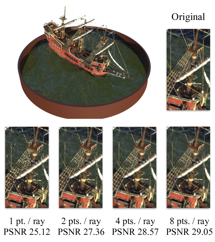
Figure 1: Novel views of a ship generated with the proposed Monte Carlo radiance estimates. For each ray we estimate density and then compute radiance at a few ray points generated using the ray density. As the above images indicate, render quality gradually improves with the number of ray samples without visible artifacts at eight points per ray.

In particular, NeRF generates an image pixel by casting a ray from a camera through the pixel and aggregating the radiance at each ray point with weights induced by the density field. Each term involves a costly neural network query, and model has a trade-off between rendering quality and computational load. In this work, we revisit the formula for the aggregated radiance computation and propose a novel approximation based on Monte Carlo methods. We compute our approximation in two stages. In the first stage, we march through the ray to estimate density. In the second stage, we construct a Monte Carlo color approximation using the density to pick points along the ray. The resulting estimate is fully-differentiable and can act as a drop-in replacement for the standard rendering algorithm used in NeRF. Fig. 1 illustrates the estimates for a varying number of samples. Compared to the standard rendering algorithm, the second stage of our algorithm avoids redundant radiance queries and can potentially reduce computation during training and inference.

Furthermore, we show that the sampling algorithm used in our Monte Carlo estimate is applicable to the hierarchical sampling scheme in NeRF. Similar to our work, the hierarchical scheme uses inverse transform sampling to pick points along a ray. The corresponding distribution is tuned using an auxiliary training task. In contrast, we derive our algorithm from a different perspective and obtain the inverse transform sampling for a slightly different distribution. With our algorithm, we were able to train NeRF end-to-end without the auxiliary task and improve the reconstruction quality. We achieve this by back-propagating the gradients through the sampler and show that the original sampling algorithm fails to achieve similar quality in the same setup.

Below, Section 2 gives a recap of neural radiance fields. Then we proceed to the main contribution of our work in Section 3, namely the rendering algorithm fueled by Monte Carlo estimates with a novel sampling procedure. In Section 4 we discuss related work. In Subsection 5.1, we compare our sampling algorithm against the hierarchical sampling scheme proposed for training NeRF. In Subsection 5.2 we evaluate our Monte Carlo approximation in a one-dimensional setting. Finally, in Subsection 5.3 we apply the proposed Monte Carlo estimate to replace the standard rendering algorithm. With an efficient neural radiance field architecture, our algorithm decreases time per training iteration at the cost of reduced reconstruction quality. We also show that our Monte Carlo estimate can be used during inference of a pre-trained model with no additional fine-tuning needed, and it can achieve better reconstruction quality at the same speed in comparison to the standard algorithm.

Our source code is available at https://github.com/GreatDrake/reparameterized-volume-sampling.

2 Neural Radiance Fields

Neural radiance fields represent 3D scenes with a non-negative scalar density field $\sigma:\mathbb{R}^{3}\rightarrow\mathbb{R}^{+}$ and a vector radiance field $c:\mathbb{R}^{3}\times\mathbb{R}^{3}\rightarrow\mathbb{R}^{3}$. Scalar field $\sigma$ represents volume density at each spatial location $\bm{x}$, and $c(\bm{x},\bm{d})$ returns the light emitted from spatial location $\bm{x}$ in direction $\bm{d}$ represented as a normalized three dimensional vector.

For novel view synthesis, NeRF [24] adapts a volume rendering algorithm that computes pixel color $C(\bm{r})$ as the expected radiance for a ray $\bm{r}=\bm{o}+t\bm{d}$ passing through a pixel from origin $\bf{o}\in\mathbb{R}^{3}$ in a direction $\bf{d}\in\mathbb{R}^{3}$. For ease of notation, we will denote density and radiance restricted to a ray $\bm{r}$ as

$$\sigma_{\bm{r}}(t):=\sigma(\bm{o}+t\bm{d})\text{\;and\;}c_{\bm{r}}(t):=c(\bm{o}+t\bm{d},\bm{d}).$$ (1)

With that in mind, the expected radiance along ray $\bm{r}$ is given as

$$C(\bm{r})=\int_{t_{n}}^{t_{f}}p_{\bm{r}}(t)c_{\bm{r}}(t)\mathrm{d}t,$$ (2)

where

$$p_{\bm{r}}(t):=\sigma_{\bm{r}}(t)\exp{\left(-\int_{t_{n}}^{t}\sigma_{\bm{r}}(s)\mathrm{d}s\right)}.$$ (3)

Here, $t_{n}$ and $t_{f}$ are near and far ray boundaries and $p_{\bm{r}}(t)$ is an unnormalized probability density function of a random variable t on a ray $\bm{r}$. Intuitively, t is the location on a ray where the portion of light coming into the point $\bm{o}$ was emitted.

To approximate the nested integrals in Eq. 2, [22] proposed to replace fields $\sigma_{\bm{r}}$ and $c_{\bm{r}}$ with a piecewise approximation on a grid $t_{n}=t_{0}<t_{1}<\dots<t_{m}=t_{f}$ and compute the formula in Eq. 2 analytically for the approximation. In particular, a piecewise constant approximation with denisty $\sigma_{i}$ and radiance $c_{i}$ within $i$-th bin $[t_{i+1},t_{i}]$ of width $\delta_{i}=t_{i+1}-t_{i}$ yields formula

$$\hat{C}(\bm{r})=\sum_{i=1}^{m}w_{i}c_{i},$$ (4)

where the weights are given by

$$w_{i}=(1-\exp(-\sigma_{i}\delta_{i}))\exp\left(-\sum_{j=1}^{i-1}\sigma_{j}\delta_{j}\right).$$ (5)

Importantly, Eq. 4 is fully differentiable and can be used as a part of gradient-based learning pipeline. To reconstruct a scene NeRF runs a gradient based optimizer to minimize MSE between the predicted color and the ground truth color averaged across multiple rays and multiple viewpoints.

While the above approximation works in practice, it involves multiple evaluations of $c$ and $\sigma$ along a dense grid. Besides that, a ray typically intersects a solid surface at some point $t\in[t_{n},t_{f}]$. In this case, probability density $p_{\bm{r}}(t)$ will concentrate its mass near $t$ and, as a result, most of the terms in Eq. 4 will make negligible contribution to the sum. To approach this problem, NeRF employs a hierarchical sampling scheme. Two networks are trained simultaneously: coarse (or proposal) and fine. Firstly, the coarse network is evaluated on a uniform grid of $N_{c}$ points and a set of weights $w_{i}$ is calculated as in Eq. 5. Normalizing these weights produces a piecewise-constant PDF along the ray. Then $N_{f}$ samples are drawn from this distrubution and the union of the first and the second sets of points is used to evaluate the fine network and compute the final color estimation. The coarse network is also trained to predict ground truth colors, but the color estimate for the coarse network is calculated only using the first set of $N_{c}$ points.

3 Reparameterized Volume Sampling and Radiance Estimates

3.1 Reparameterized Expected Radiance Estimates

Monte Carlo method gives a natural way to approximate the expected color. For example, given $k$ i.i.d. samples $t_{1},\dots,t_{k}\sim p_{\bm{r}}(t)$ and the normalization constant $y_{f}:=\int_{t_{n}}^{t_{f}}p_{\bm{r}}(t)\mathrm{d}t$, the sum

$$\hat{C}_{MC}(\bm{r})=\frac{y_{f}}{k}\sum_{i=1}^{k}c_{\bm{r}}(t_{i})$$ (6)

is an unbiased estimate of the expected radiance in Eq. 2. Moreover, samples $t_{1},\dots,t_{k}$ belong to high-density regions of $p_{\bm{r}}$ by design, thus for a degenerate density $p_{\bm{r}}$ even a few samples would provide an estimate with low variance. Importantly, unlike the approximation in Eq. 4, the Monte Carlo estimate depends on scene density $\sigma$ implicitly through sampling algorithm and requires a custom gradient estimate for the parameters of $\sigma$. We propose a principled end-to-end differentiable algorithm to generate samples from $p_{\bm{r}}(t)$.

Out solution is primarily inspired by the reparameterization trick [14, 32]. We change the variable in Eq. 2. For ${F_{\bm{r}}(t):=1-\exp{\left(-\int_{t_{n}}^{t}\sigma_{\bm{r}}(s)\mathrm{d}s\right)}}$ and $y:=F_{\bm{r}}(t)$ we rewrite

$$C(\bm{r}) =\int_{t_{n}}^{t_{f}}c_{\bm{r}}(t)p_{\bm{r}}(t)\mathrm{d}t$$ (7)

$$=\int_{y_{n}}^{y_{f}}c_{\bm{r}}(F_{\bm{r}}^{-1}(y))\mathrm{d}y$$ (8)

$$=\int_{0}^{1}y_{f}c_{\bm{r}}(F_{\bm{r}}^{-1}(y_{f}u))\mathrm{d}u.$$ (9)

The integral boundaries are $y_{n}:=F_{\bm{r}}(t_{n})=0$ and $y_{f}:=F_{\bm{r}}(t_{f})$. Function $F_{\bm{r}}(t)$ acts as the cumulative distribution function of the variable t with a single exception that, in general, $F_{\bm{r}}(t_{f})\neq 1$. In volume rendering, $F_{\bm{r}}(t)$ is called opacity function with $y_{f}$ being equal to overall pixel opaqueness. After the first change of variables in Eq. 8, the integral boundaries depend on opacity $F_{\bm{r}}$ and, as consequence, on ray density $\sigma_{\bm{r}}$. We further simplify the integral by changing the integration boundaries to $[0,1]$ and substituting $y_{n}=0$.

Given the above derivation, we construct the reparameterized Monte Carlo estimate for the right-hand side integral in Eq. 9

$$\hat{C}_{MC}^{R}(\bm{r}):=\frac{y_{f}}{k}\sum_{i=1}^{k}c_{\bm{r}}(F_{\bm{r}}^{-1}(y_{f}u_{i})),$$ (10)

with $k$ i.i.d. $U[0,1]$ samples $u_{1},\dots,u_{k}$. It is easy to show that estimate in Eq. 10 is an unbiased estimate of expected color in Eq. 2 and its gradient is an unbiased estimate of the gradient of the expected color $C(\bm{r})$. Additionally, we propose to replace the uniform samples $u_{1},\dots,u_{k}$ with uniform independent samples within regular grid bins $v_{i}\sim U[\tfrac{i-1}{k+1},\tfrac{i}{k+1}],i=1,\dots,k$. The latter samples yield a stratified variant of the estimate in Eq. 10 and, most of the time, leads to lower variance estimates (see Appendix 5.2).

In the above estimate, random samples $u_{1},\dots,u_{k}$ do not depend on volume density $\sigma_{\bm{r}}$ or color $c_{\bm{r}}$. Essentially, for the reparameterized Monte Carlo estimate we generate samples from $p_{\bm{r}}(t)$ using inverse cumulative distribution function $F_{\bm{r}}^{-1}(y_{f}u)$. In what follows, we coin the term reparameterized volume sampling (RVS) for the sampling procedure. However, in practice we cannot compute $F_{\bm{r}}$ analytically and can only query $\sigma_{\bm{r}}$ at certain ray points. Thus, in the following section, we introduce approximations of $F_{\bm{r}}$ and its inverse.

3.2 Opacity Approximations

Expected radiance estimate in Eq. 10 relies on opacity $F_{\bm{r}}(t)=1-\exp\left(-\int_{t_{n}}^{t}\sigma_{\bm{r}}(s)\mathrm{d}s\right)$ and its inverse $F^{-1}_{\bm{r}}(y)$. We propose to approximate the opacity using a piecewise density field approximation. Fig. 2 illustrates the approximations and ray samples obtained through opacity inversion.

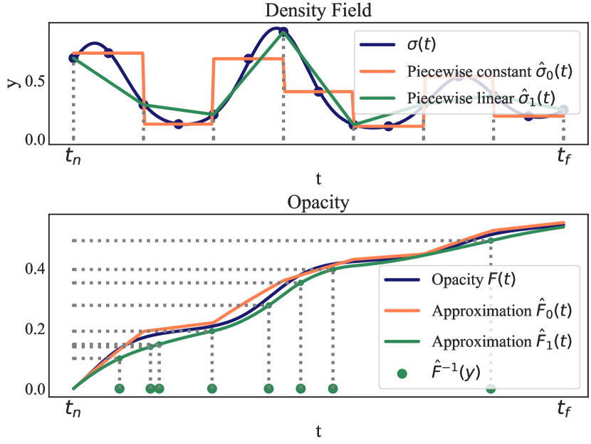
Figure 2: Illustration of opacity inversion. On the left, we approximate density field $\sigma_{\bm{r}}$ with a piecewise constant and a piecewise linear approximation. On the right, we approximate opacity $F_{\bm{r}}(t)$ and compute $F^{-1}_{\bm{r}}(y_{f}u)$ for $u\sim U[0,1]$.

To construct the approximation, we take a grid $t_{n}=t_{0}<t_{1}<\dots<t_{m}=t_{f}$ and construct either a piecewise constant or a piecewise linear approximations. In the former case, we pick a point within each bin $t_{i}\leq\hat{t}_{i}\leq t_{i+1}$ and approximate density with $\sigma_{\bm{r}}(\hat{t}_{i})$ inside the corresponding bin. In the latter case, we compute $\sigma_{\bm{r}}$ in the grid points and interpolate the values between the grid points. Importantly, for a non-negative field these two approximations are also non-negative. Then we compute $\int_{t_{n}}^{t}\sigma_{\bm{r}}(s)\mathrm{d}s$ , which is as a sum of rectangular areas in the piecewise constant case

$$I_{0}(t)=\sum_{j=1}^{i}\sigma_{\bm{r}}(\hat{t}_{j})(t_{j}-t_{j-1})+\sigma_{\bm{r}}(\hat{t}_{i})(t-t_{i}).$$ (11)

Analogously, the integral approximation $I_{1}(t)$ in the piecewise linear case is a sum of trapezoidal areas.

Given these approximations, we can approximate $y_{f}$ and $F_{\bm{r}}$ in Eq. 10. We generate samples on a ray based on inverse opacity $F^{-1}_{\bm{r}}(y)$ by solving the equation

$$y_{f}u=F_{\bm{r}}(t)=1-\exp\left(-\int_{t_{n}}^{t}\sigma_{\bm{r}}(s)\mathrm{d}s\right)$$ (12)

for $t$, where $u\in[0,1]$ is a random sample. We rewrite the equation as $-\log(1-y_{f}u)=\int_{t_{n}}^{t}\sigma_{\bm{r}}(s)\mathrm{d}s$ and note that integral approximations $I_{0}(t)$ and $I_{1}(t)$ are monotonic piecewise linear and piecewise quadratic functions. We obtain the inverse by first finding the bin that contains the solution and then solving a linear or a quadratic equation. Crucially, the solution $t$ can be seen as a differentiable function of density field $\sigma_{\bm{r}}$ and we can back-propagate the gradients w.r.t. $\sigma_{\bm{r}}$ through $t$. We provide explicit formulae for $t$ for both approximations in Appendix A.1 and discuss the solutions crucial for the numerical stability in Appendix A.2. In Appendix A.3, we implement the algorithm and draw parallels with earlier work. Additionally, in Appendix A.4 we discuss an alternative approach to calculating inverse opacity and its gradients. We use piecewise linear approximation in Subsection 5.1 and piecewise constant in Subsection 5.3.

3.3 Application to Hierarchical Sampling

Finally, we propose to apply our RVS algorithm to the hierarchical sampling scheme originally proposed in NeRF. Here we do not change the final color approximation, utilizing the original one (Eq.4), but modify the way the coarse density network is trained. The method we introduce consists of two changes to the original scheme. Firstly, we replace sampling from piecewise-constant PDF along the ray defined by weights $w_{i}$ (see Section 2) with our RVS sampling algorithm that uses piecewise linear approximation of $\sigma_{\bm{r}}$ and generates samples from $p_{r}(t)$ using inverse CDF. Secondly, we remove the auxiliary reconstruction loss imposed on the coarse network. Instead, we propagate gradients through sampling. This way, we eliminate the need for auxiliary coarse network losses and train the network to solve the actual task of our interest: picking the best points for evaluation of the fine network. All components of the model are trained together end-to-end from scratch. In Subsection 5.1, we refer to the coarse network as the proposal network, since such naming better captures its purpose.

4 Related Work

Monte-Carlo estimates for integral approximations. In this work, we revisit the algorithm introduced to approximate the expected color in [22]. Currently, it is the default solution in multiple of works on neural radiance fields. [22] approximate density and radiance fields with a piecewise constant functions along a ray and compute Eq.  2 as an approximation. Instead, we reparameterize Eq. 2 and construct Monte-Carlo estimates for the integral. To compute the estimates in practice we use piecewise approximations only for the density field. The cumulative density function (CDF) used in our estimates involves integrating density field along a ray. [19] construct field anti-derivatives to accelerate inference. While they use the anti-derivatives to compute 2 on a grid with fewer knots, the anti-derivatives can be applied in our sampling method based on the inverse CDF without resorting to piecewise approximations.

In the past decade, integral reparameterizations became a common practice in generative modeling [15, 32] and approximate Bayesian inference [5, 10, 26]. Similar to Equation 2, objectives in these areas require optimizing expected values with respect to distribution parameters. We refer readers to [25] for a systematic overview. Notably, in computer graphics, [21] apply reparameterization to estimate gradients of path traced images with respect to scene parameters.

NeRF acceleration through architecture and sparsity. Since the original NeRF work [24], a number of approaches that aim to improve the efficiency of the model have been proposed. One family of methods tries to reduce the time required to evaluate the field. It includes a variety of architectures combining Fourier features [34] and grid-based features [11, 33, 36, 31]. Besides grids, some works exploit space partitions based on Voronoi diagrams [30], trees [13, 37] and even hash tables [27]. These architectures generally trade-off inference speed for parameter count. TensorRF [6] stores the grid tensors in a compressed format to achieve both high compression and fast performance. On top of that, skipping field queries for the empty parts of a scene additionally improves rendering time [17]. Recent works (such as [12, 9, 20, 18, 33, 27]) manually exclude low-weight components in Eq 4 to speed up rendering during training and inference. Below we show that our Monte Carlo algorithm is compatible with fast architectures and sparse density fields, achieving comparable speed up by using a few radiance evaluations.

Anti-aliased scene representations. Mip-NeRF [2], Mip-NeRF 360 [3] and a more recent Zip-NeRF [4] represent a line of work that modifies scene representations. Relevant to our research is the fact that these models employ modifications of the original hierarchical sampling scheme where the coarse network parameterizes some density field. Mip-NeRF parameterizes the coarse and the fine fields by the same neural network that represents the scene at a continuously-valued scale. Mip-NeRF 360 and Zip-NeRF use a separate model for proposal density, but train it to mimick the fine density rather than independently reconstructing the image. This means that our method for training the proposal density field can be potentially used to improve the performance of these models and simplify the training algorithm.

Algorithms for picking ray points. [24] employs a hierarchical scheme to generate ray points using an auxiliary density and color fields. Since then, a number of other methods for picking ray points, which focus on real-time rendering and aim to improve the efficiency of NeRF, have been proposed. DoNeRF [28] uses a designated depth oracle network supervised with ground truth depth maps. TermiNeRF [29] foregoes the depth supervision by distilling the sampling network from a pre-trained NeRF model. NeRF-ID [1] adds a separate differentiable proposer neural network to the original NeRF model that maps outputs of the coarse network into a new set of samples. The model is trained in two stage procedure together with NeRF. Authors of NeuSample [7] use a sample field that directly transforms rays into point coordinates. Sample field can be further fine-tuned for rendering with smaller number of samples. AdaNeRF [16] proposes to use a sampling and a shading network. Samples from sampling network are processed by shading network that tries to predict the importance of samples and cull the samples with low importance. One of the key merits of our approach in comparison to these works is simplicity. We simplify the original NeRF training procedure, while other works only build upon it, adding new components, training stages, constraints, or losses. Moreover, the absence of reliance on additional neural network components (not responsible for density or radiance) for sampling makes our approach better suited for fast NeRF architectures. Finally, our approach is suitable for end-to-end training of NeRF models from scratch, whereas the works mentioned above use pre-trained NeRF models or multiple training stages.

5 Experiments

5.1 End-to-end Differentiable Hierarchical Sampling

In this section, we evaluate the proposed approach to hierarchical volume sampling.

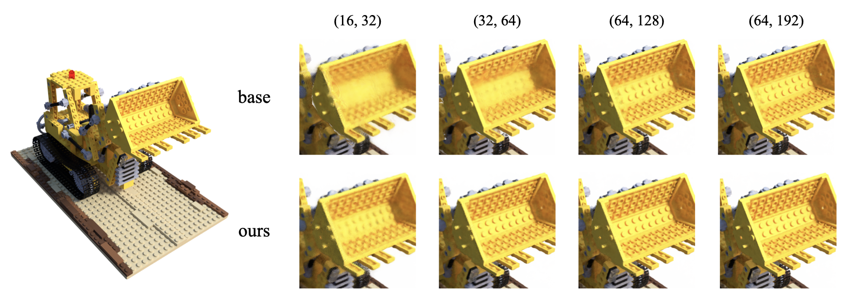
Figure 3: Comparison between renderings of test-set view on the Lego scene (Blender). Rows correspond to different $(N_{p},N_{f})$ configurations. NeRF baseline has difficulties in reconstructing fine details for $(16,32)$ and $(32,64)$ configurations, and some parts remain blurry even in $(64,128)$ and $(64,192)$ configurations, while our method already produces realistic reconstruction for $(32,64)$ configuration.

Experimental setup. We do the comparison by fixing some training setup and training two models from scratch: one NeRF model is trained using the procedure proposed in [24] (further denoted as NeRF in the results), and the other one is trained using our modification described in Subsection 3.3 (further denoted as RVS). For both models, the final color approximation is computed as in Eq. 4, so the difference only appears in the proposal component.

We trained all models for 500k iterations using the same hyperparameters as in the original paper with minor differences. We replaced ReLU density output activation with Softplus. The other difference is that we used smaller learning rate for the proposal density network in our method (start with $5\times 10^{-5}$ and decay to $5\times 10^{-6}$) but the same for the fine network (start with $5\times 10^{-4}$ and decay to $5\times 10^{-5}$). We observed that decreasing the proposal network learning rate improves stability of our method. We ran the default NeRF training algorithm in our experiments with the same learning rates for proposal and fine networks. Further in the ablation study we show that decreasing proposal network learning rate only decreases the performance of the base algorithm. We used PyTorch implementation [35] of NeRF in our experiments.

Table 1: Comparison on the Lego scene of Blender dataset between NeRF training algorithm and our modification depending on the number of proposal and fine network evaluations per ray $(N_{p},N_{f})$. The $(64,192)$ configuration is the one originally used in NeRF. Training time column depicts relative training time on a single NVIDIA A100 GPU (1.0 being 12 hours).

	Evaluations		Train	PSNR $\uparrow$	SSIM $\uparrow$	LPIPS $\downarrow$
	$N_{p}$	$N_{f}$	time
NeRF	16	32	0.39	27.09	0.913	0.121
RVS	16	32	0.37	29.18	0.928	0.112
NeRF	32	64	0.52	30.11	0.947	0.070
RVS	32	64	0.48	31.89	0.955	0.066
NeRF	64	128	0.79	32.14	0.958	0.053
RVS	64	128	0.76	32.80	0.963	0.051
NeRF	64	192	1.0	32.69	0.962	0.048
RVS	64	192	0.98	33.03	0.964	0.047

Table 2: Comparison with NeRF on Blender and LLFF datasets in $(N_{p}=32,N_{f}=64)$ configuration.

	Blender Dataset
	PSNR $\uparrow$	SSIM $\uparrow$	LPIPS $\downarrow$
NeRF	29.49	0.934	0.085
RVS	30.26	0.939	0.082
	LLFF Dataset
	PSNR $\uparrow$	SSIM $\uparrow$	LPIPS $\downarrow$
NeRF	26.01	0.796	0.273
RVS	26.24	0.799	0.270

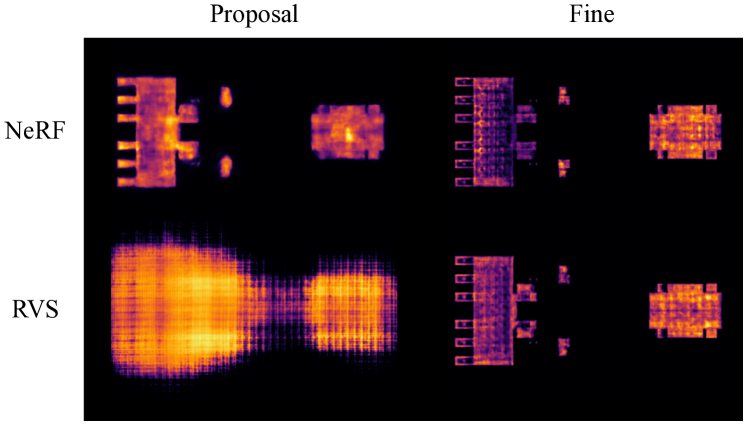
Figure 4: Visualizations across 2D slice of proposal and fine densities learnt on the Lego scene in $(32,64)$ configuration. Brighter pixels correspond to larger density values.

Comparative evaluation. We start the comparison on the Lego scene of the synthetic Blender dataset [24] for different $(N_{p},N_{f})$ configurations that correspond to number of proposal and fine network evaluations. Note that this $N_{p}$, $N_{f}$ notation does not directly correspond to the $N_{c}$, $N_{f}$ notation used in Section 2 since the original NeRF model evaluates the fine network in $N_{c}$ + $N_{f}$ points. For more details on training configurations and options for picking points for fine network evaluation, see Appendix C. The results are presented in Table 1. Our method outperformed the baseline across all configurations and all metrics, with the only exception of LPIPS in $(64,192)$ configuration, where it showed similar performance. We observe that the improvement is more significant for smaller $(N_{p},N_{f})$. Our method also has a minor speedup over the baseline due to the fact that the former does not use the radiance component of the proposal network. Fig. 3 in visualizes test-set view renderings of models trained by two methods.

We also visualize proposal and fine densities learned by two algorithms in Fig. 4. Figures are constructed by fixing some value of $z$ coordinate and calculating the density on $(x,y)$-plane. While fine density visualizations look very similar, proposal densities turn out very different. This happens due to the fact that the original algorithm trains the proposal network to reconstruct the scene (but using smaller number of points for color estimation), while our algorithm trains this network to sample points for fine network evaluation that would lead to a better overall reconstruction. We believe that this may also explain the improved rendering quality that our method shows.

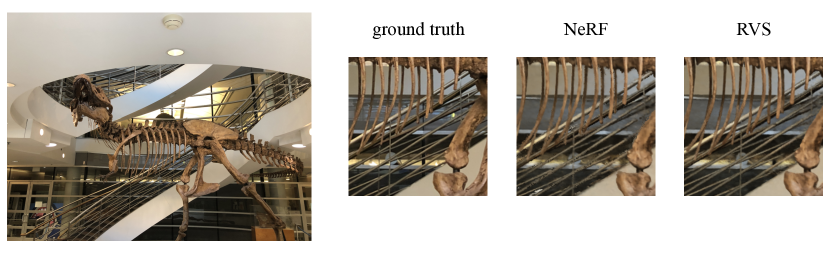
Figure 9: Comparison between renderings of test-set view on T-Rex scene (LLFF) for $(32,64)$ configuration. Artifacts can be seen on railings and bones in the NeRF render, while such artifacts are absent in the reconstruction produced by our model.

Next, we evaluated our method on all scenes from Blender, as well as the LLFF [23] dataset containing real scenes. Table 2 depicts the results averaged across all scenes. The results for individual scenes can be found in Table 10 and Table 11 in Appendix E. Our approach showed improvement over the baseline on all scenes of Blender dataset. While the improvement is less pronounced on LLFF dataset, it is still present across all metrics on average. Fig. 9 in Appendix D visually depicts the quality of reconstruction on T-Rex scene.

Unbounded scenes. In addition, we evaluated our approach with NeRF++ [38] modification designed for unbounded scenes. NeRF++ utilizes the same hierarchical scheme as the original NeRF, so we ran the same setup as previously: one model is trained using the original procedure, and for the other one we replace the sampling algorithm with RVS and propagate gradients through sampling instead of using a separate reconstruction loss for the proposal network. We did not modify any hyperparameters in comparison to [38] apart from using a using a smaller $(N_{p},N_{f})$ configuration and a smaller proposal learning rate in our approach, the same as in the previous experiments. We ran the comparison on LF and T&T datasets [38] containing unbounded real scenes. The results are presented in Table 3. Our approach also showed improvement over NeRF++ across all metrics on both datasets. Table 12 and Table 13 in Appendix E present the results for individual scenes.

Table 3: Comparison with NeRF++ on LF and T&T datasets in $(N_{p}=32,N_{f}=64)$ configuration.

	LF Dataset
	PSNR $\uparrow$	SSIM $\uparrow$	LPIPS $\downarrow$
NeRF++	23.99	0.784	0.287
RVS	24.63	0.812	0.253
	T&T Dataset
	PSNR $\uparrow$	SSIM $\uparrow$	LPIPS $\downarrow$
NeRF++	19.21	0.612	0.493
RVS	19.62	0.622	0.472

Table 4: Ablation study with NeRF on Blender dataset in $(N_{p}=32,N_{f}=64)$ configuration.

	Blender Dataset
	PSNR $\uparrow$	SSIM $\uparrow$	LPIPS $\downarrow$
NeRF (decreased prop. lr)	29.23	0.932	0.090
NeRF (union of points)	29.06	0.929	0.096
NeRF	29.49	0.934	0.085
RVS (NeRF sampling)	29.07	0.929	0.095
RVS	30.26	0.939	0.082

Ablation study. Finally, we ablated the influence of some components of our approach on the results. Table 4 presents the ablation study results. Firstly, we ran the baseline with decreased learning rate for the proposal network, thus fully matching all training hyperparameters with our method. This only reduced all metrics in comparison to the baseline. Then, we ran our approach, but replaced our algorithm that draws samples from the proposal distribution with the sampling algorithm originally proposed in NeRF. Even though the original work does not propagate gradients through sampling, the algorithm is still end-to-end differentiable, thus the setup is plausible. It also produced results that fell behind the baseline. This shows that while both algorithms are differentiable, ours is better suited for end-to-end optimization. We discuss the differences between two algorithms in Appendix A.3. Finally, we ran the baseline with different strategy for picking fine points (see Appendix C for detailed discussion), which also led to degradation of the baseline performance.

5.2 Radiance Estimates for a Single Ray

In this section, we evaluate the proposed Monte Carlo radiance estimate (see Eq. 10) in a one-dimensional setting. In this experiment, we assume that we know density in advance and show how the estimate variance depends on number of radiance calls. Compared to sampling approaches, the standard approximation from Eq. 4 has zero variance but does not allow controlling number of radiance calls.

Our experiment models light propagation on a single ray in two typical situations. The upper row of Fig. 5 defines a scalar radiance field (orange) $c_{\bm{r}}(t)$ and opacity functions (blue) $F_{\bm{r}}(t)$ for "Foggy" and "Wall" density fields. The first models a semi-transparent volume, which often occurs after model initialization during training. In the second light is emitted from a single point on a ray, which is common in applications.

For the two fields we estimated the expected radiance $C(\bm{r})=\int_{t_{n}}^{t_{f}}c_{\bm{r}}(t)\mathrm{d}F_{\bm{r}}(t)$. We considered two baseline methods (both in red in Fig. 5): the first was a Monte Carlo estimate of $C$ obtained with uniform distribution on a ray $U[t_{n},t_{f}]$, and its stratified modification with a uniform grid $t_{n}=t_{0}<\dots<t_{k}=t_{f}$ (note that here we use $k$ to denote the number of samples, not the number of grid points $m$ in piecewise density approximation):

$$\hat{C}_{\text{IW}}(\bm{r})=\sum_{i=1}^{k}(t_{i}-t_{i-1})c_{\bm{r}}(\tau_{i})\frac{\mathrm{d}F_{\bm{r}}}{\mathrm{d}t}\bigg{\rvert}_{t=\tau_{i}},$$ (13)

where $\tau_{i}\sim U[t_{i-1},t_{i}]$ are independent uniform bin samples. We compared the baseline against estimate from Eq. 10 and its stratified modification. All estimates are unbiased. Therefore, we only compared the estimates variances for a varying number of samples $m$. In all setups, our stratified estimate uniformly outperformed the baselines. For the more challenging "foggy" field, approximately $k=32$ samples were required to match the baseline performance for $k=128$. We matched the baseline with only a $k=4$ samples for the "wall" field. Inverse transform sampling requires only a few points for degenerate distributions.

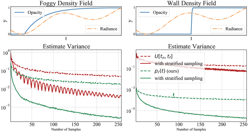
Figure 5: Color estimate variance compared for a varying number of samples. The upper plot illustrates underlying opacity function on a ray; the lower graph depicts variance in logarithmic scale. Compared to a naive estimate of the integral with uniform samples (dashed red), inverse transform sampling exhibits lower variance (dashed green). Stratified sampling improves variance in both setups (solid lines).

5.3 Scene Reconstruction with Monte Carlo Estimates

In this section, we evaluate the proposed Monte Carlo radiance estimate as a part of rendering algorithm for scene reconstruction. Given an accurate density field approximation, our color estimate is unbiased for any given number of samples $k$. Therefore, our estimate is especially suitable for architectures that can evaluate the density field faster than the radiance field. As an example, we picked a recent voxel-based radiance field model DVGO [33] that parametrizes density field as a voxel grid and relies on a combination of voxel grid and a view-dependent neural network to parameterize radiance. In our experiments, we took the default model parameters and only replaced the rendering algorithm.

Table 5: Training iteration times and peak memory consumption for different color approximations.

DVGO Renderer	Speed	Memory
Default w/o sparisty	24 it/s	9 GB
Default w/ sparsity	160 it/s	5 GB
MC + RVS, $k=128$	20 it/s	8 GB
MC + RVS, $k=8$	170 it/s	5 GB
MC + RVS, $k=1$	260 it/s	5 GB

Experimental setup & comparative evaluation. In Table 5, we report iterations per second and peak memory consumption on the Lego scene of Blender dataset during training. One of the primary goals of DVGO was to reduce the training time of a scene model. To achieve that goal, the authors mask components in the sum in Eq. 4 that have weights below a certain threshold $\alpha$. We achieve a similar effect without thresholding: $k=8$ samples yield a comparable $\times 6$ speed up and with fewer samples, we reduce iteration time even further. However, the speed-up in our estimate comes at cost of additional estimate variance. Next, we evaluated the effect of additional variance on the rendering fidelity. In Fig. 6, we report test PSNR on a fixed pre-trained Lego scene representation for both rendering algorithms. Our algorithm achieves the same average PSNR with $k=8$ samples and outperforms the default rendering algorithm in case of a higher sparsity threshold $\alpha$.

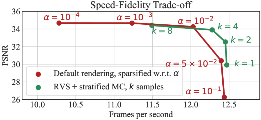
Figure 6: Test-time rendering quality as a function of rendering speed. Given a scene representation pre-trained with the standard rendering algorithm, we evaluate rendering algorithms at various configurations.

In Table 6, we report the performance of models trained with various color estimates (see Appendix E for per-scene results). We trained a model with $k=4$ samples using $\times\tfrac{3}{2}$ more training steps than with $k=8$ samples aiming to achieve similar training times. Additionally, we considered a model that chooses the number of samples $k$ on each ray adaptively between $4$ and $48$ based on the number of grid points with high density. The adaptive number of samples allowed to reduce estimate variance without a drastic increase in training time. We evaluate our models with $k=64$ samples to mitigate the effect of variance on evaluation. As Table 6 indicates, the training algorithm with our color approximation fails to outperform the base algorithm in terms of reconstruction quality, however it allows for the faster training of the model.

Table 6: Scene reconstruction results for Blender dataset.

DVGO Renderer	Train time (min)	PSNR$\uparrow$	SSIM$\uparrow$	LPIPS$\downarrow$
Default w/ sparsity	2:48	31.90	0.956	0.054
MC + RVS, $k=4$	2:24	31.19	0.951	0.059
MC + RVS, $k=8$	2:00	31.13	0.951	0.059
MC + RVS, adaptive $k$	2:54	31.44	0.953	0.056

Table 7: Ablation study of the Lego scene.

Ablated Feature	PSNR
MC + RVS with adaptive $k$	$33.85$
Training steps $(\times 7)$	$+0.28$
Training steps $(\times 7)$	$+0.28$
Monte Carlo samples $(\times 2\text{\ on avg.})$	$+0.15$
Dense grid on rays $(\times 2)$	$+0.29$
Unbiased loss $L_{2}(\mathbb{E}\hat{C},C_{gt})$	$+0.25$
Density grid resolution $(160^{3}\rightarrow 256^{3})$	$+0.63$
Radiance grid resolution $(160^{3}\rightarrow 256^{3})$	$+0.08$
$\sigma$ + $c$ resolution $(160^{3}\rightarrow 256^{3})$	$+0.86$
DVGO	$34.64$

Ablation study. We ablated the proposed algorithm on the Lego scene to gain further insights into the difference in reconstruction fidelity. Specifically, we ablated parameters affecting optimization aiming to match the reconstruction quality of the default algorithm. The results are given in Table 7. The increase in training steps or the number of samples improved the performance but did not lead to matching results. Increased spline density improved both our model and the baseline to the same extent. We also noticed that the standard objective estimated the expected loss $\mathbb{E}L_{2}(\hat{C},C_{gt})$ rather than the loss at expected radiance $L_{2}(\mathbb{E}\hat{C},C_{gt})$ which leads to an additional bias towards low-variance densities. The estimate $(\hat{C}_{1}-C_{gt})(\hat{C}_{2}-C_{gt})$ with two i.i.d. color estimates is an unbiased estimate of the latter and allows reconstructing non-degenerate density fields, but the estimate has little effect in case of degenerate densities omnipresent in 3D scenes. Finally, with denser ray grid our algorithm surpassed the baseline PSNR of 34.67 at twice the training time. For qualitative comparison, in Appendix D, we visualize the differences in reconstructed models and in renders reported in Fig. 6.

To summarise, training with reparameterized volume sampling currently does not fully match the fidelity of the standard approach. At the same time, Monte Carlo radiance estimates provide a straightforward mechanism to control both training and inference speed.

6 Conclusion

The core of our contribution is an end-to-end differentiable ray point sampling algorithm. We utilize it to construct an alternative rendering algorithm based on Monte Carlo, which provides an explicit mechanism to control rendering time during the inference and training stages. While it is able to outperform the standard rendering algorithm at the inference stage given a pre-trained model, it achieves lower reconstruction quality when used during training, which suggests areas for future research. At the same time, we show that the proposed sampling algorithm improves scene reconstruction in hierarchical models and simplifies the training approach by disposing of auxiliary losses.

Appendix A Inverse Opacity Calculation

A.1 Inverse Functions for Density Integrals

In this section, we derive explicit formulae for the density integral inverse used in inverse opacity.

A.1.1 Piecewise Constant Approximation Inverse

We start with a formula for the integral

$$I_{0}(t)=\sum_{j=1}^{i}\sigma_{\bm{r}}(\hat{t}_{j})(t_{j}-t_{j-1})+\sigma_{\bm{r}}(\hat{t}_{i})(t-t_{i})$$ (14)

and solve for $t$ equation

$$y=I_{0}(t).$$ (15)

The equation above is a linear equation with solution

$$t=t_{i}+\frac{y-\sum_{j=1}^{i}\sigma_{\bm{r}}(\hat{t}_{j})(t_{j}-t_{j-1})}{\sigma_{\bm{r}}(\hat{t}_{i})}.$$ (16)

In our implementation we add small $\epsilon$ to the denominator to improve stability when $\sigma_{\bm{r}}(\hat{t}_{i})\approx 0$.

A.1.2 Piecewise Linear Approximation Inverse

The piecewise linear density approximation yield a piecewise quadratic function

$$I_{1}(t)=\sum_{j=1}^{i}\frac{\sigma_{\bm{r}}(t_{j})+\sigma_{\bm{r}}(t_{j-1})}{2}(t_{j}-t_{j-1})+\frac{(\sigma_{\bm{r}}(t_{i})+\bar{\sigma}_{\bm{r}}(t))}{2}(t-t_{i}),$$ (17)

where $\bar{\sigma}_{\bm{r}}(t)=\sigma_{\bm{r}}(t_{i})\frac{t_{i+1}-t}{t_{i+1}-t_{i}}+\sigma_{\bm{r}}(t_{i+1})\frac{t-t_{i}}{t_{i+1}-t_{i}}$ is the interpolated density at $t$. Again, we solve

$$y=I_{1}(t)$$ (18)

for $t$. We change the variable to $\Delta t:=t-t_{i}$ and note that terms $a$ and $c$ in quadratic equation

$$0=a\Delta t^{2}+b\Delta t+c$$ (19)

will be

$$a =\frac{\sigma_{\bm{r}}(t_{i+1})-\sigma_{\bm{r}}(t_{i})}{2}$$ (20)

$$c =\left(\sum_{j=1}^{i}\frac{\sigma_{\bm{r}}(t_{j})+\sigma_{\bm{r}}(t_{j-1})}{2}(t_{j}-t_{j-1})-y\right)\times(t_{i+1}-t_{i})$$ (21)

and with a few algebraic manipulations we find the linear term

$$b=\sigma_{\bm{r}}(t_{i})\times(t_{i+1}-t_{i}).$$ (22)

Since our integral monotonically increases, we can deduce that the root $\Delta t$ must be

$$\Delta t=\tfrac{-b+\sqrt{b^{2}-4ac}}{2a}.$$ (23)

However, this root is computationally unstable when $a\approx 0$. The standard trick is to rewrite the root as

$$\Delta t=\tfrac{2c}{b+\sqrt{b^{2}-4ac}}.$$ (24)

For computational stability, we add small $\epsilon$ to the square root argument. See the supplementary notebook for details.

A.2 Numerical Stability in Inverse Opacity

Inverse opacity input $y$ is a combination of a uniform sample $u$ and ray opacity $y_{f}=1-\exp\left(-\int_{t_{n}}^{t_{f}}\sigma_{\bm{r}}(s)\mathrm{d}s\right)$:

$$y=-\log(1-y_{f}u).$$ (25)

The expression above is a combination of a logarithm and exponent. We rewrite it to replace with more reliable $\operatorname{logsumexp}$ operator:

$$y=-\log\left(\exp(\log(1-u))+\exp(\log u-\int_{t_{n}}^{t_{f}}\sigma_{\bm{r}}(s)\mathrm{d}s)\right).$$ (26)

In practice, for opaque rays $\int_{t_{n}}^{t_{f}}\sigma_{\bm{r}}(s)\mathrm{d}s\approx 0$ implementation of $\operatorname{logsumexp}$ becomes computationally unstable. In this case, we replace $y$ with a first order approximation $u\cdot\int_{t_{n}}^{t_{f}}\sigma_{\bm{r}}(s)\mathrm{d}s$.

A.3 Parallels with Prior Work and Algorithm Implementation

Original NeRF architecture uses inverse transform sampling to generate a grid for a fine network. They define a distribution based on Eq 2 with piecewise constant density. In turn, we define inverse transform sampling for a distribution induced by a piecewise interpolation of $\sigma_{\bm{r}}$ in Eq. 2. The two approximation approaches yield distinct sampling algorithms. In the listing below, we provide a numpy implementation of the two algorithms to highlight the difference. The implementation assumes a single ray for bravity. We rewrite NeRF sampling algorithm in an equivalent simplified form to facilitate the comparison. For simplicity, we provide implementation of RVS only for a piecewise constant approximation of $\sigma$. The inversion algorithm described in Appendix A.1 is hidden under the hood of np.interp().

The interpolation scheme in our algorithm can be seen as linear interpolation of density field rather than probabilities. As a result, samples follow the Beer-Lambert law within each bin. The law describes light absorption in a homogeneous medium. In contrast, the hierarchical sampling scheme in NeRF interpolates exponentiated densities. We speculate that the numerical instability of exponential function makes the latter algorithm less suitable for end-to-end optimization (as observed in Table 4).

import numpy as np

def inverse_cdf(u, sigmas, ts, sampling_mode):
    """ Get inverse CDF sample

    Arguments:
    u - array of uniform random variables
    sigmas - array of density values on a grid
    ts - array of grid knots
    """
    # Compute $\int_{t_0}^{t_i} \sigma(s) ds$
    bin_integrals = sigmas * np.diff(ts)
    prefix_integrals = np.cumsum(bin_integrals)
    prefix_integrals = np.concatenate([np.zeros(1), prefix_integrals])
    # Get inverse CDF argument
    rhs = -np.expm1(-bin_integrals.sum()) * u
    if sampling_mode == ’rvs’:  # interpolate $\int \sigma(s) ds$
        return np.interp(-np.log1p(-rhs), prefix_integrals, ts)
    elif sampling_mode == ’nerf’:  # interpolate CDF
        return np.interp(rhs, -np.expm1(-prefix_integrals), ts)

A.4 Implicit Inverse Opacity Gradients

To compute the estimates in Eq. 10, we need to compute the inverse opacity $F_{\bm{r}}^{-1}(y)$ along with its gradient. In the main paper, we invert opacity explicitly with a differentiable algorithm. Alternatively, we could invert $F_{\bm{r}}(t)=1-\exp{\left(-\int_{t_{n}}^{t}\sigma_{\bm{r}}(s)\mathrm{d}s\right)}$ with binary search. This approach can be used in situations when the formula for inverse opacity cannot be explicitly derived.

Opacity $F_{\bm{r}}(t)$ is a monotonic function and for $y\in(y_{n},y_{f})=(F_{\bm{r}}(t_{n}),F_{\bm{r}}(t_{f}))$ the inverse lies in $(t_{n},t_{f})$. To compute $F_{\bm{r}}^{-1}(y)$, we start with boundaries $t_{l}=t_{n}$ and $t_{r}=t_{f}$ and gradually decrease the gap between the boundaries based on the comparison of $F_{\bm{r}}(\tfrac{t_{l}+t_{r}}{2})$ with $y$. Importantly, such procedure is easy to parallelize across multiple inputs and multiple rays.

However, we cannot back-propagate through the binary search iterations and need a workaround to compute the gradient $\tfrac{\partial t}{\partial\theta}$ of $t(\theta)=F_{\bm{r}}^{-1}(y,\theta)$. To do this, we follow [8] and compute differentials of the right and the left hand side of equation $y(\theta)=F_{\bm{r}}(t,\theta)$

$$\frac{\partial y}{\partial\theta}\mathrm{d}\theta=\frac{\partial F_{\bm{r}}}{\partial t}\frac{\partial t}{\partial\theta}\mathrm{d}\theta+\frac{\partial F_{\bm{r}}}{\partial\theta}\mathrm{d}\theta.$$ (27)

By the definition of $F_{\bm{r}}(t,\theta)$ we have

$$\tfrac{\partial F_{\bm{r}}}{\partial t} =(1-F_{\bm{r}}(t,\theta))\sigma_{\bm{r}}(t,\theta),$$ (28)

$$\tfrac{\partial F_{\bm{r}}}{\partial\theta} =(1-F_{\bm{r}}(t,\theta))\tfrac{\partial}{\partial\theta}\left(\int_{t_{n}}^{t}\sigma_{r}(s,\theta)\mathrm{d}s\right).$$ (29)

We solve Eq. 27 for $\tfrac{\partial t}{\partial\theta}$ and substitute the partial derivatives using Eqs. 28 and 29 to obtain the final expression for the gradient

$$\frac{\partial t}{\partial\theta}=\frac{\tfrac{\partial y}{\partial\theta}-(1-F_{\bm{r}}(t,\theta))\tfrac{\partial}{\partial\theta}\int_{t_{n}}^{t}\sigma_{\bm{r}}(s,\theta)\mathrm{d}s}{(1-F_{\bm{r}}(t,\theta))\sigma_{\bm{r}}(t,\theta)}.$$ (30)

Automatic differentiation can be used to compute $\partial y/\partial\theta$ and $\tfrac{\partial}{\partial\theta}\int_{t_{n}}^{t}\sigma(s)\mathrm{d}s$ to combine the results as in Eq. 30.

Appendix B Computational Efficiency of Approximations

In this section, we analyze our approximation method’s computational efficiency and compare it with numerical approximation from Eq. 4. To illustrate it in a more practical setting, we determine time performance of the estimates relative to the batch processing time of a radiance field model. As an example, we picked a recent voxel-based radiance field model DVGO [33] that parameterizes density field as a voxel grid and combines voxel grid with a view-dependent neural network to obtain a hybrid parameterization of radiance.

Despite the toy nature of the experiment, we focus on a setting and hyperparameters commonly used in the rendering experiments. We take a batch of size 2048, draw 256 points along each of the corresponding rays and use them to calculate density $\sigma$. In the baseline setting, we then use the same points to calculate radiance $c$ and estimate pixel colors with Eq. 4. In contrast to this pipeline, we propose to use calculated values of $\sigma$ to make a piecewise-constant approximation of density, generate a varying number (32, 64, 128, 256) of Monte Carlo samples and use them to calculate stratified version the color estimate (Eq 10). We parameterize $\sigma$ with a voxel grid and $c$ with a hybrid architecture, used in DVGO, with the default parameters.

Table 8: Computational complexity of three stages of color estimation.

	Voxel Grid ($\sigma$)	Hybrid ($c$)	$\mathbb{E}\hat{C}$
Baseline	0.00025s	0.02887s	0.00187s
Ours, 32	0.00025s	0.00419s	0.00369s
Ours, 64	0.00025s	0.00665s	0.00372s
Ours, 128	0.00025s	0.01334s	0.00381s
Ours, 256	0.00025s	0.02887s	0.00383s

In the Table 8 we report time measurements for each of the stages of color estimation: calculating density field in 256 points along each ray, calculating radiance field in the Monte Carlo samples (or in the same 256 points in case of baseline) and sampling combined with calculating the approximation given $\sigma$ and $c$ (just calculating the approximation in case of baseline). All calculations were made on NVIDIA GeForce RTX 3090 Ti GPU and include both forward and backard passes.

First of all, $\sigma$ computation time is equal for all of the cases and has order of $10^{-4}$ seconds, negligible in comparison with other stages. In terms of calculating the approximation, both baseline and our method work proportionally to $10^{-3}$ seconds, but Monte Carlo estimate take 2.3 to 2.4 times more. Nevertheless, in the mentioned practical scenario this difference is not crucial, since computation of $c$, the heaviest part, takes up to $3\times 10^{-2}$ seconds. Even in the case of 256 radiance evaluations the difference in total computation time is less than $10\%$. This makes our method at least comparable with the baseline for architectures that can evaluate the density field faster than the radiance field. At the same time, our approach allows to explicitly control the number of radiance evaluations $k$, which allows to improve computational efficiency even further given suitable architectures.

Appendix C Picking Fine Points in Differentiable Hierarchical Sampling

We considered two options for picking $N_{f}$ points for fine network evaluation: either take $N_{f}$ samples from the proposal distribution (first option), or take the union of $N_{p}$ grid points that were used to construct the distribution and $N_{f}-N_{p}$ new samples from the proposal distribution (second option, originally used in NeRF). In Table 1, we reported the best result out of the two options, and Table 9 presents the results for both options. Our method worked best with the first option. The baseline performed better with the first option for $(16,32)$, $(32,64)$ configurations and with the second option for other configurations. Comparisons in Table 2 were done in $(N_{p}=32,N_{f}=64)$ configuration with the first option. We picked this configuration for comparison as both methods performed best with the same option and produced better results than in $(N_{p}=16,N_{f}=32)$ configuration. In the ablation study in Table 4, we also showed that the base model works worse with the second option in $(N_{p}=32,N_{f}=64)$ configuration on average across other scenes of Blender dataset.

Table 9: Comparison of various hierarchical sampling configurations on the Lego scene of Blender dataset.

	Evaluations		NeRF			RVS
	$N_{p}$	$N_{f}$	PSNR $\uparrow$	SSIM $\uparrow$	LPIPS	PSNR $\uparrow$	SSIM $\uparrow$	LPIPS
Union	16	32	25.81	0.890	0.150	27.18	0.903	0.145
No union	16	32	27.09	0.913	0.121	29.18	0.928	0.112
Union	32	64	29.61	0.939	0.084	30.34	0.942	0.088
No union	32	64	30.11	0.947	0.070	31.89	0.955	0.066
Union	64	128	32.14	0.958	0.053	31.63	0.952	0.068
No union	64	128	31.87	0.958	0.054	32.80	0.963	0.051
Union	64	192	32.69	0.962	0.048	32.46	0.960	0.056
No union	64	192	32.14	0.960	0.051	33.03	0.964	0.047

Appendix D Visuzalizations

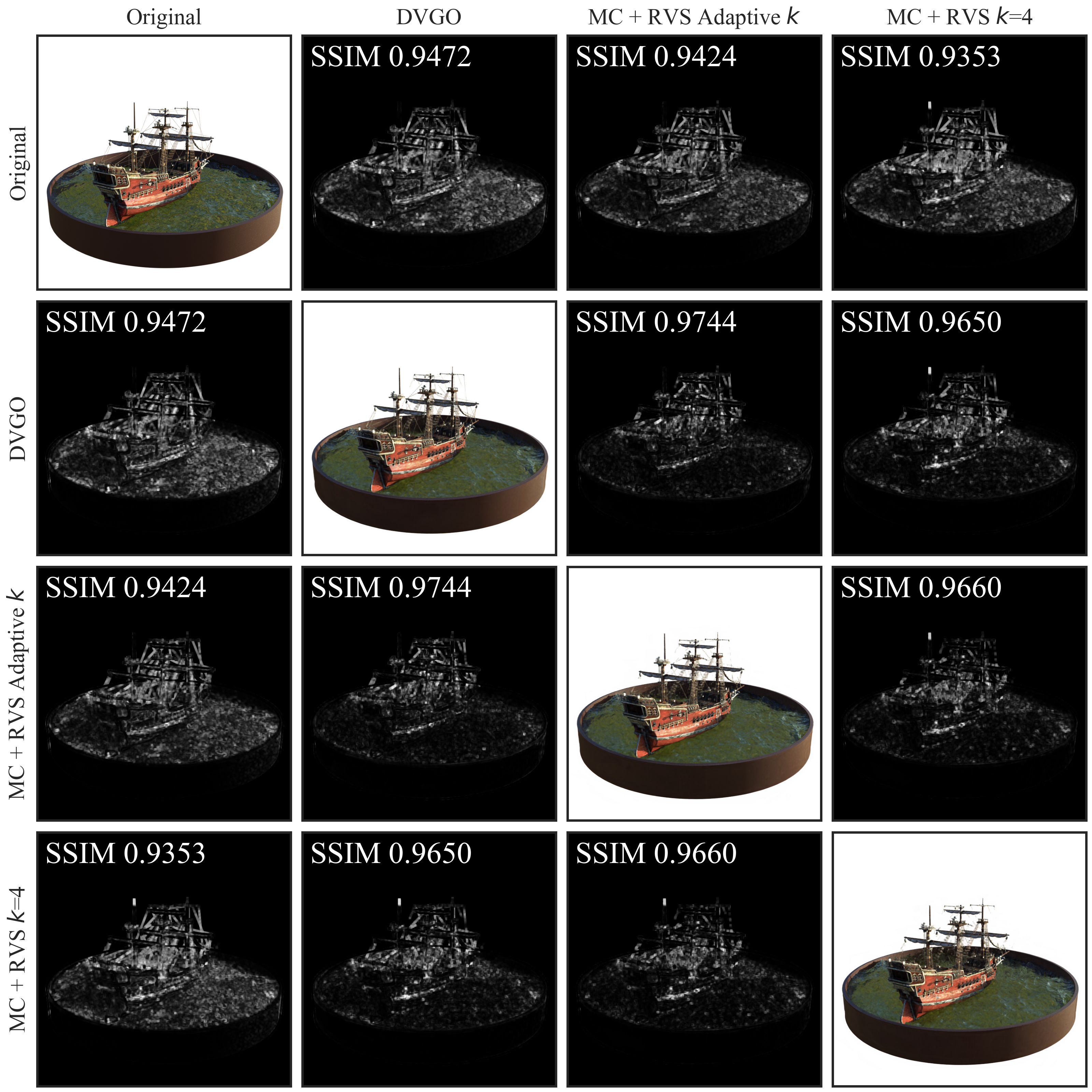
Figure 7: Qualitative comparison of scene reconstruction based on various training approaches. We visualize the default DVGO model along with two models trained using the reparameterized volume sampling algorithm (with the adaptive number of samples and $k=4$ samples). In all three models, the novel view does noes faithfully capture the water surface and fine ship details. Noticeably, the three model align in water surface reconstruction as opposed to the ship details. Perceptual quality of the details follows the numerical results.

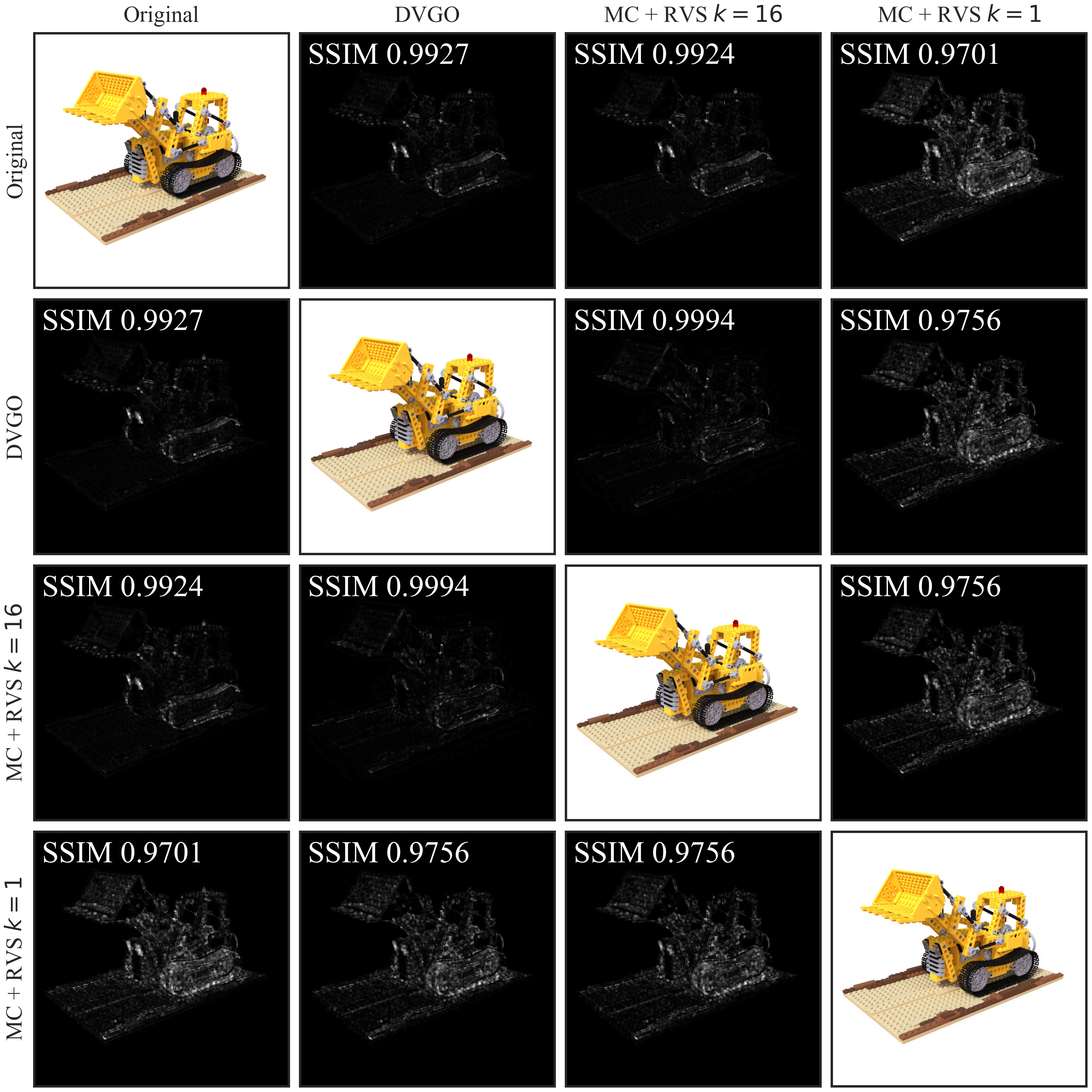
Figure 8: Comparison of novel views produced by different rendering algorithms. We trained a base DVGO model and rendered novel views using the default rendering algorithm and the proposed algorithm with $k=1,16$ samples. Except for a single-sample estimate, the rendered images on diagonal are barely distinguishable. Outside the diagonal, we visualize the difference with SSIM gradients and report SSIM between the images. The images produced with the default rendering algorithm and our algorithm with $k=16$ differ the least, whereas the image with $k$ samples has noticeable flaws near the track and edges.

Appendix E Per-Scene Results

Table 10: Differentiable hierarchical sampling with NeRF on Blender dataset.

PSNR$\uparrow$	Chair	Drums	Ficus	Hotdog	Lego	Materials	Mic	Ship	Avg
NeRF, $(N_{p}=32,N_{f}=64)$	31.33	23.89	28.26	35.44	30.11	28.65	31.46	26.76	29.49
RVS, $(N_{p}=32,N_{f}=64)$	31.99	24.60	29.27	36.18	31.89	29.31	31.84	27.19	30.26

SSIM$\uparrow$	Chair	Drums	Ficus	Hotdog	Lego	Materials	Mic	Ship	Avg
NeRF, $(N_{p}=32,N_{f}=64)$	0.956	0.908	0.949	0.972	0.947	0.940	0.973	0.834	0.934
RVS, $(N_{p}=32,N_{f}=64)$	0.958	0.915	0.955	0.974	0.955	0.946	0.974	0.834	0.939

LPIPS$\downarrow$	Chair	Drums	Ficus	Hotdog	Lego	Materials	Mic	Ship	Avg
NeRF, $(N_{p}=32,N_{f}=64)$	0.059	0.116	0.063	0.050	0.070	0.072	0.033	0.220	0.085
RVS, $(N_{p}=32,N_{f}=64)$	0.056	0.113	0.060	0.050	0.066	0.065	0.033	0.219	0.082

Table 11: Differentiable hierarchical sampling with NeRF on LLFF dataset.

PSNR$\uparrow$	Room	Fern	Leaves	Fortress	Orchids	Flower	T-Rex	Horns	Avg
NeRF, $(N_{p}=32,N_{f}=64)$	31.22	24.79	20.81	31.00	20.32	27.41	25.89	26.64	26.01
RVS, $(N_{p}=32,N_{f}=64)$	31.87	24.89	20.89	31.11	20.27	27.40	26.48	26.98	26.24

SSIM$\uparrow$	Room	Fern	Leaves	Fortress	Orchids	Flower	T-Rex	Horns	Avg
NeRF, $(N_{p}=32,N_{f}=64)$	0.938	0.771	0.678	0.875	0.630	0.822	0.858	0.798	0.796
RVS, $(N_{p}=32,N_{f}=64)$	0.942	0.773	0.681	0.878	0.630	0.823	0.869	0.795	0.799

LPIPS$\downarrow$	Room	Fern	Leaves	Fortress	Orchids	Flower	T-Rex	Horns	Avg
NeRF, $(N_{p}=32,N_{f}=64)$	0.203	0.309	0.328	0.187	0.338	0.226	0.279	0.310	0.273
RVS, $(N_{p}=32,N_{f}=64)$	0.193	0.310	0.328	0.182	0.340	0.223	0.267	0.311	0.270

Table 12: Differentiable hierarchical sampling with NeRF++ on LF dataset.

PSNR$\uparrow$	Africa	Basket	Torch	Ship	Avg
NeRF++, $(N_{p}=32,N_{f}=64)$	26.36	21.38	23.72	24.53	23.99
RVS, $(N_{p}=32,N_{f}=64)$	27.31	21.58	24.60	25.01	24.63

SSIM$\uparrow$	Africa	Basket	Torch	Ship	Avg
NeRF++, $(N_{p}=32,N_{f}=64)$	0.838	0.790	0.767	0.744	0.784
RVS, $(N_{p}=32,N_{f}=64)$	0.865	0.812	0.797	0.777	0.812

LPIPS$\downarrow$	Africa	Basket	Torch	Ship	Avg
NeRF++, $(N_{p}=32,N_{f}=64)$	0.221	0.302	0.297	0.329	0.287
RVS, $(N_{p}=32,N_{f}=64)$	0.177	0.290	0.258	0.288	0.253

Table 13: Differentiable hierarchical sampling with NeRF++ on T&T dataset.

PSNR$\uparrow$	Truck	Train	M60	Playground	Avg
NeRF++, $(N_{p}=32,N_{f}=64)$	21.18	17.16	16.96	21.55	19.21
RVS, $(N_{p}=32,N_{f}=64)$	21.62	17.32	17.48	22.05	19.62

SSIM$\uparrow$	Truck	Train	M60	Playground	Avg
NeRF++, $(N_{p}=32,N_{f}=64)$	0.661	0.539	0.617	0.633	0.612
RVS, $(N_{p}=32,N_{f}=64)$	0.666	0.545	0.619	0.657	0.622

LPIPS$\downarrow$	Truck	Train	M60	Playground	Avg
NeRF++, $(N_{p}=32,N_{f}=64)$	0.423	0.541	0.516	0.493	0.493
RVS, $(N_{p}=32,N_{f}=64)$	0.410	0.527	0.506	0.446	0.472

Table 14: DVGO with Monte Carlo estimates on Blender dataset.

PSNR$\uparrow$	Chair	Drums	Ficus	Hotdog	Lego	Materials	Mic	Ship	Avg
DVGO	34.07	25.40	32.59	36.75	34.64	29.58	33.14	29.02	31.90
MC + RVS, $k=4$	33.79	25.16	31.81	36.22	33.35	28.32	33.03	27.87	31.19
MC + RVS, $k=8$	33.49	25.16	31.30	36.26	33.34	28.64	32.87	27.99	31.13
MC + RVS, adaptive $k$	34.13	25.18	31.17	36.63	33.85	29.09	33.03	28.43	31.44

SSIM$\uparrow$	Chair	Drums	Ficus	Hotdog	Lego	Materials	Mic	Ship	Avg
DVGO	0.976	0.929	0.977	0.980	0.976	0.950	0.983	0.877	0.956
MC + RVS, $k=4$	0.976	0.927	0.975	0.979	0.971	0.938	0.982	0.857	0.951
MC + RVS, $k=8$	0.973	0.927	0.972	0.979	0.970	0.942	0.981	0.861	0.951
MC + RVS, adaptive $k$	0.977	0.928	0.972	0.980	0.973	0.946	0.982	0.870	0.953

LPIPS$\downarrow$	Chair	Drums	Ficus	Hotdog	Lego	Materials	Mic	Ship	Avg
DVGO	0.028	0.080	0.025	0.034	0.027	0.058	0.018	0.162	0.054
MC + RVS, $k=4$	0.028	0.079	0.028	0.038	0.032	0.070	0.017	0.181	0.059
MC + RVS, $k=8$	0.031	0.080	0.030	0.037	0.033	0.067	0.019	0.178	0.059
MC + RVS, adaptive $k$	0.027	0.081	0.031	0.034	0.031	0.062	0.019	0.165	0.056

References

- [1] Relja Arandjelović and Andrew Zisserman, ‘Nerf in detail: Learning to sample for view synthesis’, arXiv preprint arXiv:2106.05264, (2021).
- [2] Jonathan T Barron, Ben Mildenhall, Matthew Tancik, Peter Hedman, Ricardo Martin-Brualla, and Pratul P Srinivasan, ‘Mip-nerf: A multiscale representation for anti-aliasing neural radiance fields’, in Proceedings of the IEEE/CVF International Conference on Computer Vision, pp. 5855–5864, (2021).
- [3] Jonathan T Barron, Ben Mildenhall, Dor Verbin, Pratul P Srinivasan, and Peter Hedman, ‘Mip-nerf 360: Unbounded anti-aliased neural radiance fields’, in Proceedings of the IEEE/CVF Conference on Computer Vision and Pattern Recognition, pp. 5470–5479, (2022).
- [4] Jonathan T Barron, Ben Mildenhall, Dor Verbin, Pratul P Srinivasan, and Peter Hedman, ‘Zip-nerf: Anti-aliased grid-based neural radiance fields’, arXiv preprint arXiv:2304.06706, (2023).
- [5] Charles Blundell, Julien Cornebise, Koray Kavukcuoglu, and Daan Wierstra, ‘Weight uncertainty in neural network’, in International conference on machine learning, pp. 1613–1622. PMLR, (2015).
- [6] Anpei Chen, Zexiang Xu, Andreas Geiger, Jingyi Yu, and Hao Su, ‘Tensorf: Tensorial radiance fields’, in Computer Vision–ECCV 2022: 17th European Conference, Tel Aviv, Israel, October 23–27, 2022, Proceedings, Part XXXII, pp. 333–350. Springer, (2022).
- [7] Jiemin Fang, Lingxi Xie, Xinggang Wang, Xiaopeng Zhang, Wenyu Liu, and Qi Tian, ‘Neusample: Neural sample field for efficient view synthesis’, arXiv preprint arXiv:2111.15552, (2021).
- [8] Mikhail Figurnov, Shakir Mohamed, and Andriy Mnih, ‘Implicit reparameterization gradients’, Advances in Neural Information Processing Systems, 31, (2018).
- [9] Sara Fridovich-Keil, Alex Yu, Matthew Tancik, Qinhong Chen, Benjamin Recht, and Angjoo Kanazawa, ‘Plenoxels: Radiance fields without neural networks’, in Proceedings of the IEEE/CVF Conference on Computer Vision and Pattern Recognition, pp. 5501–5510, (2022).
- [10] Yarin Gal and Zoubin Ghahramani, ‘Dropout as a bayesian approximation: Representing model uncertainty in deep learning’, in international conference on machine learning, pp. 1050–1059. PMLR, (2016).
- [11] Stephan J Garbin, Marek Kowalski, Matthew Johnson, Jamie Shotton, and Julien Valentin, ‘Fastnerf: High-fidelity neural rendering at 200fps’, in Proceedings of the IEEE/CVF International Conference on Computer Vision, pp. 14346–14355, (2021).
- [12] Peter Hedman, Pratul P Srinivasan, Ben Mildenhall, Jonathan T Barron, and Paul Debevec, ‘Baking neural radiance fields for real-time view synthesis’, in Proceedings of the IEEE/CVF International Conference on Computer Vision, pp. 5875–5884, (2021).
- [13] Tao Hu, Shu Liu, Yilun Chen, Tiancheng Shen, and Jiaya Jia, ‘Efficientnerf efficient neural radiance fields’, in Proceedings of the IEEE/CVF Conference on Computer Vision and Pattern Recognition, pp. 12902–12911, (2022).
- [14] Diederik P Kingma and Jimmy Ba, ‘Adam: A method for stochastic optimization’, arXiv preprint arXiv:1412.6980, (2014).
- [15] Diederik P Kingma and Max Welling, ‘Auto-encoding variational bayes’, arXiv preprint arXiv:1312.6114, (2013).
- [16] Andreas Kurz, Thomas Neff, Zhaoyang Lv, Michael Zollhöfer, and Markus Steinberger, ‘Adanerf: Adaptive sampling for real-time rendering of neural radiance fields’, in Computer Vision–ECCV 2022: 17th European Conference, Tel Aviv, Israel, October 23–27, 2022, Proceedings, Part XVII, pp. 254–270. Springer, (2022).
- [17] Marc Levoy, ‘Efficient ray tracing of volume data’, ACM Transactions on Graphics (TOG), 9(3), 245–261, (1990).
- [18] Ruilong Li, Matthew Tancik, and Angjoo Kanazawa, ‘Nerfacc: A general nerf acceleration toolbox’, arXiv preprint arXiv:2210.04847, (2022).
- [19] David B Lindell, Julien NP Martel, and Gordon Wetzstein, ‘Autoint: Automatic integration for fast neural volume rendering’, in Proceedings of the IEEE/CVF Conference on Computer Vision and Pattern Recognition, pp. 14556–14565, (2021).
- [20] Lingjie Liu, Jiatao Gu, Kyaw Zaw Lin, Tat-Seng Chua, and Christian Theobalt, ‘Neural sparse voxel fields’, Advances in Neural Information Processing Systems, 33, 15651–15663, (2020).
- [21] Guillaume Loubet, Nicolas Holzschuch, and Wenzel Jakob, ‘Reparameterizing discontinuous integrands for differentiable rendering’, ACM Transactions on Graphics (TOG), 38(6), 1–14, (2019).
- [22] Nelson Max, ‘Optical models for direct volume rendering’, IEEE Transactions on Visualization and Computer Graphics, 1(2), 99–108, (1995).
- [23] Ben Mildenhall, Pratul P Srinivasan, Rodrigo Ortiz-Cayon, Nima Khademi Kalantari, Ravi Ramamoorthi, Ren Ng, and Abhishek Kar, ‘Local light field fusion: Practical view synthesis with prescriptive sampling guidelines’, ACM Transactions on Graphics (TOG), 38(4), 1–14, (2019).
- [24] Ben Mildenhall, Pratul P Srinivasan, Matthew Tancik, Jonathan T Barron, Ravi Ramamoorthi, and Ren Ng, ‘Nerf: Representing scenes as neural radiance fields for view synthesis’, in European conference on computer vision, pp. 405–421. Springer, (2020).
- [25] Shakir Mohamed, Mihaela Rosca, Michael Figurnov, and Andriy Mnih, ‘Monte carlo gradient estimation in machine learning.’, J. Mach. Learn. Res., 21(132), 1–62, (2020).
- [26] Dmitry Molchanov, Arsenii Ashukha, and Dmitry Vetrov, ‘Variational dropout sparsifies deep neural networks’, in International Conference on Machine Learning, pp. 2498–2507. PMLR, (2017).
- [27] Thomas Müller, Alex Evans, Christoph Schied, and Alexander Keller, ‘Instant neural graphics primitives with a multiresolution hash encoding’, ACM Trans. Graph., 41(4), 102:1–102:15, (July 2022).
- [28] Thomas Neff, Pascal Stadlbauer, Mathias Parger, Andreas Kurz, Joerg H Mueller, Chakravarty R Alla Chaitanya, Anton Kaplanyan, and Markus Steinberger, ‘Donerf: Towards real-time rendering of compact neural radiance fields using depth oracle networks’, in Computer Graphics Forum, volume 40, pp. 45–59. Wiley Online Library, (2021).
- [29] Martin Piala and Ronald Clark, ‘Terminerf: Ray termination prediction for efficient neural rendering’, in 2021 International Conference on 3D Vision (3DV), pp. 1106–1114. IEEE, (2021).
- [30] Daniel Rebain, Wei Jiang, Soroosh Yazdani, Ke Li, Kwang Moo Yi, and Andrea Tagliasacchi, ‘Derf: Decomposed radiance fields’, in Proceedings of the IEEE/CVF Conference on Computer Vision and Pattern Recognition, pp. 14153–14161, (2021).
- [31] Christian Reiser, Songyou Peng, Yiyi Liao, and Andreas Geiger, ‘Kilonerf: Speeding up neural radiance fields with thousands of tiny mlps’, in Proceedings of the IEEE/CVF International Conference on Computer Vision, pp. 14335–14345, (2021).
- [32] Danilo Jimenez Rezende, Shakir Mohamed, and Daan Wierstra, ‘Stochastic backpropagation and approximate inference in deep generative models’, in International conference on machine learning, pp. 1278–1286. PMLR, (2014).
- [33] Cheng Sun, Min Sun, and Hwann-Tzong Chen, ‘Direct voxel grid optimization: Super-fast convergence for radiance fields reconstruction’, arXiv preprint arXiv:2111.11215, (2021).
- [34] Matthew Tancik, Pratul Srinivasan, Ben Mildenhall, Sara Fridovich-Keil, Nithin Raghavan, Utkarsh Singhal, Ravi Ramamoorthi, Jonathan Barron, and Ren Ng, ‘Fourier features let networks learn high frequency functions in low dimensional domains’, Advances in Neural Information Processing Systems, 33, 7537–7547, (2020).
- [35] Lin Yen-Chen. Nerf-pytorch. https://github.com/yenchenlin/nerf-pytorch/, 2020.
- [36] Alex Yu, Sara Fridovich-Keil, Matthew Tancik, Qinhong Chen, Benjamin Recht, and Angjoo Kanazawa, ‘Plenoxels: Radiance fields without neural networks’, arXiv preprint arXiv:2112.05131, (2021).
- [37] Alex Yu, Ruilong Li, Matthew Tancik, Hao Li, Ren Ng, and Angjoo Kanazawa, ‘Plenoctrees for real-time rendering of neural radiance fields’, in Proceedings of the IEEE/CVF International Conference on Computer Vision, pp. 5752–5761, (2021).
- [38] Kai Zhang, Gernot Riegler, Noah Snavely, and Vladlen Koltun, ‘Nerf++: Analyzing and improving neural radiance fields’, arXiv preprint arXiv:2010.07492, (2020).