Dirac bracket and time dependent constraints

Abstract

We provide a compact derivation of the Dirac bracket and of the equations of motion for second class constrained systems when the constraints are time dependent. The examples of Parameterized Mechanics and of General Relativity after gauge fixing are given, and the need for the use of time dependent gauge fixing conditions in these examples is illustrated geometrically.

Constrained systems play a major role in Modern Physics, most notably in gauge theories and in General Relativity. Dirac set up a recipe for the canonical quantization of constrained systems, introducing a new bracket, today known as Dirac bracket, which satisfies all properties desirable for a Poisson bracket (linearity in both arguments, Leibnitz rule, antisymmetry and the Jacobi identity), and which preserves the form of Hamilton’s equations of motion when written in terms of brackets.

In the case of pure gauge theories, gauge-fixing conditions which are time independent can be set, but in the case of diffeomorphism invariant theories, the gauge fixing conditions have to be time dependent. In Dirac’s original work the Hamiltonian and the constraints are time independent. The case of time dependent constraints was later treated by Mukunda in a very clear article. The purpose of the present article is to provide an alternative derivation of Mukunda’s results, and one which concomitantly provides an alternative route for the definition of the Dirac bracket.

1 Gauge-fixed constrained systems

In this section we shall not review Dirac’s method, which may be familiar to many readers and which is very clearly exposed in his original work [1] and in other works [2, 3, 4], rather we shall start from a Hamiltonian which is already in the form

$$H=H_{0}+\sum_{a=1}^{2M}u_{a}c_{a}\quad,$$ (1)

arising from Dirac’s procedure and where to each first class constraint a “gauge-fixing” constraint has been added by hand, the whole set of constraints becoming second class.

The antisymmetric matrix

$$M_{ab}=\left\{c_{a},c_{b}\right\}$$ (2)

is, by definition of second class property, non-singular,

$$\det M\neq 0\quad.$$ (3)

Dirac showed that the second class constraints can be set strongly to zero, as long as, in all relevant physical equations, the Poisson bracket is replaced by the new bracket (Dirac bracket)

$$\left\{F,G\right\}_{D}=\left\{F,G\right\}-\left\{F,c_{a}\right\}M_{ab}^{-1}\left\{c_{b},G\right\}\quad,$$ (4)

where summation over repeated indices is understood, and that the evolution of a phase space variable is given by

$$\dot{F}=\left\{F,H_{0}\right\}_{D}+\frac{\partial F}{\partial t}\quad.$$ (5)

Mukunda [5] showed that, in the presence of time dependent constraints, equation (5) should be replaced by

$$\dot{F}=\left\{F,H_{0}\right\}_{D}+\left(\frac{\partial F}{\partial t}\right)_{D}\quad,$$ (6)

with

$$\left(\frac{\partial F}{\partial t}\right)_{D}=\frac{\partial F}{\partial t}-\left\{F,c_{a}\right\}M_{ab}^{-1}\frac{\partial c_{b}}{\partial t}\quad.$$ (7)

2 Parameterized Mechanics

We consider the example of a theory describable by an action principle, from an action

$$S=\int_{t_{1}}^{t_{2}}\mathcal{L}\left(x^{\mu},\dot{x}^{\mu}\right)dt$$ (8)

which is invariant under redefinitions of the evolution parameter,

$$t\rightarrow f\left(t\right)\quad.$$ (9)

This is a diffeomorphism invariant theory in one dimension. We use the calligraphic letter $\mathcal{L}$ to denote the Lagrangian while reserving the capital letter $L$ to denote another function, for reasons to become clear below.

The Lagrangian $\mathcal{L}$ cannot depend explicitly on $t$ and it must be homogeneous of the first kind in the derivatives of the velocities [1, 4],

$$\mathcal{L}\left(x^{\mu},\lambda\dot{x}^{\mu}\right)=\lambda\mathcal{L}\left(x^{\mu},\dot{x}^{\mu}\right)\quad,$$ (10)

with $\mu=0,\ldots,d$. Moreover, if we assume that one of the configuration space variables, $x^{0}$, is a monotonous function of time, $dx^{0}/dt>0$, this condition can be stated as

$$\mathcal{L}\left(x^{\mu},\dot{x}^{\mu}\right)=L\left(x^{0},x^{i},\frac{\dot{x}^{i}}{\dot{x}^{0}}\right)\dot{x}^{0}\quad,$$ (11)

with $i=1,\ldots,d$. The momenta conjugate to the configuration space variables are

$$p^{0} = L-\frac{\partial L}{\partial\left(\dot{x}^{i}/\dot{x}^{0}\right)}\frac{\dot{x}^{i}}{\dot{x}^{0}}$$ (12)

$$p^{i} = \frac{\partial L}{\partial\left(\dot{x}^{i}/\dot{x}^{0}\right)}\quad,$$ (13)

and the Hamiltonian vanishes

$$\mathcal{H}=p^{0}\dot{x}^{0}+p^{i}\dot{x}^{i}-\mathcal{L}=0\quad.$$ (14)

Assuming that the relation (13) between the $p^{i}$ and the $\dot{x}^{i}/\dot{x}^{0}$ is invertible (if it is not, then further constraints show up - but we assume it is, in order to concentrate on the reparameterization invariance alone), one can write equation (12) in the form

$$p^{0}+H\left(x^{0},x^{i},p^{i}\right)=0\quad,$$ (15)

with

$$H=\frac{\partial L}{\partial\left(\dot{x}^{i}/\dot{x}^{0}\right)}\frac{\dot{x}^{i}}{\dot{x}^{0}}-L\quad,$$ (16)

which is clearly recognizable as the Legendre transform of $L$ in the variables $\dot{x}^{i}/\dot{x}^{0}$, that is, the Hamiltonian associated with the function $L$, seen as a Lagrangian. This is why we reserved the calligraphic letters $\mathcal{L}$ and $\mathcal{H}$ for the original Lagrangian and Hamiltonian of the theory.

Equation (15) is a constraint and, because we assumed (13) to be invertible, it is the only constraint, hence a first order one. Therefore the time evolution is undetermined, which we should have expected because we have the freedom to choose any parameterization that we want for the evolution variable $t$.

In order to have a well determined time evolution, one needs to fix the gauge, and adding the constraint $x^{0}=0$ to (15) seems to be a good choice, because $\left\{x^{0},p^{0}+H\left(x^{0},x^{i},p^{i}\right)\right\}=1$. However, the hamiltonian vanishes strongly, $\mathcal{H}=0$, and using (5) one would get $\dot{F}\left(x^{\mu},p^{\mu}\right)=0$ for any function in phase space: there would be no dynamics!

The problem is that the transformation (9) that leaves the action (8) invariant is not a pure gauge transformation in the sense that the transformation is not among the phase space variables only, rather involving the evolution parameter. While for pure gauge transformations, gauge fixing conditions that involve only phase space variables can be used, in the case of the invariance under reparameterizations of the evolution variable, the “gauge fixing” conditions must necessarily involve the evolution variable itself, since that is the variable that must be fixed.

This is ilustrated in figure 1. On the left hand side of the figure is an example where the variable $x^{0}$ is pure gauge ($x^{1}$ is some other variable, added for illustrative purposes - it may be looked upon as the rest of phase space), that is, the system is invariant under $x^{0}\rightarrow x^{0}+\alpha$, and on the right hand side of the figure is an example where the system is invariant under reparameterizations $t\rightarrow f\left(t\right)$. In both cases, evolution is undetermined, with dotted lines representing equivalent solutions. In the first case the gauge can be fixed with $x^{0}=0$. Then the solution is unique (solid line). In the second case, setting $x^{0}=0$ (first solid line) freezes the dynamics ($x^{1}=const.$), but setting $x^{0}=t$ preserves the dynamics (second solid line).

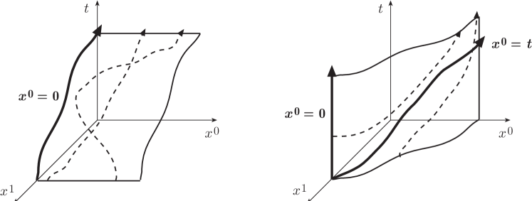
Figure 1: Left: Equivalent orbits when $x^{0}$ is pure gauge. The gauge can be fixed by setting $x^{0}=0$. Right: Equivalent orbits for invariance under reparameterization of the evolution variable $t$. Setting $x^{0}=0$ would freeze the dynamics, but setting $x^{0}=t$ is acceptable.

The examples in figure 1 also illustrate why (5) has got to be improved when the constraints are time dependent. After eliminating the variable $x^{0}$ one has

$$\left(\frac{\partial F}{\partial t}\right)_{x^{1}=cont}=\frac{\partial F}{\partial x^{0}}\frac{dx^{0}}{dt}+\frac{\partial F}{\partial t}\quad.$$ (17)

Setting $x^{0}=0$ we get

$$\left(\frac{\partial F}{\partial t}\right)_{x^{1}=cont}=\frac{\partial F}{\partial t}\quad.$$ (18)

But setting $x^{0}=t$ we get

$$\left(\frac{\partial F}{\partial t}\right)_{x^{1}=cont}=\frac{\partial F}{\partial x^{0}}+\frac{\partial F}{\partial t}\quad.$$ (19)

It is therefore the term $\partial F/\partial t$ that has got to be corrected in (5).

Back to our theory, adding instead the gauge fixing constraint

$$C\left(x^{0},x^{i},p^{i}\right)-t=0$$ (20)

to (12), with

$$\left\{C,p^{0}+H\right\}\neq 0\quad,$$ (21)

one gets, using (6) and (7) instead of, (5)

$$\dot{F}=\frac{\partial F}{\partial t}+\frac{\left\{F,p^{0}+H\right\}}{\left\{C,p^{0}+H\right\}}\quad.$$ (22)

As for the quantization of the theory, since $\mathcal{H}=0$ there is no immediate Schrödinger picture, but the system can be described in the Heisenberg picture because one can compute $\dot{F}$ using (22).

Furthermore, after some manipulation, one arrives, starting from (22), at

$$\dot{F}=\left\{F,H\right\}_{D}+\frac{\partial F}{\partial t}+\left\{F,p^{0}\right\}+\frac{\left\{C,F\right\}\left\{p^{0},H\right\}}{\left\{C,p^{0}+H\right\}}\quad.$$ (23)

Hence, a Schrödinger picture can be recovered with hamiltonian given by $H$, once one solves the constraints: the last three terms in this equation can be interpreted as the explicit variation with respect to time. This is clear if one chooses $C=x^{0}$ and solve the constraints for $x^{0}$ and $p^{0}$. Then equation (23) reads

$$\dot{F}=\left\{F,H\right\}_{D}+\frac{\partial F}{\partial t}+\frac{\partial F}{\partial x^{0}}-\frac{\partial F}{\partial p^{0}}\frac{\partial H}{\partial x^{0}}\quad.$$

The action (8) can be obtained by the inverse procedure, starting from

$$S=\int_{x_{0(1)}}^{x_{0(2)}}L\left(x^{0},x^{i},\frac{dx^{i}}{dx^{0}}\right)dx^{0}$$

and parameterizing the variable $x^{0}=x^{0}\left(t\right)$ [1, 4]. That is why it is called Parameterized Mechanics.

3 General Relativity

General Relativity is a field theory and, as such, its treatment is more elaborate than that of Mechanics, which has a discrete number of degrees of freedom. We shall not review the extension of Analytical Mechanics to field theories - that is the reason why one ends up with a hamiltonian density (25) and why the delta functions show up in formulas (27)-(31) -, which is available elsewhere in many textbooks [4, 6], but merely illustrate what a straightforward extension of this formalism to General Relativity would look like.

Of course, the treatment of field theories involves several further complications, such as the existence or not of global gauge fixing conditions, the presence of surface terms, etc. (for a review of many of these matters see [7] or [8]). We shall not deal with these issues as the example of General Relativity serves here merely the purpose of motivation for the subject at hand.

The action for General Relativity can be written in the form

$$S=\int dt\int d^{3}x\left(\frac{1}{2}\pi^{ij}\dot{g}_{ij}-NH-N^{i}P_{i}\right)\quad,$$ (24)

where $H$ and $P_{i}$ are functions of the space-space components of the metric $g_{ij}$ and their conjugate momenta $\pi^{ij}$ and $N$ and $N^{i}$ are functions that involve the space-time and time-time components of the metric. Since the time derivatives of these latest components of the metric do not show up in the action, the function $N$ and the vector $N^{i}$, called respectively the lapse and the shift, act as Lagrange multipliers for the constraints $H$ and $H_{i}$, called respectively the hamiltonian constraint and the momentum constraints. This is the so-called ADM decomposition of the action [7].

Therefore General Relativity is a totally constrained theory, its hamiltonian density being a combination of four constraints, which, for convenience, we shall label in four-vector notation,

$$\mathcal{H}\left(x\right)=N_{\mu}P^{\mu}\quad.$$ (25)

These four constraints arise from the invariance under the four-dimensional (per point) group of diffeomorphisms in four dimensions, and they turn out to be first class. Since the space-space part of the metric has got six independent components, one arrives at the well-known counting of $6-4=2$ degrees of freedom per point for General Relativity.

One way to fix the gauge is to add four extra constraints

$$C^{\alpha}\left(x\right)=X^{\alpha}\left[\pi^{ij},g_{ij}\right]-x^{\alpha}=0$$ (26)

to the existing four $P^{\mu}$. Here $X^{\alpha}$ is some function of the canonical variables at the point $x$. This can be interpreted as choosing a coordinate system [1, 7, 8, 9]. Indeed the original constraints of the theory arise precisely because of the freedom to choose the coordinate system.

The eight constraints $P^{\mu}$ and $C^{\alpha}$ have a matrix of Poisson brackets with the form

$$M\left(\vec{x},\vec{y},t\right)=\left[\begin{array}[]{cc}D&-\Lambda\\ \Lambda^{T}&0\end{array}\right]\delta^{3}\left(\vec{x}-\vec{y}\right)\quad,$$ (27)

where

$$D^{\alpha\beta}\left(\vec{x},t\right)\delta^{3}\left(\vec{x}-\vec{y}\right)=\left\{X^{\alpha}\left(\vec{x},t\right),X^{\beta}\left(\vec{y},t\right)\right\}$$ (28)

$$\Lambda^{\mu\beta}\left(\vec{x},t\right)\delta^{3}\left(\vec{x}-\vec{y}\right)=-\left\{P^{\mu}\left(\vec{x},t\right),X^{\beta}\left(\vec{y},t\right)\right\}$$ (29)

$$0=\left\{P^{\mu}\left(\vec{x},t\right),P^{\nu}\left(\vec{y},t\right)\right\}\quad.$$ (30)

The last equality follows from the first order nature of the hamiltonian and the momentum constraints.

One has (see [4] for the subtleties involved in the construction of the inverse)

$$M^{-1}\left(\vec{x},\vec{y},t\right)=\left[\begin{array}[]{cc}0&\left(\Lambda^{-1}\right)^{T}\\ -\Lambda^{-1}&\Lambda^{-1}D\left(\Lambda^{-1}\right)^{T}\end{array}\right]\delta^{3}\left(\vec{x}-\vec{y}\right)\quad,$$ (31)

and the condition that must be satisfied for the correct fixing of the gauge is that

$$\det\left(\Lambda\right)\neq 0\quad.$$ (32)

Then it results from (6) and (7) - in their extension to field theories - that

$$\dot{F}=\int d^{3}x\left\{F,P^{\mu}\left(\vec{x},t\right)\right\}\Lambda_{\mu 0}^{-1}\left(\vec{x},t\right)\quad.$$ (33)

Hence, General Relativity could be quantized “in principle” in the Heisenberg picture using (33) and the Dirac bracket

$$\left\{F,G\right\}_{D} = \left\{F,G\right\}-\int d^{3}x\left\{F,P^{\mu}\right\}\Lambda_{\mu\rho}^{-1}D^{\rho\sigma}\Lambda_{\nu\sigma}^{-1}\left\{P^{\nu},G\right\}-$$

$$-\int d^{3}x\left\{G,P^{\mu}\right\}\Lambda_{\mu\beta}^{-1}\left\{X^{\beta},F\right\}+\int d^{3}x\left\{F,P^{\mu}\right\}\Lambda_{\mu\beta}^{-1}\left\{X^{\beta},G\right\}$$

The issue of solving the constraints and writing (33) in the form of a bracket of $F$ with a certain Hamiltonian $H$ and passing to a Schrödinger picture is discussed in [7] and is closely related to the issue of definition of energy in General Relativity.

The purpose of this section was to show the relevance of the topic of this article to the very important subject of General Relativity, and in fact to diffeomorphism invariant theories in general. For a detailed list of all the details involved see [1, 4, 7, 8, 9]. In the remaining sections we proceed to the main point of the article, which is to provide a compact derivation of (6), (4) and (7).

4 Time dependent constraints

We shall use the notation in [10], which we find more practical for the present purpose. In this notation, the set of canonical coordinates $x_{i}$ and $p_{i}$ is composed into a column vector, and the same is done for the derivatives of a function $F$ with respect to the canonical variables,

$$\eta=\left[\begin{array}[]{c}x_{1}\\ \cdots\\ x_{N}\\ p_{1}\\ \cdots\\ p_{N}\end{array}\right]\quad\quad\frac{\partial F}{\partial\eta}=\left[\begin{array}[]{c}\partial F/\partial x_{1}\\ \cdots\\ \partial F/\partial x_{N}\\ \partial F/\partial p_{1}\\ \cdots\\ \partial F/\partial p_{N}\end{array}\right]\quad.$$ (35)

With the help of the matrix

$$\mathbf{J}=\left[\begin{array}[]{cc}0&1_{N\times N}\\ -1_{N\times N}&0\end{array}\right]\quad,$$ (36)

Hamilton’s equations of motion can be succinctly written as

$$\dot{\eta}=\mathbf{J}\frac{\partial H}{\partial\eta}\quad,$$ (37)

with $H$ the Hamiltonian. The Poisson bracket between two functions $F$ and $G$ becomes

$$\left\{F,G\right\}=\left(\frac{\partial F}{\partial\eta}\right)^{T}\mathbf{J}\frac{\partial G}{\partial\eta}$$ (38)

and the time evolution of an arbitrary function $F$ is

$$\dot{F}=\left\{F,H\right\}+\frac{\partial F}{\partial t}\quad.$$ (39)

5 Constraint analysis

Let us now admit that the Hamiltonian contains $2M$ second-class constraints $c_{a}$ which we write in the form of a column vector too

$$c\left(\eta,t\right)=0\quad.$$ (40)

Its time derivative is

$$\dot{c}=\mathbf{C}\dot{\eta}+\frac{\partial c}{\partial t}=0\quad.$$ (41)

It must vanish, as the constraints are to be maintained with evolution. Here we have defined the $2M\times 2N$ matrix

$$C_{ai}=\frac{\partial c_{a}}{\partial\eta_{i}}\quad.$$ (42)

Equation (41) is a simple linear equation. It admits a solution if and only if [11]

$$\left(\mathbf{1}-\mathbf{CC}^{-1}\right)\frac{\partial c}{\partial t}=0\quad,$$ (43)

where $\mathbf{C}^{-1}$ is a pseudoinverse of $\mathbf{C}$, that is, a $2N\times 2M$ matrix satisfying

$$\mathbf{CC}^{-1}\mathbf{C=C}\quad.$$

Its solution is [11]

$$\dot{\eta}=\left(\mathbf{1}-\mathbf{C}^{-1}\mathbf{C}\right)Z-\mathbf{C}^{-1}\frac{\partial c}{\partial t}\quad,$$ (44)

for some $Z$. Since we know that in the absence of constraints (37) holds, one must have

$$Z=\mathbf{J}\frac{\partial H}{\partial\eta}\quad.$$ (45)

Hence

$$\dot{\eta}=\left(\mathbf{1}-\mathbf{C}^{-1}\mathbf{C}\right)\mathbf{J}\frac{\partial H}{\partial\eta}-\mathbf{C}^{-1}\frac{\partial c}{\partial t}\quad.$$ (46)

Now we can compute the total derivative of a function $F\left(\eta,t\right)$

$$\dot{F} = \left(\frac{\partial F}{\partial\eta}\right)^{T}\dot{\eta}+\frac{\partial F}{\partial t}=$$ (47)

$$= \left(\frac{\partial F}{\partial\eta}\right)^{T}\left(\mathbf{1}-\mathbf{C}^{-1}\mathbf{C}\right)\mathbf{J}\frac{\partial H}{\partial\eta}-\left(\frac{\partial F}{\partial\eta}\right)^{T}\mathbf{C}^{-1}\frac{\partial c}{\partial t}+\frac{\partial F}{\partial t}=$$

$$= \left(\frac{\partial F}{\partial\eta}\right)^{T}\mathbf{J}\frac{\partial H}{\partial\eta}-\left(\frac{\partial F}{\partial\eta}\right)^{T}\mathbf{C}^{-1}\mathbf{CJ}\frac{\partial H}{\partial\eta}+\frac{\partial F}{\partial t}-\left(\frac{\partial F}{\partial\eta}\right)^{T}\mathbf{C}^{-1}\frac{\partial c}{\partial t}$$

We want to rewrite this equation in the form

$$\dot{F}=\left\{F,H\right\}_{D}+\left(\frac{\partial F}{\partial t}\right)_{D}$$ (48)

with a new “Poisson bracket” $\left\{F,H\right\}_{D}$ that depends linearly on $F$ and $H$, and a new “partial derivative with respect to time” $\left(\partial F/\partial t\right)_{D}$ which is linear in $F$. Then we must have

$$\left\{F,G\right\}_{D} = \left\{F,G\right\}-\left(\frac{\partial F}{\partial\eta}\right)^{T}\mathbf{C}^{-1}\mathbf{CJ}\frac{\partial G}{\partial\eta}$$ (49)

$$\left(\frac{\partial F}{\partial t}\right)_{D} = \frac{\partial F}{\partial t}-\left(\frac{\partial F}{\partial\eta}\right)^{T}\mathbf{C}^{-1}\frac{\partial c}{\partial t}\quad.$$ (50)

We have not yet determined the pseudoinverse $\mathbf{C}^{-1}$ (recall that the pseudoinverse is not unique) neither have we showed that (43) holds. Because $\mathbf{C}$ has maximal rank (otherwise the constraints would not be independent), $\mathbf{CC}^{T}$ is invertible and $\mathbf{C}^{T}\left(\mathbf{CC}^{T}\right)^{-1}$ is a pseudoinverse (in fact, a right pseudoinverse - and the Moore-Penrose pseudoinverse). This shows that (43) holds. However, using this pseudoinverse would make the Dirac bracket fail the requirement of antisymmetry under the exchange of $F$ with $G$. As we shall see, imposing this further requirement singles out one pseudoinverse.

The first parcel in (49) is certainly antisymmetric because it is the Poisson bracket. It is therefore enough to require antisymmetry for the second parcel in (49),

$$\left(\frac{\partial F}{\partial\eta}\right)^{T}\mathbf{C}^{-1}\mathbf{CJ}\frac{\partial G}{\partial\eta}=-\left(\frac{\partial G}{\partial\eta}\right)^{T}\mathbf{C}^{-1}\mathbf{CJ}\frac{\partial F}{\partial\eta}=$$

$$=-\left[\left(\frac{\partial G}{\partial\eta}\right)^{T}\mathbf{C}^{-1}\mathbf{CJ}\frac{\partial F}{\partial\eta}\right]^{T}=-\left(\frac{\partial F}{\partial\eta}\right)^{T}\mathbf{J}^{T}\left(\mathbf{C}^{-1}\mathbf{C}\right)^{T}\frac{\partial G}{\partial\eta}\quad.$$ (51)

This can only be satisfied for all $F$ and $G$ if (notice that $\mathbf{J}^{T}=-\mathbf{J}$)

$$\mathbf{C}^{-1}\mathbf{CJ}=\mathbf{J}\left(\mathbf{C}^{-1}\mathbf{C}\right)^{T}\quad\Rightarrow$$

$$\Rightarrow\quad\mathbf{C}^{-1}\mathbf{CJC}^{T}=\mathbf{JC}^{T}\left(\mathbf{C}^{-1}\right)^{T}\mathbf{C}^{T}=\mathbf{J}\left(\mathbf{CC}^{-1}\mathbf{C}\right)^{T}=\mathbf{JC}^{T}\quad.$$ (52)

Since we know that

$$\mathbf{M}=\mathbf{CJC}^{T}=\frac{\partial c_{a}}{\partial\eta_{i}}J^{ij}\frac{\partial c_{b}}{\partial\eta_{j}}=\sum_{i=1}^{N}\frac{\partial c_{a}}{\partial x_{i}}\frac{\partial c_{b}}{\partial p_{i}}-\frac{\partial c_{a}}{\partial p_{i}}\frac{\partial c_{b}}{\partial x_{i}}$$ (53)

is invertible [1] we finally get

$$\mathbf{C}^{-1}=\mathbf{JC}^{T}\mathbf{M}^{-1}\quad.$$ (54)

Substitution in (49)-(50) yields

$$\left\{F,G\right\}_{D} = \left\{F,G\right\}-\left(\frac{\partial F}{\partial\eta}\right)^{T}\mathbf{JC}^{T}\mathbf{M}^{-1}\mathbf{CJ}\frac{\partial G}{\partial\eta}$$ (55)

$$\left(\frac{\partial F}{\partial t}\right)_{D} = \frac{\partial F}{\partial t}-\left(\frac{\partial F}{\partial\eta}\right)^{T}\mathbf{JC}^{T}\mathbf{M}^{-1}\frac{\partial c}{\partial t}\quad.$$ (56)

Or, back to indices notation,

$$\left\{F,G\right\}_{D} = \left\{F,G\right\}-\frac{\partial F}{\partial\eta_{i}}J_{ij}\frac{\partial c_{a}}{\partial\eta_{j}}\left[\frac{\partial c_{a}}{\partial\eta_{m}}J_{mn}\frac{\partial c_{b}}{\partial\eta_{n}}\right]^{-1}\frac{\partial c_{b}}{\partial\eta_{k}}J_{kl}\frac{\partial G}{\partial\eta_{l}}=$$ (57)

$$= \left\{F,H\right\}-\left\{F,c_{a}\right\}\left\{c_{a},c_{b}\right\}^{-1}\left\{c_{b},G\right\}$$

$$\left(\frac{\partial F}{\partial t}\right)_{D} = \frac{\partial F}{\partial t}-\frac{\partial F}{\partial\eta_{i}}J_{ij}\frac{\partial c_{a}}{\partial\eta_{j}}\left[\frac{\partial c_{a}}{\partial\eta_{m}}J_{mn}\frac{\partial c_{b}}{\partial\eta_{n}}\right]^{-1}\frac{\partial c_{b}}{\partial t}=$$ (58)

$$= \frac{\partial F}{\partial t}-\left\{F,c_{a}\right\}\left\{c_{a},c_{b}\right\}^{-1}\frac{\partial c_{b}}{\partial t}\quad.$$

To summarize our results, we showed that one can work on the constraint surface, defined by $c_{a}=0$, provided that one replaces the Poisson bracket by the Dirac bracket

$$\left\{F,G\right\}_{D}=\left\{F,G\right\}-\left\{F,c_{a}\right\}M_{ab}^{-1}\left\{c_{b},G\right\}\quad,$$ (59)

with $M_{ab}=\left\{c_{a},c_{b}\right\}$, and the partial derivative with respect to time by

$$\left(\frac{\partial F}{\partial t}\right)_{D}=\frac{\partial F}{\partial t}-\left\{F,c_{a}\right\}M_{ab}^{-1}\frac{\partial c_{b}}{\partial t}\quad.$$ (60)

We should stress that these are not new results. Equation (59) was first derived by Dirac [1] and (60) by Mukunda [5]. Here we provided a compact and alternative derivation of both.

References

• [1] Dirac P 1964  Lectures on Quantum Mechanics (Belfer Graduate School of Science, Yeshiva University)
• [2] Henneaux M 1992 Quantization of Gauge Systems (Princeton UP)
• [3] Rothe H and Rothe K 2010 Classical and Quantum Dynamics of Constrained Hamiltonian Systems (World Scientific)
• [4] Sundermeyer K 1982 Constrained Dynamics (Springer-Verlag)
• [5] Mukunda N 1980 “Time dependent constraints in classical dynamics” Phys. Scripta 21 801
• [6] Itzykson C and Zuber J 1980 Quantum Field Theory (McGraw-Hill)
• [7] Arnowitt R, Deser S and Misner C 1959 “Dynamical Structure and Definition of Energy in General Relativity” Phys. Rev. 116 1322
• [8] Isham C 1992 “Canonical Quantum Gravity and the Problem of Time” Lecture notes from the 1992 Salamanca NATO Summer School arXiv:gr-qc/9210011
• [9] Anderson E 2012 “Ch.4: The Problem of Time in Quantum Gravity”, in V. Frignanni (Ed.) Classical and Quantum Gravity: Theory, Analysis and Applications (Nova)
• [10] Goldstein H, Poole C and Safko J 2001 Classical Mechanics (Pearson)
• [11] Ben-Israel A and Greville T 2000 Generalized Inverses - Theory and Applications (Springer)