Can Learning Be Explained By Local Optimality In Low-rank Matrix Recovery?

Abstract

We explore the local landscape of low-rank matrix recovery, aiming to reconstruct a $d_{1}\times d_{2}$ matrix with rank $r$ from $m$ linear measurements, some potentially noisy. When the true rank is unknown, overestimation is common, yielding an over-parameterized model with rank $k\geq r$. Recent findings suggest that first-order methods with the robust $\ell_{1}$-loss can recover the true low-rank solution even when the rank is overestimated and measurements are noisy, implying that true solutions might emerge as local or global minima. Our paper challenges this notion, demonstrating that, under mild conditions, true solutions manifest as strict saddle points. We study two categories of low-rank matrix recovery, matrix completion and matrix sensing, both with the robust $\ell_{1}$-loss. For matrix sensing, we uncover two critical transitions. With $m$ in the range of $\max\{d_{1},d_{2}\}r\lesssim m\lesssim\max\{d_{1},d_{2}\}k$, none of the true solutions are local or global minima, but some become strict saddle points. As $m$ surpasses $\max\{d_{1},d_{2}\}k$, all true solutions become unequivocal global minima. In matrix completion, even with slight rank overestimation and mild noise, true solutions either emerge as non-critical or strict saddle points.

1 Introduction

We study the optimization landscape of low-rank matrix recovery, where the goal is to recover a matrix $X^{\star}\in\mathbb{R}^{d_{1}\times d_{2}}$ with rank $r\leq\min\{d_{1},d_{2}\}$ from $m$ linear and possibly noisy measurements:

$$\text{find}\ X^{\star}\qquad\text{such that}\qquad\mathrm{rank}(X^{\star})=r,\ \ y=\mathcal{A}(X^{\star})+\epsilon.$$

The measurement operator $\mathcal{A}:\mathbb{R}^{d_{1}\times d_{2}}\to\mathbb{R}^{m}$ is defined as $\mathcal{A}(X)=[\langle A_{1},X\rangle\ \ \dots\ \ \langle A_{m},X\rangle]^{\top}$, and $\epsilon\in\mathbb{R}^{m}$ is the additive noise vector. Low-rank matrix recovery plays a central role in many modern machine learning problems, including motion detection in video frames [BZ14], face recognition [LFL⁺14], and collaborative filtering in recommender systems [LZXZ14]. Two well-known classes of low-rank matrix recovery are matrix completion and matrix sensing. Matrix completion employs an element-wise projection as the measurement operator, whereas in matrix sensing, the measurement matrices $\{A_{i}\}_{i=1}^{m}$ are assumed to be approximately norm-preserving.

This problem is commonly solved via a factorization technique called Burer-Monteiro factorization (BM) [BM03, BM05, CLC19]. In BM, the target low-rank matrix is modeled as $X^{\star}=W^{\star}_{1}W^{\star}_{2}$, where $W^{\star}_{1}\in\mathbb{R}^{d_{1}\times k}$ and $W^{\star}_{2}\in\mathbb{R}^{k\times d_{2}}$ are unknown factors each with search rank $k$. Based on this definition, any pair of factors $(W^{\star}_{1},W^{\star}_{2})$ that satisfies $X^{\star}=W^{\star}_{1}W^{\star}_{2}$ is called a true solution. When the true rank $r$ is known and $k=r$, the problem is exactly-parameterized. The setting $k>r$ is known as the over-parameterized regime, where the true rank is unknown and over-estimated. Given this factorized model, the problem of recovering the true solution is typically formulated as follows:

$$\min_{\mathbf{W}=(W_{1},W_{2})}f_{\ell_{q}}(\mathbf{W}):=\frac{1}{m}\left\lVert y-\mathcal{A}(W_{1}W_{2})\right\rVert^{q}_{\ell_{q}}.$$ (BM)

When the true solution is symmetric and positive semi-definite, the above problem is commonly referred to as symmetric low-rank matrix recovery, where the target low-rank matrix is modeled as $X^{\star}=W^{\star}{W^{\star}}^{\top}\in\mathbb{R}^{d\times d}$ for $W^{\star}\in\mathbb{R}^{d\times k}$.

However, this strategy presents two primary challenges. First, owing to its non-convex nature, local-search algorithms may converge to local minima, falling short of achieving global optimality. Second, in the presence of noise, the solutions obtained may not coincide with the ground truth $X^{\star}$.

To address these issues, a recent line of research has shown that, in the absence of noise, different variants of BM are devoid of spurious (sub-optimal) local minima, and their global minima coincide with the ground truth $X^{\star}$. Notably, [BNS16, GLM16] showed that, when the measurements are noiseless and the search rank coincides with the true rank $k=r$, two important variants of BM, namely matrix completion and matrix sensing with $\ell_{2}$-loss, do not have spurious local minima and their global minima coincide with the ground truth. These results led to a flurry of follow-up papers, expanding these insights to the over-parameterized and noiseless regime [Zha22, Zha21, ZFZ23], as well as exactly-parameterized and noisy regime with $\ell_{1}$-loss [MF21, FS20, LZMCSV20].

Despite the extensive body of literature addressing the optimization landscape of low-rank matrix recovery, it remains elusive whether these findings can be extrapolated to situations where both over-parameterization and noisy measurements are simultaneously present. This can be attributed, in part, to the fact that in the noisy and over-parameterized regimes, the model $W_{1}W_{2}$ has the capacity to overfit to noise. In such situations, the global minimum is unlikely to correspond to the ground truth. To illustrate this point, consider the scenario where $d_{1}=d_{2}=d$ and adopt a fully over-parameterized setting where $k=d\geq r$. Under a reasonable condition on the measurement operator $\mathcal{A}$, it is easy to see that the global minimum $(W_{1},W_{2})$ aligns perfectly with the noisy measurements, yielding a zero loss, so long as $m\leq d^{2}$. In this context, if even a single measurement is tainted by noise, the true solution $X^{\star}$ and $W_{1}W_{2}$ are not equal. This indicates that, in the presence of noise and over-parameterization, it is unlikely for the global minima to coincide with the true solution.

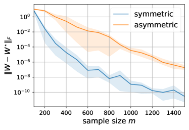
(a) Matrix sensing

(b) Matrix completion

Figure 1: When the sub-gradient method with a random and small initialization and an exponentially decaying step size is applied to the $\ell_{1}$-loss, it converges to a true solution for different types of low-rank matrix recovery problem. These problems encompass matrix sensing and matrix completion, involving both symmetric and asymmetric settings. In all of the simulations, the ground truth has dimensions $d_{1}=d_{2}=d=40$ and rank $r=2$. Moreover, the model is fully over-parameterized with a search rank of $k=40$. In the case of asymmetric matrix completion, for any instance with a sampling probability of $s<1$, the global minima perfectly overfit to noise, achieving a zero loss. A similar phenomenon occurs for asymmetric matrix sensing with sample size $m\leq 1600$.

1.1 Do True Solutions Emerge as Local Minima?

The noted observation does not inherently reject the possibility that true solutions could manifest as local minima. In fact, recent findings concerning the efficacy of local-search algorithms within the context of over-parameterized and noisy low-rank matrix recovery lend credence to this idea. For instance, a recent result showed that a simple sub-gradient method with a small initial point converges to a true solution of the symmetric matrix sensing when applied to BM with $\ell_{1}$-loss and over-parameterized rank $k>r$, provided that $m\gtrsim dr^{2}$ and at most a constant fraction of the measurements are corrupted with noise [MF23, Theorem 1]. Surprisingly, this result holds even in the over-parameterized regime where $m=\Theta(dr^{2})\ll dk$—in such scenarios, the global minima overfit to noise [MF23, Figure 2]. This strongly suggests that a subset of true solutions may emerge as local—but not global—minima of the loss function. Intriguingly, Figure 1 lends empirical support to this observation in other scenarios, including asymmetric matrix sensing, as well as symmetric and asymmetric matrix completion.

Inspired by the above observations, this paper seeks to answer the following fundamental question: Under what conditions do the true solutions emerge as local or global minima of BM with over-parameterized rank and noisy measurements?

1.2 Summary of Contributions

We seek to answer the aforementioned question for BM with a general $\ell_{1}$-loss and under a fairly general noise model. Our analysis applies to two prominent categories of low-rank matrix recovery problems: matrix sensing and matrix completion, spanning both symmetric and asymmetric scenarios.

Symmetric matrix sensing.

We show that, for any true solution to emerge as a local minimum of the symmetric matrix sensing, the sample size must inevitably scale with the search rank. In particular, we show that the landscape of BM with $\ell_{1}$-loss undergoes two sharp transitions: When $m\lesssim dr$, the exact recovery of the true solution is impossible due to the existing information-theoretical barriers [CP11]. When $dr\lesssim m\lesssim dk$, all true solutions become strict saddle points. More precisely, within any $\gamma$-neighborhood of any true solution, the steepest descent direction reduces the loss function by $\Theta(\gamma^{2})$. Subsequently, as the measurement size extends to satisfy $m\gtrsim dk$, the true solutions emerge as the unequivocal global minima of BM.

Sample size	$\frac{m}{\max\{d_{1},d_{2}\}}\lesssim r$	$r\lesssim\frac{m}{\max\{d_{1},d_{2}\}}\lesssim k$	$k\lesssim\frac{m}{\max\{d_{1},d_{2}\}}$
$\mathrm{rank}(W^{\star}_{1})+\mathrm{rank}(W^{\star}_{2})\leq cr$	Recovery is impossible [CP11]	Critical and strict saddle	Global minimum
$cr<\mathrm{rank}(W^{\star}_{1})+\mathrm{rank}(W^{\star}_{2})\leq 2k/3$		Non-critical or strict saddle
$2k/3<\mathrm{rank}(W^{\star}_{1})+\mathrm{rank}(W^{\star}_{2})\leq 2k$		Non-critical

Table 1: We show that the local landscape of asymmetric matrix sensing with $\ell_{1}$-loss varies depending on the sample size and the factorized rank of the true solution. Inspired by [DD22], we define a strict saddle point of a nonsmooth loss as follows: Within any $\gamma$-neighborhood of the point, the steepest direction reduces the loss function by $\Theta(\gamma^{2})$. Our results hold under conditions delineated in Theorems 3 and 4.

Asymmetric matrix sensing.

We next extend our results to the asymmetric matrix sensing, proving that the local landscape around any true solution $(W^{\star}_{1},W^{\star}_{2})$ that satisfies $W^{\star}_{1}W^{\star}_{2}=X^{\star}$ varies depending on the sample size and their factorized rank defined as $\mathrm{rank}(W^{\star}_{1})+\mathrm{rank}(W^{\star}_{2})$. Similar to the symmetric case, the exact recovery is impossible when $m\lesssim\max\{d_{1},d_{2}\}r$. However, unlike the symmetric matrix sensing, in the regime where $\max\{d_{1},d_{2}\}r\lesssim m\lesssim\max\{d_{1},d_{2}\}k$, not every true solution emerges as a strict saddle point. In fact, we prove that those with a high factorized rank are not critical points. In contrast, those with a small factorized rank emerge as strict saddle points. Once the number of samples exceeds $m\gtrsim\max\{d_{1},d_{2}\}k$, all true solutions emerge as global minima. Table 1 provides a summary of our results for this problem.

Symmetric matrix completion.

For the symmetric matrix completion, we show that the true solutions are either non-critical or strict saddle points of BM, so long as at least one of the observed diagonal entries of $X^{\star}$ is corrupted with a positive noise. This result holds even when a slight overestimation of the true rank occurs (for instance, $k=r+1$), or when the full matrix $X^{\star}$ is observed. This result highlights an important distinction. Unlike in symmetric matrix sensing, introducing additional samples does not transform the true solutions into either global or local minima.

Asymmetric matrix completion.

Finally, we extend our results to the asymmetric matrix completion. In particular, we show that the true solutions with a factorized rank of at most $k-1$ are either non-critical or strict saddle points. This result holds with any arbitrarily small (but constant) fraction of noise. Moreover, unlike the symmetric setting, we prove that there exists at least one true solution that is not a critical point, even when a slight overestimation of the true rank occurs (for instance, $k=r+1$), or when the full matrix $X^{\star}$ is observed. Finally, we study the landscape of asymmetric matrix completion for matrices exhibiting a property known as coherence. These are matrices where at least one of their left or right singular vectors aligns with a standard unit vector. We show that the asymmetric matrix completion with a coherent ground-truth $X^{\star}$ has the most undesirable landscape, as none of the true solutions are critical points. This result holds true even when the complete matrix $X^{\star}$ is observed, or strikingly, when the model is exactly parameterized.

1.3 Algorithmic implications

When the loss is smooth, recent results have shown that different first-order algorithms, including randomly initialized gradient descent [LSJR16], stochastic gradient descent [FLZ19], and perturbed gradient descent [JGN⁺17], exhibit a behavior known as saddle-escaping. Specifically, they converge to second-order stationary points, either with a high probability or almost surely.

However, in the case of nonsmooth $\ell_{1}$-loss, first-order algorithms are not equipped with a guarantee of escaping from strict saddle points. In fact, our observations have revealed quite the opposite: the sub-gradient method consistently converges to the true solution, as substantiated either through formal proof [MF23, Theorem 1] or empirical evidence (Figure 1), despite these critical points emerging as strict saddle points. A recent study by [DD22] introduced the notion of the active strict saddle points to identify critical points that can be escaped using first-order algorithms. Roughly speaking, a critical point is termed active strict saddle if it lies on a manifold $\mathcal{M}$ such that i) the loss varies sharply outside $\mathcal{M}$, ii) the restriction of the loss to $\mathcal{M}$ is smooth, and iii) the Riemannian Hessian of the loss on $\mathcal{M}$ has at least one negative eigenvalue. For visual representations of active and non-active strict saddle points, we refer the reader to [DD22, Figures 1 and 2]. When initialized randomly, a first-order algorithm may converge to a non-active strict saddle point with a non-negligible probability [DD22, Section 1.1]. In contrast, randomly initialized [DD22, Theorem 5.6] or perturbed inexact first-order algorithms [DDD22, Theorem 3.1] escape active strict saddle points almost surely.

In light of this, for the case of $\ell_{1}$-loss, we put forth the conjecture that in situations where the true solutions do not qualify as either local or global minima, they may still manifest as non-active strict saddle points. To substantiate this conjecture, we offer empirical evidence in both symmetric and asymmetric matrix sensing scenarios. First, we consider an instance of the symmetric matrix sensing where the ground truth $X^{\star}$ has dimension $d=20$ and rank $r=3$. Our considered model is fully over-parameterized, with $k=d=20$ and a sample size of $m=90$, which equals $(3/2)\cdot dr$. Notably, approximately $10\%$ of the measurements suffer from gross corruption due to outlier noise. Note that, in this regime, the global minima achieve zero loss, and hence cannot correspond to the true solution. Given the SVD of the ground-truth $X^{\star}=V^{\star}\Sigma^{\star}{V^{\star}}^{\top}$, we consider a true solution $W^{\star}=V^{\star}{\Sigma^{\star}}^{1/2}$. For each experimental trial, we initialize the sub-gradient method at $W^{\star}+\Delta W$, where the elements of $\Delta W$ are drawn from a Gaussian distribution with a mean of zero and a variance of $5\times 10^{-5}$. For the asymmetric matrix sensing, we maintain a similar setup, albeit with a variation in the sample size, which is now set to $m=170=(17/6)\max\{d_{1},d_{2}\}r$.

Figure 2 illustrates the distances between the iterations of the algorithm and the ground truth in both scenarios. It becomes evident that in a substantial number of experiments, the sub-gradient method with an exponentially decaying stepsize converges linearly to a true solution. This observation strongly suggests that, at the very least, a subset of the true solutions emerge as non-active strict saddle points. We leave proving or refuting this conjecture as an enticing challenge for future research.

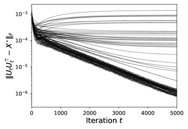
(a) Symmetric matrix sensing

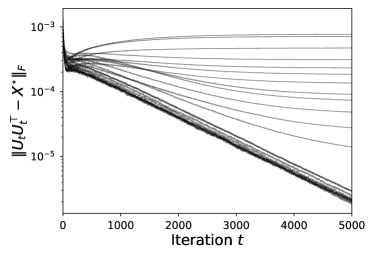
(b) Asymmetric matrix sensing

Figure 2: We apply the sub-gradient method with an exponentially decaying stepsize to noisy instances of symmetric and asymmetric matrix sensing with $\ell_{1}$-loss. When the algorithm is initialized randomly but close enough to the true solution, a significant portion of the trajectories converge to the true solution. This empirical observation supports our conjecture that at least a subset of true solutions emerge as non-active strict saddle points.

1.4 Proof Idea: Parametric Perturbation Sets

Recall that a point ${\mathbf{W}}^{\star}=({W}^{\star}_{1},{W}^{\star}_{2})$ is called a true solution if it satisfies ${W}^{\star}_{1}{W}^{\star}_{2}=X^{\star}$. Accordingly, let $\mathcal{W}$ denote the set of all true solutions $\mathcal{W}=\{(W_{1},W_{2}):W_{1}W_{2}=X^{\star}\}$. The set of true solutions for the symmetric case is similarly defined as $\mathcal{W}=\{W:WW^{\top}=X^{\star}\}$. At a high level, we prove the “inexistence of local minima in $\mathcal{W}$” by proving the following statement: There exists $\gamma_{0}>0$ and $\alpha\geq 1$ such that for every $\gamma\leq\gamma_{0}$

$$\mathbb{P}_{\mathcal{A},\epsilon}\Bigl{(}\max_{\mathbf{W}^{\star}\in\mathcal{W}}\min_{\Delta\mathbf{W}\in\mathcal{B}(\gamma)}\left\{f_{\ell_{1}}(\mathbf{W}^{\star}+\Delta\mathbf{W})-f_{\ell_{1}}(\mathbf{W}^{\star})\right\}\leq-\Omega(\gamma^{\alpha})\Bigr{)}\geq 1-\exp\left(-\operatorname{\textsf{poly}}(d_{1},d_{2},m,r)\right).$$ (1)

In the above inequality, the probability is defined over the possible randomness of the set of measurement matrices $\mathcal{A}=\{A_{1},\dots,A_{m}\}$ and the noise vector $\epsilon$. Moreover, $\operatorname{\textsf{poly}}(d_{1},d_{2},m,r)$ denotes a generic polynomial function of $d_{1},d_{2},m,r$. Finally, $\mathcal{B}(\gamma)$ denotes the Euclidean ball with radius $\gamma$ centered at zero. When the aforementioned inequality is satisfied with $\alpha=1$, it can be asserted with a high probability that none of the true solutions will manifest as critical points. Similarly, if the same inequality holds with $\alpha=2$, with a high probability, all true solutions are either non-critical points or critical but strict saddle points.

The key challenge in proving the above statement lies in characterizing the extremum behavior of the random process $f_{\ell_{1}}(\mathbf{W}^{\star}+\Delta\mathbf{W})-f_{\ell_{1}}(\mathbf{W}^{\star})$ over all $\mathbf{W}^{\star}\in\mathcal{W}$ and $\Delta\mathbf{W}\in\mathcal{B}(\gamma)$. One natural way to prove (1) is by providing an explicit characterization of $\mathbf{W}^{\star}\in\mathcal{W}$ and $\Delta\mathbf{W}\in\mathcal{B}(\gamma)$ that achieve this extremum behavior in terms of the random quantities $\mathcal{A},\epsilon$. Unfortunately, this characterization cannot be expressed explicitly. To circumvent this challenge, we introduce a parametric perturbation set $\mathcal{U}(\gamma,\mathbf{W}^{\star},\mathcal{A},\epsilon)\subset\mathcal{B}({\gamma})$ that exhibits the following key properties:

1. With probability at least $1-\exp\left(-\operatorname{\textsf{poly}}(d_{1},d_{2},m,r)\right)$, the set $\mathcal{U}(\gamma,\mathbf{W}^{\star},\mathcal{A},\epsilon)$ is non-empty for every $\mathbf{W}^{\star}\in\mathcal{W}$ and $\gamma\leq\gamma_{0}$.

2. There exists $\alpha\geq 1$ such that $f_{\ell_{1}}(\mathbf{W}^{\star}+\Delta\mathbf{W})-f_{\ell_{1}}(\mathbf{W}^{\star})\leq-\Omega(\gamma^{\alpha})$ for every $\mathbf{W}^{\star}\in\mathcal{W}$, $\gamma\leq\gamma_{0}$, and $\Delta\mathbf{W}\in\mathcal{U}(\gamma,\mathbf{W}^{\star},\mathcal{A},\epsilon)$.

Indeed, the above two statements together are sufficient to establish the correctness of (1). Our key technical contribution resides in the explicit construction of such parametric perturbation sets that satisfy the aforementioned conditions.

1.5 Related Work

Effect of over-parameterization

For the noiseless symmetric matrix sensing and completion with exactly parameterized rank $k=r$, BM with $\ell_{2}$-loss satisfies the strict saddle property. This property implies that all critical points of the loss function, aside from those corresponding to true solutions, are strict saddle points [BNS16, GLM16]. This result also holds for other variants of low-rank matrix recovery, such as phase retrieval [SQW18], as well as those with more general smooth loss functions [ZLTW18]. In the asymmetric setting, earlier findings have indicated that augmenting BM with a balancing regularizer also maintains the strict saddle property [GJZ17, ZLTW21]. Notably, recent research has demonstrated that the inclusion of the balancing regularization is, in fact, unnecessary for preserving this property [LLZ⁺20]. In cases where the global strict saddle property may not hold globally, it can still be established locally around true solutions, with more lenient conditions [ZZ20, MBLS22]. Recently, these insights have been extended to the over-parameterized regime. Specifically, [Zha22, Zha21] have shown that the BM progressively reduces the occurrence of spurious local minima as the search rank $k$ exceeds the true rank $r$. However, this progress comes at the cost of increasing the sample size proportionally with the search rank $k$. To the best of our knowledge, no existing results establish the strict saddle property of BM with a sample complexity independent of the search rank.

Effect of noise

Another line of work has studied the landscape of BM with $\ell_{1}$-loss, particularly in scenarios where a subset of the measurements are grossly corrupted with noise. Recent results on matrix completion [FS20] and matrix sensing [MF21], focusing on the case where $k=r=1$, have revealed that all critical points either exhibit small norm or closely approximate the true solution, even if up to a constant fraction of the measurements are corrupted with noise [FS20, JL22, MF21]. Generalizing beyond the rank-1 case, only local results are known for the $\ell_{1}$-loss. In particular, [LZMCSV20, CCD⁺21] have shown that, for the symmetric matrix sensing with exactly parameterized rank $k=r$ and $\ell_{1}$-loss, the global minima correspond to the true solutions and there are no spurious critical points locally around the true solutions, even if up to half of the measurements are corrupted with noise. These findings have recently been extended to the over-parameterized regime where $k\geq r$ [DJC⁺21]. However, analogous to the smooth case, the necessary sample size still scales with the search rank. To the best of our knowledge, these results have not been extended to asymmetric matrix sensing, symmetric matrix completion, or asymmetric matrix completion with a general rank configurations.

Convergence guarantees

Achieving global optimality for the true solutions typically necessitates a sample size that scales with the search rank. However, recent studies have revealed a promising contrast in the behavior of local-search algorithms by requiring significantly smaller sample sizes to converge to the true solutions. For instance, in noiseless matrix sensing with an $\ell_{2}$-loss, gradient descent has been shown to converge to the ground truth, provided that the sample size is proportional to the true rank, potentially being substantially smaller than the search rank [SS21, XSCM23, ZFZ22, SSX23]. This result has been extended to matrix sensing with an $\ell_{1}$-loss, where it has been shown that the sub-gradient method, initialized with a small value, can converge to the ground truth when applied to BM with an over-parameterized rank [MF23]. This convergence occurs even in scenarios where the sample size does not scale with the search rank, and an arbitrarily large portion of the measurements is corrupted by noise. These findings strongly suggest the conjecture that the conditions for convergence of local-search algorithms may be considerably less stringent than the requirements for global optimality of the true solutions.

Notations.

For a matrix $M$, its operator, Frobenius, and element-wise $\ell_{q}$ norms are denoted as $\left\lVert M\right\rVert$, $\left\lVert M\right\rVert_{F}$, and $\left\lVert M\right\rVert_{\ell_{q}}$, respectively. For a matrix $M\in\mathbb{R}^{m\times n}$, its singular values are denoted as $\sigma_{1}(M)\geq\sigma_{2}(M)\geq\dots\geq\sigma_{\min\{m,n\}}(M)\geq 0$. The symbol $0_{m\times n}$ refers to $m\times n$ zero matrix. Similarly, we define $I_{m\times n}=[I_{m\times m},0_{m,n-m}]$ if $n>m$, and $I_{m\times n}=[I_{n\times n},0_{n,m-n}]^{\top}$ if $n<m$, where $I_{m\times m}$ and $I_{n\times n}$ are $m\times m$ and $n\times n$ identity matrices, respectively. For two matrices $X$ and $Y$ of the same size, their inner product is shown as $\left\langle X,Y\right\rangle$. The set $\mathcal{B}_{\bar{M}}(\gamma)$ denotes the Euclidean ball with radius $\gamma$ centered at $\bar{M}\in\mathbb{R}^{m\times n}$, i.e., $\mathcal{B}_{\bar{M}}(\gamma):=\{M\in\mathbb{R}^{m\times n}:\left\lVert M-\bar{M}\right\rVert_{F}\leq\gamma\}$; we omit the subscript if the ball is centered at zero. The set $\mathcal{O}_{m,n}$ refers to the set of $m\times n$ orthonormal matrices. More precisely, $\mathcal{O}_{m\times n}:=\{M\in\mathbb{R}^{m\times n}:MM^{\top}=I_{m}\}$ if $m\leq n$, and $\mathcal{O}_{m\times n}:=\{M\in\mathbb{R}^{m\times n}:M^{\top}M=I_{n}\}$ if $n\leq m$. The Kronecker product of two matrices $M$ and $N$ is denoted by $M\otimes N$. For a matrix $M$, $\ker(M)$ and $\dim(\ker(M))$ denote the kernel of $M$ and the dimension of the kernel of $M$, respectively. We use $M[i,j]$ to denote the $(i,j)$-th element of $M$.

Given an integer $n\geq 1$, we define $[n]=\{1,2,\dots,n\}$. Given a subset $\mathcal{I}\in[n]$, we define $\mathcal{I}^{c}=[n]\backslash\mathcal{I}$. The sign function is defined as $\mathrm{sgn}(x)=x/|x|$ if $x\not=0$, and $\mathrm{sgn}(0)\in[-1,1]$. Given two sequences $f(n)$ and $g(n)$, the notation $f(n)\lesssim g(n)$ or $f(n)=O(g(n))$ implies that there exists a universal constant $C>0$ satisfying $f(n)\leq Cg(n)$. We also write $g(n)=\Omega(f(n))$ if $f(n)\lesssim g(n)$. Moreover, the notation $f(n)\asymp g(n)$ implies that $f(n)\lesssim g(n)$ and $g(n)\lesssim f(n)$. Throughout the paper, the symbols $C,c_{1},c_{2},\dots$ refer to universal constants whose precise value may change depending on the context.

2 Main Results

2.1 Problem Formulation

In this work, we study the landscape of BM with $\ell_{1}$-loss for two classes of low-rank matrix recovery, namely matrix sensing and matrix completion. For matrix sensing, the measurement matrices are designed according to the following model.

Assumption 1 (Matrix Sensing Model).

For every $1\leq i\leq m$, the entries of the measurement matrix $A_{i}$ are independently drawn from a standard Gaussian distribution with zero mean and unit variance.

Recall that in BM, the true solution is modeled as $W_{1}W_{2}$, where $W_{1}\in\mathbb{R}^{d_{1}\times k}$ and $W_{2}\in\mathbb{R}^{k\times d_{2}}$ for some search rank $k\geq r$. BM with $\ell_{1}$-loss adapted to matrix sensing is thus formulated as:

$$\min_{W_{1}\in\mathbb{R}^{d_{1}\times k},W_{2}\in\mathbb{R}^{k\times d_{2}}}f^{\mathrm{s}}_{\ell_{1}}(\mathbf{W}):=\frac{1}{m}\sum_{i=1}^{m}\left|y_{i}-\langle A_{i},W_{1}W_{2}\rangle\right|,\quad\text{where}\quad A_{i}[k,l]\stackrel{{\scriptstyle iid}}{{\sim}}\mathcal{N}(0,1),\ \forall i,k,l.$$ (MS-asym)

In symmetric matrix sensing, the true solution $X^{\star}$ is additionally assumed to be positive semidefinite with dimension $d\times d$. In this setting, the true solution can be modeled as $X^{\star}=W^{\star}{W^{\star}}^{\top}$ with $W^{\star}\in\mathbb{R}^{d\times r}$ and BM can be reformulated as:

$$\min_{W\in\mathbb{R}^{d\times k}}f^{\mathrm{s}}_{\ell_{1}}(W):=\frac{1}{m}\sum_{i=1}^{m}\left|y_{i}-\left\langle A_{i},WW^{\top}\right\rangle\right|,\quad\text{where}\quad A_{i}[k,l]\stackrel{{\scriptstyle iid}}{{\sim}}\mathcal{N}(0,1),\forall i,k,l.$$ (MS-sym)

Another important subclass of low-rank matrix recovery is matrix completion, where the linear operator $\mathcal{A}(\cdot)$ is assumed to be element-wise projection.

Assumption 2 (Matrix completion model).

Each index pair $(k,l)$ belongs to a measurement set $\Psi$ with a sampling probability $0\leq s\leq 1$, i.e., $\mathbb{P}((x,y)\in\Psi)=s$ for every $1\leq x\leq d_{1}$ and $1\leq y\leq d_{2}$. Moreover, for every $(x^{\prime},y^{\prime})\in\Psi$, there exists $1\leq i\leq|\Psi|$ such that the measurement matrix $A_{i}$ is defined as $A_{i}[x,y]=1$ if $(x,y)=(x^{\prime},y^{\prime})$ and $A_{i}[x,y]=0$ otherwise.

Based on the above model, we define $Y\in\mathbb{R}^{d_{1}\times d_{2}}$ as $Y[x,y]=y_{i}$ if $A_{i}[x,y]=1$ for some $1\leq i\leq m$ and $(x,y)\in\Psi$, and $Y[x,y]=0$ otherwise. Similarly, we define $E\in\mathbb{R}^{d_{1}\times d_{2}}$ as $E[x,y]=\epsilon_{i}$ if $A_{i}[x,y]=1$ for some $1\leq i\leq m$ and $(x,y)\in\Psi$, and $E[x,y]=0$ otherwise. If the measurements follow matrix completion model, BM can be written as:

$$\min_{W_{1}\in\mathbb{R}^{d_{1}\times k},W_{2}\in\mathbb{R}^{k\times d_{2}}}f^{\mathrm{c}}_{\ell_{1}}(\mathbf{W}):=\frac{1}{m}\sum_{(x,y)\in\Psi}\left|Y[x,y]-(W_{1}W_{2})[x,y]\right|.$$ (MC-asym)

In symmetric matrix completion, the true solution $X^{\star}$ is additionally assumed to be positive semidefinte with dimension $d\times d$. Under this assumption, BM can be written as:

$$\min_{W\in\mathbb{R}^{d\times k}}f^{\mathrm{c}}_{\ell_{1}}(W):=\frac{1}{m}\sum_{(x,y)\in\Psi}\left|Y[x,y]-\left(WW^{\top}\right)[x,y]\right|.$$ (MC-sym)

Finally, we present our noise model.

Assumption 3 (Noise Model).

Each measurement is independently corrupted with noise with a corruption probability $0\leq p\leq 1$. Let the set of noisy measurements be denoted as $\mathcal{S}$. For each entry $i\in\mathcal{S}$, the value of $\epsilon_{i}$ is drawn from a distribution ${P_{o}}$. Moreover, a random variable $\zeta$ under the distribution ${P_{o}}$ satisfies $\mathbb{P}(|\zeta|\geq t_{0})\geq p_{0}$ for some constants $0<t_{0},p_{0}\leq 1$.

Our considered noise model relies on very minimal assumptions and includes all the “typical” noise models, including Gaussian and outlier noise models. Intuitively, it only requires a nonzero mass at a nonzero value. For example, suppose that for every $i\in\mathcal{S}$, $\epsilon_{i}\sim\mathcal{N}(0,\sigma^{2})$. A basic anti-concentration inequality implies that $\mathbb{P}(|\epsilon_{i}|\geq t_{0})=1-\mathbb{P}(|\epsilon_{i}|/\sigma<t_{0}/\sigma)\geq 1-2t_{0}/\sigma$, which satisfies 3 with $(t_{0},p_{0})=\left((4\sigma)^{-1},1/2\right)$. Similarly, a randomized sparse outlier noise is expected to satisfy 3.

2.2 Local Landscape of Matrix Sensing

Symmetric matrix sensing.

Our next two theorems provide necessary and sufficient conditions for the local optimality of the true solutions for symmetric matrix sensing.

Theorem 1 (Sub-optimality of true solutions for symmetric matrix sensing).

Consider MS-sym and measurement matrices satisfying 1. Suppose that the noise satisfies 3. Suppose that $k>r$ and $m\lesssim{pp_{0}d(k-r)}$. With probability at least $1-\exp(-\Omega(d(k-r)))-\exp(-\Omega(pp_{0}m))$, none of the true solutions in $\mathcal{W}$ are local minima of $f^{\mathrm{s}}_{\ell_{1}}(W)$. More precisely, for any $0<\gamma^{2}\lesssim\frac{t_{0}}{\sqrt{d}}$, we have

$$\max_{W^{\star}\in\mathcal{W}}\min_{W\in\mathcal{B}_{W^{\star}}(\gamma)}\left\{f^{\mathrm{s}}_{\ell_{1}}(W)-f^{\mathrm{s}}_{\ell_{1}}(W^{\star})\right\}\lesssim-\gamma^{2}.$$ (2)

According to Theorem 3, to ensure the local optimality of any true solution, the number of measurements must scale with the search rank $k$. In particular, suppose that $2r\leq k$ and the parameters of the noise model are fixed. Then, Theorem 1 shows that, with high probability, none of the true solutions are local minima, so long as $m\lesssim dk$. As shown before, this sample size is significantly larger than what is needed for the sub-gradient method to converge to a true solution.

Our next result complements this result, showing that despite their sub-optimality, all true solutions emerge as critical points so long as $m\gtrsim dr$.

Theorem 2 (Optimality of true solutions for symmetric matrix sensing).

Consider MS-sym with $\ell_{1}$-loss and measurement matrices satisfying 1. Suppose that the noise satisfies 3 with a corruption probablity $0\leq p<1/2$. Finally, suppose that $k\geq r$. The following statements hold:

• Suppose that $m\gtrsim\frac{dr}{(1-2p)^{4}}$. With probability at least $1-\exp(-\Omega(dr))$, all true solutions in $\mathcal{W}$ are critical. More precisely, for any $\gamma\geq 0$, we have

  $$\min_{W^{\star}\in\mathcal{W}}\min_{W\in\mathcal{B}_{W^{\star}}(\gamma)}\left\{f^{\mathrm{s}}_{\ell_{1}}(W)-f^{\mathrm{s}}_{\ell_{1}}(W^{\star})\right\}\gtrsim-\left(\sqrt{\frac{2}{\pi}}+\sqrt{\frac{dk}{m}}\right)\gamma^{2},$$

• Suppose that $m\gtrsim\frac{dk}{(1-2p)^{4}}$. With probability at least $1-\exp(-\Omega(dk))$, all true solutions coincide with the global minima. More precisely, we have

  $$W^{\star}\in\mathcal{W}\quad\iff\quad W^{\star}\in\operatorname*{arg\,min}_{W}f^{\mathrm{s}}_{\ell_{1}}(W).$$

Theorems 1 and 2 together show that the landscape of symmetric matrix sensing with $\ell_{1}$-loss and outlier noise (with $p<1/2$) undergoes two critical transitions: When $m\lesssim dr$, exact recovery is impossible due to the existing information theoretical barriers [CP11]. When $dr\lesssim m\lesssim dk$, all true solutions emerge as critical points and have strictly negative quadratic curvature. We note that this is precisely the regime where the sub-gradient method empirically converges to one of the true solutions, strongly suggesting that at least a subset of the true solutions may be non-active strict saddle points. As soon as $m\gtrsim dk$, all true solutions coincide with the global minima.

Asymmetric matrix sensing.

Next, we consider the asymmetric matrix sensing with $\ell_{1}$-loss, formulated as MS-asym. A key distinction in the asymmetric setting lies in the existence of rank-imbalanced solutions, i.e., true solutions $(W^{\star}_{1},W^{\star}_{2})\in\mathcal{W}$ with $2r<\mathrm{rank}(W^{\star}_{1})+\mathrm{rank}(W^{\star}_{2})\leq 2k$. To illustrate this, consider the SVD of the true solution $X^{\star}=U^{\star}\Sigma^{\star}{V^{\star\top}}$ and suppose $k>r$. Indeed, the point $\mathbf{W}^{\star}=(W^{\star}_{1},W^{\star}_{2})$ with $W^{\star}_{1}=\begin{bmatrix}U^{\star}\Sigma^{\star}&0_{d_{1}\times(k-r)}\end{bmatrix},W^{\star}_{2}=\begin{bmatrix}{V^{\star}}&Z\end{bmatrix}^{\top}$ is a true solution for any arbitrary $Z\in\mathbb{R}^{d_{2}\times(k-r)}$. Moreover, $\mathrm{rank}(W^{\star}_{1})+\mathrm{rank}(W^{\star}_{2})=r+k>2r$, provided that $Z$ is chosen such that $W^{\star}_{2}$ is full row-rank. In contrast, any true solution $W^{\star}$ for the symmetric matrix recovery inevitably must satisfy $\mathrm{rank}(W^{\star})=r$, and hence, is rank-balanced. As we will demonstrate later, the existence of rank-imbalanced solutions drastically changes the local landscape of asymmetric matrix recovery.

To formalize our ideas, we first introduce some notations. For any matrix $E$ and $\tau\geq 0$, let $\mathrm{rank}(E,\tau)$ be the number of singular values of $E$ that are strictly greater than $\tau$. Evidently, we have $\mathrm{rank}(E,0)=\mathrm{rank}(E)$. Let the SVD of $E$ be $V_{1}\Sigma V_{2}$. Define $E(\tau)=V_{1}\Sigma_{\tau}V_{2}$, where $\Sigma_{\tau}$ corresponds to $\Sigma$ after thresholding out the singular values that are upper bounded by $\tau$. Evidently, $E(\tau)$ is the minimizer of $\left\lVert M-E\right\rVert_{F}$ among all the matrices $M$ with a rank no greater than $\mathrm{rank}(E,\tau)$. Therefore, we have $\mathrm{rank}(E(\tau))=\mathrm{rank}(E,\tau)$. Finally, we define

$$\mathcal{W}(\tau,s)=\left\{(W_{1},W_{2})\in\mathcal{W}:\mathrm{rank}(W_{1},\tau)+\mathrm{rank}(W_{2},\tau)\leq s\right\}.$$

To analyze the landscape of the asymmetric matrix sensing, we divide the set of true solutions into two subsets: $\mathcal{W}=\mathcal{W}(\tau,2k/3)\cup\left(\mathcal{W}\backslash\mathcal{W}(\tau,2k/3)\right)$ for some $\tau>0$. We call the set $\mathcal{W}\backslash\mathcal{W}(\tau,2k/3)$ the set of rank-imbalanced solutions. To see this, suppose that $k>3r$. Then, for any $\mathbf{W}^{\star}=(W^{\star}_{1},W^{\star}_{2})\in\mathcal{W}\backslash\mathcal{W}(\tau,2k/3)$, we have $\mathrm{rank}(W^{\star}_{1})+\mathrm{rank}(W^{\star}_{2})>2r$. In other words, for any true solution in $\mathcal{W}\backslash\mathcal{W}(\tau,2k/3)$, at least one of the factors has a rank that is higher than the true rank.

Theorem 3 (Sub-optimality of true solutions for asymmetric matrix sensing).

Consider MS-asym with $\ell_{1}$-loss and measurement matrices satisfying 1. Suppose that the noise satisfies 3 and $k\geq r$. With probability at least $1-\exp(-\Omega(p_{0}pm))$, the following statements hold:

• Suppose that $m\lesssim\max\{d_{1},d_{2}\}k$. Then, none of the true solutions in $\mathcal{W}(0,2k/3)$ are local minima. More precisely, for any $0<\gamma\lesssim\sqrt{\frac{mpp_{0}}{\max\{d_{1},d_{2}\}k}}t_{0}$, we have

  $$\max_{\mathbf{W}^{\star}\in\mathcal{W}\backslash\mathcal{W}(0,k/3)}\min_{\mathbf{W}\in\mathcal{B}_{\mathbf{W}^{\star}}(\gamma)}\left\{f^{\mathrm{s}}_{\ell_{1}}(\mathbf{W})-f^{\mathrm{s}}_{\ell_{1}}(\mathbf{W}^{\star})\right\}\lesssim-\sqrt{\frac{\max\{d_{1},d_{2}\}pp_{0}}{m}}\gamma^{2}.$$

• Suppose that $m\lesssim\max\{d_{1},d_{2}\}k$ and there exist constants $0<c_{1}\leq c_{2}<1$ such that $c_{1}\leq\frac{\min\{d_{1},d_{2}\}}{\max\{d_{1},d_{2}\}}\leq c_{2}$. Then, for any $\tau>0$, none of the true solutions in $\mathcal{W}\backslash\mathcal{W}(\tau,2k/3)$ are critical points. More precisely, for any $0<\gamma\lesssim\sqrt{\frac{mpp_{0}}{\min\{d_{1},d_{2}\}k}}\cdot\frac{t_{0}}{\tau}$, we have

  $$\max_{\mathbf{W}^{\star}\in\mathcal{W}\backslash\mathcal{W}(\tau,k/3)}\min_{\mathbf{W}\in\mathcal{B}_{\mathbf{W}^{\star}}(\gamma)}\left\{f^{\mathrm{s}}_{\ell_{1}}(\mathbf{W})-f^{\mathrm{s}}_{\ell_{1}}(\mathbf{W}^{\star})\right\}\lesssim-\sqrt{\frac{\min\{d_{1},d_{2}\}kpp_{0}}{m}}\cdot\tau\gamma.$$

• Suppose that $m\lesssim\max\{d_{1},d_{2}\}k$ and there exist constants $0<c_{1}\leq c_{2}<1$ such that $c_{1}\leq\frac{\min\{d_{1},d_{2}\}}{\max\{d_{1},d_{2}\}}\leq c_{2}$. Then, none of the true solutions are local minima. More precisely, for any $0<\gamma\lesssim\sqrt{\frac{mpp_{0}}{\max\{d_{1},d_{2}\}k}}{t_{0}}$, we have

  $$\max_{\mathbf{W}^{\star}\in\mathcal{W}}\min_{\mathbf{W}\in\mathcal{B}_{\mathbf{W}^{\star}}(\gamma)}\left\{f^{\mathrm{s}}_{\ell_{1}}(\mathbf{W})-f^{\mathrm{s}}_{\ell_{1}}(\mathbf{W}^{\star})\right\}\lesssim-{\frac{pp_{0}\sqrt{k}}{m}}\cdot\gamma^{2}.$$

Theorem 3 shows that, similar to the symmetric case, in order to ensure the local optimality of any true solution for the asymmetric matrix sensing, the number of measurements must scale with the search rank $k$. Moreover, Theorem 3 provides another negative result: no matter how small the corruption probability $p>0$ is, none of the rank-imbalanced solutions are critical points of BM, provided that $m\lesssim\max\{d_{1},d_{2}\}k$ and $c_{1}\leq\frac{\min\{d_{1},d_{2}\}}{\max\{d_{1},d_{2}\}}\leq c_{2}$. As a result, the rank-imbalanced solutions remain beyond the reach of any first-order optimization method designed to converge to a critical point. Finally, we note that the requirement $c_{1}\leq\frac{\min\{d_{1},d_{2}\}}{\max\{d_{1},d_{2}\}}\leq c_{2}$ may be a result of our current proof technique and could potentially be relaxed with a more refined analysis.

The second statement of Theorem 3 is in contrast to the landscape of symmetric matrix sensing, where it is shown that all true solutions become critical if the sample size exceeds $dr$. Nonetheless, our next theorem shows that, unlike the rank-imbalanced solutions, the rank-balanced solutions do in fact emerge as critical points, provided that $m\gtrsim\max\{d_{1},d_{2}\}r$.

Theorem 4 (Optimality of true solutions for asymmetric matrix sensing).

Consider MS-asym with $\ell_{1}$-loss and measurement matrices satisfying 1. Suppose that the noise satisfies 3 with a corruption probability $0\leq p<1/2$. Finally, suppose that $k\geq r$. The following statements hold:

• Suppose that $m\gtrsim\frac{\max\{d_{1},d_{2}\}r}{(1-2p)^{4}}$. With probability at least $1-\exp(-\Omega(\max\{d_{1},d_{2}\}r))$, all true solutions in $\mathcal{W}(0,2r)$ are critical. More precisely, for any $\gamma\geq 0$, we have

  $$\min_{\mathbf{W}^{\star}\in\mathcal{W}(0,r)}\min_{\mathbf{W}\in\mathcal{B}_{\mathbf{W}^{\star}}(\gamma)}\left\{f^{\mathrm{s}}_{\ell_{1}}(\mathbf{W})-f^{\mathrm{s}}_{\ell_{1}}(\mathbf{W}^{\star})\right\}\gtrsim-\left(\sqrt{\frac{2}{\pi}}+\sqrt{\frac{\max\{d_{1},d_{2}\}k}{m}}\right)\gamma^{2}.$$

• Suppose that $m\gtrsim\frac{\max\{d_{1},d_{2}\}k}{(1-2p)^{4}}$. With probability at least $1-\exp(-\Omega(\max\{d_{1},d_{2}\}k))$, all true solutions coincide with the global minima. More precisely, we have

  $$\mathbf{W}^{\star}\in\mathcal{W}\quad\iff\quad\mathbf{W}^{\star}\in\operatorname*{arg\,min}_{\mathbf{W}}f^{\mathrm{s}}_{\ell_{1}}(\mathbf{W}).$$

Combining the findings of Theorem 3 with the results obtained above, we can conclude that rank-balanced solutions emerge as strict saddle points of MS-asym with an $\ell_{1}$-loss. This result, combined with our empirical experiments, reinforces the conjecture that a subset of the true solutions are non-active strict saddle points.

2.3 Local Landscape of Matrix Completion

Symmetric matrix completion.

Next, we study the local landscape of symmetric matrix completion around its true solutions.

Theorem 5 (Sub-optimality of true solutions for symmetric matrix completion).

Consider MC-sym with $\ell_{1}$-loss and measurement matrices satisfying 2. Suppose that $k>r$ and there exists $(l,l)\in\Psi$ such that $E[l,l]\geq t_{0}$. Then, with probability at least $1-\exp(-\Omega(sd_{1}d_{2}))$, none of the true solutions in $\mathcal{W}$ are local minima of $f^{\mathrm{c}}_{\ell_{1}}(W)$. More precisely, for any $W^{\star}\in\mathcal{W}$ and $0<\gamma\lesssim\sqrt{t_{0}}$, we have

$$\max_{W^{\star}\in\mathcal{W}}\min_{W\in\mathcal{B}_{W^{\star}}(\gamma)}\left\{f^{\mathrm{c}}_{\ell_{1}}(W)-f^{\mathrm{c}}_{\ell_{1}}(W^{\star})\right\}\lesssim-\frac{\gamma^{2}}{sd^{2}}.$$

Unlike our previous results, the necessary condition for the local optimality of the true solutions does not rely on the randomness of the noise: none of the true solutions are local or global so long as $k>r$ and at least one of the diagonal entries of $X^{\star}$ is observed with a positive noise. The latter condition is indeed very mild and holds with a high probability, provided that the noise takes a positive value with a nonzero probability. For instance, suppose that $\mathbb{P}(\epsilon_{i}\geq t_{0})\geq p_{+}>0$. Then, the probability of $E[l,l]\geq t_{0}$ for some $(l,l)\in\Psi$ is at least $1-(1-spp_{+})^{d}$. Moreover, this result holds even in a near-ideal scenario, where the sampling probability is equal to 1 (i.e., the entire matrix $X^{\star}$ is observed).

Asymmetric matrix completion.

Our next theorem extends the above result to the asymmetric matrix completion under additional conditions on $X^{\star}$. To achieve this goal, we first introduce the notion of coherence for a matrix.

Definition 1.

Consider a rank-$r$ matrix $M\in\mathbb{R}^{d_{1}\times d_{2}}$ and its SVD $M=U\Sigma{V}^{\top}$, where $U\in\mathbb{R}^{d_{1}\times r}$ and $V\in\mathbb{R}^{d_{2}\times r}$ are the left and right singular vectors corresponding to its nonzero singular values. The matrix $M$ is called coherent if

$$\max\left\{\max_{1\leq i\leq r}\left\lVert Ue_{i}\right\rVert_{\infty},\max_{1\leq i\leq r}\left\lVert Ve_{i}\right\rVert_{\infty}\right\}=1.$$

Based on the above definition, a matrix is coherent if at least one of its left or right singular vectors is aligned with a standard unit vector. It is easy to see that if the ground truth $X^{\star}$ is coherent, the necessary sampling probability can grow to a value of 1. Our next theorem shows that, in the presence of noise, even a sampling probability of $s=1$ is insufficient to ensure that a coherent ground truth emerges as a critical point.

Theorem 6 (Sub-optimality of true solutions for asymmetric matrix completion).

Consider MC-asym with $\ell_{1}$-loss and measurement matrices satisfying 2. Suppose that the noise satisfies 3. With probability at least $1-\exp(-\Omega(spp_{0}\max\{d_{1},d_{2}\}(k-r)))$, the following statements hold:

• Suppose that $k>r$. There exists at least one true solution $\mathbf{W}^{\star}\in\mathcal{W}$ that is not a critical point of $f^{\mathrm{c}}_{\ell_{1}}(\mathbf{W})$. More precisely, for any $0<\gamma\lesssim t_{0}$, we have

  $$\min_{\mathbf{W}\in\mathcal{B}_{\mathbf{W}^{\star}}(\gamma)}\left\{f^{\mathrm{c}}_{\ell_{1}}(\mathbf{W})-f^{\mathrm{c}}_{\ell_{1}}(\mathbf{W}^{\star})\right\}\lesssim-\sqrt{\frac{k-r}{d_{2}}}\cdot\sqrt{\frac{pp_{0}}{sd_{1}d_{2}}}\cdot\gamma.$$

• Suppose that $k>2r$. None of the true solutions in $\mathcal{W}(0,k-1)$ are local minima of $f^{\mathrm{c}}_{\ell_{1}}(\mathbf{W})$. More precisely, for any $0<\gamma\lesssim\sqrt{t_{0}}$, we have

  $$\max_{\mathbf{W}^{\star}\in\mathcal{W}(0,k-1)}\min_{\mathbf{W}\in\mathcal{B}_{\mathbf{W}^{\star}}(\gamma)}\left\{f^{\mathrm{c}}_{\ell_{1}}(\mathbf{W})-f^{\mathrm{c}}_{\ell_{1}}(\mathbf{W}^{\star})\right\}\lesssim-\frac{\gamma^{2}}{sd_{1}d_{2}}.$$

• Suppose that $k\geq r$ and $X^{\star}$ is coherent. None of the true solutions with a bounded norm are critical points of $f^{\mathrm{c}}_{\ell_{1}}(\mathbf{W})$. More precisely, for any radius $\Gamma<\infty$, let $\mathcal{B}_{\mathrm{op}}(\Gamma)=\{(W_{1},W_{2}):\max\{\left\lVert W_{1}\right\rVert,\left\lVert W_{2}\right\rVert\}\leq\Gamma\}$. For any $0<\gamma\lesssim t_{0}$, we have

  $$\max_{\mathbf{W}^{\star}\in\mathcal{W}\cap\mathcal{B}_{\mathrm{op}}(\Gamma)}\min_{\mathbf{W}\in\mathcal{B}_{\mathbf{W}^{\star}}(\gamma)}\left\{f^{\mathrm{c}}_{\ell_{1}}(\mathbf{W})-f^{\mathrm{c}}_{\ell_{1}}(\mathbf{W}^{\star})\right\}$$

  $$\lesssim-\sqrt{\frac{pp_{0}}{sd_{1}d_{2}^{2}}}\cdot\frac{\sigma_{r}(X^{\star})\gamma}{\Gamma}.$$

Theorem 6 shows that, similar to the asymmetric matrix sensing, non-critical true solutions are ubiquitous in the asymmetric matrix completion. In particular, the first statement showcases that, even if the search rank is only slightly over-parameterized (e.g., $k=r+1$), there exists at least one true solution that is non-critical. This result holds with a high probability, even with the sampling probability of $s=1$ provided that $pp_{0}>0$. The second statement, on the other hand, shows that when $k>2r$, none of the true solutions with $\mathrm{rank}(W^{\star}_{1})+\mathrm{rank}(W^{\star}_{2})<k$—including the rank-balanced solutions that satisfy $\mathrm{rank}(W^{\star}_{1})=\mathrm{rank}(W^{\star}_{1})=r$—are local minima of the loss function. We note that this result does not refute the possibility of existing highly rank-imbalanced solutions—in particular, those with $\mathrm{rank}(W^{\star}_{1})+\mathrm{rank}(W^{\star}_{2})\geq k$—as local minima. Although our result does not refute this possibility, we conjecture that highly rank-imbalanced solutions are unlikely to emerge as local minima. We leave a rigorous proof of this conjecture for future work. Finally, the last statement shows that the asymmetric matrix completion with coherent ground truth has the most undesirable landscape; even in the exactly-parameterized regime with $k=r$ and with sampling probability of $s=1$, none of the true solutions are critical points, so long as $pp_{0}>0$. This complements the existing results for the asymmetric matrix completion, which show that the ground truth can be recovered exactly, provided that it is incoherent, i.e., it does not have a significant alignment with the standard basis vectors [CLMW11, CSPW11, Che15].

The rest of the paper is organized as follows. in Section 3, we introduce and elaborate on a collection of tools from variational analysis and random processes that will serve as foundational elements in our subsequent analysis. In Section 4, we prove our results for the symmetric matrix sensing and symmetric matrix completion (Theorems 1 and 5). In Sections 5, we extend our analysis to the asymmetric settings (Theorems 3 and 6). Finally, in Section 6, we present the proofs of our provided lower bounds (Theorems 2 and 4).

3 Preliminaries

In Subsection 3.1, we review basic definitions and results from variational analysis that will be instrumental in developing our results. Then, in Subsections 3.2 to 3.5, we lay the groundwork for certain concentration results for different classes of random variables and random processes that will be used throughout our proofs.

3.1 Basic Properties from Variational Analysis

For a function $f:\mathbb{R}^{n}\to\mathbb{R}$, a point $\bar{x}$ is called a global minimum if it corresponds to its global minimizer. Moreover, a point $\bar{x}$ is called a local minimum if it corresponds to the minimum of $f(x)$ within an open ball centered at $\bar{x}$. The directional derivative of $f$ at point $x$ in the feasible direction $d$ is defined as

$$f^{\prime}(x,d)=\lim_{t\to 0^{+}}\frac{f(x+td)-f(x)}{t},$$

provided that the limit exists. If $f^{\prime}(x,d)<0$, then $d$ is called a descent direction. For a locally Lipschitz function $f$, the Clarke generalized directional derivative at the point $x$ in the feasible direction $d$ is defined as

$$f^{\circ}(x,{d}):=\underset{\begin{subarray}{c}y\rightarrow x\\ t\to 0^{+}\end{subarray}}{\lim\sup}\frac{f(y+t{d})-f(y)}{t}$$

provided that the limit exists. It is a well-known fact that $f^{\prime}(x,d)\leq f^{\circ}(x,d)$ for every direction $d$ if both $f^{\prime}(x,d)$ and $f^{\circ}(x,d)$ exist [Cla75, Proposition 1.4]. A function $f$ is called subdifferentially regular if $f^{\prime}(x,d)=f^{\circ}(x,d)$ for every direction $d$ [Cla90, Definition 2.3.4]. The Clarke subdifferential of $f$ at ${x}$ is defined as the following set (see [Cla75, Definition 1.1 and Proposition 1.4]):

$$\partial f({x}):=\{{\psi}|f^{\circ}(x,{d})\geq\langle{\psi},{d}\rangle,\forall{d}\in\mathbb{R}^{n}\}.$$ (3)

A point $\bar{x}$ is called critical if $0\in\partial f(\bar{x})$, or equivalently, $f^{\circ}(\bar{x},{d})\geq 0$ for every feasible direction $d$. The following properties of the critical points are adapted from [LSM20] and will be used in our subsequent arguments.

Lemma 1.

For a real-valued locally Lipschitz function $f:\mathbb{R}^{n}\to\mathbb{R}$, we have:

1. Every local minimum of $f$ is critical.

2. Given a point $x$, suppose that $f^{\prime}(x,d)\geq 0$ for every feasible $d\in\mathbb{R}^{n}$. Then, $x$ is a critical point of $f$.

3. Suppose that $f=\max_{1\leq i\leq m}g_{i}$ for some smooth functions $g_{1},\dots,g_{m}$. Given some point $x$, suppose that $f^{\prime}(x,d)<0$ for some feasible direction $d\in\mathbb{R}^{n}$. Then, $x$ is not a critical point of $f$.

Proof.

The first property is a direct consequence of [Cla90, Proposition 2.3.2]. The second property follows from the basic inequality $f^{\prime}(x,d)\leq f^{\circ}(x,d)$ [Cla75, Proposition 1.4] and the definition of the critical points. Finally, due to [RW09, Example 7.28], $f$ is differentiably regular, and hence, $f^{\circ}(x,d)=f^{\prime}(x,d)$ for every feasible direction $d$. This implies that $x$ is not critical due to the existence of a direction $d$ for which $f^{\circ}(x,d)=f^{\prime}(x,d)<0$. ∎

Utilizing the above properties, the following crucial lemma provides a sufficient condition for the non-criticality of a point $\bar{\mathbf{W}}$ for the $\ell_{1}$-loss $f_{\ell_{1}}(\mathbf{W})$.

Lemma 2.

Given a point $\bar{\mathbf{W}}$, suppose that there exists a direction $\Delta\mathbf{W}$ such that $f^{\prime}_{\ell_{1}}(\bar{\mathbf{W}},\Delta\mathbf{W})<0$. Then, $\bar{\mathbf{W}}$ is not a critical point of $f_{\ell_{1}}(\mathbf{W})$.

Proof.

We first define $\mathcal{M}$ as the class of binary functions $\sigma:\{1,\dots,m\}\to\{-1,+1\}$. It is easy to see that $f_{\ell_{1}}(\mathbf{W})=\max_{\sigma\in\mathcal{M}}g_{\sigma}(\mathbf{W})$, where $g_{\sigma}(\mathbf{W})=\sum_{i\in m}\sigma(i)\left(y_{i}-\left\langle A_{i},W_{1}W_{2}\right\rangle\right)$. Note that $g_{\sigma}(\mathbf{W})$ is smooth for any choice of $\sigma\in\mathcal{M}$. Therefore, the third property of Lemma 1 can be invoked to complete the proof. ∎

3.2 Orlicz Random Variables and Processes

First, we define the notion of Orlicz norm (see [Wai19, Section 5.6] and [LT91, Section 11.1] for more details).

Definition 2 (Orlicz function and Orlicz norm).

A function $\psi:\mathbb{R}_{+}\to\mathbb{R}_{+}$ is called an Orlicz function if $\psi$ is convex, increasing, and satisfies

$$\psi(0)=0,\quad\psi(x)\to\infty\text{ as }x\to\infty.$$

For a given Orlicz function $\psi$, the Orlicz norm of a random variable $X$ is defined as

$$\left\lVert X\right\rVert_{\psi}:=\inf\{t>0:\mathbb{E}[\psi(|X|/t)]\leq 1\}.$$

We will use Orlicz functions and norms to study the concentration of both sub-Gaussian and sub-exponential random variables, which are defined as follows.

Definition 3 (Sub-Gaussian and sub-exponential random variables).

Define the Orlicz function $\psi_{p}(x)=\exp\{x^{p}\}-1$. A random variable $X$ is called sub-Gaussian if $\left\lVert X\right\rVert_{\psi_{2}}<\infty$. Moreover, a random variable $X$ is called sub-exponential if $\left\lVert X\right\rVert_{\psi_{1}}<\infty$. Accordingly, the quantities $\left\lVert X\right\rVert_{\psi_{2}}$ and $\left\lVert X\right\rVert_{\psi_{1}}$ refer to the sub-Gaussian norm and sub-exponential norm of $X$, respectively.

Lemmas 3-6 establish basic properties of sub-Gaussian and sub-exponential random variables.

Lemma 3 (Tail bounds for sub-Gaussian and sub-exponential random variables [Wai19, Section 5.6]).

For a random variable $X$ with finite Orlicz norm $\left\lVert X\right\rVert_{\psi_{p}}<\infty$ where $\psi_{p}(x)=\exp\{x^{p}\}-1$ and $p\geq 1$, we have

$$\mathbb{P}\left(|X|\geq\delta\right)\leq 2\exp\left(-\frac{\delta^{p}}{\left\lVert X\right\rVert_{\psi_{p}}^{p}}\right).$$

Lemma 4 (Sum of independent random variables [Ver18, Theorems 2.6.2 and 2.8.1]).

Let $X_{1},\cdots,X_{n}$ be zero-mean independent random variables.

• If each $X_{i}$ is sub-Gaussian with sub-Gaussian norm $\left\lVert X_{i}\right\rVert_{\psi_{2}}$, we have

  $$\mathbb{P}\left(\left|\frac{1}{n}\sum_{i=1}^{n}X_{i}\right|\geq\delta\right)\leq 2\exp\left(-\frac{n^{2}\delta^{2}}{\sum_{i=1}^{n}\left\lVert X_{i}\right\rVert_{\psi_{2}}^{2}}\right).$$

• If each $X_{i}$ is sub-exponential with sub-exponential norm $\left\lVert X_{i}\right\rVert_{\psi_{1}}$, we have

  $$\mathbb{P}\left(\left|\frac{1}{n}\sum_{i=1}^{n}X_{i}\right|\geq\delta\right)\leq 2\exp\left(-n\min\left\{\frac{\delta^{2}}{\max_{i}\left\lVert X_{i}\right\rVert_{\psi_{1}}^{2}},\frac{\delta}{\max_{i}\left\lVert X_{i}\right\rVert_{\psi_{1}}}\right\}\right).$$

Lemma 5 (Lemma 2.6.8 in [Ver18]).

Suppose that $X$ is sub-Gaussian. We have $\left\lVert X-\mathbb{E}[X]\right\rVert_{\psi_{2}}\leq C\left\lVert X\right\rVert_{\psi_{2}}$ for some constant $C>0$.

Lemma 6 (Lemma 2.7.7 in [Ver18]).

Let $X,Y$ be sub-Gaussian random variables. Then $XY$ is sub-exponential with its sub-exponential norm satisfying $\left\lVert XY\right\rVert_{\psi_{1}}\leq\left\lVert X\right\rVert_{\psi_{2}}\left\lVert Y\right\rVert_{\psi_{2}}$.

Next, we introduce the notion of Orlicz process.

Definition 4 (Orlicz process, Definition 5.35 in [Wai19]).

A set of zero-mean random variables $\{X_{t},t\in\mathcal{T}\}$ (also known as a stochastic process) is an Orlicz process with Orlicz norm $\psi_{p}$ (also known as $\psi_{p}$-process) with respect to a metric $d$ if

$$\left\lVert X_{t}-X_{t^{\prime}}\right\rVert_{\psi_{p}}\leq d(t,t^{\prime})\quad\text{for all }t,t^{\prime}\in\mathcal{T}.$$

According to the above definition, the size of the set $\mathcal{T}$ may be infinite. To control the behavior of a $\psi_{p}$-process, we first need the notions of $\epsilon$-covering and covering number.

Definition 5 (Covering and covering number).

A set $\mathcal{N}_{\epsilon}(\mathcal{T})$ is called an $\epsilon$-covering on $(\mathcal{T},d)$ if for every $t\in\mathcal{T}$, there exists $\pi(t)\in\mathcal{N}_{\epsilon}(\mathcal{T})$ such that $d(t,\pi(t))\leq\epsilon$. The covering number $\mathcal{N}(\mathcal{T},d,\epsilon)$ is defined as the smallest cardinality of an $\epsilon$-covering for $(\mathcal{T},d)$:

$$\mathcal{N}(\mathcal{T},d,\epsilon):=\inf\{|\mathcal{N}_{\epsilon}(\mathcal{T})|:\mathcal{N}_{\epsilon}(\mathcal{T})\text{ is an }\epsilon\text{-covering for }(\mathcal{T},d)\}.$$

Theorem 7 (Concentration of Orlicz process, Theorem 5.36 in [Wai19]).

Let $\{X_{t},t\in\mathcal{T}\}$ be a $\psi_{p}$-process with respect to the metric $d$. Then, there is a universal constant $C>0$ such that

$$\mathbb{P}\left(\sup_{t\in\mathcal{T}}X_{t}\geq C\mathcal{J}_{p}(0,D)+\delta\right)\leq\exp({-{\delta^{p}}/{D^{p}}}).$$

Here $D=\sup_{t,t^{\prime}\in\mathcal{T}}d(t,t^{\prime})$ is the diameter of the set $\mathcal{T}$ and $\mathcal{J}_{p}(\delta,D)=\int_{\delta}^{D}\log^{1/p}\left(1+\mathcal{N}(\mathcal{T},d,\epsilon)\right)d\epsilon$ is called the generalized Dudley entropy integral.

By providing tractable upper bounds on $D$ and $\mathcal{J}_{p}(\delta,D)$, one can control the supremum of a $\psi_{p}$-process. In our next section, we provide specific sub-classes of $\psi_{p}$-process for which these quantities can be controlled efficiently.

3.3 Concentration Bounds for Gaussian Processes over Grassmannian Manifold

In our subsequent analysis, Gaussian processes defined over the Grassmannian manifold, which are a specific category of Orlicz processes, will play a pivotal role. To set the stage, we start with the definition of a Gaussian process.

Definition 6 (Gaussian process).

A random process $\{X_{t}\}_{t\in\mathcal{T}}$ is called a Gaussian process if, for any finite subset $\mathcal{T}_{0}\subset\mathcal{T}$, the random vector $\{X_{t}\}_{t\in\mathcal{T}_{0}}$ has a normal distribution.

Our next lemma characterizes the expectation of the supremum of a Gaussian process in terms of its covering number.

Theorem 8 (Sudakov’s minoration inequality, Theorem 5.30 in [Wai19]).

Let $\{X_{t}\}_{t\in\mathcal{T}}$ be a zero-mean Gaussian process. Then, for any $\epsilon\geq 0$, we have

$$\mathbb{E}\left[\sup_{t\in\mathcal{T}}X_{t}\right]\geq\frac{\epsilon}{2}\sqrt{\log\mathcal{N}(\mathcal{T},d,\epsilon)}.$$

Here, the metric $d$ is defined as $d(t_{1},t_{2})=\left(\mathbb{E}\left[(X_{t_{1}}-X_{t_{2}})^{2}\right]\right)^{1/2}$ for any $t_{1},t_{2}\in\mathcal{T}$.

Lemma 7 (Concentration of Gaussian Process, Lemma 6.12 in [VH14]).

Let $\{X_{t}\}_{t\in\mathcal{T}}$ be a Gaussian process. Then $\sup_{t\in\mathcal{T}}X_{t}$ is sub-Gaussian with sub-Gaussian norm $\sup_{t\in\mathcal{T}}\left\lVert X_{t}\right\rVert_{\psi_{2}}$.

Next, we provide the definition of Grassmanian manifold.

$$\mathcal{G}(n,p)=\{P\in\mathbb{R}^{n\times n}:P^{\top}=P,P^{2}=P,\mathrm{rank}(P)=p\}.$$ (4)

Our next lemma characterizes the covering number of the Grassmannian manifold $\mathcal{G}(n,p)$.

Lemma 8 (Covering number for Grassmannian manifold, Proposition 8 in [Sza82]).

For a Grassmannian manifold $\mathcal{G}(n,p)$, define the metric $d(P_{1},P_{2})=\left\lVert P_{1}-P_{2}\right\rVert_{F}$ for any $P_{1},P_{2}\in\mathcal{G}(n,p)$. Then, for any $0<\epsilon<\sqrt{2\min\{p,n-p\}}$, we have

$$\left(\frac{c_{1}\sqrt{p}}{\epsilon}\right)^{p(n-p)}\leq\mathcal{N}(\mathcal{G}(n,p),d,\epsilon)\leq\left(\frac{c_{2}\sqrt{p}}{\epsilon}\right)^{p(n-p)},$$

for some constants $c_{1},c_{2}>0$.

Lemma 9 (Lower bound of Gaussian process over Grassmannian manifold).

Consider the Gaussian process $\sup_{X\in\mathcal{G}(n,p)}\left\langle A,X\right\rangle$, where $A$ is a standard Gaussian matrix and $p\leq n/2$. Then, with probability at least $1-\exp({-\Omega(np)})$, we have

$$\sup_{X\in\mathcal{G}(n,p)}\left\langle A,X\right\rangle\geq\frac{c_{3}}{2}\sqrt{np^{2}},$$

for $c_{3}=\sqrt{\log(c_{1})/8}$, where $c_{1}$ is the constant appeared in Lemma 8.

Proof.

We first use Sudakov’s Minoration Inequality (Theorem 8) to characterize the expectation of the supremum:

$$\mathbb{E}\left[\sup_{X\in\mathcal{G}(n,p)}\left\langle A,X\right\rangle\right] \geq\sup_{0<\epsilon}\frac{\epsilon}{2}\sqrt{\log\mathcal{N}\left(\mathcal{G}(n,p),\left\lVert\cdot\right\rVert_{F},\epsilon\right)}$$

$$\stackrel{{\scriptstyle(a)}}{{\geq}}\sup_{0<\epsilon\leq\sqrt{2p}}\frac{\epsilon}{2}\sqrt{p(n-p)\log\left(\frac{c_{1}\sqrt{p}}{\epsilon}\right)}$$

$$\stackrel{{\scriptstyle\text{set }\epsilon=\sqrt{p}}}{{\geq}}\frac{1}{2}\sqrt{(n-p)p^{2}\log(c_{1})}$$

$$\geq c_{3}\sqrt{np^{2}}.$$

In (a), we invoked the lower bound on the covering number $\mathcal{N}\left(\mathcal{G}(n,p),\left\lVert\cdot\right\rVert_{F},\epsilon\right)$ from Lemma 8. Next, we apply Lemma 7 to control the deviation of the supremum from its expectation. To this goal, we first note that for any $X\in\mathcal{G}(n,p)$, we have $\left\lVert\left\langle A,X\right\rangle\right\rVert_{\psi_{2}}\leq\left\lVert X\right\rVert_{F}=\sqrt{p}$. According to Lemma 7, $\sup_{X\in\mathcal{G}(n,p)}\left\langle A,X\right\rangle$ is sub-Gaussian with norm $\sqrt{p}$. Due to Definition 3, we have

$$\mathbb{P}\left(\sup_{X\in\mathcal{G}(n,p)}\left\langle A,X\right\rangle-c_{3}\sqrt{np^{2}}\leq-\delta\right) \leq\mathbb{P}\left(\sup_{X\in\mathcal{G}(n,p)}\left\langle A,X\right\rangle-\mathbb{E}\left[\sup_{X\in\mathcal{G}(n,p)}\left\langle A,X\right\rangle\right]\leq-\delta\right)$$

$$\leq\exp\left\{-\frac{\delta^{2}}{\left\lVert\sup_{X\in\mathcal{G}(n,p)}\left\langle A,X\right\rangle\right\rVert_{\psi_{2}^{2}}}\right\}$$

$$\leq\exp\left\{-\delta^{2}/p\right\}.$$

Upon setting $\delta=\frac{c_{3}}{2}\sqrt{np^{2}}$, we know that with probability at least $1-\exp({-\Omega(np)})$

$$\sup_{X\in\mathcal{G}(n,p)}\left\langle A,X\right\rangle\geq\frac{c_{3}}{2}\sqrt{np^{2}},$$

which completes the proof. ∎

Our next lemma provides another useful bound on the supremum of another random process over Grassmannian manifold.

Lemma 10.

Suppose that $\{A_{i}\}_{i=1}^{m}$ are i.i.d. standard Gaussian matrices and $\{{w}\}_{i=1}^{m}$ are non-negative weights. Then, we have with probability at least $1-\exp({-\Omega(np)})$

$$\sup_{X\in\mathcal{G}(n,p)}\frac{1}{m}\sum_{i=1}^{m}w_{i}\left\langle A_{i},X\right\rangle^{2}\leq\frac{cnp^{2}}{m}\sum_{i=1}^{m}w_{i}.$$

For some constant $c>0$.

Proof.

We first verify that $\frac{1}{m}\sum_{i=1}^{m}w_{i}\left\langle A_{i},X\right\rangle^{2}$ is indeed a $\psi_{1}$-process. To see this, for arbitrary two matrices $X,X^{\prime}\in\mathcal{G}(n,p)$, we have

$$\left\lVert\frac{1}{m}\sum_{i=1}^{m}w_{i}\left(\left\langle A_{i},X\right\rangle^{2}-\left\langle A_{i},X^{\prime}\right\rangle^{2}\right)\right\rVert_{\psi_{1}} \leq\frac{1}{n}\sum_{i=1}^{n}w_{i}\left\lVert\left\langle A_{i},X\right\rangle^{2}-\left\langle A_{i},X^{\prime}\right\rangle^{2}\right\rVert_{\psi_{1}}$$

$$\leq\frac{1}{m}\sum_{i=1}^{m}w_{i}\left\lVert\left\langle A_{i},X+X^{\prime}\right\rangle\left\langle A_{i},X-X^{\prime}\right\rangle\right\rVert_{\psi_{1}}$$

$$\stackrel{{\scriptstyle(a)}}{{\leq}}\frac{1}{m}\sum_{i=1}^{m}w_{i}\left\lVert\left\langle A_{i},X+X^{\prime}\right\rangle\right\rVert_{\psi_{2}}\left\lVert\left\langle A_{i},X-X^{\prime}\right\rangle\right\rVert_{\psi_{2}}$$

$$\leq\frac{1}{m}\left(\sum_{i=1}^{m}w_{i}\right)\left\lVert X+X^{\prime}\right\rVert_{F}\left\lVert X-X^{\prime}\right\rVert_{F}$$

$$\leq\frac{2\sqrt{p}}{m}\left(\sum_{i=1}^{m}w_{i}\right)\left\lVert X-X^{\prime}\right\rVert_{F},$$

where in $(a)$, we used Lemma 6. Therefore, $\frac{1}{m}\sum_{i=1}^{m}w_{i}\left\langle A_{i},X\right\rangle^{2}$ is a $\psi_{1}$-process. On the other hand, we have $\mathbb{E}\left[\frac{1}{m}\sum_{i=1}^{m}w_{i}\left\langle A_{i},X\right\rangle^{2}\right]=\frac{1}{m}\sum_{i=1}^{m}w_{i}$. Next, we apply Theorem 7 to control the concentration of $\sup_{X\in\mathcal{G}(n,p)}\frac{1}{m}\sum_{i=1}^{m}w_{i}\left\langle A_{i},X\right\rangle^{2}$. For notational simplicity, we denote $\beta=\frac{2\sqrt{p}}{m}\sum_{i=1}^{m}w_{i}$. We have

$$\mathbb{P}\bigg{(}\sup_{X\in\mathcal{G}(n,p)}\frac{1}{m}\sum_{i=1}^{m}\left(w_{i}\left\langle A_{i},X\right\rangle^{2}-w_{i}\right)\geq C\beta\mathcal{J}_{1}(0,D)+\beta\delta\bigg{)}\leq\exp({-{\delta}/{D}}),$$ (5)

where the diameter satisfies $D=\sup_{X,X^{\prime}\in\mathcal{G}(n,p)}\left\lVert X-X^{\prime}\right\rVert_{F}\leq 2\sqrt{p}$ and the generalized Dudley’s integral can be bounded as

$$\mathcal{J}_{1}(0,D) =\int_{0}^{D}\log\left(1+\mathcal{N}(\mathcal{G}(n,p),\left\lVert\cdot\right\rVert_{F},\epsilon)\right)d\epsilon$$

$$\stackrel{{\scriptstyle(a)}}{{\leq}}\int_{0}^{2\sqrt{p}}2(n-p)p\log\left(\frac{c_{1}\sqrt{p}}{\epsilon}\right)d\epsilon$$

$$\leq\int_{0}^{2}2(n-p)p^{3/2}\log\left(\frac{c_{1}}{\epsilon}\right)d\epsilon$$

$$\leq c_{4}np^{3/2}.$$

Here $c_{4}=2\int_{0}^{2}\log\left(\frac{c_{1}}{\epsilon}\right)d\epsilon$ is a universal constant. Then, upon choosing $\delta=c_{5}np^{3/2}$ with $c_{5}=Cc_{4}$ we have with probability at least $1-e^{-\Omega(np)}$

$$\sup_{X\in\mathcal{G}(n,p)}\frac{1}{m}\sum_{i=1}^{m}w_{i}\left\langle A_{i},X\right\rangle^{2}\leq\frac{2c_{5}np^{2}}{m}\sum_{i=1}^{m}w_{i}.$$

This completes the proof. ∎

3.4 Gaussian Comparison Inequalities

In this subsection, we provide other useful lemmas comparing the extremum of two Gaussian processes.

Lemma 11 (Adapted from [LT91, Corollary 3.13.]).

For two Gaussian processes $X_{i,j,k},Y_{i,j,k}$ with $i\in I,j\in J,k\in K$, suppose that

• $\mathbb{E}[X_{i,j,k}^{2}]=\mathbb{E}[Y_{i,j,k}^{2}]$, for all $i\in I,j\in J,k\in K$;

• $\mathbb{E}[X_{i,j,k}X_{i,l,k}]\leq\mathbb{E}[Y_{i,j,k}Y_{i,l,k}]$, for all $i\in I,j,l\in J,k\in K$;

• $\mathbb{E}[X_{i,j,k}X_{l,m,k}]\geq\mathbb{E}[Y_{i,j,k}Y_{l,m,k}]$, for all $i\neq l\in I,j,m\in J,k\in K$.

Then, we have

$$\mathbb{E}\left[\min_{k\in K}\min_{i\in I}\max_{j\in J}Y_{i,j,k}\right]\leq\mathbb{E}\left[\min_{k\in K}\min_{i\in I}\max_{j\in J}X_{i,j,k}\right].$$

Our next lemma is a standard concentration bound on a Lipschitz function of a Gaussian random variable.

Lemma 12 (Proposition 5.34 in [Ver10]).

Let $f$ be a real valued Lipschitz function on $\mathbb{R}^{n}$ with Lipschitz constant $K$. Let $x$ be the standard normal random vector in $\mathbb{R}^{n}$. Then for every $t\geq 0$ one has

$$\mathbb{P}\left(f(x)-\mathbb{E}[f(x)]\leq-t\right)\leq\exp({-t^{2}/2K^{2}}).$$

Equipped with the above two lemmas, we present the following result, which will play an important role in our subsequent analysis. In what follows, a standard Gaussian matrix refers to a matrix whose entries are independently drawn from a standard Gaussian distribution.

Lemma 13.

Suppose that that integers $d_{1},d_{2},m,k$ satisfy $d_{1}\geq cd_{2}$ and $m\leq\frac{(\sqrt{c}-1)^{2}}{4c}\cdot d_{1}k$ for some $c>1$. Suppose that $A\in\mathbb{R}^{m\times d_{1}d_{2}}$ is a standard Gaussian matrix. With probability at least $1-\exp(-\Omega(d_{1}k))$, we have

$$\min_{V\in\mathcal{O}_{d_{2}\times k}}\left\{\sigma_{\min}(A\cdot(V\otimes I_{d_{1}\times d_{1}}))\right\}\geq\frac{\sqrt{c}-1}{4\sqrt{c}}\sqrt{d_{1}k}.$$

Proof.

Let us denote $A_{V}=A\cdot(V\otimes I_{d_{1}\times d_{1}})$. By Min-max Theorem for singular values, we have

$$\sigma_{\min}(A_{V})=\min_{u\in\mathbb{R}^{m},\left\lVert u\right\rVert=1}\max_{W\in\mathbb{R}^{d_{1}\times k},\left\lVert W\right\rVert_{F}=1}\left\langle u,A_{V}\mathrm{vec}(W)\right\rangle.$$

Define $X_{u,W,V}=\left\langle u,A_{V}\mathrm{vec}(W)\right\rangle$ as a Gaussian process. Moreover, consider an auxiliary Gaussian process $Y_{u,W,V}=\frac{\sqrt{2}}{2}\left(\left\langle g,u\right\rangle+\left\langle GV,W\right\rangle\right)$ with $u\in\mathbb{R}^{m},V\in\mathbb{R}^{d_{2}\times k},W\in\mathbb{R}^{d_{1}\times k}$, where $g\in\mathbb{R}^{m}$ and $G\in\mathbb{R}^{d_{1}\times d_{2}}$ are standard Gaussian vector and matrix. It is easy to verify that the Gaussian processes $X_{u,W,V}$ and $Y_{u,W,V}$ satisfy the conditions of Lemma 11. Therefore, we have

$$\mathbb{E}\left[\min_{V\in\mathcal{O}_{d_{2}\times k}}\sigma_{\min}(A_{V})\right] =\mathbb{E}\left[\min_{V\in\mathcal{O}_{d_{2}\times k}}\min_{u\in\mathbb{R}^{m},\left\lVert u\right\rVert=1}\max_{W\in\mathbb{R}^{d_{1}\times k},\left\lVert W\right\rVert_{F}=1}X_{u,W,V}\right]$$

$$\geq\mathbb{E}\left[\min_{V\in\mathcal{O}_{d_{2}\times k}}\min_{u\in\mathbb{R}^{m},\left\lVert u\right\rVert=1}\max_{W\in\mathbb{R}^{d_{1}\times k},\left\lVert W\right\rVert_{F}=1}Y_{u,W,V}\right]$$

$$=\mathbb{E}\left[\min_{V\in\mathcal{O}_{d_{2}\times k}}\max_{W\in\mathbb{R}^{d_{1}\times k},\left\lVert W\right\rVert_{F}=1}\left\langle GV,W\right\rangle\right]+\mathbb{E}\left[\min_{u\in\mathbb{R}^{m},\left\lVert u\right\rVert=1}\left\langle g,u\right\rangle\right]$$

$$\geq\mathbb{E}\left[\min_{V\in\mathcal{O}_{d_{2}\times k}}\left\lVert GV\right\rVert_{F}\right]-\mathbb{E}\left[\left\lVert g\right\rVert\right]$$

$$\geq\mathbb{E}\left[\sqrt{k}\sigma_{\min}(G)\right]-\mathbb{E}\left[\left\lVert g\right\rVert\right]$$

$$\geq\sqrt{k}\left(\sqrt{d_{1}}-\sqrt{d_{2}}\right)-\sqrt{m}$$

$$\geq\frac{\sqrt{c}-1}{2\sqrt{c}}\sqrt{d_{1}k}.$$

Let us define $f(A)=\min_{V\in\mathcal{O}_{d_{2}\times k}}\sigma_{\min}(A_{V})$. It is easy to verify that $|f(A)-f(A^{\prime})|\leq\left\lVert A-A^{\prime}\right\rVert_{F}$, for every $A,A^{\prime}\in\mathbb{R}^{m\times d_{1}d_{2}}$. This implies that $f(A)$ is Lipschitz with constant 1. Therefore, Lemma 12 can be applied:

$$\mathbb{P}(f(A)-\mathbb{E}[f(A)]\leq-t)\leq\exp(-t^{2}/2)\implies\mathbb{P}\left(f(A)\geq\frac{\sqrt{c}-1}{2\sqrt{c}}\sqrt{d_{1}k}-t\right)\geq 1-\exp(-t^{2}/2).$$

Substituting $t=\frac{\sqrt{c}-1}{4\sqrt{c}}\sqrt{d_{1}k}$ in the above inequality completes the proof. ∎

3.5 Other Useful Lemmas

Lemma 14.

Suppose that $A_{1},\cdots,A_{m}$ are i.i.d. standard Gaussian matrices. For any sequence of scalars $w_{1},\cdots,w_{m}$, the matrix $B=(\sum_{i=1}^{m}w_{i}^{2})^{-1/2}\sum_{i=1}^{m}w_{i}A_{i}$ is a standard Gaussian matrix provided that $\sum_{i=1}^{m}w_{i}^{2}>0$.

Proof.

It is easy to see that each element of $\sum_{i=1}^{m}w_{i}A_{i}$ is i.i.d. and Gaussian with mean zero and variance $\sum_{i=1}^{m}w_{i}^{2}$. Therefore, the elements of $B$ are all i.i.d. with standard Gaussian distribution. ∎

Lemma 15.

Suppose that $A_{1},\cdots,A_{m}$ are i.i.d. standard Gaussian matrices and $w_{1},\cdots,w_{m}$ are nonnegative scalars with $\sum_{i=1}^{m}w_{i}^{2}>0$. Then, for any $\delta>0$ and a fixed matrix $X\in\mathbb{R}^{n\times n}$ with $\left\lVert X\right\rVert_{F}=1$, we have

$$\mathbb{P}\left(\left|\frac{1}{m}\sum_{i=1}^{m}w_{i}|\left\langle A_{i},X\right\rangle|-\sqrt{\frac{2}{\pi}}\frac{1}{m}\sum_{i=1}^{m}w_{i}\right|\geq\delta\right)\leq 2\exp\left({-\frac{m^{2}\delta^{2}}{C\sum_{i=1}^{m}w_{i}^{2}}}\right).$$

Proof.

Note that $\left\langle A_{i},X\right\rangle\stackrel{{\scriptstyle iid}}{{\sim}}\mathcal{N}(0,1)$ and $\mathbb{E}[|\left\langle A_{i},X\right\rangle|]=\sqrt{\frac{2}{\pi}}$. Due to Lemma 5, we have $\left\lVert|\left\langle A_{i},X\right\rangle|-\mathbb{E}[|\left\langle A_{i},X\right\rangle|]\right\rVert_{\psi_{2}}\leq\left\lVert|\left\langle A_{i},X\right\rangle|\right\rVert_{\psi_{2}}$. Then final result follows from Lemma 4. ∎

Lemma 16.

Suppose that $A_{1},\cdots,A_{m}$ are i.i.d. standard Gaussian matrices of the shape $d_{1}\times d_{2}$. We have

$$\mathbb{P}\left(\max_{1\leq i\leq m}\left\lVert A_{i}\right\rVert_{F}\geq\sqrt{2d_{1}d_{2}}\right)\leq\exp\left({\log m-\Omega(d_{1}d_{2})}\right).$$

Proof.

For any fixed $i$ and $1\leq k\leq d_{1},1\leq l\leq d_{2}$, $(A_{i})[k,l]^{2}-1$ is a sub-exponential random variable with zero mean and parameter $1$. Therefore, an application of Lemma 4 implies that $\mathbb{P}(\left\lVert A_{i}\right\rVert_{F}\geq\sqrt{1+\delta}d)\leq\exp(-\Omega(d^{2}))$. Setting $\delta=1$ followed by a union bound leads to the final result. ∎

Lemma 17 (Corollary 5.35 in [Ver10]).

Consider a random matrix $X\in\mathbb{R}^{N\times n}$ with i.i.d. entries drawn from $\mathcal{N}(0,1)$ and $N>n$. Then for every $t>0$, with probability at least $1-2\exp\{-t^{2}/2\}$ one has

$$\sigma_{\min}(X)\geq\sqrt{N}-\sqrt{n}-t.$$

Lemma 18 (Concentration of binomial random variable, [CL06]).

Suppose that $X$ has a binomial distribution with parameters $(m,p)$. Then, we have

$$\mathbb{P}\left(\left|X-pm\right|\geq\delta\right)\leq 2\exp({-{\delta^{2}}/{2pm}}).$$

In particular, when choosing $\delta=\frac{pm}{2}$, we have that with probability at least $1-2\exp({pm/4})$,

$$X\geq\frac{pm}{2},\quad\text{and}\quad X\leq\frac{3pm}{2}.$$

Lemma 19.

Suppose that $X$ has a binomial distribution with parameters $(m,p)$ and $0\leq p<1/2$. Then, with probability at least $1-\exp(-\Omega((1-2p)^{2}m))$, we have

$$X\leq\max\left\{\frac{3}{8},\frac{1-(1-2p)^{2}}{2}\right\}\cdot m.$$

Proof.

We consider two cases. First, suppose that $1/4\leq p<1/2$. Define $\eta=1-2p$. According to Lemma 18, we have

$$\mathbb{P}\left(X\leq pm(1+\eta)\right)\geq 1-\exp(-\Omega(\eta^{2}m))\implies$$

$$\mathbb{P}\left(X\leq\frac{1-(1-2p)^{2}}{2}\right)\geq 1-\exp(-\Omega((1-2p)^{2}m)),$$

where the last inequality follows from the fact that $pm(1+\eta)=\frac{1-(1-2p)^{2}}{2}$. On the other hand, for $0\leq p\leq 1/4$, Lemma 18 implies that

$$\mathbb{P}\left(X\leq 3m/8\right)\geq 1-\exp(-\Omega(m)).$$

Combining the above two cases leads to the desired result. ∎

Armed with the concentration bounds discussed above, we are now prepared to present our main proofs.

4 Symmetric Case: Sub-optimality via Parametric Second-order Perturbations

At the core of our analysis lies a class of parametric second-order perturbations that can be used to show the sub-optimality of the true solutions for both symmetric matrix sensing and symmetric matrix completion. Let $X^{\star}=V^{\star}\Sigma^{\star}{V^{\star}}^{\top}$ be the eigen-decomposition of $X^{\star}$, where $V^{\star}\in\mathbb{R}^{d\times r}$ is an orthonormal matrix and $\Sigma^{\star}\in\mathbb{R}^{r\times r}$ is a diagonal matrix collecting the nonzero eigenvalues of $X^{\star}$. Recall that $\mathcal{O}_{r\times k}:=\{R\in\mathbb{R}^{r\times k}:RR^{\top}=I_{r\times r}\}$. The following lemma provides another characterization of the set $\mathcal{W}=\{W\in\mathbb{R}^{d\times k}:WW^{\top}=X^{\star}\}$.

Lemma 20.

We have

$$W\in\mathcal{W}\qquad\iff\qquad W=V^{*}{\Sigma^{\star}}^{1/2}R\ \text{for some $R\in\mathcal{O}_{r\times k}$}.$$

Proof.

If $W=V^{*}{\Sigma^{\star}}^{1/2}R$ for some $R\in\mathcal{O}_{r\times k}$, then $WW^{\top}=X^{\star}$ and $W\in\mathcal{W}$. Now, suppose that $W\in\mathcal{W}$. We have

$$WW^{\top}=V^{\star}\Sigma^{\star}{V^{\star}}^{\top} \implies{\Sigma^{\star}}^{-1/2}{V^{\star}}^{\top}WW^{\top}V^{\star}{\Sigma^{\star}}^{-1/2}=I_{r\times r}$$

$$\implies{\Sigma^{\star}}^{-1/2}{V^{\star}}^{\top}W=R\ \text{for some $R\in\mathcal{O}_{r\times k}$}$$

$$\implies V^{\star}{V^{\star}}^{\top}W=V^{\star}{\Sigma^{\star}}^{1/2}R\ \text{for some $R\in\mathcal{O}_{r\times k}$}.$$

Moreover, let $V^{\star}_{\perp}$ be the orthogonal complement of $V^{\star}$. We have

$$WW^{\top}=V^{\star}\Sigma^{\star}{V^{\star}}^{\top} \implies{{V^{\star}_{\perp}}^{\top}}WW^{\top}V^{\star}_{\perp}=0_{(d-r)\times(d-r)}\implies{V^{\star}_{\perp}}^{\top}W=0$$

$$\implies{V^{\star}_{\perp}}{V^{\star}_{\perp}}^{\top}W=0.$$

Combining the above two equalities, we have

$$WW^{\top}=V^{\star}{V^{\star}}^{\top}W+{V^{\star}_{\perp}}{V^{\star}_{\perp}}^{\top}W=V^{\star}{\Sigma^{\star}}^{1/2}R$$

for some $R\in\mathcal{O}_{r\times k}$. This completes the proof. ∎

Based on the above lemma, the set of true solutions can be characterized as $\mathcal{W}=\{V^{\star}{\Sigma^{\star}}^{1/2}R:R\in\mathcal{O}_{r\times k}\}$. This characterization of $\mathcal{W}$ will be useful in our subsequent analysis. Our goal is to show that $\min_{\Delta W\in\mathcal{B}(\gamma)}\left\{f_{\ell_{1}}(W^{\star}+\Delta W)-f_{\ell_{1}}(W^{\star})\right\}\leq-\Omega(\gamma^{2})$ for any $W^{\star}\in\mathcal{W}$. We consider the following set of parametric second-order perturbations:

$$\widehat{\mathcal{U}}_{W^{\star}}(\gamma):=\left\{UR^{\prime}:U\in\mathbb{R}^{d\times(k-r)},\left\lVert U\right\rVert_{F}\leq\gamma,R^{\prime}\in\mathcal{O}_{(k-r)\times k},W^{\star}{R^{\prime}}^{\top}=0\right\}.$$

Note that any perturbation $\Delta W=UR^{\prime}\in\widehat{\mathcal{U}}_{W^{\star}}(\gamma)$ is indeed second-order since:

$$\left\lVert(W^{\star}+\Delta W)(W^{\star}+\Delta W)^{\top}-W^{\star}{W^{\star}}^{\top}\right\rVert_{F}=\left\lVert UU^{\top}\right\rVert_{F}\leq\gamma^{2}.$$

Evidently, we have $\widehat{\mathcal{U}}_{W^{\star}}(\gamma)\subset\mathcal{B}(\gamma)$. Moreover, $\widehat{\mathcal{U}}_{W^{\star}}(\gamma)$ is non-empty for every $\gamma\geq 0$ since, in light of $\mathcal{W}=\{V^{\star}{\Sigma^{\star}}^{1/2}R:R\in\mathcal{O}_{r\times k}\}$, there always exists $R^{\prime}\in\mathcal{O}_{(k-r)\times k}$ such that $W^{\star}{R^{\prime}}^{\top}=0$. Therefore, we have

$$\max_{W^{\star}\in\mathcal{W}}\min_{\Delta W\in\mathcal{B}(\gamma)}\left\{f_{\ell_{1}}(W^{\star}+\Delta W)-f_{\ell_{1}}(W^{\star})\right\} \leq\max_{W^{\star}\in\mathcal{W}}\min_{\Delta W\in\widehat{\mathcal{U}}_{W^{\star}}(\gamma)}\left\{f_{\ell_{1}}(W^{\star}+\Delta W)-f_{\ell_{1}}(W^{\star})\right\}$$

$$=\min_{U\in\mathcal{B}^{k-r}(\gamma)}\left\{\frac{1}{m}\sum_{i=1}^{m}\left|\left\langle A_{i},UU^{\top}\right\rangle-\epsilon_{i}\right|-|\epsilon_{i}|\right\},$$

where $\mathcal{B}^{k-r}(\gamma):=\{U:U\in\mathbb{R}^{d\times(k-r)},\left\lVert U\right\rVert_{F}\leq\gamma\}$. Therefore, to prove our main result, it suffices to control the right-hand side of Section 4. This can be easily done for the symmetric matrix completion, as shown below.

4.1 Proof of Theorem 5.

According to our assumption, there exists $(l,l)\in\Psi$ such that $E[l,l]\geq t_{0}$. Define $\bar{U}\in\mathbb{R}^{d\times(k-r)}$ as

$$\bar{U}[x,y]=\begin{cases}\gamma&\text{if}\ \ (x,y)=(l,1)\\ 0&\text{otherwise}\end{cases}.$$

Indeed, $\bar{U}\in\mathcal{B}^{k-r}(\gamma)$. Therefore,

$$\min_{U\in\mathcal{B}^{k-r}(\gamma)}\left\{\frac{1}{m}\sum_{i=1}^{m}\left|\left\langle A_{i},UU^{\top}\right\rangle-\epsilon_{i}\right|-|\epsilon_{i}|\right\} \leq\frac{1}{m}\sum_{i=1}^{m}\left|\left\langle A_{i},\bar{U}\bar{U}^{\top}\right\rangle-\epsilon_{i}\right|-|\epsilon_{i}|$$ (6)

$$=\frac{1}{m}\left(\left|E[l,l]-\left(\bar{U}\bar{U}^{\top}\right)[l,l]\right|-|E[l,l]|\right)$$

$$=-\frac{1}{m}\gamma^{2}$$

$$\geq-\frac{1}{2sd^{2}}\gamma^{2}.$$

Here the second last equality follows from the assumption $\gamma\leq\sqrt{t_{0}}$ which implies $E[l,l]-\left(\bar{U}\bar{U}^{\top}\right)[l,l]\geq 0$, and the last inequality follows from the fact that $m$ is binomial with parameters $(s,d^{2})$, and according to Lemma 18, $m\leq 2sd^{2}$ with probability at least $1-\exp(-\Omega(sd^{2}))$. This inequality combined with Section 4 completes the proof. $\hfill\square$

4.2 Proof of Theorem 1

Next, we extend our analysis to the symmetric matrix sensing. When the measurement matrices do not follow the matrix completion model, the explicit perturbation defined in the proof of Theorem 5 may no longer lead to a decrease in the objective value. To address this issue, we provide a more delicate upper bound for Section 4. Recall that $\mathcal{S}$ is the index set of the noisy measurements, and define $\bar{\mathcal{S}}=[m]\backslash\mathcal{S}$ as the set of clean measurements. Moreover, define $\mathcal{S}_{t}=\{i:|\epsilon_{i}|\geq t_{0}\}$. The set $\mathcal{S}_{t}$ denotes the set of measurements for which the magnitude of noise exceeds $t_{0}$.

Lemma 21.

Suppose that $\gamma\leq\sqrt{\frac{t_{0}}{\max_{i}\{\left\lVert A_{i}\right\rVert_{F}\}}}$. We have

$$\min_{U\in\mathcal{B}^{k-r}(\gamma)}\left\{\frac{1}{m}\sum_{i=1}^{m}\left|\left\langle A_{i},UU^{\top}\right\rangle-\epsilon_{i}\right|-|\epsilon_{i}|\right\}\leq\min_{U\in\mathcal{B}^{k-r}(\gamma)}\left\{A\left(UU^{\top}\right)+B\left(UU^{\top}\right)\right\},$$

where

$$A\left(UU^{\top}\right)=\frac{1}{m}\sum_{i\in\mathcal{S}_{t}}-\mathrm{sgn}(\epsilon_{i})\left\langle A_{i},UU^{\top}\right\rangle,\qquad B\left(UU^{\top}\right)=\frac{1}{m}\sum_{i\not\in\mathcal{S}_{t}}\left|\left\langle A_{i},UU^{\top}\right\rangle\right|.$$

Proof.

We have

$$\frac{1}{m}\sum_{i=1}^{m}\left|\left\langle A_{i},UU^{\top}\right\rangle-\epsilon_{i}\right|-|\epsilon_{i}|=\underbrace{\frac{1}{m}\sum_{i\in\mathcal{S}_{t}}\left|\left\langle A_{i},UU^{\top}\right\rangle-\epsilon_{i}\right|-|\epsilon_{i}|}_{E_{1}}+\underbrace{\frac{1}{m}\sum_{i\not\in\mathcal{S}_{t}}\left|\left\langle A_{i},UU^{\top}\right\rangle-\epsilon_{i}\right|-|\epsilon_{i}|}_{E_{2}}.$$

To bound $E_{2}$, applying triangle inequality leads to

$$\frac{1}{m}\sum_{i\not\in\mathcal{S}_{t}}\left|\left\langle A_{i},UU^{\top}\right\rangle-\epsilon_{i}\right|-|\epsilon_{i}|\leq\frac{1}{m}\sum_{i\not\in\mathcal{S}_{t}}\left|\left\langle A_{i},UU^{\top}\right\rangle\right|=B\left(UU^{\top}\right).$$

Next, we provide an upper bound for $E_{1}$. To this goal, we write for every $i\in\mathcal{S}_{t}$

$$\left|\left\langle A_{i},UU^{\top}\right\rangle-\epsilon_{i}\right|-|\epsilon_{i}|=-\mathrm{sgn}(\epsilon_{i})\left\langle A_{i},UU^{\top}\right\rangle$$

since $\left|\left\langle A_{i},UU^{\top}\right\rangle\right|\leq\left\lVert A_{i}\right\rVert_{F}\left\lVert UU^{\top}\right\rVert_{F}\leq\max_{i}\{\left\lVert A_{i}\right\rVert_{F}\}\gamma^{2}\leq t_{0}$. This implies that $E_{1}=A\left(UU^{\top}\right)$, thereby completing the proof. ∎

We next show that $A\left(UU^{\top}\right)+B\left(UU^{\top}\right)\leq-\Omega(\gamma^{2})$ for some $U\in\mathcal{B}^{k-r}(\gamma)$. Note that $B\left(UU^{\top}\right)\geq 0$ for every $U\in\mathcal{B}^{k-r}(\gamma)$, so our hope is to show that $A\left(UU^{\top}\right)$ can take sufficiently negative value to dominate $B\left(UU^{\top}\right)$. As will be shown in our next lemma, this can be established with a high probability for symmetric matrix sensing. In particular, we show that, when the measurement matrices follow the matrix sensing model, with high probability, there exists $U\in\mathcal{B}^{k-r}(\gamma)$ and coefficients $C_{A},C_{B}\geq 0$ such that

$$A\left({U}{U}^{\top}\right)\leq-C_{A}\gamma^{2},\quad B\left({U}{U}^{\top}\right)\leq C_{B}\gamma^{2},$$ (7)

for some $C_{A}>C_{B}$.

Lemma 22.

Define $r_{0}=\min\{k-r,d/2\}$. Suppose that the measurement matrices follow the matrix sensing model in 1. Conditioned on the noise $\{\epsilon_{i}\}_{i=1}^{m}$ and with probability at least $1-\exp(-\Omega(dr_{0}))$ over the randomness of the measurement matrices, there exists $U\in\mathcal{B}^{k-r}(\gamma)$ such that Equation 7 holds with

$$C_{A}=c\sqrt{\frac{dr_{0}|\mathcal{S}_{t}|}{m^{2}}},\qquad C_{B}=1,$$

for some constant $c>0$.

The proof makes extensive use of the concentration bounds for Gaussian processes over the Grassmanina manifold, as discussed in Section 3.3. Before presenting the proof of Lemma 22, we show its application in the proof of Theorem 1.

Proof of Theorem 1. We have

$$\max_{W^{\star}\in\mathcal{W}}\min_{\Delta W\in\mathcal{B}(\gamma)}\left\{f^{\mathrm{s}}_{\ell_{1}}(W^{\star}+\Delta W)-f^{\mathrm{s}}_{\ell_{1}}(W^{\star})\right\} \stackrel{{\scriptstyle(a)}}{{\leq}}\min_{U\in\mathcal{B}^{k-r}(\gamma)}\left\{\frac{1}{m}\sum_{i=1}^{m}\left|\left\langle A_{i},UU^{\top}\right\rangle-\epsilon_{i}\right|-|\epsilon_{i}|\right\}$$

$$\stackrel{{\scriptstyle(b)}}{{\leq}}\min_{U\in\mathcal{B}^{k-r}(\gamma)}\left\{A\left(UU^{\top}\right)+B\left(UU^{\top}\right)\right\}$$

$$\stackrel{{\scriptstyle(c)}}{{\leq}}-(C_{A}-C_{B})\gamma^{2}$$

$$\stackrel{{\scriptstyle(d)}}{{\leq}}-\left(c\sqrt{\frac{dr_{0}|\mathcal{S}_{t}|}{m^{2}}}-1\right)\gamma^{2}$$

$$\stackrel{{\scriptstyle(e)}}{{\leq}}-\left(c\sqrt{\frac{dr_{0}pp_{0}}{2m}}-1\right)\gamma^{2}$$

$$\leq-\frac{c}{2}\sqrt{\frac{dr_{0}pp_{0}}{2m}}\gamma^{2}$$

with probability at least $1-\exp(-\Omega(dr_{0}))-\exp(-\Omega(pp_{0}m))$, provided that

$$\gamma^{2}\leq\frac{t_{0}}{\max_{i}\{\left\lVert A_{i}\right\rVert_{F}\}},\quad\text{and}\ \ m\leq\frac{c^{2}}{8}\cdot{pp_{0}dr_{0}}.$$

In the above inequality, $(a)$ follows from Section 4, $(b)$ follows from Lemma 21, $(c)$ and $(d)$ follow from Lemma 22, and $(e)$ follows from the concentration of the binomial random variables (Lemma 18), which implies $|\mathcal{S}_{t}|\geq pp_{0}m/2$, with probability at least $1-\exp(-\Omega(pp_{0}m))$. On the other hand, Lemma 16 implies that $\max_{i}\{\left\lVert A_{i}\right\rVert_{F}\}\leq\sqrt{2}d$ with probability at least $1-\exp(-\Omega(d^{2}))$. This implies that

$$\frac{t_{0}}{\max_{i}\{\left\lVert A_{i}\right\rVert_{F}\}}\geq\frac{t_{0}}{\sqrt{2d}}\geq\gamma^{2}$$

with probability at least $1-\exp(-\Omega(d^{2}))$, where the last inequality follows from our assumed upper bound on $\gamma^{2}$. This completes the proof. $\hfill\square$

Next, we present the proof of Lemma 22.

Proof of Lemma 22. Let $\mathcal{C}=({\gamma^{2}}/{\sqrt{r_{0}}})\mathcal{G}(d,r_{0})$, where $\mathcal{G}(d,r_{0})$ is the Grassmanian manifold defined as Equation 4 and $r_{0}=\min\{k-r,d/2\}$. It is easy to see that if $X\in\mathcal{C}$, then $X=UU^{\top}$ for some $U\in\mathcal{B}^{k-r}(\gamma)$. Consider $\bar{X}=\arg\min_{X\in\mathcal{C}}A(X)$ and let $\bar{X}=\bar{U}\bar{U}^{\top}$. Note that $\bar{U}\in\mathcal{B}^{k-r}(\gamma)$. We prove the desired inequality is attained at $\bar{U}$.

Bounding $B(\bar{X})$:

According its definition, $\bar{X}$ is independent of $\{A_{i}\}_{i\not\in\mathcal{S}_{t}}$. Let $\{B_{i}\}_{i\in\mathcal{S}_{t}}$ be independent copies of the measurement matrices that are generated according to the matrix sensing model ( 1). We have

$$B(\bar{X}) =\frac{1}{m}\sum_{i\not\in\mathcal{S}_{t}}\left|\left\langle A_{i},\bar{X}\right\rangle\right|\leq\frac{1}{m}\sum_{i\not\in\mathcal{S}_{t}}|\left\langle A_{i},\bar{X}\right\rangle|+\frac{1}{m}\sum_{i\in\mathcal{S}_{t}}|\left\langle B_{i},\bar{X}\right\rangle|\leq\gamma^{2}$$

with probablity at least $1-\exp(-\Omega(m))$, where in the last inequality we invoked Lemma 15 with $\delta=1-\sqrt{\frac{2}{\pi}}$ and $w_{i}=1$.

Bounding $A(\bar{X})$.

Recall that

$$A(\bar{X})=\inf_{X\in\mathcal{C}}\left\{\frac{1}{m}\sum_{i\in\mathcal{S}_{t}}-\mathrm{sgn}(\epsilon_{i})\left\langle A_{i},X\right\rangle\right\}.$$

Note that, unlike $B(\bar{X})$, the choice of $\bar{X}$ depends on the measurement matrices involved in $A(\bar{X})$. To control this dependency, consider $\tilde{A}=|\mathcal{S}_{t}|^{-1/2}\sum_{i\in\mathcal{S}_{t}}\mathrm{sgn}(\epsilon_{i})A_{i}$. Invoking Lemma 14 with $\omega_{i}=\mathrm{sgn}(\epsilon_{i})$, we know that $\tilde{A}$ is a standard Gaussian matrix so that

$$A(\bar{X}) =\frac{\sqrt{|\mathcal{S}_{t}|}}{m}\inf_{X\in\mathcal{C}}\left\langle-\tilde{A},X\right\rangle$$

$$=-\frac{\sqrt{|\mathcal{S}_{t}|}}{m}\sup_{X\in\mathcal{C}}\left\langle\tilde{A},X\right\rangle$$

$$=-\frac{\sqrt{|\mathcal{S}_{t}|}}{m}\frac{\gamma^{2}}{\sqrt{r_{0}}}\sup_{X\in\mathcal{G}(d,r_{0})}\left\langle\tilde{A},X\right\rangle$$

$$\leq-c\sqrt{\frac{dr_{0}|\mathcal{S}_{t}|}{m^{2}}}\gamma^{2},$$

with probability at least $1-\exp{-\Omega(dr_{0})}$, where the last inequality follows from Lemma 9. This completes the proof of this lemma.$\hfill\square$

5 Asymmetric Case: Non-criticality via Parametric First-order Perturbations

Next, we extend our analysis to the asymmetric setting. Before delving into the details, we first highlight two key challenges that distinguish the asymmetric setting from its symmetric counterpart. Firstly, Lemma 20 no longer holds for the asymmetric setting, since the set of true solutions $\mathcal{W}$ cannot be fully characterized via the set of orthonormal matrices, as characterized in Lemma 20. Consequently, the set of second-order perturbations proposed for the symmetric setting cannot be used to show the sub-optimality of all true solutions in the asymmetric setting. Secondly, the sub-optimality of a true solution does not automatically imply its non-criticality.

In this section, we overcome these challenges. At the core of our results lies a set of parametric first-order perturbations that can be used to prove the non-criticality of the true solutions for both asymmetric matrix sensing and asymmetric matrix completion. To this goal, we will rely on Lemma 2, which implies that, in order to show the non-criticality of a point $\mathbf{W}$, it suffices to obtain a perturbation $\Delta\mathbf{W}=(\Delta W_{1},\Delta W_{2})$ such that $f^{\prime}_{\ell_{1}}(\mathbf{W},\Delta\mathbf{W})<0$. In fact, we will show a stronger result: with high probability and for any $\gamma\leq\gamma_{0}$, there exists $\mathbf{W}^{\star}\in\mathcal{W}$ and $\Delta\mathbf{W}\in\mathcal{B}(\gamma)$ such that $f_{\ell_{1}}(\mathbf{W}^{\star}+\Delta\mathbf{W})-f_{\ell_{1}}(\mathbf{W}^{\star})=-\Omega(\gamma)$. As will be shown later, this result automatically implies the non-criticality of $\mathbf{W}^{\star}$. Recall that $\bar{\mathcal{S}}$ and $\mathcal{S}$ are the sets of clean and noisy measurements, respectively. Moreover, recall that $\mathcal{S}_{t}=\{i:|\epsilon_{i}|\geq t_{0}\}$. Given any $\mathbf{W}^{\star}\in\mathcal{W}$, one can write

$$f_{\ell_{1}}(\mathbf{W}^{\star}+\Delta\mathbf{W})-f_{\ell_{1}}(\mathbf{W}^{\star}) =\frac{1}{m}\sum_{i\in\bar{\mathcal{S}}}|\langle A_{i},(W^{\star}_{1}+\Delta W_{1})(W^{\star}_{2}+\Delta W_{2})-W^{\star}_{1}W^{\star}_{2}\rangle|$$

$$\quad+\frac{1}{m}\sum_{i\in{\mathcal{S}}}\left(|\langle A_{i},(W^{\star}_{1}+\Delta W_{1})(W^{\star}_{2}+\Delta W_{2})-W^{\star}_{1}W^{\star}_{2}\rangle-\epsilon_{i}|-|\epsilon_{i}|\right)$$

$$=\frac{1}{m}\sum_{i\in\bar{\mathcal{S}}}|\langle A_{i},\Delta W_{1}W^{\star}_{2}+W^{\star}_{1}\Delta W_{2}+\Delta W_{1}\Delta W_{2}\rangle|$$

$$\quad+\frac{1}{m}\sum_{i\in{\mathcal{S}}}\left(|\langle A_{i},\Delta W_{1}W^{\star}_{2}+W^{\star}_{1}\Delta W_{2}+\Delta W_{1}\Delta W_{2}\rangle-\epsilon_{i}|-|\epsilon_{i}|\right).$$

To analyze the infimum of the loss difference over $\Delta\mathbf{W}\in\mathcal{B}(\gamma)$, we consider the following set of parametric first-order perturbations at $\mathbf{W}^{\star}\in\mathcal{W}$:

$$\mathcal{U}_{\mathbf{W}^{\star}}(\gamma):=\big{\{}(U_{1}, 0_{k\times d_{2}}):\ \left\lVert U_{1}\right\rVert_{F}\leq\gamma,$$ (8)

$$\ \langle A_{i},U_{1}W^{\star}_{2}\rangle=0, \forall i\in\bar{\mathcal{S}},$$

$$\ \langle A_{i},U_{1}W^{\star}_{2}\rangle\epsilon_{i}\geq 0, \forall i\in{\mathcal{S}},$$

$$\ \left|\langle A_{i},U_{1}W^{\star}_{2}\rangle\right|\leq|\epsilon_{i}|, \forall i\in{\mathcal{S}}\big{\}}.$$

To streamline the presentation, we assume without loss of generality that $d_{1}\geq d_{2}$ throughout this section. Evidently, $\mathcal{U}_{\mathbf{W}^{\star}}(\gamma)$ is non-empty since $(0_{d_{1}\times k},0_{k\times d_{2}})\in\mathcal{U}_{\mathbf{W}^{\star}}(\gamma)$, and we have $\mathcal{U}_{\mathbf{W}^{\star}}(\gamma)\subseteq\mathcal{B}(\gamma)$. The following lemma provides a more tractable upper bound on $\min_{\Delta\mathbf{W}\in\mathcal{B}(\gamma)}\left\{f_{\ell_{1}}(\mathbf{W}^{\star}+\Delta\mathbf{W})-f_{\ell_{1}}(\mathbf{W})\right\}$ when the search space is restricted to $\mathcal{U}_{\mathbf{W}^{\star}}(\gamma)$.

Proposition 1.

Given any $\mathbf{W}^{\star}\in\mathcal{W}$, we have

$$\min_{\Delta\mathbf{W}\in\mathcal{B}(\gamma)}\left\{f_{\ell_{1}}(\mathbf{W}^{\star}+\Delta\mathbf{W})-f_{\ell_{1}}(\mathbf{W})\right\}\leq-\max_{\Delta\mathbf{W}\in\mathcal{U}_{\mathbf{W}^{\star}}(\gamma)}\left\{\frac{1}{m}\sum_{i\in{\mathcal{S}_{t}}}|\langle A_{i},\Delta W_{1}W^{\star}_{2}\rangle|\right\}.$$ (9)

Proof.

One can write

$$\min_{\Delta\mathbf{W}\in\mathcal{B}(\gamma)}\left\{f_{\ell_{1}}(\mathbf{W}^{\star}+\Delta\mathbf{W})-f_{\ell_{1}}(\mathbf{W})\right\} \leq\min_{\Delta\mathbf{W}\in\mathcal{U}_{\mathbf{W}^{\star}}(\gamma)}\left\{f_{\ell_{1}}(\mathbf{W}^{\star}+\Delta\mathbf{W})-f_{\ell_{1}}(\mathbf{W})\right\}$$

$$\stackrel{{\scriptstyle(a)}}{{=}}-\max_{\Delta\mathbf{W}\in\mathcal{U}_{\mathbf{W}^{\star}}(\gamma)}\left\{\frac{1}{m}\sum_{i\in{\mathcal{S}}}|\epsilon_{i}|-|\langle A_{i},\Delta W_{1}W^{\star}_{2}\rangle-\epsilon_{i}|\right\}$$

$$\stackrel{{\scriptstyle(b)}}{{=}}-\max_{\Delta\mathbf{W}\in\mathcal{U}_{\mathbf{W}^{\star}}(\gamma)}\left\{\frac{1}{m}\sum_{i\in{\mathcal{S}}}|\langle A_{i},\Delta W_{1}W^{\star}_{2}\rangle|\right\}$$

$$\leq-\max_{\Delta\mathbf{W}\in\mathcal{U}_{\mathbf{W}^{\star}}(\gamma)}\left\{\frac{1}{m}\sum_{i\in{\mathcal{S}_{t}}}|\langle A_{i},\Delta W_{1}W^{\star}_{2}\rangle|\right\}$$

where $(a)$ and $(b)$ follow from the definition of $\mathcal{U}_{\mathbf{W}^{\star}}(\gamma)$. This completes the proof. ∎

5.1 Proof of Theorem 6

As will be shown next, controlling the right-hand side of Equation 9 is much easier for matrix completion.

Proposition 2.

The following statements hold for the measurement matrices that satisfy 2.

• Suppose that $k>r$. There exists a true solution $\mathbf{W}^{\star}=(W^{\star}_{1},W^{\star}_{2})$ such that

  $$\max_{\Delta\mathbf{W}\in\mathcal{U}_{\mathbf{W}^{\star}}(\gamma)}\left\{\frac{1}{m}\sum_{i\in{\mathcal{S}_{t}}}|\langle A_{i},\Delta W_{1}W^{\star}_{2}\rangle|\right\}\geq\frac{1}{3}\cdot\sqrt{\frac{k-r}{d_{2}}}\cdot\sqrt{\frac{pp_{0}}{sd_{1}d_{2}}}\cdot\gamma,$$

  for every $0\leq\gamma\leq t_{0}$, with probability at least $1-\exp(-\Omega(spp_{0}d_{1}(k-r)))$.

• Suppose that $k\geq r$ and $X^{\star}$ is coherent. For any $\Gamma<\infty$, we have

  $$\min_{\mathbf{W}^{\star}\in\mathcal{W}\cap\mathcal{B}_{\mathrm{op}}(\Gamma)}\max_{\Delta\mathbf{W}\in\mathcal{U}_{\mathbf{W}^{\star}}(\gamma)}\left\{\frac{1}{m}\sum_{i\in{\mathcal{S}_{t}}}|\langle A_{i},\Delta W_{1}W^{\star}_{2}\rangle|\right\}\geq\frac{1}{3}\sqrt{\frac{1}{d_{2}}}\sqrt{\frac{pp_{0}}{sd_{1}d_{2}}}\cdot\frac{\sigma_{r}(X^{\star})\gamma}{\Gamma},$$

  for every $0\leq\gamma\leq t_{0}$, with probability at least $1-\exp(-\Omega(spp_{0}d_{1}))$.

Proof.

To prove the first statement, we explicitly design a true solution and a perturbation that achieves the desired inequality. Consider the singular value decomposition of $X^{\star}=U^{\star}\Sigma^{\star}{V^{\star\top}}$. Let the solution $\mathbf{W}^{\star}=(W^{\star}_{1},W^{\star}_{2})$ be defined as:

$$W^{\star}_{1}=\begin{bmatrix}U^{\star}\Sigma^{\star}&0_{d_{1}\times(k-r)}\end{bmatrix},\ \ W^{\star}_{2}=\begin{bmatrix}V^{\star}&I_{d_{2}\times(k-r)}\end{bmatrix}^{\top}.$$ (10)

Clearly, we have $W^{\star}_{1}W^{\star}_{2}=X^{\star}$, and hence, $\mathbf{W}^{\star}\in\mathcal{W}$. Let $\bar{\Psi}=\{(x,y)\in\Psi:y\leq k-r,|E[x,y]|\geq t_{0}\}$ and ${\Delta{\mathbf{W}}}^{\prime}=(\Delta W_{1}^{\prime},0_{k\times d_{2}})$ with

$$\Delta W_{1}^{\prime}=\begin{bmatrix}0_{d_{1}\times r}&\Delta W_{12}^{\prime}\end{bmatrix},\Delta W_{12}^{\prime}\in\mathbb{R}^{d_{1}\times(k-r)},$$

where

$$\Delta W_{12}^{\prime}[x,y]=\begin{cases}\gamma\cdot\frac{\mathrm{sgn}(E[x,y])}{\sqrt{|\bar{\Psi}|}}&\text{if}\ (x,y)\in\bar{\Psi}\\ 0&\text{otherwise}\end{cases}.$$ (11)

With this definition, we have $\Delta W_{1}^{\prime}W^{\star}_{2}=\begin{bmatrix}\Delta W_{12}^{\prime}&0_{d_{1}\times(d_{2}-k+r)}\end{bmatrix}$. Moreover, simple calculation reveals that $\Delta{\mathbf{W}}^{\prime}\in\mathcal{U}_{\mathbf{W}^{\star}}(\gamma)$. Therefore, for $\mathbf{W}^{\star}=(W^{\star}_{1},W^{\star}_{2})$ defined as Equation 10, we have

$$\max_{\Delta\mathbf{W}\in\mathcal{U}_{\mathbf{W}^{\star}}(\gamma)}\left\{\frac{1}{m}\sum_{i\in{\mathcal{S}_{t}}}|\langle A_{i},\Delta W_{1}W^{\star}_{2}\rangle|\right\}\geq\frac{1}{m}\sum_{i\in{\mathcal{S}_{t}}}|\langle A_{i},\Delta W_{1}^{\prime}W^{\star}_{2}\rangle|=\frac{1}{m}\sum_{(x,y)\in\bar{\Psi}}|\Delta W_{12}^{\prime}(x,y)|=\frac{\sqrt{|\bar{\Psi}|}}{m}\gamma.$$ (12)

To finish the proof, we provide lower and upper bounds for $|\bar{\Psi}|$ and $m$, respectively. For any $1\leq x\leq d_{1},1\leq y\leq d_{2}$, we have $(x,y)\in\Psi$ with probability $s$. Therefore, $m=|\Psi|$ has a binomial distribution with parameters $(d_{1}d_{2},s)$. Therefore, according to Lemma 18, we have $m\leq(3/2)d_{1}d_{2}s$ with probability at least $1-\exp(-\Omega(d_{1}d_{2}s))$. On the other hand, for any $1\leq x\leq d_{1},1\leq y\leq k-r$, we have $(x,y)\in\bar{\Psi}$ with probability $spp_{0}$, which in turn implies that $|\bar{\Psi}|$ also has a binomial distribution with parameters $(d_{1}(k-r),spp_{0})$. Again, Lemma 18 can be invoked to show that $|\bar{\Psi}|\geq spp_{0}d_{1}(k-r)/4$ with probability at least $1-\exp(-\Omega(spp_{0}d_{1}(k-r)))$. Therefore, a simple union bound implies that

$$\frac{\sqrt{|\bar{\Psi}|}}{m}\geq\frac{1}{3}\sqrt{\frac{k-r}{d_{2}}}\sqrt{\frac{pp_{0}}{sd_{1}d_{2}}}\implies\max_{\Delta\mathbf{W}\in\mathcal{U}_{\mathbf{W}^{\star}}(\gamma)}\left\{\frac{1}{m}\sum_{i\in{\mathcal{S}_{t}}}|\langle A_{i},\Delta W_{1}W^{\star}_{2}\rangle|\right\}\geq\frac{1}{3}\sqrt{\frac{k-r}{d_{2}}}\sqrt{\frac{pp_{0}}{sd_{1}d_{2}}}\cdot\gamma$$

with probability at least $1-\exp(-\Omega(spp_{0}d_{1}(k-r)))$. This completes the proof of the first statement.

To prove the second statement, recall that $X^{\star}$ is coherent, and hence, at least one of the columns of $U^{\star}$ or $V^{\star}$ is aligned with a standard unit vector. Without loss of generality, let us assume that the last column of $V^{\star}$ is aligned with the first standard unit vector $e_{1}$. Our subsequent argument can be readily extended to more general cases where an arbitrary column of $U^{\star}$ or $V^{\star}$ is aligned with an arbitrary standard unit vector. Based on our assumption, we have $V^{\star}=\begin{bmatrix}V^{\prime}&e_{1}\end{bmatrix}$, for some orthonormal matrix $V^{\prime}\in\mathbb{R}^{d_{2}\times(r-1)}$. For any $(W^{\star}_{1},W^{\star}_{2})\in\mathcal{W}$ with $\max\{\left\lVert W^{\star}_{1}\right\rVert,\left\lVert W^{\star}_{2}\right\rVert\}\leq\Gamma$, define ${\Delta{\mathbf{W}}}^{\prime}=(\Delta W_{1}^{\prime},0_{k\times d_{2}})$, where $\Delta W_{1}^{\prime}=Y{\Sigma^{\star}}^{-1}{U^{\star}}^{\top}W_{1}^{\star}$. To define $Y\in\mathbb{R}^{d_{1}\times r}$, let ${\Psi}^{\prime}=\{(x,1)\in\Psi:|E[x,1]|\geq t_{0}\}$ and

$$Y=\begin{bmatrix}0_{d_{1}\times(r-1)}&y\end{bmatrix},\text{ where }y\in\mathbb{R}^{d_{1}},\text{and }y[x]=\begin{cases}\frac{\sigma_{r}(X^{\star})\gamma}{\Gamma}\frac{\mathrm{sgn}(E[x,1])}{\sqrt{|\Psi^{\prime}|}}&\text{if $(x,1)\in\Psi^{\prime}$}\\ 0&\text{otherwise}\end{cases}.$$

Simple calculation reveals that $\Delta\mathbf{W}^{\prime}\in\mathcal{U}_{\mathbf{W}^{\star}}(\gamma)$. Moreover, similar to the proof of the first statement, one can verify that

$$\min_{\mathbf{W}^{\star}\in\mathcal{W}\cap\mathcal{B}(\Gamma)}\max_{\Delta\mathbf{W}\in\mathcal{U}_{\mathbf{W}^{\star}}(\gamma)}\left\{\frac{1}{m}\sum_{i\in{\mathcal{S}_{t}}}|\langle A_{i},\Delta W_{1}W^{\star}_{2}\rangle|\right\} \geq\frac{1}{m}\sum_{(x,1)\in{\Psi}^{\prime}}|\Delta y[x]|$$

$$=\frac{\sqrt{|{\Psi}^{\prime}|}}{m}\cdot\frac{\sigma_{r}(X^{\star})\gamma}{\Gamma}$$

$$\geq\frac{1}{3}\sqrt{\frac{pp_{0}}{sd_{1}d_{2}^{2}}}\cdot\frac{\sigma_{r}(X^{\star})\gamma}{\Gamma}$$

with probability at least $1-\exp(-\Omega(spp_{0}d_{1}))$. This completes the proof of the second statement. ∎

Now, we are ready to provide the proof of Theorem 6.

Proof of Theorem 6. We start with the proof of the third statement. Combining Proposition 1 and the second statement of Proposition 2, we have

$$\max_{\mathbf{W}^{\star}\in\mathcal{W}\cap\mathcal{B}_{\mathrm{op}}(\Gamma)}\min_{\Delta\mathbf{W}\in\mathcal{B}(\gamma)}\left\{f^{\mathrm{c}}_{\ell_{1}}(\mathbf{W}^{\star}+\Delta\mathbf{W}^{\star})-f^{\mathrm{c}}_{\ell_{1}}(\mathbf{W}^{\star})\right\}$$

$$\leq-\min_{\mathbf{W}^{\star}\in\mathcal{W}\cap\mathcal{B}_{\mathrm{op}}(\Gamma)}\max_{\Delta\mathbf{W}\in\mathcal{U}_{\mathbf{W}^{\star}}(\gamma)}\bigg{\{}\frac{1}{m}\sum_{i\in{\mathcal{S}_{t}}}|\langle A_{i},\Delta W_{1}W^{\star}_{2}\rangle|\bigg{\}}$$

$$\leq-\frac{1}{3}\sqrt{\frac{pp_{0}}{sd_{1}d_{2}^{2}}}\cdot\frac{\sigma_{r}(X^{\star})\gamma}{\Gamma}$$

for any $\gamma\leq t_{0}$, with probability at least $1-\exp(\Omega(spp_{0}d_{1}r))$. In particular, the specific choice of $\Delta\mathbf{W}^{\prime}$ in Equation 11 is indeed a descent direction, i.e, it satisfies $f^{\prime}_{\ell_{1}}(\mathbf{W}^{\star},\Delta\mathbf{W}^{\prime})<0$. Therefore, $\mathbf{W}^{\star}$ is not a critical point in light of Lemma 2. This completes the proof of the third statement. The proof of the first statement is identical and omitted for brevity.

Finally, we provide the proof of the second statement. For any $\mathbf{W}^{\star}=(W^{\star}_{1},W^{\star}_{2})\in\mathcal{W}(0,k-1)$, let $\mathrm{rank}(W^{\star}_{1})=k_{1}$ and $\mathrm{rank}(W^{\star}_{2})=k_{2}$. Indeed, we have $\dim\ker(W^{\star}_{1})=k-k_{1}$ and $\dim\ker({W^{\star}_{2}}^{\top})=k-k_{2}$, which in turn implies that $\dim\ker(W^{\star}_{1})\cap\ker({W^{\star}_{2}}^{\top})\geq k-(k_{1}+k_{2})>0$. Let $S\in\mathbb{R}^{k\times(k-k_{1}-k_{2})}$ be a matrix whose columns form a basis for $\ker(W^{\star}_{1})\cap\ker({W^{\star}_{2}}^{\top})$. Let $(\bar{x},\bar{y})$ be such that $|E[\bar{x},\bar{y}]|\geq t_{0}$. Indeed, such a pair exists with probability at least $1-\exp(-\Omega(spp_{0}d_{1}d_{2}))$. Let $\Delta W_{1}^{\prime}=Y_{1}S^{\top}$ and $\Delta W_{2}^{\prime}=SY_{2}$, for $Y_{1}\in\mathbb{R}^{d_{1}\times(k-k_{1}-k_{2})}$ and $Y_{2}\in\mathbb{R}^{(k-k_{1}-k_{2})\times d_{2}}$, where

$$Y_{1}[x,y]=\begin{cases}\gamma&\text{if $(x,y)=(\bar{x},1)$}\\ 0&\text{otherwise}\end{cases},\qquad Y_{2}[x,y]=\begin{cases}\gamma\mathrm{sgn}(E[\bar{x},\bar{y}])&\text{if $(x,y)=(1,\bar{y})$}\\ 0&\text{otherwise}\end{cases}.$$

Similar to Equation 6, one can verify that

$$\max_{\mathbf{W}^{\star}\in\mathcal{W}(0,k-1)}f^{\mathrm{c}}_{\ell_{1}}(\mathbf{W}^{\star}+\Delta\mathbf{W}^{\prime})-f^{\mathrm{c}}_{\ell_{1}}(\mathbf{W}^{\star})=\frac{1}{m}\sum_{i=1}^{m}|\langle A_{i},Y_{1}Y_{2}\rangle-\epsilon_{i}|-|\epsilon_{i}|\leq-\frac{\gamma^{2}}{2sd_{1}d_{2}}$$

with probability at least $1-\exp(-\Omega(spp_{0}d_{1}d_{2}))$. This completes the proof. $\hfill\square$

5.2 Proof of Theorem 3

Next, we extend our analysis to the asymmetric matrix sensing. Our next two propositions characterize the local landscape of the asymmetric matrix sensing at the true solutions from the sets $\mathcal{W}(\tau,2k/3)$ and $\mathcal{W}\backslash\mathcal{W}(\tau,2k/3)$, for a choice of $\tau>0$ to be determined later.

Proposition 3 (Local landscape around $\mathcal{W}\backslash\mathcal{W}(\tau,2k/3)$).

Suppose that the measurement matrices follow the matrix sensing model in 1. Suppose that $m\lesssim d_{1}k$ and there exist constants $0<c_{1}\leq c_{2}<1$ such that $c_{1}d_{1}\leq d_{2}\leq c_{2}d_{1}$. Then, for every $\tau>0$ and $\gamma\leq\sqrt{\frac{mpp_{0}}{d_{2}k}}\cdot\frac{t_{0}}{\tau}$, with probability at least $1-\exp(-\Omega(mpp_{0}))$, we have

$$\max_{\mathbf{W}^{\star}\in\mathcal{W}\backslash\mathcal{W}(\tau,2k/3)}\min_{\Delta\mathbf{W}\in\mathcal{B}(\gamma)}\left\{f^{\mathrm{s}}_{\ell_{1}}(\mathbf{W}^{\star}+\Delta\mathbf{W})-f^{\mathrm{s}}_{\ell_{1}}(\mathbf{W})\right\}\lesssim-\sqrt{\frac{d_{1}kpp_{0}}{m}}\tau\gamma.$$

Proposition 4 (Landscape around $\mathcal{W}(\tau,2k/3)$).

Suppose that the measurement matrices follow the matrix sensing model in 1. Suppose that $m\lesssim d_{1}k$. Then, for every $0\leq\tau\lesssim\sqrt{\frac{pp_{0}}{md_{2}}}\gamma$ and $\gamma\lesssim\sqrt{\frac{mpp_{0}}{d_{1}k}}{t_{0}}$, with probability at least $1-\exp(-\Omega(mpp_{0}))$, we have

$$\max_{\mathbf{W}^{\star}\in\mathcal{W}(\tau,2k/3)}\min_{\Delta\mathbf{W}\in\mathcal{B}(\gamma)}\left\{f^{\mathrm{s}}_{\ell_{1}}(\mathbf{W}^{\star}+\Delta\mathbf{W})-f^{\mathrm{s}}_{\ell_{1}}(\mathbf{W})\right\}\lesssim-\sqrt{\frac{d_{1}pp_{0}}{m}}\gamma^{2}.$$

Before presenting the proofs of Propositions 3 and 4, we use them to complete the proof of Theorem 3.

Proof of Theorem 3. The first statement follows directly from Proposition 4 after choosing $\tau=0$. The second statement is a direct consequence of Proposition 3. Finally, to prove the third statement, it suffices to combine Propositions 4 and 3 with the choice of $\tau\asymp\sqrt{\frac{pp_{0}}{md_{2}}}\gamma$, which leads to

$$\max_{\mathbf{W}^{\star}\in\mathcal{W}}\min_{\Delta\mathbf{W}\in\mathcal{B}(\gamma)}\left\{f^{\mathrm{s}}_{\ell_{1}}(\mathbf{W}^{\star}+\Delta\mathbf{W})-f^{\mathrm{s}}_{\ell_{1}}(\mathbf{W})\right\}\lesssim-\min\left\{\sqrt{\frac{d_{1}kpp_{0}}{m}}\tau\gamma,\sqrt{\frac{d_{1}pp_{0}}{m}}\gamma^{2}\right\}\lesssim-{\frac{pp_{0}\sqrt{k}}{m}}\gamma^{2},$$

provided that $\gamma\lesssim\min\left\{\sqrt{\frac{mpp_{0}}{d_{2}k}}\cdot\frac{t_{0}}{\tau},\sqrt{\frac{mpp_{0}}{d_{1}k}}\cdot{t_{0}}\right\}\asymp\sqrt{\frac{mpp_{0}}{d_{1}k}}\cdot{t_{0}}$. This completes the proof. $\hfill\square$

In the remainder of this section, we present the proofs of Propositions 3 and 4.

5.3 Proof of Proposition 3

Recall that, for asymmetric matrix completion, we provided an upper bound on $\min_{\Delta\mathbf{W}\in\mathcal{B}(\gamma)}\left\{f^{\mathrm{c}}_{\ell_{1}}(\mathbf{W}^{\star}+\Delta\mathbf{W})-f^{\mathrm{c}}_{\ell_{1}}(\mathbf{W})\right\}$ by choosing explicit points in $\mathcal{U}_{\mathbf{W}^{\star}}(\gamma)$ that lead to the desirable bound. However, when the measurement matrices do not follow the matrix completion model, these explicit points may no longer belong to $\mathcal{U}_{\mathbf{W}^{\star}}(\gamma)$. Under such circumstances, it may be non-trivial to explicitly construct a solution in $\mathcal{U}_{\mathbf{W}^{\star}}(\gamma)$.

To address this issue, we consider a further refinement of $\mathcal{U}_{\mathbf{W}^{\star}}(\gamma)$. Let us define $\mathcal{W}_{L}(\tau,k/3)=\{(W_{1},W_{2})\in\mathcal{W}:\mathrm{rank}(W_{1},\tau)\geq k/3\}$ and $\mathcal{W}_{R}(\tau,k/3)=\{(W_{1},W_{2})\in\mathcal{W}:\mathrm{rank}(W_{2},\tau)\geq k/3\}$. Evidently, we have $\mathcal{W}\backslash\mathcal{W}(\tau,2k/3)\subset\mathcal{W}_{L}(\tau,k/3)\cup\mathcal{W}_{R}(\tau,k/3)$. Therefore, to prove Proposition 3, it suffices to show that

$$\max_{\mathbf{W}^{\star}\in\mathcal{W}_{R}(\tau,k/3)}\min_{\Delta\mathbf{W}\in\mathcal{B}(\gamma)}\left\{f^{\mathrm{s}}_{\ell_{1}}(\mathbf{W}^{\star}+\Delta\mathbf{W})-f^{\mathrm{s}}_{\ell_{1}}(\mathbf{W})\right\}\lesssim-\sqrt{\frac{pp_{0}d_{1}k}{m}}\cdot\tau\gamma,\text{ if $m\lesssim d_{1}k$},$$ (13)

and

$$\max_{\mathbf{W}^{\star}\in\mathcal{W}_{L}(\tau,k/3)}\min_{\Delta\mathbf{W}\in\mathcal{B}(\gamma)}\left\{f^{\mathrm{s}}_{\ell_{1}}(\mathbf{W}^{\star}+\Delta\mathbf{W})-f^{\mathrm{s}}_{\ell_{1}}(\mathbf{W})\right\}\lesssim-\sqrt{\frac{pp_{0}d_{2}k}{m}}\cdot\tau\gamma,\text{ if $m\lesssim d_{2}k$}.$$ (14)

In what follows, we prove the correctness of Equation 13. The proof of Equation 14 follows identically in light of our assumption $c_{1}d_{1}\leq d_{2}\leq c_{2}d_{1}$. To this end, we consider a further refinement of $\mathcal{U}_{\mathbf{W}^{\star}}(\gamma)$:

$$\mathcal{V}_{\mathbf{W}^{\star}}(\gamma,\zeta) :=\big{\{}(U_{1},U_{2}):\ U_{2}=0_{k\times d_{2}},\left\lVert U_{1}\right\rVert_{F}\leq\gamma,$$ (15)

$$\langle A_{i},U_{1}W^{\star}_{2}\rangle=0,\ \quad\quad\forall i\in\bar{\mathcal{S}}\cup(\mathcal{S}\backslash\mathcal{S}_{t}),$$

$$\langle A_{i},U_{1}W^{\star}_{2}\rangle=\zeta\mathrm{sgn}(\epsilon_{i}),\qquad\quad\forall i\in{\mathcal{S}_{t}}\big{\}}.$$

Evidently, we have $\mathcal{V}_{\mathbf{W}^{\star}}(\gamma,\zeta)\subseteq\mathcal{U}_{\mathbf{W}^{\star}}(\gamma)\subseteq\mathcal{B}(\gamma)$ for every $\zeta\leq t_{0}$. Therefore, assuming that $\mathcal{V}_{\mathbf{W}^{\star}}(\gamma,\zeta)$ is non-empty for every $\mathbf{W}^{\star}\in\mathcal{W}_{R}(\tau,k/3)$, we have

$$\max_{\mathbf{W}^{\star}\in\mathcal{W}_{R}(\tau,k/3)}\min_{\Delta\mathbf{W}\in\mathcal{B}(\gamma)}\left\{f^{\mathrm{s}}_{\ell_{1}}(\mathbf{W}^{\star}+\Delta\mathbf{W})-f^{\mathrm{s}}_{\ell_{1}}(\mathbf{W})\right\}$$ (16)

$$\leq-\min_{\mathbf{W}^{\star}\in\mathcal{W}_{R}(\tau,k/3)}\max_{\Delta\mathbf{W}\in\mathcal{U}_{\mathbf{W}^{\star}}(\gamma)}\Big{\{}\frac{1}{m}\sum_{i\in{\mathcal{S}_{t}}}|\langle A_{i},\Delta W_{1}W^{\star}_{2}\rangle|\Big{\}}$$

$$\leq-\min_{\mathbf{W}^{\star}\in\mathcal{W}_{R}(\tau,k/3)}\max_{\Delta\mathbf{W}\in\mathcal{V}_{\mathbf{W}^{\star}}(\gamma,\zeta)}\Big{\{}\frac{1}{m}\sum_{i\in{\mathcal{S}_{t}}}|\langle A_{i},\Delta W_{1}W^{\star}_{2}\rangle|\Big{\}}$$

$$\leq-\frac{|\mathcal{S}_{t}|}{m}\cdot\zeta,$$

where the last inequality follows from the definition of $\mathcal{V}_{\mathbf{W}^{\star}}(\gamma,\zeta)$. Consequently, for an appropriate choice of $\zeta$, the above inequality achieves the desired result. However, unlike $\mathcal{U}_{\mathbf{W}^{\star}}(\gamma)$, the set $\zeta(\gamma,\zeta)$ is not guaranteed to be non-empty in general. To see this, note that the norm of any solution for the system of linear equations in Equation 15 increases with $\zeta$; as a result, the condition $\left\lVert U_{1}\right\rVert_{F}\leq\gamma$ would be violated for sufficiently large $\zeta$. The following lemma provides sufficient conditions under which $\mathcal{V}_{\mathbf{W}^{\star}}(\gamma,\zeta)$ is non-empty.

Lemma 23.

The set $\mathcal{V}_{\mathbf{W}^{\star}}(\gamma,\zeta)$ is non-empty if the following conditions are satisfied:

• The matrix $A_{\mathbf{W}^{\star}}=\begin{bmatrix}\mathrm{vec}\left(A_{1}{W^{\star}_{2}}^{\top}\right)&\dots&\mathrm{vec}\left(A_{m}{W^{\star}_{2}}^{\top}\right)\end{bmatrix}^{\top}$ is full row-rank.

• We have $\zeta\leq\left(\sqrt{|\mathcal{S}_{t}|}\left\lVert A_{\mathbf{W}^{\star}}^{\top}\left(A_{\mathbf{W}^{\star}}A_{\mathbf{W}^{\star}}^{\top}\right)^{-1}\right\rVert\right)^{-1}\gamma$.

Proof.

For every $1\leq i\leq m$, we have $\langle A_{i},U_{1}W^{\star}_{2}\rangle=\langle A_{i}{W^{\star}_{2}}^{\top},U_{1}\rangle$. Therefore, to show the non-emptiness of $\mathcal{V}(\gamma,\zeta)$, it suffices to show that the following system of linear equations has a solution $U_{1}$ that satisfies $\left\lVert U_{1}\right\rVert_{F}\leq\gamma$:

$$\begin{cases}\left\langle A_{i}{W^{\star}_{2}}^{\top},U_{1}\right\rangle=0,&\forall i\in\bar{\mathcal{S}}\cup(\mathcal{S}\backslash\mathcal{S}_{t}),\\ \left\langle A_{i}{W^{\star}_{2}}^{\top},U_{1}\right\rangle=\zeta\mathrm{sgn}(\epsilon_{i}),&\forall i\in{\mathcal{S}_{t}}.\end{cases}$$

The above system of linear equations can be written as

$$A_{\mathbf{W}^{\star}}u=b,\quad\text{where}\quad\text{$A_{\mathbf{W}^{\star}}=\begin{bmatrix}\mathrm{vec}\left(A_{1}{W^{\star}_{2}}^{\top}\right)^{\top}\\ \vdots\\ \mathrm{vec}\left(A_{m}{W^{\star}_{2}}^{\top}\right)^{\top}\end{bmatrix}$,}\ u=\mathrm{vec}(U_{1}),\ b_{i}=\begin{cases}\zeta\mathrm{sgn}(\epsilon_{i})&\text{if }i\in\mathcal{S}_{t}\\ 0&\text{if }i\not\in\mathcal{S}_{t}\end{cases}.$$ (17)

Since $A_{\mathbf{W}^{\star}}$ is assumed to be full row-rank, the above set of equations is guaranteed to have a solution. To show the existence of a solution $U_{1}$ that satisfies $\left\lVert U_{1}\right\rVert_{F}\leq\gamma$, we consider the least-norm solution of $A_{\mathbf{W}^{\star}}u=b$, which is equal to $u^{\star}=A_{\mathbf{W}^{\star}}^{\dagger}b$, where $A_{\mathbf{W}^{\star}}^{\dagger}$ is the pseudo-inverse of $A_{\mathbf{W}^{\star}}$ defined as $A_{\mathbf{W}^{\star}}^{\dagger}=A_{\mathbf{W}^{\star}}^{\top}\left(A_{\mathbf{W}^{\star}}A_{\mathbf{W}^{\star}}^{\top}\right)^{-1}$. This in turn implies that $\left\lVert u^{\star}\right\rVert\leq\left\lVert A_{\mathbf{W}^{\star}}^{\top}\left(A_{\mathbf{W}^{\star}}A_{\mathbf{W}^{\star}}^{\top}\right)^{-1}\right\rVert\left\lVert b\right\rVert\leq\sqrt{|\mathcal{S}_{t}|}\left\lVert A_{\mathbf{W}^{\star}}^{\top}\left(A_{\mathbf{W}^{\star}}A_{\mathbf{W}^{\star}}^{\top}\right)^{-1}\right\rVert\zeta\leq\gamma$, where the last inequality follows from the second condition. This completes the proof. ∎

Next, we apply the above lemma to asymmetric matrix sensing and show that, with high probability, $\mathcal{V}_{\mathbf{W}^{\star}}(\gamma,\zeta)$ is non-empty for every $\mathbf{W}^{\star}\in\mathcal{W}_{R}(\tau,k/3)$.

Lemma 24.

Suppose that the measurement matrices follow the matrix sensing model in 1. Suppose that $m\lesssim d_{1}k$ and $\zeta\lesssim\sqrt{\frac{d_{1}k}{mpp_{0}}}\tau\gamma$. Then, with probability at least $1-\exp(-\Omega(mpp_{0}))$, the set $\mathcal{V}_{\mathbf{W}^{\star}}(\gamma,\zeta)$ is non-empty for every $\mathbf{W}^{\star}\in\mathcal{W}_{R}(\tau,k/3)$.

Before presenting the proof of the above lemma, we show how it can be used to finish the proof of Proposition 3.

Proof of Proposition 3. Due to the assumed upper bound on $\gamma$, we have $\sqrt{\frac{d_{1}k}{mpp_{0}}}\tau\gamma\lesssim t_{0}$. Then, the proof immediately follows from Lemma 24 and Equation 16 upon choosing $\zeta\lesssim\sqrt{\frac{d_{1}k}{mpp_{0}}}\tau\gamma$. $\hfill\square$

Next, we continue with the proof of Lemma 24. To this goal, it suffices to prove that there exists $\xi>0$ such that $\sigma_{\min}(A_{\mathbf{W}^{\star}})\geq\xi$ for all ${\mathbf{W}^{\star}\in\mathcal{W}_{R}(\tau,k/3)}$. To see this, note that $\sigma_{\min}(A_{\mathbf{W}^{\star}})>0$ implies that $A_{\mathbf{W}^{\star}}$ is full row-rank. Moreover,

$$\left\lVert A_{\mathbf{W}^{\star}}^{\top}\left(A_{\mathbf{W}^{\star}}A_{\mathbf{W}^{\star}}^{\top}\right)^{-1}\right\rVert \leq\left\lVert A_{\mathbf{W}^{\star}}^{\top}\left(A_{\mathbf{W}^{\star}}A_{\mathbf{W}^{\star}}^{\top}\right)^{-1/2}\right\rVert\left\lVert\left(A_{\mathbf{W}^{\star}}A_{\mathbf{W}^{\star}}^{\top}\right)^{-1/2}\right\rVert$$

$$\leq\left\lVert\left(A_{\mathbf{W}^{\star}}A_{\mathbf{W}^{\star}}^{\top}\right)^{-1/2}\right\rVert=\frac{1}{\sigma_{\min}(A_{\mathbf{W}^{\star}})}\leq\frac{1}{\xi},$$

which implies that Lemma 23 is satisfied for $\zeta\leq(\xi\gamma)/\sqrt{|\mathcal{S}_{t}|}$. Our next lemma provides such uniform lower bound for $\sigma_{\min}(A_{\mathbf{W}^{\star}})$.

Lemma 25.

Suppose that $m\lesssim d_{1}k$ and $d_{1}\geq cd_{2}$, for some constant $c>1$. Then, with probability at least $1-\exp(-\Omega(d_{1}k))$ we have

$$\min_{\mathbf{W}^{\star}\in\mathcal{W}_{R}(\tau,k/3)}\sigma_{\min}(A_{\mathbf{W}^{\star}})\gtrsim\sqrt{d_{1}k}\tau.$$

Proof.

Consider the following characterization of $A_{\mathbf{W}^{\star}}$:

$$A_{\mathbf{W}^{\star}}=\underbrace{\begin{bmatrix}\mathrm{vec}\left(A_{1}\right)^{\top}\\ \vdots\\ \mathrm{vec}\left(A_{m}\right)^{\top}\end{bmatrix}}_{:=A\in\mathbb{R}^{m\times d_{1}d_{2}}}\cdot\underbrace{{W^{\star}_{2}}^{\top}\otimes I_{d_{1}\times d_{1}}}_{:=\tilde{W}_{2}\in\mathbb{R}^{d_{1}d_{2}\times d_{1}k}}.$$

Upon defining $\tilde{W}_{2}(\tau)={W^{\star}_{2}(\tau)}^{\top}\otimes I_{d_{1}\times d_{1}}$, we have

$$\sigma_{\min}(A_{\mathbf{W}^{\star}}) =\min_{\left\lVert u\right\rVert_{2}=1}u^{\top}A_{\mathbf{W}^{\star}}A_{\mathbf{W}^{\star}}^{\top}u$$

$$=\min_{\left\lVert u\right\rVert_{2}=1}u^{\top}A\tilde{W}_{2}\tilde{W}_{2}^{\top}A^{\top}u$$

$$\geq\min_{\left\lVert u\right\rVert_{2}=1}u^{\top}A\tilde{W}_{2}(\tau)\tilde{W}_{2}(\tau)^{\top}A^{\top}u$$

$$=\sigma_{\min}(A\tilde{W}_{2}(\tau)).$$

Let $\mathrm{rank}(W^{\star}_{2}(\tau))=k^{\prime}\geq k/3$. Consider the SVD of $W^{\star}_{2}(\tau)$ as $W^{\star}_{2}(\tau)=U\Sigma V^{\top}$ where $U\in\mathbb{R}^{k\times k^{\prime}}$, $\Sigma\in\mathbb{R}^{k^{\prime}\times k^{\prime}}$ and $V\in\mathbb{R}^{d_{2}\times k^{\prime}}$. Then, one can write

$$A\tilde{W}_{2}(\tau)=\underbrace{A\cdot(V\otimes I_{d_{1}\times d_{1}})}_{:=A_{V}}\cdot{(\Sigma U^{\top}\otimes I_{d_{1}\times d_{1}})}\implies\sigma_{\min}(A\tilde{W}_{2}(\tau))\geq\sigma_{\min}(A_{V})\sigma_{\min}(\Sigma U^{\top}\otimes I_{d_{1}\times d_{1}}).$$

Note that $\sigma_{\min}(\Sigma U^{\top}\otimes I_{d_{1}\times d_{1}})\geq\tau$ for every $\mathbf{W}^{\star}\in\mathcal{W}_{R}(\tau,k/3)$. Moreover, according to Lemma 13, with probability at least $1-\exp(-\Omega(d_{1}k^{\prime}))$, we have $\sigma_{\min}(A_{V})\gtrsim\sqrt{d_{2}k^{\prime}}$ for every $V\in\mathcal{O}_{d_{2}\times k^{\prime}}$. Therefore, $\sigma_{\min}(A_{\mathbf{W}^{\star}})\geq\sigma_{\min}(A\tilde{W}_{2}(\tau))\gtrsim\sqrt{d_{2}k^{\prime}}\tau$ with probability at least $1-\exp(-\Omega(d_{1}k^{\prime}))$. The proof is completed by noting that $k^{\prime}\geq k/3$. ∎

Equipped with this lemma, we are ready to present the proof of Lemma 24.

Proof of Lemma 24. To prove this lemma, it suffices to show that the conditions of Lemma 23 are satisfied for every $\mathbf{W}^{\star}\in\mathcal{W}_{R}(\tau,k/3)$ and $\zeta\lesssim\sqrt{\frac{d_{1}k}{mpp_{0}}}\tau\gamma$. First, note that, due to Lemma 25, with probability at least $1-\exp(-\Omega(d_{1}k))$, $A_{\mathbf{W}^{\star}}$ is full row-rank for every $\mathbf{W}^{\star}\in\mathcal{W}_{R}(\tau,k/3)$. Moreover,

$$\min_{\mathbf{W}^{\star}\in\mathcal{W}_{R}(\tau,k/3)}\left(\sqrt{|\mathcal{S}_{t}|}\left\lVert A_{\mathbf{W}^{\star}}^{\top}\left(A_{\mathbf{W}^{\star}}A_{\mathbf{W}^{\star}}^{\top}\right)^{-1}\right\rVert\right)^{-1}\gamma \geq({|\mathcal{S}_{t}|})^{-1/2}\gamma\left(\min_{\mathbf{W}^{\star}\in\mathcal{W}_{R}(\tau,k/3)}\sigma_{\min}(A_{\mathbf{W}^{\star}})\right)$$

$$\gtrsim\sqrt{\frac{d_{1}k}{mpp_{0}}}\tau\gamma$$

where the last inequality follows from Lemma 25 and the fact that $|\mathcal{S}_{t}|\leq 2mpp_{0}$ with probability at least $1-\exp(-\Omega(mpp_{0}))$. Therefore, upon choosing $\zeta\lesssim\sqrt{\frac{d_{1}k}{mpp_{0}}}\tau\gamma$, the second condition of Lemma 23 is satisfied for every $\mathbf{W}^{\star}\in\mathcal{W}_{R}(\tau,k/3)$ with probability at least $1-\exp(-\Omega(mpp_{0}))-\exp(-\Omega(d_{1}k))$.$\hfill\square$

5.4 Proof of Proposition 4

For any $\mathbf{W}^{\star}=(W^{\star}_{1},W^{\star}_{2})\in\mathcal{W}(\tau,2k/3)$, let $\mathrm{rank}(W^{\star}_{1},\tau)=k_{1}$ and $\mathrm{rank}(W^{\star}_{2},\tau)=k_{2}$. Indeed, we have $\dim\ker(W^{\star}_{1}(\tau))\geq k-k_{1}$ and $\dim\ker\left({W^{\star}_{2}(\tau)}^{\top}\right)\geq k-k_{2}$, which leads to $\dim\ker\left(W^{\star}_{1}(\tau)\cap{W^{\star}_{2}(\tau)}^{\top}\right)=k-(k_{1}+k_{2})\geq k/3$. Suppose that $S_{\mathbf{W}^{\star}}\in\mathbb{R}^{k\times k^{\prime}}$ is a matrix whose columns form a basis for $\ker\left(W^{\star}_{1}(\tau)\cap{W^{\star}_{2}(\tau)}^{\top}\right)$. Define the set of perturbations

$$\mathcal{Z}_{\mathbf{W}^{\star}}(\gamma)=\left\{(Y_{1}S_{\mathbf{W}^{\star}}^{\top},S_{\mathbf{W}^{\star}}Y_{2}):Y_{1}\in\mathbb{R}^{d_{1}\times k^{\prime}},Y_{2}\in\mathbb{R}^{k^{\prime}\times d_{2}},\left\lVert Y_{1}\right\rVert_{F}\leq\gamma,\left\lVert Y_{2}\right\rVert_{F}\leq\gamma\right\}.$$

Then, we have $\mathcal{Z}_{\mathbf{W}^{\star}}(\gamma)\in\mathcal{B}_{\mathbf{W}^{\star}}(\gamma)$. Moreover, for every $\Delta\mathbf{W}=(\Delta W_{1},\Delta W_{2})\in\mathcal{Z}_{\mathbf{W}^{\star}}(\gamma)$, we have

$$(W^{\star}_{1}+\Delta W_{1})(W^{\star}_{2}+\Delta W_{2})-W^{\star}_{1}W^{\star}_{2}=\underbrace{\Delta W_{1}(W^{\star}_{2}-W^{\star}_{2}(\tau))+(W^{\star}_{1}-W^{\star}_{1}(\tau))\Delta W_{2}}_{:=\mathbf{\Delta}_{\mathbf{W}^{\star}}}+Y_{1}Y_{2}.$$

A key property of the above decomposition is the fact that the second term $Y_{1}Y_{2}$ is independent of the choice of the true solution $\mathbf{W}^{\star}$. Therefore, the effect of $Y_{1}Y_{2}$ can be applied uniformly to all choices of $\mathbf{W}^{\star}=(W^{\star}_{1},W^{\star}_{2})\in\mathcal{W}(\tau,2k/3)$. On the other hand, the effect of the deviation term $\mathbf{\Delta}_{\mathbf{W}^{\star}}$ can be controlled by the proper choice of $\tau>0$. To see this, we first bound the difference between $\left|\left\langle A_{i},Y_{1}Y_{2}+\mathbf{\Delta}_{\mathbf{W}^{\star}}\right\rangle-\epsilon_{i}\right|$ and $\left|\left\langle A_{i},Y_{1}Y_{2}\right\rangle-\epsilon_{i}\right|$ as follows

$$\left|\left|\left\langle A_{i},Y_{1}Y_{2}+\mathbf{\Delta}_{\mathbf{W}^{\star}}\right\rangle-\epsilon_{i}\right|-\left|\left\langle A_{i},Y_{1}Y_{2}\right\rangle-\epsilon_{i}\right|\right|\leq\left|\left\langle A_{i},\mathbf{\Delta}_{\mathbf{W}^{\star}}\right\rangle\right|.$$

Evidently, $\left|\left\langle A_{i},\mathbf{\Delta}_{\mathbf{W}^{\star}}\right\rangle\right|$ is a decreasing function of $\tau$. Given this fact and the above deviation bound, we have

$$\max_{\mathbf{W}^{\star}\in\mathcal{W}(\tau,2k/3)}\min_{\Delta\mathbf{W}\in\mathcal{B}(\gamma)}f^{\mathrm{s}}_{\ell_{1}}(\mathbf{W}+\Delta\mathbf{W})-f^{\mathrm{s}}_{\ell_{1}}(\mathbf{W})$$ (18)

$$\leq\max_{\mathbf{W}^{\star}\in\mathcal{W}(\tau,2k/3)}\min_{\Delta\mathbf{W}\in\mathcal{Z}_{\mathbf{W}^{\star}}(\gamma)}f^{\mathrm{s}}_{\ell_{1}}(\mathbf{W}+\Delta\mathbf{W})-f^{\mathrm{s}}_{\ell_{1}}(\mathbf{W})$$

$$\leq\underbrace{\min_{(Y_{1},Y_{2})\in\mathcal{B}(\gamma)}\biggl{\{}\frac{1}{m}\sum_{i=1}^{m}\left(|\langle A_{i},Y_{1}Y_{2}\rangle-\epsilon_{i}|-|\epsilon_{i}|\right)}_{\text{second-order perturbation}}\biggr{\}}+\underbrace{\max_{\mathbf{W}^{\star}\in\mathcal{W}(\tau,2k/3)}\min_{\Delta\mathbf{W}\in\mathcal{Z}_{\mathbf{W}^{\star}}(\gamma)}\biggl{\{}\frac{1}{m}\sum_{i=1}^{m}\left|\left\langle A_{i},\mathbf{\Delta}_{\mathbf{W}^{\star}}\right\rangle\right|\biggr{\}}}_{\text{deviation term}}.$$

Next, we provide separate bounds for the second-order perturbation and deviation term.

Controlling the deviation term.

According to Lemma 16 and the fact that $m\lesssim d_{1}k$, we have $\left\lVert A_{i}\right\rVert_{F}\leq 2\sqrt{d_{1}d_{2}},\forall 1\leq i\leq m$ with probability at least $1-\exp({-\Omega(d_{1}d_{2})})$. Moreover, $\left\lVert\mathbf{\Delta}_{\mathbf{W}^{\star}}\right\rVert_{F}\leq\left\lVert W^{\star}_{2}-W^{\star}_{2}(\tau)\right\rVert\left\lVert\Delta W_{1}\right\rVert_{F}+\left\lVert W^{\star}_{1}-W^{\star}_{1}(\tau)\right\rVert\left\lVert\Delta W_{2}\right\rVert_{F}\leq 2\tau\gamma$. Therefore, we have

$$\frac{1}{m}\sum_{i=1}^{m}\left|\left\langle A_{i},\mathbf{\Delta}_{\mathbf{W}^{\star}}\right\rangle\right| \leq\frac{1}{m}\sum_{i=1}^{m}\left\lVert A_{i}\right\rVert_{F}\left\lVert\mathbf{\Delta}_{\mathbf{W}^{\star}}\right\rVert_{F}\leq 4\tau\gamma\sqrt{d_{1}d_{2}}.$$ (19)

Controlling the second-order perturbation.

To control the second-order perturbation, our approach will be similar to the proof of Proposition 3. Let $Y_{2}=\left(\frac{\gamma}{\sqrt{k^{\prime}}}\right)\cdot V$ for some orthonormal matrix $V\in\mathbb{R}^{k^{\prime}\times d_{2}}$. Clearly, we have $Y_{2}\in\mathcal{B}(\gamma)$. Consider the following perturbation set for $Y_{1}$:

$$\mathcal{V}_{V}(\gamma,\zeta):=\big{\{}U: \ \left\lVert U\right\rVert_{F}\leq\gamma,$$ (20)

$$\langle A_{i},UV\rangle=0,\quad\forall i\in\bar{\mathcal{S}}\cup(\mathcal{S}\backslash\mathcal{S}_{t}),$$

$$\langle A_{i},UV\rangle=\zeta\mathrm{sgn}(\epsilon_{i}),\quad\forall i\in{\mathcal{S}_{t}}\big{\}}.$$

Our next lemma shows that, for an appropriate choice of $\gamma$, the set $\mathcal{V}_{V}(\gamma,\zeta)$ is non-empty with high probability.

Lemma 26.

Suppose that the measurement matrices follow the matrix sensing model in 1. Suppose that $m\leq d_{1}k$ and $\zeta\lesssim\sqrt{\frac{d_{1}k}{mpp_{0}}}\gamma$. Then, with probability at least $1-\exp(-\Omega(mpp_{0}))$, the set $\mathcal{V}_{V}(\gamma,\zeta)$ is non-empty.

The proof of Lemma 26 follows from that of Lemma 24, and hence, omitted for brevity. Due to the assumed upper bound on $\gamma$, we have $\sqrt{\frac{d_{1}k}{mpp_{0}}}\gamma\lesssim t_{0}$. Therefore, upon choosing $\zeta\lesssim\sqrt{\frac{d_{1}k}{mpp_{0}}}\gamma$ and similar to Equation 16, we have

$$\min_{(Y_{1},Y_{2})\in\mathcal{B}(\gamma)}\biggl{\{}\frac{1}{m}\sum_{i=1}^{m}\left(|\langle A_{i},Y_{1}Y_{2}\rangle-\epsilon_{i}|-|\epsilon_{i}|\right)\biggl{\}} \leq-\frac{\gamma}{\sqrt{k^{\prime}}}\max_{Y_{1}\in\mathcal{V}_{V}(\gamma,\zeta)}\biggl{\{}\frac{1}{m}\sum_{i\in\mathcal{S}_{t}}|\left\langle A_{i},Y_{1}V\right\rangle|\biggr{\}}$$ (21)

$$\lesssim-\frac{\gamma}{\sqrt{k^{\prime}}}\sqrt{\frac{d_{1}k}{mpp_{0}}}\gamma\frac{|\mathcal{S}_{t}|}{m}$$

$$\lesssim-\sqrt{\frac{d_{1}pp_{0}}{m}}\gamma^{2}$$

with probability at least $1-\exp(-\Omega(mpp_{0}))$. Here in the last inequality, we used the fact that $k^{\prime}\leq k$ and the fact that $|\mathcal{S}_{t}|\leq\frac{3mpp_{0}}{2}$ with probability at least $1-\exp(-\Omega(mpp_{0}))$.

Combining the bounds.

To finish the proof, we combine the upper bounds for the deviation and second-order terms. Substituting the derived bounds from Equation 21 and Equation 19 in Equation 18, we obtain

$$\max_{\mathbf{W}^{\star}\in\mathcal{W}(\tau,2k/3)}\min_{\Delta\mathbf{W}\in\mathcal{B}(\gamma)}f^{\mathrm{s}}_{\ell_{1}}(\mathbf{W}+\Delta\mathbf{W})-f^{\mathrm{s}}_{\ell_{1}}(\mathbf{W})\leq 4\tau\gamma\sqrt{d_{1}d_{2}}-C\sqrt{\frac{d_{1}pp_{0}}{m}}\gamma^{2}\lesssim-\sqrt{\frac{d_{1}pp_{0}}{m}}\gamma^{2}$$

with probability at least $1-\exp(-\Omega(mpp_{0}))$ upon choosing $\tau\lesssim\sqrt{\frac{pp_{0}}{md_{2}}}\gamma$. This completes the proof.$\hfill\square$

6 Matching Lower Bounds

In this section, we present the proof of Theorem 4. As will be explained later, the proof of Theorem 2 follows analogously. We start with the proof of the second statement of Theorem 4. In particular, we show that if $m\gtrsim\max\{d_{1},d_{2}\}k/(1-2p)^{4}$, the true solutions coincide with the global minima of MS-asym. Our proof is the generalization of [DJC⁺21, Theorem 2.3] to the asymmetric setting.

It suffices to show that for any $\mathbf{W}=(W_{1},W_{2})\not\in\mathcal{W}$ and $\mathbf{W}^{\star}=(W^{\star}_{1},W^{\star}_{2})\in\mathcal{W}$, we have $f^{\mathrm{s}}_{\ell_{1}}(\mathbf{W})-f^{\mathrm{s}}_{\ell_{1}}(\mathbf{W}^{\star})>0$. To this end, let $\Delta X=W_{1}W_{2}-W^{\star}_{1}W^{\star}_{2}$. Then, one can write

$$f^{\mathrm{s}}_{\ell_{1}}(\mathbf{W})-f^{\mathrm{s}}_{\ell_{1}}(\mathbf{W}^{\star}) \geq\frac{1}{m}\sum_{i\in\bar{\mathcal{S}}}\left|\left\langle A_{i},\Delta X\right\rangle\right|+\frac{1}{m}\sum_{i\in\mathcal{S}}\left|\left\langle A_{i},\Delta X\right\rangle-\epsilon_{i}\right|-|\epsilon_{i}|$$

$$\geq\underbrace{\frac{1}{m}\sum_{i\in\bar{\mathcal{S}}}\left|\left\langle A_{i},\Delta X\right\rangle\right|-\frac{1}{m}\sum_{i\in\mathcal{S}}\left|\left\langle A_{i},\Delta X\right\rangle\right|}_{F}$$

where the second inequality follows from the triangle inequality. We will show that if the corruption probability $p$ is strictly less than half, then $F>0$ with high probability. To this goal, we use an important property of Gaussian measurements, called $\ell_{1}/\ell_{2}$-restricted isometry property ($\ell_{1}/\ell_{2}$-RIP), which is provided in the following lemma.

Lemma 27 ($\ell_{1}/\ell_{2}$-RIP [LZMCSV20, CCD⁺21]).

Suppose that the measurements follow the matrix sensing model in 1. For all rank-$2r^{\prime}$ matrices $X\in\mathbb{R}^{d_{1}\times d_{2}}$ and any $\delta>0$, we have with probability at least $1-\exp(-\Omega(m\delta^{2}))$:

$$\left(\sqrt{\frac{2}{\pi}}-\delta\right)\left\lVert X\right\rVert_{F}\leq\frac{1}{m}\sum_{i=1}^{m}\left|\left\langle A_{i},X\right\rangle\right|\leq\left(\sqrt{\frac{2}{\pi}}+\delta\right)\left\lVert X\right\rVert_{F},$$

provided that $m\geq c\max\{d_{1},d_{2}\}r^{\prime}/\delta^{2}$ for some constant $c>0$.

Equipped with the above lemma, we are ready to present the proof of the second statement of Theorem 4.

Proof of the second statement of Theorem 4. Our goal is to show that, if the measurement matrices follow the matrix sensing model, then with an overwhelming probability, we have $F\gtrsim\left\lVert\Delta X\right\rVert_{F}$. This in turn implies that if $\Delta X\not=0$ (or equivalently $\mathbf{W}\not\in\mathcal{W}$), then $f^{\mathrm{s}}_{\ell_{1}}(\mathbf{W})-f^{\mathrm{s}}_{\ell_{1}}(\mathbf{W}^{\star})>0$. Notice that $\mathrm{rank}(\Delta X)\leq k+r$. Let $\mathcal{S}_{k+r}^{d_{1}\times d_{2}}=\{X:X\in\mathbb{R}^{d_{1}\times d_{2}},\mathrm{rank}(X)\leq k+r,\left\lVert X\right\rVert_{F}=1\}$. It is easy to see that a sufficient condition for $F\gtrsim\left\lVert\Delta X\right\rVert_{F}$ is to have

$$\min_{\Delta X\in\mathcal{S}_{k+r}^{d_{1}\times d_{2}}}\Big{\{}\frac{1}{m}\sum_{i\in\bar{\mathcal{S}}}\left|\left\langle A_{i},\Delta X\right\rangle\right|-\frac{1}{m}\sum_{i\in\mathcal{S}}\left|\left\langle A_{i},\Delta X\right\rangle\right|\Big{\}}\gtrsim 1.$$

To prove the above inequality, we write

$$\min_{\Delta X\in\mathcal{S}_{k+r}^{d_{1}\times d_{2}}}\left\{\frac{1}{m}\sum_{i\in\bar{\mathcal{S}}}\left|\left\langle A_{i},\Delta X\right\rangle\right|-\frac{1}{m}\sum_{i\in\mathcal{S}}\left|\left\langle A_{i},\Delta X\right\rangle\right|\right\}$$

$$\geq\underbrace{\min_{\Delta X\in\mathcal{S}_{k+r}^{d_{1}\times d_{2}}}\left\{\frac{1}{m}\sum_{i\in\bar{\mathcal{S}}}\left|\left\langle A_{i},\Delta X\right\rangle\right|\right\}}_{F_{1}}-\underbrace{\max_{\Delta X\in\mathcal{S}_{k+r}^{d_{1}\times d_{2}}}\left\{\frac{1}{m}\sum_{i\in\mathcal{S}}\left|\left\langle A_{i},\Delta X\right\rangle\right|\right\}}_{F_{2}}.$$

We next show that $F_{1}-F_{2}>0$. To this goal, we provide separate lower and upper bounds for $F_{1}$ and $F_{2}$. Conditioned on $|\bar{\mathcal{S}}|$, $\ell_{1}/\ell_{2}$-RIP (Lemma 27) with $\delta=\sqrt{\frac{c\max\{d_{1},d_{2}\}(k+r)}{|\bar{\mathcal{S}}|}}$ can be invoked to show that

$$F_{1} =\frac{|\bar{\mathcal{S}}|}{m}\min_{\Delta X\in\mathcal{S}_{k+r}^{d_{1}\times d_{2}}}\left\{\frac{1}{|\bar{\mathcal{S}}|}\sum_{i\in\bar{\mathcal{S}}}\left|\left\langle A_{i},\Delta X\right\rangle\right|\right\}\geq\frac{|\bar{\mathcal{S}}|}{m}\left(\sqrt{\frac{2}{\pi}}-\sqrt{\frac{c\max\{d_{1},d_{2}\}(k+r)}{|\bar{\mathcal{S}}|}}\right)$$

with probability at least $1-\exp(-\Omega(\max\{d_{1},d_{2}\}(k+r)))$. With the same probability, we have

$$F_{2} =\frac{|\mathcal{S}|}{m}\max_{\Delta X\in\mathcal{S}_{k+r}^{d_{1}\times d_{2}}}\left\{\frac{1}{|\mathcal{S}|}\sum_{i\in\mathcal{S}}\left|\left\langle A_{i},\Delta X\right\rangle\right|\right\}\leq\frac{|\mathcal{S}|}{m}\left(\sqrt{\frac{2}{\pi}}+\sqrt{\frac{c\max\{d_{1},d_{2}\}(k+r)}{|\mathcal{S}|}}\right).$$

Combining these two inequalities, we have

$$F_{1}-F_{2} \geq\sqrt{\frac{2}{\pi}}\left(\frac{|\bar{\mathcal{S}}|-|\mathcal{S}|}{m}\right)-\left(\sqrt{\frac{|\bar{\mathcal{S}}|}{m}}+\sqrt{\frac{|\mathcal{S}|}{m}}\right)\sqrt{\frac{c\max\{d_{1},d_{2}\}(k+r)}{m}}$$

$$\geq\sqrt{\frac{2}{\pi}}\left(\frac{m-2|\mathcal{S}|}{m}\right)-2\sqrt{\frac{2c\max\{d_{1},d_{2}\}k}{m}}$$

with probability at least $1-\exp(-\Omega(\max\{d_{1},d_{2}\}(k+r)))$. On the other hand, since $|\mathcal{S}|$ has a binomial distribution with parameters $(m,p)$ and $0\leq p<1/2$, Lemma 19 can be invoked to show that $\frac{m-2|\mathcal{S}|}{m}\geq\min\left\{\frac{1}{4},(1-2p)^{2}\right\}$ with probability at least $1-\exp(-\Omega((1-2p)^{2}m))$. Combining this inequality with Section 6, we have

$$F_{1}-F_{2} \geq\sqrt{\frac{2}{\pi}}\min\left\{\frac{1}{4},(1-2p)^{2}\right\}-2\sqrt{\frac{2c\max\{d_{1},d_{2}\}k}{m}}$$

$$\geq\left(\sqrt{\frac{2}{\pi}}-1\right)\min\left\{\frac{1}{4},(1-2p)^{2}\right\}>0,$$

with probability at least $1-\exp(-\Omega(\max\{d_{1},d_{2}\}(k+r)))-\exp(-\Omega((1-2p)^{2}m)=1-\exp(-\Omega(\max\{d_{1},d_{2}\}k))$ assuming that $m\geq\frac{512c\max\{d_{1},d_{2}\}k}{(1-2p)^{4}}$. This completes the proof. $\hfill\square$

Our next goal is to provide the proof of the first statement of Theorem 4. We first note that in this case, $m\gtrsim\frac{\max\{d_{1},d_{2}\}r}{(1-2p)^{4}}$. Therefore, the sample size is not sufficiently large for $\ell_{1}/\ell_{2}$-RIP to control the deviation of the loss uniformly over the perturbation set $\mathcal{S}_{k+r}^{d\times d}$. To circumvent this issue, we further decompose $\Delta X$ into two parts. Note that $\mathbf{W}\in\mathcal{B}_{\mathbf{W}^{\star}}(\gamma)$ if and only if $\mathbf{W}=\mathbf{W}^{\star}+\Delta\mathbf{W}$ for some $\left\lVert\Delta\mathbf{W}\right\rVert_{F}=\sqrt{\left\lVert\Delta W_{1}\right\rVert_{F}^{2}+\left\lVert\Delta W_{2}\right\rVert_{F}^{2}}\leq\gamma$. Therefore, we have

$$\Delta X =W_{1}W_{2}-W^{\star}_{1}{W^{\star}_{2}}=\underbrace{W^{\star}_{1}\Delta W_{2}+\Delta W_{1}{W^{\star}_{2}}}_{\Delta X_{1}}+\underbrace{\Delta W_{1}\Delta W_{2}}_{\Delta X_{2}}.$$

For every balanced true solution $\mathbf{W}^{\star}$, we have $\mathrm{rank}(\Delta X_{1})\leq 2r$. As a result, the effect of $\Delta X_{1}$ can be controlled via $\ell_{1}/\ell_{2}$-RIP with $m\gtrsim\frac{\max\{d_{1},d_{2}\}r}{(1-2p)^{4}}$. On the other hand, $\mathrm{rank}(\Delta X_{2})$ may be as large as $k$, but its magnitude is much smaller than $\Delta X_{1}$, since $\left\lVert\Delta X_{2}\right\rVert_{F}\leq\left\lVert\Delta W_{1}\right\rVert_{F}\left\lVert\Delta W_{2}\right\rVert_{F}\leq\gamma^{2}$. With this insight, we present the proof of the first statement of Theorem 4.

Proof of first statement of Theorem 4. We have

$$f^{\mathrm{s}}_{\ell_{1}}(\mathbf{W})-f^{\mathrm{s}}_{\ell_{1}}(\mathbf{W}^{\star}) =\frac{1}{m}\sum_{i\in\bar{S}}\left|\left\langle A_{i},\Delta X_{1}+\Delta X_{2}\right\rangle\right|+\frac{1}{m}\sum_{i\in S}\left(|\left\langle A_{i},\Delta X_{1}+\Delta X_{2}\right\rangle+\epsilon_{i}|-|\epsilon_{i}|\right)$$

$$\geq\frac{1}{m}\sum_{i\in\bar{S}}\left|\left\langle A_{i},\Delta X_{1}+\Delta X_{2}\right\rangle\right|-\frac{1}{m}\sum_{i\in S}|\left\langle A_{i},\Delta X_{1}+\Delta X_{2}\right\rangle|$$

$$\geq\frac{1}{m}\sum_{i\in\bar{S}}\left|\left\langle A_{i},\Delta X_{1}\right\rangle\right|-\frac{1}{m}\sum_{i\in S}|\left\langle A_{i},\Delta X_{1}\right\rangle|-\frac{1}{m}\sum_{i=1}^{m}|\left\langle A_{i},\Delta X_{2}\right\rangle|,$$

where the first and second inequalities follow from triangle inequality. Note that, for every $\mathbf{W}\in\mathcal{B}_{\mathbf{W}^{\star}}(\gamma)$, we have $\mathrm{rank}(\Delta X_{1})\leq 2r$. Similarly, we have $\mathrm{rank}(\Delta X_{2})\leq k$ and $\left\lVert\Delta X_{2}\right\rVert_{F}\leq\gamma^{2}$. This implies that

$$\min_{\mathbf{W}\in\mathcal{B}_{\mathbf{W}^{\star}}(\gamma)}\left\{f^{\mathrm{s}}_{\ell_{1}}(\mathbf{W})-f^{\mathrm{s}}_{\ell_{1}}(\mathbf{W}^{\star})\right\} \geq\underbrace{\min_{\mathrm{rank}(\Delta X_{1})\leq 2r}\biggl{\{}\frac{1}{m}\sum_{i\in\bar{S}}\left|\left\langle A_{i},\Delta X_{1}\right\rangle\right|-\frac{1}{m}\sum_{i\in S}|\left\langle A_{i},\Delta X_{1}\right\rangle|\biggr{\}}}_{:=G_{1}}$$

$$\qquad-\underbrace{\gamma^{2}\max_{{\Delta X_{2}}\in\mathcal{S}^{d_{1}\times d_{2}}_{k}}\biggl{\{}\frac{1}{m}\sum_{i=1}^{m}\left|\left\langle A_{i},\Delta X_{2}\right\rangle\right|\biggr{\}}}_{:=G_{2}}.$$

Similar to the proof of Theorem 4, one can show that that $G_{1}>0$ with probability at least $1-\exp(-\Omega(\max\{d_{1},d_{2}\}r))$. On the other hand, applying $\ell_{1}/\ell_{2}$-RIP to $G_{2}$ with $\delta=\sqrt{\frac{c\max\{d_{1},d_{2}\}k}{m}}$, we have

$$G_{2}\lesssim\left(\sqrt{\frac{2}{\pi}}+\sqrt{\frac{\max\{d_{1},d_{2}\}k}{m}}\right)\gamma^{2},$$

with probability at least $1-\exp(-\Omega(\max\{d_{1},d_{2}\}k))$. Combining the above inequalities leads to

$$\min_{\mathbf{W}^{\star}\in\mathcal{W}}\min_{\mathbf{W}\in\mathcal{B}_{\mathbf{W}^{\star}}(\gamma)}\left\{f^{\mathrm{s}}_{\ell_{1}}(\mathbf{W})-f^{\mathrm{s}}_{\ell_{1}}(\mathbf{W}^{\star})\right\}\geq G_{1}-G_{2}\gtrsim-\left(\sqrt{\frac{2}{\pi}}+\sqrt{\frac{\max\{d_{1},d_{2}\}k}{m}}\right)\gamma^{2},$$

with probability at least $1-\exp(-\Omega(\max\{d_{1},d_{2}\}r))$. This completes the proof. $\hfill\square$

Proof of Theorem 2. The proof of the first statement of Theorem 2 is identical to the proof of the first statement of Theorem 4. The proof of the second statement of Theorem 2 follows directly from the proof of the second statement of Theorem 4 after noting that, for the symmetric matrix sensing, every true solution is indeed rank-balanced.$\hfill\square$

7 Conclusion

The current paper studies the optimization landscape of the overparameterized BM with noisy measurements. In a departure from the noiseless settings, our results reveal that true solutions do not invariably correspond to local or global minima. Instead, we offer a full characterization of the local geometry of the true solutions for both asymmetric/symmetric matrix sensing and completion in terms of sample size, rank-balancedness, and coherence. More specifically, for matrix sensing with $\ell_{1}$-loss, we observe a phase transition wherein the true solutions transit from non-critical points, to critical and strict saddle, to global minima as the sample size increases. Lastly, we point out some future directions.

Full characterization for matrix completion.

It is possible to improve our current results for matrix completion on different fronts. First, the second statement of Theorem 6 shows the sub-optimality of the true solutions in $\mathcal{W}(0,k-1)$. We believe that this result can be generalized to the entire set of true solutions $\mathcal{W}$. Second, similar to matrix sensing with $\ell_{1}$-loss, a matching lower-bound for matrix completion can be obtained, complementing the results of Theorem 5 and Theorem 6.

True solutions emerge as non-active strict saddle points.

Backed by the empirical support appearing in Figure 2 and our theoretical results, we conjecture that the true solutions identified by the sub-gradient method applied to the $\ell_{1}$-loss might be non-active strict saddle points. A rigorous proof of this conjecture could provide fresh insights for a broader range of nonsmooth optimization problems, including the optimization of neural networks with ReLU activations.

Beyond matrix completion and matrix sensing.

The findings from our study on matrix completion and matrix sensing could potentially be applicable to a broader range of robust statistical tasks, such as robust phase retrieval and robust tensor decomposition. In the context of general statistical learning tasks subject to noise, it is evident that overparameterized models have the capacity to overfit the noise, implying that the true solutions can only correspond to saddle points or local minima. Notably, our results suggest that in contrast to the $\ell_{q}$-loss for $q\geq 2$ and other smooth loss functions, the nonsmooth nature of the $\ell_{1}$-loss might provide distinct advantages, leading to substantive performance improvements.

References

- [BM03] Samuel Burer and Renato DC Monteiro. A nonlinear programming algorithm for solving semidefinite programs via low-rank factorization. Mathematical programming, 95(2):329–357, 2003.
- [BM05] Samuel Burer and Renato DC Monteiro. Local minima and convergence in low-rank semidefinite programming. Mathematical programming, 103(3):427–444, 2005.
- [BNS16] Srinadh Bhojanapalli, Behnam Neyshabur, and Nathan Srebro. Global optimality of local search for low rank matrix recovery. arXiv preprint arXiv:1605.07221, 2016.
- [BZ14] Thierry Bouwmans and El Hadi Zahzah. Robust pca via principal component pursuit: A review for a comparative evaluation in video surveillance. Computer Vision and Image Understanding, 122:22–34, 2014.
- [CCD+21] Vasileios Charisopoulos, Yudong Chen, Damek Davis, Mateo Díaz, Lijun Ding, and Dmitriy Drusvyatskiy. Low-rank matrix recovery with composite optimization: good conditioning and rapid convergence. Foundations of Computational Mathematics, 21(6):1505–1593, 2021.
- [Che15] Yudong Chen. Incoherence-optimal matrix completion. IEEE Transactions on Information Theory, 61(5):2909–2923, 2015.
- [CL06] Fan Chung and Linyuan Lu. Concentration inequalities and martingale inequalities: a survey. Internet mathematics, 3(1):79–127, 2006.
- [Cla75] Frank H Clarke. Generalized gradients and applications. Transactions of the American Mathematical Society, 205:247–262, 1975.
- [Cla90] Frank H Clarke. Optimization and nonsmooth analysis. SIAM, 1990.
- [CLC19] Yuejie Chi, Yue M Lu, and Yuxin Chen. Nonconvex optimization meets low-rank matrix factorization: An overview. IEEE Transactions on Signal Processing, 67(20):5239–5269, 2019.
- [CLMW11] Emmanuel J Candès, Xiaodong Li, Yi Ma, and John Wright. Robust principal component analysis? Journal of the ACM (JACM), 58(3):1–37, 2011.
- [CP11] Emmanuel J Candes and Yaniv Plan. Tight oracle inequalities for low-rank matrix recovery from a minimal number of noisy random measurements. IEEE Transactions on Information Theory, 57(4):2342–2359, 2011.
- [CSPW11] Venkat Chandrasekaran, Sujay Sanghavi, Pablo A Parrilo, and Alan S Willsky. Rank-sparsity incoherence for matrix decomposition. SIAM Journal on Optimization, 21(2):572–596, 2011.
- [DD22] Damek Davis and Dmitriy Drusvyatskiy. Proximal methods avoid active strict saddles of weakly convex functions. Foundations of Computational Mathematics, 22(2):561–606, 2022.
- [DDD22] Damek Davis, Mateo Díaz, and Dmitriy Drusvyatskiy. Escaping strict saddle points of the moreau envelope in nonsmooth optimization. SIAM Journal on Optimization, 32(3):1958–1983, 2022.
- [DJC+21] Lijun Ding, Liwei Jiang, Yudong Chen, Qing Qu, and Zhihui Zhu. Rank overspecified robust matrix recovery: Subgradient method and exact recovery. arXiv preprint arXiv:2109.11154, 2021.
- [FLZ19] Cong Fang, Zhouchen Lin, and Tong Zhang. Sharp analysis for nonconvex sgd escaping from saddle points. In Conference on Learning Theory, pages 1192–1234. PMLR, 2019.
- [FS20] Salar Fattahi and Somayeh Sojoudi. Exact guarantees on the absence of spurious local minima for non-negative rank-1 robust principal component analysis. Journal of machine learning research, 2020.
- [GJZ17] Rong Ge, Chi Jin, and Yi Zheng. No spurious local minima in nonconvex low rank problems: A unified geometric analysis. In International Conference on Machine Learning, pages 1233–1242. PMLR, 2017.
- [GLM16] Rong Ge, Jason D Lee, and Tengyu Ma. Matrix completion has no spurious local minimum. arXiv preprint arXiv:1605.07272, 2016.
- [JGN+17] Chi Jin, Rong Ge, Praneeth Netrapalli, Sham M Kakade, and Michael I Jordan. How to escape saddle points efficiently. In International conference on machine learning, pages 1724–1732. PMLR, 2017.
- [JL22] Cédric Josz and Lexiao Lai. Nonsmooth rank-one matrix factorization landscape. Optimization Letters, 16(6):1611–1631, 2022.
- [LFL+14] Xiao Luan, Bin Fang, Linghui Liu, Weibin Yang, and Jiye Qian. Extracting sparse error of robust pca for face recognition in the presence of varying illumination and occlusion. Pattern Recognition, 47(2):495–508, 2014.
- [LLZ+20] Shuang Li, Qiuwei Li, Zhihui Zhu, Gongguo Tang, and Michael B Wakin. The global geometry of centralized and distributed low-rank matrix recovery without regularization. IEEE Signal Processing Letters, 27:1400–1404, 2020.
- [LSJR16] Jason D Lee, Max Simchowitz, Michael I Jordan, and Benjamin Recht. Gradient descent only converges to minimizers. In Conference on learning theory, pages 1246–1257. PMLR, 2016.
- [LSM20] Jiajin Li, Anthony Man Cho So, and Wing Kin Ma. Understanding notions of stationarity in nonsmooth optimization: A guided tour of various constructions of subdifferential for nonsmooth functions. IEEE Signal Processing Magazine, 37(5):18–31, 2020.
- [LT91] Michel Ledoux and Michel Talagrand. Probability in Banach Spaces: isoperimetry and processes, volume 23. Springer Science & Business Media, 1991.
- [LZMCSV20] Xiao Li, Zhihui Zhu, Anthony Man-Cho So, and Rene Vidal. Nonconvex robust low-rank matrix recovery. SIAM Journal on Optimization, 30(1):660–686, 2020.
- [LZXZ14] Xin Luo, Mengchu Zhou, Yunni Xia, and Qingsheng Zhu. An efficient non-negative matrix-factorization-based approach to collaborative filtering for recommender systems. IEEE Transactions on Industrial Informatics, 10(2):1273–1284, 2014.
- [MBLS22] Ziye Ma, Yingjie Bi, Javad Lavaei, and Somayeh Sojoudi. Sharp restricted isometry property bounds for low-rank matrix recovery problems with corrupted measurements. In Proceedings of the AAAI Conference on Artificial Intelligence, volume 36, pages 7672–7681, 2022.
- [MF21] Jianhao Ma and Salar Fattahi. Sign-rip: A robust restricted isometry property for low-rank matrix recovery. arXiv preprint arXiv:2102.02969, 2021.
- [MF23] Jianhao Ma and Salar Fattahi. Global convergence of sub-gradient method for robust matrix recovery: Small initialization, noisy measurements, and over-parameterization. Journal of Machine Learning Research, 24(96):1–84, 2023.
- [RW09] R Tyrrell Rockafellar and Roger J-B Wets. Variational analysis, volume 317. Springer Science & Business Media, 2009.
- [SQW18] Ju Sun, Qing Qu, and John Wright. A geometric analysis of phase retrieval. Foundations of Computational Mathematics, 18(5):1131–1198, 2018.
- [SS21] Dominik Stöger and Mahdi Soltanolkotabi. Small random initialization is akin to spectral learning: Optimization and generalization guarantees for overparameterized low-rank matrix reconstruction. Advances in Neural Information Processing Systems, 34:23831–23843, 2021.
- [SSX23] Mahdi Soltanolkotabi, Dominik Stöger, and Changzhi Xie. Implicit balancing and regularization: Generalization and convergence guarantees for overparameterized asymmetric matrix sensing. arXiv preprint arXiv:2303.14244, 2023.
- [Sza82] Stanislaw J Szarek. Nets of grassmann manifold and orthogonal group. In Proceedings of research workshop on Banach space theory (Iowa City, Iowa, 1981), volume 169, page 185. University of Iowa Iowa City, IA, 1982.
- [Ver10] Roman Vershynin. Introduction to the non-asymptotic analysis of random matrices. arXiv preprint arXiv:1011.3027, 2010.
- [Ver18] Roman Vershynin. High-dimensional probability: An introduction with applications in data science, volume 47. Cambridge university press, 2018.
- [VH14] Ramon Van Handel. Probability in high dimension. Technical report, PRINCETON UNIV NJ, 2014.
- [Wai19] Martin J Wainwright. High-dimensional statistics: A non-asymptotic viewpoint, volume 48. Cambridge University Press, 2019.
- [XSCM23] Xingyu Xu, Yandi Shen, Yuejie Chi, and Cong Ma. The power of preconditioning in overparameterized low-rank matrix sensing. arXiv preprint arXiv:2302.01186, 2023.
- [ZFZ22] Gavin Zhang, Salar Fattahi, and Richard Y Zhang. Preconditioned gradient descent for overparameterized nonconvex burer–monteiro factorization with global optimality certification. arXiv preprint arXiv:2206.03345, 2022.
- [ZFZ23] Gavin Zhang, Salar Fattahi, and Richard Y Zhang. Preconditioned gradient descent for overparameterized nonconvex burer-monteiro factorization with global optimality certification. Journal of Machine Learning Research, 24:1–55, 2023.
- [Zha21] Richard Y Zhang. Sharp global guarantees for nonconvex low-rank matrix recovery in the overparameterized regime. arXiv preprint arXiv:2104.10790, 2021.
- [Zha22] Richard Y Zhang. Improved global guarantees for the nonconvex burer–monteiro factorization via rank overparameterization. arXiv preprint arXiv:2207.01789, 2022.
- [ZLTW18] Zhihui Zhu, Qiuwei Li, Gongguo Tang, and Michael B Wakin. Global optimality in low-rank matrix optimization. IEEE Transactions on Signal Processing, 66(13):3614–3628, 2018.
- [ZLTW21] Zhihui Zhu, Qiuwei Li, Gongguo Tang, and Michael B Wakin. The global optimization geometry of low-rank matrix optimization. IEEE Transactions on Information Theory, 67(2):1308–1331, 2021.
- [ZZ20] Jialun Zhang and Richard Zhang. How many samples is a good initial point worth in low-rank matrix recovery? Advances in Neural Information Processing Systems, 33:12583–12592, 2020.