Adiabatic magnon spectra with and without constraining field:
Benchmark against an exact magnon spectrum

Abstract

The spectrum of magnon excitations in magnetic materials can be obtained exactly from the transverse dynamic magnetic susceptibility, which is however in practice numerically expensive. Many ab initio approaches therefore consider instead the adiabatic magnon spectrum, which assumes a separation of time scales of magnons and electronic excitations. There exist two alternative implementations for adiabatic magnon spectra: one based on the magnetic force theorem (MFT) and the other with a constraining field that enforces static non-collinear spin configurations. We benchmark both implementations against the exact magnon spectrum of an exactly solvable mean-field model. While both adiabatic methods are equally valid in the low magnon energy and strong Stoner coupling limits, we find that the constraining field method performs better than the MFT in both the cases of strong Stoner coupling and high magnon energies, while the MFT performs better for combined weak coupling and low magnon energies.

I Introduction

The magnon spectrum is a characteristic property of magnetic materials and describes the low-energy excitations of the magnetic degrees of freedom. In a classical picture these excitations are spin waves with magnons as their corresponding quantized quasi-particles. Starting from the fundamental electronic structure description of magnetic materials, the magnon spectrum can be obtained from the imaginary part of the transverse dynamic magnetic susceptibility, which can be measured experimentally with different spectroscopic techniques such as inelastic neutron scattering [1]. Magnons correspond to low-energy excitations in the spectrum, which are distinct from the Stoner continuum of spin-flip excitations. Such spectra can be routinely calculated ab initio with time-dependent density functional theory (TDDFT) [2, 3] for relatively simple systems, such as the itinerant magnets nickel, cobalt, and iron [4, 5, 6, 7, 8, 9, 10, 11, 12, 13]. However, due to the numerical complexity, this approach is not always applicable, e.g., for complex materials and also for high-throughput searches for new magnetic materials [14, 15, 16, 17], which require numerically efficient calculations.

A numerically less demanding method to obtain magnon spectra is based on the adiabatic approximation for the magnetic degrees of freedom [18, 19, 20]. Within the adiabatic approximation it is possible to describe the magnetic excitations by a classical spin model, whose exchange parameters can be obtained by considering energy variations under infinitesimal rotations of the magnetic moments [21, 22]. Formally, one has to stabilize non-equilibrium moment configurations with a constraining field to obtain the energy in a quasi-equilibrium electronic ground state [23, 24], since otherwise a self-consistent calculation of the electronic structure would relax back to the absolute ground state and not to the rotated spin configuration. In density functional theory (DFT) calculations, such infinitesimal moment rotations can also be implemented approximately without a constraining field based on the magnetic force theorem (MFT) [21, 22], which is the basis of the Lichtenstein-Katsnelson-Antropov-Gubanov (LKAG) formalism for calculating exchange parameters [21, 22, 25] that can be applied even for extremely complex materials such as yttrium iron garnet with 20 magnon branches [26]. When considering static moment configurations, calculations without constraining field introduce systematic errors in energies of frozen spin waves [27, 28, 29, 30], which implies that for static situations calculations should preferably be performed with constraining field. However, for the magnon spectrum it was shown that the LKAG formalism can be derived from a systematic adiabatic approximation of the exact magnon spectrum [31].

All three methods (dynamic susceptibility, LKAG, constraining field) were compared in Ref. [5] for fcc Ni, where it was found that the constraining field method agrees much better with the exact spectrum than the LKAG method, with deviations from the non-adiabatic spectrum only becoming significant at the highest magnon energies. Magnon spectra from the constraining field and LKAG methods were also compared in Refs. [27, 30, 32], where good agreement was reported for bcc Fe, hcp Co, and FeCo, and disagreement for fcc Ni. Significant differences between exchange parameters with and without constraining field have also been found for bulk Cr$\text{I}_{3}$ [30]. Recently, magnon spectra from TDDFT have been compared with the LKAG results [12], where good agreement was found for bcc Fe, fcc and hcp Co (except for highest energies) and strong deviations again for fcc Ni, consistent with Ref. [5].

The picture so far is that in many cases where the magnetic moments are less configuration dependent and the adiabatic approximation is justified [18, 19, 20], such as in the cases of bcc Fe and hcp Co, LKAG and constraining field methods agree and are also in good agreement with the magnon spectrum obtained from TDDFT. However, there are cases such as fcc Ni and Cr$\text{I}_{3}$ where this is not the case. For fcc Ni, the constraining field method is in better agreement with the TDDFT spectrum [5], which is surprising considering the theoretical arguments in Ref. [31] showing that the LKAG formalism provides a systematic adiabatic approximation of the exact magnon spectrum. However, as was noted in Ref. [25], both implementations of the adiabatic approximation are justified, either from the adiabatic limit of the magnon spectrum or from exact static spin configurations, and it is therefore a priori not clear if and when one method should be preferred over the other when considering magnon spectra.

Note that for any choice of computational method to obtain the spin-wave spectrum, the quality of the underlying electronic structure is important. Hence, different approximations of the effective potential used in the calculations give in general different results (for a review, see Ref. [25]. The fcc phase of Ni is a good example, since its electronic structure is known from experiments to be non-trivial, with electron correlations manifesting themselves as a satellite in the measured electronic structure. For this reason calculations based on the local spin-density approximation (LSDA), the generalized gradient approximation (GGA), and various flavors of dynamical mean field theory (DMFT), have resulted in more or less different results. A recent encouraging calculation [33] showed that for fcc Ni, calculations based on DMFT result in a good agreement with the measured spin-wave stiffness constant.

The purpose of this article is to compare adiabatic magnon spectra with and without constraining field with the exact magnon spectrum of an exactly solvable mean-field tight-binding model. In this limit the electronic structure is closely related to results obtained from LSDA or GGA. For practical reasons it is convenient to tune the exchange splitting via the Stoner parameter $I$ from the weak-coupling to the strong-coupling regimes, i.e., from a non-adiabatic to a highly adiabatic situation. For simplicity, we will only consider atomic chains with periodic boundary conditions. With this simple model we investigate in which cases the constraining field improves the magnon spectrum over the LKAG method. We also provide a very general formalism for calculating adiabatic magnon spectra, which is valid in any non-collinear configuration and is based on the concept of a local spin Hamiltonian [34] and the energy curvature tensor [35] that describes energy variations under rotations of magnetic moment directions. In Appendix A, we provide a projection algorithm to obtain the correct energy curvature tensor defined by rotations of unit vectors from the standard second order Cartesian derivative of the energy without the constraint to unit length.

II Adiabatic magnon spectrum

In this section, we derive the adiabatic magnon spectrum both with and without constraining field. In Sec. II.1, we introduce the adiabatic approximation and in Sec. II.2 the energy curvature tensor, from which we obtain the adiabatic magnon spectrum in Sec. II.3. The approach is then applied in Sec. II.4 to the example of a ferromagnetic Heisenberg model.

II.1 Adiabatic approximation

The adiabatic approximation for the magnetic degrees of freedom [18, 19, 20] is based on the assumption that the dynamics of the magnetic moment directions $\{\mathbf{e}_{i}\}$ at lattice sites $i$ are much slower than the faster electronic degrees of freedom. From the point of view of the electron dynamics, the moment directions appear to be frozen and the electrons are assumed to always relax to a quasi-equilibrium state on the timescale of the dynamics of the moment directions [35]. Therefore, we can assign to each moment configuration $\{\mathbf{e}_{i}\}$ an energy $E(\{\mathbf{e}_{i}\})$ that depends only on the moment directions and not on the non-equilibrium electron dynamics. The equation of motion of the moment directions within the adiabatic approximation is given by [18, 19]

$$\dot{\mathbf{e}}_{i}=\gamma\mathbf{e}_{i}\times\mathbf{B}_{i}^{\text{eff}}$$ (1)

with gyromagnetic ratio $\gamma=-g\mu_{B}/\hbar$ and effective field

$$\mathbf{B}_{i}^{\text{eff}}=-\frac{1}{M_{i}}\boldsymbol{\nabla}_{\mathbf{e}_{i}}E,$$ (2)

where $M_{i}$ denotes the magnetic moment length at each site $i$.

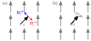
Figure 1: Illustration of (a) the constraining field $\mathbf{B}_{i}^{\text{con}}$ canceling the effective field $\mathbf{B}_{i}^{\text{eff}}$ and (b) of the finite error between the actual moment direction $\mathbf{m}_{i}$ and the prescribed direction $\mathbf{e}_{i}$ in the case without constraining field.

For the calculation of $E(\{\mathbf{e}_{i}\})$ from the electronic degrees of freedom, it is required to fix the moment directions in some way, as otherwise a self-consistent calculation would relax back to the ground state or a metastable state. An arbitrary moment configuration can be enforced exactly by adding a constraining field to the Hamiltonian [23, 24],

$$\hat{\mathcal{H}}_{\text{con}}=-\sum_{i}\hat{\mathbf{M}}_{i}\cdot\mathbf{B}_{i}^{\text{con}},$$ (3)

where $\hat{\mathbf{M}}_{i}$ is the total magnetic moment operator at site $i$ and $\mathbf{B}_{i}^{\text{con}}$ only constrains the moment directions and not their lengths, i.e., $\mathbf{B}_{i}^{\text{con}}\cdot\mathbf{e}_{i}=0$. The moment lengths $M_{i}$ are outputs of the self-consistent calculation for a given moment configuration, which implies that the energy is minimized with respect to the moment lengths. The effective field is given by the negative of the constraining field, see Fig. 1(a),

$$\mathbf{B}_{i}^{\text{eff}}=-\mathbf{B}_{i}^{\text{con}},$$ (4)

which is however not exactly valid in the case of DFT [36, 37]. For recent discussions of adiabatic spin dynamics based on the constraining field, we refer to Refs. [38, 35].

For DFT and mean-field theories, the moment directions can also be changed in an approximate way without constraining field. This can be illustrated by considering the following mean-field Stoner term,

$$\hat{\mathcal{H}}_{\text{St}}=-\frac{1}{2}\sum_{i}I\mathbf{M}_{i}\cdot\hat{\mathbf{M}}_{i},$$ (5)

with Stoner parameter $I$ (in units of $\text{eV}/\mu_{B}^{2}$) and $\mathbf{M}_{i}=\langle\hat{\mathbf{M}}_{i}\rangle$. In this self-consistent formulation, there is no information contained on the moment directions $\{\mathbf{e}_{i}\}$. However, we can write

$$\mathbf{M}_{i}=M_{i}\mathbf{e}_{i},$$ (6)

and keep the moment directions in Eq. (5) fixed. This will result in output moment directions $\mathbf{m}_{i}=\langle\hat{\mathbf{M}}_{i}\rangle/M_{i}\approx\mathbf{e}_{i}$, which are approximately aligned along the enforced moment direction $\mathbf{e}_{i}$ [39], even without a constraining field, see Fig. 1(b). Within this approximate approach, the Hamiltonian becomes dependent on the moment directions, $\hat{\mathcal{H}}=\hat{\mathcal{H}}(\{\mathbf{e}_{i}\})$. The effective field is then

$$\mathbf{B}_{i}^{\text{eff}}=-\frac{1}{M_{i}}\left\langle\boldsymbol{\nabla}_{\mathbf{e}_{i}}\hat{\mathcal{H}}\right\rangle,$$ (7)

which is equivalent to the magnetic force theorem in DFT [22] and is the basis of the LKAG formalism [21, 22, 40].

II.2 Energy curvature tensor

For the calculation of adiabatic magnon spectra the central quantity is the energy curvature tensor [34, 35],

$$\mathcal{J}_{ij}^{\alpha\beta}=-\frac{\partial^{2}E}{\partial e_{i}^{\alpha}\partial e_{j}^{\beta}},$$ (8)

with Cartesian components $\alpha,\beta\in\{x,y,z\}$. Here it is important to take into account that we are dealing with unit vectors, $|\mathbf{e}_{i}|=1$, and the derivatives in Eq. (8) actually represent rotations and not standard derivatives. We denote the corresponding quantity with standard derivatives by $\tilde{\mathcal{J}}_{ij}^{\alpha\beta}$. This subtlety has the consequence that the exchange tensor $J_{ij}^{\alpha\beta}$ of a tensorial Heisenberg model cannot be equated to the energy curvature tensor $\mathcal{J}_{ij}^{\alpha\beta}$ [35], instead $J_{ij}^{\alpha\beta}$ has to be extracted from $\mathcal{J}_{ij}^{\alpha\beta}$ in different magnetic configurations, which is straightforward in the collinear case [41, 42]. For a method to extract an isotropic Heisenberg interaction $J_{ij}$ from $\mathcal{J}_{ij}^{\alpha\beta}$ for non-collinear states, see Ref. [35]. In the following we consider the energy curvature tensor $\mathcal{J}_{ij}^{\alpha\beta}$ and not an exchange tensor $J_{ij}^{\alpha\beta}$.

The energy curvature tensor based on the constraining field is given by [34]

$$\mathcal{J}_{\mathrm{c},ij}^{\alpha\beta}=-\frac{\partial(M_{i}B_{i\alpha}^{\text{con}})}{\text{{\hbox{\partial e_{j}^{\beta}}}}},$$ (9)

for which explicit formulas have been derived previously [28, 30, 34]. The energy curvature tensor in the constraining field approach can be related to the inverse of the static magnetic susceptibility [27, 28, 29, 31, 30, 34],

$$\mathcal{\tilde{J}}_{\text{c},ij}^{\alpha\beta}=-\left[M_{i}^{-1}M_{j}^{-1}\chi_{ij}^{\alpha\beta}(0)\right]^{-1},$$ (10)

with

$$\chi_{ij}^{\alpha\beta}(0)=\frac{\partial M_{i}^{\alpha}}{\partial B_{j\beta}^{\text{con}}}.$$ (11)

In the framework of the MFT [21, 22, 40], the LKAG expression for the energy curvature tensor without constraining field is given by [40, 34],

$$\mathcal{\tilde{J}}_{\text{L},ij}^{\alpha\beta}=-\int_{\omega}\text{Tr}\left\{\frac{\partial\Sigma}{\partial e_{i}^{\alpha}}\mathcal{G}(i\omega)\frac{\partial\Sigma}{\partial e_{j}^{\beta}}\mathcal{G}(i\omega)\right\},$$ (12)

where $\mathcal{G}(i\omega)$ is the electron Green’s function, $\Sigma$ the self-energy, the trace is over electronic states, and the summation over Matsubara frequencies $\int_{\omega}=k_{B}T\sum_{\omega}$ [40, 34]. In the model that we are going to consider, the self-energy term is simply given by the Stoner term, Eq. (5).

In both expressions, Eq. (10) and (12), the tilde indicates that they have been derived without the constraint to unit length. The correct $\mathcal{J}_{ij}^{\alpha\beta}$ can be obtained from $\mathcal{\tilde{J}}_{ij}^{\alpha\beta}$ via the projection algorithm provided in Appendix A. This complication can be avoided by using spherical coordinates [41], which we do not consider here for the calculation of the energy curvature tensor.

II.3 Quantization

Given the energy curvature tensor $\mathcal{J}_{ij}^{\alpha\beta}$, small fluctuations around a stable magnetic configuration can be expressed in terms of a “local” energy variation [34],

$$\delta E_{\text{loc}}=-\frac{1}{2}\sum_{ij}\sum_{\alpha\beta}\mathcal{J}_{ij}^{\alpha\beta}\delta e_{i}^{\alpha}\delta e_{j}^{\beta},$$ (13)

where the vectors $\delta\mathbf{e}_{i}$ are transverse fluctuations of the moment directions (longitudinal fluctuations are not considered in this work). Since we are considering a stable configuration, $\mathcal{J}_{ij}^{\alpha\beta}$ must be negative semidefinite .

We derive the adiabatic magnon spectrum from this local energy by expanding the transverse fluctuations in spherical coordinates,

$$\delta\mathbf{e}_{i}=\delta e_{i}^{\theta}\mathbf{e}_{\theta_{i}}+\delta e_{i}^{\phi}\mathbf{e}_{\phi_{i}},$$ (14)

where $\mathbf{e}_{\theta_{i}}$ and $\mathbf{e}_{\phi_{i}}$ are unit vectors in the $\theta_{i}$ and $\phi_{i}$ directions, respectively, which are transverse to the moment direction $\mathbf{e}_{i}$. We quantize these fluctuations via the Holstein-Primakoff transformation to linear order,

$$\delta e_{i}^{\theta} \rightarrow\sqrt{\frac{1}{2S_{i}}}\left(\hat{b}_{i}^{\dagger}+\hat{b}_{i}\right),$$ (15)

$$\delta e_{i}^{\phi} \rightarrow-\mathrm{i}\sqrt{\frac{1}{2S_{i}}}\left(\hat{b}_{i}^{\dagger}-\hat{b}_{i}\right),$$ (16)

where the dimensionless spin number $S_{i}=M_{i}/(g\mu_{B})$ with $g=2$. The bosonic creation and annihilation operators fulfill the standard commutation relations,

$$[\hat{b}_{i},\hat{b}_{j}^{\dagger}]=\delta_{ij},\;[\hat{b}_{i},\hat{b}_{j}]=[\hat{b}_{i}^{\dagger},\hat{b}_{j}^{\dagger}]=0.$$ (17)

This results in the following local spin Hamiltonian,

$$\hat{\mathcal{H}}_{\mathrm{loc}}=\sum_{ij}\left(A_{ij}\hat{b}_{i}^{\dagger}\hat{b}_{j}+\frac{B_{ij}^{*}}{2}\hat{b}_{i}\hat{b}_{j}+\frac{B_{ij}}{2}\hat{b}_{i}^{\dagger}\hat{b}_{j}^{\dagger}\right),$$ (18)

where

$$A_{ij} =-\frac{1}{4}\sqrt{\frac{1}{S_{i}S_{j}}}\sum_{\alpha\beta}\left(\mathcal{J}_{ij}^{\alpha\beta}+\mathcal{J}_{ji}^{\beta\alpha}\right)$$

$$\times\left(e_{\theta_{i}}^{\alpha}e_{\theta_{j}}^{\beta}+\mathrm{i}e_{\theta_{i}}^{\alpha}e_{\phi_{j}}^{\beta}-\mathrm{i}e_{\phi_{i}}^{\alpha}e_{\theta_{j}}^{\beta}+e_{\phi_{i}}^{\alpha}e_{\phi_{j}}^{\beta}\right),$$ (19)

$$B_{ij} =-\frac{1}{4}\sqrt{\frac{1}{S_{i}S_{j}}}\sum_{\alpha\beta}\left(\mathcal{J}_{ij}^{\alpha\beta}+\mathcal{J}_{ji}^{\beta\alpha}\right)$$

$$\times\left(e_{\theta_{i}}^{\alpha}e_{\theta_{j}}^{\beta}-\mathrm{i}e_{\theta_{i}}^{\alpha}e_{\phi_{j}}^{\beta}-\mathrm{i}e_{\phi_{i}}^{\alpha}e_{\theta_{j}}^{\beta}-e_{\phi_{i}}^{\alpha}e_{\phi_{j}}^{\beta}\right),$$ (20)

with unit vectors

$$\mathbf{e}_{\theta_{i}}=\begin{pmatrix}\cos\theta_{i}\cos\phi_{i}\\ \cos\theta_{i}\sin\phi_{i}\\ -\sin\theta_{i}\end{pmatrix},\quad\mathbf{e}_{\phi_{i}}=\begin{pmatrix}-\sin\phi_{i}\\ \cos\phi_{i}\\ 0\end{pmatrix}.$$ (21)

Only the symmetric part, $(\mathcal{J}_{ij}^{\alpha\beta}+\mathcal{J}_{ji}^{\beta\alpha})/2$, of the energy curvature tensor enters in Eq. (18), which is consistent with the fact that energy curvature tensor can always be symmetrized within the energy given by Eq. (13). Considering the definition in Eq. (8), it might be expected that $\mathcal{J}_{ij}^{\alpha\beta}=\mathcal{J}_{ji}^{\beta\alpha}$, which is indeed true for $i\neq j$. However, since we are dealing with infinitesimal rotations instead of standard derivatives, the on-site term $\mathcal{J}_{ii}^{\alpha\beta}$ does not have to be symmetric because two rotations of the same moment do not commute beyond linear order.

In general, the magnon spectrum can now be obtained by diagonalizing the quadratic bosonic Hamiltonian, Eq. (18), with standard methods [44, 45]. In the case of translational invariance, diagonalization is achieved by Fourier and Bogoliubov transformations. For one magnetic moment per unit cell, the magnon dispersion is given by

$$\omega_{\mathbf{k}}=\sqrt{A_{\mathbf{k}}^{2}-|B_{\mathbf{k}}|^{2},}$$ (22)

with

$$A_{ij} =\frac{1}{N}\sum_{\mathbf{k}}A_{\mathbf{k}}e^{\text{i}\mathbf{k}\cdot(\mathbf{R}_{i}-\mathbf{R}_{j})},$$ (23)

$$B_{ij} =\frac{1}{N}\sum_{\mathbf{k}}B_{\mathbf{k}}e^{\text{i}\mathbf{k}\cdot(\mathbf{R}_{i}-\mathbf{R}_{j})},$$ (24)

$$B_{ij}^{*} =\frac{1}{N}\sum_{\mathbf{k}}B_{\mathbf{k}}^{*}e^{-\text{i}\mathbf{k}\cdot(\mathbf{R}_{i}-\mathbf{R}_{j})}.$$ (25)

where $N$ is the number of unit cells and $\mathbf{R}_{i}$ the corresponding lattice vectors. Here, $A_{\mathbf{k}}$ is a real-valued function due to the required Hermiticity of the Hamiltonian, Eq. (18), which implies $A_{ij}=A_{ji}$.

II.4 Ferromagnetic Heisenberg model

To demonstrate this general formalism for calculating the adiabatic magnon spectrum, we consider the case that the energy is described by the Heisenberg model,

$$E=-\frac{1}{2}\sum_{ij}J_{ij}\mathbf{e}_{i}\cdot\mathbf{e}_{j},$$ (26)

with a ferromagnetic ground state with all magnetic moments aligned along the $z$ axis. We set $J_{ii}=0$, since this would only give an irrelevant constant energy contribution. The energy curvature tensor is then given by

$$\mathcal{J}_{ij}^{\alpha\beta} \overset{i\neq j}{=}\begin{pmatrix}J_{ij}&0&0\\ 0&J_{ij}&0\\ 0&0&0\end{pmatrix}^{\alpha\beta},$$ (27)

$$\mathcal{J}_{ii}^{\alpha\beta} =\begin{pmatrix}-\sum_{j}J_{ij}&0&0\\ 0&-\sum_{j}J_{ij}&0\\ 0&0&0\end{pmatrix}^{\alpha\beta}.$$ (28)

The finite on-site contribution follows from the constraint to unit vectors, which leads to an energy curvature tensor different from the case without the constraint, $\tilde{\mathcal{J}}_{ij}^{\alpha\beta}=\delta_{ij}\delta^{\alpha\beta}J_{ij}$, see Appendix A on how to obtain $\mathcal{J}_{ij}^{\alpha\beta}$ from $\tilde{\mathcal{J}}_{ij}^{\alpha\beta}$. The on-site term $\mathcal{J}_{ii}^{xx}=\mathcal{J}_{ii}^{yy}=-\sum_{j}J_{ij}$ corresponds to the LKAG sum rule [22, 40, 25].

Quantizing the local spin Hamiltonian with the $\mathcal{J}_{ij}^{\alpha\beta}$ given above for a ferromagnetic ground state results in

$$\hat{\mathcal{H}}=-\sum_{ij}\frac{1}{\sqrt{S_{i}S_{j}}}J_{ij}\left(\hat{b}_{i}^{\dagger}\hat{b}_{j}-\hat{b}_{i}^{\dagger}\hat{b}_{i}\right).$$ (29)

This is to quadratic order exactly equivalent to directly quantizing the Heisenberg model given in Eq. (26) without mapping to the local spin Hamiltonian. In the case of the local spin Hamiltonian the on-site contribution $\hat{b}_{i}^{\dagger}\hat{b}_{i}$ comes from $\mathcal{J}_{ii}^{\alpha\beta}$, whereas when directly quantizing the Heisenberg model it comes from the quantization of the longitudinal component, $e_{i}^{z}=1-\hat{b}_{i}^{\dagger}\hat{b}_{i}/S_{i}$, which is not present in the local spin Hamiltonian.

Assuming translational invariance with $S_{i}=S$ and

$$J_{ij}=J(\mathbf{R}_{i}-\mathbf{R}_{j})=\frac{1}{N}\sum_{\mathbf{k}}J_{\mathbf{k}}e^{\mathrm{i}\mathbf{k}\cdot(\mathbf{R}_{i}-\mathbf{R}_{j})},$$ (30)

the magnon dispersion is given by

$$\omega_{\mathbf{k}}=-\frac{1}{S}(J_{\mathbf{k}}-J_{0}).$$ (31)

In the following, we will consider ferromagnetic atomic chains with periodic boundary conditions and without spin-orbit coupling. For these systems, small fluctuations around the ferromagnetic ground state are exactly described by the Heisenberg model [22] and the energy curvature tensor $\mathcal{J}_{ij}^{\alpha\beta}$ takes the form given by Eqs. (27-28). Therefore, in these cases the adiabatic magnon dispersion is simply given by Eq. (31).

III Mean-field Stoner model

To benchmark different methods for the adiabatic magnon spectrum, we need an exactly solvable model for which we can obtain the exact spectrum from the dynamic magnetic susceptibility. We introduce in Sec. III.1 therefore an exactly solvable tight-binding model with a mean-field Stoner term and derive in Sec. III.2 the corresponding magnetic susceptibility.

III.1 Tight-binding model

We consider a tight-binding model with a mean-field Stoner term,

$$\hat{\mathcal{H}}_{\mathrm{tb}}=\hat{\mathcal{H}}_{0}+\hat{\mathcal{H}}_{\text{St}}.$$ (32)

The hopping part is given by

$$\hat{\mathcal{H}}_{0}=\sum_{i\ell,j\ell^{\prime},\sigma}t_{i\ell,j\ell^{\prime}}\hat{c}_{i\ell\sigma}^{\dagger}\hat{c}_{j\ell^{\prime}\sigma},$$ (33)

where $t_{i\ell,j\ell^{\prime}}$ is the hopping matrix element from the orbital $\ell^{\prime}$ at lattice site $j$ to the orbital $\ell$ at lattice site $i$ and $\hat{c}_{i\ell\sigma}^{\dagger}$ and $\hat{c}_{j\ell^{\prime}\sigma}$ are the corresponding creation and annihilation operators with electron spin $\sigma\in\{\uparrow,\downarrow\}$. For simplicity we consider only $d$ orbitals. The Stoner term is then given by

$$\hat{\mathcal{H}}_{\text{St}} =-\frac{1}{2}\sum_{i}I\mathbf{M}_{i}\cdot\hat{\mathbf{M}}_{i},$$ (34)

where $I$ is the Stoner parameter and $\hat{\mathbf{M}}_{i}$ the total magnetic moment operator at site $i$ (summed over all orbitals $\ell$) with expectation value $\mathbf{M}_{i}=\langle\hat{\mathbf{M}}_{i}\rangle$. The restriction to $d$ orbitals allows us to consider only a single Stoner parameter $I$ for the $d$ orbitals and to consider only the total magnetic moment $\mathbf{M}_{i}$ instead of having to deal with separate orbital contributions $\mathbf{M}_{i\ell}$, simplifying the analysis of exchange parameters and magnetic susceptibility.

We emphasize that we consider here the Hamiltonian $\hat{\mathcal{H}}_{\mathrm{tb}}$ in Eq. (32) as our reference point, with a spin-pairing energy given by the mean-field expression of Eq. (34). This is a simplification of a more general expression, where the Stoner interaction would be given by

$$\hat{\mathcal{H}}_{\text{int}}=-\frac{1}{4}\sum_{i}I\hat{\mathbf{M}}_{i}\cdot\hat{\mathbf{M}}_{i}.$$ (35)

The reason for this simplification is that we want to benchmark the adiabatic approximation for an exactly solvable model. We do not aim to compare different approximations to the interaction term (35), which cannot be solved exactly in a straightforward way. When we refer to the exact magnon spectrum, we refer to the spectrum of the tight-binding mean-field model $\hat{\mathcal{H}}_{\mathrm{tb}}$ and not to a more fundamental Hamiltonian to which $\hat{\mathcal{H}}_{\mathrm{tb}}$ would be an approximation.

III.2 Dynamic magnetic susceptibility

The dynamic magnetic susceptibility $\chi_{ij}^{\alpha\beta}(t)$ is the magnetic response to an external magnetic field $\mathbf{B}_{i}(t)$,

$$\delta\left\langle\hat{M}_{i}^{\alpha}(t)\right\rangle=\sum_{j\beta}\int\mathrm{d}t^{\prime}\,\chi_{ij}^{\alpha\beta}(t-t^{\prime})B_{j}^{\beta}(t^{\prime}).$$ (36)

In the limit of a weak magnetic field, this response can be obtained from linear response theory [1, 46].

We first consider the case of non-interacting electrons without a mean-field term,

$$\hat{\mathcal{H}}_{0}(t)=\hat{\mathcal{H}}_{0}+\hat{V}(t),$$ (37)

with perturbation

$$\hat{V}(t)=-\sum_{i}\hat{\mathbf{M}}_{i}\cdot\mathbf{B}_{i}(t).$$ (38)

The bare dynamic magnetic susceptibility is in linear response given by [1]

$$\chi_{0,ij}^{\alpha\beta}(t-t^{\prime})=\frac{\text{i}}{\hbar}\theta(t-t^{\prime})\left\langle\left[\hat{M}_{i}^{\alpha}(t),\hat{M}_{j}^{\beta}(t^{\prime})\right]\right\rangle.$$ (39)

Fourier transforming to the frequency domain and expanding in the eigenbasis $\{\ket{n}\}$ with energies $E_{n}$, we get

$$\chi_{0,ij}^{\alpha\beta}(\omega) =-\sum_{n,m}f(E_{n})\left\{\frac{\braket{n}{\hat{M}_{i}^{\alpha}}{m}\braket{m}{\hat{M}_{j}^{\beta}}{n}}{\omega+(E_{n}-E_{m})+\mathrm{i}\eta}\right.$$

$$\phantom{-\sum_{n,m}f(E_{n})\quad\;}\left.-\frac{\braket{m}{\hat{M}_{i}^{\alpha}}{n}\braket{n}{\hat{M}_{j}^{\beta}}{m}}{\omega-(E_{n}-E_{m})+\mathrm{i}\eta}\right\},$$ (40)

where $f(E_{n})$ is the Fermi distribution function and the infinitesimal positive imaginary term $\mathrm{i}\eta$ with $\eta\to 0^{+}$ is required for convergence and results from the Fourier transform of $\theta(t-t^{\prime})$.

In our mean-field model, we have to take into account the time dependence of the Stoner term, Eq. (34), which results in an additional perturbation,

$$\delta\hat{\mathcal{H}}_{\text{St}}(t)=-\frac{1}{2}\sum_{i}I\delta\mathbf{M}_{i}(t)\cdot\hat{\mathbf{M}}_{i}.$$ (41)

Expressing the time-dependent perturbation of the magnetic moments via the full susceptibility $\chi_{ij}^{\alpha\beta}$,

$$\delta M_{i}^{\alpha}(t)=\sum_{j\beta}\int\text{d}t^{\prime}\,\chi_{ij}^{\alpha\beta}(t-t^{\prime})B_{j}^{\beta}(t^{\prime}),$$ (42)

the effective perturbation is given by

$$\hat{V}_{\text{eff}}(t) =-\sum_{i\alpha}\sum_{j\beta}\int\text{d}t^{\prime}\,\left[\delta_{ij}^{\alpha\beta}\delta(t-t^{\prime})+\frac{1}{2}I\chi_{ij}^{\alpha\beta}(t-t^{\prime})\right]$$

$$\phantom{=-\sum_{i\alpha}\sum_{j\beta}\int\text{d}t^{\prime}\,}\times B_{j}^{\beta}(t^{\prime})\hat{M}_{i}^{\alpha},$$ (43)

resulting in the following equation for the susceptibility,

$$\chi_{\mathbf{k}}^{\alpha\beta}(\omega)=\chi_{0,\mathbf{k}}^{\alpha\beta}(\omega)+\frac{1}{2}I\sum_{\nu}\chi_{0,\mathbf{k}}^{\alpha\nu}(\omega)\chi_{\mathbf{k}}^{\nu\beta}(\omega),$$ (44)

with

$$\chi_{ij}^{\alpha\beta}(\omega)=\frac{1}{N}\sum_{\mathbf{k}}\chi_{\mathbf{k}}^{\alpha\beta}(\omega)e^{\mathrm{i}\mathbf{k}\cdot(\mathbf{R}_{i}-\mathbf{R}_{j})}.$$ (45)

In the ferromagnetic and isotropic case with $\chi_{\mathbf{k}}^{xx}=\chi_{\mathbf{k}}^{yy}$ and $\chi_{\mathbf{k}}^{xy}=\chi_{\mathbf{k}}^{yx}$ (and $\chi_{\mathbf{k}}^{xz}=\chi_{\mathbf{k}}^{zx}=\chi_{\mathbf{k}}^{yz}=\chi_{\mathbf{k}}^{zy}=0$), the transverse magnetic susceptibility in the $\pm$ basis (with $M_{\mathbf{k}}^{\pm}=M_{\mathbf{k}}^{x}\pm\mathrm{i}M_{\mathbf{k}}^{y}$) is given by [5]

$$\chi_{\mathbf{k}}^{\pm}=\chi_{\mathbf{k}}^{xx}\mp\mathrm{i}\chi_{\mathbf{k}}^{xy}.$$ (46)

We obtain the familiar random phase approximation (RPA) expression for the magnetic susceptibility [31, 25],

$$\chi_{\mathbf{k}}^{\pm}(\omega)=\frac{\chi_{0,\mathbf{k}}^{\pm}(\omega)}{1-\frac{I}{2}\chi_{0,\mathbf{k}}^{\pm}(\omega)}.$$ (47)

The magnon spectrum is then obtained from the low-energy peaks of $\text{Im}\,\chi_{\mathbf{k}}^{\pm}(\omega)$, which are at positive frequencies for $\chi^{+}$ and at at negative frequencies for $\chi^{-}$.

IV Numerical results

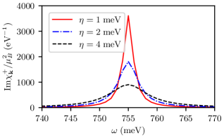
Figure 2: Effect of the imaginary part $\eta$ in Eq. (40) on the magnon linewidth for $I\mu_{B}^{2}=1\;\text{eV}$ at $k=\pi/a$.

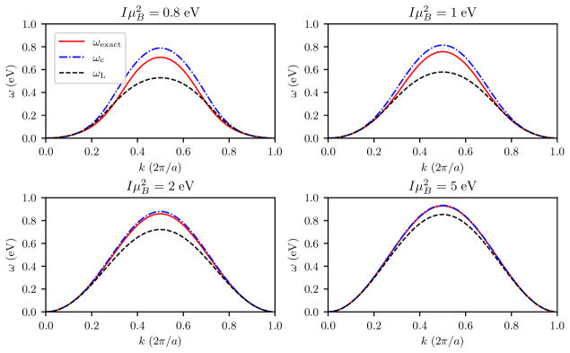
Figure 3: Comparison of the exact magnon spectrum ($\omega_{\text{exact}}$) with adiabatic magnon spectra obtained with constraining field ($\omega_{\text{c}}$) and the LKAG formalism without constraining field ($\omega_{\text{L}}$) for various Stoner parameters $I\mu_{B}^{2}$ from $0.8\;\text{eV}$ to $5\;\text{eV}$.

In this section, we present a comparison of adiabatic and exact magnon spectra for the mean-field model given in Sec. III. The calculations are performed in the zero temperature limit with the tight-binding electronic structure implementation of the code CAHMD [47] for an atomic chain with lattice parameter $a$ and periodic boundary conditions consisting of $64$ atoms with nearest neighbor hopping parameters of bulk bcc Fe [48] (i.e., $a\approx 2.5\;\mathring{\mathrm{A}}$), resulting in a magnetic moment length of $M=2\mu_{B}$. The key property of this model is the tunability of the Stoner parameter $I$, which we can adjust in a wide range from non-adiabatic (weak-coupling) to adiabatic (strong-coupling) regimes. A typical value for transition metal magnets is $I=1\;\text{eV}/\mu_{B}^{2}$ [49, 50, 51]. For the numerical calculation of the bare susceptibility $\chi_{0,ij}^{\alpha\beta}(\omega)$, Eq. (40), we use a frequency spacing $\delta\omega=1\;\text{meV}$ and an imaginary part $\eta=1\;\text{meV}$. The magnon lineshape is shown in Fig. 2 for several values of $\eta$, which demonstrates that we can extract the magnon peak from our numerical calculations with our choice of parameters and that the broadening of the peaks is determined by $\eta$ and therefore artificial. A notable feature of our mean-field model is the absence of any Landau damping [5], which would broaden the magnon peaks. The reason is that we only take $d$ orbitals into account, for which the Stoner spin-flip excitations are at higher energies than the magnon energies. In a more realistic model, spin-flip excitations from $s$ and $p$ orbitals would fall within the range of magnon energies, causing Landau damping.

The main results of this article are presented in Fig. 3, where we compare the adiabatic magnon spectra with ($\omega_{\text{c}}$) and without ($\omega_{\text{L}}$) constraining field with the exact spectrum ($\omega_{\text{exact}}$) for several values of the Stoner coupling $I$. These magnon spectra hence derive from the Heisenberg exchange parameters from Eqs. (10) and (12), combined with adiabatic spin-wave theory, to evaluate the magnon dispersion. These results are compared to the exact results evaluated from Eq. (47). We find that the constraining field results perform in general better than the LKAG results for high magnon energies and also in the strong coupling regime ($I\mu_{B}^{2}\gtrsim 1\;\mathrm{eV}$), while the LKAG results are in better agreement with the exact spectrum for low magnon energies in the weak coupling regime ($I\mu_{B}^{2}\lesssim 1\;\mathrm{eV}$). The constraining field results tend to overestimate magnon energies, whereas the LKAG results tend to underestimate them. This is similar to a previous comparison for bulk fcc Ni [5], where it was found that the constraining field improves the agreement with the exact result, although with a slight underestimation at lower magnon energies and an overestimation only at higher magnon energies.

Our numerical results for the adiabatic magnon energies $\omega_{\text{c}}$ and $\omega_{\text{L}}$ fulfill exactly the relation [28]

$$\omega_{\text{c}}(\mathbf{k})=\frac{\omega_{\text{L}}(\mathbf{k})}{1-\omega_{\text{L}}(\mathbf{k})/\Delta},$$ (48)

where the exchange splitting $\Delta=\mu_{B}MI$ is determined by the product of the moment length (here, $M=2\mu_{B}$) and Stoner coupling $I$. This is not surprising since the approximations that were made to derive this relation in Ref. [28] are exactly fulfilled for our model. This simple relation shows that $\omega_{\text{c}}$ and $\omega_{\text{L}}$ agree in the limit $\omega\ll\Delta$, as is expected [28, 29, 31]. Furthermore, Eq. (48) shows that $\omega_{\mathrm{c}}>\omega_{\mathrm{L}}$, which can be explained from the fact that the constraining field enforces the spin configuration without the relaxation to a lower energy configuration that is allowed by the LKAG approach.

V Summary and Discussion

We have compared in this work two different implementations of the adiabatic magnon spectrum with the exact spectrum of an exactly solvable mean-field model. While both methods are equally valid in the limit of magnon energies much smaller than the exchange splitting, $\omega\ll\Delta$, we find that adiabatic magnon spectra with constraining field are more accurate at high magnon energies and strong Stoner coupling in comparison with the LKAG method without constraining field, whereas the LKAG method performs better at low magnon energies in the case of weak Stoner coupling. Furthermore, we have presented a general formalism to obtain the adiabatic magnon spectrum from the energy curvature tensor, which is applicable for any non-collinear ground state. The projection algorithm provided in Appendix. A simplifies the calculation of the energy curvature tensor since the constraint to unit length can be disregarded initially.

For the comparison of ab initio magnon spectra with experimental data, we have to consider that the calculations already include approximations on the electronic structure level. Therefore, when comparing adiabatic magnon spectra with and without constraining field with experimental data, we are not only evaluating the quality of the adiabatic approximations itself but instead a combination of electronic structure approximations and adiabatic approximations. In this work, we have only compared adiabatic magnon spectra for an exactly solvable mean-field model. One could consider this mean-field model as an approximation to a more fundamental interacting model and ask the question which implementation of the adiabatic approximation in combination with the mean-field approximation performs better in comparison with the exact spectrum of the more fundamental model. However, this is beyond the scope of the present work. If there is a cancellation of errors between mean-field and adiabatic approximations, this could lead to contrary conclusions than we have drawn by considering the adiabatic approximation by itself. A previously discussed example of such a cancellation of errors is fcc Ni, for which the adiabatic magnon spectrum without constraining field is in better agreement with experimental data than the spectrum with constraining field [31], although the spectrum with constraining field is in better agreement with the magnon spectrum obtained from TDDFT [5]. These observations have been attributed to an overestimation of the exchange splitting and magnon energies for fcc Ni in TDDFT (within the adiabatic local spin density approximation), which are compensated by an underestimation of magnon energies by the adiabatic magnon spectrum without constraining field [27, 5, 11, 12]. Therefore, we emphasize that when comparing different implementations of the adiabatic magnon spectrum, the best reference is the magnon spectrum without adiabatic approximation calculated within the same electronic structure description, since comparisons with experimental data can be misleading due to errors introduced already by approximations of the electronic structure.

While we have considered here an exactly solvable, but simplified, model, further comparisons of adiabatic magnon spectra with and without constraining field with the TDDFT magnon spectrum have been planned for the future by the authors of Ref. [12], which will address this issue for magnetic materials besides fcc Ni [5]. For the case of fcc Ni, it would also be of interest to compare adiabatic magnon spectra with the magnon spectrum in an approach where the exchange splitting is reduced by a factor of two to better agree with experiments [52], or more generally, with approaches that are better suited for the strong electron correlations in fcc Ni [53, 54, 55, 56, 33]. In cases where there is a significant difference between adiabatic and exact magnon spectra, it could be advantageous to perform spin dynamics simulations with exchange parameters that reproduce the exact magnon spectrum, as was proposed already in Ref. [7] for the description of the ferromagnetic resonance.

Appendix A Projection algorithm

When calculating the energy curvature tensor,

$$\mathcal{J}_{ij}^{\alpha\beta}=-\frac{\partial^{2}E}{\partial e_{i}^{\alpha}\partial e_{j}^{\beta}},$$ (49)

it is crucial to take into account that we are dealing with rotations of unit vectors [35]. However, when working in Cartesian coordinates, it may be more convenient to first disregard this constraint to unit length and work with standard derivatives. In a second step, the unphysical contributions can then be projected out [34]. We present here a method to perform this projection to transverse fluctuations of the unit vectors $\mathbf{e}_{i}$ and $\mathbf{e}_{j}$.

We will perform the projection in two steps. For the first derivative of the energy, we have

$$\boldsymbol{\nabla}_{\mathbf{e}_{i}}E =\tilde{\boldsymbol{\nabla}}_{\mathbf{e}_{i}}E-\mathbf{e}_{i}\left(\mathbf{e}_{i}\cdot\tilde{\boldsymbol{\nabla}}_{\mathbf{e}_{i}}E\right),$$ (50)

where $\tilde{\boldsymbol{\nabla}}_{\mathbf{e}_{i}}$ denotes the unconstrained gradient. The constraint to unit vectors simply eliminates the parallel component of the gradient. Taking now the second derivative without constraint, we obtain the partially constrained curvature tensor,

$$\tilde{\mathcal{J}}_{i_{\perp}j}^{\alpha\beta}=\tilde{\mathcal{J}}_{ij}^{\alpha\beta}-\sum_{\nu}\tilde{\mathcal{J}}_{ij}^{\nu\beta}e_{i}^{\nu}e_{i}^{\alpha}-\delta_{ij}M_{i}\left(e_{i}^{\alpha}\tilde{B}_{i}^{\beta}+\delta^{\alpha\beta}\mathbf{e}_{i}\cdot\tilde{\mathbf{B}}_{i}\right),$$ (51)

where $\tilde{\mathcal{J}}_{ij}^{\alpha\beta}$ denotes the unconstrained curvature tensor and $\tilde{\mathcal{J}}_{i_{\perp}j}^{\alpha\beta}$ is only constrained with respect to $\mathbf{e}_{i}$. The unconstrained effective field is defined by

$$\tilde{\mathbf{B}}_{i}=-\frac{1}{M_{i}}\tilde{\boldsymbol{\nabla}}_{\mathbf{e}_{i}}E,$$ (52)

which may contain a parallel contribution that can be finite even for a stable magnetic configuration where the perpendicular component has to vanish.

For the constraint on the second derivative, we have

$$\boldsymbol{\nabla}_{\mathbf{e}_{j}}\frac{\partial E}{\partial e_{i}^{\alpha}} =\tilde{\boldsymbol{\nabla}}_{\mathbf{e}_{j}}\frac{\partial E}{\partial e_{i}^{\alpha}}-\mathbf{e}_{j}\left(\mathbf{e}_{j}\cdot\tilde{\boldsymbol{\nabla}}_{\mathbf{e}_{j}}\frac{\partial E}{\partial e_{i}^{\alpha}}\right),$$ (53)

resulting in the proper energy curvature tensor,

$$\mathcal{J}_{ij}^{\alpha\beta}=\mathcal{\tilde{J}}_{i_{\perp}j}^{\alpha\beta}-\sum_{\nu}\tilde{\mathcal{J}}_{i_{\perp}j}^{\alpha\nu}e_{j}^{\nu}e_{j}^{\beta}.$$ (54)

References

- Marshall and Lowde [1968] W. Marshall and R. D. Lowde, Magnetic correlations and neutron scattering, Rep. Prog. Phys. 31, 705 (1968).
- Runge and Gross [1984] E. Runge and E. K. U. Gross, Density-functional theory for time-dependent systems, Phys. Rev. Lett. 52, 997 (1984).
- Gross and Kohn [1985] E. K. U. Gross and W. Kohn, Local density-functional theory of frequency-dependent linear response, Phys. Rev. Lett. 55, 2850 (1985).
- Savrasov [1998] S. Y. Savrasov, Linear Response Calculations of Spin Fluctuations, Phys. Rev. Lett. 81, 2570 (1998).
- Buczek et al. [2011] P. Buczek, A. Ernst, and L. M. Sandratskii, Different dimensionality trends in the Landau damping of magnons in iron, cobalt, and nickel: Time-dependent density functional study, Phys. Rev. B 84, 174418 (2011).
- Lounis et al. [2011] S. Lounis, A. T. Costa, R. B. Muniz, and D. L. Mills, Theory of local dynamical magnetic susceptibilities from the Korringa-Kohn-Rostoker Green function method, Phys. Rev. B 83, 035109 (2011).
- dos Santos Dias et al. [2015] M. dos Santos Dias, B. Schweflinghaus, S. Blügel, and S. Lounis, Relativistic dynamical spin excitations of magnetic adatoms, Phys. Rev. B 91, 075405 (2015).
- Wysocki et al. [2017] A. L. Wysocki, V. N. Valmispild, A. Kutepov, S. Sharma, J. K. Dewhurst, E. K. U. Gross, A. I. Lichtenstein, and V. P. Antropov, Spin-density fluctuations and the fluctuation-dissipation theorem in ferromagnetic metals, Phys. Rev. B 96, 184418 (2017).
- Cao et al. [2018] K. Cao, H. Lambert, P. G. Radaelli, and F. Giustino, Ab initio calculation of spin fluctuation spectra using time-dependent density functional perturbation theory, plane waves, and pseudopotentials, Phys. Rev. B 97, 024420 (2018).
- Tancogne-Dejean et al. [2020] N. Tancogne-Dejean, F. G. Eich, and A. Rubio, Time-Dependent Magnons from First Principles, J. Chem. Theory Comput. 16, 1007 (2020).
- Skovhus and Olsen [2021] T. Skovhus and T. Olsen, Dynamic transverse magnetic susceptibility in the projector augmented-wave method: Application to Fe, Ni, and Co, Phys. Rev. B 103, 245110 (2021).
- Durhuus et al. [2023] F. L. Durhuus, T. Skovhus, and T. Olsen, Plane wave implementation of the magnetic force theorem for magnetic exchange constants: application to bulk Fe, Co and Ni, J. Phys.: Condens. Matter 35, 105802 (2023).
- Gorni et al. [2022] T. Gorni, O. Baseggio, P. Delugas, S. Baroni, and I. Timrov, turboMagnon - A code for the simulation of spin-wave spectra using the Liouville-Lanczos approach to time-dependent density-functional perturbation theory, Comput. Phys. Commun. 280, 108500 (2022).
- Vishina et al. [2020] A. Vishina, O. Y. Vekilova, T. Björkman, A. Bergman, H. C. Herper, and O. Eriksson, High-throughput and data-mining approach to predict new rare-earth free permanent magnets, Phys. Rev. B 101, 094407 (2020).
- Frey et al. [2020] N. C. Frey, M. K. Horton, J. M. Munro, S. M. Griffin, K. A. Persson, and V. B. Shenoy, High-throughput search for magnetic and topological order in transition metal oxides, Sci. Adv. 6, eabd1076 (2020).
- Zhang [2021] H. Zhang, High-throughput design of magnetic materials, Electron. struct. 3, 033001 (2021).
- Vishina et al. [2023] A. Vishina, O. Eriksson, and H. C. Herper, Fe2C- and Mn2(W/Mo)B4-based rare-earth-free permanent magnets as a result of the high-throughput and data-mining search, Mater. Res. Lett. 11, 76 (2023).
- Antropov et al. [1995] V. P. Antropov, M. I. Katsnelson, M. van Schilfgaarde, and B. N. Harmon, Spin Dynamics in Magnets, Phys. Rev. Lett. 75, 729 (1995).
- Antropov et al. [1996] V. P. Antropov, M. I. Katsnelson, B. N. Harmon, M. van Schilfgaarde, and D. Kusnezov, Spin dynamics in magnets: Equation of motion and finite temperature effects, Phys. Rev. B 54, 1019 (1996).
- Halilov et al. [1998] S. V. Halilov, H. Eschrig, A. Y. Perlov, and P. M. Oppeneer, Adiabatic spin dynamics from spin-density-functional theory: Application to Fe, Co, and Ni, Phys. Rev. B 58, 293 (1998).
- Liechtenstein et al. [1984] A. I. Liechtenstein, M. I. Katsnelson, and V. A. Gubanov, Exchange interactions and spin-wave stiffness in ferromagnetic metals, J. Phys. F 14, L125 (1984).
- Liechtenstein et al. [1987] A. I. Liechtenstein, M. I. Katsnelson, V. P. Antropov, and V. A. Gubanov, Local spin density functional approach to the theory of exchange interactions in ferromagnetic metals and alloys, J. Magn. Magn. Mater. 67, 65 (1987).
- Stocks et al. [1998] G. M. Stocks, B. Ujfalussy, X. Wang, D. M. C. Nicholson, W. A. Shelton, Y. Wang, A. Canning, and B. L. Györffy, Towards a constrained local moment model for first principles spin dynamics, Philos. Mag. B 78, 665 (1998).
- Ujfalussy et al. [1999] B. Ujfalussy, X.-D. Wang, D. M. C. Nicholson, W. A. Shelton, G. M. Stocks, Y. Wang, and B. L. Gyorffy, Constrained density functional theory for first principles spin dynamics, J. Appl. Phys. 85, 4824 (1999).
- Szilva et al. [2022] A. Szilva, Y. Kvashnin, E. A. Stepanov, L. Nordström, O. Eriksson, A. I. Lichtenstein, and M. I. Katsnelson, Quantitative theory of magnetic interactions in solids (2022), arXiv:2206.02415 .
- Gorbatov et al. [2021] O. I. Gorbatov, G. Johansson, A. Jakobsson, S. Mankovsky, H. Ebert, I. Di Marco, J. Minár, and C. Etz, Magnetic exchange interactions in yttrium iron garnet: A fully relativistic first-principles investigation, Phys. Rev. B 104, 174401 (2021).
- Grotheer et al. [2001] O. Grotheer, C. Ederer, and M. Fähnle, Fast ab initio methods for the calculation of adiabatic spin wave spectra in complex systems, Phys. Rev. B 63, 100401 (2001).
- Bruno [2003] P. Bruno, Exchange interaction parameters and adiabatic spin-wave spectra of ferromagnets: A “renormalized magnetic force theorem”, Phys. Rev. Lett. 90, 087205 (2003).
- Antropov [2003] V. Antropov, The exchange coupling and spin waves in metallic magnets: removal of the long-wave approximation, J. Magn. Magn. Mater. 262, L192 (2003).
- Solovyev [2021] I. V. Solovyev, Exchange interactions and magnetic force theorem, Phys. Rev. B 103, 104428 (2021).
- Katsnelson and Lichtenstein [2004] M. I. Katsnelson and A. I. Lichtenstein, Magnetic susceptibility, exchange interactions and spin-wave spectra in the local spin density approximation, J. Phys. Condens. Matter 16, 7439 (2004).
- Jacobsson et al. [2022] A. Jacobsson, G. Johansson, O. I. Gorbatov, M. Ležaić, B. Sanyal, S. Blügel, and C. Etz, Efficient parameterisation of non-collinear energy landscapes in itinerant magnets, Sci. Rep. 12, 18987 (2022).
- Katanin et al. [2022] A. A. Katanin, A. S. Belozerov, A. I. Lichtenstein, and M. I. Katsnelson, Exchange interactions in iron and nickel: DFT+DMFT study in paramagnetic phase (2022), arXiv:2212.09267 .
- Streib et al. [2021] S. Streib, A. Szilva, V. Borisov, M. Pereiro, A. Bergman, E. Sjöqvist, A. Delin, M. I. Katsnelson, O. Eriksson, and D. Thonig, Exchange constants for local spin Hamiltonians from tight-binding models, Phys. Rev. B 103, 224413 (2021).
- Streib et al. [2022] S. Streib, R. Cardias, M. Pereiro, A. Bergman, E. Sjöqvist, C. Barreteau, A. Delin, O. Eriksson, and D. Thonig, Adiabatic spin dynamics and effective exchange interactions from constrained tight-binding electronic structure theory: Beyond the Heisenberg regime, Phys. Rev. B 105, 224408 (2022).
- Streib et al. [2020] S. Streib, V. Borisov, M. Pereiro, A. Bergman, E. Sjöqvist, A. Delin, O. Eriksson, and D. Thonig, Equation of motion and the constraining field in ab initio spin dynamics, Phys. Rev. B 102, 214407 (2020).
- Cai et al. [2022] Z. Cai, K. Wang, Y. Xu, and B. Xu, First-principles study of non-collinear spin fluctuations using self-adaptive spin-constrained method (2022), arXiv:2208.04551 .
- Cardias et al. [2021] R. Cardias, C. Barreteau, P. Thibaudeau, and C. C. Fu, Spin dynamics from a constrained magnetic tight-binding model, Phys. Rev. B 103, 235436 (2021).
- Singer et al. [2005] R. Singer, M. Fähnle, and G. Bihlmayer, Constrained spin-density functional theory for excited magnetic configurations in an adiabatic approximation, Phys. Rev. B 71, 214435 (2005).
- Katsnelson and Lichtenstein [2000] M. I. Katsnelson and A. I. Lichtenstein, First-principles calculations of magnetic interactions in correlated systems, Phys. Rev. B 61, 8906 (2000).
- Udvardi et al. [2003] L. Udvardi, L. Szunyogh, K. Palotás, and P. Weinberger, First-principles relativistic study of spin waves in thin magnetic films, Phys. Rev. B 68, 104436 (2003).
- Mankovsky and Ebert [2022] S. Mankovsky and H. Ebert, First-principles calculation of the parameters used by atomistic magnetic simulations, Electro. Struct. 4, 034004 (2022).
- Note [1] For a magnetically isotropic system, global rotations of all moment directions leave the energy invariant and may therefore have zero energy eigenvalues.
- Colpa [1978] J. Colpa, Diagonalization of the quadratic boson hamiltonian, Physica A 93, 327 (1978).
- Blaizot and Ripka [1986] J. P. Blaizot and G. Ripka, Quantum Theory of Finite Systems (MIT Press, Cambridge, Massachusetts, 1986).
- Kübler [2000] J. Kübler, Theory of Itinerant Electron Magnetism (Oxford University Press, Oxford, 2000).
- [47] Computer code CAHMD, classical atomistic hybrid multi-degree dynamics. A computer program package for atomistic dynamics simulations of multiple degrees of freedom (e.g. electron, magnetization, lattice vibrations) based on parametrized Hamiltonians. (Danny Thonig, danny.thonig@oru.se, 2013) (unpublished, available from https://cahmd.gitlab.io/cahmdweb/).
- Thonig and Henk [2014] D. Thonig and J. Henk, Gilbert damping tensor within the breathing Fermi surface model: anisotropy and non-locality, New J. Phys 16, 013032 (2014).
- Autès et al. [2006] G. Autès, C. Barreteau, D. Spanjaard, and M.-C. Desjonquères, Magnetism of iron: from the bulk to the monatomic wire, J. Phys. Condens. Matter 18, 6785 (2006).
- Barreteau et al. [2016] C. Barreteau, D. Spanjaard, and M.-C. Desjonquères, An efficient magnetic tight-binding method for transition metals and alloys, C. R. Phys. 17, 406 (2016).
- Rossen [2019] S. Rossen, Magnetization disorder at finite temperature: A tight-binding Monte Carlo modelling and spin dynamics study of bulk iron and cobalt clusters: theory, numerical implementation and simulations, Ph.D. thesis, Radboud University Nijmegen (2019).
- Müller et al. [2016] M. C. T. D. Müller, C. Friedrich, and S. Blügel, Acoustic magnons in the long-wavelength limit: Investigating the Goldstone violation in many-body perturbation theory, Phys. Rev. B 94, 064433 (2016).
- Lichtenstein et al. [2001] A. I. Lichtenstein, M. I. Katsnelson, and G. Kotliar, Finite-temperature magnetism of transition metals: An ab initio dynamical mean-field theory, Phys. Rev. Lett. 87, 067205 (2001).
- Sánchez-Barriga et al. [2012] J. Sánchez-Barriga, J. Braun, J. Minár, I. Di Marco, A. Varykhalov, O. Rader, V. Boni, V. Bellini, F. Manghi, H. Ebert, M. I. Katsnelson, A. I. Lichtenstein, O. Eriksson, W. Eberhardt, H. A. Dürr, and J. Fink, Effects of spin-dependent quasiparticle renormalization in Fe, Co, and Ni photoemission spectra:An experimental and theoretical study, Phys. Rev. B 85, 205109 (2012).
- Acharya et al. [2020] S. R. Acharya, V. Turkowski, G. P. Zhang, and T. S. Rahman, Ultrafast Electron Correlations and Memory Effects at Work: Femtosecond Demagnetization in Ni, Phys. Rev. Lett. 125, 017202 (2020).
- Nabok et al. [2021] D. Nabok, S. Blügel, and C. Friedrich, Electron–plasmon and electron–magnon scattering in ferromagnets from first principles by combining GW and GT self-energies, npj Comput. Mater. 7, 178 (2021).