Clumpy wind studies and the non-detection of cyclotron line in OAO 1657$-$415

Abstract

Winds of massive stars are suspected to be inhomogeneous (or clumpy), which biases the measures of their mass loss rates. In High Mass X-ray Binaries (HMXBs), the compact object can be used as an orbiting X-ray point source to probe the wind and constrain its clumpiness. We perform spectro-timing analysis of the HMXB OAO 1657–415 with non-simultaneous NuSTAR and NICER observations. We compute the hardness ratio from the energy-resolved light curves, and using an adaptive rebinning technique, we thus select appropriate time segments to search for rapid spectral variations on timescales of a few hundreds to thousands of seconds. Column density and intensity of Iron K$\alpha$ line were strongly correlated, and the recorded spectral variations were consistent with accretion from a clumpy wind. We also illustrate a novel framework to measure clump sizes, masses in HMXBs more accurately based on absorption measurements and orbital parameters of the source. We then discuss the limitations posed by current X-ray spacecrafts in such measurements and present prospects with future X-ray missions. We find that the source pulse profiles show a moderate dependence on energy. We identify a previously undetected dip in the pulse profile visible throughout the NuSTAR observation near spin phase 0.15 possibly caused by intrinsic changes in accretion geometry close to the neutron star. We do not find any evidence for the debated cyclotron line at $\sim$ 36 keV in the time-averaged or the phase-resolved spectra with NuSTAR.

1 Introduction

In High Mass X-ray Binaries (HMXBs), a compact object orbits around a massive hot star. Among them, Supergiant X-ray Binaries (SGXBs) host an O/B supergiant whose UV line-driven wind is partly accreted onto the neutron star, which powers the X-ray emission. These winds are notoriously inhomogeneous, or ‘clumpy’, although their clumpiness is still largely unconstrained (see Martínez-Núñez et al. 2017 for a recent review of accretion from inhomogeneous winds and Driessen et al. 2021, 2022 for detailed wind simulations). Changes in the mass accretion rate and absorption or scattering of X-rays lead to intrinsic and extrinsic variability respectively, with typical peak-to-trough X-ray intensity ratio of the order of 100 in classical SGXBs (Walter et al., 2015). In some of these systems, accretion can also be quenched by magneto-centrifugal effects (Bozzo et al., 2008; Ertan, 2017) and some of them are suspected to host a magnetar (Bozzo et al., 2022). Provided we can disentangle between variability induced by accretion and that by magneto-centrifugal effects, the former offers a way to constrain wind clumpiness and the accretion mechanism.

In the extended neutron star magnetosphere, the magnetic field channels the accreted plasma onto the poles, forming accretion columns. The bulk of the X-ray emission observed from SGXBs is produced at the base of the accretion column, just above the neutron star surface (thermal mound). The photons of the soft (blackbody) emission originated in the mound are up scattered due to collisions with electrons in falling at high speed across the accretion column (bulk Comptonisation). Additionally, thermal Comptonisation occurs when high-energy photons lose energy, which produces an exponential cutoff. While the consensus is that the hard X-ray spectrum of SGXBs is produced by inverse Compton scattering of soft photons by hot electrons in the accretion column, the exact details (e.g., how X-rays interact with the highly magnetized plasma) are not fully understood. There are ongoing attempts to make new physical models for spectral formation process in X-ray pulsars based on this bulk and thermal Comptonisation of photons (see, e.g., Becker & Wolff 2007; Kallman et al. 2015; West et al. 2020; Caiazzo & Heyl 2021; Sokolova-Lapa et al. 2021). The common practice to model the high energy emission from such systems therefore is to fit phenomenological multi-component models (e.g., power law with black body and high-energy cutoff) representing these physical processes. In addition, the X-ray spectra from these sources sometimes exhibit a Cyclotron Resonance Scattering Feature (CRSF). It is an absorption line produced by cyclotron resonant scattering of X-ray photons in the intense magnetic field near the surface, and it is the only direct diagnostics to measure the intrinsic magnetic field of the accreting neutron star.

OAO 1657–415 is a SGXB situated at a distance of 7.1$\pm$1.3 kpc (Audley et al., 2006) that hosts an Ofpe/WN9 supergiant companion (known for its large mass-loss rate; Mason et al, 2009) and a 38 s spinning neutron star, accreting from the stellar wind (White & Pravdo, 1979). With an orbital period of $\sim$10.4 d and an eccentricity of $\sim$ 0.1 (Chakrabarty et al., 1993), the system occupies a distinct place in the Corbet diagram, which locates an accreting neutron star in HMXBs as a function of the neutron star spin period and the orbital period (Corbet, 1986). The source is located in between sources that are thought to undergo mass transfer via Roche lobe overflow and those that accrete via stellar wind capture. The pulsar in OAO 1657–415 exhibits dual accretion modes: one resembling direct wind accretion as in classical SGXBs, and the other accretion through a transient accretion disk (Baykal, 1997; Jenke et al., 2012). OAO 1657$-$415 is thus a fascinating system in a rare evolutionary state. Furthermore, the pulsar is completely eclipsed by the supergiant companion for $\sim$ 20 % of the orbital period (Chakrabarty et al., 1993) and its light curve exhibits a remarkable flare-like X-ray variability that is typical of wind-fed systems (Barnstedt et al., 2008; Pradhan et al., 2014).

The presence of a CRSF in OAO 1657–415 has been a matter of debate. There has been a marginal detection of a cyclotron line at $\sim$ 36 keV in a BeppoSAX observation of the source, carried out during a moderate flux state (Orlandini et al., 1999). This feature could not be confirmed in a dedicated INTEGRAL observation due to the limited energy resolution and statistics of the data, but it is worth noting that a depression around $\sim$ 49 keV was reported by Barnstedt et al. (2008). A dip-like feature at 32-34 keV was also reported in Suzaku data, but its statistical significance was not high enough to firmly establish the presence of a cyclotron line (Pradhan et al., 2014; Jaisawal & Naik, 2014). Jaisawal et al. (2021) studied data from ASTROSAT observations of OAO 1657–415, but did not investigate the presence of a possible cyclotron line, as their data were limited to the 0.5–20 keV band.

We carried out this NuSTAR observation with the aim of obtaining the source spectrum with better statistical quality than the previous observations in the hard X-ray band. Thanks to the large effective area, good spectral resolution and broadband coverage of NuSTAR, we can investigate the presence of the debated CRSF feature in the source without any ambiguity. Two independent studies using the same NuSTAR (Nuclear Spectroscopic Telescope Array) data, as in this work, were performed by different groups that claim cyclotron line detections at two slightly different energies (Saavedra et al., 2022; Sharma et al., 2022). Both groups reported model-dependent CRSFs with Saavedra et al. (2022) reporting a CRSF at $\sim$ 28-38 keV and a width of $\sim$ 10-25 keV and Sharma et al. (2022) reporting the CRSF at $\sim$ 38-42 keV with width $\sim$ 0.8-5 keV in the first two thirds of the observation. Since we have investigated the same data set, and are reporting on the same data, we provide the comparison of our findings with these studies later in this paper in section 4.4.

Another interesting property of the X-ray emission from OAO 1657–415 is related to the K$\alpha$ and K$\beta$ iron emission lines. Compared to other wind-fed systems, the strengths of these lines relative to the continuum are abnormally high even outside the eclipse (see, e.g., Pradhan et al. 2013, 2015). The equivalent width of these lines also proportionally scales with both the hardness ratio and the variable absorption column density (Pradhan et al., 2014). The Chandra spectrum of OAO 1657$-$415 clearly features ionized Hydrogen and Helium-like iron lines and a Compton shoulder, indicating the presence of a geometrically complex hot environment surrounding the X-ray source (Pradhan et al., 2019b).

Neutron Star Interior Composition Explorer (NICER) is a payload onboard the International Space Station (ISS) launched in 2017 (Gendreau et al., 2016). We also take advantage of the large effective area and observing agility of NICER to report high sensitivity monitoring of the source at different orbital phases. The details of the Observation IDs (ObsIDs) used in the paper along with the MJD, exposure and orbital phase of the observations are given in Table 1. In Fig. 1, we mark the orbital phases relevant to these observations.

We discuss the details of the data reduction in Section 2 and report the corresponding results in Section 3. Our discussion is presented in Section 4 while a summary of the main findings in the paper is made available in Section 5.

2 Data reduction and analysis

2.1 NuSTAR

Table 1: Table of observations used in the paper.

Facility	ObsID	MJD	Duration (ks)	Orbital phase ($\phi$)
NuSTAR	30401019002	58645.536-58647.325	155	0.612-0.743
NICER	3649010101	58961.359-58961.497	12	0.802-0.814
	3649010301	58965.148-58965.350	18	0.165-0.184
	3649010401	58967.665-58967.805	12	0.405-0.418
	3649010501	58969.345-58969.483	12	0.566-0.579
	3649010801	58975.093-58975.356	17	0.117-0.142
	3649010901	58977.094-58977.356	23	0.308-0.333

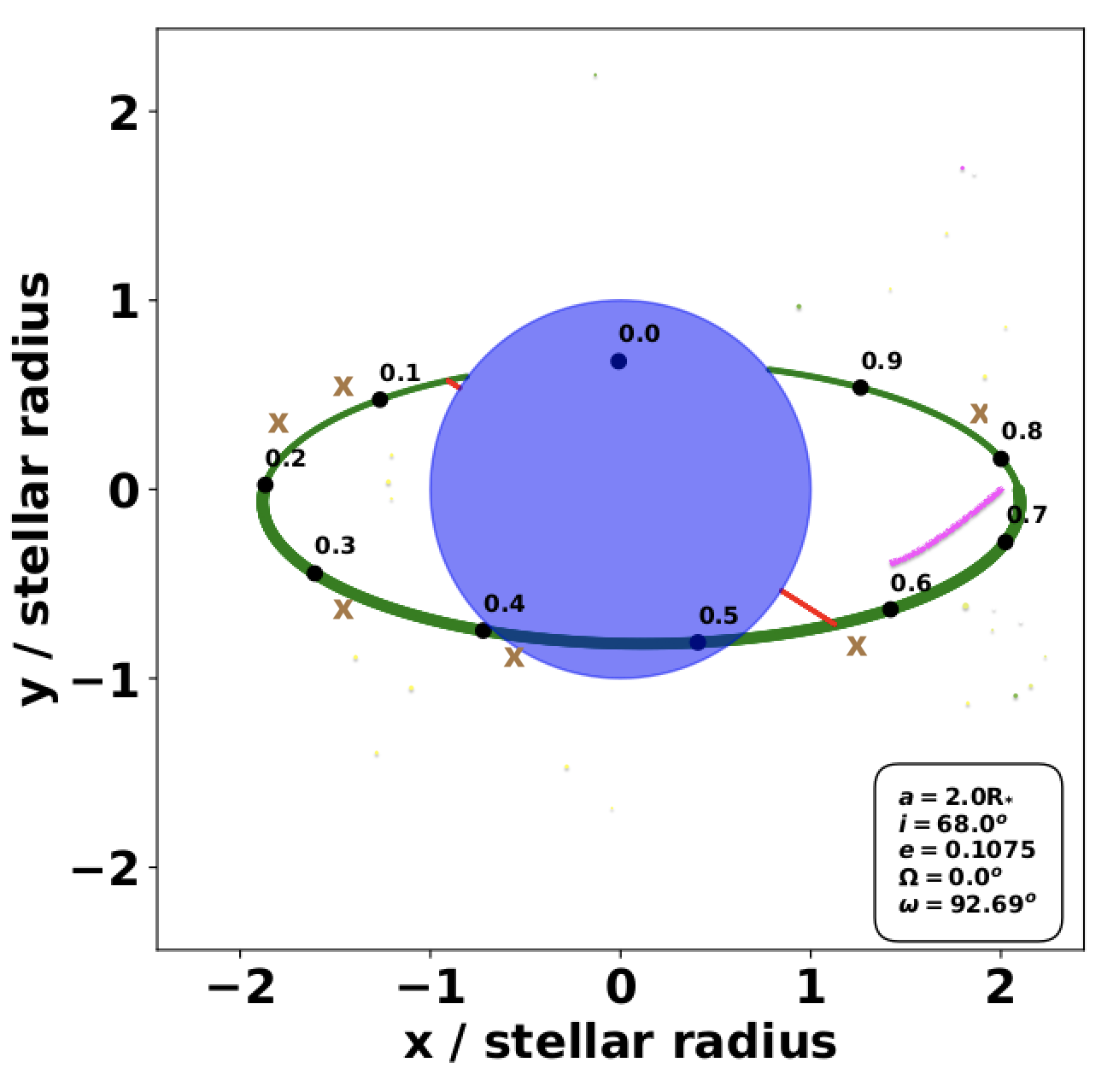
Figure 1: Orbit of the neutron star (solid green line) around its massive stellar companion (in blue) as seen from Earth. The values of orbital separation (a), the orbital inclination (i), eccentricity (e), longitude of periastron ($\Omega$), and periastron angle ($\omega$) are given in the lower right panel (Jenke et al., 2012). Black dots along the orbit mark orbital phases while the red solid line is the main axis of the orbit. The phases for NuSTAR (magenta line) and NICER observations (brown ‘X’ marks) are plotted.

OAO 1657–415 was observed with NuSTAR (Harrison et al. 2013) in June 2019 during the orbital phase of 0.612-0.743, where phase 0 is the mid-eclipse time (MJD 52674.1199) and P_orb = 10.447355 d (Falanga et al., 2015) that we use to determine orbital phase throughout the paper. NuSTAR consists of two focal plane modules, FPMA and FPMB, each made of four pixelated detectors (DET0-DET3) spanning an energy range of 3–79  keV. We used nupipeline version 0.4.6 to generate cleaned event files, which also provides the recommended source and background regions. These region files were an input to nuproducts that we used for extracting data products like light curves and spectrum.

We fit the FPMA and FPMB spectra simultaneously (keeping the relative instrument normalization free) using HEASOFT 6.26.1 and CALDB version 20201217 with XSPEC 12.10.1f. The spectra were binned using an optimal binning scheme adapted from Kaastra & Bleeker (2016). We performed timing analysis in the barycenter-corrected frame and corrected the NuSTAR light curves for orbital motion and subtracted the background. Using the epoch folding technique, we determined the pulse period, which was used to create the energy resolved pulse profiles of OAO 1657$-$415 and to obtain the pulse phase resolved spectra (details in Section 3).

2.2 NICER

The NICER observations of OAO 1657–415, although not simultaneous with the NuSTAR observations, are very useful for studying the variation of absorption with orbital phase. We monitored OAO 1657–415 with NICER during April-May 2020 (ObsID: 364901090) for three orbital cycles of the binary (see Table 1). For NICER data reduction, screening has been applied to all NICER data using the calibration release xti20200722 as follows: Data from detectors 14, 34, and 54 were excised, as these detectors have exhibited intermittent problems being prone to excess electronic noise (e.g., Riley et al. 2019). Good time intervals are defined using continuous intervals with no packet loss, in which the ISS was outside the South Atlantic Anomaly and pointing aligned within 1.5 arcmin to the target, with all subsystems configured nominally. We require SUN_ANGLE $>$ 60 degrees (or when in shadow, SUNSHINE==0), with ELV $>$ 20 and BR_EARTH $>$ 30. In addition, the remaining 49 active detectors were screened based on X-ray overshoot, and undershoot rates which serve as indicators of liveness, particle background, and optical loading, respectively. Any detector outside the median by ¿ 15 median absolute deviation (MAD) (roughly, an unbiased equivalent of $\approx$ 10$\sigma$) is rejected. Calibration ARF and RMF files were generated, respectively, by summing or averaging the per$-$FPM products. In selecting good events, the default fast-to-slow ratio (‘trumpet’) filter was employed, and the background spectra were derived using the standard ‘3C50’ background model (Remillard et al., 2022).

For the same filtering criteria as described above, the NICER light curves were extracted from the event files obtained from nicerl2 to which barycentric corrections were performed with barycorr using latest ephemeris file JPLEPH.430. We then searched for pulsations in each ObsIDs using efsearch and generated pulse profiles using efold.

3 Results

3.1 NuSTAR results

The NuSTAR analysis thread recommend fitting the FPMA and FPMB spectra separately while keeping their relative instrument normalization free. The spectra for OAO 1657–415 are shown in Fig. 2. Since the spectra above 70 keV are background dominated, we fit the 3–70 keV NuSTAR spectra with phenomenological XSPEC (Arnaud, 1996) continuum models viz., CUTOFFPL, HIGHECUT (White et al., 1983) and NEWHCUT (Burderi et al., 2000).

$$\mathrm{CUTOFFPL}(E)=A\ E^{-\Gamma}\times{\rm e}^{-(E)/E_{\rm{fold}}}\\$$ (1)

$$\mathrm{HIGHECUT}(E)=A\ E^{-\Gamma}\times\ \begin{cases}1&(E\leq E_{\rm{cut}})\\ {\rm e}^{-(E-E_{\rm{cut}})/E_{\rm{fold}}}&(E>E_{\rm{cut}})\\ \end{cases}$$ (2)

$$\mathrm{NEWHCUT}(E)=\begin{cases}\ E^{-\Gamma}&E\leq E_{\rm{cut}}-W/2\\ AE^{3}+BE^{2}+CE+D,&E_{\rm{cut}}-W/2\leq E\leq E_{\rm{cut}}+W/2\\ E^{-\Gamma}\times\ {\rm e}^{(E_{\rm{cut}}-E)/E_{\rm{fold}}},&E\geq E_{\rm{cut}}+W/2\\ \end{cases}$$ (3)

While the fits were comparable using these models (i.e., similar ${\chi_{r}^{2}}$ per degrees of freedom; d.o.f), the MCMC corner plots indicated that CUTOFFPL permits the least degeneracy among the spectral parameters. Therefore, the best continuum to describe the source spectrum corresponds to an absorbed power law with an exponential cutoff and a Gaussian function to model the K_α emission line leading to ${\chi_{r}^{2}}$/d.o.f. as 1.72/666. With this model, we still see some wavy residuals (especially below 5 keV) and in order to smoothen it, we added a partial covering model to account for local absorption which improved the ${\chi_{r}^{2}}$/d.o.f. to 1.24/665 d.o.f. This inclusion of two absorption components is motivated by the fact that absorption column density in HMXBs (N_H) comprise two components: global absorption, NH₁, that arise from a component that is extended, possibly the stellar wind, large-scale structures like an accretion wake (El Mellah & Casse, 2015), Co-rotating Interaction Regions (CIRs, Nazé et al., 2013; Massa et al., 2014), and the interstellar column density (Wilms et al., 2000). The second component is for local absorption NH₂ very close to the neutron star that blocks the compact source partially (with partial covering fraction f) in size or partially in time (clumps/structures).

With the addition of a partial covering model, the value of absorption column density, NH₁ could not be constrained. We therefore froze this to the Galactic line of sight absorption of 1.8 $\times$ 10²² atoms cm^-2 and the free component, NH₂, encompasses a time average of the local absorption, which is not fully covering due to moving structures/clumps. The latter component of the partial covering model is well known to be a crucial component necessary to fit the X-ray spectrum of OAO 1657–415 (Audley et al., 2006; Pradhan et al., 2014; Jaisawal & Naik, 2014; Jaisawal et al., 2021; Pradhan et al., 2019b).

Note that, in addition to the K_α line, since the X-ray spectrum of OAO 1657–415  exhibits complex iron line features viz. Fe XXVI (6.97 keV) and Fe XXV (6.7 keV) and K_β (7.1 keV), we also tried to account for these lines by freezing the line energy and width of these lines detected with Chandra/HETG (Pradhan et al., 2019b) while allowing the normalization to vary. However, even with this exercise, we were not able to constrain the normalization of these lines – possibly due to the limited spectral resolution of NuSTAR - nor was there any improvement in the spectral fitting. The NuSTAR spectrum therefore only allowed constraining the Gaussian parameters for the Fe K_α line in the source. We list the complete parameters for spectral fitting in Table 2 and the time-averaged spectrum is shown in Fig. 2. The MCMC corner plot for the average spectrum is shown in Fig. A.1.

X-ray variability of HMXBs can be studied using a few different techniques. For instance, the tracks exhibited by wind-accretion HMXBs on color-color diagram during absorption can be explained by partial covering model with variable absorption (Hirsch et al., 2019; Grinberg et al., 2020). Another technique is to investigate the X-ray variability through hardness-ratio (hard/soft) resolved spectral analysis: since soft X-ray photons are more easily absorbed than higher energy photons, the X-ray variability caused by absorption is reflected in the hardness-ratio (hard/soft) resolved spectral analysis (see, e.g., Grinberg et al. 2017; Pradhan et al. 2019a).

In this paper, we have performed hardness-ratio (HR; 10-70 keV/3-10 keV) resolved spectral and timing analysis: we determined the time segments where the hardness ratio changed significantly by using the Bayesian Blocks analysis (Scargle et al., 2013). Such a technique has also been previously used in the case of supergiant fast X-ray transients, SFXTs by Sidoli et al. (2019) to identify intervals of significant intensity variability in the light curves of a sample of these objects observed by XMM-Newton. The block fitness function used is the one for point measurements and the ncp_prior was chosen to have a false alarm rate around 1% using Fig. 6 of Scargle et al. (2013). We verified that the number of spurious changes of the HR was compatible with expectations by running a sample of 50 simulations with constant count rate, drawn from a distribution with noise equivalent to the measured light curve of each source. We obtained 21 time intervals with this technique where the HR is revealed to undergo significant variations. When we fit the HR resolved spectra from these 21 segments for the two FPMs, we find that one of the segments showed a possible degeneracy in the spectral parameters and therefore to mitigate any statistical limitation, we merged this segment with the next immediate one. As a result, we therefore divided the whole observation in 20 segments and the fits to these HR-resolved segments (shown in Fig. 3) were performed using C-statistics and the confidence intervals were determined using MCMC chains.

In Fig. 3, we show the NuSTAR light curves (counts per second), hardness-ratio (HR) with 20 time segments delimited by red vertical solid lines, local absorption column density NH₂ (in units of 10²² cm^-2), covering fraction f, equivalent width (EW in keV), normalization or Fe K$\alpha$ line (Fe_norm in photons cm^-2 s^-1), spectral index $\Gamma$, folding energy E_fold (in keV), normalization of spectral index ($\Gamma_{\rm{norm}}$ in photons keV^-1 cm^-2 s^-1 at 1 keV) and absorbed flux in 3–70 keV (in units of 1$\times~{}10^{-9}$ erg cm^-2 s^-1). From the plot we make the following observations (i) The HR and NH₂ to follow a similar variability trend, (ii) The NH₂ and EW of Fe line are correlated, (iii) The covering fraction always remains high, ranging between 90-100%. The corner plots corresponding to some segments in Fig. 3, where the absorption values are medium, low, and high (1, 7, 19) in these fits are shown in Figures A.2, A.3 and A.4.

We extracted the pulse profiles for each of these 20 time segments (Fig. 4) and investigated the pulse profile morphology with time. For pulse profile analysis, we performed the orbital correction (using orbital parameters from Falanga et al. 2015) and we use efsearch to determine the pulse period of the pulsar to be 37.01072 s ($\pm$ 0.00034) at MJD 58645.

The pulse profiles are created from the orbital and barycenter corrected light curve with the above period and an epoch of MJD 58645.0000857 so that the minimum of the first peak i.e., the peak more prominent at high energies, is approximately at pulse phase zero. Our choice coincides with the phase zero in Sharma et al. (2022) and can be used to compare the results obtained from many other satellites since it is a very recognizable feature in the pulse profile of OAO 1657–415. Note that for clarity, we show pulse profiles twice over the same spin phase.

The same pulse profiles evolution with time and absorption are shown in Fig. 4 and Fig. 5 respectively. From these two figures, we can see no significant evolution of the pulse profiles with either time or absorption.

Furthermore, in order to investigate the variability of pulse profiles with energy, we also extracted the pulse profiles for various energy ranges shown. In some HMXBs, the energy dependence of pulse profiles is not prominent (e.g., Pradhan et al. 2015). Thanks to the large area of NuSTAR, we were able to identify a dip near spin phase 0.15 for the first time in OAO 1657–415. We show the energy-resolved pulse profiles on the left of Fig. 6 and the ratio to the right, to find that (i) the dip at spin phase 0.15 seems to be evolving with energy and increase from 5-30 keV and vanishes thereafter, and (ii) dips at spin phases 0, 0.4 and 0.6 become less prominent with increasing X-ray energy.

Finally, we performed spin-phase resolved spectral analysis in 16 phase bins using the same model as determined by the average spectrum. The average pulse profile is plotted on the top of Fig. LABEL:spec-phase and the absorption on the second panel from the top. The absorption increases during dips in the pulse profiles, except during the dip around 0.15 where there is a decrease in local absorption NH₂ and changes in the folding energy, E_fold. We see a variation of the Fe K$\alpha$ normalization (Fe_norm; in photons cm^-2 s^-1) with spin phase. The covering fraction $\rm{f}$ does not change much with phase, and the normalization of the power law ($\Gamma_{\rm{norm}}$; in photons keV^-1 cm^-2 s^-1 at 1 keV) scales with X-ray normalized intensity for each segment. The Pearson coefficient between the count rate (proxy for normalized intensity) and $\Gamma_{\rm{norm}}$ for the 16 segments is $\sim$ 0.92. All these spectral variations remain valid following the inspection of corner plots as well. For reference, we show corner plots in Figures A.5, A.6, and A.7 of three-phase intervals where the absorbing column density is low, high, and medium.

3.2 NICER results

We fit the 1-10 keV spectra from individual observations of NICER with a partial covering absorbed power law for global and local absorption (i.e., NH₁ and NH₂) along with a Gaussian for the iron K$\alpha$ line. One ObsID, 3649010801, showed hints of highly ionized lines at 6.97 keV and 6.7 keV two more Gaussian were used to fit these lines. The individual spectral plots are shown in Fig. 8 and the variation of spectral parameters with time and phase are shown in Fig. 9.

The NICER monitoring of OAO 1657–415 over its three different orbital cycles of the source (spectra in Fig. 8) reveals large variations in the absorption column density with orbital phase, (see Fig. 9). We find that the pulsations are present in at least 4 of the 6 ObsIDs (NICER pulse profiles in Fig. LABEL:nicer-pp).

The four ObsIDs 3649010101, 3649010401, 3649010501, 3649010901 were folded at epochs MJD 58961.0003005, 58967.0000643, 58969.0002214, 58977.0 with the periods of 37.096000 s, 37.064932 s, 37.084932 s, 37.055759 s respectively obtained from the NICER lightcurves. The choice of these epochs approximately coincided the minimum of the first peak of the pulse profile to be at pulse phase zero.

Although the dip at phase 0.15 seen in NuSTAR is not visible, the dip at 0.4 as seen in NuSTAR  (this work) and Suzaku observations (Pradhan et al., 2014) is clearly visible.

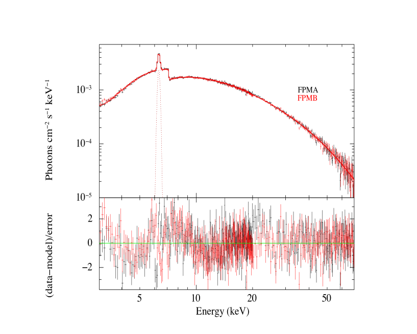
Figure 2: Time-averaged spectrum of OAO 1657–415 for NuSTAR FPMA (black), FPMB (red) modelled with CUTOFFPL for orbital phase 0.612–0.743. The corner plot for spectral parameters for the time averaged spectrum is given in Fig. A.1.

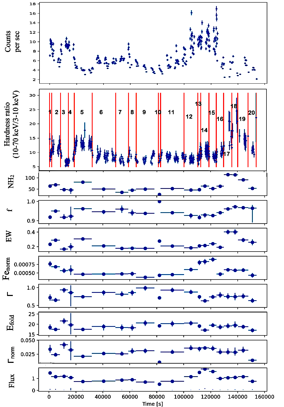
Figure 3: From top to bottom are the NuSTAR light curves (counts per second), Hardness-ratio (HR) with 20 time segments delimited by red vertical solid lines, absorption column density N_H2 (in units of 10²² cm^-2), covering fraction f, equivalent width (EW in keV), normalization or Fe K$\alpha$ line Fe_norm (in photons cm^-2 s^-1), spectral index $\Gamma$, folding energy E_fold (in keV), normalization of the power law $\Gamma_{\rm{norm}}$ (in photons keV^-1 cm^-2 s^-1 at 1 keV) and absorbed flux in 3–70 keV (in 1$\times~{}10^{-9}$ erg cm^-2 s^-1). N_H1 is frozen at the line of sight absorption of $1.8\times 10^{22}$ atoms cm^-2. Note that not all parameters could be constrained in segment 10 and therefore no errors are plotted for this segment. The corner plots corresponding to some segments where the absorption values are medium, low, and high (1, 7, 19) in these fits are shown in Figures A.2, A.3 and A.4.

Figure 4: Pulse profiles over each time segment of constant hardness ratio (see panel in Fig. 3). Time segments are indicated in the upper right corner. The Y-axis is the normalized counts/sec with respect to the average for each plot.

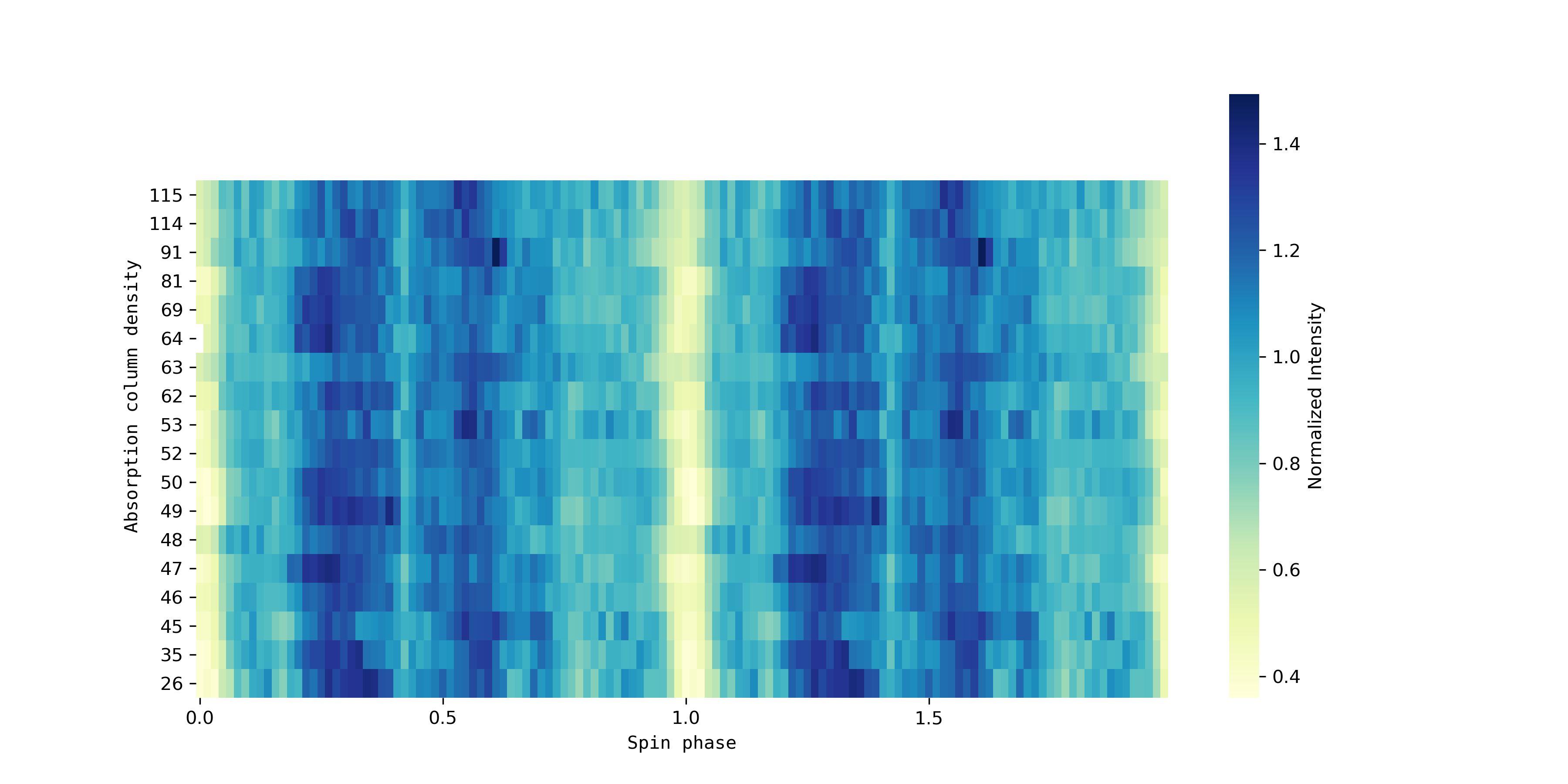
Figure 5: Pulse profiles of OAO 1657–415 for HR-resolved segments in order of increasing absorption column density (units of 10²² cm^-2) marked along the Y-axis from down upwards and spin phase along the X-axis. The color maps represent the pulse normalized intensity.

Figure 6: Left: Energy-resolved pulse profiles for FPMA+B light curves where a dip at $\sim$ 0.15 is clearly seen. Right: Ratio of pulse profiles with energy denoted inside the panel.

Figure 8: NICER spectra of OAO 1657–415 at different orbital phases, with ObsID and relevant orbital phases noted inside the figures.

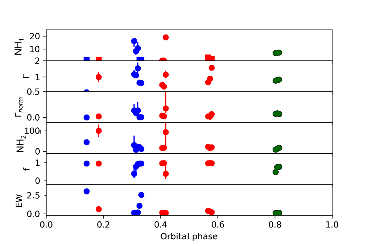
Figure 9: Results of NICER monitoring of OAO 1657–415 over three different orbits of OAO 1657–415 shown by three colors. From top to bottom are global absorption column density (NH₁; in units of 10²² cm^-2), spectral index $\Gamma$, normalization of spectral index ($\Gamma_{\rm norm}$; in photons/keV/cm²/s at 1 keV), local absorption column density (NH₂; in units of 10²² cm^-2), and equivalent width of iron line (EW; in keV). The square symbols in the uppermost plot indicate the values of NH₁ where the errors could not be determined and were frozen to its best-fit values.

Table 2: Results of the spectral fit in the energy range 3.0-70.0 keV with the CUTOFFPL model. All errors are quoted for 90% confidence level. We froze the value of NH₁ to the line of sight absorption of 1.8 $\times$ 10²² cm^-2. From left to right, the local absorbing column density NH₂, covering fraction f, spectral index $\Gamma$, normalization of the power law ($\Gamma_{\rm{norm}}$; units of photons/keV/cm²/s at 1 keV), folding energy, E_fold followed by energy, width, equivalent width of iron line and the reduced chi-square per degrees of freedom.

$N_{\textrm{H2}}$	f	$\Gamma$	$\Gamma_{\rm{norm}}$	$E_{\textrm{fold}}$	$E_{\textrm{Fe}}$	$\sigma_{\textrm{Fe}}$	EW	${\chi_{r}^{2}}$/d.o.f
(1022 cm-2)	(Covering fraction)			(keV)	(keV)	(keV)	equivalent width (keV)
53 $\pm$ 2	0.93 $\pm$ 0.01	0.70 $\pm$ 0.04	0.020 $\pm$ 0.001	18 $\pm$ 0.5	6.31 $\pm$ 0.01	0.11 $\pm$ 0.02	0.26 $\pm$ 0.01	1.24/665

4 Discussion

4.1 X-ray variability in OAO 1657–415 caused by clumpy winds

The light curve of OAO 1657$-$415 as measured by NuSTAR display changes in count rate in few ks interval seen in many classical SGXBs (Walter et al., 2015; Pradhan et al., 2014). The good statistics of NuSTAR data allowed us to perform a detailed investigation of the changes in the HR as a function of time. In order to better understand the origin of these variations, we first identified 20 time intervals corresponding to the most noticeable HR changes and then used these intervals to perform an HR resolved spectral analysis of the NuSTAR data with the same model used for the average spectrum.

In Fig. 3, it can be appreciated that the rises in the HR (e.g., intervals 2, 5, 17, 18, 19) are largely related to the increases in the local absorption column density (above the baseline value of $\sim$ 50$\times$10²² cm^-2) and increase in the equivalent width of the iron line. At intervals 3-4, 7-8, 12, there is a drop of the absorption below the average value of $\sim$ 50$\times$10²² cm^-2 along with a drop in the HR below its average value of $\sim$ 10. For intervals 17, 18 and 19, there is a dramatic increase in absorption as well as HR. These large variations in absorption column density do not translate into modifications in the photon index and folding energy. It is agreement with previous conclusions in the literature (Pradhan et al., 2014; Jaisawal & Naik, 2014) and leads us to favor the possibility that it is caused by a clumpy stellar wind rather than a varying continuum hardness. Our findings are consistent with the physical scenario in which the soft X-ray photons are intercepted by cold matter (neutral Fe) in the clumpy wind, resulting in an increase in the absorption column density and equivalent width of the Fe line.

During the segments (i.e., 17-19), there is also a decrease of the X-ray count rate compared to its preceding segments (i.e., 13-16). Such behavior where absorption increase during X-ray flux decays has been previously observed in other classical SgXBs like IGR J18027-2016 (Pradhan et al., 2019a) as well as in most Supergiant Fast X-ray Transients (Bozzo et al., 2016, 2017). The proposed interpretation is also related to the clumpiness of the stellar wind. The increase in the absorption close to the rise of the X-ray flux can be an indication that the event is being triggered by a dense clump partly intercepting the orbit of the compact object along the line of sight to the observer. When the accretion of the clump material begins, the X-ray flux increases and causes a partial photoionization of the clump surrounding the neutron star. This leads to a rapid decrease of the absorption, which returns to values measured before the flux only when the X-ray fluxes decrease along the decay of the flare (the value of absorption after the flare depends also on the location of the re-arranging of the accreted clump with respect to the line of sight to the observer). Such an interpretation has been proposed for OAO 1657–415 earlier in the literature, which we discuss as follows. During the Suzaku observation spanning orbital phase of 0.1-0.3, the absorption varied in the range $\sim$ 10-100 $\times$ 10²² cm^-2 and the correspondingly measured equivalent width of Fe K$\alpha$ line was $\sim$ 0.1-1.0  keV (Pradhan et al., 2014). During an Chandra observation carried out in phase 0.5-0.6, the absorption was $\sim$ 70 $\times$ 10²² cm^-2 and the corresponding equivalent width was $\sim$ 1 keV (Pradhan et al., 2019b). In the current observation, although the average equivalent width is lower than previous observations, we find that the equivalent width of the iron line scales with the absorption as expected. Such a variation is fully consistent with fluorescence emission of X-rays in the clumps of matter around the neutron star (e.g., Fig. 1 of Pradhan et al. 2018). Calculating the 3-70 keV flux in each HR segment and assuming a distance of 7.1 kpc for the source (Audley et al., 2006), we find that the X-ray luminosity varies from L_X $\sim$ 4–10 $\times$ 10³⁶ erg s${-1}$ through the NuSTAR observation.

Following the results of pulse phase resolved spectroscopy of NuSTAR data (Fig. LABEL:spec-phase), we argue that the dip in pulse profiles at phase 0.4 corresponds to an increase in NH₂ and is therefore possibly caused by obscuration of X-rays. On the other hand, the dip at phase 0.15 could have a different explanation (see section 4.2 for details on this observation). From the spin phase resolved spectroscopy, we also find that the iron line also showed a flux variation with pulse phase, indicating anisotropic matter distribution around the neutron star as expected from clumpy winds. Additionally, from NICER observations, we note a correlation between absorption and equivalent width of iron line, which is also consistent with what is seen from earlier measurements in the literature. This scenario is agreeable with reprocessing of X-ray photons in the cold fluorescence matter, possibly clumps in the wind. We will revisit this discussion in sections 4.3 and 4.5 below.

4.2 Dip at spin phase 0.15: Changes in viewing geometry or a transient accretion disk?

We report, for the first time, a dip at spin phase of $\sim$ 0.15 seen in the NuSTAR pulse profiles. The dip in OAO 1657–415 lasts for roughly 0.06 of the spin phase (i.e., $\sim$ 2 s) and, albeit variable in different time segments (see, Fig. 4), is visible throughout the NuSTAR observation of $\sim$ 150 ks. The strength of the dip is energy-dependent, being the most prominent between 5-30 keV (see, Fig. 6), the same energy range in which the X-ray photons undergo inverse Compton scattering and produce the high energy cut-off in the X-ray spectrum of HMXBs. Although the occurrence of dips in pulse profiles are not unusual when the X-rays are intercepted by clumps in the stellar wind, such dips caused by obfuscation in clumps are short-lived and are often accompanied by a large increase in absorption (e.g., dip at phase 0.4 in Fig. LABEL:spec-phase). From the spin phase resolved spectroscopy, we see that there is no increase in absorption around phase 0.15, but rather this dip is accompanied by a change in folding energy at the same phase (see, Fig. LABEL:spec-phase). These findings, coupled with the fact that the dip last throughout the entire NuSTAR observation of $\sim$ 150 ks exposure, the likely explanation is that the dip at 0.15 is caused by a change in viewing geometry — possibly X-ray emission in multiple accretion columns or spectral changes due to the formation of a transient disk.

Note that in earlier analysis of the same NuSTAR data (Saavedra et al. 2022; Sharma et al. 2022), the period at which the light curves are folded are determined from individual time segments. In our case, we have performed the orbital correction followed by determining the spin period from the whole data set, which is then used to fold the light curves. The advantage of the latter approach (versus search over smaller time segments) is that the spin period is determined with greater accuracy. This will therefore allow us to study the evolution of pulse profile morphology over the duration of the observation more accurately. We also confirmed the spin period derived here in this work, after correcting for the orbital motion, is consistent with the Fermi/GBM measurement interpolated to the time of this observation.

This dip in OAO 1657–415 is also reminiscent of the dip discovered in the XMM-Newton observations of the Be X-ray binary, EXO 2030+375 during the Type-I outburst caused by self-obscuration of the accretion stream passing through the observer line of sight (Ferrigno et al., 2016). While a similar possibility of an accretion stream passing the observer line of sight in OAO 1657–415 cannot be ruled out, given that the dip is energy dependent and most prominent in the critical energy range of 5-30 keV in which the photons undergo inverse Comptonization to produce a cut-off in the X-ray spectrum, the former possibility of spectral changes due to X-ray emission in multiple accretion columns or the formation of a transient accretion disk are more likely as argued earlier.

We also discovered from the Fermi/GBM monitoring that during the time of the NuSTAR observation the pulsar was spinning down for $\sim$ 300 days after a long spin-up of $\sim$ 800 days. Since OAO 1657–415 is presumed to host a transient accretion disk, we cannot exclude the possibility that the spin up followed by the spin down of the pulsar (as seen from GBM monitoring) could be related to changes in the emitting region caused by a transient accretion disk. The signatures of a transient accretion disk are manifested as changes in the X-ray spectrum and the pulse profiles has earlier been seen for GX 301-2 with NuSTAR (Nabizadeh et al., 2019). Additionally, the very low terminal wind speed in OAO 1657–415 strongly favors the formation of wind-captured disks due to the significant shearing of the flow (Shapiro & Lightman, 1976). In El Mellah et al. (2019), the authors argue that transient disks are likely to form when the stellar wind speed at the orbital separation is of the order of or lower than the orbital speed, which is the case in OAO 1657–415. Taani et al. (2019) also singled out OAO 1657–415 as a HMXB susceptible to host a wind-captured disk, given its orbital and wind parameters. A better understanding of accretion-induced torques is required to understand whether the torque reversal captured by GBM could have been provoked by a transient wind-captured disk.

As argued earlier, while absorption of soft X-rays in clumps could cause dips in the pulse profiles, in such cases, one would also expect the pulse profiles to change with hardness ratio, the same is not seen here (see Fig 4, Fig 5). This is probably due to the fact that the NuSTAR band pass is dominated by hard X-rays, where absorption has lesser energy dependence. We refer the readers to Fig. 2 of Hirsch et al. (2019) for the effect of absorption on the soft X-ray spectral shape where a partial covering remove flux at soft energies making only the direct component visible.

Earlier results have revealed that the lack of pulsations (pulse fraction less than 2%) in the soft X-ray emission of OAO 1657–415 across the Chandra observation (Pradhan et al., 2019b) and during the time interval of the Suzaku observation with the highest absorption ($\sim$ 10²⁴ cm^-2 in interval ‘C’; Pradhan et al. 2014) can be ascribed to the effect of dense clumps obscuring the X-ray source. Compared to these data, the NuSTAR observation shows a much lower averaged absorption ($\sim$ 5$\times$10²³ cm^-2) and it is indeed possible that during the NuSTAR observation the neutron star was passing through a less dense region of the stellar wind, as expected for any reasonable assumption of the properties of the wind of the O supergiant (see e.g., Martínez-Núñez et al. 2017 and references therein). The low density of the accretion environment during the NuSTAR observation explains the fact that in none of the 20 HR resolved time intervals, we observed a disappearance of pulsations (see Fig. 4 for pulse profiles of the segments). On the other hand, the NICER observations reveal that pulsations were detected in 4 of the 6 ObsIDs. The two ObsIDs (3649010301 and 3649010801) are highly absorbed ($\sim$ 10²⁴ cm^-2) and no pulsations were detected during these observations.

Note that a relatively recent class of sources, named the ultraluminous X-ray pulsars (ULXPs), exhibit strong variability in the pulsed fractions. Such pulse dropout phenomena have been observed in some ULX pulsars: M82 X-2 (Bachetti et al., 2014), NGC 7793 P13 (Fürst et al., 2016; Israel et al., 2017a), NGC 5907 ULX-1 (Israel et al., 2017b), and NGC 300 ULX1 (Carpano et al., 2018). While the most plausible explanation for such a behavior has been proposed to be the onset of the propeller effect (Tsygankov et al., 2016), the exact mechanism for pulse dropout is still not established. Interestingly, such pulse dropouts uncorrelated with flux have been reported for some HMXBs as well: Vela X-1 (Kretschmar et al., 2000), LMC X-4 (Brumback et al., 2018), SMC X-1 (Pike et al., 2019; Pradhan et al., 2020) and OAO 1657–415 (Jaisawal et al., 2021). For all the four sources, the pulse-dropout is unlikely to be caused by the onset of the propeller regime, since the cessation of pulsations were not caused by cessation of accretion/X-ray flux variations. Note also that the pulse dropouts in all these three sources occur in hard X-rays and are therefore unlikely to be caused by increased absorption in an intervening matter (e.g., clumps).

4.3 Where are the Iron lines formed in OAO 1657–415?

Given the high inclination of the source, the compact object in OAO 1657–415 undergoes eclipses for $\sim$ 20% of the orbital period. Using ASCA observations, Audley et al. (2006) made the first estimate for Fe K$\alpha$ line-forming region as 19 ($\pm$ 12) lt-sec from the compact object. This value was based on the intensity variations of Fe K$\alpha$ line in and out of eclipse. Similar results were also obtained under the assumption that clumps are composed of neutral hydrogen in a moderately ionized surrounding (Jaisawal & Naik, 2014), limited by ionization parameter (Kallman & McCray, 1982) below.

$$\xi=\frac{L_{X}}{nR^{2}}\leqslant 10^{2}{\rm~{}in~{}erg~{}cm/s}$$ (4)

where $L_{X}$ is the X-ray luminosity of the source, $n$ is the free electron density in the clump at a distance $R$ from the compact object. It should however be noted that the luminosity of the source is variable and for the Chandra observation at orbital phase of $\sim$ 0.55, where the luminosity was two orders of magnitude less than the Suzaku observation, the limiting inner radius of the Fe K$\alpha$ line-forming region was found to be much closer to the neutron star at $\sim$ 2.5 lt-sec (Pradhan et al., 2019b). Note however that the Chandra observation was carried out in a ‘special’ phase where long-term INTEGRAL light curves show a dip when the compact object is completely enshrouded by dense (and large, possibly phase-locked) matter (Barnstedt et al., 2008; Pradhan et al., 2019b).

Using our current measurements, we now try to constrain the regions of neutral and ionized iron line formation in OAO 1657–415. Assuming that the inter-clump medium is void, the volume filling factor $f_{vol}$ can be used to determine the number density $n$ from $n=n_{\rm wind}/f_{\rm vol}$ (Sundqvist et al., 2018), where $n_{\rm wind}$ is the stellar wind density at the orbital separation if the wind were smooth and isotropic, given by:

$$n_{\rm wind}=\frac{\dot{M}/m_{\rm p}}{4\pi a^{2}v_{a}},$$ (5)

where $\dot{M}$ is the mass-loss rate, $m_{\rm p}$ is the mass of the proton, $a$ is the orbital separation, and $v_{a}$ is the wind velocity at a distance $a$ from the donor star. Working along the line joining the star to the neutron star, we can rewrite Eqn. (4):

$$\xi=\xi_{0}\left(\frac{R}{{a-R}}\right)^{2},$$ (6)

where:

$$\xi_{0}=4\pi f_{\rm vol}\frac{m_{p}v_{a}L_{X}}{\dot{M}}.$$ (7)

We look for the distance $R=R_{100}$ to the neutron star where $\xi=100$ erg cm$/$s using Eqn. (6). We take a terminal wind speed of 250 km s^-1, a stellar radius of 25R_⊙ and a mass loss rate of 1$\times 10^{-6}$ M_⊙ yr^-1 (Mason et al., 2012). We find that $R_{100}$ ranges from 20 to 40 lt-s for nominal volume filling factors, f_vol = 0.1-0.3 (Sundqvist et al., 2018), and for L_X = 4-10 $\times$ 10³⁶ erg s${-1}$. The luminosity is calculated from the 3-70 keV fluxes in HR segments for a distance of 7.1 kpc (Audley et al., 2006). This value of line-forming region of K$\alpha$ line is consistent with the value obtained by Audley et al. (2006). However, it is to be understood as a lower limit since we worked along the line joining the two bodies but at the orbital phase of the current NuSTAR observation (0.612-0.743), it does not correspond to the line-of-sight. If the geometry matches the classic one considered by Hatchett & McCray (1977), the latter intercepts the $\xi=100$ erg cm$/$s surface at a distance from the neutron star larger than $R_{100}$.

Among the NICER observations (see, Fig. 8), one ObsID 3649010801 showed hints of ionized lines, and we fit this spectrum to obtain the ratio of the 6.97 to the 6.7 keV line $\sim$ 3. This translates to $\xi\geq 10^{3.8}$ (refer to Figure 8 of Ebisawa et al. 1996). Thereafter, using Eqn. 4, the line emitting region $R$ for these ionized lines for $n$ $\sim$ 3$\times$$10^{13}$ cm^-3 is $\sim$ 7$\times$10⁸  cm ($\sim$ 0.02 lt-s). The ionized lines form much closer to the compact object than the neutral Fe K$\alpha$ lines.

4.4 Non-detection of a CRSF line

We found that the phase-averaged NuSTAR spectrum of OAO 1657–415 can be described by a relatively hard power-law continuum modified by an exponential cutoff plus a partial covering component and fluorescence iron K$\alpha$ line at 6.4 keV. There is no evidence for the previously reported CRSF at 36 keV (see Section 1 for details on previous works). We looked for Gaussian like absorption lines in the phase-averaged NuSTAR spectrum between 10 keV and 50 keV with width of 0.1 times the energy bin and find an upper limit on the optical depth of is about 0.06 (at 90% confidence level). This value is far smaller than the typical value that is encountered in all other sources with confirmed CRSF (Maitra, 2017; Staubert et al., 2019; Pradhan et al., 2021).

Using the same NuSTAR data, Saavedra et al. (2022) claimed the detection of a CRSF at $\sim$35 keV with a width of $\sim$29 keV in the averaged spectrum of the source. The authors however do not make use of a partial covering absorption component as a part of their continuum model, which give rise to wavy structures in the residuals, interpreted as a cyclotron line. We additionally tested the above scenario by fitting the spectrum of OAO 1657–415  with the continuum parameters frozen to the values reported in Saavedra et al. (2022). We notice an extremely broad and shallow feature extending from 20 keV up to the highest energy range used for the spectral fit. We are unable to constrain the width of this feature (line centroid fits at $\sim$56 keV) and this typically represents an inadequacy in the spectral model or incorrect continuum modelling. While Sharma et al. (2022) were able to model a CRSF varying in the range $\sim$ 38–42 keV with a width $\sim$ 0.8–5 keV in some time segments, there were no discussions regarding the statistical significance of the feature in the paper except the improvement in $\chi^{2}$ for the spectral fit by adding the multiplicative model ‘gabs’ or ‘cyclabs’. This is not adequate to test the presence of the cyclotron line (see Orlandini et al., 1999) and needs to be treated with caution. Note that based on the spin phase-resolved spectroscopy, we see a dip-like feature around spin phase 0.2 at 40 keV which was reminiscent of the CRSF line, but it is not seen in other phase intervals and is possibly spurious since the F-test reveals the probability of chance improvement (PCI) $\sim$ 0.75. Therefore, in the event of the claimed cyclotron line being model-dependent, the absorption like residuals seen in the X-ray spectrum is likely a result of imperfect continuum modelling - possibly a result of steepening of the spectrum above 20 keV as discussed in Orlandini et al. (1999) - and not a true CRSF.

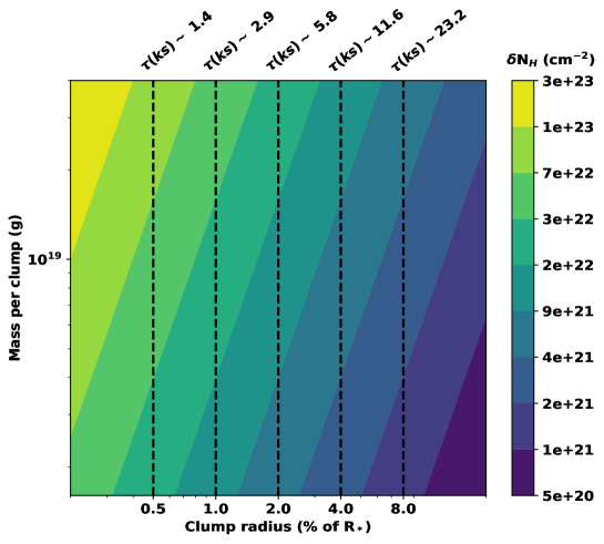
Figure 11: Coherence time scale $\tau$ scale of column density time series is represented in ks at the top and the color map shows the standard deviation $\delta N_{H}$ for different clump sizes and masses. The values of orbital separation, the orbital inclination, eccentricity, longitude of periastron, and periastron angle are taken from Jenke et al. (2012) and the orbital phase of the pulsar is 0.25.

4.5 Clump size estimates in OAO 1657–415: caveats and future outlook

While X-ray variability is attributed to clumpy stellar winds, there are a still a lot of open questions. For instance, although line driven instability can in principle generate important density variations in the stellar wind of massive stars (see e.g., Sundqvist et al. 2018), the details and geometry are not yet fully understood. Furthermore, even if the wind is highly inhomogeneous, it is unclear whether the flow will be smoothed as it is accreted and clumps mix or whether additional instabilities will fragment the flow and make it more inhomogeneous. For instance, when the wind crosses the hydrodynamic bow shock surrounding the neutron star at a distance of the order of the accretion radius, the clumps mix in the shocked region (El Mellah et al., 2018a). It results in a smoother flow and a lower time variability than in the ballistic framework where clumps are instantaneously captured when their impact parameter is lower than the accretion radius (Ducci et al., 2009; Oskinova et al., 2012). On the other hand, magneto-centrifugal gating mechanisms at the outer rim of the neutron star magnetosphere could produce additional time variability (Bozzo et al., 2008).

In the literature, there are discrepancies up to a factor of 10 on the clump sizes and of a factor of 1,000 on the clump masses (see Pradhan et al., 2014; El Mellah et al., 2018b). At this point, hardness ratio-resolved X-ray spectroscopy is useful to constrain micro-structure of the wind like the density of individual clumps, the number of clumps per unit volume and the radius of clumps in HMXBs (in’t Zand, 2005; Pradhan et al., 2014, 2019a).

Recently, El Mellah et al. (2020) designed a model to characterize variable column density due to unaccreted foreground clumps intercepting the line-of-sight. The framework is built upon the first model drawn by Grinberg et al. (2015). It assumes that spherical clumps are launched from the photosphere of the donor star. The clumps expand as they flow away from the star on radial trajectories and follow a pre-defined beta velocity profile (Puls et al., 2008). The inter-clump environment is empty, the number of clumps is realistic and set by the stellar mass loss rate, the individual clump mass, the size of the system and the wind speed. They found that the statistical properties of the N_H time series could be linked to the properties of the clumps. At each orbital phase, the characteristic time scale of absorption variability and the standard deviation with respect to the median column density profile depend on the size and on the mass of the individual clumps (see El Mellah et al., 2020, for more detail). It is especially dependent on the properties of the clumps along the line of sight which are the closest from the donor star.

Taking advantage of the fact that OAO 1657$-$415 has been observed with numerous X-ray facilities like Suzaku (Pradhan et al., 2014), Chandra (Pradhan et al., 2019b), NICER and NuSTAR (this work) at various orbital phases, we attempt to constrain the clump sizes based on El Mellah et al. (2020). We computed the predicted coherence times ($\tau$; time duration during which there is smooth variation in absorption column density) and standard deviation of the column density, $\delta N_{H}$, for different clump masses and sizes of OAO 1657–415 using the orbital parameters derived by Falanga et al. (2015).

We first neglect the micro-structure of the wind and assume that it is smooth in order to derive the global parameters (i.e. the ones not linked to the clump properties). These parameters have been shown by El Mellah et al. (2020) to be the orbital inclination $i$, the ratio of the orbital separation $a$ to stellar radii $R_{\star}$ and the beta exponent $\beta$ (assuming a negligible eccentricity). In addition, the normalization of the profile, $N_{H,0}$, is given by:

$$N_{H,0}=\frac{\dot{M}_{\star}}{R_{\star}v_{\infty}}$$ (8)

where $\dot{M}_{\star}$ is the stellar mass loss rate and $v_{\infty}$ is the terminal wind speed. The best models we could obtain by qualitatively similar absorption profiles agree with the orbital parameters commonly derived in the literature: $i\sim$65–70 degrees and $a\sim 2R_{\star}$ (Falanga et al., 2015; Mason et al., 2012). Furthermore, the models favor a $\beta$ exponent around 2, suggestive of a progressive wind acceleration. The column density scales we find are of the order of 10²⁴cm^-2, coherent with a terminal wind speed of 250 km s^-1, a stellar radius of 25R_⊙ and a mass loss rate of 1$\times 10^{-6}$ M_⊙ yr^-1, though the latter is somewhat higher than the upper limit reported by Falanga et al. (2015). We could then constrain the clump size and mass based on Figure 10 in El Mellah et al. (2020) but for parameters suited for OAO 1657–415. In Figure 11, the coherence time scale $\tau$ is represented in kiloseconds at the top while the color map shows the standard deviation $\delta N_{H}$ for different clump sizes and masses for orbital phase 0.25. This exercise illustrates a novel methodology to measure more accurately different clump sizes and masses in HMXBs.

The above method is particularly important since the fundamental prerequisite to characterize clumps in stellar wind is to have the ability to makes measurements in absorption at timescales of the order of or smaller than the coherence timescale. However, the limitation set by the detector properties (area, cadence of observations) hinders the study of time-resolved spectroscopy down to the required short time scales and therefore the clump size estimates determined this way should be regarded as upper limits. Therefore, for example, from Suzaku measurements, we could measure the absorption changes in timescales of only $\sim$ 10 ks (Fig. 9 of Pradhan et al. 2014), the relatively small collecting area of the Suzaku/XIS do not permit time-resolved spectroscopy at shorter time scales. The fast spectral changes associated with the source can be most effectively studied with XMM-Newton due to its ability to observe the source uninterruptedly, thanks to the orbit of the satellite. The other two operating X-ray spacecrafts with largest areas at the present are NuSTAR and NICER, the results of which are presented here. While both are indispensable in investigating the X-ray properties of the pulsar as we see above, both have limitations caused by cadence of observation. The low altitude and low inclination orbit of NuSTAR are inter dispersed with gaps in data thereby limiting the required cadence necessary for this kind of work (see section 6.2 of El Mellah et al. 2020 for details). On the other hand, while NICER has been very efficient in orbital monitoring of the source spread across days, the cadence of one observation can be less than 90 min long over which the spacecraft orbits Earth.

Short-term variability studies of X-ray binaries on smaller time scales have been made in the literature using indirect methods such color-color diagrams (Nowak et al., 2011; Grinberg et al., 2020). In the near future, high throughput X-ray missions such as XRISM (XRISM Science Team, 2020), eXTP (in’t Zand et al., 2019), and Athena (Nandra et al., 2013) can enable short-term absorption variability studies, even for moderately faint sources. With Athena, for example, high S/N spectra of HMXBs are possible in timescales of few hundred seconds (Lomaeva et al., 2020; Amato et al., 2021). Therefore, efforts like the current paper - dedicated to the study of short term variability of absorption and their implications - are now necessary to act as segues for these upcoming high-resolution missions and their role in studying the inhomogeneity of stellar winds.

5 Summary

In this paper we exploited the NuSTAR and NICER observations of OAO 1657–415 in order to carry out for the first time a detailed HR-resolved spectral analysis of the X-ray emission from OAO 1657–415. Taking advantage of the good energy resolution and large effective area of NuSTAR, the HR-resolved spectral analysis could be carried out in all cases on few ks timescales and thus be used to characterize the clumpy winds and locate where emission lines are formed in OAO 1657–415. Additionally, data from both instruments helped us characterize the pulse profiles in OAO 1657–415. We summarize the main findings of our work below.

• The HR and spin phase resolved spectroscopic studies of OAO 1657–415 with NuSTAR and the spectral variation obtained by monitoring the source with NICER are consistent with the presence of clumpy stellar winds in the system.

• We report for the first time a dip around 0.15 in the pulse profiles from NuSTAR, possibly caused by changes in viewing geometry. Probable explanations include X-ray emission in multiple accretion columns or spectral changes due to the formation of a transient disk.

• The neutral iron lines are formed far away from the neutron star - possibly in the clumps in the stellar wind while the ionized lines are formed closer to the neutron star and probably within the magnetosphere.

• The NuSTAR spectrum clearly revealed that the putative CRSF at $\sim$ 36 keV is not a real feature and the dip reported in the literature is possibly caused by turnover of the X-ray spectrum at $\sim$ 20  keV (Orlandini et al., 1999).

• We did not detect pulsations in 2 of the 6 NICER observations. This is possibly due to increased absorption of X-ray photons in the surrounding matter.

• We illustrate a novel methodology by El Mellah et al. (2020) to measure clump sizes and masses in HMXBs more accurately based on absorption measurements and orbital parameters of the source. Finally, we segue our current work into the future of X-ray binaries with upcoming X-ray missions.

Appendix A Corner plots

The appendix contains corner plots for the average spectrum and three hardness-ratio resolved and three pulse phase resolved segments where the absorption column density are low, medium and high.

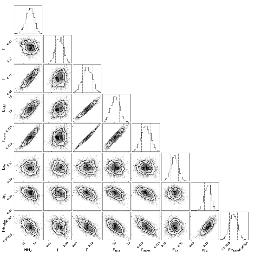
Figure A.1: Corner plots for the average spectrum.

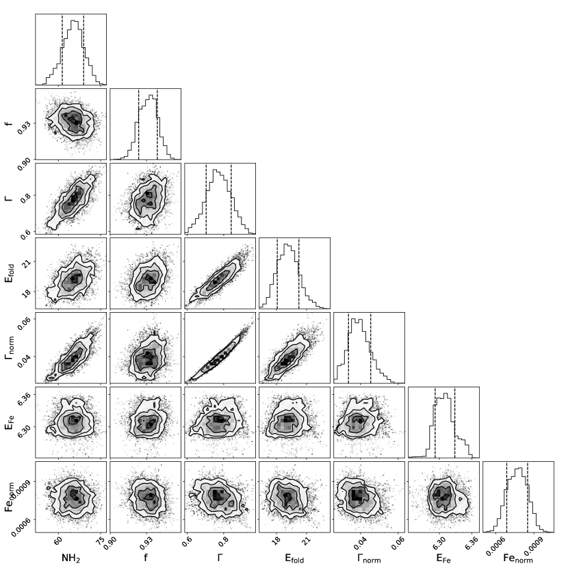
Figure A.2: Corner plots for hardness-ratio resolved segment 1.

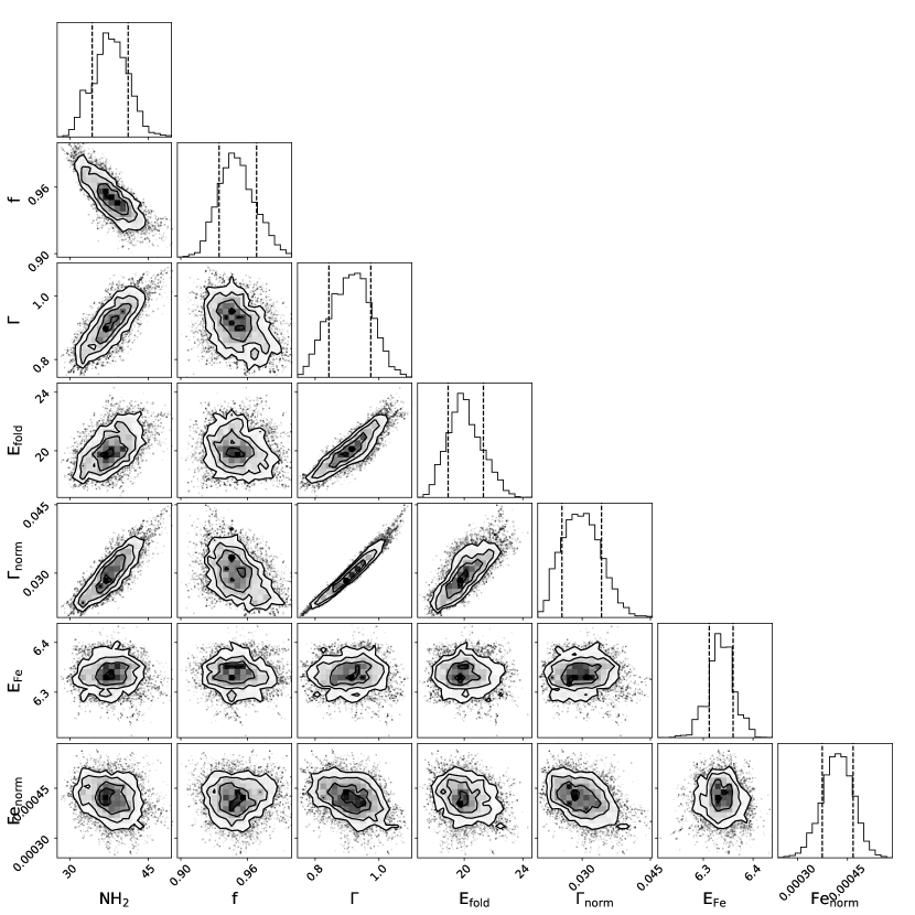
Figure A.3: Corner plots for hardness-ratio resolved segment 7.

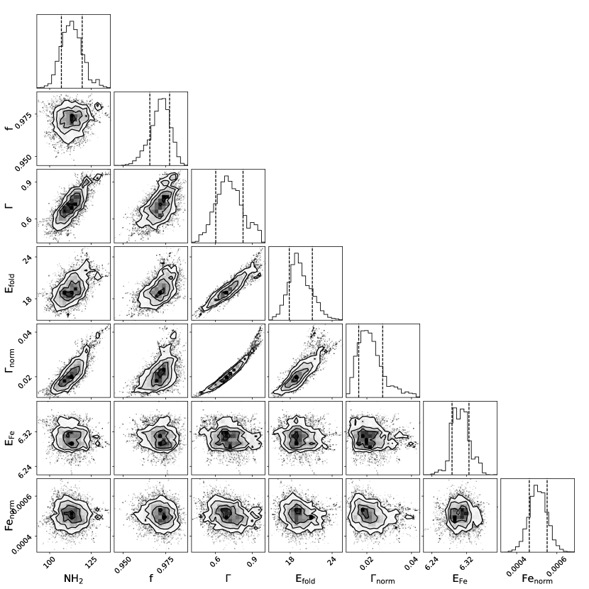
Figure A.4: Corner plots for hardness-ratio resolved segment 19.

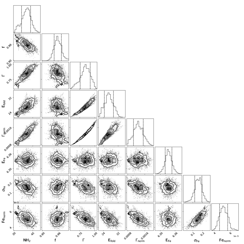
Figure A.5: Corner plots for third phase bin (phase $\sim$ 0.2) in Fig. LABEL:spec-phase.

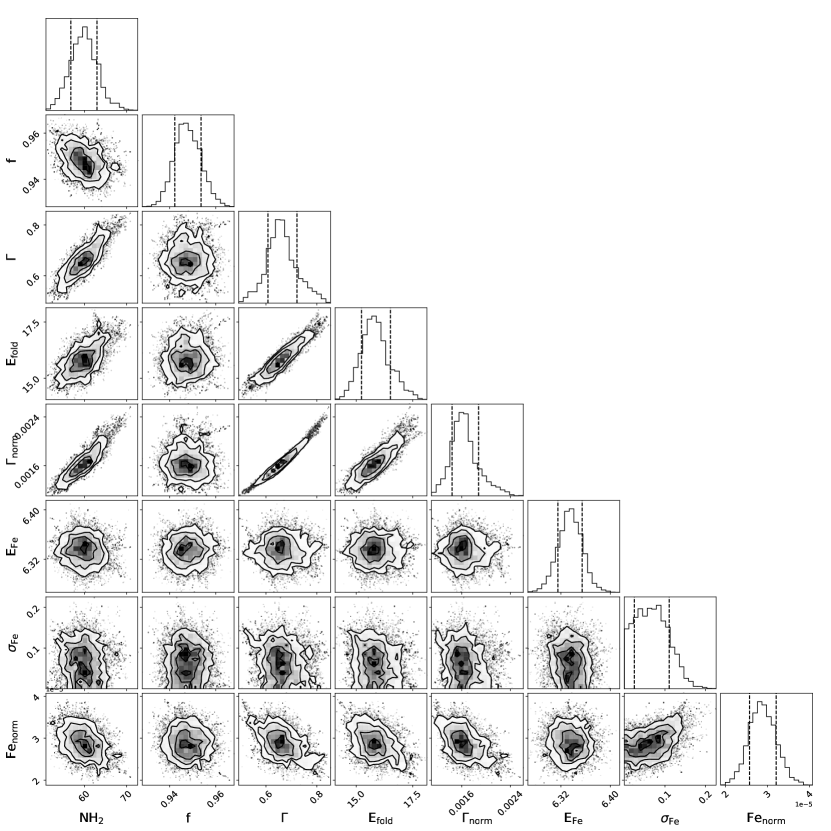
Figure A.6: Corner plots for seventh phase bin (phase $\sim$ 0.4) in Fig. LABEL:spec-phase.

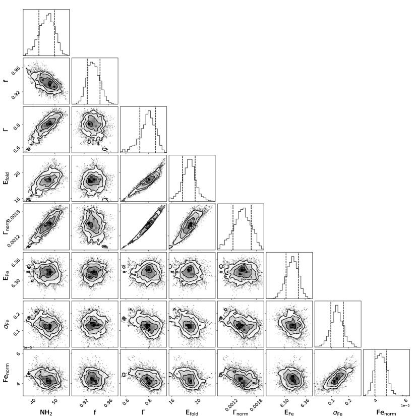
Figure A.7: Corner plots for thirteenth phase bin (phase $\sim$ 0.8) in Fig. LABEL:spec-phase.

References

- Amato et al. (2021) Amato, R., Grinberg, V., Hell, N., et al. 2021, A&A, 648, A105, doi: 10.1051/0004-6361/202039125
- Arnaud (1996) Arnaud, K. A. 1996, in Astronomical Society of the Pacific Conference Series, Vol. 101, Astronomical Data Analysis Software and Systems V, ed. G. H. Jacoby & J. Barnes, 17
- Audley et al. (2006) Audley, M. D., Nagase, F., Mitsuda, K., Angelini, L., & Kelley, R. L. 2006, MNRAS, 367, 1147, doi: 10.1111/j.1365-2966.2006.10003.x
- Bachetti et al. (2014) Bachetti, M., Harrison, F. A., Walton, D. J., et al. 2014, Nature, 514, 202, doi: 10.1038/nature13791
- Barnstedt et al. (2008) Barnstedt, J., Staubert, R., Santangelo, A., et al. 2008, A&A, 486, 293, doi: 10.1051/0004-6361:20078707
- Baykal (1997) Baykal, A. 1997, A&A, 319, 515
- Becker & Wolff (2007) Becker, P. A., & Wolff, M. T. 2007, ApJ, 654, 435
- Bozzo et al. (2017) Bozzo, E., Bernardini, F., Ferrigno, C., et al. 2017, A&A, 608, A128, doi: 10.1051/0004-6361/201730398
- Bozzo et al. (2008) Bozzo, E., Falanga, M., & Stella, L. 2008, ApJ, 683, 1031, doi: 10.1086/589990
- Bozzo et al. (2022) Bozzo, E., Ferrigno, C., Oskinova, L., & Ducci, L. 2022, MNRAS, 510, 4645, doi: 10.1093/mnras/stab3688
- Bozzo et al. (2016) Bozzo, E., Bhalerao, V., Pradhan, P., et al. 2016, A&A, 596, A16, doi: 10.1051/0004-6361/201629311
- Brumback et al. (2018) Brumback, M. C., Hickox, R. C., Bachetti, M., et al. 2018, The Astrophysical Journal, 861, L7, doi: 10.3847/2041-8213/aacd13
- Burderi et al. (2000) Burderi, L., Di Salvo, T., Robba, N. R., La Barbera, A., & Guainazzi, M. 2000, ApJ, 530, 429, doi: 10.1086/308336
- Caiazzo & Heyl (2021) Caiazzo, I., & Heyl, J. 2021, MNRAS, 501, 109, doi: 10.1093/mnras/staa3428
- Carpano et al. (2018) Carpano, S., Haberl, F., Maitra, C., & Vasilopoulos, G. 2018, MNRAS, 476, L45, doi: 10.1093/mnrasl/sly030
- Chakrabarty et al. (1993) Chakrabarty, D., Grunsfeld, J. M., Prince, T. A., et al. 1993, ApJ, 403, L33, doi: 10.1086/186715
- Corbet (1986) Corbet, R. H. D. 1986, MNRAS, 220, 1047
- Driessen et al. (2021) Driessen, F. A., Kee, N. D., & Sundqvist, J. O. 2021, A&A, 656, A131
- Driessen et al. (2022) Driessen, F. A., Sundqvist, J. O., & Dagore, A. 2022, A&A, 663, A40
- Ducci et al. (2009) Ducci, L., Sidoli, L., Mereghetti, S., Paizis, A., & Romano, P. 2009, MNRAS, 398, 2152
- Ebisawa et al. (1996) Ebisawa, K., Day, C. S. R., Kallman, T. R., et al. 1996, Publications of the Astronomical Society of Japan, 48, 425, doi: 10.1093/pasj/48.3.425
- El Mellah & Casse (2015) El Mellah, I., & Casse, F. 2015, MNRAS, 454, 2657, doi: 10.1093/mnras/stv2184
- El Mellah et al. (2020) El Mellah, I., Grinberg, V., Sundqvist, J. O., Driessen, F. A., & Leutenegger, M. A. 2020, A&A, 643, A9, doi: 10.1051/0004-6361/202038791
- El Mellah et al. (2019) El Mellah, I., Sander, A. A. C., Sundqvist, J. O., & Keppens, R. 2019, A&A, 622, A189, doi: 10.1051/0004-6361/201834498
- El Mellah et al. (2018a) El Mellah, I., Sundqvist, J. O., & Keppens, R. 2018a, MNRAS, 475, 3240
- El Mellah et al. (2018b) —. 2018b, MNRAS, 475, 3240. https://arxiv.org/abs/1711.08709
- Ertan (2017) Ertan, Ü. 2017, MNRAS, 466, 175, doi: 10.1093/mnras/stw3131
- Falanga et al. (2015) Falanga, M., Bozzo, E., Lutovinov, A., et al. 2015, A&A, 577, A130, doi: 10.1051/0004-6361/201425191
- Ferrigno et al. (2016) Ferrigno, C., Pjanka, P., Bozzo, E., et al. 2016, A&A, 593, A105, doi: 10.1051/0004-6361/201527837
- Fürst et al. (2016) Fürst, F., Walton, D. J., Harrison, F. A., et al. 2016, ApJ, 831, L14, doi: 10.3847/2041-8205/831/2/L14
- Gendreau et al. (2016) Gendreau, K. C., Arzoumanian, Z., Adkins, P. W., et al. 2016, in Society of Photo-Optical Instrumentation Engineers (SPIE) Conference Series, Vol. 9905, Space Telescopes and Instrumentation 2016: Ultraviolet to Gamma Ray, ed. J.-W. A. den Herder, T. Takahashi, & M. Bautz, 99051H, doi: 10.1117/12.2231304
- Grinberg et al. (2020) Grinberg, V., Nowak, M. A., & Hell, N. 2020, A&A, 643, A109, doi: 10.1051/0004-6361/202039183
- Grinberg et al. (2015) Grinberg, V., Leutenegger, M. A., Hell, N., et al. 2015, A&A, 576, A117, doi: 10.1051/0004-6361/201425418
- Grinberg et al. (2017) Grinberg, V., Hell, N., El Mellah, I., et al. 2017, A&A, 608, A143, doi: 10.1051/0004-6361/201731843
- Harrison et al. (2013) Harrison, F. A., Craig, W. W., Christensen, F. E., et al. 2013, ApJ, 770, 103, doi: 10.1088/0004-637X/770/2/103
- Hatchett & McCray (1977) Hatchett, S., & McCray, R. 1977, ApJ, 211, 552, doi: 10.1086/154962
- Hirsch et al. (2019) Hirsch, M., Hell, N., Grinberg, V., et al. 2019, A&A, 626, A64, doi: 10.1051/0004-6361/201935074
- in’t Zand (2005) in’t Zand, J. J. M. 2005, A&A, 441, L1
- in’t Zand et al. (2019) in’t Zand, J. J. M., Bozzo, E., Qu, J., et al. 2019, Science China Physics, Mechanics, and Astronomy, 62, 29506, doi: 10.1007/s11433-017-9186-1
- Israel et al. (2017a) Israel, G. L., Belfiore, A., Stella, L., et al. 2017a, Science, 355, 817, doi: 10.1126/science.aai8635
- Israel et al. (2017b) Israel, G. L., Papitto, A., Esposito, P., et al. 2017b, MNRAS, 466, L48, doi: 10.1093/mnrasl/slw218
- Jaisawal & Naik (2014) Jaisawal, G. K., & Naik, S. 2014, Bulletin of the Astronomical Society of India, 42, 147. https://arxiv.org/abs/1601.02345
- Jaisawal et al. (2021) Jaisawal, G. K., Naik, S., Epili, P. R., et al. 2021, Journal of Astrophysics and Astronomy, 42, 72, doi: 10.1007/s12036-021-09701-x
- Jenke et al. (2012) Jenke, P. A., Finger, M. H., Wilson-Hodge, C. A., & Camero-Arranz, A. 2012, ApJ, 759, 124, doi: 10.1088/0004-637X/759/2/124
- Kaastra & Bleeker (2016) Kaastra, J. S., & Bleeker, J. A. M. 2016, A&A, 587, A151, doi: 10.1051/0004-6361/201527395
- Kallman et al. (2015) Kallman, T., Dorodnitsyn, A., & Blondin, J. 2015, ApJ, 815, 53, doi: 10.1088/0004-637X/815/1/53
- Kallman & McCray (1982) Kallman, T. R., & McCray, R. 1982, ApJS, 50, 263, doi: 10.1086/190828
- Kretschmar et al. (2000) Kretschmar, P., Kreykenbohm, I., Wilms, J., et al. 2000, in American Institute of Physics Conference Series, Vol. 510, The Fifth Compton Symposium, ed. M. L. McConnell & J. M. Ryan, 163–167, doi: 10.1063/1.1303195
- Lomaeva et al. (2020) Lomaeva, M., Grinberg, V., Guainazzi, M., et al. 2020, A&A, 641, A144, doi: 10.1051/0004-6361/202037807
- Maitra (2017) Maitra, C. 2017, Journal of Astrophysics and Astronomy, 38, 50, doi: 10.1007/s12036-017-9476-3
- Martínez-Núñez et al. (2017) Martínez-Núñez, S., Kretschmar, P., Bozzo, E., et al. 2017, Space Sci. Rev., doi: 10.1007/s11214-017-0340-1
- Mason et al. (2012) Mason, A. B., Clark, J. S., Norton, A. J., et al. 2012, MNRAS, 422, 199, doi: 10.1111/j.1365-2966.2012.20596.x
- Mason et al (2009) Mason et al, A. B. 2009, A&A, 505, 281. https://arxiv.org/abs/0907.3876
- Massa et al. (2014) Massa, D., Oskinova, L., Fullerton, A. W., et al. 2014, MNRAS, 441, 2173, doi: 10.1093/mnras/stu565
- Nabizadeh et al. (2019) Nabizadeh, A., Mönkkönen, J., Tsygankov, S. S., et al. 2019, A&A, 629, A101, doi: 10.1051/0004-6361/201936045
- Nandra et al. (2013) Nandra, K., Barret, D., Barcons, X., et al. 2013, arXiv e-prints, arXiv:1306.2307. https://arxiv.org/abs/1306.2307
- Nazé et al. (2013) Nazé, Y., Oskinova, L. M., & Gosset, E. 2013, ApJ, 763, 143, doi: 10.1088/0004-637X/763/2/143
- Nowak et al. (2011) Nowak, M. A., Hanke, M., Trowbridge, S. N., et al. 2011, ApJ, 728, 13, doi: 10.1088/0004-637X/728/1/13
- Orlandini et al. (1999) Orlandini et al., M. 1999, A&A, 349, L9
- Oskinova et al. (2012) Oskinova, L. M., Feldmeier, A., & Kretschmar, P. 2012, MNRAS, 421, 2820
- Pike et al. (2019) Pike, S. N., Harrison, F. A., Bachetti, M., et al. 2019, ApJ, 875, 144, doi: 10.3847/1538-4357/ab0f2b
- Pradhan et al. (2018) Pradhan, P., Bozzo, E., & Paul, B. 2018, A&A, 610, A50, doi: 10.1051/0004-6361/201731487
- Pradhan et al. (2019a) Pradhan, P., Bozzo, E., Paul, B., Manousakis, A., & Ferrigno, C. 2019a, ApJ, 883, 116, doi: 10.3847/1538-4357/ab3a40
- Pradhan et al. (2020) Pradhan, P., Maitra, C., & Paul, B. 2020, ApJ, 895, 10, doi: 10.3847/1538-4357/ab8224
- Pradhan et al. (2014) Pradhan, P., Maitra, C., Paul, B., Islam, N., & Paul, B. C. 2014, MNRAS, 442, 2691, doi: 10.1093/mnras/stu1034
- Pradhan et al. (2013) Pradhan, P., Maitra, C., Paul, B., & Paul, B. C. 2013, MNRAS, 436, 945, doi: 10.1093/mnras/stt1504
- Pradhan et al. (2021) Pradhan, P., Paul, B., Bozzo, E., Maitra, C., & Paul, B. C. 2021, Monthly Notices of the Royal Astronomical Society, 502, 1163, doi: 10.1093/mnras/stab024
- Pradhan et al. (2015) Pradhan, P., Paul, B., Paul, B. C., Bozzo, E., & Belloni, T. M. 2015, MNRAS, 454, 4467, doi: 10.1093/mnras/stv2276
- Pradhan et al. (2019b) Pradhan, P., Raman, G., & Paul, B. 2019b, MNRAS, 483, 5687, doi: 10.1093/mnras/sty3441
- Puls et al. (2008) Puls, J., Vink, J. S., & Najarro, F. 2008, A&A Rev., 16, 209, doi: 10.1007/s00159-008-0015-8
- Remillard et al. (2022) Remillard, R. A., Loewenstein, M., Steiner, J. F., et al. 2022, AJ, 163, 130, doi: 10.3847/1538-3881/ac4ae6
- Riley et al. (2019) Riley, T. E., Watts, A. L., Bogdanov, S., et al. 2019, ApJ, 887, L21, doi: 10.3847/2041-8213/ab481c
- Saavedra et al. (2022) Saavedra, E. A., Fogantini, F. A., Combi, J. A., García, F., & Chaty, S. 2022, A&A, 659, A48, doi: 10.1051/0004-6361/202142066
- Scargle et al. (2013) Scargle, J. D., Norris, J. P., Jackson, B., & Chiang, J. 2013, ApJ, 764, 167, doi: 10.1088/0004-637X/764/2/167
- Shapiro & Lightman (1976) Shapiro, S. L., & Lightman, A. P. 1976, ApJ, 204, 555, doi: 10.1086/154203
- Sharma et al. (2022) Sharma, P., Sharma, R., Jain, C., & Dutta, A. 2022, MNRAS, 509, 5747, doi: 10.1093/mnras/stab3436
- Sidoli et al. (2019) Sidoli, L., Postnov, K. A., Belfiore, A., et al. 2019, MNRAS, 487, 420, doi: 10.1093/mnras/stz1283
- Sokolova-Lapa et al. (2021) Sokolova-Lapa, E., Gornostaev, M., Wilms, J., et al. 2021, A&A, 651, A12, doi: 10.1051/0004-6361/202040228
- Staubert et al. (2019) Staubert, R., Trümper, J., Kendziorra, E., et al. 2019, A&A, 622, A61, doi: 10.1051/0004-6361/201834479
- Sundqvist et al. (2018) Sundqvist, J. O., Owocki, S. P., & Puls, J. 2018, A&A, 611, A17, doi: 10.1051/0004-6361/201731718
- Taani et al. (2019) Taani, A., Karino, S., Song, L., et al. 2019, Research in Astronomy and Astrophysics, 19, 012, doi: 10.1088/1674-4527/19/1/12
- Tsygankov et al. (2016) Tsygankov, S. S., Mushtukov, A. A., Suleimanov, V. F., & Poutanen, J. 2016, MNRAS, 457, 1101, doi: 10.1093/mnras/stw046
- Walter et al. (2015) Walter, R., Lutovinov, A. A., Bozzo, E., & Tsygankov, S. S. 2015, A&A Rev., 23, 2, doi: 10.1007/s00159-015-0082-6
- West et al. (2020) West, B., Becker, P., & Wolfram, K. 2020, in American Astronomical Society Meeting Abstracts, American Astronomical Society Meeting Abstracts, 408.06
- White & Pravdo (1979) White, N. E., & Pravdo, S. H. 1979, ApJ, 233, L121, doi: 10.1086/183089
- White et al. (1983) White, N. E., Swank, J. H., & Holt, S. S. 1983, ApJ, 270, 711, doi: 10.1086/161162
- Wilms et al. (2000) Wilms, J., Allen, A., & McCray, R. 2000, ApJ, 542, 914, doi: 10.1086/317016
- XRISM Science Team (2020) XRISM Science Team. 2020, arXiv e-prints, arXiv:2003.04962. https://arxiv.org/abs/2003.04962