Quench dynamics of the Schwinger model via variational quantum algorithms

Abstract

We investigate the real-time dynamics of the $(1+1)$-dimensional U(1) gauge theory known as the Schwinger model via variational quantum algorithms. Specifically, we simulate quench dynamics in the presence of an external electric field. First, we use a variational quantum eigensolver to obtain the ground state of the system in the absence of an external field. With this as the initial state, we perform real-time evolution under an external field via a fixed-depth, parameterized circuit whose parameters are updated using McLachlan’s variational principle. We use the same Ansatz for initial state preparation and time evolution, by which we are able to reduce the overall circuit depth. We test our method with a classical simulator and confirm that the results agree well with exact diagonalization.

I Introduction

Lattice gauge theory is a powerful tool for studying quantum field theory. In the conventional approach, simulations are performed using the Monte-Carlo method, which requires the exponential of the action $\exp({\rm i}S)$ to be positive and real. This protocol suffers from a sign problem when we consider e.g. a topological term, a finite chemical potential, and real-time dynamics.

Instead of Monte Carlo, one can use the Hamiltonian formalism, which avoids the sign problem as it is not a sampling-based approach. However, the quantum state grows exponentially with the size of the system, making this approach not feasible on classical computers. The advantage of quantum computers is that the computational resources can be kept logarithmic in system size, as was shown in the seminal paper by Jordan, Lee, and Preskill [1]. Since that work, digital quantum simulation in the context of quantum field theory has been attracting a lot of interest [2, 3, 4, 5, 6, 7, 8, 9, 10, 11, 12, 13, 14, 15, 16, 17, 18, 19, 20, 21, 22, 23, 24, 25, 26, 27, 28, 29, 30, 31, 32, 33, 34, 35, 36, 37, 38, 39, 40, 41, 42, 43, 44, 45, 46, 47, 48, 49, 50, 51, 52, 53, 54, 55, 56, 57, 58, 59, 60, 61, 62, 63]. In particular, real-time simulation is one of the important applications since it can in general not be captured efficiently by any known classical method. The standard simulation method on quantum computers uses Suzuki-Trotter decomposition, where the circuit depth increases as the evolution time does, which causes a decoherence problem on noisy intermediate-scale quantum (NISQ) devices. Efficient algorithms have been proposed for the preparation of the ground state of certain classes of quantum systems, such as Quantum Imaginary Time evolution and a Quantum Lanczos algorithm [64]. Variational algorithms combine quantum computations with classical optimizations, and are able to perform both state preparation and time evolution using an approach called variational quantum simulation (VQS), even if the accuracy of the method depends on the chosen variational Ansatz. A VQS method based on Mclachlan’s variational principle (MVP) was proposed in [65, 66] in which the evolved states are approximated by parameterized states (Ansatz) with a fixed depth.

In this work, we apply this variational method to investigate the real-time dynamics of $(1+1)$ dimensional U(1) gauge theory called the Schwinger model. Specifically, we perform real-time simulation after turning on an external electric field to see electron-positron pair creations induced by the external field, which is the so-called Schwinger mechanism [86]. This is similar to what was considered in [87] where a classical tensor network approach was used . See Fig. 1 for the sketch of our simulation protocol.

Figure 1: Sketch of our simulation. We start from the ground state in the absence of external electric field $q$. We then suddenly turn on the external field $q$ and evolve the state via the Hamiltonian with $q>0$. These states are approximated by the same Ansatz $\ket{\psi(\lambda)}$.

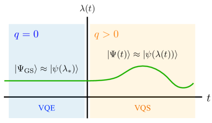
We first prepare the ground state $\ket{\Psi_{\text{GS}}}$ in the absence of the external electric field $q$ by using a variational quantum eigensolver (VQE). At initial time $t=0$ the external field is then suddenly turned on (the quantum quench), and the time evolution in the system with an external electric field is then studied. We approximate the dynamical states $\ket{\Psi(t)}=e^{-{\rm i}H_{q\neq 0}t}\ket{\Psi_{\text{GS}}}$ by the same Ansatz used in VQE, and evolve the parameters according to MVP. Note that by performing both state preparation and time evolution through variational circuits, the depth of a quantum circuit is greatly reduced.

The structure of this paper is organized as follows. Section II introduces the Hamiltonian of the Schwinger model and observables we will focus on. Section III explains a method we will use for the simulation. In Section IV results are presented and compared them with exact diagonalization. Finally, conclusions are given in Section V.

II The Schwinger model

The Schwinger model describes quantum electromagnetism in one spatial and one time dimension. This model is relatively simple, and can in fact be solved analytically [89, 90] in the massless limit. It is nevertheless a very interesting field theory to study, since despite its simplicity it shares several features with the QCD, the theory of the strong interaction, such as confinement and charge screening [91, 92].

II.1 Lattice Hamiltonian and spin description

Here we will define the lattice Hamiltonian and introduce its spin description. We mostly follow the convention used in [10]. First of all, the Lagrangian of the continuum Schwinger model is given by

$$\mathcal{L}_{\rm con} =-\frac{1}{4}F_{\mu\nu}F^{\mu\nu}+{\rm i}\bar{\psi}\gamma^{\mu}(\partial_{\mu}+{\rm i}gA_{\mu}-m)\psi$$

$$\qquad+\frac{g\theta}{4\pi}\epsilon_{\mu\nu}F^{\mu\nu}\,.$$ (1)

Here the first two terms correspond to the kinetic term of the gauge boson and fermion, respectively, while the third term denotes a topological term that does not affect the classical equations of motion, but does affect the quantum spectrum.

Taking the gauge $A_{0}=0$ and introducing the canonical momentum $\Pi:=\partial\mathcal{L}_{\text{con}}/\partial(\partial_{0}A^{1})$, we can write the continuum Hamiltonian as

$$\int dx\left[\frac{1}{2}\Big{(}\Pi-\frac{g\theta}{2\pi}\right)^{2}-{\rm i}\bar{\psi}\gamma^{1}(\partial_{1}+{\rm i}gA_{1}-m)\psi\Big{]}\,,$$

with $\Pi=\partial_{0}A^{1}+g\theta/2\pi$. As is usual in $A_{0}=0$ gauge, Gauss’s law has to be enforced through an extra constraint, and physical states have to satisfy $G\ket{\text{phys}}=0$ with $G=\partial_{1}\Pi+g\psi^{\dagger}\psi$.

A lattice version of this Hamiltonian can be obtained following the work of [93]. Fermions are put on a staggered lattice, where the position $x$ is sampled at discrete points $x_{n}$. Here $n=0,\ldots,N-1$ label the lattice sites corresponding to $x_{n}=na$, and $a$ is the lattice spacing. The fermion fields at each lattice site are written in terms of $\chi_{n}$, which represents the Dirac fermion $\psi(x)=\big{(}\psi_{u}(x),\psi_{d}(x)\big{)}{}^{\mathsf{T}}$ through

$$\frac{\chi_{n}}{\sqrt{a}}\ \longleftrightarrow\ \left\{\begin{array}[]{ll}\psi_{u}(x_{n})&(n:{\rm even})\cr\psi_{d}(x_{n})&(n:{\rm odd})\end{array}\right.\,.$$ (4)

The gauge fields are represented through operators living on the links between $n$-th and $(n+1)$-th lattice sites

$$U_{n} \longleftrightarrow e^{-{\rm i}agA^{1}(x_{n})}\,,$$ (5)

$$L_{n} \longleftrightarrow-\Pi(x_{n})/g\,.$$ (6)

These lattice variables satisfy the commutation relations

$$\{\chi_{n}^{\dagger},\chi_{m}\} =\delta_{mn}\,,$$

$$\{\chi_{n},\chi_{m}\} =0\,,$$

$$[U_{n},L_{m}] =\delta_{mn}U_{n}\,,$$

and $U_{n}^{\dagger}=U_{n}^{-1},L_{n}^{\dagger}=L_{n}$. With these definitions, the lattice Hamiltonian is given by

$$H=J\sum_{n=0}^{N-2}\left(L_{n}+q\right)^{2}-{\rm i}w\sum_{n=0}^{N-2}\big{(}\chi_{n}^{\dagger}U_{n}\chi_{n+1}$$

$$\qquad\qquad-\chi_{n+1}^{\dagger}U_{n}^{\dagger}\chi_{n}\big{)}+m\sum_{n=0}^{N-1}(-1)^{n}\chi_{n}^{\dagger}\chi_{n}\,,$$ (7)

where $w=1/(2a)$, $J=g^{2}a/2$ and $q=\theta/(2\pi)$. Introducing nonzero $q$ corresponds to turning on the external electric field.

Gauss’s law gives a constraint for the $L_{n}$ links on the lattice given by

$$L_{n}-L_{n-1}=\chi_{n}^{\dagger}\chi_{n}-\frac{1-(-1)^{n}}{2}\,.$$ (8)

We impose the open boundary condition $L_{-1}=0$ and fix the gauge $U_{n}=1$ to eliminate gauge fields from the Hamiltonian.

One can transform the above Hamiltonian into a spin Hamiltonian through the Jordan-Wigner transformation [94],

$$\chi_{n}=\frac{X_{n}-{\rm i}Y_{n}}{2}\prod_{i=0}^{n-1}(-{\rm i}Z_{i})\,.$$ (9)

This leads to the spin Hamiltonian given by

$$H =J\sum_{n=0}^{N-2}\left[\sum_{i=0}^{n}\frac{Z_{i}+(-1)^{i}}{2}+q\right]^{2}$$

$$+\frac{w}{2}\sum_{n=0}^{N-2}\big{[}X_{n}X_{n+1}+Y_{n}Y_{n+1}\big{]}+\frac{m}{2}\sum_{n=0}^{N-1}(-1)^{n}Z_{n}\,,$$ (10)

up to an irrelevant constant.

II.2 Observables

While there are several observables one can study in the Schwinger model, in this work we focus on three observables [87, 95]. The first one is the total electric field,

$$\mathcal{E}(t) =\frac{g}{N}\sum_{n=0}^{N-1}\Braket{L_{n}+q}_{t}\,,$$ (11)

where $\braket{\bullet}_{t}:=\braket{\psi(t)}{\bullet}{\psi(t)}$. In the spin description this is given by

$$\mathcal{E}(t)=\frac{g}{2N}\sum_{n=0}^{N-1}\sum_{k=0}^{n}\braket{Z_{k}}_{t}+\frac{g}{2N}\sum_{n=0}^{N-1}\sum_{k=0}^{n}(-)^{k}+gq\,.$$ (12)

The second observable is the chiral condensate $\braket{\bar{\psi}\psi}$ whose lattice counterpart is given by

$$\Sigma(t) =\frac{ag}{N}\sum_{n=0}^{N-1}(-1)^{n}\Braket{\chi_{n}^{\dagger}\chi_{n}}_{t}$$ (13)

$$=\frac{ag}{N}\sum_{n=0}^{N-1}(-)^{n}\braket{Z_{n}}_{t}\,,$$ (14)

up to an irrelevant constant. In the heavy mass regime $m\gg g$ this can be interpreted as the expectation value of the particle number operator, while this interpretation is not exact in other regimes. Nonetheless, this gives an approximate metric for particle-antiparticle creation.

The third and final observable is the U(1) charge $Q$ defined by

$$Q=\frac{1}{N}\sum_{n=0}^{N-1}\braket{Z_{n}}_{t}\,.$$ (15)

This observable is useful since it has to be preserved in the evolution under the Hamiltonian (10).

III Method

III.1 Ansatz

As already discussed, this study uses variational quantum circuits for both the state preparation and the time evolution of the system after the quantum quench. To create the initial ground state in the theory without an external electric field we use the Hamiltonian Variational Ansatz (HVA) [96, 97, 98] defined as

$$\ket{\psi(\bm{\alpha},\bm{\beta},\bm{\gamma})}=U_{L-1}\cdots U_{0}V_{\text{init}}\ket{0}\,,$$ (16)

where

$$V_{\text{init}} =\prod_{n:\text{even}}X_{n}\,,$$ (17)

$$U_{l}(\bm{\alpha}_{l},\bm{\beta}_{l},\bm{\gamma}_{l}) =\prod_{n=0}^{N-1}u^{(Z)}_{n}(\gamma_{l,n})$$

$$\quad\times\prod_{n:\text{odd}}u^{(ZZ)}_{n}(\beta_{l,n})\prod_{n:\text{even}}u^{(ZZ)}_{n}(\beta_{l,n})$$

$$\quad\times\prod_{n:\text{odd}}u^{(XY)}_{n}(\alpha_{l,n})\prod_{n:\text{even}}u^{(XY)}_{n}(\alpha_{l,n})\,,$$ (18)

with

$$u^{(Z)}_{n}(\gamma_{l,n}) =\exp\left[{\rm i}\frac{\gamma_{l,n}}{2}Z_{n}\right]\,,$$ (19)

$$u^{(ZZ)}_{n}(\beta_{l,n}) =\exp\left[{\rm i}\frac{\beta_{l,n}}{2}Z_{n}Z_{n+1}\right]\,,$$ (20)

$$u^{(XY)}_{n}(\alpha_{l,n}) =\exp\left[{\rm i}\frac{\alpha_{l,n}}{2}\frac{X_{n}X_{n+1}+Y_{n}Y_{n+1}}{2}\right]\,.$$ (21)

Note that this Ansatz preserves the global U(1) symmetry, which must be preserved for true evolution under the Hamiltonian. Note that in the following discussion the whole set of parameters is often denoted by $\bm{\lambda}$

$$\bm{\lambda}=(\bm{\alpha}_{0},\bm{\beta}_{0},\bm{\gamma}_{0},\cdots,\bm{\alpha}_{L-1},\bm{\beta}_{L-1},\bm{\gamma}_{L-1})\,,$$ (22)

and a general $u\in\{u_{n}^{(XY)},u_{n}^{(ZZ)},u_{n}^{(Z)}\}_{n=0}^{N-1}$ with dependence on these parameters is denoted by $u(\lambda)$.

III.2 McLachlan’s variational principle

McLachlan’s variational principle [99] gives the following set of equations

$$\sum_{i,j}M_{ij}\dot{\lambda}_{j}=V_{j}\,,$$ (23)

where

$$M_{ij} =2\operatorname{Re}\left[A_{ij}\right]+2C_{i}^{(0)}C_{j}^{(0)}\,,$$ (24)

$$V_{i} =2\operatorname{Im}\left[C_{i}\right]+2{\rm i}C_{i}^{(0)}\braket{H}_{\psi}\,,$$ (25)

with

$$A_{ij} =\frac{\partial\bra{\psi}}{\partial\lambda_{i}}\frac{\partial\ket{\psi}}{\partial\lambda_{j}}\,,\quad C_{i}=\frac{\partial\bra{\psi}}{\partial\lambda_{i}}H\ket{\psi}\,,$$ (26)

$$C_{i}^{(0)} =\frac{\partial\bra{\psi}}{\partial\lambda_{i}}\ket{\psi}\,,\quad\braket{H}_{\psi}=\braket{\psi}{H}{\psi}\,.$$ (27)

Each term is evaluated on a quantum computer as follows [66, 66]. We use the same variational Ansatz used to create the ground state in the absence of the background electric field for the state after the background electric field is turned on. This allows us to obtain the corresponding Ansatz for the derivatives of the state with respect to the parameters $\lambda$ needed in Eqs. (26) and (27). From the explicit forms of the functions $u(\lambda)$ one obtains

$$\frac{{\rm d}u}{{\rm d}\lambda_{i}}=f_{i}u\bm{\sigma}_{i}\,$$ (28)

where $\bm{\sigma}_{i}\in\{I,X,Y,Z\}^{\otimes N}$ and $f_{i}$ are complex scalar “structure constants”. Explicitly the derivatives are given by

$$\frac{{\rm d}u_{n}^{(XY)}}{{\rm d}\alpha_{l,n}} =\frac{{\rm i}}{2}\cdot u_{n}^{(XY)}\frac{X_{n}X_{n+1}+Y_{n}Y_{n+1}}{2}\,,$$ (29)

$$\frac{{\rm d}u_{n}^{(ZZ)}}{{\rm d}\beta_{l,n}} =\frac{{\rm i}}{2}\cdot u_{n}^{(ZZ)}Z_{n}Z_{n+1}\,,$$ (30)

$$\frac{{\rm d}u_{n}^{(Z)}}{{\rm d}\gamma_{l,n}} =\frac{{\rm i}}{2}\cdot u_{n}^{(Z)}Z_{n}\,.$$ (31)

Using this information, one finds

$$\frac{\partial\ket{\psi}}{\partial\lambda_{i}}=f_{i}\hat{U}_{i}(\lambda)V_{\text{init}}\ket{0}\,,$$ (32)

where $\hat{U}_{i}(\lambda)$ is given by replacing a unitary block $u$ corresponding to $\lambda_{i}$ in the Ansatz to $(u\bm{\sigma}_{i})$ and $f_{i}$ is defined in (28). Similarly, the coefficients $M_{ij}$ and $V_{i}$ given in Eq. (24) and Eq. (25) can be evaluated as

$$M_{ij} =\frac{1}{2}\operatorname{Re}\left[\braket{0}{\hat{U}^{{\dagger}}_{i}\hat{U}_{j}}{0}\right]$$

$$\qquad-\frac{1}{2}\operatorname{Re}\left[\braket{0}{\hat{U}^{{\dagger}}_{i}U}{0}\right]\operatorname{Re}\left[\braket{0}{\hat{U}^{{\dagger}}_{j}U}{0}\right]\,,$$ (33)

$$V_{i} =-\sum_{p}h_{p}\operatorname{Re}\left[\braket{0}{\hat{U}^{{\dagger}}_{i}\bm{\sigma}_{p}U}{0}\right]$$

$$\qquad+\operatorname{Re}\left[\braket{0}{\hat{U}^{{\dagger}}_{i}U}{0}\right]\braket{H}_{\psi}\,.$$ (34)

Note that the Hamiltonian can be decomposed into Pauli strings as $H=\sum_{p}h_{p}\bm{\sigma}_{p}$. Each term in the above equations is therefore evaluated by the quantum circuit given in Fig. 1 of [66]. The initial state in the ancilla qubit is $(\ket{0}+\ket{1})/\sqrt{2}$ corresponding to $\theta=0$.

Some more details on the McLachlan variational principle are given in App. A.

III.3 Quench dynamics via VQE and VQS

This section summarizes again the steps required to simulate quench dynamics using VQE and VQS variational algorithms. One starts from the ground state in the absence of the external electric field $\ket{\Psi_{\text{GS}}(q=0)}$. One then turns on the external field $q\neq 0$ and trace the time evolution, $\ket{\Psi(t)}=e^{-{\rm i}H_{q\neq 0}t}\ket{\Psi_{\text{GS}}(q=0)}$.

This process is implemented through the following quantum variational protocol.

1. State preparation via VQE: One approximates $\ket{\Psi_{\text{GS}}(q=0)}$ by $\ket{\psi(\lambda_{\text{opt}})}$, and determines $\lambda_{\text{opt}}$ by minimizing $\braket{\psi(\lambda)}{H}{\psi(\lambda)}$ on a classical computer.

2. Real-time evolution via McLachlan’s variational principle: One uses $\lambda_{\text{opt}}$ as initial values and evolve $\lambda$ via (23). The coefficients $M_{ij}$ and $V_{i}$ are evaluated by a quantum circuit while the parameter evolution is done by a classical computer.

In a standard algorithm, one need both a state preparation and time-evolution circuit, but using the approach presented here one reduces the depth by using the same Ansatz for both processes.

IV Results

This section presents our results of the simulation using the variational algorithms and compares them against results obtained from exact diagonalization (ED). The VQE and VQS results are obtained from noiseless state-vector simulation implemented by Qulacs [100], while ED results are obtained by QuSpin [101].

IV.1 Ground state preparation via VQE

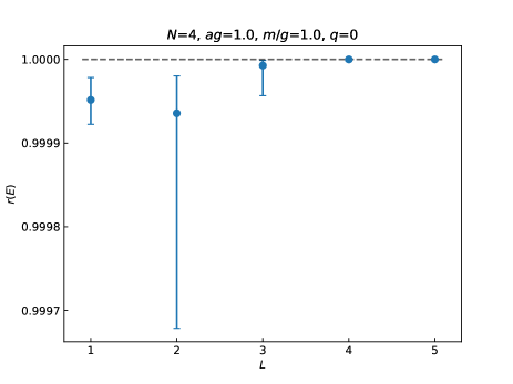
We first perform VQE for $N=4$, $ag=1$, $m/g=1$ in the absence of the external field $q=0$. We repeat optimizations $20$ times starting from different random initializations. Fig. 2 shows a metric of accuracy [102] $r(E):=(E_{\text{max}}-E_{\text{VQE}})/(E_{\text{max}}-E_{\text{min}})$ as a function of the number of layers, where $E_{\text{max/min}}$ is the highest/lowest eigenvalue of the Hamiltonian . The central value corresponds to the median of the 20 optimizations performed, while the error bar represents the 25-75 percentiles. One observes that high accuracy $r(E)\geq 0.999$ can be achieved for all $L$ and that for $L\geq 4$ the uncertainties improve markedly.

Figure 2: Ground state preparation via VQE: a metric of accuracy $r(E):=(E_{\text{max}}-E_{\text{VQE}})/(E_{\text{max}}-E_{\text{min}})$. Dots/error bars show the median and 25-75 percentiles of 20 samples.

IV.2 Quench dynamics via VQS

After preparing the initial state, we perform VQS for $N=4$, $ag=1$, $m/g=1$, and $q=2$ . First, we investigate the dependence of systematic errors on the number of layers $L$ and a time increment $\delta t$.

Figure 3: Fidelity between states from VQS and ED for $N=4,a\cdot g=1.0,m/g=1.0,q=2.0$. Solid curves/error bands show the medians and 25-75 percentiles of 20 samples: (left) dependence of the number of layers $L\in\{3,4,5\}$ with $\delta t=0.01$ fixed, (right) dependence of a time increment $\delta t\in\{0.01,0.02,0.04\}$ with $L$ fixed.

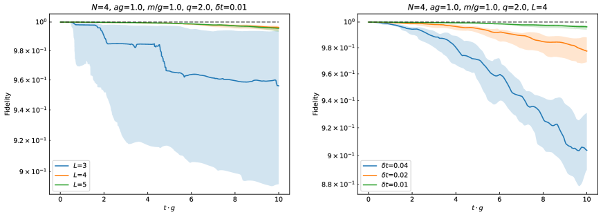
The left plot in Fig. 3 shows the fidelity $F(t):=\left\lvert\braket{\Psi_{\text{ED}}(t)}{\psi_{\text{VQS}}(t)}\right\rvert^{2}$ between the states obtained from VQS and ED as a function of (coupling constant times) time for different number of layers. One can see again that the uncertainty improves dramatically as the number of layers is raised above 3 and that for $L\geq 4$ the (median) fidelity is above $0.99$ and is improved by increasing the number of layers. The right panel shows the same plot, but this time varying $\delta t$ for fixed $L$. We see that the VQS results can be improved significantly by decreasing $\delta t$.

Next, we evaluate the physical observables discussed in Section II.2 and compare them to the results obtained by exact diagonalization. We verified that the U(1) charge agrees perfectly with the exact result, as can be expected since our Ansatz satisfies the global U(1) symmetry of the problem. The remaining two observables are shown in Fig. 4 with $L=5$ and $\delta t=0.01$ fixed.

Figure 4: Dynamics of physical observables for $N=4,a\cdot g=1.0,m/g=1.0,q=2.0$ with $L=5$ and $\delta=0.01$. Dots/error bars show the median and 25-75 percentiles of 20 samples: (a) electric field, (b) chiral condensate, (c), (d) ratio between the values of observables obtained from ED and VQS

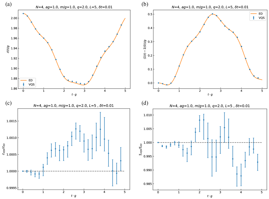
The VQS results are consistent with those from ED up to a few $\%$ errors. The errors from the variation over the 20 initial conditions is of the same order of magnitude as the difference from the exact result, but for the electric field and $1.5\lesssim t\cdot g\lesssim 4.5$ the difference between the exact result and the central value of the VQS results are about three times the size of the quoted error.

For $t\cdot g\lesssim 3$, the value of the electric field decreases while that of the chiral condensate increases, followed by the oscillation. This can be interpreted as follows: the external electric field first provides energy for fermions and then leads to particle pair creations.

V Summary and discussion

In this work, we demonstrated a possible application of the variational quantum algorithm to a gauge theory. Specifically, we investigated the real-time dynamics in the Schwinger model after suddenly turning on the external electric field, by combining VQE and VQS methods. We performed the (classically-emulated) state-vector simulation and found that the results obtained from the quantum algorithms are consistent with those obtained from ED. Our simulation results can be interpreted as a population of a particle-anti-particle pair induced by the external field.

There are many possible future directions. This paper used the original algorithm proposed by Li and Benjamin [65]. There are two main drawbacks to this approach: First, the matrix $M$ can be singular or ill-conditioned in practice, leading to unstable trajectories. Workarounds such as regularization add a parameter that must be tuned. Secondly, computing the each entry of $M$ requires $O(N_{p}^{2})$ calls to the quantum computer where $N_{p}$ is the number of parameters. There are many attempts to overcome this problem [70, 71, 72, 73, 74, 75, 76, 77, 78, 79, 80, 81, 82]. It would be important to see if these methods can improve our simulation results in terms of accuracy and measurement cost.

Toward an implementation on real quantum devices, it is important to understand the effects of hardware noise and statistical error coming from a finite number of measurements. Besides, combination with error mitigation methods can be an essential ingredient.

Finally, it would be interesting to consider an extension to the higher dimensional and/or non-Abelian gauge theory. For this purpose, a careful search for an Ansatz that is efficient and preserves gauge invariance during simulation can be crucial.

Appendix A McLachlan’s variational principle

This variational principle starts from a variational Ansatz state $\ket{\psi(\lambda)}$ given as the output of a parameterized circuit (and a global phase $\lambda_{0}$),

$$\ket{\psi(\lambda)}=e^{i\lambda_{0}(t)}\prod\limits_{i=1}^{N_{p}}U(\lambda_{i}(t))\ket{0}\,.$$ (35)

In other words, the time dependence of the state is encoded through the time dependence of the parameters $\lambda(t)$. The task of simulating Schrödinger evolution $\ket{\Psi(t)}=\mathcal{T}e^{-i\int H(s)ds}\ket{\Psi(0)}$ under a general, time-dependent Hamiltonian $H(t)$ using the Ansatz state $\ket{\psi(\lambda)}$ reduces to finding the parameter function $\lambda(t)$ such that at any time $t$, the state $\ket{\psi(\lambda(t))}$ optimally approximates the exact state $\ket{\Psi(t)}$.

A standard approach to this problem is to use a dynamical variational principle such as the McLachlan’s variational principle, or MVP for short. Other choices such as the Dirac-Frenkel variational principle and the time-dependent variational principle exist, and while different in subtle ways, they all agree under certain mild assumptions. In this section we focus on the MVP.

The central idea behind MVP is to minimize the difference between the rates of change of $\ket{\psi}$ under exact Hamiltonian evolution and variational evolution due to ${\rm d}\lambda/{\rm d}t$. Normally, this is expressed as minimizing the variation of the norm difference shown below,

$$\delta\left\lVert\left(\frac{d}{dt}+iH\right)\ket{\psi(\lambda(t))}\right\rVert^{2}=0$$ (36)

where $\left\lVert\cdot\right\rVert$ is the $l_{2}$-norm. Note that the variation in the above is with respect to $\delta({\rm d}\lambda_{i}/{\rm d}t)$, i.e., total time derivatives in each parameter $\lambda_{i}$. In other words, one is looking for stationary points by varying the tangent vector ${\rm d}\lambda/{\rm d}t$. Since one is dealing with a time-dependent Hamiltonian, the equation has to be written a little more carefully as

$$\lim_{\Delta t\rightarrow 0}\delta\frac{\left\lVert(U(t+\Delta t,t)-I)\ket{\psi}-\Delta t\ket{\dot{\psi}}\right\rVert^{2}}{\Delta t^{2}}=0\,,$$ (37)

where $U(t^{\prime},t):=\mathcal{T}e^{-i\int_{t}^{t^{\prime}}H(s)ds}$ and $I$ is the identity matrix. The main difference from the time-independent case is due to the appearance of an extra term at order $\Delta t^{2}$ due to the time dependence of $H$,

$$U(t+\Delta t,t) =I-iH\Delta t-(H^{2}+i\dot{H})\frac{\Delta t^{2}}{2}+O(\Delta t^{3})$$ (38)

$$\equiv U_{TI}(t+\Delta t,t)-i\dot{H}\frac{\Delta t^{2}}{2}+O(\Delta t^{3})$$ (39)

where $U_{TI}$ is the propagator if $H$ were held constant in time at the value $H(t)$. However, since the limit is insensitive to terms above linear order, the time-dependence of $H$ can be safely ignored.

Before expanding (36), one can implement some constraints on $\ket{\psi}$ and its time derivatives due to the normalization condition $\braket{\psi}{\psi}=1$. Setting the first and second time derivatives to zero yields, respectively,

$$\braket{\dot{\psi}}{\psi} =-\braket{\psi}{\dot{\psi}}$$ (40)

$$\operatorname{Re}\braket{\ddot{\psi}}{\psi} =-\braket{\dot{\psi}}{\dot{\psi}}\,.$$ (41)

Now, one expands the norm of the difference vector,

$$\left\lVert\ket{\dot{\psi}}+iH\ket{\psi}\right\rVert^{2} =\left(\bra{\dot{\psi}}-i\bra{\psi}H\right)\left(\ket{\dot{\psi}}+iH\ket{\psi}\right)$$ (42)

$$=\braket{\dot{\psi}}{\dot{\psi}}-2\operatorname{Im}\braket{\psi}{H}{\dot{\psi}}+\braket{H^{2}}\,,$$ (43)

using the notation $\braket{O}=\braket{\psi}{O}{\psi}$. Next, one writes $\ket{\dot{\psi}}$ in terms of partial derivatives

$$\ket{\dot{\psi}}=\dot{\lambda}_{0}\frac{\partial}{\partial\lambda_{0}}\ket{\psi}+\sum\limits_{i=1}^{N_{p}}\dot{\lambda}_{i}\frac{\partial}{\partial\lambda_{i}}\ket{\psi}=i\dot{\lambda}_{0}\ket{\psi}+\dot{\lambda}_{i}\ket{\partial_{i}\psi}\,,$$ (44)

where $\ket{\partial_{i}\psi}=\frac{\partial}{\partial\lambda_{i}}\ket{\psi}$. The last expression is implicitly summed over $i$ from $1$ to $N_{p}$, and the $i=0$ term (corresponding to global phase) gives a derivative parallel to $\ket{\psi}$. The purpose of the $\lambda_{0}$ term is to keep track of variations parallel to $\psi$ which do not change the overall state but can have an effect on the dynamics of the variational parameters. In practice, including it can lead to more well-behaved dynamics.

Then, one can separately express the terms containing $\ket{\dot{\psi}}$ as

$$\braket{\dot{\psi}}{\dot{\psi}} =\dot{\lambda}_{i}\dot{\lambda}_{j}\operatorname{Re}\braket{\partial_{i}\psi}{\partial_{j}\psi}$$

$$\quad+\dot{\lambda}_{0}\dot{\lambda}_{i}\operatorname{Im}\braket{\psi}{\partial_{i}\psi}+\dot{\lambda}_{0}^{2}\,,$$ (45)

$$\operatorname{Im}\braket{\psi}{H}{\dot{\psi}} =\dot{\lambda}_{0}\braket{H}+\dot{\lambda}_{i}\operatorname{Im}\braket{\psi}{H}{\partial_{i}\psi}\,,$$ (46)

where the properties $\braket{\psi}{\psi}=1$ and $\braket{\psi}{H}{\psi}=\braket{H}$ is real have been used. Taken together, this yields

$$\left\lVert\ket{\dot{\psi}}+iH\ket{\psi}\right\rVert^{2} =\dot{\lambda}_{i}\dot{\lambda}_{j}\operatorname{Re}\braket{\partial_{i}\psi}{\partial_{j}\psi}+\dot{\lambda}_{0}\dot{\lambda}_{i}\operatorname{Im}\braket{\psi}{\partial_{i}\psi}$$

$$\quad+\dot{\lambda}_{0}^{2}-2\dot{\lambda}_{0}\braket{H}-2\dot{\lambda}_{i}\operatorname{Im}\braket{\psi}{H}{\partial_{i}\psi}$$

$$\quad+\braket{H^{2}}\,,$$ (47)

$$=\dot{\lambda}_{i}\dot{\lambda}_{j}\operatorname{Re}\braket{\partial_{i}\psi}{\partial_{j}\psi}+\dot{\lambda}_{0}\dot{\lambda}_{i}\operatorname{Im}\braket{\psi}{\partial_{i}\psi}$$

$$\quad-2\dot{\lambda}_{i}\operatorname{Im}\braket{\psi}{H}{\partial_{i}\psi}+\left(\dot{\lambda}_{0}-\braket{H}\right)^{2}$$

$$\quad+\sigma^{2}_{\psi}(H)\,,$$ (48)

where $\sigma^{2}_{\psi}(H):=\braket{H^{2}}-\braket{H}^{2}$ is the variance of $H$ in the state $\ket{\psi}$. Now one derives stationary conditions by setting the derivatives in $\dot{\lambda}_{0}$ and each $\dot{\lambda}_{i}$ to 0. The first condition gives

$$\dot{\lambda}_{0}=\braket{H}+\dot{\lambda}_{i}\operatorname{Im}\braket{\psi}{\partial_{i}\psi}\,,$$ (49)

while the remaining conditions in each $i$ are given by

$$\dot{\lambda}_{j}\operatorname{Re}\braket{\partial_{i}\psi}{\partial_{j}\psi}+\dot{\lambda}_{0}\operatorname{Im}\braket{\psi}{\partial_{i}\psi}-\operatorname{Im}\braket{\psi}{H}{\partial_{i}\psi}=0$$ (50)

Substituting for $\dot{\lambda}_{0}$, and defining the projection operators $Q_{\psi}:=I-\ket{\psi}{\bra{\psi}}=:I-P_{\psi}$, one arrives at the final expression

$$\left(\operatorname{Re}\braket{\partial_{i}\psi}{Q_{\psi}}{\partial_{j}\psi}\right)\dot{\lambda}_{j}=\left(\operatorname{Im}\braket{\psi}{HQ_{\psi}}{\partial_{i}\psi}\right)\,.$$ (51)

The matrix $M_{ij}:=\operatorname{Re}\braket{\partial_{i}\psi}{Q_{\psi}}{\partial_{j}\psi}$ and vector $V_{i}:=\operatorname{Im}\braket{\psi}{HQ_{\psi}}{\psi}$ specify a linear system whose solutions give the McLachlan update vectors $\dot{\lambda}_{i}$ in each direction. Note that, while trivial, the global phase evolution can also be tracked via (49).

References

- [1] S. P. Jordan, K. S. M. Lee, and J. Preskill, “Quantum Algorithms for Quantum Field Theories,” Science 336 (2012) 1130–1133, arXiv:1111.3633 [quant-ph].
- [2] S. P. Jordan, K. S. M. Lee, and J. Preskill, “Quantum Computation of Scattering in Scalar Quantum Field Theories,” arXiv:1112.4833 [hep-th]. [Quant. Inf. Comput.14,1014(2014)].
- [3] S. P. Jordan, K. S. M. Lee, and J. Preskill, “Quantum Algorithms for Fermionic Quantum Field Theories,” arXiv:1404.7115 [hep-th].
- [4] E. A. Martinez et al., “Real-time dynamics of lattice gauge theories with a few-qubit quantum computer,” Nature 534 (2016) 516–519, arXiv:1605.04570 [quant-ph].
- [5] C. Muschik, M. Heyl, E. Martinez, T. Monz, P. Schindler, B. Vogell, M. Dalmonte, P. Hauke, R. Blatt, and P. Zoller, “U(1) Wilson lattice gauge theories in digital quantum simulators,” New J. Phys. 19 no. 10, (2017) 103020, arXiv:1612.08653 [quant-ph].
- [6] N. Klco, E. F. Dumitrescu, A. J. McCaskey, T. D. Morris, R. C. Pooser, M. Sanz, E. Solano, P. Lougovski, and M. J. Savage, “Quantum-classical computation of Schwinger model dynamics using quantum computers,” Phys. Rev. A98 no. 3, (2018) 032331, arXiv:1803.03326 [quant-ph].
- [7] C. Kokail et al., “Self-verifying variational quantum simulation of lattice models,” Nature 569 no. 7756, (2019) 355–360, arXiv:1810.03421 [quant-ph].
- [8] G. Magnifico, M. Dalmonte, P. Facchi, S. Pascazio, F. V. Pepe, and E. Ercolessi, “Real Time Dynamics and Confinement in the Schwinger-Weyl lattice model for 1+1 QED,” arXiv:1909.04821 [quant-ph].
- [9] B. Chakraborty, M. Honda, T. Izubuchi, Y. Kikuchi, and A. Tomiya, “Digital Quantum Simulation of the Schwinger Model with Topological Term via Adiabatic State Preparation,” arXiv:2001.00485 [hep-lat].
- [10] M. Honda, E. Itou, Y. Kikuchi, L. Nagano, and T. Okuda, “Classically emulated digital quantum simulation for screening and confinement in the schwinger model with a topological term,” Phys. Rev. D 105 (Jan, 2022) 014504. https://link.aps.org/doi/10.1103/PhysRevD.105.014504.
- [11] M. Honda, E. Itou, Y. Kikuchi, and Y. Tanizaki, “Negative string tension of a higher-charge Schwinger model via digital quantum simulation,” Progress of Theoretical and Experimental Physics 2022 no. 3, (Mar., 2022) 033B01, arXiv:2110.14105 [hep-th].
- [12] W. A. de Jong, K. Lee, J. Mulligan, M. Płoskoń, F. Ringer, and X. Yao, “Quantum simulation of non-equilibrium dynamics and thermalization in the Schwinger model,” arXiv e-prints (June, 2021) arXiv:2106.08394, arXiv:2106.08394 [quant-ph].
- [13] A. Yamamoto, “Quantum variational approach to lattice gauge theory at nonzero density,” arXiv:2104.10669 [hep-lat].
- [14] D. E. Kharzeev and Y. Kikuchi, “Real-time chiral dynamics from a digital quantum simulation,” Physical Review Research 2 no. 2, (June, 2020) 023342, arXiv:2001.00698 [hep-ph].
- [15] E. Gustafson, P. Dreher, Z. Hang, and Y. Meurice, “Real time evolution of a one-dimensional field theory on a 20 qubit machine,” arXiv:1910.09478 [hep-lat].
- [16] E. J. Gustafson and H. Lamm, “Toward quantum simulations of Z2 gauge theory without state preparation,” Phys. Rev. D 103 no. 5, (Mar., 2021) 054507, arXiv:2011.11677 [hep-lat].
- [17] A. F. Shaw, P. Lougovski, J. R. Stryker, and N. Wiebe, “Quantum Algorithms for Simulating the Lattice Schwinger Model,” Quantum 4 (Aug., 2020) 306, arXiv:2002.11146 [quant-ph].
- [18] D. Banerjee, S. Caspar, F.-J. Jiang, J.-H. Peng, and U.-J. Wiese, “Nematic confined phases in the u(1) quantum link model on a triangular lattice: Near-term quantum computations of string dynamics on a chip,” Phys. Rev. Res. 4 (Jun, 2022) 023176. https://link.aps.org/doi/10.1103/PhysRevResearch.4.023176.
- [19] QuNu Collaboration Collaboration, X.-D. Xie, X. Guo, H. Xing, Z.-Y. Xue, D.-B. Zhang, and S.-L. Zhu, “Variational thermal quantum simulation of the lattice schwinger model,” Phys. Rev. D 106 (Sep, 2022) 054509. https://link.aps.org/doi/10.1103/PhysRevD.106.054509.
- [20] N. H. Nguyen, M. C. Tran, Y. Zhu, A. M. Green, C. H. Alderete, Z. Davoudi, and N. M. Linke, “Digital quantum simulation of the schwinger model and symmetry protection with trapped ions,” PRX Quantum 3 (May, 2022) 020324. https://link.aps.org/doi/10.1103/PRXQuantum.3.020324.
- [21] A. Tomiya, “Schwinger model at finite temperature and density with beta VQE,” arXiv e-prints (May, 2022) arXiv:2205.08860, arXiv:2205.08860 [hep-lat].
- [22] A. N. Ciavarella and I. A. Chernyshev, “Preparation of the su(3) lattice yang-mills vacuum with variational quantum methods,” Phys. Rev. D 105 (Apr, 2022) 074504. https://link.aps.org/doi/10.1103/PhysRevD.105.074504.
- [23] Y. Atas, J. Zhang, R. Lewis, A. Jahanpour, J. F. Haase, and C. A. Muschik, “SU(2) hadrons on a quantum computer,” arXiv e-prints (Feb., 2021) arXiv:2102.08920, arXiv:2102.08920 [quant-ph].
- [24] Y. Y. Atas, J. F. Haase, J. Zhang, V. Wei, S. M. L. Pfaendler, R. Lewis, and C. A. Muschik, “Real-time evolution of SU(3) hadrons on a quantum computer,” arXiv e-prints (July, 2022) arXiv:2207.03473, arXiv:2207.03473 [quant-ph].
- [25] A. Mezzacapo, E. Rico, C. Sabin, I. L. Egusquiza, L. Lamata, and E. Solano, “Non-Abelian Lattice Gauge Theories in Superconducting Circuits,” Phys. Rev. Lett. 115 no. 24, (2015) 240502, arXiv:1505.04720 [quant-ph].
- [26] D. Marcos, P. Widmer, E. Rico, M. Hafezi, P. Rabl, U. J. Wiese, and P. Zoller, “Two-dimensional Lattice Gauge Theories with Superconducting Quantum Circuits,” Annals Phys. 351 (2014) 634–654, arXiv:1407.6066 [quant-ph].
- [27] N. Klco, J. R. Stryker, and M. J. Savage, “SU(2) non-Abelian gauge field theory in one dimension on digital quantum computers,” arXiv:1908.06935 [quant-ph].
- [28] A. Ciavarella, N. Klco, and M. J. Savage, “Trailhead for quantum simulation of SU(3) Yang-Mills lattice gauge theory in the local multiplet basis,” Phys. Rev. D 103 no. 9, (May, 2021) 094501, arXiv:2101.10227 [quant-ph].
- [29] G. Clemente, A. Crippa, and K. Jansen, “Strategies for the determination of the running coupling of ()-dimensional qed with quantum computing,” Phys. Rev. D 106 (Dec, 2022) 114511. https://link.aps.org/doi/10.1103/PhysRevD.106.114511.
- [30] C. Kane, D. M. Grabowska, B. Nachman, and C. W. Bauer, “Efficient quantum implementation of 2+1 U(1) lattice gauge theories with Gauss law constraints,” arXiv e-prints (Nov., 2022) arXiv:2211.10497, arXiv:2211.10497 [quant-ph].
- [31] L. Lumia, P. Torta, G. B. Mbeng, G. E. Santoro, E. Ercolessi, M. Burrello, and M. M. Wauters, “Two-dimensional lattice gauge theory on a near-term quantum simulator: Variational quantum optimization, confinement, and topological order,” PRX Quantum 3 (Apr, 2022) 020320. https://link.aps.org/doi/10.1103/PRXQuantum.3.020320.
- [32] D. Paulson, L. Dellantonio, J. F. Haase, A. Celi, A. Kan, A. Jena, C. Kokail, R. van Bijnen, K. Jansen, P. Zoller, and C. A. Muschik, “Simulating 2D Effects in Lattice Gauge Theories on a Quantum Computer,” PRX Quantum 2 no. 3, (Aug., 2021) 030334, arXiv:2008.09252 [quant-ph].
- [33] N. Klco and M. J. Savage, “Digitization of scalar fields for quantum computing,” Phys. Rev. A99 no. 5, (2019) 052335, arXiv:1808.10378 [quant-ph].
- [34] J. Barata, N. Mueller, A. Tarasov, and R. Venugopalan, “Single-particle digitization strategy for quantum computation of a 4 scalar field theory,” Phys. Rev. A 103 no. 4, (Apr., 2021) 042410, arXiv:2012.00020 [hep-th].
- [35] L. Garcia-Alvarez, J. Casanova, A. Mezzacapo, I. L. Egusquiza, L. Lamata, G. Romero, and E. Solano, “Fermion-Fermion Scattering in Quantum Field Theory with Superconducting Circuits,” Phys. Rev. Lett. 114 no. 7, (2015) 070502, arXiv:1404.2868 [quant-ph].
- [36] U.-J. Wiese, “Towards Quantum Simulating QCD,” Nucl. Phys. A931 (2014) 246–256, arXiv:1409.7414 [hep-th].
- [37] E. Gustafson, Y. Meurice, and J. Unmuth-Yockey, “Quantum simulation of scattering in the quantum Ising model,” Phys. Rev. D99 no. 9, (2019) 094503, arXiv:1901.05944 [hep-lat].
- [38] A. Kan and Y. Nam, “Lattice Quantum Chromodynamics and Electrodynamics on a Universal Quantum Computer,” arXiv e-prints (July, 2021) arXiv:2107.12769, arXiv:2107.12769 [quant-ph].
- [39] G. Pardo, T. Greenberg, A. Fortinsky, N. Katz, and E. Zohar, “Resource-Efficient Quantum Simulation of Lattice Gauge Theories in Arbitrary Dimensions: Solving for Gauss’ Law and Fermion Elimination,” arXiv e-prints (June, 2022) arXiv:2206.00685, arXiv:2206.00685 [quant-ph].
- [40] E. J. Gustafson, “Stout Smearing on a Quantum Computer,” arXiv e-prints (Nov., 2022) arXiv:2211.05607, arXiv:2211.05607 [hep-lat].
- [41] M. G. Echevarria, I. L. Egusquiza, E. Rico, and G. Schnell, “Quantum simulation of light-front parton correlators,” Phys. Rev. D 104 no. 1, (July, 2021) 014512, arXiv:2011.01275 [quant-ph].
- [42] Y. Su, H.-Y. Huang, and E. T. Campbell, “Nearly tight Trotterization of interacting electrons,” arXiv e-prints (Dec., 2020) arXiv:2012.09194, arXiv:2012.09194 [quant-ph].
- [43] J. Liu and Y. Xin, “Quantum simulation of quantum field theories as quantum chemistry,” Journal of High Energy Physics 2020 no. 12, (Dec., 2020) 11, arXiv:2004.13234 [hep-th].
- [44] A. J. Buser, H. Gharibyan, M. Hanada, M. Honda, and J. Liu, “Quantum simulation of gauge theory via orbifold lattice,” arXiv e-prints (Nov., 2020) arXiv:2011.06576, arXiv:2011.06576 [hep-th].
- [45] N. Klco and M. J. Savage, “Fixed-point quantum circuits for quantum field theories,” Phys. Rev. A 102 no. 5, (Nov., 2020) 052422, arXiv:2002.02018 [quant-ph].
- [46] N. Klco and M. J. Savage, “Minimally-Entangled State Preparation of Localized Wavefunctions on Quantum Computers,” arXiv:1904.10440 [quant-ph].
- [47] M. Asaduzzaman, G. C. Toga, S. Catterall, Y. Meurice, and R. Sakai, “Quantum simulation of the -flavor gross-neveu model,” Phys. Rev. D 106 (Dec, 2022) 114515. https://link.aps.org/doi/10.1103/PhysRevD.106.114515.
- [48] Z. Davoudi, A. F. Shaw, and J. R. Stryker, “General quantum algorithms for Hamiltonian simulation with applications to a non-Abelian lattice gauge theory,” arXiv e-prints (Dec., 2022) arXiv:2212.14030, arXiv:2212.14030 [hep-lat].
- [49] Z. Davoudi, I. Raychowdhury, and A. Shaw, “Search for efficient formulations for Hamiltonian simulation of non-Abelian lattice gauge theories,” Phys. Rev. D 104 no. 7, (Oct., 2021) 074505, arXiv:2009.11802 [hep-lat].
- [50] Z. Davoudi, N. Mueller, and C. Powers, “Toward Quantum Computing Phase Diagrams of Gauge Theories with Thermal Pure Quantum States,” arXiv e-prints (Aug., 2022) arXiv:2208.13112, arXiv:2208.13112 [hep-lat].
- [51] J. R. Stryker, “Shearing approach to gauge invariant Trotterization,” arXiv e-prints (May, 2021) arXiv:2105.11548, arXiv:2105.11548 [hep-lat].
- [52] A. Yamamoto and T. Doi, “Toward nuclear physics from lattice QCD on quantum computers,” arXiv e-prints (Nov., 2022) arXiv:2211.14550, arXiv:2211.14550 [hep-lat].
- [53] C. W. Bauer, B. Nachman, and M. Freytsis, “Simulating Collider Physics on Quantum Computers Using Effective Field Theories,” Phys. Rev. Lett. 127 no. 21, (Nov., 2021) 212001, arXiv:2102.05044 [hep-ph].
- [54] J. Liu and Y.-Z. Li, “Quantum simulation of cosmic inflation,” Phys. Rev. D 104 no. 8, (Oct., 2021) 086013, arXiv:2009.10921 [quant-ph].
- [55] H. Gharibyan, M. Hanada, M. Honda, and J. Liu, “Toward simulating superstring/M-theory on a quantum computer,” Journal of High Energy Physics 2021 no. 7, (July, 2021) 140, arXiv:2011.06573 [hep-th].
- [56] F. Mei, Q. Guo, Y.-F. Yu, L. Xiao, S.-L. Zhu, and S. Jia, “Digital Simulation of Topological Matter on Programmable Quantum Processors,” Phys. Rev. Lett. 125 no. 16, (Oct., 2020) 160503, arXiv:2003.06086 [quant-ph].
- [57] F. Arute et al., “Observation of separated dynamics of charge and spin in the Fermi-Hubbard model,” arXiv e-prints (Oct., 2020) arXiv:2010.07965, arXiv:2010.07965 [quant-ph].
- [58] NuQS Collaboration, H. Lamm, S. Lawrence, and Y. Yamauchi, “Parton Physics on a Quantum Computer,” arXiv:1908.10439 [hep-lat].
- [59] N. Mueller, A. Tarasov, and R. Venugopalan, “Deeply inelastic scattering structure functions on a hybrid quantum computer,” arXiv:1908.07051 [hep-th].
- [60] A. J. Buser, T. Bhattacharya, L. Cincio, and R. Gupta, “State preparation and measurement in a quantum simulation of the O(3) sigma model,” arXiv e-prints (June, 2020) arXiv:2006.15746, arXiv:2006.15746 [quant-ph].
- [61] H. Lamm and S. Lawrence, “Simulation of Nonequilibrium Dynamics on a Quantum Computer,” Phys. Rev. Lett. 121 no. 17, (2018) 170501, arXiv:1806.06649 [quant-ph].
- [62] NuQS Collaboration, A. Alexandru, P. F. Bedaque, H. Lamm, and S. Lawrence, “ Models on Quantum Computers,” Phys. Rev. Lett. 123 no. 9, (2019) 090501, arXiv:1903.06577 [hep-lat].
- [63] A. Macridin, P. Spentzouris, J. Amundson, and R. Harnik, “Electron-Phonon Systems on a Universal Quantum Computer,” Phys. Rev. Lett. 121 no. 11, (2018) 110504, arXiv:1802.07347 [quant-ph].
- [64] M. Motta, C. Sun, A. T. Tan, M. J. O’Rourke, E. Ye, A. J. Minnich, F. G. Brandão, and G. K.-L. Chan, “Determining eigenstates and thermal states on a quantum computer using quantum imaginary time evolution,” Nature Physics 16 no. 2, (2020) 205–210.
- [65] Y. Li and S. C. Benjamin, “Efficient variational quantum simulator incorporating active error minimization,” Physical Review X 7 no. 2, (2017) 021050.
- [66] X. Yuan, S. Endo, Q. Zhao, Y. Li, and S. C. Benjamin, “Theory of variational quantum simulation,” Quantum 3 (2019) 191.
- [67] S. Endo, J. Sun, Y. Li, S. C. Benjamin, and X. Yuan, “Variational quantum simulation of general processes,” Phys. Rev. Lett. 125 (Jun, 2020) 010501. https://link.aps.org/doi/10.1103/PhysRevLett.125.010501.
- [68] S. Endo, I. Kurata, and Y. O. Nakagawa, “Calculation of the green’s function on near-term quantum computers,” Phys. Rev. Res. 2 (Aug, 2020) 033281. https://link.aps.org/doi/10.1103/PhysRevResearch.2.033281.
- [69] Y.-X. Yao, N. Gomes, F. Zhang, C.-Z. Wang, K.-M. Ho, T. Iadecola, and P. P. Orth, “Adaptive variational quantum dynamics simulations,” PRX Quantum 2 (Jul, 2021) 030307. https://link.aps.org/doi/10.1103/PRXQuantum.2.030307.
- [70] C. Cîrstoiu, Z. Holmes, J. Iosue, L. Cincio, P. J. Coles, and A. Sornborger, “Variational fast forwarding for quantum simulation beyond the coherence time,” npj Quantum Information 6 (Sept., 2020) 82, arXiv:1910.04292 [quant-ph].
- [71] J. Gibbs, K. Gili, Z. Holmes, B. Commeau, A. Arrasmith, L. Cincio, P. J. Coles, and A. Sornborger, “Long-time simulations for fixed input states on quantum hardware,” npj Quantum Information 8 (Jan., 2022) 135, arXiv:2102.04313 [quant-ph].
- [72] B. Commeau, M. Cerezo, Z. Holmes, L. Cincio, P. J. Coles, and A. Sornborger, “Variational Hamiltonian Diagonalization for Dynamical Quantum Simulation,” arXiv e-prints (Sept., 2020) arXiv:2009.02559, arXiv:2009.02559 [quant-ph].
- [73] M. Benedetti, M. Fiorentini, and M. Lubasch, “Hardware-efficient variational quantum algorithms for time evolution,” Physical Review Research 3 no. 3, (July, 2021) 033083, arXiv:2009.12361 [quant-ph].
- [74] S.-H. Lin, R. Dilip, A. G. Green, A. Smith, and F. Pollmann, “Real- and imaginary-time evolution with compressed quantum circuits,” PRX Quantum 2 (Mar, 2021) 010342. https://link.aps.org/doi/10.1103/PRXQuantum.2.010342.
- [75] F. Barratt, J. Dborin, M. Bal, V. Stojevic, F. Pollmann, and A. G. Green, “Parallel quantum simulation of large systems on small NISQ computers,” npj Quantum Information 7 (Jan., 2021) 79, arXiv:2003.12087 [quant-ph].
- [76] S. Barison, F. Vicentini, and G. Carleo, “An efficient quantum algorithm for the time evolution of parameterized circuits,” arXiv e-prints (Jan., 2021) arXiv:2101.04579, arXiv:2101.04579 [quant-ph].
- [77] K. Heya, K. M. Nakanishi, K. Mitarai, and K. Fujii, “Subspace Variational Quantum Simulator,” arXiv e-prints (Apr., 2019) arXiv:1904.08566, arXiv:1904.08566 [quant-ph].
- [78] L. Slattery, B. Villalonga, and B. K. Clark, “Unitary block optimization for variational quantum algorithms,” Physical Review Research 4 no. 2, (Apr., 2022) 023072, arXiv:2102.08403 [quant-ph].
- [79] K. Bharti and T. Haug, “Quantum-assisted simulator,” Phys. Rev. A 104 (Oct, 2021) 042418. https://link.aps.org/doi/10.1103/PhysRevA.104.042418.
- [80] J. W. Z. Lau, K. Bharti, T. Haug, and L. C. Kwek, “Noisy intermediate scale quantum simulation of time dependent Hamiltonians,” arXiv e-prints (Jan., 2021) arXiv:2101.07677, arXiv:2101.07677 [quant-ph].
- [81] J. W. Z. Lau, T. Haug, L. C. Kwek, and K. Bharti, “NISQ Algorithm for Hamiltonian simulation via truncated Taylor series,” SciPost Physics 12 no. 4, (Apr., 2022) 122, arXiv:2103.05500 [quant-ph].
- [82] S. Barison, F. Vicentini, I. Cirac, and G. Carleo, “Variational dynamics as a ground-state problem on a quantum computer,” Physical Review Research 4 no. 4, (Dec., 2022) 043161, arXiv:2204.03454 [quant-ph].
- [83] K. Wada, R. Raymond, Y.-y. Ohnishi, E. Kaminishi, M. Sugawara, N. Yamamoto, and H. C. Watanabe, “Simulating time evolution with fully optimized single-qubit gates on parametrized quantum circuits,” Phys. Rev. A 105 (Jun, 2022) 062421. https://link.aps.org/doi/10.1103/PhysRevA.105.062421.
- [84] A. Miessen, P. J. Ollitrault, F. Tacchino, and I. Tavernelli, “Quantum algorithms for quantum dynamics,” Nature Computational Science 3 no. 1, (2023) 25–37. https://doi.org/10.1038/s43588-022-00374-2.
- [85] J. Liu, Z. Li, H. Zheng, X. Yuan, and J. Sun, “Towards a variational Jordan-Lee-Preskill quantum algorithm,” Machine Learning: Science and Technology 3 no. 4, (Dec., 2022) 045030, arXiv:2109.05547 [quant-ph].
- [86] J. Schwinger, “On gauge invariance and vacuum polarization,” Phys. Rev. 82 (Jun, 1951) 664–679. https://link.aps.org/doi/10.1103/PhysRev.82.664.
- [87] B. Buyens, J. Haegeman, F. Hebenstreit, F. Verstraete, and K. Van Acoleyen, “Real-time simulation of the schwinger effect with matrix product states,” Physical Review D 96 no. 11, (2017) 114501.
- [88] B. Xu and W. Xue, “()-dimensional schwinger pair production with quantum computers,” Phys. Rev. D 106 (Dec, 2022) 116007. https://link.aps.org/doi/10.1103/PhysRevD.106.116007.
- [89] J. S. Schwinger, “Gauge Invariance and Mass. 2.,” Phys. Rev. 128 (1962) 2425–2429.
- [90] J. Lowenstein and J. Swieca, “Quantum electrodynamics in two dimensions,” Annals of Physics 68 no. 1, (1971) 172–195. https://www.sciencedirect.com/science/article/pii/0003491671902466.
- [91] S. R. Coleman, R. Jackiw, and L. Susskind, “Charge Shielding and Quark Confinement in the Massive Schwinger Model,” Annals Phys. 93 (1975) 267.
- [92] D. J. Gross, I. R. Klebanov, A. V. Matytsin, and A. V. Smilga, “Screening versus confinement in (1+1)-dimensions,” Nucl. Phys. B461 (1996) 109–130, arXiv:hep-th/9511104 [hep-th].
- [93] J. B. Kogut and L. Susskind, “Hamiltonian Formulation of Wilson’s Lattice Gauge Theories,” Phys. Rev. D11 (1975) 395–408.
- [94] P. Jordan and E. Wigner, “Über das paulische äquivalenzverbot,” Zeitschrift für Physik 47 no. 9, (Sep, 1928) 631–651. https://doi.org/10.1007/BF01331938.
- [95] L. Funcke, K. Jansen, and S. Kühn, “Topological vacuum structure of the schwinger model with matrix product states,” Physical Review D 101 no. 5, (2020) 054507.
- [96] D. Wecker, M. B. Hastings, and M. Troyer, “Progress towards practical quantum variational algorithms,” Phys. Rev. A 92 (Oct, 2015) 042303. https://link.aps.org/doi/10.1103/PhysRevA.92.042303.
- [97] W. W. Ho and T. H. Hsieh, “Efficient variational simulation of non-trivial quantum states,” SciPost Phys. 6 (2019) 029. https://scipost.org/10.21468/SciPostPhys.6.3.029.
- [98] R. Wiersema, C. Zhou, Y. de Sereville, J. F. Carrasquilla, Y. B. Kim, and H. Yuen, “Exploring entanglement and optimization within the hamiltonian variational ansatz,” PRX Quantum 1 (Dec, 2020) 020319. https://link.aps.org/doi/10.1103/PRXQuantum.1.020319.
- [99] A. D. McLachlan, “A variational solution of the time-dependent Schrodinger equation,” Molecular Physics 8 no. 1, (Jan., 1964) 39–44.
- [100] Y. Suzuki, Y. Kawase, Y. Masumura, Y. Hiraga, M. Nakadai, J. Chen, K. M. Nakanishi, K. Mitarai, R. Imai, S. Tamiya, T. Yamamoto, T. Yan, T. Kawakubo, Y. O. Nakagawa, Y. Ibe, Y. Zhang, H. Yamashita, H. Yoshimura, A. Hayashi, and K. Fujii, “Qulacs: a fast and versatile quantum circuit simulator for research purpose,” Quantum 5 (Oct., 2021) 559, arXiv:2011.13524 [quant-ph].
- [101] P. Weinberg and M. Bukov, “QuSpin: a Python package for dynamics and exact diagonalisation of quantum many body systems part I: spin chains,” SciPost Physics 2 no. 1, (Feb., 2017) 003, arXiv:1610.03042 [physics.comp-ph].
- [102] G. Pagano, A. Bapat, P. Becker, K. S. Collins, A. De, P. W. Hess, H. B. Kaplan, A. Kyprianidis, W. L. Tan, C. Baldwin, L. T. Brady, A. Deshpande, F. Liu, S. Jordan, A. V. Gorshkov, and C. Monroe, “Quantum approximate optimization of the long-range Ising model with a trapped-ion quantum simulator,” Proceedings of the National Academy of Science 117 no. 41, (Oct., 2020) 25396–25401, arXiv:1906.02700 [quant-ph].