An Implicit GNN Solver for Poisson-like problems

Abstract

This paper presents $\Psi$-GNN, a novel Graph Neural Network (GNN) approach for solving the ubiquitous Poisson PDE problems with mixed boundary conditions. By leveraging the Implicit Layer Theory, $\Psi$-GNN models an “infinitely” deep network, thus avoiding the empirical tuning of the number of required Message Passing layers to attain the solution. Its original architecture explicitly takes into account the boundary conditions, a critical pre-requisite for physical applications, and is able to adapt to any initially provided solution. $\Psi$-GNN is trained using a “physics-informed” loss, and the training process is stable by design, and insensitive to its initialization. Furthermore, the consistency of the approach is theoretically proven, and its flexibility and generalization efficiency are experimentally demonstrated: the same learned model can accurately handle unstructured meshes of various sizes, as well as different boundary conditions. To the best of our knowledge, $\Psi$-GNN is the first physics-informed GNN-based method that can handle various unstructured domains, boundary conditions and initial solutions while also providing convergence guarantees.

1 Introduction

Partial differential equations (PDEs) are highly detailed mathematical models that describe complex physical or artificial processes in engineering and science (Olver, 2013). Although they have been widely studied for many years, solving these equations at scale remains daunting, limited by the computational cost of resolving the smallest spatio-temporal scales (Morton & Mayers, 2005). One of the most common and important PDEs in engineering is the steady-state Poisson equation, mathematically described as $-\Delta u=f$ on some domain $\Omega\subset\mathbb{R}^{n}$ (usually, $n=2$ or $3$) and some forcing term $f$, where $u$ is the solution to be sought. The Poisson equation appears in various fields such as Gravity (Mannheim & Kazanas, 1994), Electrostatics (Luty et al., 1992), Surface reconstruction (Kazhdan et al., 2006), or Fluid mechanics (Guermond & Quartapelle, 1998). It is ubiquitous and plays a central role in modern numerical solvers. Despite progresses in the High-Performance Computing (HPC) community, solving large Poisson problems is achievable only by employing robust yet tedious iterative methods (Saad, 2003) and remains the major bottleneck in the speedup of industrial numerical simulations.

More recently, data-driven methods based on deep neural networks have been reshaping the domain of numerical simulation. Neural networks can provide faster predictions, reducing the turnaround time for workflows in engineering and science (Wiewel et al., 2019; Um et al., 2020; Kochkov et al., 2021) – see also our quick survey in Section 2. However, the lack of guarantees about the consistency and convergence of deep learning approaches makes it non-viable to implement these models in the design and production stage of new engineering solutions.

This work introduces $\Psi$-GNN, an Implicit Graph Neural Network (GNN) approach that iteratively solves a Poisson problem with mixed boundary conditions. Leveraging Implicit Layer Theory (Bai et al., 2019), the proposed model controls, by itself, the number of Message Passing layers needed to reach the solution, yielding excellent out-of-distribution generalization to mesh sizes and shapes. The $\Psi$-GNN architecture, detailed in Section 3, is based on a node-oriented approach, which inherently respects the boundary conditions, and an additional autoencoding process allows it to be flexible with respect to its initialization. The method is trained end-to-end, mainly minimizing the residual of the discretized Poisson problem, thus attempting to learn the physics of the problem; However, in practice, some additional lightly-weighted supervised loss (MSE with ground-truth solutions) is still necessary for convergence when Neumann conditions are present. To ensure the stability of the model, a regularized cost function (Bai et al., 2021) is used to constrain the spectral radius of the Machine Learning solver, thus providing strong convergence guarantees. We prove (Section 4) the consistency of the approach and demonstrate its generalization ability in Section 5 through experiments with various geometries and boundary conditions. We also discuss the complexity of $\Psi$-GNN to get insights into its performance and discuss its relation to state-of-the-art Machine Learning models.

2 Related Work

In the past few years, the use of Machine Learning models to predict solutions of PDEs has gained significant interest in the community, beginning in the 90s with pioneering work from Lee & Kang (1990) and Lagaris et al. (1998). Since then, much research has focused on building more complex neural network architectures with a larger number of parameters, taking advantage of increasing computational power as demonstrated in Smaoui & Al-Enezi (2004) or Kumar & Yadav (2011).

CNNs for physics simulations Despite these convincing advances that employed fully connected neural networks, these methods were quickly overtaken by the tremendous progress in computer vision and the rise of Convolutional Neural Networks (CNNs) (LeCun et al., 1995). Due to its engineering interest, a significant amount of research has focused on using CNNs to solve the Poisson equation, as demonstrated in Tang et al. (2017); Hsieh et al. (2019); Özbay et al. (2021) or Cheng et al. (2021). All these approaches have shown promising results, approximating solutions up to 30 times faster than classical solvers by taking advantage of the GPU parallelization offered in the Machine Learning area. Still, their application remains limited to structured grids with uniform discretization.

GNNs for physics simulations To address this shortcoming, recent studies have focused on Graph Neural Networks (GNNs) (Battaglia et al., 2016), a class of neural networks that can learn from unstructured data. Similar to CNN-oriented research, some studies have focused on using GNNs to solve the Poisson equation, starting with the work of Alet et al. (2019). Li et al. (2020) introduce a graph kernel network to approximate PDEs with a specific focus on the resolution of a 2D Poisson problem, and in Chen et al. (2022), a multi-level GNN architecture is trained through supervised learning to solve the Poisson Pressure equation in the context of fluid simulations. These approaches outperform the CNN-based models due to their generalization to unstructured grids. However, these methods rely mainly on supervised learning losses, and the absence of the physics of the problem hinders their performance on out-of-distribution examples. Additionally, the treatment of boundary conditions is often missing and remains a significant challenge for practical use in industrial processes.

The Physics-Informed approach  In parallel to these architectural advancements, another research direction focuses on a new class of Deep Learning method called Physics-Informed Neural Networks (PINNs), which has emerged as a very promising tool for solving scientific computational problems (Raissi & Karniadakis, 2018). These methods are mesh-free and specifically designed to integrate the PDE into the training loss. Numerous works have used this approach to solve more complex problems, such as in fluid mechanics as demonstrated in Wu et al. (2018); Jin et al. (2021), or Cai et al. (2022). Therefore, the approach of training a model by minimizing the residual equation is well known and has been combined with GNNs to build an autoregressive Machine Learning PDE solver (Brandstetter et al., 2022) or solve a 2D Poisson equation (Gao et al., 2022). However, our method is mesh-based and distinguished by its ability to generalize to different domains, boundary conditions and initial solutions.

Deep Statistical Solver  Our work is closely related to Donon et al. (2020), where a GNN is used to efficiently solve a Poisson problem with Dirichlet boundary conditions. We propose a novel GNN-based architecture that can handle mixed boundary conditions, making it extensible to CFD cases. In previous work, the number of Message Passing Neural Networks (MPNN) needed to achieve convergence was fixed, and it was proved that it had to be proportional to the largest diameter of meshes in the dataset for the approach to be consistent. Nastorg et al. (2022) further improve upon by introducing a Recurrent Graph architecture which significantly reduces the model size. Besides, they experimentally demonstrate that if the model is trained with sufficient MPNN iterations, it tends to converge toward a fixed point. However, the number of iterations remains fixed, and the model has poor generalization capabilities to different mesh sizes. To address this issue, we propose using Implicit Layer Theory (Bai et al., 2019) to model an infinitely deep neural network that controls the number of Message Passing steps to reach convergence.

3 Methodology

In this section, we provide a detailed methodology for the study, including problem statement 3.1, graph interpretation and statistical problem 3.2, model architecture 3.3, regularization technique 3.4 and training process 3.5.

3.1 Problem statement

Let $\Omega\subset\mathbb{R}^{n}$ be a bounded open domain with smooth boundary $\partial\Omega=\partial\Omega_{D}\cup\partial\Omega_{N}$. To ensure the existence and uniqueness of the solution, special constraints (referred to as boundary conditions) must be specified on the boundary $\partial\Omega$ of $\Omega$ (Langtangen & Mardal, 2019): Dirichlet conditions assign a known value for the solution $u$ on (part of) $\partial\Omega$, and homogeneous Neumann boundary conditions impose that no part of the solution $u$ is leaving the domain. More formally, let $f$ be a continuous function defined on $\Omega$, $g$ a continuous function defined on $\partial\Omega_{D}$ and $n$ the outward normal vector defined on $\partial\Omega$. The Poisson problem with mixed boundary conditions (i.e. Dirichlet and homogeneous Neumann boundary conditions) consists in finding a real-valued function $u$, defined on $\Omega$, that satisfies:

$$\left\{\begin{array}[]{rcl}-\Delta u&=&f\qquad\in\Omega\\ u&=&g\qquad\in\partial\Omega_{D}\\ \frac{\partial u}{\partial n}&=&0\qquad\in\partial\Omega_{N}\end{array}\right.$$ (1)

Except in very specific instances, no analytical solution can be derived for the Poisson problem, and its solution must be numerically approximated: the domain $\Omega$ is first discretized into an unstructured mesh, denoted $\Omega_{h}$. The Poisson equation (1) is then spatially discretized using the Finite Element Method (FEM) (Reddy, 2019). The approximate solution $u_{h}$ is sought as a vector of values defined on all $N$ degrees of freedom of $\Omega_{h}$. $N$ in turn depends on the type of elements chosen (i.e., the precision order of the approximation wanted): choosing first-order Lagrange elements, $N$ matches the number of nodes in $\Omega_{h}$. The discretization of the variational formulation with Galerkin’s method leads to solving a linear system of the form:

$$AU=B$$ (2)

where the sparse matrix $A\in\mathbb{R}^{N\times N}$ is the discretization of the continuous Laplace operator, vector $B\in\mathbb{R}^{N}$ comes from the discretization of the force term $f$ and of the mixed boundary conditions, and $U\in\mathbb{R}^{N}$ is the solution vector to be sought.

Let $\mathcal{F}$ be a set of continuous functions on $\Omega$ and $\mathcal{G}$ a set of continuous functions on $\partial\Omega_{D}$. We denote as $\mathcal{P}$ a set of Poisson problems, such that any element $E_{p}\in\mathcal{P}$ is described as a triplet:

$$E_{p}=\left(\Omega_{p},~{}f_{p},~{}g_{p}\right)$$

where $\Omega_{p}\subset\Omega$, $f_{p}\in\mathcal{F}$ and $g_{p}\in\mathcal{G}$. For all $E_{p}\in\mathcal{P}$, let $E_{h,p}\in\mathcal{P}_{h}$ denote its discretization, such that:

$$E_{h,p}=\left(\Omega_{h,p},~{}A_{p},~{}B_{p}\right)$$

where $\Omega_{h,p}\subset\Omega_{h}$ and $A_{p}$ and $B_{p}$ are defined as for Eq. (2).

The fundamental idea of $\Psi$-GNN is, considering a continuous Poisson problem $E_{p}\in\mathcal{P}$, to build a Machine Learning solver, parametrized by a vector $\theta$, which outputs a statistically correct solution $U_{p}$ of its respective discretized form $E_{h,p}\in\mathcal{P}_{h}$:

$$U_{p}~{}=~{}\textit{solver}_{\theta}\left(E_{h,p}\right)=~{}\textit{solver}_{\theta}\left(\Omega_{h,p},~{}A_{p},~{}B_{p}\right)$$ (3)

3.2 Statistical problem

In (2), it should be noted that the structure of matrix $A$ encodes the geometry of its corresponding mesh. Indeed, for each node, using first-order finite elements leads to the creation of local stencils, which represent local connections between mesh nodes. A crucial upside of using GNNs in physics simulations is related to the right treatment of boundary conditions. In (2), the Dirichlet boundary conditions break the symmetry of the matrix $A$. Therefore, we use a directed graph at those particular nodes, sending information only to its neighbours without receiving any. Conversely, Interior and Neumann nodes have bi-directional edges, thus exchanging information with each other until convergence. Figure 4 illustrates such a graph with the three types of nodes: Interior, Dirichlet and Neumann.

A discretized Poisson problem $E_{h}=\left(\Omega_{h},~{}A,~{}B\right)$ with $N$ degrees of freedom can be interpreted as a graph problem $G=(N,~{}A,~{}B)$, where $N$ is the number of nodes in the graph, $A=(a_{ij})_{(i,j)\in[N]^{2}}$ is the weighted adjacency matrix that represents the interactions between the nodes and $B=(b_{i})_{i\in[N]}$ is some local external input. Vector $U=(u_{i})_{i\in[N]}$ represents the state of the graph, $u_{i}$ being the state of node $i$. Let $\mathcal{S}$ be the set of all such graphs $G$, and $\mathcal{U}$ the set of all states $U$. By abuse of notation, we will write $\mathcal{S}=\mathcal{P}_{h}$.

Additionally, let $\mathcal{L}_{\text{res}}$ be the real-valued function which computes the mean square error (MSE) of the residual of the discretized equation:

$$\mathcal{L}_{\text{res}}(U,~{}G) =\text{MSE}\left(AU-B\right)$$ (4)

$$=\displaystyle\frac{1}{N}\sum_{i\in[N]}\Big{(}-b_{i}+\sum_{j\in[N]}a_{i,j}u_{j}\Big{)}^{2}$$ (5)

The intuitive problem is given a graph $G$ to find an optimal state in $\mathcal{U}$ that minimizes (5). More generally, we are interested in building a Machine Learning solver, parametrized by $\theta$, which finds such an optimal state for any graphs $G$ sampled from a given distribution $\mathcal{D}$ over $\mathcal{S}$. Hence, the statistical problem can be formulated as follows: Given a distribution $\mathcal{D}$ on space $\mathcal{S}$ and a loss function $\mathcal{L}$, solve:

$$\theta^{*}=\underset{{\theta}}{\text{argmin}}~{}\underset{G\sim\mathcal{D}}{\mathbb{E}}\left[\mathcal{L}_{\text{res}}\left(\textit{solver}_{\theta}\left(G\right),G\right)\right]$$ (6)

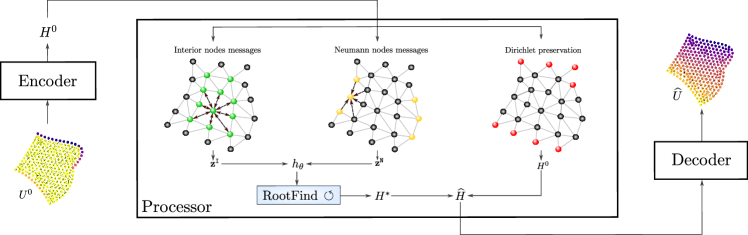
Figure 1: Diagram of $\Psi$-GNN: The model uses an Encode-Process-Decode architecture. The encoder maps an initial solution $U^{0}$ to some latent representation $H^{0}$. The processor outputs a final latent state $\widehat{H}$ by considering a different treatment for each node type. Specific MPNN for Interior and Neumann nodes are computed to build a GNN function $h_{\theta}$. A black-box “RootFind” solver automatically propagates the information through the graph by finding the fixed point $H^{*}$ of $h_{\theta}$. Dirichlet nodes are preserved during the process and combined with $H^{*}$ to get the final latent state $\widehat{H}$. The decoder maps $\widehat{H}$ back to the physical space to get the final solution $\widehat{U}$.

3.3 Architecture

Figure 1 gives a global view of $\Psi$-GNN, a Graph Neural Network model with three main components: an Encoder, a Processor, and a Decoder. The “Encoder-Decoder” mechanism facilitates the connection between the physical space, where the solution lives, and the latent space, where the GNN layers are applied. The Processor is the core component of the model, responsible for propagating the information correctly within the graph. It is specifically designed with two key features: i) automatically controls the number of Message Passing steps required for convergence; ii) properly takes into account the boundary conditions by design.

Encoder  The encoder $E_{\theta}$ maps an initial solution $U^{0}\in\mathcal{U}$ to a $d-$dimensional latent state $H^{0}\in\mathcal{H}$, $d>1$. The provided initial solution must fulfill the Dirichlet boundary conditions. This trainable function projects the physical space $\mathcal{U}$ to a higher dimensional latent space $\mathcal{H}$ on which the GNN layers will be applied.

Processor  The processor uses a specialized approach for each node type to ensure adherence to the boundary conditions. For Dirichlet boundary nodes, the corresponding latent variable is kept constant, equal to the imposed value. To propagate the information, the processor constructs a GNN-based function $h_{\theta}$ that takes into account messages for both the Interior and Neumann nodes, effectively capturing the distinct stencils of the discretized Laplace operator.

Interior nodes messages  Three separate messages are computed for each node, corresponding to the outgoing, incoming and self-loop links, using trainable functions $\Phi_{\rightarrow,\theta}^{\texttt{I}}$, $\Phi_{\leftarrow,\theta}^{\texttt{I}}$ and $\Phi_{\circlearrowleft,\theta}$:

$$\phi_{\rightarrow,i}^{\texttt{I}} =\displaystyle\sum_{j\in\mathcal{N}(i)}\Phi_{\rightarrow,\theta}^{\texttt{I}}\left(H_{i},H_{j},d_{ij}\right)$$ (7)

$$\phi_{\leftarrow,i}^{\texttt{I}} =\displaystyle\sum_{j\in\mathcal{N}(i)}\Phi_{\leftarrow,\theta}^{\texttt{I}}\left(H_{i},H_{j},d_{ji}\right)$$ (8)

$$\phi_{\circlearrowleft,i}^{\texttt{I}} =\displaystyle\Phi_{\circlearrowleft,\theta}\left(H_{i},t_{i}\right)$$ (9)

where $j\in\mathcal{N}(i)$ stands for all the nodes $j$ in the one-hop neighbourhood of $i$, $d_{ij}$ represents the euclidean distance between two nodes $i$ and $j$, and $t_{i}$ is a one-hot vector that differentiates node types.

To compute the updated Interior latent variable $\textbf{z}^{\texttt{I}}\coloneqq(z_{i}^{\texttt{I}})_{i\in[N]}$, messages (7), (8) and (9) are combined with problem-specific data $b_{i}$ (such as the discretized $f$ and $g$ functions from (1)) and passed through a modified GRU cell (Chung et al., 2014) as follows:

$$\alpha_{i} =\Psi^{1}_{\theta}\left(H_{i},b_{i},\phi_{\rightarrow,i}^{\texttt{I}},\phi_{\leftarrow,i}^{\texttt{I}},\phi_{\circlearrowleft,i}^{\texttt{I}}\right)$$ (10)

$$\beta_{i} =\Psi^{2}_{\theta}\left(H_{i},b_{i},\phi_{\rightarrow,i}^{\texttt{I}},\phi_{\leftarrow,i}^{\texttt{I}},\phi_{\circlearrowleft,i}^{\texttt{I}}\right)$$ (11)

$$\zeta_{i} =\Psi^{3}_{\theta}\left(\beta_{i}*H_{i},b_{i},\phi_{\rightarrow,i}^{\texttt{I}},\phi_{\leftarrow,i}^{\texttt{I}},\phi_{\circlearrowleft,i}^{\texttt{I}}\right)$$ (12)

$$z_{i}^{\texttt{I}} =H_{i}+\alpha_{i}*\zeta_{i}$$ (13)

where $\Psi^{1}_{\theta}$, $\Psi^{2}_{\theta}$ and $\Psi^{3}_{\theta}$ are trainable functions. Figure 5 from Appendix A displays this specific architecture, which is responsible for the flow of information within the Interior nodes of the graph.

Neumann nodes messages  Two distinct messages are computed: one from an incoming link and the other from a self-loop link, both designed to capture the stencil that ensures homogeneous Neumann boundary conditions. They are constructed in a similar manner to (8) and (9), using trainable functions $\Phi_{\leftarrow,\theta}^{\texttt{N}}$ and $\Phi_{\circlearrowleft,\theta}$:

$$\phi_{\leftarrow,i}^{\texttt{N}} =\displaystyle\sum_{j\in\mathcal{N}(i)}\Phi_{\leftarrow,\theta}^{\texttt{N}}\left(H_{i},H_{j},d_{ji}\right)$$ (14)

$$\phi_{\circlearrowleft,i}^{\texttt{N}} =\displaystyle\Phi_{\circlearrowleft,\theta}\left(H_{i},t_{i}\right)$$ (15)

The updated Neumann latent variable $\textbf{z}^{\texttt{N}}\coloneqq(z_{i}^{\texttt{N}})_{i\in[N]}$ is computed by combining messages (14) and (15) with problem-related data $b_{i}$ and the information on the normal vector $n_{i}$, and passing the result through a trainable function $\Psi^{4}_{\theta}$ as follows:

$$z_{i}^{\texttt{N}} =\Psi^{4}_{\theta}\left(H_{i},b_{i},n_{i},\phi_{\leftarrow,i}^{\texttt{N}},\phi_{\circlearrowleft,i}^{\texttt{N}}\right)$$ (16)

The GNN-based function $h_{\theta}$ is designed to separate the Interior and Neumann messages and is given by:

$$h_{\theta}(H,G)=\text{LN}\Big{(}\Big{[}\textbf{z}^{\texttt{I}},~{}\textbf{z}^{\texttt{N}}\Big{]}\Big{)}$$ (17)

where LN stands for the Layer Normalization operation (Ba et al., 2016).

Fixed-point problem One step of message passing only propagates information from one node to its immediate neighbours. In order to propagate information throughout the graph, previous works (Nastorg et al., 2022) repeatedly performed the message passing step, i.e., looped over the function $h_{\theta}$, either for a fixed number of iterations or until the problem converges. Iterating until convergence amounts to solving a fixed-point problem $H^{*}=h_{\theta}\left(H^{*},~{}G\right)$. Hence we propose to leverage Implicit Layer Theory and to use some black-box RootFind procedure to directly solve the fixed-point problem:

$$H^{*}=\text{RootFind}\left(h_{\theta}\left(H,~{}G\right)-H\right)$$ (18)

This approach eliminates the need for a pre-defined number of iterations of $h_{\theta}$ and only requires a threshold precision of the RootFind solver, resulting in a more adaptable and flexible approach. To solve Equation (18), Newton’s methods are the methods of choice, thanks to their fast convergence guarantees. However, to avoid the costly computation of the inverse Jacobian at each Newton iteration, we will use the quasi-Newton Broyden algorithm (Broyden, 1965), which uses low-rank updates to maintain an approximation of the Jacobian.

Final latent state The final latent variable $\widehat{H}$ is obtained by combining the output $H^{*}$ from the “Interior-Neumann” process with the initial latent state $H^{0}$, which was held constant for Dirichlet boundary nodes:

$$\widehat{H} =\Big{[}H^{0},~{}H^{*}\Big{]}$$ (19)

Decoder  The decoder $D_{\theta}$ maps a final latent variable $\widehat{H}\in\mathcal{H}$ to a meaningful physical solution $\widehat{U}\in\mathcal{U}$. This trainable function is designed as an inverse operation to the encoder. Indeed, the decoder projects back the latent space $\mathcal{H}$ into the physical space $\mathcal{U}$ so that we can calculate the various losses used to train the model.

3.4 Stabilization

In section 3.3, we modelled a GNN-based network with an “infinite” depth by using a black-box solver to find the fixed point of function $h_{\theta}$, enabling for unrestricted information flow throughout the entire graph. However, such implicit models suffer from two significant downsides: they tend to be unstable during the training phase and are very sensitive to architectural choices, where minimal changes to $h_{\theta}$ can lead to large convergence instabilities. Fortunately, the spectral radius of the Jacobian $J_{h_{\theta}}(H^{*})$ directly impacts the stability of the model around the fixed point $H^{*}$: Following Bai et al. (2021), who add a constraint on the spectral radius of the Jacobian $\rho\left(J_{h_{\theta}}\right)$, we add the Jacobian term (23) in the loss function described in 3.5. However, since computing the spectral radius is far too computationally costly, and because the Frobenius norm of the Jacobian is an upper bound for its spectral radius, we adopt the method outlined in (Bai et al., 2021), which estimates this Frobenius norm using the Hutchinson estimator (Hutchinson, 1990). By doing so, we build a model that satisfies $\rho\left(J_{h_{\theta}}\right)<1$, and the function $h_{\theta}$ becomes contractive, thus ensuring the global asymptotic convergence of the model. As a result, during inference, one can simply iterate on the Processor (in an RNN-like manner) until convergence. Additionally, the model could work with any kind of RootFind solver. Overall, this approach offers strong convergence guarantees and addresses the stability issues commonly encountered in implicit models.

3.5 Training

Loss function  All trainable blocks in Equations (7) to (16), the encoder $E_{\theta}$, and the decoder $D_{\theta}$, are implemented as multi-layer perceptrons. They are all trained simultaneously, minimizing the following cost function:

$$\mathcal{L}~{}=~{} \mathcal{L}_{\text{res}}(\widehat{U},G)+\lambda\times MSE\left(\widehat{U}-U^{\text{ex}}\right)$$ (20)

$$+\text{MSE}\left(E_{\theta}(\widehat{U})-\widehat{H}\right)$$ (21)

$$+\text{MSE}\left(D_{\theta}(E(\widehat{U}))-\widehat{U}\right)$$ (22)

$$+\beta\times||J_{f_{\theta}}(H^{*})||_{\text{F}}$$ (23)

Line (20) combines the residual loss (5) with a supervised loss ($U^{\text{ex}}$ being the LU ground truth. and $\lambda$ a small weight, see Section 5); Line (23) is the regularizing term defined in 3.4; Lines (21) and (22) are designed to learn the autoencoding mechanism together: Line (21) aims to properly encode a solution while Line (22) steers the decoder to be the inverse of the encoder. To handle the minimization of the overall structure, a single optimizer is used with two different learning rates, one for the autoencoding process and one for the Message Passing process. This ensures that the autoencoding process is solely utilized for the purpose of bridging the physical and latent spaces, with no direct impact on the accuracy of the computed solution.

Backpropagation  The training of the proposed model has been found to be computationally intensive or even infeasible when backpropagating through all the operations of the fixed-point solver. However, using the approach outlined in Theorem 1 in (Bai et al., 2019) significantly enhances the training process by differentiating directly at the fixed point, thanks to the implicit function theorem. This methodology requires the resolution of two fixed-point problems, one during the inference phase and the other during the backpropagation phase. In contrast to traditional methods, this approach removes the need to open the black-box, and only requires constant memory.

Supplementary materials concerning the model’s architecture and implementation, regularization and training process can be found in Appendix B and C.

4 Theoretical properties

Given a problem $G=(N,A,B)$ to be solved, where, as in Section 3.2, $A$ and $B$ are respectively interaction and individual terms on the $N$ nodes of the graph $G$, we search for the optimal solution $U^{*}(G)$ that minimizes:

$$U^{*}(G)=\operatorname*{argmin}_{U}\mathcal{L}_{\text{res}}(U,~{}G)$$ (24)

Note that the mapping $\varphi:G\mapsto U^{*}(G)$ is continuous w.r.t. $A$ and $B$ in the Poisson problem case, where $\mathcal{L}_{\text{res}}(U,~{}G)=\|AU-B\|^{2}$ (see Appendix F for all details and proofs).

Instead of searching for $U$ directly, as explained in Equation 18, we search for a function $h_{G}$ whose fixed point is $U$:

$$h_{G}^{*}=\operatorname*{argmin}_{h}\mathcal{L}_{\text{res}}(\text{FixedPoint}(h),~{}G)$$ (25)

One may wonder whether Problems 24 and 25 are equivalent. The second one is identical to the first one but for the additional constraint that $U$ can be written as $\text{FixedPoint}(h)$ for some $h$. This turns out to be always possible. Indeed one can trivially define, for any given $U$, the constant functional $h(H)=U$, whose only fixed point is $H=U$. Therefore solving (25) yields the solution to the original problem (24).

Now the question is whether $\Psi$-GNN architecture is able to find $h_{G}^{*}$. As our problem satisfies the hypotheses of the Corollary 1 of (Donon et al., 2020), we know that, for any precision, there exists a DSS graph-NN $\widehat{\varphi}$ that, for any $G$, approximates $U^{*}(G)$ up to the required precision. Hence this holds for the optimal function $h^{*}(H,G):=\phi(G)=U^{*}(G)$. Note that this function is (extremely) contractive w.r.t. $H$ for fixed $G$, and that many other optimal functions exist that yield the same fixed point. To favor contractive functions within all these optimal solutions, one can add a penalty to the loss, as done in Eq (23), which can be seen in a Lagrangian spirit as a supplementary constraint. The graph-NN obtained by this Corollary is not necessarily recurrent (layers may differ from each other) but the proof can be adapted to yield a graph-RNN, i.e. an implicit-layer graph-NN as done for $\Psi$-GNN. Adding an auto-encoder around this graph-RNN, we can prove the consistency result:

Theorem 4.1 (Universal Approximation Property).

For any arbitrary precision $\varepsilon>0$, considering sufficiently large layers, there exists a parameterization $\theta$ of $\Psi$-GNN architecture which yields a function $h_{\theta}(H,G)$ which is “mainly” contractive w.r.t. $H$, and whose fixed point will be the optimal solution of task (24) up to $\varepsilon$, given as input any problem $G$ with any mesh, boundary conditions and force terms.

5 Experiments, Results, and Discussion

This section presents an in-depth evaluation of $\Psi$-GNN, based on experiments on synthetic data.

Synthetic dataset  The dataset used in all experiments consists of $6000$ / $2000$ / $2000$ training/validation/test samples of Poisson problems (1) generated as follows. The 2D domains are built with Bezier curves between 10 uniformly drawn points in the unit square. Each domain is discretized using the open source GMSH (Geuzaine & Remacle, 2009) into an unstructured triangular mesh with approximately $200$ to $700$ nodes (automatic mesh generator does not include precise control of the number of nodes $N$). Functions $f$ and $g$ are defined as random quadratic polynomials with coefficients sampled from uniform distributions. All details are given in Appendix D.

Metrics  Throughout these experiments, we will consider the solution of Eq. (2) given by the classical LU decomposition method as the “ground truth”. From there on, the reported metrics are the Residual Loss (5), in red on all figures, the Mean Squared Error (MSE), in blue on all figures, and the Pearson correlation with the ground truth. Furthermore, all experiments are run three times with the same dataset and different random seeds, and the worst result out of the three is reported.

Experimental setup  $\Psi$-GNN is implemented in Pytorch using the Pytorch-Geometric library (Fey & Lenssen, 2019) to handle graph data. Training is done using 4 Nvidia Tesla P100 GPUs and the Adam optimizer with its default Pytorch hyperparameters, except for the initial learning rate, which was set to $0.1$ for the autoencoding process and $0.01$ for the main process, as discussed in section 3.5. The dimension $d$ of the latent space $\mathcal{H}$ is set to $10$. Each neural network block in the architecture (equations 7 to 14) has one hidden layer of dimension $10$. ReLU is used as activation function for $\Phi_{\rightarrow,\theta}^{\texttt{I}}$, $\Phi_{\leftarrow,\theta}^{\texttt{I}}$, $\Phi_{\circlearrowleft,\theta}$, $\Phi_{\leftarrow,\theta}^{\texttt{N}}$, $\Psi_{\theta}^{4}$, $E_{\theta}$ and $D_{\theta}$, Sigmoid for $\Psi_{\theta}^{1}$ and $\Psi_{\theta}^{2}$ and Tanh for $\Psi_{\theta}^{3}$. The ReduceLROnPlateau scheduler from Pytorch is used to progressively reduce the learning rate from a factor of $0.5$ during the process, enhancing the training. For both the training and the inference phases, the network is initialized to zero everywhere, except at the Dirichlet nodes, which are set to the corresponding discrete value of $g$. Gradient clipping is employed to prevent exploding gradient issues and set to $10^{-2}$. The loss function defined in 3.5 is computed with $\lambda=0.1$ and $\beta=1.0$. The model requires, at each iteration, the solution of two fixed point problems, one for the forward pass and one for the backward pass, as outlined in Section 3.5. These problems are solved using Broyden’s method with a relative error as the stopping criteria. The latter is set to $10^{-5}$ with a maximum of $500$ iterations for the forward pass and to $10^{-8}$ with a maximum of $500$ iterations for the backward pass. These hyperparameters have been set experimentally after multiple trials and errors, and their efficient tuning will be considered in future work. The complete model has $3271$ weights. Training is performed for $300$ epochs with a batch size of $30$ with an average computation time of 70h.

Results  Table 1 demonstrates the generalization efficiency of $\Psi$-GNN for solving accurately Poisson problems with mixed boundary conditions: all considered metrics w.r.t. the LU ground truth have very low values on test problems coming from the same distribution than the training samples. Figure 2 illustrates the solution of a problem for one example of the test set. $\Psi$-GNN implicitly propagates information between graph nodes until convergence, as evidenced by the red and blue curves representing the fixed point found after 78 iterations of Broyden algorithm. The autoencoding process ensures that the Dirichlet boundary conditions are encoded and decoded accurately, and hence preserved throughout the iterations. The error map shows that the highest errors are mostly located at the Neumann nodes towards the centre of the geometry. This is consistent as the information is derived from the Dirichlet boundary nodes (pink nodes in the middle left plot), making the Neumann nodes (yellow nodes in the middle left plot) particularly challenging to learn due to their distance from the initial flow of information.

Table 1: Results averaged over the whole test set.

Metrics	$\Psi$-GNN
Residual	1.25e-2 $\pm$ 1.3e-3
MSE w/LU	9.17e-2 $\pm$ 2.6e-2
Correlation w/LU	$>$ 99.9%
Time per instance (s)	0.05

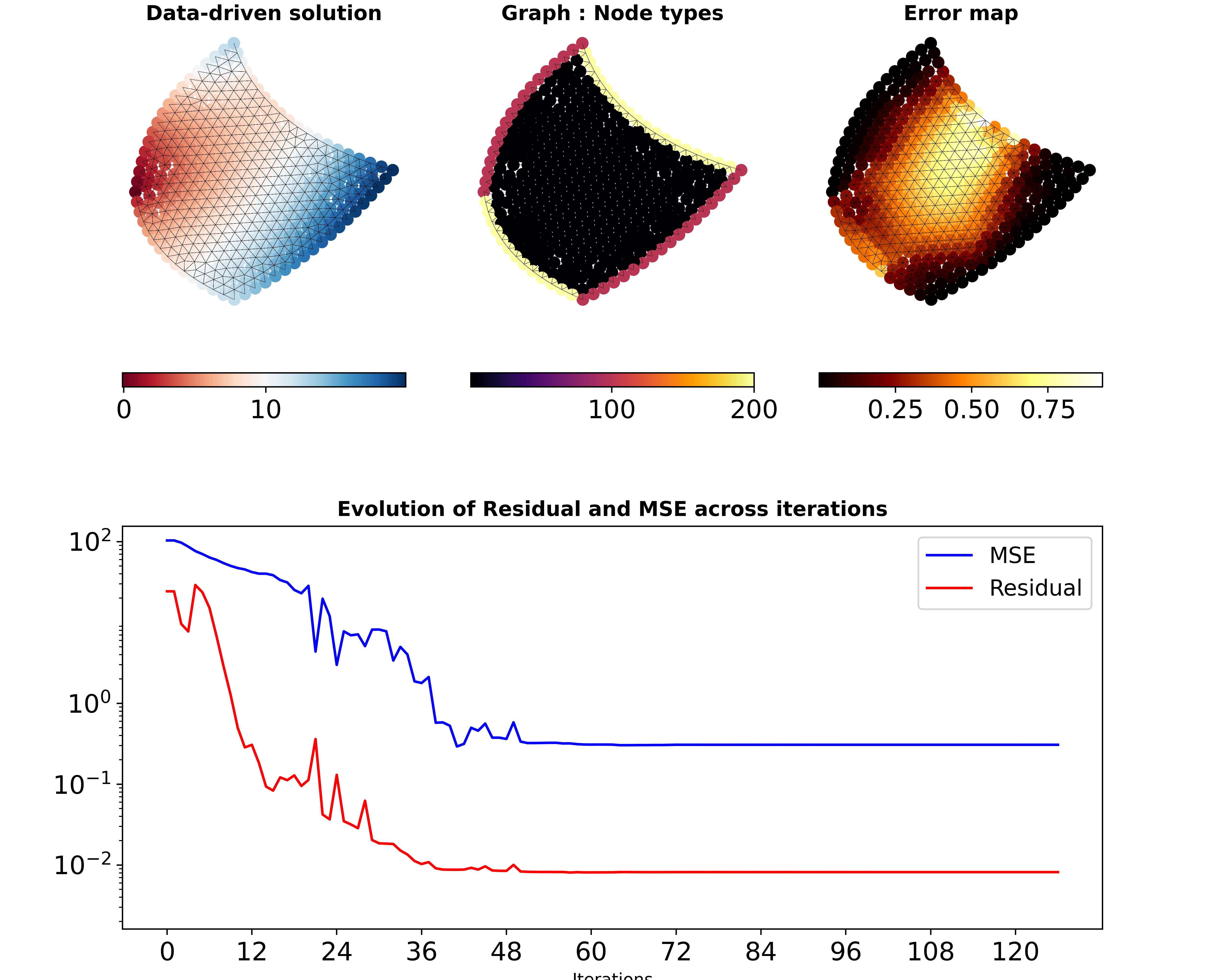
Figure 2: Comparison between $\Psi$-GNN (top left) and the LU “ground truth” on a test example with $370$ nodes. At convergence: Residual loss: 8.17e-3, MSE loss: 3.07e-1, MSE for Dirichlet nodes: 3.27e-4. The top middle plot displays the three types of nodes (black: Interior, pink: Dirichlet, yellow: Neumann), and the top right plot shows the map of squared error. Bottom: evolution of the Residual and MSE loss along the $120$ iterations of the Broyden solver.

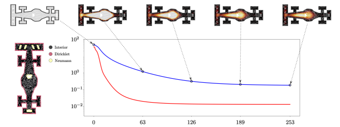
Figure 3: Generalization on the “out-of-distribution” F1 shape, 1219 nodes. Central plot: Residual and MSE during the 253 iterations of the Processor (i.e., without using RootFind), demonstrating the contractivity of $h_{\theta}$. Final values: Residual: 1.3e-2, MSE: 1.8e-1, MSE on Dirichlet nodes: 2.3e-4 and Spectral radius of the Jacobian: 0.97 are identical to those obtained when using RootFind. Left: The boundary conditions. Top: the visual evolution of the squared error, displaying the flow of information from Dirichlet nodes inward.

Contractivity  The purpose of the regularization term (23) is to constrain the spectral radius of the Jacobian $J_{h_{\theta}}(H^{*})$, ensuring the stability of the model around the fixed point $H^{*}$, as discussed in Section 3.4. The results on the test set indicate that this regularization is effective, with an average spectral radius of 0.989 $\pm$ 6e-4 $<$ 1, estimated a posteriori via the Power Iteration method (Golub & Van der Vorst, 2000). The regularization effect on the training process can be seen in Appendix E.1, where we observe the spectral radius converging towards $1$ as training progresses.

Out-of-distribution sample  To further illustrate this, we conduct an experiment on a geometry representing a caricatural Formula 1 with 1219 nodes. This geometry includes “holes” (such as a cockpit and front and rear wing stripes) and is larger (1219 nodes) than those seen in the training dataset, providing a challenging test of the model’s ability to generalize to out-of-distribution examples. We impose Dirichlet boundary conditions on all exterior nodes (pink nodes in the vertical plot at the left of Figure 3) and Neumann conditions on the nodes within the “holes” (yellow nodes). Functions $f$ and $g$ of (1) are randomly sampled from the same distribution as for the training set. The equilibrium of the model is found by simply iterating on the Processor instead of relying on Broyden’s algorithm. The stopping criteria is the relative error set to $10^{-5}$. The results Figure 3 demonstrate the contracting nature of the learned function that converges to the fixed point when iterated. Furthermore, it also demonstrates the generalization capacity of the learned model to this out-of-distribution example. Additionally, the figure also illustrates how the information propagates through the graph, starting from the Dirichlet nodes to gradually filling the whole domain.

Generalization analysis  In Appendix E, we present three supplementary experiments that assess the performance of $\Psi$-GNN on larger mesh sizes, initial solutions, and RootFind solvers. Firstly, we demonstrate in E.2 that the model can generalize effectively to larger dimensional geometries with similar low Residual loss values. However, we note relatively high MSE values, which may be attributed to increased problem conditioning. A future research direction is to investigate how to improve the conditioning of these problems in order to enhance performance. Secondly, in E.3, we demonstrate that $\Psi$-GNN can adapt the number of iterations required to reach convergence based on the proximity of the initial solution to the final solution. This ability allows $\Psi$-GNN to converge more efficiently by requiring fewer iterations if the initial solution is closer to the final solution. Finally, we show in E.4 that our model can achieve similar solutions using various RootFind solvers, such as the Broyden algorithm, Iteration on the Processor, or the Anderson acceleration solver (Walker & Ni, 2011). This demonstrates that $\Psi$-GNN is robust and flexible in its ability to adapt to different solvers.

Discussion  Comparing $\Psi$-GNN with other state-of-the-art Machine Learning models is not straightforward. The most similar work is that of Donon et al. (2020) (DSS), as previously discussed in Section 2. Although the problems addressed are different, as we now consider Neumann boundary conditions, the distinctions are noteworthy and are discussed in more detail in Appendix E.5. Specifically, we detail how we built upon the DSS architecture to create a general framework that is flexible to any mesh size and initial solution, and respects boundary conditions, making it more suitable for deployment in industrial context.

Inference Complexity  In order to determine the threshold at which performance enhancements can be expected, it is crucial to analyze the complexity of the model. By utilizing the forward iteration method, where the Processor is iterated upon, the complexity is found to be $\mathcal{O}(KNmd^{4})$, scaling linearly with the number of nodes, $N$. Here, $K$ represents the number of iterations, $d$ is the dimension of the latent space, and $m$ is the average size of the number of neighbours. On the other hand, when utilizing the Broyden method, the complexity corresponds to that of the Broyden algorithm, which is of $\mathcal{O}(MN^{2})$ if $M$ is the number of iterations of RootFind. $M$ being in general smaller than $K$ (though this remains to be proved), this complexity is somewhat lower than, for instance, that of the LU decomposition methods of complexity $\mathcal{O}(N^{3})$.

6 Conclusions and Future Work

This paper has introduced $\Psi$-GNN, a groundbreaking consistent Machine Learning-based approach that combines Graph Neural Networks and Implicit Layer Theory to effectively solve a wide range of Poisson problems. The model, trained in a “physics-informed” manner, is found to be robust, stable, and highly adaptable to varying mesh sizes, domain shapes, boundary conditions, and initialization, though more systematic experiments will explore and delineate its generalization capabilities. To the best of our knowledge, this approach is distinct from any previous Machine Learning based methods. Furthermore, $\Psi$-GNN can be extended to other steady-state partial differential equations and its application to 3-dimensional domains is straightforward. Overall, the results of this study demonstrate the significant potential of $\Psi$-GNN in solving Poisson problems in a consistent and efficient manner.

The long-term objective of the program driving this work is to accelerate industrial Computation Fluid Dynamics (CFD) codes on software platforms such as OpenFOAM (Chen et al., 2014). In future work, we aim to evaluate the efficiency of the proposed approach by implementing it in an industrial CFD code, and assessing its impact on performance acceleration. Moreover, despite its flexibility, the proposed method is still limited by the size of the graph. Therefore, scaling up using domain decomposition algorithms is being considered as a future direction.

Appendix A Architectural precision

This Appendix provides additional illustrations that describe the architectural elements mentioned in Section 3.2 and 3.3.

Particular shape of the graph  The structure of matrix A encodes the geometry of the corresponding mesh, as outlined in 3.2. Enforcing Dirichlet boundary conditions breaks the symmetry of matrix A, making the adjacency matrix a directed graph at the Dirichlet nodes. This means information is only sent to neighbours, not received, consistent with the definition of Dirichlet boundary conditions. Interior and Neumann nodes have bi-directional edges, allowing for information exchange until convergence. It’s important to note that although the graph is undirected at Interior and Neumann nodes, their stencils in matrix A are different, motivating separate Message Passing in the architecture 3.3. Figure 4 illustrates such a graph with the three types of nodes: Interior, Dirichlet and Neumann.

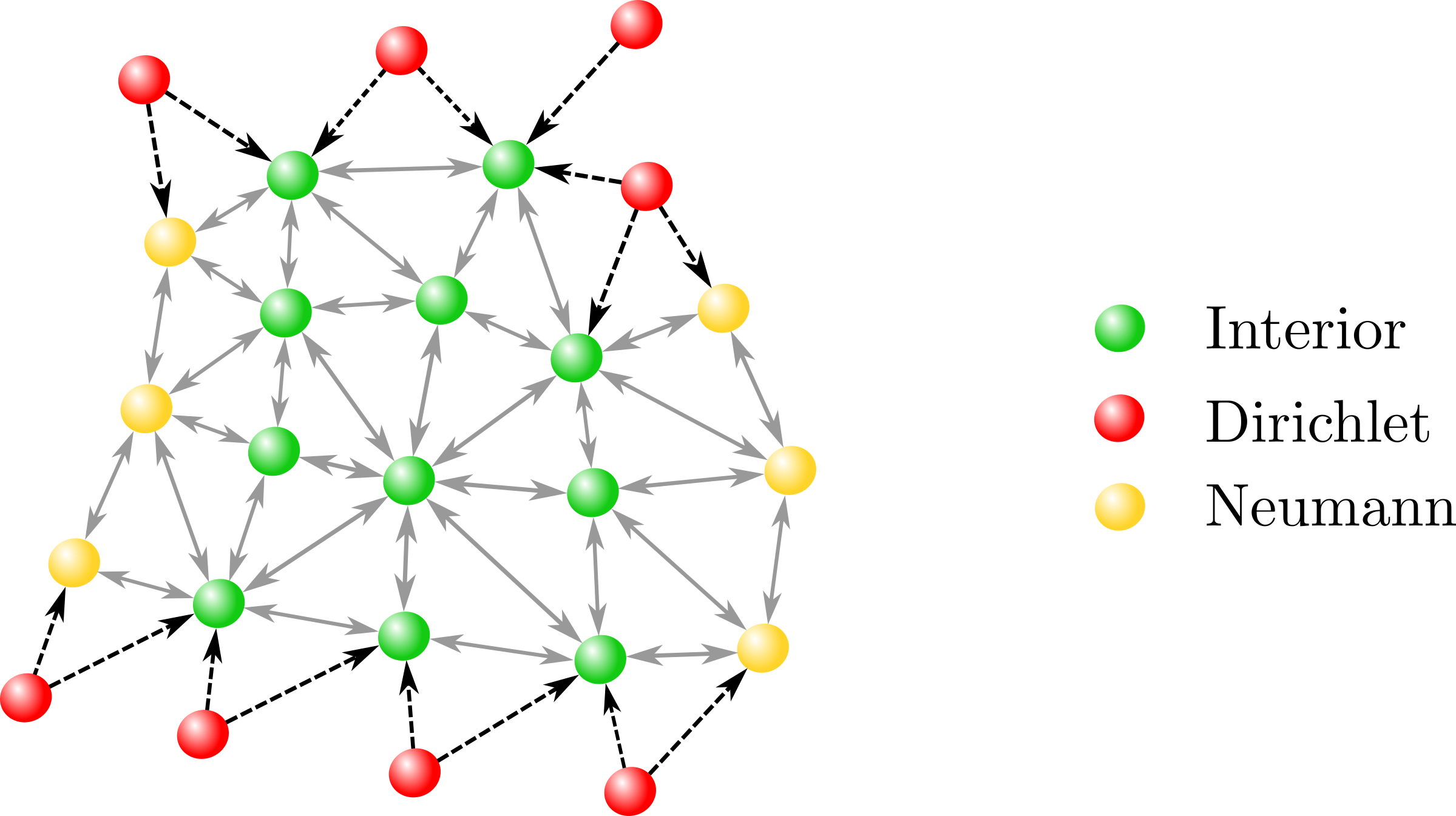
Figure 4: Sketch of a considered graph, which includes the three types of nodes: Interior (green), Dirichlet (red), and Neumann (yellow). The graph is directed at the Dirichlet nodes (dashed black arrows) and bi-directional between Neumann and Interior nodes (solid grey arrows).

Interior nodes messages  Figure 5 illustrates the update of an Interior node $i$, as described in 3.3.

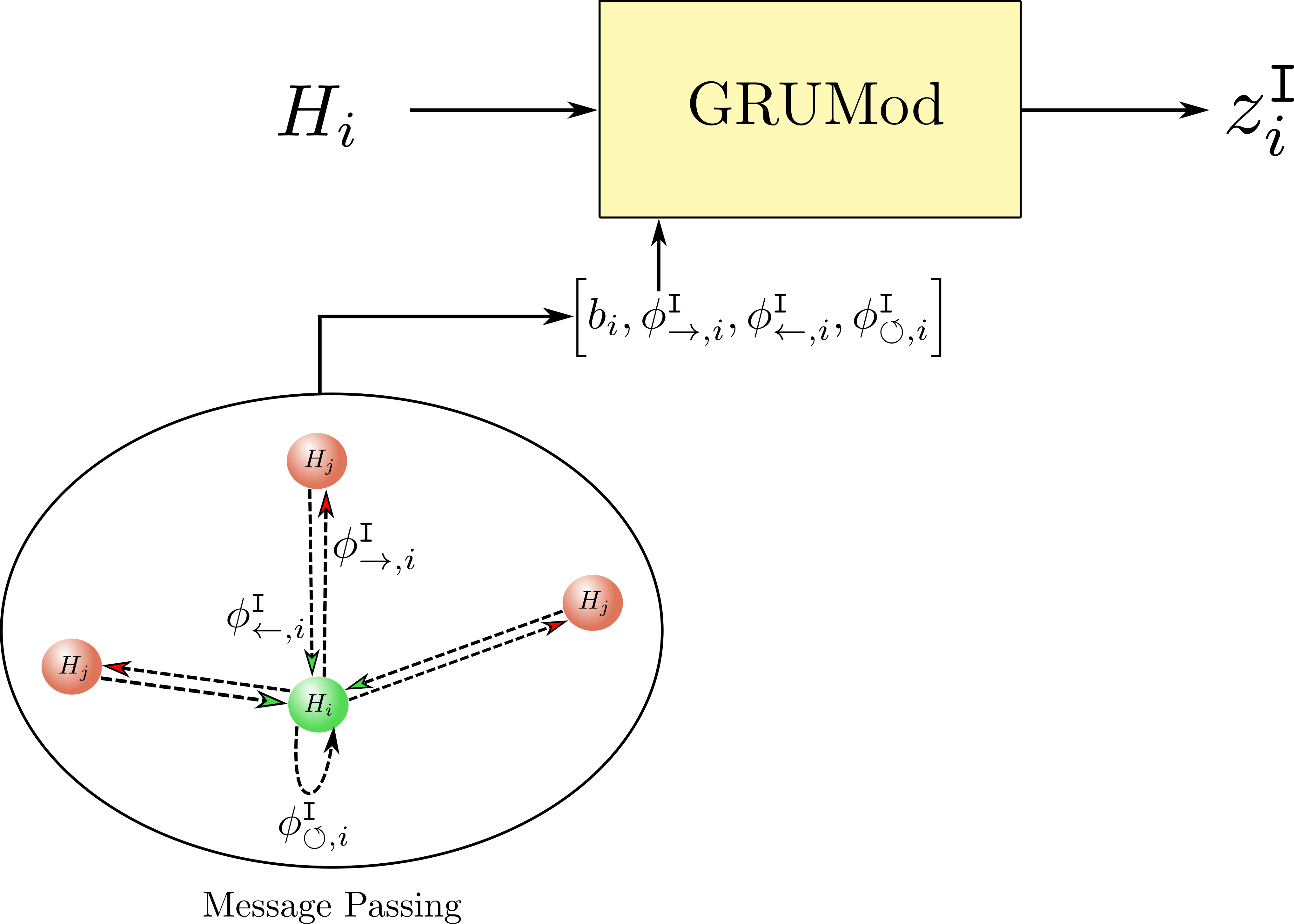
Figure 5: Update of an interior latent node $i$: First, incoming, outgoing, and self-loop messages ($\phi_{\leftarrow,i}^{\texttt{I}}$, $\phi_{\rightarrow,i}^{\texttt{I}}$, and $\phi_{\circlearrowleft,i}^{\texttt{I}}$) are computed (circled at the bottom). Next, these messages are combined with problem-specific data $b_{i}$ and passed as input to a modified GRU cell (GRUMod). The GRUMod uses the current latent state $H_{i}$ as latent input and outputs the updated latent state $z^{i}$.

Appendix B Supplementary materials for training

This Appendix provides additional training material, explaining the format of vectors considered in 3.3 and the normalization performed on the data.

Data information  The architecture of the model described in 3.3 relies on several inputs whose format needs to be precise. In equation 9, the self-loop message uses a one-hot $t_{i}$ vector to differentiate node types $i$ such that:

$$t_{i}=\left\{\begin{array}[]{r c l}\begin{bmatrix}[r]1&0&0\end{bmatrix}&&i\text{ is Interior}\\ \begin{bmatrix}[r]0&1&0\end{bmatrix}&&i\text{ is Dirichlet}\\ \begin{bmatrix}[r]0&0&1\end{bmatrix}&&i\text{ is Neumann}\end{array}\right.,$$ (26)

Similarly, equations 10, 11, 12 and 16 requires problem-related data, encoded into a vector $b_{i}$ such that:

$$b_{i}=\left\{\begin{array}[]{r c l}\begin{bmatrix}[r]f_{i}&0&0\end{bmatrix}&&i\text{ is Interior}\\ \begin{bmatrix}[r]0&g_{i}&0\end{bmatrix}&&i\text{ is Dirichlet}\\ \begin{bmatrix}[r]0&0&f_{i}\end{bmatrix}&&i\text{ is Neumann}\end{array}\right.$$ (27)

where $f_{i}$ and $g_{i}$ are the discretized values of the volumetric function $f$ and the Dirichlet boundary function $g$ from the Poisson problem (1).

Data normalization  In such problems, it is mandatory to normalize the input features to enhance the performance of the model in the training phase. The distances $d_{ij}$ in equations (8), (7), (14), the problem-related vector $b_{i}$ in equations (10), (11), (12) and (16) and the normal vector $n_{i}$ in equation (16) are all normalized by subtracting their mean and dividing by their standard deviation, computed on the entire dataset. Therefore, all inputs used for solution inference are normalized.

Appendix C Implicit Models

This section delves into the Implicit Layer Theory, providing supplementary information on its implementation. The motivations for its use are outlined in C.1, followed by a detailed description of the training procedures in C.2, emphasising backpropagation and exploiting Theorem 1 in (Bai et al., 2019). Furthermore, a comprehensive analysis of the Hutchinson method (Hutchinson, 1990) used to calculate the regularizing term as defined in reference 23 is presented in C.3.

C.1 Motivations

Many architectures are available for training Graph Neural Network (GNN) models, as demonstrated in Wu et al. (2020). In the context of this work, where we aim to solve a Poisson problem on unstructured meshes by directly minimizing the residual of the discretized equation, the number of layers required to achieve convergence should be proportional to the diameters of the meshes under consideration. Figure 6 illustrates the two common GNN architectures traditionally used for this purpose. On the left, the final solution $\widehat{H}$ is obtained after iterating on different Message Passing layers $M^{i}_{\theta}$, each with distinct weights. This architecture is employed in approaches such as Donon et al. (2020). On the right, the architecture is of recurrent type, where the final solution is obtained by iterating on the same neural network $M_{\theta}$. This architecture has the advantage of significantly reducing the size of the model, as employed in the work of Nastorg et al. (2022). In both methods, the number of Message Passing steps is fixed, limiting the model’s ability to generalize to different mesh sizes. However, using the recurrent architecture, it has been experimentally demonstrated that the model, trained with a sufficient number of iterations, tends towards a fixed point.

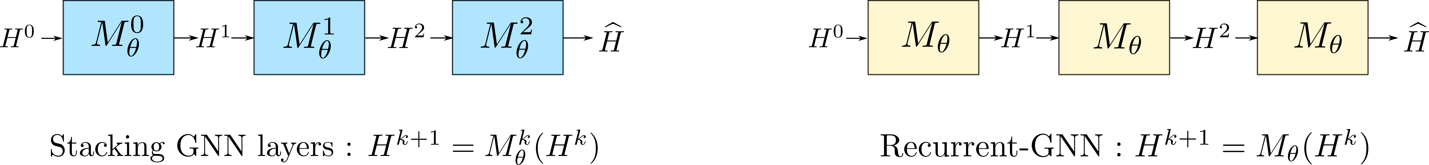
Figure 6: Comparison between a usual GNN architecture (left) where different Message Passing layers $M_{\theta}^{i}$ are stacked (i.e. the weights are different for all layers) and a Recurrent-GNN structure where the solution $\widehat{H}$ is computed iterating on the same Message Passing layer.

Building upon these previous experimental results, we propose to enhance the recurrent architecture by incorporating a black-box RootFind solver to directly find the equilibrium point of the model, as illustrated in figure 7. In this approach, the iterations (i.e. the flow of information) are performed implicitly within the RootFind solver. This method eliminates the need for a fixed number of iterations, as the number of required Message Passing steps is now exclusively determined by the precision imposed on the solver, resulting in a more adaptable and flexible approach.

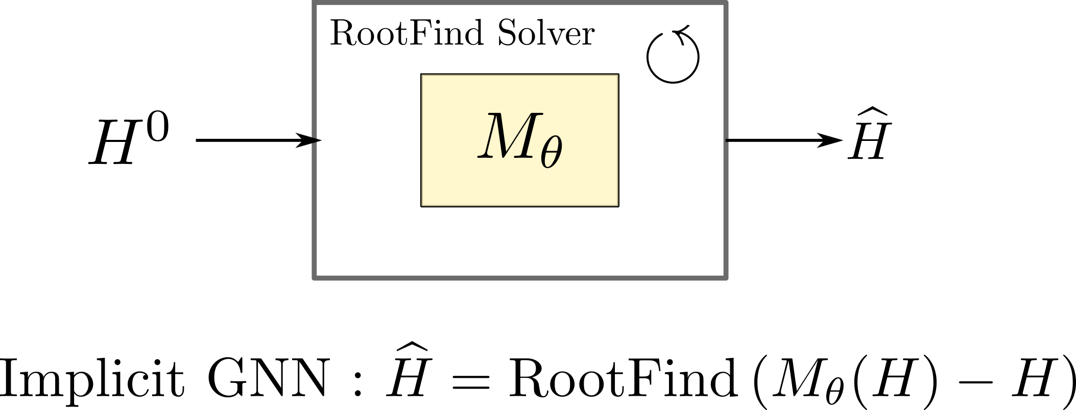
Figure 7: The figure illustrates the proposed implicit-GNN architecture. The final solution $\widehat{H}$ is computed as the equilibrium point of the $M_{\theta}$ function using a black-box RootFind solver. The solver is initialized with an initial condition $H^{0}$, and the Message Passing iterations are performed implicitly within the solver

C.2 Training an Implicit Model

Following Bai et al. (2019), the training of an implicit model requires, at each iteration, the resolution of two fixed point problems: one for the forward pass and one for the backward pass.

Forward pass  The resolution of a fixed point for the forward pass is clear and represents the core of our approach. A RootFind solver (i.e. a quasi-Newton method to avoid computing the inverse Jacobian of a Newton method at each iteration step) is used to determine the fixed point $H^{*}$ of the function $h_{\theta}$ (17) such that:

$$H^{*} =\text{RootFind}\left(h_{\theta}(H,G)-H\right)$$ (28)

Backward pass  However, using a black-box RootFind prevents the use of explicit backpropagation through the exact operations performed at inference. Thankfully, Bai et al. (2019) propose a simpler alternative procedure that requires no knowledge of the employed RootFind by directly computing the gradient at the equilibrium. The loss $\mathcal{L}$ with respect to the weights $\theta$ is then given by:

$$\frac{\partial\mathcal{L}}{\partial\theta}=-\frac{\partial\mathcal{L}}{\partial H^{*}}\left(J_{h_{\theta}}^{-1}|_{H^{*}}\right)\frac{\partial h_{\theta}(H^{*},G)}{\partial\theta}.$$ (29)

where $\left(J_{h_{\theta}}^{-1}|_{H^{*}}\right)$ is the inverse Jacobian of $h_{\theta}$ evaluated at $H^{*}$. To avoid computing the expensive $-\frac{\partial\mathcal{L}}{\partial H^{*}}\left(J_{h_{\theta}}^{-1}|_{H^{*}}\right)$ term in (29), one can alternatively solve the following root find problem using Broyden’s method (or any RootFind solver) and the autograd packages from Pytorch:

$$\left(J_{h_{\theta}}^{T}|_{H^{*}}\right)x^{T}+\left(\frac{\partial\mathcal{L}}{\partial H^{*}}\right)^{T}=0$$ (30)

Consequently, the model is trained using a RootFind solver to compute the linear system (30) and directly backpropagate through the equilibrium using (29).

C.3 Computing the regularizing term

In Section 3.4, we propose to rely on the method outlined in Bai et al. (2021) to regularize the model’s conditioning. The spectral radius of the Jacobian $\rho\left(J_{h_{\theta}}\right)$, responsible for the stability of the model around the fixed point $H^{*}$, is constrained by directly minimizing its Frobenius norm since it is an upper bound for the spectral radius. This method prevents the use of computationally expensive methods (i.e. Power Iteration (Golub & Van der Vorst, 2000) for instance). The Frobenius norm is estimated using the classical Hutchinson estimator ((Hutchinson, 1990)):

$$||J_{h_{\theta}}||^{2}_{F}=\mathbb{E}_{\epsilon\in\mathcal{N}(0,I_{d})}\left[||\epsilon^{T}J_{h_{\theta}}||^{2}_{2}\right]$$ (31)

where $J_{h_{\theta}}\in\mathbb{R}^{d\times d}$. The expectation (31) can be estimated using a Monte-Carlo method for which (empirically observed) a single sample suffices to work well.

Appendix D In-depth description of the dataset

This Appendix gives supplementary information on the dataset used in this study and described in 5. The dataset is diverse, consisting of a variety of sizes, shapes, force functions $f$, and Dirichlet boundary functions $g$ (from the Poisson problem (1)). It is inspired by the dataset used in Donon et al. (2020) and serves as a benchmark for evaluating the performance of our proposed method. Figure 8 illustrates three samples from the training set, along with their corresponding solutions, to give an idea of the complexity of the dataset.

Random domains  Random 2D domains $\Omega$ are generated using 10 points, randomly sampled in the unit square. These points are then connected using Bezier curves to form the boundary of the domain $\Omega_{h}$. We utilize the “MeshAdapt” mesher from GMSH (Geuzaine & Remacle, 2009) to discretize $\Omega$ into an unstructured triangular mesh $\Omega_{h}$. We randomly divide the geometry into fourths and apply Dirichlet boundary conditions on two opposite sections, while Neumann boundary conditions are imposed on the remaining opposite sections.

Random functions  Functions $f$ and $g$ are defined using the following equations:

$$f(x,y) =r_{1}(x-1)^{2}+r_{2}y^{2}+r_{3} (x,y) \in\Omega$$ (32)

$$g(x,y) =r_{4}x^{2}+r_{5}y^{2}+r_{6}xy+r_{7}x+r_{8}y+r_{9} (x,y) \in\partial\Omega$$ (33)

where $r_{i\in\left[1,\cdots,9\right]}$ are randomly sampled in $[-10,10]$.

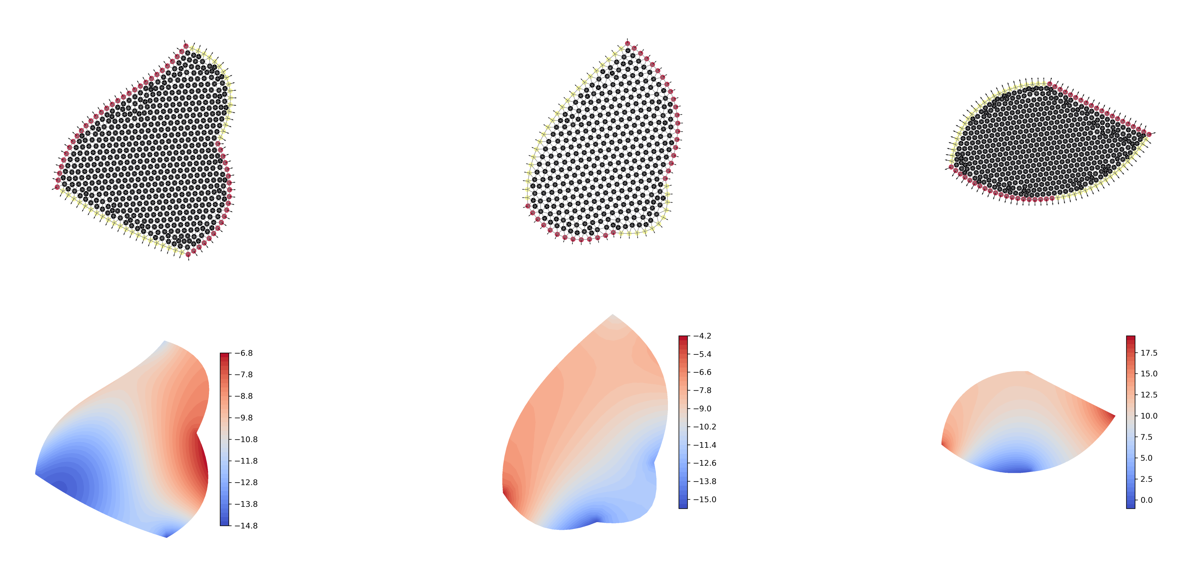
Figure 8: Example of three different domains extracted from the training set. Top: Discretized domains and their different node types (black: Interior, pink: Dirichlet, yellow: Neumann). The outward normal vectors are also displayed at the boundary of the domains. Bottom: The solution of a Poisson problem with random $f$ and $g$ functions applied to these geometries.

Appendix E Supplementary results

This Appendix provides additional information concerning the results highlighted in Section 5.

E.1 Spectral Radius evolution

Figure 9 displays the progression of the spectral radius throughout the training process, calculated at each epoch on the validation set utilizing the Power Iteration method (Golub & Van der Vorst, 2000). It illustrates the regularizing term’s impact, which aims to minimize the spectral radius, resulting in convergence towards a value of $1$.

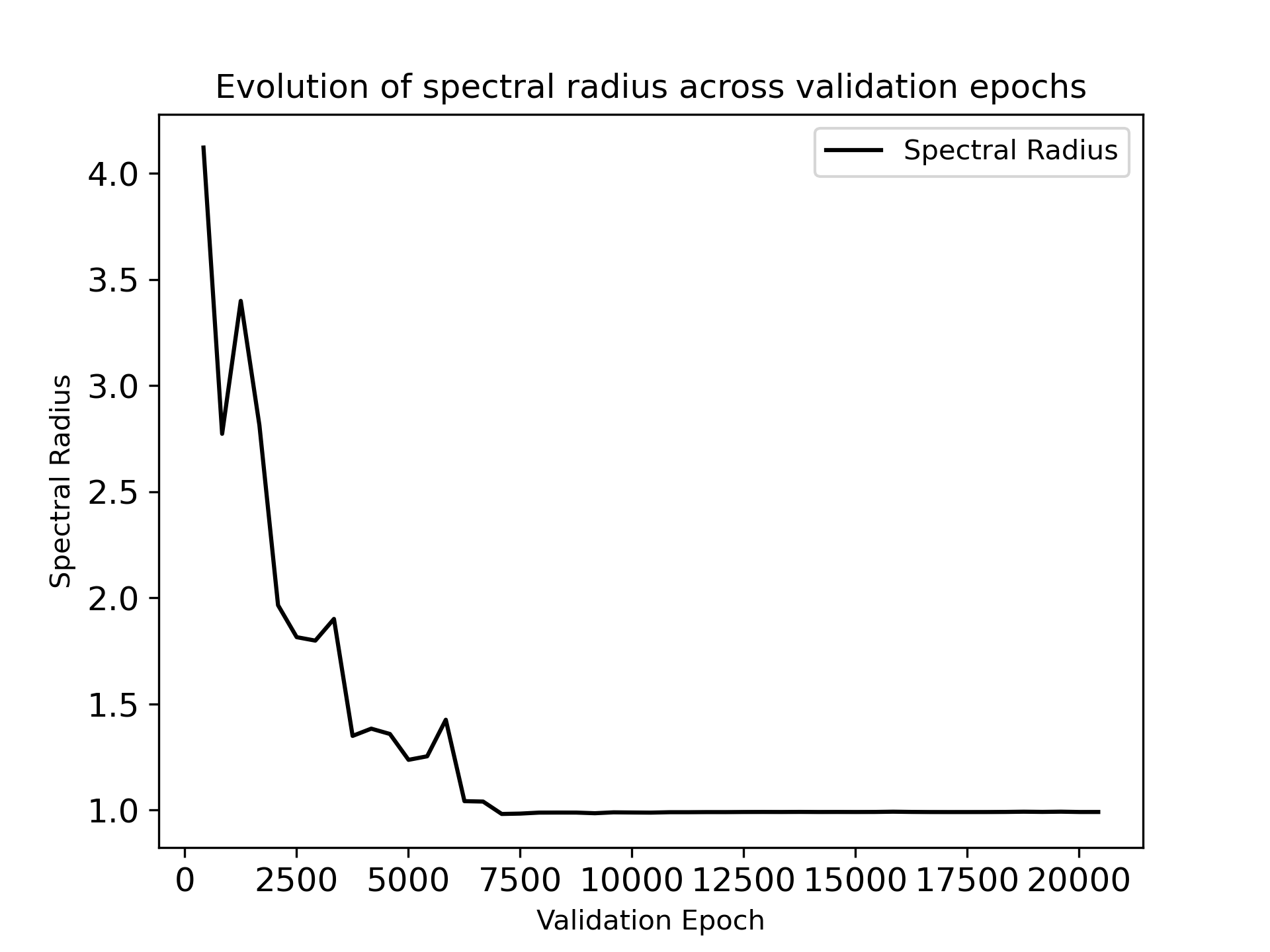
Figure 9: Evolution of spectral radius across the epochs of the validation set, converging towards a value of $1$ as the training progresses

E.2 Generalization analysis

In this section, we perform an in-depth study to evaluate the performance of $\Psi$-GNN when applied to higher-dimensional domains. To this end, we construct a new dataset, referred to as “LARGE,” following the methodology outlined in Sections 5 and D, which comprises domains with a range of nodes from 400 to 1000 (higher than the test dataset). Table 2 presents the results on the “LARGE” dataset and compares them with the results from the test set. The results indicate that $\Psi$-GNN is capable of effectively handling domains with a larger number of nodes, as evidenced by the similar low values of the Residual loss, indicating the versatility of our approach. However, we observe relatively high errors on the MSE, which may be attributed to increased problem conditioning. Specifically, the conditioning of the problem defined in (2), particularly when considering Neumann boundary conditions, increases with the size of the domains. Thus, investigating methods to improve the problem’s conditioning may be considered a potential avenue for future research to enhance the model’s generalization performance.

Table 2: Results averaged over the whole new “Large” dataset and the test set.

Metrics	Test	Large
Residual	1.25e-2 $\pm$ 1.3e-3	1.03e-2 $\pm$ 1.0e-2
MSE w/LU	9.17e-2 $\pm$ 2.6e-2	9.59 $\pm$ 3.48
Correlation w/LU	$>$ 99.9%	$>$ 92.1%

E.3 Various initializers

This section investigates the behaviour of $\Psi$-GNN when provided with different initial solutions. To achieve this, we conduct experiments on a consistent problem domain (in terms of mesh and functions) while considering three distinct initialization strategies. The first strategy, referred to as “train-like”, employs the standard initialization of our model, which is the assignment of zero values throughout the entire solution space. The second strategy is referred to as “far” and involves an initialization that is far from the exact solution by utilizing random uniform values between 50 and 1000. The third strategy, referred to as “close”, involves an initialization that is close to the final solution by slightly perturbing the “exact” LU solution with uniform noise taken from the interval [0,1]. The Dirichlet boundary nodes are set to their exact values for all these intializers, as required by the model. The tolerance for Broyden’s solver is fixed at $10^{-4}$ with a maximum number of 500 iterations. Figure 10 displays the evolution of the Residual loss for these three problems. The results demonstrate that $\Psi$-GNN is capable of convergence, regardless of the initial solution. Additionally, it illustrates the model’s superior autoencoding capabilities, as $\Psi$-GNN is able to understand, from the start, how close it is to the final solution and accordingly perform a variable number of iterations to reach convergence.

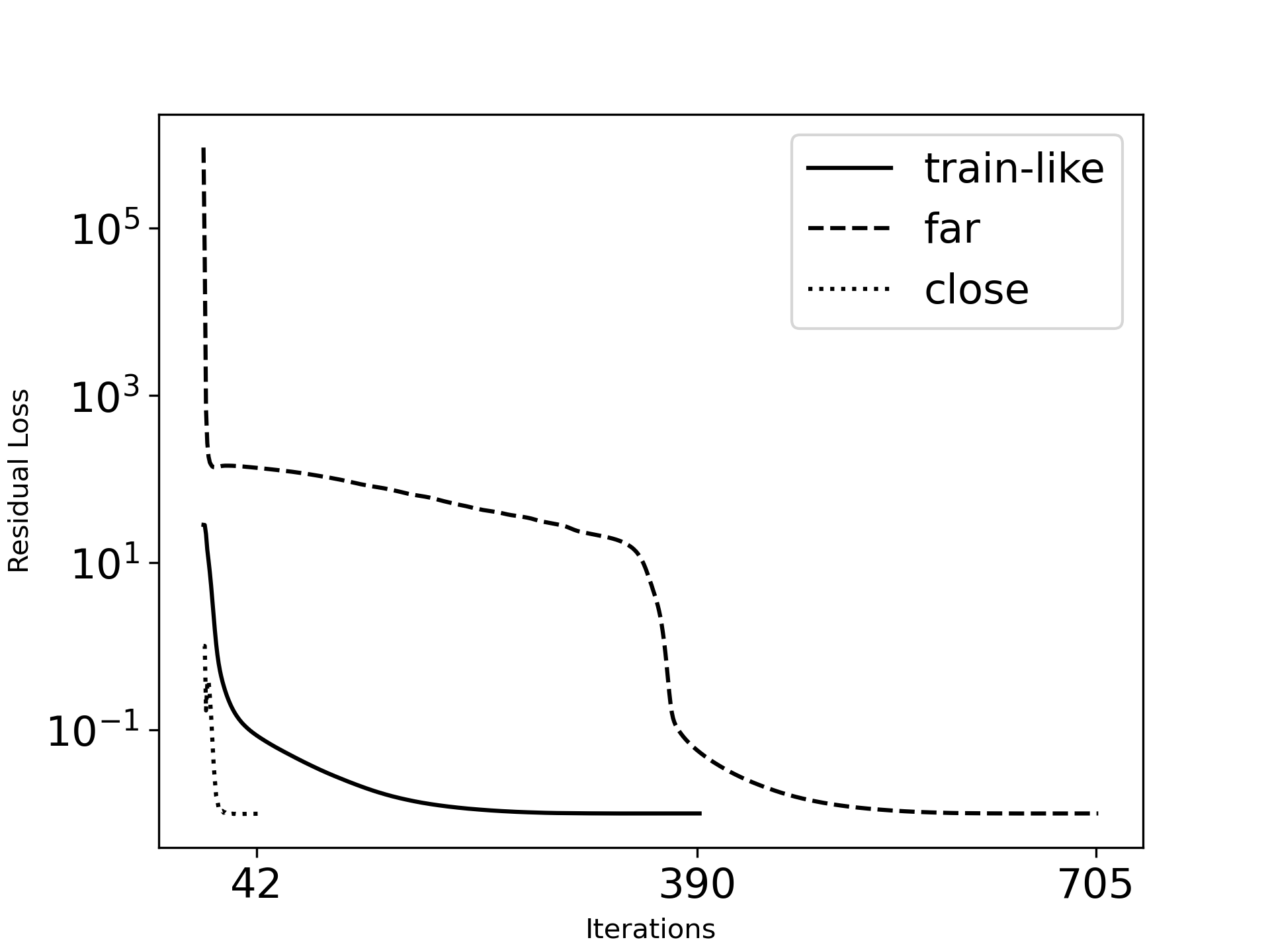
Figure 10: Evolution of the Residual loss for the three considered problems. As anticipated, the close initializer converges the quickest in 42 iterations, followed by the original one in 390 iterations, and finally, the far one in 705 iterations. This demonstrates that the proposed approach effectively converges towards the solution (for all problems!) accordingly with the distance from the initially provided solution to the final solution.

E.4 Various RootFind solvers

This section illustrates the flexibility of $\Psi$-GNN to converge towards its fixed point, regardless of the RootFind solver used. To demonstrate this, we evaluate the performance on the test set using three different RootFind solvers: the Broyden solver (the one utilized during training), the “Processor Iteration” (which exploits the contractivity nature of the built-in function $h_{\theta}$ defined in 17), and the Anderson acceleration solver (Walker & Ni, 2011). For all the solvers, the stopping criteria is the relative error, set to $10^{-5}$ with a maximum number of $500$ iterations. The results presented in Table 3 reveal extremely similar results, demonstrating the robustness of our model.

Table 3: Results averaged over the whole test set using different RootFind solvers

Metrics	Broyden	Forward	Anderson
Residual	1.25e-2 $\pm$ 1.e-3	1.25e-2 $\pm$ 1.3e-3	1.24e-2 $\pm$ 1.e-3
MSE w/LU	9.17e-2 $\pm$ 2.6e-2	1.1e-1 $\pm$ 3e-2	1.42e-1 $\pm$ 3.9e-2
Correlation w/LU	$>$ 99.9%	$>$ 99.9%	$>$ 99.9%

E.5 Discussion

It can be challenging to directly compare our proposed method, $\Psi$-GNN, and existing state-of-the-art Machine Learning models. The most closely related work is that of Donon et al. (2020) (DSS), as previously mentioned in Section 2. DSS employed a GNN-based model to solve a Poisson problem with Dirichlet boundary conditions. While the problems addressed are distinct, there are notable distinctions to highlight. Our approach incorporates Neumann boundary conditions, which renders the convergence of the problem more delicate. These specific boundary conditions indeed increase the condition number of the discretized Poisson operator $A$ in (2), making the residual equation (5) more difficult to minimize. $\Psi$-GNN extends upon the architecture of DSS by incorporating an autoencoding procedure, which makes the model adaptable to any initial condition, whereas DSS was initialized with a null latent space. Additionally, our method incorporates the proper treatment of boundary conditions, which is crucial in physical applications, as an inherent part of the network, unlike DSS. Furthermore, our model is based on the Theory of Implicit Layers, enabling the automatic propagation of information in the graph, thus adapting to different mesh sizes. In contrast, if DSS were applied to our dataset, it would require additional MPNN layers, resulting in a huge and untrainable model without considerable computational resources. Besides, even though previous research has explored the integration of GNNs with Implicit Layer Theory, such as the work of Gu et al. (2020) or Li et al. (2021), our approach is, to the best of our knowledge, the first attempt to apply it considering a physical-based function and a physical application in the context of solving partial differential equations.

Appendix F Theoretical proofs

Lemma F.1 (Equivalence of direct and fixed point formulations).

Problems (24) and (25) are equivalent, i.e. for any problem $G$, any solution $U^{*}_{G}$ of

$$U^{*}(G)=\operatorname*{argmin}_{U}\mathcal{L}_{\text{res}}(U,~{}G)$$

can be turned into a solution $h_{G}^{*}$ of

$$h_{G}^{*}=\operatorname*{argmin}_{h}\mathcal{L}_{\text{res}}(\text{FixedPoint}(h),~{}G)$$

and reciprocally.

Proof.

If $h_{G}^{*}$ is a solution of Problem (25), then its fixed point is a candidate solution to Problem (24). Therefore $\mathcal{L}_{\text{res}}(\text{FixedPoint}(h_{G}^{*}),~{}G)\geqslant\mathcal{L}_{\text{res}}(U^{*}_{G},~{}G)$.

Reciprocally, if $U^{*}_{G}$ is a solution of Problem (24), then the functional $h(H,G)=U^{*}_{G}$ which always outputs the same value has a unique fixed point, namely $U^{*}_{G}$. Considering this functional as a candidate for Problem (25), we get $\mathcal{L}_{\text{res}}(U_{G}^{*},~{}G)\geqslant\mathcal{L}_{\text{res}}(\text{FixedPoint}(h^{*}_{G}),~{}G)$.

Thus $\mathcal{L}_{\text{res}}(U_{G}^{*},~{}G)=\mathcal{L}_{\text{res}}(\text{FixedPoint}(h^{*}_{G}),~{}G)$ and the problems are equivalent. ∎

Proposition F.2 (Satisfying the conditions of DSS’s Corollary 1).

The conditions of Deep Statistical Solver’s Corollary 1 are satisfied in the case of our problem to approximate the function $\varphi:G=(N,A,B)\;\mapsto\;U^{*}(G):=\operatorname*{argmin}_{U}\mathcal{L}_{\text{res}}(U,~{}G)$.

The conditions of Deep Statistical Solver’s Corollary 1 (Donon et al., 2020) are:

• the loss $\mathcal{L}_{\text{res}}$ is continuous and permutation-invariant (w.r.t. node indexing)

• the solution $U^{*}_{G}$ is unique

• this solution is continuous w.r.t. $G$

• the distribution of problems $G$ satisfies:

  • permutation-invariance

  • compactness

  • connectivity (each graph has a single connected component)

  • separability of external outputs (identificability of nodes)

The first point is immediate given the type of loss we consider here (suited for graph-NN problems). Moreover the unicity of the solution is granted by design of the task (Section 3.1). The continuity of the solution $U^{*}_{G}$ w.r.t. $G$ depends on the precise loss $\mathcal{L}_{\text{res}}$ considered. For Poisson-like problems, the continuity holds indeed:

Lemma F.3 (Continuity of $\varphi$).

The mapping $\displaystyle\varphi:G=(N,A,B)\;\mapsto\;U^{*}(G):=\operatorname*{argmin}_{U}\mathcal{L}_{\text{res}}(U,~{}G)$ is continuous w.r.t. $A$ and $B$ in our case where $\mathcal{L}_{\text{res}}(U,~{}G)=\|AU-B\|^{2}$ and where $A$ is the graph Laplacian.

Proof.

Poisson problems have a unique solution which is $U^{*}(G)=(A^{T}A)^{\dagger}A^{T}B$ where ^† denotes the pseudo-inverse. This quantity is linear in $B$ and thus continuous w.r.t. $B$. On the other side, the pseudo-inverse functional is not continuous in general, but it is continuous within subspaces of same-rank matrices. When the coordinates of graph nodes move (little enough not to cross each other), the graph Laplacian matrix $A$ changes smoothly and keeps the same rank ($N-3$). The pseudo-inverse of $A$ is then locally continuous (within the set $\mathcal{A}$ of matrices $A$ that are graph Laplacians of some graph) and consequently $U^{*}(G)$ is continuous in $A\in\mathcal{A}$ as well. ∎

Concerning problem distribution properties, our dataset generator does satisfy by design the three first points (generate a smooth boundary within a given bounded domain, following a law that is rotation-equivariant and that makes sure that its inside has only one connected component, and then mesh it). Node identificability within a graph comes from its edge features denoting distances to closest neighbors, as they are never equal in practice (as for random float numbers). If one wishes to enforce identificability (always and not just almost surely), one can add as a descriptor to each node its location in space. Experiments have actually been run in that setting, with no observable difference in performance.

We thus obtain, by applying Deep Statistical Solver’s Corollary 1:

Corollary F.4 (Existence of a graph-NN approximating $\varphi$).

For any $\varepsilon>0$, there exists a graph-NN $\widehat{\varphi}$ such that for any problem $G$ from our problem distribution,

$$\|\widehat{\varphi}(G)-U^{*}_{G}\|\leqslant\varepsilon\;.$$

Hence, we can approximate with graph-NNs the functional $h^{*}(H,G):=\varphi(G)=U^{*}(G)$, which is optimal for our loss. Note that this functional is (extremely) contractive w.r.t. $H$ for fixed $G$, and that many other very different optimal functionals (yielding the same fixed point) exist.

As the set of solutions (in the space of functionals $h$) is large (though they all yield the same fixed point $U^{*}_{G}$), and that this set includes in particular the one above that is infinitely contractive, one can choose an optimal solution which in plus is contractive. This can be done, in a Lagrangian spirit, instead of a supplementary constraint, by adding a penalty to the loss, as done in Eq (23).

The graph-NN obtained by this Corollary is however not necessarily recurrent (layers may differ from each other) while our implicit-GNN construction requires that all layers are equal. Fortunately, DSS’s Corollary 1 proof can be adapated to fulfill this extra constraint, as follows. The graph-NN it builds consists of two particular single layers, followed by identical ones. Grouping layers in blocks of 2, we see that all blocks are identical except for the first one, leading to only 2 types of blocks. One can merge them into a single block that would express if (firsttime) then Block1 else Block2. This can be done by adding an extra descriptor to every input node, that is always 0. When this descriptor is 0, one applies Block1 and sets that descriptor to $1$. When the descriptor is $1$, one applied Block2 and let the descriptor set to $1$. The function thus described can be approximated by a few-layer graph-NN (potentially very easily with just 2 layers if using attention mechanisms). In all cases we obtain a single block that can be used to build an implicit-GNN. And thus we can adapt the corollary into:

Corollary F.5 (Existence of an implicit graph-NN whose fixed point approximates $\varphi$).

For any $\varepsilon>0$, there exists an implicit graph-NN $h$ such that for any problem $G$ from our problem distribution, the function $h(H,G)$ has a unique fixed point $H^{*}_{G}$ w.r.t. $H$, which satisfies:

$$\|H^{*}_{G}-U^{*}_{G}\|\leqslant\varepsilon\;.$$

Our architecture is such an implicit graph-NN, but surrounded by an auto-encoder, applied independently node by node to their features, with a larger latent space than input space. This auto-encoder could be chosen to be the identity on these features (completed by 0 on extra dimensions) and thus we now have:

Theorem F.6 (Universal Approximation Property).

For any arbitrary precision $\varepsilon>0$, considering sufficiently large layers, there exists a parameterization $\theta$ of our architecture which yields a function $h_{\theta}(H,G)$ which is “mainly” contractive w.r.t. $H$, and whose fixed point will be the optimal solution of our task (24) up to $\varepsilon$, given as input any problem $G$ with any mesh, boundary conditions and force terms.

Proof.

The only point that remains to be proven is that the function $h_{\theta}(H,G)$ can be assumed to be “mainly” contractive w.r.t. $H$ for a given problem $G$. More exactly, we will show that the function is contractive w.r.t. $H$ for any pair of points farther than $\varepsilon$, and that an iterative power method will reach, from any initialization $H$, a ball of radius $\varepsilon$ around the fixed point $H^{*}_{G}$.

The network $h$ from Corollary F.5 can be assumed to be an approximation of a contractive function $f$ (as explained above). Thus for any problem $G$, and any latent values $H$, $H^{\prime}$:

$$d(f(H),f(H^{\prime}))\;\leqslant\;\lambda\,d(H,H^{\prime})$$

for some contraction factor $\lambda\in[0,1[$ (that could be assumed to be even 0), and for the Euclidean metric $d$. Thus:

$$d(h(H),h(H^{\prime}))\;\leqslant\;d(f(H),f(H^{\prime}))+2\varepsilon\;\leqslant\;\lambda\,d(H,H^{\prime})+2\varepsilon$$

since $\|h(H)-f(H)\|\leqslant\varepsilon$ and $\|h(H^{\prime})-f(H^{\prime})\|\leqslant\varepsilon$. Let us define $\mu=\lambda+2\sqrt{\varepsilon}<1$ for some $\varepsilon$ small enough. Then, for $H,H^{\prime}$ not too close, i.e. satisfying $d(H,H^{\prime})>\sqrt{\varepsilon}$, we have:

$$d(h(H),h(H^{\prime}))\;\leqslant\;\mu\,d(H,H^{\prime})$$

as $\lambda\,d(H,H^{\prime})+2\varepsilon<\mu\,d(H,H^{\prime})$ is equivalent to $d(H,H^{\prime})>\frac{2\varepsilon}{\mu-\lambda}=\sqrt{\varepsilon}$.

Thus $h$ is contractive for all pairs of points farther than $\sqrt{\varepsilon}$ from each other. In particular, if $d(H,H^{*}_{G})>\sqrt{\varepsilon}$, then $d(h(H),h(H^{*}_{G}))\leqslant\mu\,d(H,H^{*}_{G})$, which implies the exponential convergence of an iterative power method from any initialization $H$ to the ball of radius $\sqrt{\varepsilon}$ around the fixed point $H^{*}_{G}$, which is itself at distance at most $\varepsilon$ from the true optimal solution $U^{*}_{G}$. Thus the function $h$ is “mainly” contractive in that sense. Using $\varepsilon^{\prime}=\varepsilon+\sqrt{\varepsilon}$ then gets rid of square roots.

∎

References

- Alet et al. (2019) Alet, F., Jeewajee, A. K., Villalonga, M. B., Rodriguez, A., Lozano-Perez, T., and Kaelbling, L. Graph element networks: adaptive, structured computation and memory. In International Conference on Machine Learning, pp. 212–222. PMLR, 2019.
- Ba et al. (2016) Ba, J. L., Kiros, J. R., and Hinton, G. E. Layer normalization. arXiv preprint arXiv:1607.06450, 2016.
- Bai et al. (2019) Bai, S., Kolter, J. Z., and Koltun, V. Deep equilibrium models. Advances in Neural Information Processing Systems, 32, 2019.
- Bai et al. (2021) Bai, S., Koltun, V., and Kolter, J. Z. Stabilizing equilibrium models by jacobian regularization. arXiv preprint arXiv:2106.14342, 2021.
- Battaglia et al. (2016) Battaglia, P., Pascanu, R., Lai, M., Jimenez Rezende, D., et al. Interaction networks for learning about objects, relations and physics. Advances in neural information processing systems, 29, 2016.
- Brandstetter et al. (2022) Brandstetter, J., Worrall, D., and Welling, M. Message passing neural pde solvers. arXiv preprint arXiv:2202.03376, 2022.
- Broyden (1965) Broyden, C. G. A class of methods for solving nonlinear simultaneous equations. Mathematics of computation, 19(92):577–593, 1965.
- Cai et al. (2022) Cai, S., Mao, Z., Wang, Z., Yin, M., and Karniadakis, G. E. Physics-informed neural networks (pinns) for fluid mechanics: A review. Acta Mechanica Sinica, pp. 1–12, 2022.
- Chen et al. (2014) Chen, G., Xiong, Q., Morris, P. J., Paterson, E. G., Sergeev, A., and Wang, Y. Openfoam for computational fluid dynamics. Notices of the AMS, 61(4):354–363, 2014.
- Chen et al. (2022) Chen, R., Jin, X., and Li, H. A machine learning based solver for pressure poisson equations. Theoretical and Applied Mechanics Letters, 12(5):100362, 2022.
- Cheng et al. (2021) Cheng, L., Illarramendi, E. A., Bogopolsky, G., Bauerheim, M., and Cuenot, B. Using neural networks to solve the 2d poisson equation for electric field computation in plasma fluid simulations. arXiv preprint arXiv:2109.13076, 2021.
- Chung et al. (2014) Chung, J., Gulcehre, C., Cho, K., and Bengio, Y. Empirical evaluation of gated recurrent neural networks on sequence modeling. arXiv preprint arXiv:1412.3555, 2014.
- Donon et al. (2020) Donon, B., Liu, Z., Liu, W., Guyon, I., Marot, A., and Schoenauer, M. Deep statistical solvers. Advances in Neural Information Processing Systems, 33:7910–7921, 2020.
- Fey & Lenssen (2019) Fey, M. and Lenssen, J. E. Fast graph representation learning with pytorch geometric. arXiv preprint arXiv:1903.02428, 2019.
- Gao et al. (2022) Gao, H., Zahr, M. J., and Wang, J.-X. Physics-informed graph neural galerkin networks: A unified framework for solving pde-governed forward and inverse problems. Computer Methods in Applied Mechanics and Engineering, 390:114502, 2022.
- Geuzaine & Remacle (2009) Geuzaine, C. and Remacle, J.-F. Gmsh: A 3-d finite element mesh generator with built-in pre-and post-processing facilities. International journal for numerical methods in engineering, 79(11):1309–1331, 2009.
- Golub & Van der Vorst (2000) Golub, G. H. and Van der Vorst, H. A. Eigenvalue computation in the 20th century. Journal of Computational and Applied Mathematics, 123(1-2):35–65, 2000.
- Gu et al. (2020) Gu, F., Chang, H., Zhu, W., Sojoudi, S., and El Ghaoui, L. Implicit graph neural networks. Advances in Neural Information Processing Systems, 33:11984–11995, 2020.
- Guermond & Quartapelle (1998) Guermond, J.-L. and Quartapelle, L. On stability and convergence of projection methods based on pressure poisson equation. International Journal for Numerical Methods in Fluids, 26(9):1039–1053, 1998.
- Hsieh et al. (2019) Hsieh, J.-T., Zhao, S., Eismann, S., Mirabella, L., and Ermon, S. Learning neural pde solvers with convergence guarantees. arXiv preprint arXiv:1906.01200, 2019.
- Hutchinson (1990) Hutchinson, M. F. A stochastic estimator of the trace of the influence matrix for laplacian smoothing splines. Communications in Statistics-Simulation and Computation, 19(2):433–450, 1990.
- Jin et al. (2021) Jin, X., Cai, S., Li, H., and Karniadakis, G. E. Nsfnets (navier-stokes flow nets): Physics-informed neural networks for the incompressible navier-stokes equations. Journal of Computational Physics, 426:109951, 2021.
- Kazhdan et al. (2006) Kazhdan, M., Bolitho, M., and Hoppe, H. Poisson surface reconstruction. In Proceedings of the fourth Eurographics symposium on Geometry processing, volume 7, 2006.
- Kochkov et al. (2021) Kochkov, D., Smith, J. A., Alieva, A., Wang, Q., Brenner, M. P., and Hoyer, S. Machine learning–accelerated computational fluid dynamics. Proceedings of the National Academy of Sciences, 118(21):e2101784118, 2021.
- Kumar & Yadav (2011) Kumar, M. and Yadav, N. Multilayer perceptrons and radial basis function neural network methods for the solution of differential equations: a survey. Computers & Mathematics with Applications, 62(10):3796–3811, 2011.
- Lagaris et al. (1998) Lagaris, I. E., Likas, A., and Fotiadis, D. I. Artificial neural networks for solving ordinary and partial differential equations. IEEE transactions on neural networks, 9(5):987–1000, 1998.
- Langtangen & Mardal (2019) Langtangen, H. P. and Mardal, K.-A. Introduction to Numerical Methods for Variational Problems. 01 2019. ISBN 978-3-030-23787-5. doi: 10.1007/978-3-030-23788-2.
- LeCun et al. (1995) LeCun, Y., Bengio, Y., et al. Convolutional networks for images, speech, and time series. The handbook of brain theory and neural networks, 3361(10):1995, 1995.
- Lee & Kang (1990) Lee, H. and Kang, I. S. Neural algorithm for solving differential equations. Journal of Computational Physics, 91(1):110–131, 1990.
- Li et al. (2021) Li, G., Müller, M., Ghanem, B., and Koltun, V. Training graph neural networks with 1000 layers. In International conference on machine learning, pp. 6437–6449. PMLR, 2021.
- Li et al. (2020) Li, Z., Kovachki, N., Azizzadenesheli, K., Liu, B., Bhattacharya, K., Stuart, A., and Anandkumar, A. Neural operator: Graph kernel network for partial differential equations. arXiv preprint arXiv:2003.03485, 2020.
- Luty et al. (1992) Luty, B. A., Davis, M. E., and McCammon, J. A. Solving the finite-difference non-linear poisson–boltzmann equation. Journal of computational chemistry, 13(9):1114–1118, 1992.
- Mannheim & Kazanas (1994) Mannheim, P. D. and Kazanas, D. Newtonian limit of conformal gravity and the lack of necessity of the second order poisson equation. General Relativity and Gravitation, 26(4):337–361, 1994.
- Morton & Mayers (2005) Morton, K. and Mayers, D. Numerical Solution of Partial Differential Equations: An Introduction. Cambridge University Press, 2005. ISBN 9781139443203. URL https://books.google.fr/books?id=0uf_iQIBFKgC.
- Nastorg et al. (2022) Nastorg, M., Schoenauer, M., Charpiat, G., Faney, T., Gratien, J.-M., and Bucci, M.-A. Ds-gps: A deep statistical graph poisson solver (for faster cfd simulations). arXiv preprint arXiv:2211.11763, 2022.
- Olver (2013) Olver, P. Introduction to Partial Differential Equations. Undergraduate Texts in Mathematics. Springer International Publishing, 2013. ISBN 9783319020990. URL https://books.google.fr/books?id=aQ8JAgAAQBAJ.
- Özbay et al. (2021) Özbay, A. G., Hamzehloo, A., Laizet, S., Tzirakis, P., Rizos, G., and Schuller, B. Poisson cnn: Convolutional neural networks for the solution of the poisson equation on a cartesian mesh. Data-Centric Engineering, 2, 2021.
- Raissi & Karniadakis (2018) Raissi, M. and Karniadakis, G. E. Hidden physics models: Machine learning of nonlinear partial differential equations. Journal of Computational Physics, 357:125–141, 2018.
- Reddy (2019) Reddy, J. N. Introduction to the finite element method. McGraw-Hill Education, 2019.
- Saad (2003) Saad, Y. Iterative methods for sparse linear systems. SIAM, 2003.
- Smaoui & Al-Enezi (2004) Smaoui, N. and Al-Enezi, S. Modelling the dynamics of nonlinear partial differential equations using neural networks. Journal of Computational and Applied Mathematics, 170(1):27–58, 2004.
- Tang et al. (2017) Tang, W., Shan, T., Dang, X., Li, M., Yang, F., Xu, S., and Wu, J. Study on a poisson’s equation solver based on deep learning technique. In 2017 IEEE Electrical Design of Advanced Packaging and Systems Symposium (EDAPS), pp. 1–3. IEEE, 2017.
- Um et al. (2020) Um, K., Brand, R., Fei, Y. R., Holl, P., and Thuerey, N. Solver-in-the-loop: Learning from differentiable physics to interact with iterative pde-solvers. Advances in Neural Information Processing Systems, 33:6111–6122, 2020.
- Walker & Ni (2011) Walker, H. F. and Ni, P. Anderson acceleration for fixed-point iterations. SIAM Journal on Numerical Analysis, 49(4):1715–1735, 2011.
- Wiewel et al. (2019) Wiewel, S., Becher, M., and Thuerey, N. Latent space physics: Towards learning the temporal evolution of fluid flow. In Computer graphics forum, volume 38, pp. 71–82. Wiley Online Library, 2019.
- Wu et al. (2018) Wu, J.-L., Xiao, H., and Paterson, E. Physics-informed machine learning approach for augmenting turbulence models: A comprehensive framework. Physical Review Fluids, 3(7):074602, 2018.
- Wu et al. (2020) Wu, Z., Pan, S., Chen, F., Long, G., Zhang, C., and Philip, S. Y. A comprehensive survey on graph neural networks. IEEE transactions on neural networks and learning systems, 32(1):4–24, 2020.