Abstract

Prostatectomized patients are at risk of resurgence: this is the reason why, during a follow-up period, they are monitored for PSA growth, an indicator of tumor progression. The presence of tumors can be evaluated with an expensive exam, called PET-PSMA (Positron Emission Tomography with Prostate-Specific Membrane Antigen). But, to optimize the benefit/risk ratio, patients should be referred to this exam only when the evidence is strong. The aim is to estimate the optimal time to recommend the exam, based on patients’ history and collected data. We build a Hierarchical Bayesian model that describes, jointly, the PSA growth curve and the probability of a positive PET-PSMA. Our proposal is to process all information about the patient in order to give an informed estimate of the optimal time.

PSA resurgence, PET-PSMA, optimal time, Bayesian modeling, joint model.

1 Introduction

Prostate cancer is the most frequent neoplasm in men, with an incidence of around 7% among all new cancer cases (https://gco.iarc.fr/today/online-analysis-pie) and has therefore attracted a lot of interest in the last twenty years. Research focuses on very different topics, starting from the causes and the incidence of this tumor, modeling its growth and analyzing the effect of therapies, and finally analyzing the risk, the locations, and the time of biochemical relapse (BCR) and clinical recurrences. High levels of Serum Prostate-Specific Antigen (PSA) after primary treatments such as surgery or radiotherapy were identified in the literature to be significant indicators of tumor progression which happen at some locations different from the original one [1, 8, 7, 23, 13]. In particular, prostatectomized patients are at risk of developing BCR and metastasis, which is the reason why, during a follow-up period of several years, they are usually monitored for PSA recurrence [1, 8, 7, 23, 13].

Since 2016, PET-PSMA has been available, a nuclear medicine survey that is currently one of the most sensitive tests for the early detection of locations of disease, but also quite expensive and complex. For this reason, it is crucial to optimize the benefit/risk ratio: patients should be referred to a PET-PSMA exam in case of BCR. Nevertheless, a single high value of PSA may not be sufficient evidence; instead, the kinetics and in particular the PSA doubling time (PSA-DT) are usually monitored over time to control the PSA evolution. According to literature, [19] data a PSA-DT<6 months, together with a thorough clinical examination of the patient stage and conditions, should be used as an indication to perform a PET-PSMA exam. The estimation of the optimal time to perform such an examination is still an open problem hugely discussed in the literature. Some authors simply model the PSA evolution over time trying to link it to tumor progression [20, 12], distinguishing between patients with and without disease [4, 18], or accounting of the impact of aging on its evolution [15]. Other work mainly focuses on the PET examination [9] or on the correlation between PSA levels and PET results [16]. Finally, some researches link PSA kinetics and tumor recurrence [18], whereas other authors try to find out the optimal time of PET-PSMA [14] regardless of the kinetics of PSA.

Our work combines many aspects of all these papers into an overall joint model. In particular, we address the problem of estimating more precisely the evolution of the probability of a positive PET-PSMA, and consequently the optimal time to recommend such an exam in the case of BCR. The aim of the present study is to gain accuracy by basing decisions on the individual clinical and serological patient history and on an entire database of similar patients, built on clinical practice, rather than relying solely on the last two individual measurements of PSA. To do so, a Bayesian Network (BN) [5] is built, or more precisely a Bayesian Hierarchical Model, which processes all information on the patient, and merges it to the observational database and gives an estimate of the optimal PET-PSMA time together with its associated uncertainty quantification. BNs are Probabilistic Graphical Models which represent a set of variables and their probabilistic interdependencies, allowing for the data analyst to update uncertainty quantification about them. Such an inferential operation is performed according to Bayes’ rule and to the principles of Bayesian Statistics.

The paper is organized as follows. In Section 2 we present the model for the PSA measurements and test results. Section 3 is devoted to the definition and the estimation of the optimal time to perform a test. In Section 4 there are simulated examples while Section 5 contains the results of the model estimated on a group of patients from San Luigi Gonzaga hospital, in Turin, Italy. The paper ends with some conclusive remarks in Section 6

2 Joint modelling of PSA growth and PET-PSMA results

2.1 The data and its likelihood

Let $x_{i}(t)\in\mathbb{R}^{+}$ be the PSA level of the $i$-th patient at time $t$, where $t=0$ indicates the time the patient has had a prostatectomy (only operated patients are considered in this work) and $i=1,2,\ldots,m$, where $m$ is the total number of patients in the study. The recorded variable $y_{i}(t)$ is a noisy version of $x_{i}(t)$, and we assume

$$\log y_{i}(t)\sim N(\log x_{i}(t),\sigma_{i}^{2}).$$

The choice of the functional form of $x_{i}(t)$, i.e. how PSA levels depend on time and other covariates, is one of the two major components of the joint model, but before we discuss it, let us introduce the second component, which is the probability $\pi_{i}(t)$ for patient $i$ at time $t$ that, if a PET-PSMA is taken, the result will be positive. For each patient, the test outcome $z_{i}(t)\in\{0,1\}$ is assumed to be a sample from a Bernoulli distribution with a patient-specific probability changing over time, i.e.,

$$z_{i}(t)\sim\text{Ber}(\pi_{i}(t)).$$

In our model, we can not observe $x_{i}(t)$ and $\pi_{i}(t)$, but only $y_{i}(t)$ and $z_{i}(t)$ at specific time points, which can differ between patients. Moreover, we do not assume that the PSA measurements and the PET-PSMA test results are observed at the same time points. The variable $y_{i}(t)$ in the set of time points $\mathcal{T}_{y,i}$, while $z_{i}(t)$ is measured in $\mathcal{T}_{z,i}$, so that $\mathcal{T}_{i}=\mathcal{T}_{y,i}\cup\mathcal{T}_{z,i}$ is the set of points where we have a measure of one of the two variables. Let $\mathbf{y}_{i}^{o}=\{y_{i}(t)\}_{t\in\mathcal{T}_{y,i}}$, $\mathbf{x}_{i}^{o}=\{x_{i}(t)\}_{t\in\mathcal{T}_{y,i}}$ be the observed and latent PSA values over the time points in $\mathcal{T}_{y,i}$ and let $\mathbf{z}_{i}^{o}=\{y_{i}(t)\}_{t\in\mathcal{T}_{z,i}}$, $\boldsymbol{\pi}_{i}^{o}=\{{\pi}_{i}(t)\}_{t\in\mathcal{T}_{z,i}}$ be the test results and probabilities over $\mathcal{T}_{z,i}$. Conversely, using the superscript $u$ for "unobserved" (as opposed to the previous $o$ for "observed"), let $\mathbf{y}_{i}^{u}=\{y_{i}(t)\}_{t\in\mathcal{T}_{z,i}}$, $\mathbf{x}_{i}^{u}=\{x_{i}(t)\}_{t\in\mathcal{T}_{z,i}}$, $\mathbf{z}_{i}^{u}=\{y_{i}(t)\}_{t\in\mathcal{T}_{y,i}}$, $\boldsymbol{\pi}_{i}^{u}=\{{\pi}_{i}(t)\}_{t\in\mathcal{T}_{y,i}}$ the vectors of variables at the time points where the associated process is not measured, i.e., $(y_{i}(t),x_{i}(t))$ at time points $\mathcal{T}_{z,i}$ where the exams are taken, and $(z_{i}(t),\pi_{i}(t))$ at time points $\mathcal{T}_{y,i}$ where the PSA is measured, respectively.

High values of PSA are indicators of tumor progression and thus are associated with a high probability of positive PET-PSMA results. We will then assume that $\pi_{i}(t)$ is a function of $x_{i}(t)$, and use this relation to find the optimal PET-PSMA time: this is the central idea of this work, an instance of joint modeling often used in Statistics to model longitudinal data [18, 22]. It should be noted that we define the relation in terms of the true latent PSA levels $x_{i}(t)$, not the observed ones $y_{i}(t)$. To specify the model we have to define the joint density of the variables $(\log y_{i}(t),z_{i}(t))^{\prime}$ over $\mathcal{T}_{i}$, for both observed and missing data. Hence, the missing data are considered further parameters to be estimated during the model fitting, which is a common approach within the Bayesian framework. We factorized the joint density in the following way

$$f(\log\mathbf{y}^{u},\log\mathbf{y}^{o},\mathbf{z}^{u},\mathbf{z}^{o}|\log\mathbf{x}^{u},\log\mathbf{x}^{o},\boldsymbol{\pi}^{u},\boldsymbol{\pi}^{o},\boldsymbol{\theta})=$$ (1)

$$\prod_{t\in\mathcal{T}_{i}} f(\log y_{i}(t)|\log x_{i}(t),\boldsymbol{\theta})f(z_{i}(t)|\log x_{i}(t),\pi_{i}(t),\boldsymbol{\theta}),$$

where $f(\cdot)$ stands for a generic probability density function (to be identified by its arguments) and $\boldsymbol{\theta}$ is a vector of parameters. In Equation (1) we are assuming that $(\log y_{i}(t),z_{i}(t))$ are conditionally independent given the latent variables. In the next paragraphs we declare our proposals for $f(\log y_{i}(t)|\log x_{i}(t),\boldsymbol{\theta})$ and $f(z_{i}(t)|\log x_{i}(t),\pi_{i}(t),\boldsymbol{\theta})$.

2.2 Joint model for each patient

To model the time evolution of PSA levels, we will assume that it is composed of two phases, the first one, right after prostatectomy, where the PSA level is stationary or even decrease over time and the second one after time $\tau_{i}$, a change point which is patient-dependent, where it is assumed that the PSA increases. In addition, we will assume that PSA levels will reach a plateau after some time. For each patient, the time $\tau_{i}$, i.e., the change point, can be interpreted as the unknown time at which resurgence starts, which is a crucial ingredient of our model. To model $\log x_{i}(t)$, we assume a linear function with patient-specific intercept, $\lambda_{i}$, and slope, $-\mu_{i}$, where $\mu_{i}\in\mathbb{R}^{+}$, before the change point $\tau_{i}$, i.e.,

$$\log x_{i}(t)=\lambda_{i}-\mu_{i}t,$$ (2)

while for $t>\tau_{i}$, we model $\log x_{i}(\tau_{i})$ as a weighted mean of the value at the change-point and of the asymptotic value $a_{i}$ of $\log x_{i}(t)$:

$$\log x_{i}(t)=\log x_{i}(\tau_{i})e_{i}(t)+a_{i}(1-e_{i}(t)).$$ (3)

The weight function $e_{i}(t)$ is defined as

$$e_{i}(t)=\exp(-\gamma_{i}(t-\tau_{i})),$$ (4)

with $\gamma_{i}\in\mathbb{R}^{+}$, to ensure that $\log x_{i}(t)$ is continuous at the change point $\tau_{i}$ and it reaches the asymptotic value $a_{i}$ as $t\rightarrow\infty$. Hence, for $t>\tau_{i}$, $x_{i}(t)$ is a version of the log-Gompertz growth function [21] with rate $\gamma_{i}$. We assume non-negative $\mu_{i}$ and $\gamma_{i}$ to model the decreasing phase before $\tau_{i}$ and the increasing phase after it.

The second part of the joint model is instead focused on the binary PET-PSMA result

$$z_{i}(t)\sim\text{Ber}(\pi_{i}(t)),$$ (5)

and in particular on modelling the probability $\pi_{i}(t)$. To connect the probability $\pi_{i}(t)$ to the PSA levels we use a logistic regression model

$$\text{logit}\{\pi_{i}(t)\}=\beta_{0,i}+\beta_{1}\log x_{i}(t)+\beta_{2}t,$$ (6)

where the linear prediction has a patient-specific intercept and an extra term linear on time to model temporal trends that can not be explained by $\log x_{i}(t)$. We expect $\beta_{1}$ to be a positive since the larger the PSA, the larger the probability of a positive test. It is easy to see, from equation (6), that, if $\beta_{1}>0$, then $\pi_{i}(t)$ goes to zero as $x_{i}$ goes to zero:

$$\lim_{x_{i}(t)\to 0^{+}}\pi_{i}(t)=\lim_{x_{i}(t)\to 0^{+}}\frac{x_{i}^{\beta_{1}}(t)e^{\beta_{0,i}+\beta_{2}t}}{1+x_{i}^{\beta_{1}}(t)e^{\beta_{0,i}+\beta_{2}t}}=0.$$ (7)

All the unknown quantities in the model $(\lambda_{i},\mu_{i},a_{i},\gamma_{i},\tau_{i},\beta_{0,i},\beta_{1},\beta_{2},\sigma_{i}^{2})$, for $i=1,\dots,m$, make up the parameter vector $\boldsymbol{\theta}$.

2.3 Completing the model using random effects

Section 2.2 contains the individual description of each patient, but the $m$ patients are not totally unrelated to one another and they should not be considered independent. Rather, as it is usually done in such an applied context, the patients are considered exchangeable, since they are similar to one another and they all contribute to the global learning of the PSA evolution. A hierarchical model is obtained in this way by introducing random effects to model some of the components of our proposal. As it is usually done in such applied contexts, random effects are often introduced as a way to model dependence between observations and to increase the precision of the parameter estimates, hence defining a hierarchical model. More precisely, we assume that the model describing PSA evolution can be enriched by the following second-level distributions:

$$\log\mu_{i} \sim N(\psi_{i,\mu},w_{\mu}^{2}),$$ (8)

$$\log\gamma_{i} \sim N(\psi_{i,\gamma},w_{\gamma}^{2}),$$ (9)

$$a_{i} \sim N(\psi_{i,a},w_{a}^{2}),$$ (10)

$$\lambda_{i} \sim N(\psi_{i,\lambda},w_{\lambda}^{2}),$$ (11)

$$\sigma_{i}^{2} \sim IG(a_{i,\sigma^{2}},b_{i,\sigma^{2}}),$$ (12)

for $i=1,\ldots,m$, where $IG$ indicates the inverse gamma distribution with scale parameter $a_{i,\sigma^{2}}$ and shape parameter $b_{i,\sigma^{2}}$, and $\psi_{i,\chi}$ and $w_{\chi}^{2}$ are respectively mean and variance of the normal distributions, for $\chi\in\{\mu,\gamma,a,\lambda,\sigma^{2}\}$. The log transformations are used to ensure that the parameters are defined in the correct domain. In Equations (8) the means of the normal distributions are allowed to vary from patient to patient since there may exist covariates that affect them via a linear regression approach as follows,

$$\psi_{i,\chi}=\mathbf{C}_{i,\chi}\boldsymbol{\alpha}_{\chi},$$ (13)

for $i=1,\ldots,m$, where $\mathbf{C}_{i,\chi}$ is a patient-specific vector of covariates of dimension $p_{\chi}$ and $\boldsymbol{\alpha}_{\chi}$ is a vector of regressors. Finally, covariate information can also be added to the model of $\pi_{i}(t)$ by defining, in equation (6), the following random intercept,

$$\beta_{0,i}=\mathbf{C}_{i,\beta}\boldsymbol{\alpha}_{\beta}.$$ (14)

The random effects $(a_{i,\sigma^{2}},b_{i,\sigma^{2}},\psi_{i,\chi},w_{i,\chi}^{2})$, for $\chi\in\{\mu,\gamma,a,\lambda,\sigma^{2}\}$, as well as the hyperparameters $\boldsymbol{\alpha}_{\chi}$, $\chi\in\{\mu,\gamma,a,\lambda,\sigma^{2},\beta\}$ are all appended to the parameter vector $\boldsymbol{\theta}$.

The strategy to estimate the optimal time to perform the PET-PSMA test is described in the next section.

3 Estimating the optimal time

3.1 Defining and identifying the optimal time

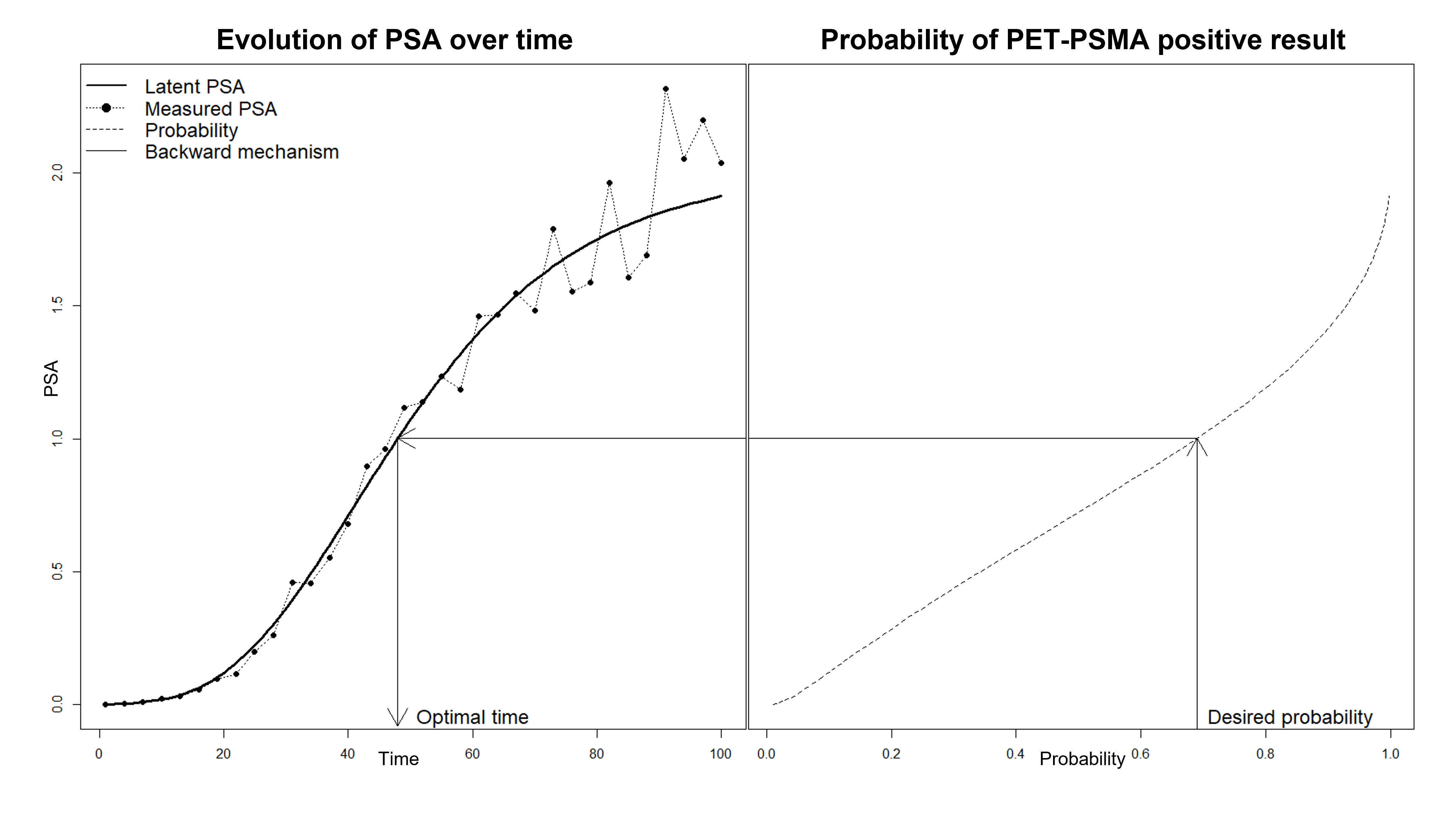
Figure 1: Joint modeling of $x_{i}(t)$ and $\pi_{i}(t)$. The plot shows the relation between time and PSA evolution, and between PSA and the probability of a positive test. After choosing the desired probability, the associated PSA and time can be recovered through the model, following the arrows.

Equation (7) gives a link between the probability of a positive PET-PSMA test and the unobserved PSA levels, which can be used to find the optimal time. One simple solution to find the optimal time could be to plug-in point estimates of all model parameters (maximum likelihood estimates, or Bayesian posterior means), and then invert equation (7) to target the desired probability. This strategy is viable, but it does not take into account all sources of uncertainty. The Bayesian approach, which we will follow globally to fit the model, gives a better way to estimate the optimal time and, simultaneously, account for uncertainty quantification in a controlled way.

In the Bayesian approach, the overarching goal is to compute the posterior density

$$f(\log\mathbf{y}^{u},\mathbf{z}^{u},\log\mathbf{x}^{u},\log\mathbf{x}^{o},\boldsymbol{\pi}^{u},\boldsymbol{\pi}^{o},\boldsymbol{\theta}|\log\mathbf{y}^{o},\mathbf{z}^{o}),$$ (15)

based on which all quantities of interest may be computed. Marginalizing the posterior density (15), one can easily obtain, for each fixed time point $t$, samples from the posterior predictive density

$$f(\pi_{i}(t),\tau_{i}|\log\mathbf{y}^{o},\mathbf{z}^{o});$$ (16)

it should be noted that this can be done since each specific $\tau_{i}$ is a component of the high dimensional parameter vector $\theta$ and, similarly, for each $t$, $\pi_{i}(t)$ is a parametric function. For each $t$, we can then verify whether the following condition is satisfied:

$$\mathcal{P}(\pi_{i}(t)>\pi^{*}\cap\,t>\tau|\log\mathbf{y}^{o},\mathbf{z}^{o})=\int_{\pi^{*}}^{1}\int_{0}^{t}f(\pi_{i}(t),\tau_{i}|\log\mathbf{y}^{o},\mathbf{z}^{o})d\tau_{i}d\pi_{i}(t)\geq\rho,$$ (17)

where:

• $\mathcal{P}$ stand for posterior predictive probability based on density (16);

• $\pi^{*}$ is a target probability of positive PET-PSMA;

• $\rho$ is a probability (say 95%), i.e. a posterior assurance probability, similar to a confidence coefficient.

Notice in Equation (17) we require $t$ to be greater than the change point $\tau_{i}$, and $\pi^{*}$ and $\rho$ are design parameters to be chosen in advance. Finally, to select the optimal time $t_{i}^{*}$ for the $i-$th patient, we can choose the first available time in the future satisfying (17), i.e. the smallest $t$ greater than the largest time in $\mathcal{T}_{i}$ satisfying (17). In Figure 1 we show a graphical depiction of the procedure used to obtain the optimal time and how the latent PSA level is connected to the probability of a positive test.

3.2 Computing the optimal time

The hierarchical joint model we have built is complicated and the posterior in equation (15), and in particular its normalizing constant, is difficult to compute given the high number of parameters. As often done, we use Markov Chain Monte Carlo (MCMC) [3] algorithms to obtain samples from (15) and to approximate the posterior quantities of interest, such as posterior expectations and posterior probabilities, with Monte Carlo integration[10]. Let then $\log\mathbf{y}^{u,b},\mathbf{z}^{u,b},\log\mathbf{x}^{u,b},\log\mathbf{x}^{o,b},\boldsymbol{\pi}^{u,b},\boldsymbol{\pi}^{o,b},\boldsymbol{\theta}^{b}$ be the $b$-th posterior samples from the associated parameters, where $b=1,2,\dots,B$ and $B$ is the number of MCMC iterations.

Using the posterior samples we can approximate the optimal-time $t_{i}^{*}$, since samples from the predictive distribution (16) are easily obtainable, as explained in the following. From equation (2), (3) and (6) we can see that $\pi_{i}(t)$, for all $t$, is a deterministic function of the parameters, even if $t$ is not in $\mathcal{T}_{i}$. Therefore, for a given $t$, and each $b$ sample, we can compute

$$\log x_{i}^{b}(t)=\begin{cases}\lambda_{i}^{b}-\mu_{i}^{b}t&\text{ if }t<\tau_{i}^{b}\\ \log x_{i}^{b}(\tau_{i}^{b})\exp(-\gamma_{i}^{b}(t-\tau_{i}^{b}))+a_{i}(1-\exp(-\gamma_{i}^{b}(t-\tau_{i}^{b})))&\text{ otherwise }\end{cases}$$ (18)

and

$$\pi_{i}^{b}(t)=\frac{\left(x_{i}^{b}(t)\right)^{\beta_{1}^{b}}e^{\beta_{0,i}^{b}+\beta_{2}^{b}t}}{1+\left(x_{i}^{b}(t)\right)^{\beta_{1}^{b}}e^{\beta_{0,i}^{b}+\beta_{2}^{b}t}},$$ (19)

and the set of samples $\{\pi_{i}^{b}(t),\tau_{i}^{b}\}_{b=1}^{B}$ are samples from the predictive distribution (16) . It is easy to see that the integral in (17) is an expectation if we rewrite it as

$$\int_{\pi^{*}}^{1}\int_{0}^{t}f(\pi_{i}(t),\tau_{i}|\log\mathbf{y}^{o},\mathbf{z}^{o})d\tau_{i}d\pi_{i}(t)=\int_{0}^{1}\int_{0}^{\infty}1_{[\pi^{*},1]}(\pi_{i}(t))1_{[0,t)}(\tau_{i})f(\pi(t),\tau_{i}|\log\mathbf{y}^{o},\mathbf{z}^{o})d\tau_{i}d\pi_{i}(t),$$ (20)

where $1_{\cdot}(\cdot)$ is the characteristic function of a set. Hence, using the samples from the predictive distribution, we can approximate the expectation using Monte Carlo integration, leading to

$$\int_{0}^{1}\int_{0}^{\infty}1_{[\pi^{*},1]}(\pi_{i}(t))1_{[0,t)}(\tau_{i})f(\pi(t),\tau_{i}|\log\mathbf{y}^{o},\mathbf{z}^{o})d\tau_{i}d\pi_{i}(t)\approx\frac{\sum_{b=1}^{B}1_{[\pi^{*},1]}(\pi_{i}^{b}(t))1_{[0,t)}(\tau_{i}^{b})}{B}.$$ (21)

This means that the integral can be approximated by the proportion of posterior samples that are in the space $[\pi_{i}(t)>\pi^{*},\tau_{i}<t]$. The approximation (21) must be computed for a fine grid of time points and the first $t\geq\max(\mathcal{T}_{i})$ that satisfies

$$\frac{\sum_{b=1}^{B}1_{[\pi^{*},1]}(\pi_{i}^{b}(t))1_{[0,t)}(\tau_{i}^{b})}{B}\geq\rho$$ (22)

is the estimated optimal time.

4 Simulations

Table 1: Simulated dataset - Results on individual parameters.

Parameter	Percentage dataset 1
$\log(\lambda_{i})$	93.75%
$\tau_{i}$	91.25%
$\log(\mu_{i})$	93.75%
$\log(\gamma_{i})$	95%
$\log(a_{i})$	100%
$\sigma^{2}_{i}$	93.75%

Table 2: Simulated dataset - Results global parameters.

Parameter	2.5%	Mean	97.5%	Real	Parameter	2.5%	Mean	97.5%	Real
$\alpha_{\mu}[1]$	0.95	1.05	1.14	1	$\alpha_{\beta}[1]$	-14.13	1.74	17.49	1
$\alpha_{\mu}$[2]	0.00	0.07	0.14	0.1	$\alpha_{\beta}[2]$	-5.11	0.65	5.65	1
$\alpha_{\mu}$[3]	0.19	0.26	0.34	0.3	$\alpha_{\beta}[3]$	-5.70	-0.25	5.62	1
$\alpha_{\mu}$[4]	0.38	0.45	0.53	0.5	$\alpha_{\beta}[4]$	-1.94	2.46	7.72	0.5
$\alpha_{\mu}[5]$	0.13	0.21	0.28	0.2	$\alpha_{\beta}[5]$	-7.83	-2.80	1.42	-0.5
$\alpha_{\mu}[6]$	0.01	0.08	0.15	0.1	$\alpha_{\beta}[6]$	-1.21	-0.78	-0.43	-0.5
$\alpha_{\gamma}[1]$	-1.06	-0.91	-0.75	-1	$\beta_{1}$	3.59	7.48	12.82	4
$\alpha_{\gamma}[2]$	-0.08	0.03	0.12	-0.01	$\beta_{2}$	0.27	0.58	1.01	0.5
$\alpha_{\gamma}[3]$	-0.01	0.08	0.19	-0.01	$\omega_{\mu}$	0.09	0.12	0.15	0.1
$\alpha_{\gamma}[4]$	-0.14	-0.04	0.05	-0.01	$\omega_{\gamma}$	0.01	0.08	0.15	0.1
$\alpha_{\gamma}[5]$	-0.13	-0.04	0.06	-0.01	$\Psi_{a}$	4.45	5.89	7.80	5.7
$\alpha_{\gamma}[6]$	-0.17	-0.09	0.00	-0.01	$\omega_{a}$	0.79	1.30	2.12	1
$a_{\sigma^{2}}$	2.00	2.06	2.61	3	$b_{\sigma^{2}}$	0.73	1.01	1.47	0.5

In this section, with a simulated dataset, we want to show that the model, and especially the change point values $\tau_{i}$, can be estimated using the MCMC algorithm. We simulate a scenario where $m=80$ patients are undergoing surgery at time 0 and then followed up for several months. For each patient, we simulate the number of elements of $\mathcal{T}_{y,i}$ from the distribution $U_{d}(5,8)$, where $U_{d}(\cdot,\cdot)$ indicates a uniform distribution over the integers between the two arguments (included), and the associated times are sampled randomly without replacement form the set $\{1,2,\dots,25\}$, while the numbers of time point of the PET-PSMA exams are from the $U_{d}(3,5)$ and the times are randomly sampled without replacement from the set $\{26,27,\dots,38\}$. We point out that, for each $i$, we have $\min\{{\mathcal{T}_{z,i}}\}>\max\{{\mathcal{T}_{y,i}}\}$, meaning that the exams are always performed after the last PSA measurement and, moreover, we have a small set of measurements for each patient. In other words, we are simulating a challenging situation. Let $\mathcal{T}_{y,i}=\{t_{i,j}\}_{j=1}^{n_{i}}$ be the set of ordered points: given these values, to simulate $\tau_{i}$ we sample from $U(t_{i,3},t_{i,(n_{i}-2)})$, so that $\tau_{i}$ is in the middle of the temporal window.

We assume that $\mu_{i}$, $\gamma_{i}$, $\sigma_{i}^{2}$ and $a_{i}$ are random effects, with $\psi_{i,a}=\psi_{a}$ (constant for each patient), while the means of both $\mu_{i}$, $\gamma_{i}$ depend on covariates, to gain more information from the available data. However, the observed difference between the reported categories of patients, namely BCR and biochemical persistence patients (BCP), suggests that the parameters $\lambda_{i}$ do not come from a common population. Instead of constructing a bimodal random effect which is out of our scope, we take each $\lambda_{i}$ to be an individual parameter. For each patient $i$, we simulate 9 dichotomous variables $\{C_{ij}\}_{j=1}^{9}$ (to mimic the real database), and a final variable $C_{i10}=\lfloor\hat{C}_{i10}\rfloor$, with $\hat{C}_{i10}\stackrel{{\scriptstyle i.i.d.}}{{\sim}}\mathcal{N}(75,7)$, used to describe the patient age. We then assume $\mathbf{C}_{i,\boldsymbol{\mu}}=\mathbf{C}_{i,\boldsymbol{\mu}}=(1,C_{i1},C_{i2},C_{i3},C_{i4},C_{i5})$ and $C_{i,\boldsymbol{\beta}}=(1,C_{i6},C_{i7},C_{i8},C_{i9},C_{i10})$. The remaining parameters are

$$\boldsymbol{\alpha}_{\boldsymbol{\mu}}=\left(\begin{array}[]{c}1\\ 0.1\\ 0.3\\ 0.5\\ 0.2\\ 0.1\end{array}\right),\,\,\,\,\boldsymbol{\alpha}_{\boldsymbol{\gamma}}=\left(\begin{array}[]{c}-1\\ -0.01\\ -0.01\\ -0.01\\ -0.01\\ -0.01\end{array}\right),\,\,\,\,\boldsymbol{\alpha}_{\boldsymbol{\beta}}=\left(\begin{array}[]{c}1\\ 1\\ 1\\ 0.5\\ -0.5\\ -0.5\end{array}\right),\,\,\,\,\left(\begin{array}[]{c}\beta_{1}\\ \beta_{2}\\ \psi_{a}\\ \omega_{\boldsymbol{\mu}}^{2}\\ \omega_{\boldsymbol{\gamma}}^{2}\\ \omega_{a}^{2}\end{array}\right)=\left(\begin{array}[]{c}4\\ 0.5\\ 5.7\\ 0.1\\ 0.1\\ 1\end{array}\right).$$ (23)

Note that most of the parameters chosen for the simulation are randomly selected and there is no intention to be realistic.

A Gaussian prior $N(0,100)$ is used on $\lambda_{i}$, $\log\omega_{\mu}$, $\log\omega_{\gamma}$, $\psi_{a}$, $\log\left(b_{\sigma^{2}}/(a_{\sigma^{2}}-1)\right)$, $\log\left({b_{\sigma^{2}}^{2}}/\left({(a_{\sigma^{2}}-1)^{2}(a_{\sigma^{2}}-2)}\right)\right)$, and all regression coefficients, where $b_{\sigma^{2}}/(a_{\sigma^{2}}-1)$ and ${b_{\sigma^{2}}^{2}}/\left({(a_{\sigma^{2}}-1)^{2}(a_{\sigma^{2}}-2)}\right)$ are respectively mean and variance of the parameter $\sigma_{i}^{2}$. The prior of $\tau_{i}$ is a patient-specific mixed-type distribution and it is constructed, for identifiability reasons, as

$$P(\tau_{i}\leq x)=\begin{cases}0&x<t_{i1}\\ \frac{1}{3}&t_{i1}\leq x<t_{i2}\\ \frac{1}{3}+\frac{1}{3}\ \frac{x-t_{i2}}{t_{iJ_{i}}-t_{i2}}&t_{i2}\leq x<t_{iJ_{i}}\\ \frac{2}{3}&t_{iJ_{i-1}}\leq x<t_{iJ_{i}}\\ 1&t_{iJ_{i}}\leq x.\\ \end{cases}$$ (24)

Hence, $\tau_{i}$ can assume value in $\{t_{i1},[t_{i2},t_{iJ_{i-1}}],t_{iJ_{i}}\}$, where $\{t_{i1},t_{i2},...,t_{iJ_{i}}\}\equiv\mathcal{T}_{y,i}$, with a probability mass of 1/3 on $t_{i1}$ and $t_{iJ_{i}}$, and a Uniform distribution in $[t_{i2},t_{iJ_{i-1}}]$. The reasoning behind this choice is that there is no possibility to identify a change point in $[0,t_{i2})$ since only the observation collected at time $t_{i1}$ is available to estimate the decreasing phase. The same applies in the time window $(t_{iJ_{i-1}},+\infty)$ where we could gain information only from $t_{iJ_{i}}$ to estimate the log Gompertz coefficients. Since the change point is one of the most important parameters for the final identification of the optimal time, we prefer to have a parameter that is always identifiable. We run our algorithm for 150000 iterations, with burn-in equal to 100000 and thinning parameter equal to 10. The algorithm is a Metropolis-within-Gibbs MCMC with the adaptive Metropolis steps proposed in [2], and a P$\acute{\textit{o}}$lya-gamma update[17] for $(\beta_{1},\beta_{2},\alpha_{\beta})$.

We sum up the results in two tables. In Table 1, for each individual parameter, we compute the posterior $95\%$ credible interval (CI) and we evaluate the percentage of parameters correctly estimated (for which the true value used for simulation falls in the posterior CI), across individuals. On the other hand, Table 2 sums up the results obtained for the global parameters, in particular, it reports the true values, the posterior mean, and the $95\%$ CIs. From Table 1, we see good performances on individual parameters estimation, as expected the performance on change points $\tau_{i}$ is a little less good compared with other individual parameters due to challenging identifiability. From Table 2 one can see that 24 out of 26 global parameters are well estimated as the true value is contained in the $95\%$ posterior quantiles.

5 Application to clinical data

Table 3: Different configuration of covariates. $\Box$ indicates values included in the mean of $\mu$; $\triangle$ indicates values included in the mean of $\gamma$; $\times$ indicates values included in the logistic regression, namely $\pi$; for each configuration the WAIC is reported.

Model	OA	RA	OS	RS	L	$P^{R}$	$P^{T}$	$P^{N}$	S	A	WAIC
Model 1	$\Box$$\triangle$$\times$	$\Box$$\triangle$$\times$	$\Box$$\triangle$$\times$	$\Box$$\triangle$$\times$	$\Box$$\triangle$$\times$	$\Box$$\triangle$$\times$	$\Box$$\triangle$$\times$	$\Box$$\triangle$$\times$	$\Box$$\triangle$$\times$	$\Box$$\triangle$$\times$	1230819
Model 2	$\Box$$\triangle$	$\Box$$\triangle$	$\Box$$\triangle$	$\Box$$\triangle$	$\Box$$\triangle$	$\triangle$$\times$	$\triangle$$\times$	$\triangle$$\times$	$\triangle$$\times$	$\triangle$$\times$	1093648
model 3	$\Box$	$\Box$	$\triangle$	$\triangle$	$\Box$$\triangle$	$\triangle$$\times$	$\triangle$$\times$	$\triangle$$\times$	$\triangle$$\times$	$\triangle$$\times$	1205765

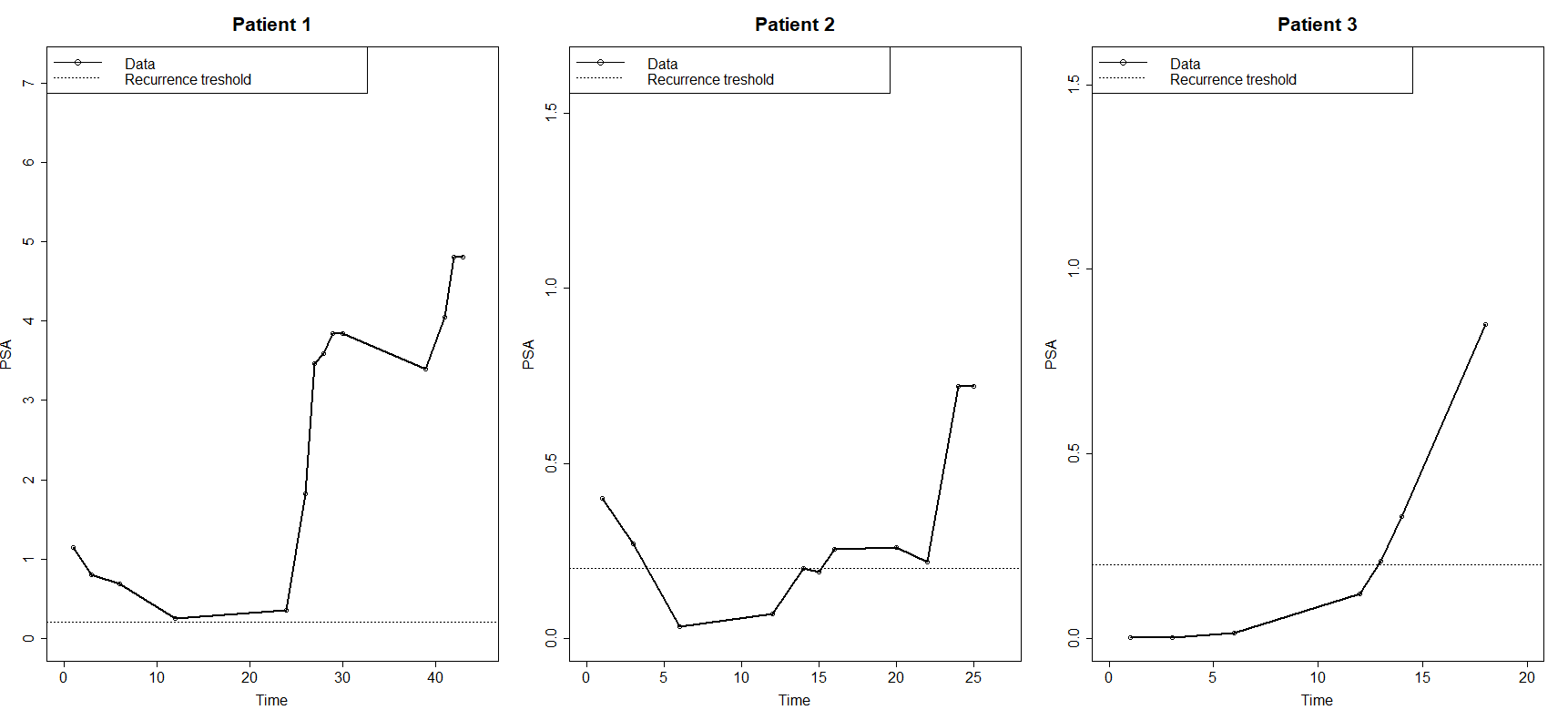
Figure 2: PSA measurements collected on three patients

The database is built on clinical practice in the San Luigi Hospital in Turin. In prostate cancer follow up setting post radical prostatectomy (RP), PSA is the main source of information to base clinical decisions regarding interventions such as PET-PSMA exam. We have $m=111$ patients and, for each of them, we have several demographic and clinical variables, the PSA measurements, and PET-PSMA results, taken at different times after RP. The number of time points in $\mathcal{T}_{y,i}$ ranges from 4 to 17, while the ones in $\mathcal{T}_{z,i}$ from 1 to 4, and the follow-up period is between 4 and 280 months. We can distinguish between patients who, after prostatectomy, show relatively low values of PSA after RP, but may be eventually be subject to BCR at change point, and BCP patients, who present persistent benign/malignant residual tissue after surgery (conventionally signaled by PSA > 0.2) and are usually treated with therapy to inhibit cancer growth - for them, PSA levels may even initially decrease until a new increase occurs at the change point. The presence of a mixed population of BCR and BCP patients and the possible administration of different therapies make the inference task a very difficult exercise. To present the possible data paths, Figure 2 shows data collected for some patients: the shape of the data for patients is quite different (patients 1 and 2 are BCP, while patient 3 is BCR), but also similar shapes can correspond to quite different PSA values (patient 1 and patient 2).
Before surgery, each patient is assigned to a different category according to the status ($S_{i}$), but some more information is collected at surgery time. In particular, pathological stadiation according to TNM classification and the clinical status of prostate margins. Regarding tumor status $P^{T}_{i}$, the clinicians use four different categories: $T1$ (clinically inapparent tumor), $T2$ (tumor confined within prostate), $T3$ (tumor extends through the prostate capsule), $T4$ (tumor is fixed or invades adjacent structures). For the sake of simplicity, here the 4 tumor categories have been reduced to two: $P^{T}_{i}=0$ if $T_{1}$ and $T_{2}$ and $P^{T}_{i}=1$ otherwise. Moreover, the clinical stage of the tumor is usually represented using the Gleason Score [6], and we reduced the original nine categories to two: $S_{i}=0$ if Gleason Score is less than 6 or if it is equal to 3+4, $S_{i}=1$ otherwise.

According to clinical evaluation, each patient with BCR and/or BCP can then be administered four different therapies: adjuvant or salvage androgen deprivation (ormono therapy), adjuvant or salvage radiotherapy. Some patients also underwent regional lymphadenectomy. Adjuvant therapies are administered within 6 months from surgery, while salvage ones are performed after six months on from surgery. In addition, for each patient, we know the age $A_{i}$. All these data are used as clinical and demographic covariates to gain information useful for our model. We estimated three models with different combinations of covariates $\mathbf{C}_{\mu}$, $\mathbf{C}_{\gamma}$, $\mathbf{C}_{\pi}$, all suggested by clinical evidence, and among them, we selected the best model using the WAIC[11] criterion (see Table 3 ). The results we describe refer to the best configuration selected, namely model 2. In Table 5, 6,7, and 8 we show the global parameter estimates for the best model, with relative $95\%$ Credible Intervals. Interpretation of coefficients can be difficult and misleading, particularly when referring to therapies. These are the usual difficulties in interpreting causality with observational and clinical practice databases rather than clinical trials. From a clinical perspective, one could expect therapies to decrease the PSA level before change point $\tau$ and to reduce the growth speed after it. However, the analysis is not targeting therapeutic efficacy. Therapies are used here as indicators of the severity of the disease rather than for estimating their effect. For this reason, we report the logistic analyses used to determine the relationship between administrations of therapies and baseline covariates (see Table 4), where it is easy to notice that, as expected, patients with the worst clinical situation at the surgery time have higher probabilities of receiving one or more of the analyzed therapies. On the other hand, baseline covariates have relatively simple interpretations. Following the theory, PSA decreasing level turns out to be almost zero for patients that do not receive therapies (see $\alpha_{\mu}[1]$). Gleason score is a significant factor, as higher levels determine an increase in PSA values. In particular, the standard deviation of decreasing coefficient $\omega_{\mu}$ and increasing coefficient $\omega_{\gamma}$ are quite different. The high level of the former reflects the heterogeneity of the dataset: PSA levels right after surgery and preceding the changing points are different for BCR and BCP. Finally, the probability of a positive PET-PSMA result at time $t$ strongly depends on the PSA level at $t$ (as was to be expected), on the Gleason score, and on lymph nodes implication. In particular, as the PSA level increases, also the probability increases.

Table 4: Clinical dataset - Coefficients of logistic regression on probability to receive therapies. Bold coefficients refer to pvalues<0.005.

Therapy	Intercept	$P^{R}$	$P^{T}$	$P^{N}$	S	A	PSA at surgery
Ormono adjuvant	-3.22	-0.02	-0.46	1.92	1.20	0.46	1.54
Ormono salvage	-1.57	-0.08	-0.95	-0.51	0.90	0.54	-1.39
Radio adjuvant	-2.94	2.21	-0.57	0.92	0.35	-0.30	-0.25
Radio salvage	-3.14	0.52	1.02	-0.70	1.01	0.23	-0.79
Lymphadenectomy	-0.03	-0.26	0.84	NA	1.12	-0.60	0.25

In Figure 3 we show some examples of the model outputs. In the first row, the fitted curves for the selected patients (top part) are shown, where the grey solid regions are used to show the $95\%$ CI for $\tau_{i}$. In the second row, the approximation on the right-hand side of equation (21) is computed using thresholds 0.5, 0.7, and 0.9: as expected, the higher the threshold, the lower the probability. Filled circles and squares are used to indicate the true and negative outcomes of the test, respectively. The posterior distributions of individual parameters $\lambda_{i},\ \tau_{i},\ \gamma_{i},\ \mu_{i},\ a_{i}$ are reported in Figure 4. The posterior distributions of the parameters $\lambda_{i}$ are quite different from each other and deeply reflect the difference between BCP and BCR patients. In particular, it is easy to see that we obtain quite different fits for patients 1 and 2 of type BCP, in comparison with BCR patients 3.

Table 5: Clinical dataset - Results on global parameters for PSA growth curve before change point. Positive coefficients are associated with a lower level of PSA.

Parameter	2.5%	Mean	97.5%
$\alpha_{\mu}[1]$ - Intercept	-10.37	-7.76	-5.81
$\alpha_{\mu}[2]$ - Ormono adj	-0.20	1.84	3.84
$\alpha_{\mu}[3]$ - Ormono salvage	-5.67	-3.18	-0.49
$\alpha_{\mu}[4]$ - Radio adj	-1.66	0.58	2.85
$\alpha_{\mu}[5]$ - Radio salvage	-0.53	1.46	3.36
$\alpha_{\mu}[6]$ - Lymphadenectomy	-1.30	1.13	4.25

Table 6: Clinical dataset - Results on global parameters for PSA growth curve after the change point. Positive coefficients are associated with a higher level of PSA. Positive coefficients are associated with higher probabilities of positive PET-PSMA examinations.

Parameter	2.5%	Mean	97.5%
$\alpha_{\gamma}[1]$ - intercept	-2.99	-2.58	-2.18
$\alpha_{\gamma}[2]-P^{R}$	-0.14	0.20	0.56
$\alpha_{\gamma}[3]-P^{T}$	-0.29	0.08	0.44
$\alpha_{\gamma}[4]-P^{N}$	-0.78	-0.17	0.47
$\alpha_{\gamma}[5]-P^{S}$	0.32	0.64	1.03
$\alpha_{\gamma}[6]$ - Age	-0.25	-0.04	0.14
$\alpha_{\gamma}[7]$ - Ormono adj	0.18	0.71	1.28
$\alpha_{\gamma}[8]$ - Ormono slv	0.26	0.73	1.28
$\alpha_{\gamma}[9]$ - Radio adj	-1.69	-1.13	0.547
$\alpha_{\gamma}[10]$ - Radio Slv	-0.65	-0.24	0.21
$\alpha_{\gamma}[11]$ - Lymphadenectomy	-0.41	0.03	0.49

Table 7: Clinical dataset - Results on global parameters for logistic model

Parameter	2.5%	Mean	97.5%
$\alpha_{\beta}[1]$ - Intercept	-0.59	0.84	2.34
$\alpha_{\beta}[2]-P^{R}$	-0.11	0.68	1.62
$\alpha_{\beta}[3]-P^{T}$	-0.84	0.22	0.85
$\alpha_{\beta}[4]-P^{N}$	0.05	0.88	2.56
$\alpha_{\beta}[5]-P^{S}$	0.05	1.28	2.56
$\alpha_{\beta}[6]$ - Age	-0.52	-0.14	0.24
$\beta_{1}$	1.64	2.56	3.68
$\beta_{2}$	-0.01	0.00	0.01

Table 8: Clinical dataset - Results on global parameters

Parameter	2.5%	Mean	97.5%
$\omega_{\mu}$	2.53	3.14	3.91
$\omega_{\gamma}$	0.63	0.75	0.90
$\Psi_{a}$	-0.41	-0.26	-0.13
$\omega_{a}$	0.57	0.66	0.76
$a_{\sigma^{2}}$	2.00	2.01	2.02
$b_{\sigma^{2}}$	0.18	0.22	0.27

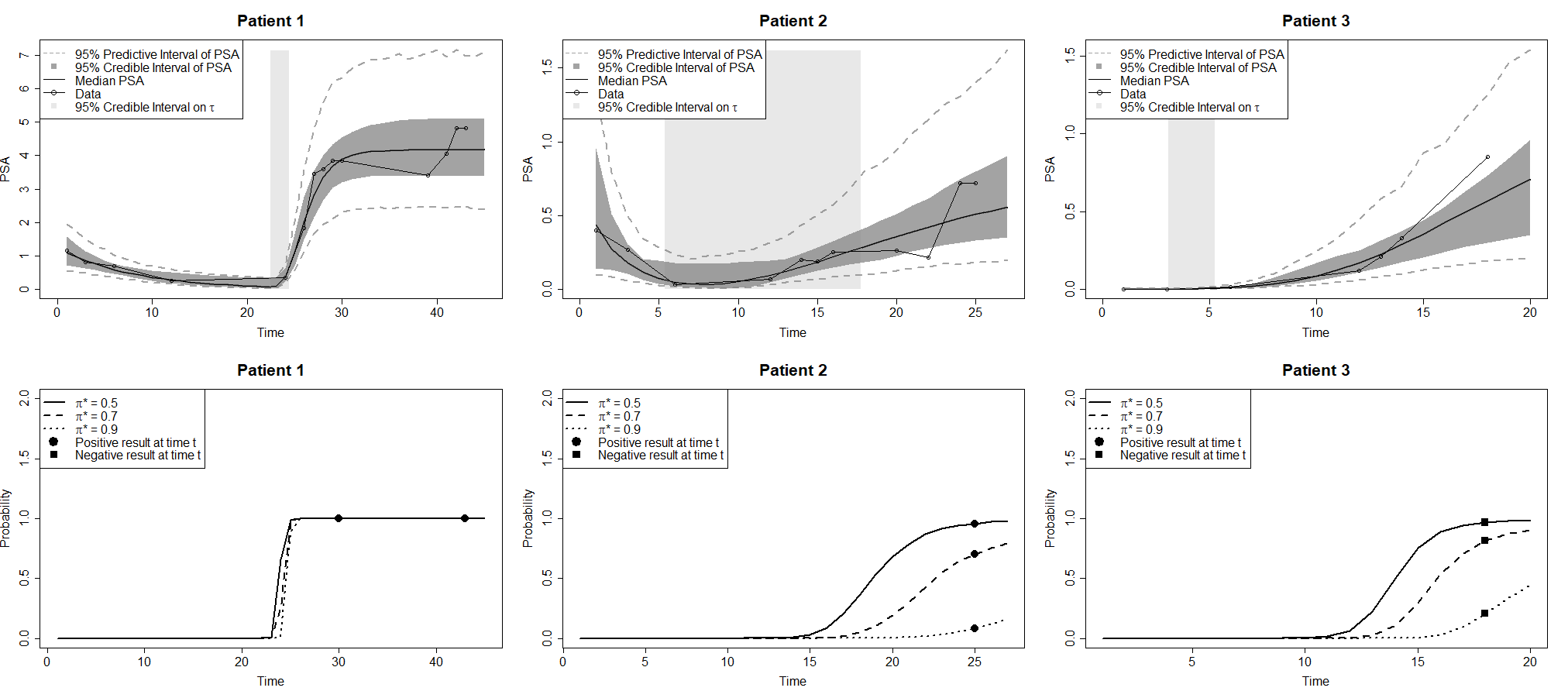
Figure 3: PSA growth curves and probability curves for three patients. Patient 1 and 2 are BCP but with quite different PSA levels, while 3 is BCR.

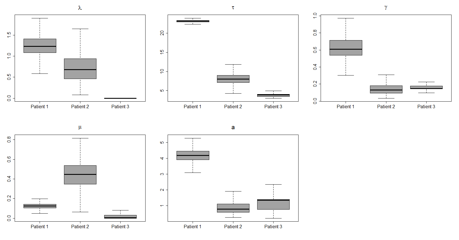
Figure 4: Individual parameters posterior distributions for three patient under analysis.

6 Conclusions

Correct and quick identification of the locations of possible metastasis in prostate cancer is a challenging open problem. Despite the availability of several new techniques and devices, their calibration is still crucial to achieve optimal results. In particular, the results obtained using the sensitive nuclear examination known as PET-PSMA can be really improved if correctly combined with a good estimation of the optimal time to perform the examination. We have proposed a strategy to estimate the optimal time to perform PET-PSMA which exploits information from all the history data of each patient treated. We have introduced the joint-modeling approach, addressing both PSA growth and the probability of a positive PET-PSMA through a logistic model. Finally, we have discussed the optimal time estimation. We have applied the proposed model to both simulated and real data. Simulations were used to test the proposed model under challenging settings. In particular, we showed that the resurgence changing point time $\tau$ is quite a difficult parameter to estimate, as well as the regressive parameters entering the mean of the random effects. On the other hand, simulations also highlight the adaptability of the method to quite different growth patterns of PSA. The results obtained on real data give new insights. Both the growth model estimated patterns and the logistic results are in accordance with clinical evidence.

Data Availability statement

The participants of this study did not give written consent for their data to be shared publicly, so due to the sensitive nature of the research supporting data is not available.

References

- [1] A. Afshar-Oromieh, T. Holland-Letz, F. L. Giesel, C. Kratochwil, W. Mier, S. Haufe, N. Debus, M. Eder, M. Eisenhut, M. Schäfer, et al. Diagnostic performance of 68ga-psma-11 (hbed-cc) pet/ct in patients with recurrent prostate cancer: evaluation in 1007 patients. European journal of nuclear medicine and molecular imaging, 44(8):1258–1268, 2017.
- [2] C. Andrieu and J. Thoms. A tutorial on adaptive mcmc. Statistics and computing, 18(4):343–373, 2008.
- [3] S. Brooks. Markov chain monte carlo method and its application. Journal of the royal statistical society: series D (the Statistician), 47(1):69–100, 1998.
- [4] H. B. Carter, J. D. Pearson, E. J. Metter, L. J. Brant, D. W. Chan, R. Andres, J. L. Fozard, and P. C. Walsh. Longitudinal evaluation of prostate-specific antigen levels in men with and without prostate disease. Jama, 267(16):2215–2220, 1992.
- [5] S. H. Chen and C. A. Pollino. Good practice in bayesian network modelling. Environmental Modelling & Software, 37:134–145, 2012.
- [6] L. Egevad, T. Granfors, L. Karlberg, A. Bergh, and P. Stattin. Prognostic value of the gleason score in prostate cancer. BJU international, 89(6):538–542, 2002.
- [7] Eiber, Matthias and Herrmann, Ken and Fendler, Wolfgang P and Maurer, Tobias. 68 Ga-labeled Prostate-specific Membrane Antigen Positron Emission Tomography for Prostate Cancer Imaging: The New Kid on the Block-Early or Too Early to Draw Conclusions?, 2013. Online; accessed 29 January 2014.
- [8] W. P. Fendler, J. Calais, M. Eiber, R. R. Flavell, A. Mishoe, F. Y. Feng, H. G. Nguyen, R. E. Reiter, M. B. Rettig, S. Okamoto, et al. Assessment of 68ga-psma-11 pet accuracy in localizing recurrent prostate cancer: a prospective single-arm clinical trial. JAMA oncology, 5(6):856–863, 2019.
- [9] N. Fossati, G. Gandaglia, A. Briganti, and F. Montorsi. The emerging role of pet-ct scan after radical prostatectomy: still a long way to go. The Lancet Oncology, 20(9):1193–1195, 2019.
- [10] D. Gamerman and H. F. Lopes. Markov Chain Monte Carlo Stochastic Simulation for Bayesian Inference. CRC Press, second edition, 2006.
- [11] A. Gelman, J. Hwang, and A. Vehtari. Understanding predictive information criteria for bayesian models. Statistics and computing, 24(6):997–1016, 2014.
- [12] Y. Hirata, K. Akakura, C. S. Higano, N. Bruchovsky, and K. Aihara. Quantitative mathematical modeling of psa dynamics of prostate cancer patients treated with intermittent androgen suppression. Journal of molecular cell biology, 4(3):127–132, 2012.
- [13] M. A. Hoffmann, H.-G. Buchholz, H. J. Wieler, T. Höfner, J. Müller-Hübenthal, L. Trampert, and M. Schreckenberger. The positivity rate of 68gallium-psma-11 ligand pet/ct depends on the serum psa-value in patients with biochemical recurrence of prostate cancer. Oncotarget, 10(58):6124, 2019.
- [14] H. B. Luiting, P. J. van Leeuwen, S. Remmers, M. Donswijk, M. B. Busstra, I. L. Bakker, T. Brabander, M. Stokkel, H. G. van der Poel, and M. J. Roobol. Optimal timing of prostate specific membrane antigen positron emission tomography/computerized tomography for biochemical recurrence after radical prostatectomy. The Journal of Urology, 204(3):503–510, 2020.
- [15] J. Pearson, P. Kaminski, E. Metter, J. Fozard, L. Brant, C. Morrell, and H. Carter. Modeling longitudinal rates of change in prostate specific antigen during aging. In Proceedings of the American Statistical Association Meetings: Social Statistics Section, pages 580–585. American Statistical Association, 1991.
- [16] R. Pereira Mestre, G. Treglia, M. Ferrari, M. Pascale, C. Mazzara, N. C. Azinwi, A. Llado’, A. Stathis, L. Giovanella, and E. Roggero. Correlation between psa kinetics and psma-pet in prostate cancer restaging: A meta-analysis. European journal of clinical investigation, 49(3):e13063, 2019.
- [17] N. G. Polson, J. G. Scott, and J. Windle. Bayesian inference for logistic models using pólya–gamma latent variables. Journal of the American statistical Association, 108(504):1339–1349, 2013.
- [18] C. Proust-Lima and J. M. Taylor. Development and validation of a dynamic prognostic tool for prostate cancer recurrence using repeated measures of posttreatment psa: a joint modeling approach. Biostatistics, 10(3):535–549, 2009.
- [19] N. Regula, V. Kostaras, S. Johansson, C. Trampal, E. Lindström, M. Lubberink, I. Velikyan, and J. Sörensen. Comparison of 68ga-psma-11 pet/ct with 11c-acetate pet/ct in re-staging of prostate cancer relapse. Scientific reports, 10(1):1–10, 2020.
- [20] E. H. Slate and K. A. Cronin. Changepoint modeling of longitudinal psa as a biomarker for prostate cancer. In Case studies in Bayesian statistics, pages 435–456. Springer, 1997.
- [21] K. M. Tjørve and E. Tjørve. The use of gompertz models in growth analyses, and new gompertz-model approach: An addition to the unified-richards family. PloS one, 12(6):e0178691, 2017.
- [22] A. A. Tsiatis and M. Davidian. Joint modeling of longitudinal and time-to-event data: an overview. Statistica Sinica, pages 809–834, 2004.
- [23] F. A. Verburg, D. Pfister, A. Heidenreich, A. Vogg, N. I. Drude, S. Vöö, F. M. Mottaghy, and F. F. Behrendt. Extent of disease in recurrent prostate cancer determined by [68ga] psma-hbed-cc pet/ct in relation to psa levels, psa doubling time and gleason score. European journal of nuclear medicine and molecular imaging, 43(3):397–403, 2016.