Real roots of real cubics and optimization

Abstract

The solution of the cubic equation has a century-long history; however, the usual presentation is geared towards applications in algebra and is somewhat inconvenient to use in optimization where frequently the main interest lies in real roots.

In this note, we present the roots of the cubic in a form that makes them convenient to use and we also focus on information on the location of the real roots. Armed with this, we provide several applications in optimization where we compute Fenchel conjugates, proximal mappings and projections.

2020 Mathematics Subject Classification: Primary 90C25; Secondary 12D10, 26C10, 90C26

Keywords: Convex quartic, cubic equation, cubic polynomial, Fenchel conjugate, projection, proximal mapping, root.

1 Introduction

The history of solving cubic equations is rich and centuries old; see, e.g., Confalonieri’s recent book [7] on Cardano’s work. Cubics do also appear in convex and nonconvex optimization. However, treatises on solving the cubic often focus on the general complex case making the results less useful to optimizers. The purpose of this note is two-fold. We present a largely self-contained derivation of the solution of the cubic with an emphasis on usefulness to practitioners. We do not claim novelty of these results; however, the presentation appears to be particularly convenient. We then turn to novel results. We show how the formulas can be used to compute Fenchel conjugates and proximal mappings of some convex functions. We also discuss projections on convex and nonconvex sets.

1.1 Outline of the paper

The paper is organized as follows. In Section 1.2, we collect some facts on polynomials. Section 2 contains a self-contained treatment of the depressed cubic; in turn, this leads quickly to counterparts for the general cubic in Section 3. Section 4 concerns convex quartics — we compute their Fenchel conjugates and proximal mappings. In Section 5, we present a formula for the proximal mapping of the convex reciprocal function. An explicit formula for the projection onto the epigraph of a parabola is provided in Section 6. In Section 7, we derive a formula for the projection of certain points onto a rectangular hyperbolic paraboloid. In the final Section 8, we revisit the proximal mapping of the closure of a perspective function.

1.2 Some facts

We now collect some properties of polynomials that are well known; as a reference, we recommend [10].

Fact 1.1.

Let $f(x)$ be a nonconstant complex polynomial and let $r\in\mathbb{C}$ such that $f(r)=0$. Then the multiplicity of $r$ is is the smallest integer $k$ such that the $k$th derivative at $r$ is nonzero: $f^{(k-1)}(r)=0$ and $f^{(k)}(r)\neq 0$. When $k=1$, $2$, or $3$, then we say that $r$ is a simple, double, or triple root, respectively.

Fact 1.2.

(Vieta) Suppose $f(x)=ax^{3}+bx^{2}+cx+d$ is a cubic polynomial (i.e., $a\neq 0$) with complex coefficients. If $r_{1},r_{2},r_{3}$ denote the (possibly repeated and complex) roots of $f$, then

$$r_{1}+r_{2}+r_{3} =-\frac{b}{a}$$ (1a)

$$r_{1}r_{2}+r_{1}r_{3}+r_{2}r_{3} =\frac{c}{a}$$ (1b)

$$r_{1}r_{2}r_{3} =-\frac{d}{a}.$$ (1c)

Conversely, if $r_{1},r_{2},r_{3}$ in $\mathbb{C}$ satisfy 1, then they are the (possibly repeated) roots of $f$.

Fact 1.3.

Suppose $f(x)=ax^{3}+bx^{2}+cx+d$ is a cubic polynomial (i.e., $a\neq 0$) with real coefficients. Then $f$ has three (possibly complex) roots (counting multiplicity). More precisely, exactly one of the following holds:

1. $f$ has exactly one real root which either is simple (and the two remaining roots are nonreal simple roots and conjugate to each other) or is a triple root.

2. $f$ has exactly two distinct real roots: one is simple and the other double.

3. $f$ has exactly three distinct simple real roots.

Remark 1.4.

We mention that the roots of a polynomial of a fixed degree depend continuously on the coefficients — see [10, Theorem 1.3.1] for a precise statement and also the other results in [10, Section 1.3].

2 The depressed cubic

In this section, we study the depressed cubic

$$g(z):=z^{3}+pz+q,\quad\text{where}\;\;p\in\mathbb{R}\;\;\text{and}\;\;q\in\mathbb{R}.$$ (2)

Theorem 2.1.

We have

$$g^{\prime}(z)=3z^{2}+p\;\;\text{and}\;\;g^{\prime\prime}(z)=6z.$$ (3)

Then $0$ is the only inflection point of $g$: $g$ is strictly concave on $\mathbb{R}_{-}$ and $g$ is strictly convex on $\mathbb{R}_{+}$.

Moreover, exactly one of the following cases occurs:

1. $p<0$: Set $z_{\pm}:=\pm\sqrt{-p/3}$. Then $z_{-}<z_{+}$, $z_{\pm}$ are two distinct simple roots of $g^{\prime}$, $g$ is strictly increasing on $\left]-\infty,z_{-}\right]$, $g$ is strictly decreasing on $[z_{-},z_{+}]$, $g$ is strictly increasing on $\left[z_{+},+\infty\right[$. Moreover,

   $$g(z_{-})g(z_{+})=4\Delta,\quad\text{where}\;\;\Delta:=(p/3)^{3}+(q/2)^{2},$$ (4)

   and this case trifurcates further as follows:

   1. $\Delta>0$: Then $g$ has exactly one real root $r$. It is simple and given by

      $$r:=u_{-}+u_{+},\quad\text{where}\;\;u_{\pm}:=\sqrt[3]{\frac{-q}{2}\pm\sqrt{\Delta}}.$$ (5)

      The two remaining simple nonreal roots are

      $$-\tfrac{1}{2}(u_{-}+u_{+})\pm\mathrm{i}\tfrac{1}{2}\sqrt{3}(u_{-}-u_{+}).$$ (6)

   2. $\Delta=0$: If $q>0$ (resp. $q<0$), then $2z_{-}$ (resp. $2z_{+}$) is a simple real root while $z_{+}$ (resp. $z_{-}$) is a double root. Moreover, these cases can be combined into

      $$\frac{3q}{p}=2\sqrt[3]{\frac{-q}{2}}\;\text{is a simple root of $g$}\;\;\text{and}\;\;\frac{-3q}{2p}=-\sqrt[3]{\frac{-q}{2}}\;\text{is a double root of $g$.}$$ (7)

   3. $\Delta<0$: Then $g$ has three simple real roots $r_{-},r_{0},r_{+}$ where $r_{-}<z_{-}<r_{0}<z_{+}<r_{+}$. Indeed, set

      $$\theta:=\arccos\frac{-q/2}{(-p/3)^{3/2}},$$ (8)

      which lies in $\left]0,\pi\right[$, and then define $z_{0},z_{1},z_{2}$ by

      $$z_{k}:=2(-p/3)^{1/2}\cos\Big{(}\frac{\theta+2k\pi}{3}\Big{)}.$$ (9)

      Then $r_{-}=z_{1}$, $r_{0}=z_{2}$, and $r_{+}=z_{0}$.

2. $p=0$: Then $g^{\prime}$ has a double root at $0$, and $g$ is strictly increasing on $\mathbb{R}$. The only real root is

   $$r:=(-q)^{1/3}.$$ (10)

   If $q=0$, then $r$ is a triple root. If $q\neq 0$, then $r$ is a simple root and the remaining nonreal simple roots are $-\tfrac{1}{2}r\pm\mathrm{i}\tfrac{1}{2}\sqrt{3}r$.

3. $p>0$: Then $g^{\prime}$ has no real root, $g$ is strictly increasing on $\mathbb{R}$, and $g$ has exactly one real root $r$. It is simple and given by

   $$r:=u_{-}+u_{+},\quad\text{where}\;\;u_{\pm}:=\sqrt[3]{\frac{-q}{2}\pm\sqrt{\Delta}}\;\;\text{and}\;\;\Delta:=(p/3)^{3}+(q/2)^{2}.$$ (11)

   Once again, the two remaining simple nonreal roots are

   $$-\tfrac{1}{2}(u_{-}+u_{+})\pm\mathrm{i}\tfrac{1}{2}\sqrt{3}(u_{-}-u_{+}).$$ (12)

Proof. Except for the formulas for the roots, all statements on $g$ follow from standard calculus.

(i)(a): Because $\Delta>0$ and $g$ is strictly decreasing on $[z_{-},z_{+}]$, it follows from 4 that $g$ has the same sign on $[z_{-},z_{+}]$ and so $g$ has no root in that interval. Now $g$ is strictly increasing on $\left]-\infty,z_{-}\right]$ and on $\left[z_{+},+\infty\right[$; hence, $g$ has exactly one real root $r$ and it lies outside $[z_{-},z_{+}]$. Note that $r$ must be simple because the roots of $g^{\prime}$ are $z_{\mp}$ and $r\neq z_{\mp}$. Note that $u_{-}<u_{+}$. Next, $u_{-}^{3}u_{+}^{3}=(q/2)^{2}-\Delta=-(p/3)^{3}$ and so

$$u_{-}u_{+}=-p/3.$$ (13)

Also,

$$u_{-}^{3}+u_{+}^{3}=\frac{-q}{2}-\sqrt{\Delta}+\frac{-q}{2}+\sqrt{\Delta}=-q.$$ (14)

Hence

$$g(r) =r^{3}+pr+q$$

$$=(u_{-}+u_{+})^{3}+p(u_{-}+u_{+})+q$$

$$=u_{-}^{3}+u_{+}^{3}+3u_{-}u_{+}(u_{-}+u_{+})+p(u_{-}+u_{+})+q$$

$$=\big{(}u_{-}^{3}+u_{+}^{3}\big{)}+(3u_{-}u_{+}+p)(u_{-}+u_{+})+q$$

$$=-q+\big{(}3(-p/3)+p\big{)}(u_{-}+u_{+})+q$$ (using 13 and 14)

$$=0$$

as claimed. Observe that we only need the properties 13 and 14 about $u_{-},u_{+}$ to conclude that $u_{-}+u_{+}$ is a root of $g$. This observation leads us quickly to the two remaining complex roots: First, denote the primitive 3rd root of unity by $\omega$, i.e.,

$$\omega:=\exp(2\pi\mathrm{i}/3)=\cos(2\pi/3)+\mathrm{i}\sin(2\pi/3)=-\tfrac{1}{2}+\mathrm{i}\tfrac{1}{2}\sqrt{3}.$$ (15)

Then $\omega^{2}=\overline{\omega}=-\tfrac{1}{2}-\mathrm{i}\tfrac{1}{2}\sqrt{3}$ and $\omega^{3}=\overline{\omega}^{3}=1$. Now set

$$v_{-}:=\omega u_{-}\;\;\text{and}\;\;v_{+}:=\omega^{2}u_{+}=\overline{\omega}u_{+}.$$

Then $v_{-}v_{+}(\omega u_{-})=(\omega^{2}u_{+})=\omega^{3}u_{-}u_{+}=u_{-}u_{+}=-p/3$ by 13, and $v_{-}^{3}+v_{+}^{3}=(\omega u_{-})^{3}+(\omega^{2}u_{+})^{3}=\omega^{3}u_{-}^{3}+\omega^{6}u_{+}^{3}=u_{-}^{3}+u_{+}^{3}=-q$ by 13. Hence

$$v_{-}+v_{+} =\omega u_{-}+\overline{\omega}u_{+}$$

$$=\big{(}-\tfrac{1}{2}+\mathrm{i}\tfrac{1}{2}\sqrt{3}\big{)}u_{-}+\big{(}-\tfrac{1}{2}-\mathrm{i}\tfrac{1}{2}\sqrt{3}\big{)}u_{+}$$

$$=-\tfrac{1}{2}(u_{-}+u_{+})+\mathrm{i}\tfrac{1}{2}\sqrt{3}(u_{-}-u_{+})$$

and its conjugate are the remaining simple complex roots of $g$.

(i)(b): From 4, it follows that $z_{-}$ or $z_{+}$ is a root of $g$. In view of 1.1 and $g^{\prime}(z_{-})=g^{\prime}(z_{+})$, it follows that one of $z_{-},z_{+}$ is at least a double root, but not both; moreover, it cannot be a triple root because $0$ is the only root of $g^{\prime\prime}$ and $z_{-}<0<z_{+}$. Hence exactly one of $z_{-},z_{+}$ is a double root. To verify the remaining parts, we first define

$$r_{1}:=\frac{3q}{p}\;\;\text{and}\;\;r_{2}:=\frac{-3q}{2p}.$$

Because $\Delta=0$, it follows that $4p^{3}+27q^{2}=0$. Hence

$$g(r_{1}) =r_{1}^{3}+pr_{1}+q=\frac{27q^{3}}{p^{3}}+\frac{3pq}{p}+q=\frac{27q^{3}}{p^{3}}+4q=\frac{q}{p^{3}}\big{(}27q^{2}+4p^{3}\big{)}=0$$

and

$$g(r_{2}) =r_{2}^{3}+pr_{2}+q=\frac{-27q^{3}}{8p^{3}}+\frac{-3pq}{2p}+q=\frac{-27q^{3}}{8p^{3}}-\frac{q}{2}=\frac{-q}{8p^{3}}\big{(}27q^{2}+4p^{3}\big{)}=0.$$

The assumption that $\Delta=0$ readily yields

$$p=\frac{-3^{1/3}q^{2/3}}{2^{2/3}}\;\;\text{and}\;\;|q|=\frac{2(-p)^{3/2}}{3^{3/2}}.$$

Hence

$$r_{1}=3qp^{-1}=3q(-1)3^{-1/3}q^{-2/3}2^{2/3}=2^{2/3}(-q)^{1/3}$$

and

$$r_{2}=-3q2^{-1}p^{-1}=-3q2^{-1}(-1)3^{-1/3}q^{-2/3}2^{2/3}=-2^{-1/3}(-q)^{1/3}$$

as claimed.

If $q>0$, then

$$r_{1}=\frac{3q}{p}=\frac{3\cdot 2(-p)^{3/2}}{3^{3/2}p}=-2(-p/3)^{1/2}=2z_{-}$$

and

$$r_{2}=\frac{-3q}{2p}=-\tfrac{1}{2}\frac{3q}{p}=-\tfrac{1}{2}r_{1}=-\tfrac{1}{2}2z_{-}=z_{+}.$$

Similarly, if $q<0$, then $r_{1}=2z_{+}$ and $r_{2}=z_{-}$.

No matter the sign of $q$, we have $r_{2}\in\{z_{-},z_{+}\}$ and thus $g^{\prime}(r_{2})=0$, i.e., $r_{2}$ is the double root.

(i)(c): In view of 4, $g(z_{-})$ and $g(z_{+})$ have opposite signs. Because $g$ is strictly decreasing on $[z_{-},z_{+}]$, it follows that $g(z_{-})>0>g(z_{+})$. Hence there is at least on real root $r_{0}$ in $\left]z_{-},z_{+}\right[$. On the other hand, $g$ is strictly increasing on $\left]-\infty,z_{-}\right]$ and on $\left[z_{+},+\infty\right[$ which yields further roots $r_{-}$ and $r_{+}$ as announced. Having now three real roots, they must all be simple.

Next, note that $\Delta<0$ $\Leftrightarrow$ $0\leq(q/2)^{2}<-(p/3)^{3}=(-p/3)^{3}$ $\Leftrightarrow$ $0\leq(q/2)^{2}/(-p/3)^{3}<1$ $\Leftrightarrow$ $0\leq(|q|/2)/(-p/3)^{3/2}<1$ $\Leftrightarrow$ $-1<(-q/2)/(-p/3)^{3/2}<1$. It follows that

$$\theta=\arccos\frac{-q/2}{(-p/3)^{3/2}}\in\left]0,\pi\right[$$ (16)

as claimed. For convenience, we set, for $k\in\{0,1,2\}$,

$$\theta_{k}:=\frac{\theta+2k\pi}{3};\quad\text{hence,}\;\;z_{k}=2(-p/3)^{1/2}\cos(\theta_{k}).$$ (17)

Recall that $0<\theta<\pi$, which allows us to draw three conclusions:

$$0<\theta_{0}=\theta/3<\pi/3 \Rightarrow 1>\cos(\theta_{0})=\cos(\theta/3)>1/2;$$ (18a)

$$2\pi/3<\theta_{1}=(\theta+2\pi)/3<\pi \Rightarrow-1/2>\cos(\theta_{1})=\cos((\theta+2\pi)/3)>-1;$$ (18b)

$$4\pi/3<\theta_{2}=(\theta+4\pi)/3<5\pi/3 \Rightarrow-1/2<\cos(\theta_{2})=\cos((\theta+2\pi)/3)<1/2.$$ (18c)

Hence $\cos(\theta_{1})<\cos(\theta_{2})<\cos(\theta_{0})$ and thus

$$z_{1}<z_{2}<z_{0}.$$ (19)

All we need to do is to verify that each $z_{k}$ is actually a root of $g$. To this end, observe first that the triple-angle formula for the cosine (see, e.g., [2, Formula 4.3.28 on page 72]) yields

$$\cos^{3}(\theta_{k}) =\frac{3\cos(\theta_{k})+\cos(3\theta_{k})}{4}=\frac{3\cos(\theta_{k})+\cos(\theta+2k\pi)}{4}$$ (20a)

$$=\frac{3\cos(\theta_{k})+\cos(\theta)}{4}.$$ (20b)

Then

$$g(z_{k}) =z_{k}^{3}+pz_{k}+q$$

$$=8(-p/3)^{3/2}\cos^{3}(\theta_{k})+p2(-p/3)^{1/2}\cos(\theta_{k})+q$$

$$=2(-p/3)^{3/2}\big{(}3\cos(\theta_{k})+\cos(\theta)\big{)}+2(-p/3)^{1/2}p\cos(\theta_{k})+q$$ (using 20)

$$=2(-p/3)^{1/2}\cos(\theta_{k})\big{(}3(-p/3)+p\big{)}+2(-p/3)^{3/2}\cos(\theta)+q$$

$$=2(-p/3)^{3/2}\cos(\theta)+q$$

$$=2(-p/3)^{3/2}\frac{-q/2}{(-p/3)^{3/2}}+q$$ (using 16)

$$=0,$$

and this completes the proof for this case.

(ii): If $q=0$, then $g(z)=z^{3}$ so $z=0$ is the only root of $g$ and it is of multiplicity $3$. Thus we assume that $q\neq 0$. Then $g(z)=0$ $\Leftrightarrow$ $z^{3}+q=0$ $\Leftrightarrow$ $z^{3}=-q$ $\Rightarrow$ $z=(-q)^{1/3}\neq 0$. Because $g$ is strictly increasing on $\mathbb{R}$, $r:=(-q)^{1/3}$ is the only real root of $g$. Because $g^{\prime}$ has only one real root, namely $0$, it follows that $g^{\prime}(r)\neq 0$ and so $r$ is a simple root. Denoting again by $\omega$ the primitive 3rd root of unity (see 15), it is clear that the remaining complex (simple) roots are $\omega r$ and $\overline{\omega}r$ as claimed.

(iii): Note that $\Delta\geq(p/3)^{3}>0$ because $p>0$. The fact that $r$ is a root is shown exactly as in (i)(a). It is simple because $g^{\prime}$ has no real roots, and $r$ is unique because $g$ is strictly increasing. The complex roots are derived exactly as in (i)(a). $\hfill\quad\blacksquare$

We now provide a conise version of Theorem 2.1:

Corollary 2.2.

(trichotomy) Set $\Delta:=(p/3)^{3}+(q/2)^{2}$. Then exactly one of the following holds:

1. $p=0$ or $\Delta>0$: Then $g$ has exactly one real root and it is given by

   $$\sqrt[3]{\frac{-q}{2}+\sqrt{\Delta}}+\sqrt[3]{\frac{-q}{2}-\sqrt{\Delta}}.$$ (21)

2. $p<0$ and $\Delta=0$: Then $g$ has exactly two real roots which are given by

   $$\frac{3q}{p}=2\sqrt[3]{\frac{-q}{2}}\;\;\text{and}\;\;\frac{-3q}{2p}=-\sqrt[3]{\frac{-q}{2}}.$$ (22)

3. $\Delta<0$: Then $g$ has exactly three real roots $z_{0},z_{1},z_{2}$ which are given by

   $$z_{k}:=2(-p/3)^{1/2}\cos\Big{(}\frac{\theta+2k\pi}{3}\Big{)},\quad\text{where}\;\;\theta:=\arccos\frac{-q/2}{(-p/3)^{3/2}},$$ (23)

   and where $z_{1}<z_{2}<z_{0}$.

3 The general cubic

In this section, we turn to the general cubic

$$f(x):=ax^{3}+bx^{2}+cx+d,\quad\text{where}\;\;a,b,c,d\;\text{are in}\;\mathbb{R}\;\text{and}\;a>0.$$ (24)

(The case $a<0$ is treated similarly.) Note that $f^{\prime\prime}(x)=6ax+2b$ has exactly one zero, namely

$$x_{0}:=\frac{-b}{3a}.$$ (25)

The change of variables

$$x=z+x_{0}$$ (26)

leads to the well known depressed cubic

$$g(z):=z^{3}+pz+q,\;\;\text{where}\;\;p:=\frac{3ac-b^{2}}{3a^{2}}\;\;\text{and}\;\;q:=\frac{27a^{2}d+2b^{3}-9abc}{27a^{3}}$$ (27)

which we reviewed in Section 2. Here $ag(z)=f(x)=f(z+x_{0})$ so the roots of $g$ are precisely those of $f$, translated by $x_{0}$:

$$x f \Leftrightarrow x-x_{0} g$$ is a root of is a root of . (28)

So all we need to do is find the roots of $g$, and then add $x_{0}$ to them, to obtain the roots of $f$. Because the change of variables 26 is linear, multiplicity of the roots are preserved. Translating some of the results from Theorem 2.1 for $g$ to $f$ gives the following:

Theorem 3.1.

$f$ is strictly concave on $\left]-\infty,x_{0}\right]$ and is strictly convex on $\left[x_{0},+\infty\right[$, where $x_{0}$ is the unique inflection point of $f$ defined in 25. Recall the definitions of $p,q$ from 27 and also set

$$\Delta:=(p/3)^{3}+(q/2)^{2}=\frac{(3ac-b^{2})^{3}}{(9a^{2})^{3}}+\frac{(27a^{2}d+2b^{3}-9abc)^{2}}{(54a^{3})^{2}}.$$ (29)

Then exactly one of the following cases occurs:

1. $b^{2}>3ac\Leftrightarrow p<0$ : Set $x_{\pm}:=(-b\pm\sqrt{b^{2}-3ac})/(3a)$. Then $x_{\pm}$ are two distinct simple roots of $f^{\prime}$, $f$ is strictly increasing on $\left]-\infty,x_{-}\right]$, $f$ is strictly decreasing on $[x_{-},x_{+}]$, $f$ is strictly increasing on $\left[x_{+},+\infty\right[$. This case trifurcates further as follows:

   1. $\Delta>0$ : Then $f$ has exactly one real root; moreover, it is simple and given by

      $$x_{0}+u_{-}+u_{+},\quad\text{where}\;\;u_{\pm}:=\sqrt[3]{\frac{-q}{2}\pm\sqrt{\Delta}}.$$ (30)

      The two remaining simple nonreal roots are $x_{0}-\tfrac{1}{2}(u_{-}+u_{+})\pm\mathrm{i}\tfrac{1}{2}\sqrt{3}(u_{-}-u_{+})$.

   2. $\Delta=0$ : Then $f$ has two distinct real roots: The simple root is

      $$x_{0}+\frac{3q}{p}=x_{0}+2\sqrt[3]{\frac{-q}{2}}=\frac{4abc-b^{3}-9a^{2}d}{a{\left(b^{2}-3ac\right)}}$$ (31)

      and the double root is

      $$x_{0}-\frac{3q}{2p}=x_{0}-\sqrt[3]{\frac{-q}{2}}=\frac{9ad-bc}{2(b^{2}-3ac)}.$$ (32)

   3. $\Delta<0$ : Then $f$ has three simple real roots $r_{-},r_{0},r_{+}$ where $r_{-}<x_{-}<r_{0}<x_{+}<r_{+}$. Indeed, set

      $$\theta:=\arccos\frac{-q/2}{(-p/3)^{3/2}},$$ (33)

      which lies in $\left]0,\pi\right[$, and then define $y_{0},y_{1},y_{2}$ by

      $$y_{k}:=x_{0}+2(-p/3)^{1/2}\cos\Big{(}\frac{\theta+2k\pi}{3}\Big{)}.$$ (34)

      Then $r_{-}=y_{1}$, $r_{0}=y_{2}$, and $r_{+}=y_{0}$.

2. $b^{2}=3ac\Leftrightarrow p=0$ : Then $f$ is strictly increasing on $\mathbb{R}$ and its only real root is

   $$r:=x_{0}+(-q)^{1/3}.$$ (35)

   If $q=0$, then $r$ is a triple root. If $q\neq 0$, then $r$ is a simple root and the remaining nonreal simple roots are $x_{0}-\tfrac{1}{2}(-q)^{1/3}\pm\mathrm{i}\tfrac{1}{2}\sqrt{3}(-q)^{1/3}$.

3. $b^{2}<3ac\Leftrightarrow p>0$ : Then $f$ is strictly increasing on $\mathbb{R}$, and $f$ has exactly one real root; moreover, it is simple and given by

   $$x_{0}+u_{-}+u_{+},\quad\text{where}\;\;u_{\pm}:=\sqrt[3]{\frac{-q}{2}\pm\sqrt{\Delta}}.$$ (36)

   The two remaining simple nonreal roots are $x_{0}-\tfrac{1}{2}(u_{-}+u_{+})\pm\mathrm{i}\tfrac{1}{2}\sqrt{3}(u_{-}-u_{+})$.

In turn, Corollary 2.2 turns into

Corollary 3.2.

Recall 25 and 27, and set

$$\Delta:=(p/3)^{3}+(q/2)^{2}=\frac{(3ac-b^{2})^{3}}{(9a^{2})^{3}}+\frac{(27a^{2}d+2b^{3}-9abc)^{2}}{(54a^{3})^{2}}$$ (37)

Then exactly one of the following holds:

1. $b^{2}=3ac$ or $\Delta>0$ : Then $f$ has exactly one real root and it is given by

   $$x_{0}+\sqrt[3]{\frac{-q}{2}+\sqrt{\Delta}}+\sqrt[3]{\frac{-q}{2}-\sqrt{\Delta}}.$$ (38)

2. $b^{2}>3ac$ and $\Delta=0$ : Then $f$ has exactly two real roots which are given by

   $$x_{0}+\frac{3q}{p}=x_{0}+2\sqrt[3]{\frac{-q}{2}}\;\;\text{and}\;\;x_{0}+\frac{-3q}{2p}=x_{0}-\sqrt[3]{\frac{-q}{2}}.$$ (39)

3. $\Delta<0$ : Then $f$ has exactly three real (simple) roots $r_{0},r_{1},r_{2}$, where

   $$r_{k}:=x_{0}+2(-p/3)^{1/2}\cos\Big{(}\frac{\theta+2k\pi}{3}\Big{)},\quad\text{}\;\;\theta:=\arccos\frac{-q/2}{(-p/3)^{3/2}},$$ (40)

   and $r_{1}<r_{2}<r_{0}$.

4 Convex Analysis of the general quartic

In this section, we study the function

$$h(x):=\alpha x^{4}+\beta x^{3}+\gamma x^{2}+\delta x+\varepsilon,\quad\text{where $\alpha,\beta,\gamma,\delta,\varepsilon$ are in $\mathbb{R}$ with $\alpha\neq 0$.}$$ (41)

We start by characterizing convexity.

Proposition 4.1.

(convexity) The general quartic 41 is convex if and only if

$$\alpha>0\;\;\text{and}\;\;8\alpha\gamma\geq 3\beta^{2}.$$ (42)

Proof. Note that $h^{\prime}(x)=4\alpha x^{3}+3\beta x^{2}+2\gamma x+\delta$ and, also completing the square,

$$h^{\prime\prime}(x) =12\alpha x^{2}+6\beta x+2\gamma=\frac{3}{4}\alpha\Big{(}4x+\frac{\beta}{\alpha}\Big{)}^{2}+2\gamma-\frac{3\beta^{2}}{4\alpha}.$$ (43)

Hence $h^{\prime\prime}\geq 0$ $\Leftrightarrow$ [$\alpha>0$ and $2\gamma\geq 3\beta^{2}/(4\alpha)$] $\Leftrightarrow$ 42. (For further information on deciding nonnegativity of polynomials, see [6, Section 3.1.3].) $\hfill\quad\blacksquare$

Having characterization convexity, we shall assume this condition for the remainder of this section:

$$\text{$h$ is convex, i.e.,\;\;}\alpha>0\;\text{and}\;8\alpha\gamma\geq 3\beta^{2}.$$ (44)

Proposition 4.2.

(Fenchel conjugate) Recall our assumptions 41 and 44. Let $y\in\mathbb{R}$. Then

$$h^{*}(y)=yx_{y}-h(x_{y}),$$ (45)

where $p:=(8\alpha\gamma-3\beta^{2})/(16\alpha^{2})\geq 0$, $q:=(8\alpha^{2}(\delta-y)+\beta^{3}-4\alpha\beta\gamma)/(32\alpha^{3})$, $\Delta:=(p/3)^{2}+(q/2)^{2}\geq 0$, and

$$x_{y}:=-\frac{\beta}{4\alpha}+\sqrt[3]{\frac{-q}{2}+\sqrt{\Delta}}+\sqrt[3]{\frac{-q}{2}-\sqrt{\Delta}}.$$ (46)

Proof. Because $h$ is supercoercive, it follows from [3, Proposition 14.15] that $\operatorname{dom}h^{*}=\mathbb{R}$. Combining with the differentiability of $h$, it follows that $y\in\operatorname{int}\operatorname{dom}\,h^{*}\subseteq\operatorname{dom}\partial h^{*}={\operatorname{ran}}\,\partial h={\operatorname{ran}}\,h^{\prime}$. However, if $h^{\prime}(x)=y$, then $h^{*}(y)=xy-h(x)$ and we have found the conjugate. It remains to solve $h^{\prime}(x)=y$, i.e.,

$$4\alpha x^{3}+3\beta x^{2}+2\gamma x+\delta-y=0.$$ (47)

So we set

$$f(x):=ax^{3}+bx^{2}+cx+d,\quad\text{where}\;\;a:=4\alpha,\;\;b:=3\beta,\;\;c:=2\gamma,\;\;d:=\delta-y.$$

To solve 47, i.e., $f(x)=0$, we first note that

$$p =\frac{3ac-b^{2}}{3a^{2}}=\frac{3(4\alpha)(2\gamma)-(3\beta)^{2}}{3(4\alpha)^{2}}=\frac{8\alpha\gamma-3\beta^{2}}{16\alpha^{2}}\geq 0,$$

where the inequality follows from 44. Next,

$$q =\frac{3^{3}a^{2}d+2b^{3}-3^{2}abc}{(3a)^{3}}=\frac{3^{3}4^{2}\alpha^{2}(\delta-y)+2(3^{3}\beta^{3})-3^{2}(4\alpha)(3\beta)(2\gamma)}{3^{3}4^{3}\alpha^{3}}$$

$$=\frac{8\alpha^{2}(\delta-y)+\beta^{3}-4\alpha\beta\gamma}{32\alpha^{3}}$$

and

$$\Delta=(p/3)^{3}+(q/2)^{2}\geq 0,$$

where the inequality follows because $p\geq 0$. Then $-b/(3a)=-\beta/(4\alpha)$ and now Corollary 3.2(i) yields the unique solution of $f(x)=0$ as 46. $\hfill\quad\blacksquare$

Proposition 4.3.

(proximal mapping) Recall our assumptions 41 and 44. Let $y\in\mathbb{R}$. Then

$$\operatorname{Prox}_{h}(y)=-\frac{\beta}{4\alpha}+\sqrt[3]{\frac{-q}{2}+\sqrt{\Delta}}+\sqrt[3]{\frac{-q}{2}-\sqrt{\Delta}},$$ (48)

where

$$p:=\frac{4\alpha(1+2\gamma)-3\beta^{2}}{16\alpha^{2}},\quad q:=\frac{8\alpha^{2}(\delta-y)+\beta^{3}-2\alpha\beta(1+2\gamma)}{32\alpha^{3}},$$ (49)

and $\Delta:=(p/3)^{3}+(q/2)^{2}\geq 0$.

Proof. Because $h$ is differentiable and full domain, it follows that $\operatorname{Prox}_{h}(y)$ is the unique solution $x$ of the equation $h^{\prime}(x)+x-y=0$. The proof thus proceeds analogously to that of Proposition 4.2 — the only difference is we must solve

$$f(x):=ax^{3}+bx^{2}+cx+d,\quad\text{where}\;\;a:=4\alpha,\;\;b:=3\beta,\;\;c:=2\gamma+1,\;\;d:=\delta-y.$$

(The only difference is that $c=2\gamma+1$ rather than $2\gamma$ due to the additional term “$+x$”.) Thus we know a priori that the resulting cubic must have a unique real solution. We now have

$$0 <\frac{1}{4\alpha}\leq\frac{1}{4\alpha}+\frac{8\alpha\gamma-3\beta^{2}}{16\alpha^{2}}=\frac{4\alpha(1+2\gamma)-3\beta^{2}}{16\alpha^{2}}=p=\frac{12\alpha(1+2\gamma)-9\beta^{2}}{48\alpha^{2}}$$

$$=\frac{3ac-b^{2}}{3a^{2}},$$

which is our usual $p$ from discussing roots of the cubic $f$. Similarly, the $q$ defined here is the same as the usual $q$ for $f(x)$ (see 27). Finally, the formula for $x=\operatorname{Prox}_{h}(y)$ now follows from Corollary 3.2(i). $\hfill\quad\blacksquare$

Example 4.4.

Suppose that

$$h(x)=x^{4}+x^{3}+x^{2}+x+1,$$ (50)

and let $y\in\mathbb{R}$. Then $h$ is convex and

$$h^{*}(y) =yx_{y}-h(x_{y}),\quad\text{where}$$ (51a)

$$x_{y} =-\frac{1}{4}+\frac{1}{2}\sqrt[3]{y-\tfrac{5}{8}+\sqrt{(y-\tfrac{5}{8})^{2}+(\tfrac{5}{4})^{3}}}+\frac{1}{2}\sqrt[3]{y-\tfrac{5}{8}-\sqrt{(y-\tfrac{5}{8})^{2}+(\tfrac{5}{4})^{3}}}.$$ (51b)

Moreover,

$$\operatorname{Prox}_{h}(y)=-\frac{1}{4}+\frac{1}{2}\sqrt[3]{y-\tfrac{3}{8}+{\sqrt{(y-\tfrac{3}{8})^{2}+(\tfrac{3}{4})^{3}}}}+\frac{1}{2}\sqrt[3]{y-\tfrac{3}{8}-{\sqrt{(y-\tfrac{3}{8})^{2}+(\tfrac{3}{4})^{3}}}}.$$ (52)

See Figure 1 for a visualization.

Proof. Note that $h$ fits the pattern of 41 with $\alpha=\beta=\gamma=\delta=\varepsilon=1$. The characterization of convexity presented in Proposition 4.1 turns into $1>0$ and $8\geq 3$ which are both obviously true. Hence $h$ is convex.

To compute the Fenchel conjugate, we apply Proposition 4.2 and get $p=5/16$, $q=(5-8y)/32=-(y-5/8)/4$, and $\Delta=5^{3}/16^{3}+(y-5/8)^{2}/8^{2}$. Then $-q/2=(y-5/8)/8$. Hence 46 turns into

$$x_{y} =-\frac{1}{4}+\sqrt[3]{\frac{y-5/8}{8}+\sqrt{\frac{(y-5/8)^{2}}{8^{2}}+\frac{5^{3}}{16^{3}}}}+\sqrt[3]{\frac{y-5/8}{8}-\sqrt{\frac{(y-5/8)^{2}}{8^{2}}+\frac{5^{3}}{16^{3}}}}$$

$$=-\frac{1}{4}+\sqrt[3]{\frac{y-5/8}{8}+\sqrt{\frac{(y-5/8)^{2}}{8^{2}}+\frac{5^{3}}{8^{2}\cdot 4^{3}}}}+\sqrt[3]{\frac{y-5/8}{8}-\sqrt{\frac{(y-5/8)^{2}}{8^{2}}+\frac{5^{3}}{8^{2}\cdot 4^{3}}}},$$

which simplifies to 51a.

To compute $\operatorname{Prox}_{h}(y)$, we utilize Proposition 4.3. Obtaining fresh values for $p,q,\Delta$, we have this time $p=9/16$, $q=(3-8y)/32$, $\Delta=((8y-3)^{2}+27)/4096=((8y-3)^{2}+3^{3})/64^{2}$. Hence $-q/2=(8y-3)/64$ and $\sqrt{\Delta}=\sqrt{(8y-3)^{2}+3^{3}}/64$. It follows that

$$\sqrt[3]{\frac{-q}{2}\pm\sqrt{\Delta}} =\sqrt[3]{\frac{8y-3}{64}\pm\frac{\sqrt{(8y-3)^{2}+3^{3}}}{64}}=\frac{1}{4}\sqrt[3]{8y-3\pm{\sqrt{(8y-3)^{2}+3^{3}}}}$$

$$=\frac{1}{2}\sqrt[3]{y-\tfrac{3}{8}\pm{\sqrt{(y-\tfrac{3}{8})^{2}+(\tfrac{3}{4})^{3}}}}$$

This, $-\beta/(4\alpha)=-1/4$, and 48 now yields 52. $\hfill\quad\blacksquare$

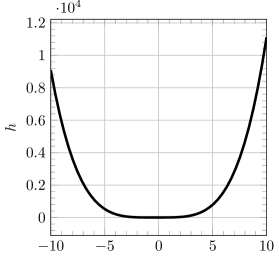
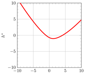
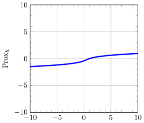
Figure 1: A visualization of Example 4.4. Depicted are $h$ (left), its conjugate $h^{*}$ (middle), and the proximal mapping $\operatorname{Prox}_{h}$ (right).

Example 4.5.

Suppose that

$$h(x)=\alpha x^{4},\quad\text{where $\alpha>0$,}$$ (53)

and let $y\in\mathbb{R}$. Then

$$h^{*}(y)=\frac{3}{4(4\alpha)^{1/3}}y^{4/3}$$ (54)

and

$$\operatorname{Prox}_{h}(y)=\frac{1}{2}\sqrt[3]{\frac{y}{\alpha}+\sqrt{\frac{1+27\alpha y^{2}}{27\alpha^{3}}}}+\frac{1}{2}\sqrt[3]{\frac{y}{\alpha}-\sqrt{\frac{1+27\alpha y^{2}}{27\alpha^{3}}}}.$$ (55)

Proof. Note that $h$ fits the pattern of 41 with $\beta=\gamma=\delta=\varepsilon=0$. The characterization of convexity presented in Proposition 4.1 turns into $\alpha>0$ and $0\geq 0$ which are both obviously true. Hence $h$ is convex.

We start by computing the Fenchel conjugate of $h$ using Proposition 4.2. We have $p=0$, $q=-y/(4\alpha)$, $\Delta=(y/(8\alpha))^{2}$, and $-\beta/(4\alpha)=0$. Hence $-q/2=y/(8\alpha)$ and $\sqrt{\Delta}=|y|/(8\alpha)$ which imply $\sqrt[3]{(-q/2)\pm\sqrt{\Delta}}=\sqrt[3]{y/(8\alpha)\pm|y|/(8\alpha)}=\sqrt[3]{\max\{0,y/(4\alpha)\}}$ or $\sqrt[3]{\min\{0,y/(4\alpha)\}}$. Using 46, we get

$$x_{y} =\sqrt[3]{\max\{0,y/(4\alpha)\}}+\sqrt[3]{\min\{0,y/(4\alpha)\}}=\sqrt[3]{y/(4\alpha)}.$$

Using Proposition 4.2, we obtain

$$h^{*}(y) =yx_{y}-h(x_{y})=yy^{1/3}/(4\alpha)^{1/3}-\alpha y^{4/3}/(4\alpha)^{4/3}$$

$$=\frac{|y|^{4/3}}{4^{1/3}\alpha^{1/3}}-\frac{|y|^{4/3}}{4^{4/3}\alpha^{1/3}}=\frac{|y|^{4/3}}{4^{1/3}\alpha^{1/3}}\big{(}1-\tfrac{1}{4}\big{)}=\frac{3|y|^{4/3}}{4(4\alpha)^{1/3}}$$

as claimed.

To compute $\operatorname{Prox}_{h}(y)$, we utilize Proposition 4.3. Obtain fresh values of $p,q,\Delta$, we have this time $p=1/(4\alpha)>0$ and $q=-y/(4\alpha)$ (see 49). Hence $\Delta=(p/3)^{3}+(q/2)^{2}=(1+27\alpha y^{2})/(1728\alpha^{3})$ and so $\sqrt{\Delta}=\sqrt{1+27\alpha y^{2}}/(8(3\alpha)^{3/2})$. Now $-\beta/(4\alpha)=0$ and $-q/2=y/(8\alpha)$, so 48 yields

$$\operatorname{Prox}_{h}(y) =\sqrt[3]{\frac{y}{8\alpha}+\frac{\sqrt{1+27\alpha y^{2}}}{8(3\alpha)^{3/2}}}+\sqrt[3]{\frac{y}{8\alpha}-\frac{\sqrt{1+27\alpha y^{2}}}{8(3\alpha)^{3/2}}}$$

$$=\frac{1}{2}\sqrt[3]{\frac{y}{\alpha}+\sqrt{\frac{1+27\alpha y^{2}}{27\alpha^{3}}}}+\frac{1}{2}\sqrt[3]{\frac{y}{\alpha}-\sqrt{\frac{1+27\alpha y^{2}}{27\alpha^{3}}}}$$

as claimed. $\hfill\quad\blacksquare$

Remark 4.6.

The Fenchel conjugate formula 54 is known and can also be computed by combining, e.g., [3, Example 13.2(i) with Proposition 13.23(i)]. The prox formula 55 appears — with a typo though — in [3, Example 24.38(v)]. Finally, for a Maple implementation for quartics, see [8].

5 The proximal mapping of $\alpha/x$

In this section, we study the convex reciprocal function

$$h(x):=\begin{cases}\alpha/x,&\text{if $x>0$;}\\ +\infty,&\text{if $x\leq 0$,}\end{cases}\qquad\text{where $\alpha>0$.}$$ (56)

The Fenchel conjugate $h^{*}$, which requires only solving a quadratic equation, is essentially known (e.g., combine [3, Example 13.2(ii) and Proposition 13.23(i)]), and given by

$$h^{*}(y)=\begin{cases}-2\sqrt{-\alpha y},&\text{if $y\leq 0$;}\\ +\infty,&\text{if $y>0$.}\end{cases}$$ (57)

The purpose of this section is to explicitly compute $\operatorname{Prox}_{h}$. We have the following result:

Proposition 5.1.

Suppose that $h$ is given by 56, and let $y\in\mathbb{R}$. Set $y_{0}:=-3\sqrt[3]{\alpha/4}\approx-1.88988\sqrt[3]{\alpha}$. Then we have the following three possibilities:

1. If $y_{0}<y$, then

   $$\operatorname{Prox}_{h}(y) =\frac{y}{3}+\sqrt[3]{\frac{\alpha}{2}+\Big{(}\frac{y}{3}\Big{)}^{3}+\sqrt{\alpha\Big{(}\frac{\alpha}{4}+\Big{(}\frac{y}{3}\Big{)}^{3}\Big{)}}}+\sqrt[3]{\frac{\alpha}{2}+\Big{(}\frac{y}{3}\Big{)}^{3}-\sqrt{\alpha\Big{(}\frac{\alpha}{4}+\Big{(}\frac{y}{3}\Big{)}^{3}\Big{)}}}.$$

2. If $y=y_{0}$, then

   $$\operatorname{Prox}_{h}(y_{0})=\sqrt[3]{\alpha}/\sqrt[3]{4}\approx 0.62996\sqrt[3]{\alpha}.$$

3. If $y<y_{0}$, then

   $$\operatorname{Prox}_{h}(y)=\frac{y}{3}\bigg{(}1-2\cos\Big{(}\frac{1}{3}\arccos\frac{(y/3)^{3}+\alpha/2}{-(y/3)^{3}}\Big{)}\bigg{)}.$$

Proof. Because $\operatorname{dom}h=\mathbb{R}_{++}$, we must find the positive solution of the equation $h^{\prime}(x)+x-y=0$. Since $h^{\prime}(x)=-\alpha x^{-2}$, we are looking for the (necessarily unique) positive solution of $x^{2}(h^{\prime}(x)+x-y)=0$, i.e., of

$$x^{3}-yx^{2}-\alpha=0.$$

This fits the pattern of 24 in Section 3, with parameters $a=1$, $b=-y$, $c=0$, and $d=-\alpha$. As in 27, we set We have

$$p :=\frac{3ac-b^{2}}{3a^{2}}=-\frac{y^{2}}{3}\begin{cases}<0,&\text{if $y\neq 0$;}\\ =0,&\text{if $y=0$}\end{cases}$$ (58)

and

$$q :=\frac{27a^{2}d+2b^{3}-9abc}{27a^{3}}=-\alpha-2(y/3)^{3}.$$

Next,

$$\Delta =(p/3)^{3}+(q/2)^{2}=-y^{6}/9^{3}+(\alpha+2(y/3)^{3})^{2}/4$$

$$=-(y/3)^{6}+\alpha^{2}/4+\alpha(y/3)^{3}+(y/3)^{6}$$

$$=\alpha\big{(}\alpha/4+(y/3)^{3}\big{)}.$$

Hence

$$\Delta\begin{cases}<0\Leftrightarrow y<y_{0};\\ =0\Leftrightarrow y=y_{0};\\ >0\Leftrightarrow y>y_{0},\end{cases}\quad\text{where}\;\;y_{0}:=-\frac{3}{\sqrt[3]{4}}\sqrt[3]{\alpha}\approx-1.88988\sqrt[3]{\alpha}.$$ (59)

Now set

$$x_{0}:=-\frac{b}{3a}=\frac{y}{3}.$$ (60)

Note that

$$-q/2=(y/3)^{3}+\alpha/2.$$ (61)

We now discuss the three possibilities from Corollary 3.2 — these will correspond to the three items of the result!

Case 1: $b^{2}=3ac$ or $\Delta>0$; equivalently, $y=0$ or $y>y_{0}$; equivalently, $y_{0}<y$.
Then Corollary 3.2(i) yields

$$\operatorname{Prox}_{h}(y) =x_{0}+\sqrt[3]{\frac{-q}{2}+\sqrt{\Delta}}+\sqrt[3]{\frac{-q}{2}-\sqrt{\Delta}}$$

$$=\frac{y}{3}+\sqrt[3]{\frac{\alpha}{2}+\Big{(}\frac{y}{3}\Big{)}^{3}+\sqrt{\alpha\Big{(}\frac{\alpha}{4}+\Big{(}\frac{y}{3}\Big{)}^{3}\Big{)}}}+\sqrt[3]{\frac{\alpha}{2}+\Big{(}\frac{y}{3}\Big{)}^{3}-\sqrt{\alpha\Big{(}\frac{\alpha}{4}+\Big{(}\frac{y}{3}\Big{)}^{3}\Big{)}}}$$

as claimed.

Case 2: $\Delta=0$; equivalently, $y=y_{0}$.
Then Corollary 3.2(ii) yields two distinct real roots. We can take a short cut here, though: By exploiting the continuity of $\operatorname{Prox}_{h}$ at $y_{0}$ via $\operatorname{Prox}_{h}(y_{0})=\lim_{y\to y_{0}^{+}}\operatorname{Prox}_{h}(y)$, we get

$$\operatorname{Prox}_{h}(y_{0})=\frac{y_{0}}{3}+2\sqrt[3]{\frac{\alpha}{2}+\Big{(}\frac{y_{0}}{3}\Big{)}^{3}}=\sqrt[3]{\alpha}/\sqrt[3]{4}\approx 0.62996\sqrt[3]{\alpha}.$$

Case 3: $\Delta<0$; equivalently, $y<y_{0}$.
By uniqueness of $\operatorname{Prox}_{h}(y)$, the desired root must be the largest (and the only positive) real root offered in this case (see Corollary 3.2(iii)):

$$\operatorname{Prox}_{h}(y)=x_{0}+2(-p/3)^{1/2}\cos\Big{(}\frac{\theta}{3}\Big{)},\quad\text{where}\;\;\theta:=\arccos\frac{-q/2}{(-p/3)^{3/2}},$$ (62)

By 58, $-p/3=y^{2}/9$; thus, using $y<y_{0}<0$, we have $(-p/3)^{1/2}=-y/3$, $(-p/3)^{3/2}=-(y/3)^{3}$, and 61 yields $-(q/2)/(-p/3)^{3/2}=-((y/3)^{3}+\alpha/2)/(y/3)^{3}$. This and 60 results in

$$\operatorname{Prox}_{h}(y)=\frac{y}{3}-2\frac{y}{3}\cos\Big{(}\frac{\theta}{3}\Big{)},\quad\text{where}\;\;\theta:=\arccos\bigg{(}-\frac{(y/3)^{3}+\alpha/2}{(y/3)^{3}}\bigg{)}.$$ (63)

$\hfill\quad\blacksquare$

Remark 5.2.

Suppose that $\alpha=1$. Then $\operatorname{Prox}_{h}$ was discussed in [9]; however, no explicit formulae were presented. For a visualization of $\operatorname{Prox}_{h}$ in this case, see Figure 2.

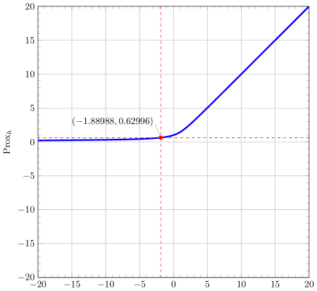
Figure 2: A visualization of Proposition 5.1 when $\alpha=1$.

6 Projection onto epigraph of a parabola

In this section, we study projection onto the epigraph of the function

$$h\colon\mathbb{R}^{n}\to\mathbb{R}\colon\mathbf{x}\mapsto\alpha\|\mathbf{x}\|^{2},\quad\text{where $\alpha>0$.}$$ (64)

Theorem 6.1.

Set $E:=\operatorname{epi}h\subseteq\mathbb{R}^{n+1}$. Let $(\mathbf{y},\eta)\in(\mathbb{R}^{n}\times\mathbb{R})$. If $(\mathbf{y},\eta)\in E$, then $P_{E}(\mathbf{y},\eta)=(\mathbf{y},\eta)$. So we assume that $(\mathbf{y},\eta)\in(\mathbb{R}^{n}\times\mathbb{R})\smallsetminus E$, i.e., $\alpha\|\mathbf{y}\|^{2}>\eta$. Set $\nu:=\|\mathbf{y}\|\geq 0$,

$$p:=-\frac{(2\alpha\eta-1)^{2}}{12\alpha^{2}},\quad q:=\frac{(2\alpha\eta-1)^{3}-27\alpha^{2}\nu^{2}}{108\alpha^{3}},$$ (65)

$\Delta:=(p/3)^{3}+(q/2)^{2}=(27\alpha^{2}{\nu^{2}}-2(2\alpha\eta-1)^{3})\nu^{2}/(1728\alpha^{4})$, and

$$x:=\begin{cases}-\dfrac{\alpha\eta+1}{3\alpha}+\sqrt[3]{-q/2+\sqrt{\Delta}}+\sqrt[3]{-q/2-\sqrt{\Delta}},&\text{if $\Delta\geq 0$;}\\[14.22636pt] -\dfrac{\alpha\eta+1}{3\alpha}+\dfrac{|2\alpha\eta-1|}{3\alpha}\cos\Big{(}\dfrac{1}{3}\arccos\dfrac{-q/2}{(-p/3)^{3/2}}\Big{)},&\text{if $\Delta<0$.}\end{cases}$$ (66)

Then

$$P_{E}(\mathbf{y},\eta)=\Big{(}\frac{\mathbf{y}}{1+2\alpha x},\eta+x\Big{)}.$$ (67)

See Figure 3 for an illustration for the case $\alpha=1/2$.

Proof. For $x\geq 0$, we have $xh=x\alpha\|\cdot\|^{2}$, $x\nabla h=2\alpha x\operatorname{Id}$, $\operatorname{Id}+x\nabla h=(1+2\alpha x)\operatorname{Id}$ and therefore $\operatorname{Prox}_{xh}=(1+2\alpha x)^{-1}\operatorname{Id}$. In view of [5, Theorem 6.36], we must first find a positive root $x$ of $\varphi(x):=h(\operatorname{Prox}_{xh}(\mathbf{y}))-x-\eta=\alpha\|\mathbf{y}\|^{2}/(1+2\alpha x)^{2}-x-\eta=0$. Note that $\varphi(0)>0$, that $\varphi$ is strictly decreasing on $\mathbb{R}_{+}$, and that $\varphi(x)\to-\infty$ as $x\to+\infty$. Hence $\varphi$ has exactly one positive root. Multiplying by $(1+2\alpha x)^{2}>0$, where $x>0$, results in the cubic $\alpha\nu^{2}-(x+\eta)(1+2\alpha x)^{2}=0$, which must have exactly one positive root. Re-arranging leads us to

$$f(x):=4\alpha^{2}x^{3}+4\alpha(\alpha\eta+1)x^{2}+(4\alpha\eta+1)x+\eta-\alpha\nu^{2}=0,$$ (68)

a cubic which we know has exactly one positive root. As in Section 3, we set

$$a:=4\alpha^{2},\;\;b:=4\alpha(\alpha\eta+1),\;\;c:=4\alpha\eta+1,\;\;d:=\eta-\alpha\nu^{2}<0,$$ (69)

$$p:=\frac{3ac-b^{2}}{3a^{2}}=-\frac{(2\alpha\eta-1)^{2}}{12\alpha^{2}}\leq 0,$$ (70)

and

$$q:=\frac{27a^{2}d+2b^{3}-9abc}{27a^{3}}=\frac{8\alpha^{3}\eta^{3}-12\alpha^{2}\eta^{2}+6\alpha\eta-27\alpha^{2}\nu^{2}-1}{108\alpha^{3}}.$$ (71)

We then have

$$\Delta :=(p/3)^{3}+(q/2)^{2}=\frac{\big{(}8\alpha^{3}\eta^{3}-12\alpha^{2}\eta^{2}+6\alpha\eta-27\alpha^{2}\nu^{2}-1\big{)}^{2}-(2\alpha\eta-1)^{6}}{(6\alpha)^{6}}$$ (72a)

$$=-\frac{\nu^{2}}{1728\alpha^{4}}\big{(}16\alpha^{3}\eta^{3}-24\alpha^{2}\eta^{2}+12\alpha\eta-27\alpha^{2}\nu^{2}-2\big{)}$$ (72b)

$$=\frac{\nu^{2}}{1728\alpha^{4}}\big{(}27\alpha^{2}\nu^{2}-2(2\alpha\eta-1)^{3}\big{)},$$ (72c)

as claimed. Utilizing Corollary 3.2, we have

$$x=-\frac{\alpha\eta+1}{3\alpha}+\sqrt[3]{-q/2+\sqrt{\Delta}}+\sqrt[3]{-q/2-\sqrt{\Delta}},\quad\text{if $\Delta\geq 0$}$$ (73a)

and

$$x=-\frac{\alpha\eta+1}{3\alpha}+\frac{|2\alpha\eta-1|}{3\alpha}\cos\Big{(}\frac{1}{3}\arccos\frac{-q/2}{(-p/3)^{3/2}}\Big{)}\quad\text{if $\Delta<0$.}$$ (73b)

(Because we know there is exactly one positive root, it is clear that we must pick $r_{0}$ in Corollary 3.2(iii) when $\Delta<0$.) Finally, [5, Theorem 6.36] yields

$$P_{E}(\mathbf{y},\eta)=\big{(}\operatorname{Prox}_{xh}(\mathbf{y}),\eta+x\big{)}=\Big{(}\frac{\mathbf{y}}{1+2\alpha x},\eta+x\Big{)}$$ (74)

as claimed. $\hfill\quad\blacksquare$

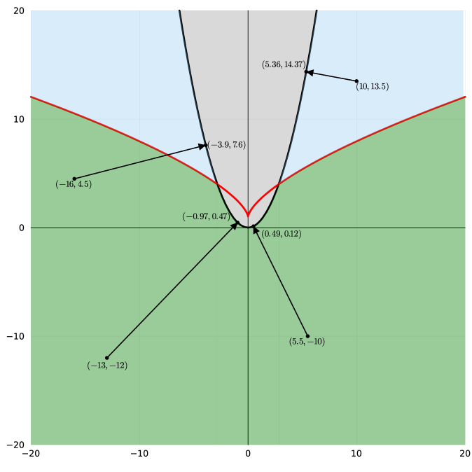
Figure 3: A visualization of Theorem 6.1 when $n=1$ and $\alpha=1/2$. The epigraph is shown in gray. The red curve corresponds to $\Delta=0$, the green region to $\Delta<0$ (where trig functions are used) and the blue region to $\Delta>0$.

7 On the projection of a rectangular hyperbolic paraboloid

In this section, $X$ is a real Hilbert space and we set

$$S:=\big{\{}{(\mathbf{x},\mathbf{y},\gamma)\in X\times X\times\mathbb{R}}~{}\big{|}~{}{\left\langle{\mathbf{x}},{\mathbf{y}}\right\rangle=\alpha\gamma}\big{\}},\quad\text{where $\alpha\in\mathbb{R}\smallsetminus\{0\}$.}$$ (75)

Using the Hilbert product space norm $\|(\mathbf{x},\mathbf{y},\gamma)\|:=\sqrt{\|\mathbf{x}\|^{2}+\|\mathbf{y}\|^{2}+\beta^{2}\gamma^{2}}$, where $\beta>0$, we are interested in finding the projection onto $S$. Various cases were discussed in [4], but 3 were treated only implicitly. Armed with the cubic, we are now able to treat two of these cases explicitly (the remaining case features a quintic and remains hard). The first case concerns

$$P_{S}(\mathbf{z},-\mathbf{z},\gamma),\quad\text{when}\;\;\mathbf{z}\in X\smallsetminus\{0\}\;\text{and}\;\alpha(\gamma-\alpha/\beta^{2})<-\|\mathbf{z}\|^{2}/4,$$ (76)

while the second case is

$$P_{S}(\mathbf{z},\mathbf{z},\gamma),\quad\text{when}\;\;\mathbf{z}\in X\smallsetminus\{0\}\;\text{and}\;\alpha(\gamma+\alpha/\beta^{2})>\|\mathbf{z}\|^{2}/4.$$ (77)

7.1 The case when 76 holds

Theorem 7.1.

Suppose $\mathbf{z}\in X\smallsetminus\{0\}$, set

$$\zeta:=\|\mathbf{z}\|>0,$$ (78)

and assume that

$$\alpha(\gamma-\alpha/\beta^{2})<-\zeta^{2}/4.$$ (79)

Set

$$p:=-\frac{(\alpha+\beta^{2}\gamma)^{2}}{3\alpha^{2}},\quad q:=\frac{2(\alpha+\beta^{2}\gamma)^{3}}{27\alpha^{3}}+\frac{\beta^{2}\zeta^{2}}{\alpha^{2}},$$ (80)

and

$$\Delta:=(p/3)^{3}+(q/2)^{2}=\frac{\beta^{2}\zeta^{2}}{\alpha^{2}}\Big{(}\frac{\beta^{2}\zeta^{2}}{4\alpha^{2}}+\frac{(\alpha+\beta^{2}\gamma)^{3}}{27\alpha^{3}}\Big{)}.$$ (81)

If $\Delta\geq 0$, then set

$$x:=\frac{2\alpha-\beta^{2}\gamma}{3\alpha}+\sqrt[3]{\frac{-q}{2}+\sqrt{\Delta}}+\sqrt[3]{\frac{-q}{2}-\sqrt{\Delta}};$$ (82)

and if $\Delta<0$, then set

$$x:=\frac{2\alpha-\beta^{2}\gamma}{3\alpha}+\delta\frac{2(\alpha+\beta^{2}\gamma)}{3\alpha}\cos\bigg{(}\frac{1}{3}\Big{(}(3+\delta)\pi+\arccos\frac{-q/2}{(-p/3)^{3/2}}\Big{)}\bigg{)}$$ (83a)

where

$$\delta:=\operatorname{sign}(\alpha^{2}+\alpha\beta^{2}\gamma)\in\{-1,0,1\}.$$ (83b)

Then $-1<x<1$ and

$$P_{S}(\mathbf{z},-\mathbf{z},\gamma)=\Big{(}\frac{\mathbf{z}}{1-x},\frac{-\mathbf{z}}{1-x},\gamma+\frac{\alpha x}{\beta^{2}}\Big{)}.$$ (84)

Proof. By [4, Theorem 4.1(ii)(a)], there exists a unique $x\in\left]-1,1\right[$ such that

$$\frac{2\zeta^{2}}{(1-x)^{2}}+\frac{2\alpha^{2}x}{\beta^{2}}+2\alpha\gamma=0;$$ (85)

multiplying by $\beta^{2}(1-x)^{2}/2>0$ yields the cubic

$$f(x):=ax^{3}+bx^{2}+cx+d=0$$ (86)

where

$$a:=\alpha^{2}>0,\;\;b:=\alpha\beta^{2}\gamma-2\alpha^{2},\;\;c:=\alpha^{2}-2\alpha\beta^{2}\gamma,\;\;d:=\alpha\beta^{2}\gamma+\beta^{2}\zeta^{2}.$$ (87)

Our strategy is to systematically discuss all cases of Theorem 3.1 and then combine cases as much as possible. As usual, we set

$$x_{0}:=-\frac{b}{3a}=\frac{2\alpha-\beta^{2}\gamma}{3\alpha}=\frac{2\alpha^{2}-\alpha\beta^{2}\gamma}{3\alpha^{2}}\quad\text{and}\quad p:=\frac{3ac-b^{2}}{3a^{2}}=-\frac{(\alpha+\beta^{2}\gamma)^{2}}{3\alpha^{2}}\leq 0,$$ (88)

and we note that the definition of $p$ is consistent with the one given in 80. We have the characterization

$$p=0\;\Leftrightarrow\;\alpha+\beta^{2}\gamma=0\;\Leftrightarrow\;\gamma=-\alpha/\beta^{2}.$$ (89)

Again as usual, we set

$$q:=\frac{27a^{2}d+2b^{2}-9abc}{27a^{3}}=\frac{2(\alpha+\beta^{2}\gamma)^{3}}{27\alpha^{3}}+\frac{\beta^{2}\zeta^{2}}{\alpha^{2}},$$ (90)

which matches 80, and of course

$$\Delta:=(p/3)^{3}+(q/2)^{2}=\frac{\beta^{2}\zeta^{2}}{\alpha^{2}}\Big{(}\frac{\beta^{2}\zeta^{2}}{4\alpha^{2}}+\frac{(\alpha+\beta^{2}\gamma)^{3}}{27\alpha^{3}}\Big{)},$$ (91)

which matches 81. We now systematically discuss the case of Theorem 3.1.

Case 1: $p<0$, i.e., $\alpha+\beta^{2}\gamma\neq 0$ by 80.

Case 1(a): $p<0$ and $\Delta>0$.
Then Theorem 3.1(i)(a) and the definition $x_{0}$ in 88 yield 82.

Case 1(b): $p<0$ and $\Delta=0$.
By Theorem 3.1(i)(b), there are two roots, $x_{0}+3q/p$ and $x_{0}-3q/(2p)$, one of which lies in $\left]-1,1\right[$. Now

$$x_{0}-\frac{3q}{2p}-1 =\frac{2\alpha-\beta^{2}\gamma}{3\alpha}-\frac{3}{2}\frac{2(\alpha+\beta^{2}\gamma)^{3}+27\alpha\beta^{2}\zeta^{2}}{27\alpha^{3}}\frac{-3\alpha^{2}}{(\alpha+\beta^{2}\gamma)^{2}}-1$$

$$=\frac{2\alpha-\beta^{2}\gamma}{3\alpha}+\frac{(\alpha+\beta^{2}\gamma)^{3}+27\alpha\beta^{2}\zeta^{2}/2}{3\alpha(\alpha+\beta^{2}\gamma)^{2}}-1$$

$$=\frac{\big{(}(2\alpha-\beta^{2}\gamma)+(\alpha+\beta^{2}\gamma)-(3\alpha)\big{)}}{3\alpha(\alpha+\beta^{2}\gamma)^{2}}(\alpha+\beta^{2}\gamma)^{2}+\frac{27\alpha\beta^{2}\zeta^{2}/2}{3\alpha(\alpha+\beta^{2}\gamma)^{2}}$$

$$=\frac{9\beta^{2}\zeta^{2}}{2(\alpha+\beta^{2}\gamma)^{2}}$$

$$\geq 0;$$

hence the root $x_{0}-3q/(2p)$ lies in $\left[1,+\infty\right[$ and therefore our desired root is the remaining one, namely $x_{0}+3q/p$, which also allows us to use the representation 82.

Case 1(c): $p<0$ and $\Delta<0$.
According to Theorem 3.1(i)(c), we have three distinct real roots, but there is information about their location. We must locate the root in $\left]-1,1\right[$. First, $b^{2}-3ac=(\alpha^{2}+\alpha\beta^{2}\gamma)^{2}$ which yields $\sqrt{b^{2}-3ac}=|\alpha^{2}+\alpha\beta^{2}\gamma|$. This and the definition of $b$ yields

$$x_{\pm} :=\frac{-b\pm\sqrt{b^{2}-3ac}}{3a}=\frac{2\alpha^{2}-\alpha\beta^{2}\gamma\pm|\alpha^{2}+\alpha\beta^{2}\gamma|}{3\alpha^{2}}$$

$$=\frac{1}{3\alpha^{2}}\frac{(3\alpha^{2})+(\alpha^{2}-2\alpha\beta^{2}\gamma)\pm\big{|}(3\alpha^{2})-(\alpha^{2}-2\alpha\beta^{2}\gamma)\big{|}}{2}.$$

Hence

$$x_{-}=\frac{\min\{3\alpha^{2},\alpha^{2}-2\alpha\beta^{2}\gamma\}}{3\alpha^{2}}<\frac{\max\{3\alpha^{2},\alpha^{2}-2\alpha\beta^{2}\gamma\}}{3\alpha^{2}}=x_{+}.$$ (92)

We now bifurcate one last time.

Case 1(c)($+$): $p<0$, $\Delta<0$, and $\alpha^{2}+\alpha\beta^{2}\gamma>0$.
Then $3\alpha^{2}>\alpha^{2}-2\alpha\beta^{2}\gamma$ and therefore $x_{+}=1$. It follows that our desired root $x$ is the “middle root” corresponding to $k=2$ in Theorem 3.1(i)(c):

$$x =x_{0}+2(-p/3)^{1/2}\cos\bigg{(}\frac{1}{3}\Big{(}4\pi+\arccos\frac{-q/2}{(-p/3)^{3/2}}\Big{)}\bigg{)}$$

$$=\frac{2\alpha-\beta^{2}\gamma}{3\alpha}+\frac{2|\alpha+\beta^{2}\gamma|}{3|\alpha|}\cos\bigg{(}\frac{1}{3}\Big{(}4\pi+\arccos\frac{-q/2}{(-p/3)^{3/2}}\Big{)}\bigg{)}$$

$$=\frac{2\alpha-\beta^{2}\gamma}{3\alpha}+\frac{2(\alpha+\beta^{2}\gamma)}{3\alpha}\cos\bigg{(}\frac{1}{3}\Big{(}4\pi+\arccos\frac{-q/2}{(-p/3)^{3/2}}\Big{)}\bigg{)},$$

where in the last line we used the assumption to deduce that $|\alpha+\beta^{2}\gamma|/|\alpha|=|\alpha^{2}+\alpha\beta^{2}\gamma|/\alpha^{2}=(\alpha^{2}+\alpha\beta^{2}\gamma)/\alpha^{2}=(\alpha+\beta^{2}\gamma)/\alpha$.

Case 1(c)($-$): $p<0$, $\Delta<0$, and $\alpha^{2}+\alpha\beta^{2}\gamma\leq 0$.
Then $3\alpha^{2}\leq\alpha^{2}-2\alpha\beta^{2}\gamma$ and therefore $x_{-}=1$. It follows that our desired root is the “smallest root” corresponding to $k=1$ in Theorem 3.1(i)(c):

$$x =x_{0}+2(-p/3)^{1/2}\cos\bigg{(}\frac{1}{3}\Big{(}2\pi+\arccos\frac{-q/2}{(-p/3)^{3/2}}\Big{)}\bigg{)}$$

$$=\frac{2\alpha-\beta^{2}\gamma}{3\alpha}+\frac{2|\alpha+\beta^{2}\gamma|}{3|\alpha|}\cos\bigg{(}\frac{1}{3}\Big{(}2\pi+\arccos\frac{-q/2}{(-p/3)^{3/2}}\Big{)}\bigg{)}$$

$$=\frac{2\alpha-\beta^{2}\gamma}{3\alpha}-\frac{2(\alpha+\beta^{2}\gamma)}{3\alpha}\cos\bigg{(}\frac{1}{3}\Big{(}2\pi+\arccos\frac{-q/2}{(-p/3)^{3/2}}\Big{)}\bigg{)},$$

where in the last line we used the assumption to deduce that $|\alpha+\beta^{2}\gamma|/|\alpha|=|\alpha^{2}+\alpha\beta^{2}\gamma|/\alpha^{2}=-(\alpha^{2}+\alpha\beta^{2}\gamma)/\alpha^{2}=-(\alpha+\beta^{2}\gamma)/\alpha$.

Note that the last two cases can be combined to obtain 83.

Case 2: $p=0$, i.e., $\alpha+\beta^{2}\gamma=0$ by 80. Then $\Delta=(q/2)^{2}\geq 0$; hence, $\sqrt{\Delta}=|q|/2$ and thus $\{-q/2\pm\sqrt{\Delta}\}=\{-q,0\}$. By Theorem 3.1(ii), the only real root is $x_{0}+(-q)^{1/3}=x_{0}+(-q/2+\sqrt{\Delta})^{1/3}+(-q/2-\sqrt{\Delta})^{1/3}$ which is the same as 82 using 88.

Case 3: $p>0$. In vie of 80, this case never occurs. $\hfill\quad\blacksquare$

7.2 The case when 77 holds

Theorem 7.2.

Suppose $\mathbf{z}\in X\smallsetminus\{0\}$, set

$$\zeta:=\|\mathbf{z}\|>0,$$ (93)

and assume that

$$\alpha(\gamma+\alpha/\beta^{2})>\zeta^{2}/4.$$ (94)

Set

$$p:=-\frac{(\beta^{2}\gamma-\alpha)^{2}}{3\alpha^{2}},\quad q:=\frac{2(\beta^{2}\gamma-\alpha)^{3}}{27\alpha^{3}}-\frac{\beta^{2}\zeta^{2}}{\alpha^{2}},$$ (95)

and

$$\Delta:=(p/3)^{3}+(q/2)^{2}=\frac{\beta^{2}\zeta^{2}}{\alpha^{2}}\Big{(}\frac{\beta^{2}\zeta^{2}}{4\alpha^{2}}-\frac{(\beta^{2}\gamma-\alpha)^{3}}{27\alpha^{3}}\Big{)}.$$ (96)

If $\Delta\geq 0$, then set

$$x:=-\frac{2\alpha+\beta^{2}\gamma}{3\alpha}+\sqrt[3]{\frac{-q}{2}+\sqrt{\Delta}}+\sqrt[3]{\frac{-q}{2}-\sqrt{\Delta}};$$ (97)

and if $\Delta<0$, then set

$$x:=-\frac{2\alpha+\beta^{2}\gamma}{3\alpha}+\delta\frac{2(\alpha-\beta^{2}\gamma)}{3\alpha}\cos\bigg{(}\frac{1}{3}\Big{(}(2+2\delta)\pi+\arccos\frac{-q/2}{(-p/3)^{3/2}}\Big{)}\bigg{)}$$ (98a)

where

$$\delta:=\operatorname{sign}(\alpha^{2}-\alpha\beta^{2}\gamma)\in\{-1,0,1\}.$$ (98b)

Then $-1<x<1$ and

$$P_{S}(\mathbf{z},\mathbf{z},\gamma)=\Big{(}\frac{\mathbf{z}}{1+x},\frac{\mathbf{z}}{1+x},\gamma+\frac{\alpha x}{\beta^{2}}\Big{)}.$$ (99)

Proof. By [4, Theorem 4.1(iii)(a)], there exists a unique $x\in\left]-1,1\right[$ such that

$$\frac{2\zeta^{2}}{(1+x)^{2}}-\frac{2\alpha^{2}x}{\beta^{2}}-2\alpha\gamma=0;$$ (100)

multiplying by $-\beta^{2}(1+x)^{2}/2<0$ yields the cubic

$$f(x):=ax^{3}+bx^{2}+cx+d=0$$ (101)

where

$$a:=\alpha^{2}>0,\;\;b:=\alpha\beta^{2}\gamma+2\alpha^{2},\;\;c:=\alpha^{2}+2\alpha\beta^{2}\gamma,\;\;d:=\alpha\beta^{2}\gamma-\beta^{2}\zeta^{2}.$$ (102)

Our strategy is to systematically discuss all cases of Theorem 3.1 and then combine cases as much as possible. As usual, we set

$$x_{0}:=-\frac{b}{3a}=-\frac{2\alpha+\beta^{2}\gamma}{3\alpha}=-\frac{2\alpha^{2}+\alpha\beta^{2}\gamma}{3\alpha^{2}}\quad\text{and}\quad p:=\frac{3ac-b^{2}}{3a^{2}}=-\frac{(\beta^{2}\gamma-\alpha)^{2}}{3\alpha^{2}}\leq 0,$$ (103)

and we note that the definition of $p$ is consistent with the one given in 95. We have the characterization

$$p=0\;\Leftrightarrow\;\beta^{2}\gamma-\alpha=0\;\Leftrightarrow\;\gamma=\alpha/\beta^{2}.$$ (104)

Again as usual, we set

$$q:=\frac{27a^{2}d+2b^{2}-9abc}{27a^{3}}=\frac{2(\beta^{2}\gamma-\alpha)^{3}}{27\alpha^{3}}-\frac{\beta^{2}\zeta^{2}}{\alpha^{2}},$$ (105)

which matches 95, and of course

$$\Delta:=(p/3)^{3}+(q/2)^{2}=\frac{\beta^{2}\zeta^{2}}{\alpha^{2}}\Big{(}\frac{\beta^{2}\zeta^{2}}{4\alpha^{2}}-\frac{(\beta^{2}\gamma-\alpha)^{3}}{27\alpha^{3}}\Big{)},$$ (106)

which matches 96. We now systematically discuss the case of Theorem 3.1.

Case 1: $p<0$, i.e., $\beta^{2}\gamma-\alpha\neq 0$ by 95.

Case 1(a): $p<0$ and $\Delta>0$.
Then Theorem 3.1(i)(a) and the definition of $x_{0}$ in 103 yield 97.

Case 1(b): $p<0$ and $\Delta=0$.
By Theorem 3.1(i)(b), there are two roots, $x_{0}+3q/p$ and $x_{0}-3q/(2p)$, one of which lies in $\left]-1,1\right[$. Now

$$x_{0}-\frac{3q}{2p}+1 =-\frac{2\alpha+\beta^{2}\gamma}{3\alpha}-\frac{3}{2}\frac{2(\beta^{2}\gamma-\alpha)^{3}-27\alpha\beta^{2}\zeta^{2}}{27\alpha^{3}}\frac{-3\alpha^{2}}{(\beta^{2}\gamma-\alpha)^{2}}+1$$

$$=-\frac{2\alpha+\beta^{2}\gamma}{3\alpha}+\frac{(\beta^{2}\gamma-\alpha)^{3}-27\alpha\beta^{2}\zeta^{2}/2}{3\alpha(\beta^{2}\gamma-\alpha)^{2}}+1$$

$$=\frac{\big{(}(-2\alpha-\beta^{2}\gamma)+(\beta^{2}\gamma-\alpha)+(3\alpha)\big{)}}{3\alpha(\beta^{2}\gamma-\alpha)^{2}}(\beta^{2}\gamma-\alpha)^{2}-\frac{27\alpha\beta^{2}\zeta^{2}/2}{3\alpha(\beta^{2}\gamma-\alpha)^{2}}$$

$$=-\frac{9\beta^{2}\zeta^{2}}{2(\beta^{2}\gamma-\alpha)^{2}}$$

$$\leq 0;$$

hence the root $x_{0}-3q/(2p)$ lies in $\left]-\infty,-1\right]$ and therefore our desired root is the remaining one, namely $x_{0}+3q/p$, which also allows us to use the representation 97.

Case 1(c): $p<0$ and $\Delta<0$.
According to Theorem 3.1(i)(c), we have three distinct real roots, but there is information about their location. We must locate the root in $\left]-1,1\right[$. First, $b^{2}-3ac=(\alpha^{2}-\alpha\beta^{2}\gamma)^{2}$ which yields $\sqrt{b^{2}-3ac}=|\alpha^{2}-\alpha\beta^{2}\gamma|$. This and the definition of $b$ yields

$$x_{\pm} :=\frac{-b\pm\sqrt{b^{2}-3ac}}{3a}=\frac{-2\alpha^{2}-\alpha\beta^{2}\gamma\pm|\alpha^{2}-\alpha\beta^{2}\gamma|}{3\alpha^{2}}$$

$$=\frac{1}{3\alpha^{2}}\frac{(-3\alpha^{2})+(-\alpha^{2}-2\alpha\beta^{2}\gamma)\pm\big{|}(-3\alpha^{2})-(-\alpha^{2}-2\alpha\beta^{2}\gamma)\big{|}}{2}.$$

Hence

$$x_{-}=\frac{\min\{-3\alpha^{2},-\alpha^{2}-2\alpha\beta^{2}\gamma\}}{3\alpha^{2}}<\frac{\max\{-3\alpha^{2},-\alpha^{2}-2\alpha\beta^{2}\gamma\}}{3\alpha^{2}}=x_{+}.$$ (107)

We now bifurcate one last time.

Case 1(c)($+$): $p<0$, $\Delta<0$, and $\alpha^{2}-\alpha\beta^{2}\gamma>0$.
Then $-3\alpha^{2}<-\alpha^{2}-2\alpha\beta^{2}\gamma$ and therefore $x_{-}=-1$. It follows that our desired root $x$ is the “middle root” corresponding to $k=2$ in Theorem 3.1(i)(c):

$$x =x_{0}+2(-p/3)^{1/2}\cos\bigg{(}\frac{1}{3}\Big{(}4\pi+\arccos\frac{-q/2}{(-p/3)^{3/2}}\Big{)}\bigg{)}$$

$$=-\frac{2\alpha+\beta^{2}\gamma}{3\alpha}+\frac{2|\beta^{2}\gamma-\alpha|}{3|\alpha|}\cos\bigg{(}\frac{1}{3}\Big{(}4\pi+\arccos\frac{-q/2}{(-p/3)^{3/2}}\Big{)}\bigg{)}$$

$$=-\frac{2\alpha+\beta^{2}\gamma}{3\alpha}+\frac{2(\alpha-\beta^{2}\gamma)}{3\alpha}\cos\bigg{(}\frac{1}{3}\Big{(}4\pi+\arccos\frac{-q/2}{(-p/3)^{3/2}}\Big{)}\bigg{)},$$

where in the last line we used the assumption to deduce that $|\beta^{2}\gamma-\alpha|/|\alpha|=|\alpha\beta^{2}\gamma-\alpha^{2}|/\alpha^{2}=(\alpha^{2}-\alpha\beta^{2}\gamma)/\alpha^{2}=(\alpha-\beta^{2}\gamma)/\alpha$.

Case 1(c)($-$): $p<0$, $\Delta<0$, and $\alpha^{2}-\alpha\beta^{2}\gamma\leq 0$.
Then $-3\alpha^{2}\geq-\alpha^{2}-2\alpha\beta^{2}\gamma$ and therefore $x_{+}=-1$. It follows that our desired root is the “largest root” corresponding to $k=0$ in Theorem 3.1(i)(c):

$$x =x_{0}+2(-p/3)^{1/2}\cos\bigg{(}\frac{1}{3}\Big{(}\arccos\frac{-q/2}{(-p/3)^{3/2}}\Big{)}\bigg{)}$$

$$=-\frac{2\alpha+\beta^{2}\gamma}{3\alpha}+\frac{2|\beta^{2}\gamma-\alpha|}{3|\alpha|}\cos\bigg{(}\frac{1}{3}\Big{(}\arccos\frac{-q/2}{(-p/3)^{3/2}}\Big{)}\bigg{)}$$

$$=-\frac{2\alpha+\beta^{2}\gamma}{3\alpha}+\frac{2(\beta^{2}\gamma-\alpha)}{3\alpha}\cos\bigg{(}\frac{1}{3}\Big{(}\arccos\frac{-q/2}{(-p/3)^{3/2}}\Big{)}\bigg{)},$$

where in the last line we used the assumption to deduce that $|\beta^{2}\gamma-\alpha|/|\alpha|=|\alpha\beta^{2}\gamma-\alpha^{2}|/\alpha^{2}=(\alpha\beta^{2}\gamma-\alpha^{2})/\alpha^{2}=(\beta^{2}\gamma-\alpha)/\alpha$.

Note that the last two cases can be combined to obtain 98.

Case 2: $p=0$, i.e., $\alpha-\beta^{2}\gamma=0$ by 95. Then $\Delta=(q/2)^{2}\geq 0$; hence, $\sqrt{\Delta}=|q|/2$ and thus $\{-q/2\pm\sqrt{\Delta}\}=\{-q,0\}$. By Theorem 3.1(ii), the only real root is $x_{0}+(-q)^{1/3}=x_{0}+(-q/2+\sqrt{\Delta})^{1/3}+(-q/2-\sqrt{\Delta})^{1/3}$ which is the same as 97 using 103.

Case 3: $p>0$. In view of 95, this case never occurs. $\hfill\quad\blacksquare$

8 A proximal mapping of a closure of a perspective function

The following completes [3, Example 24.57] which stopped short of providing solutions for a cubic encountered.

Example 8.1.

Define the function $h$ on $\mathbb{R}^{n}\times\mathbb{R}$ by

$$h(y,\eta):=\begin{cases}\|y\|^{2}/(2\eta),&\text{if $\eta>0$;}\\ 0,&\text{if $y=0$ and $\eta=0$;}\\ +\infty,&\text{otherwise.}\end{cases}$$ (108)

Let $\gamma>0$ and $(y,\eta)\in\mathbb{R}^{n}\times\mathbb{R}$. Then

$$\operatorname{Prox}_{\gamma h}(y,\eta)=\begin{cases}(0,0),&\text{if $\|y\|^{2}+2\gamma\eta\leq 0$;}\\ \Big{(}\big{(}1-\frac{\gamma\lambda}{\|y\|}\big{)}y,\eta+\frac{\gamma\lambda^{2}}{2}\Big{)},&\text{if $\|y\|^{2}+2\gamma\eta>0$,}\end{cases}$$ (109)

where $p=2(\eta+\gamma)/\gamma$, $\Delta=(p/3)^{3}+(\|y\|/\gamma)^{2}$, and

$$\lambda=\begin{cases}\sqrt[3]{\dfrac{\|y\|}{\gamma}+\sqrt{\Delta}}+\sqrt[3]{\dfrac{\|y\|}{\gamma}-\sqrt{\Delta}},&\text{if $\Delta\geq 0$;}\\[19.91692pt] 2(-p/3)^{1/2}\cos\Big{(}\dfrac{1}{3}\arccos\dfrac{\|y\|/\gamma}{(-p/3)^{3/2}}\Big{)},&\text{if $\Delta<0$.}\end{cases}$$ (110)

Proof. The first cases where already provided in [3, Example 24.57]. Now assume $\|y\|^{2}+2\gamma\eta>0$. It was also observed in [3, Example 24.57] that if $y=0$, then $\operatorname{Prox}_{\gamma h}(y,\eta)=(0,\eta)$.

So assume also that $y\neq 0$. It follows from the discussion that in [3, Example 24.57] that $\lambda$ is the unique positive solution of the already depressed cubic

$$\lambda^{3}+\frac{2(\eta+\gamma)}{\gamma}\lambda-\frac{2\|y\|}{\gamma}=0,$$ (111)

which is where the discussion in [3] halted. Continuing here, we set

$$p:=\frac{2(\eta+\gamma)}{\gamma},\quad q:=-\frac{2\|y\|}{\gamma}<0,$$ (112)

and $\Delta:=(p/3)^{3}+(q/2)^{2}$. Using Corollary 2.2, we see that if $\Delta<0$, then

$$\lambda=2(-p/3)^{1/2}\cos\Big{(}\frac{1}{3}\arccos\frac{-q/2}{(-p/3)^{3/2}}\Big{)}$$ (113)

while if $\Delta\geq 0$, then

$$\lambda=\sqrt[3]{\frac{-q}{2}+\sqrt{\Delta}}+\sqrt[3]{\frac{-q}{2}-\sqrt{\Delta}}$$ (114)

which slightly simplifies to the expression provided in 110.

Finally, notice that if $y=0$, then the assumption that $\|y\|^{2}+2\gamma\eta>0$ yields $\eta>0$; thus, $p>0$, $q=0$, and hence $\Delta>0$. Formally, our $\lambda$ then simplifies to $0$ which conveniently allows us to combine this case with the case $y\neq 0$. $\hfill\quad\blacksquare$

References

[1]
[2] M. Abramowitz and I. A. Stegun,
Handbook of Mathematical Functions,
Dover, 1965.
[3]
H.H. Bauschke, and P.L. Combettes,
Convex Analysis and Monotone Operator Theory in Hilbert Spaces,
second edition,
Springer, 2017.
[4]
H.H. Bauschke, M. Krishan Lal, and X. Wang, Projections onto rectangular hyperbolic paraboloids in Hilbert spaces, Applied Set-Valued Analysis and Optimization, accepted, (2022). https://arxiv.org/abs/2206.04878
[5] A. Beck,
First-Order Methods in Optimization,
SIAM, 2017.
[6] G. Blekherman, P.A. Parillo, and R.R. Thomas (editors),
Semidefinite Optimization and Convex Algebraic Geometry,
SIAM, 2013.
[7]
S. Confalonieri,
The Unattainable Attempt to Avoid the Casus Irreducibilis for Cubic Equations, Springer, 2015.