Abstract

Gradient boosting machines (GBMs) based on decision trees consistently demonstrate state-of-the-art results on regression and classification tasks with tabular data, often outperforming deep neural networks. However, these models do not provide well-calibrated predictive uncertainties, which prevents their use for decision making in high-risk applications. The Bayesian treatment is known to improve predictive uncertainty calibration, but previously proposed Bayesian GBM methods are either computationally expensive, or resort to crude approximations. Variational inference is often used to implement Bayesian neural networks, but is difficult to apply to GBMs, because the decision trees used as weak learners are non-differentiable. In this paper, we propose to implement Bayesian GBMs using variational inference with soft decision trees, a fully differentiable alternative to standard decision trees introduced by Irsoy et al., Our experiments demonstrate that variational soft trees and variational soft GBMs provide useful uncertainty estimates, while retaining good predictive performance. The proposed models show higher test likelihoods when compared to the state-of-the-art Bayesian GBMs in 7/10 tabular regression datasets and improved out-of-distribution detection in 5/10 datasets.

1 INTRODUCTION

Tabular data, often combining both real valued and categorical variables, is common in machine learning applications (Borisov et al.,, 2021; Hoang and Wiegratz,, 2021; Clements et al.,, 2020; Ebbehoj et al.,, 2021; Mustafa and Rahimi Azghadi,, 2021). A number of these applications require uncertainty estimates, in addition to the model’s predictions. Predictive uncertainty is particularly important when using the model for making decisions associated with risk, as common in healthcare (Abdullah et al.,, 2022; Kompa et al.,, 2021) or finance (Bew et al.,, 2019; Gonzalvez et al.,, 2019). In order to make optimal decisions, we require the uncertainty estimates to be well-calibrated: the predictive distribution returned by the model should capture the true likelihood of the targets (Guo et al.,, 2017).

A decision tree is a predictive model that is fit by recursively partitioning the feature space. These models are fast, interpretable and support categorical data without additional pre-processing. To increase their expressivity without exacerbating overfitting, multiple decision trees can be combined into an ensemble using gradient boosting (Freund and Schapire,, 1997; Friedman,, 2001). Gradient boosting machines (GBM) are an expressive class of machine learning models trained by sequentially fitting an ensemble of weak learners (e.g. decision trees). At each iteration, the gradient boosting procedure fits an additional weak learner that would minimize the training error when added to the ensemble. These models demonstrate state-of-the-art results on tabular data (Bojer and Meldgaard,, 2021; Liu et al.,, 2021), often out-performing deep neural networks (Borisov et al.,, 2021; Shwartz-Ziv and Armon,, 2022).

While GBM models demonstrate good predictive performance, they do not provide well-calibrated predictive uncertainties (Niculescu-Mizil and Caruana,, 2012). Bayesian methods are known to improve predictive uncertainties by explicitly capturing the epistemic uncertainty, a type of uncertainty that results from learning with finite data (Kristiadi et al.,, 2020; Mitros and Namee,, 2019). Bayesian GBMs have been proposed, and indeed improve upon the predictive uncertainties of standard GBMs (Chipman et al.,, 1998; Linero and Yang,, 2017; Ustimenko and Prokhorenkova,, 2020). Current methods rely on Markov chain Monte Carlo (MCMC) to sample from the posterior, however, and do not scale well to larger models and datasets. Alternative approximate sampling methods have been proposed by He and Hahn, (2020) and Malinin et al., (2020). These methods make the sampling procedure more efficient, but degrade the quality of the resulting predictive uncertainties. More scalable approximate inference methods such as the Laplace approximation or variational inference are difficult to apply to GBMs, because the decision trees used as weak learners are non-differentiable.

Unlike standard decision trees that route the input to a unique leaf based on a series of binary conditions, soft decision trees (Irsoy et al.,, 2012) compute a convex combination of all leaves, weighing their values by a series of learned gating functions. As a result, soft decision trees are fully differentiable, and therefore amenable to scalable Bayesian inference methods that are common in Bayesian deep learning (Blundell et al.,, 2015; Cobb and Jalaian,, 2020; Immer et al.,, 2020).

In this work we propose to implement Bayesian GBMs by using soft trees as week learners in a GBM, and performing variational inference on the resulting model. In particular, we make the following contributions:

1. We propose a method for performing variational inference in soft decision trees. The chosen variational distribution allows trading-off memory and computation for a richer posterior approximation.

2. We increase the expressivity of the model by using variational soft trees as weak learners in a GBM.

3. We run experiments to demonstrate that the proposed models perform well on tabular data, yielding useful predictive uncertainties in regression, out-of-distribution detection and contextual bandits.

2 BACKGROUND

2.1 Bayesian inference

Bayesian inference provides a theoretical framework for reasoning about model uncertainty, and has been shown to improve calibration of machine learning models in practice (Mitros and Namee,, 2019; Kristiadi et al.,, 2020). In Bayesian inference we place a prior on the model parameters $\theta$, and use the Bayes rule to define the posterior distribution having observed the data:

$$p\mathopen{}\left(\theta\,|\,\mathcal{D}\right)\mathclose{}\propto p\mathopen{}\left(\mathcal{D}\,|\,\theta\right)\mathclose{}p\mathopen{}\left(\theta\right)\mathclose{}$$ (1)

where $\mathcal{D}=\left\{x_{i},y_{i}\right\}_{i=1}^{n}$ is the training data, $p\mathopen{}\left(\theta\right)\mathclose{}$ is the prior distribution, and $p\mathopen{}\left(\mathcal{D}\,|\,\theta\right)\mathclose{}$ the likelihood. The predictive distribution of a new target $y^{*}$ given a feature vector $x^{*}$ is then computed as

$$p\mathopen{}\left(y^{*}\,|\,x^{*}\right)\mathclose{}={\mathop{{}\mathbb{E}}}_{\theta\sim p\mathopen{}\left(\theta\,|\,\mathcal{D}\right)\mathclose{}}\mathopen{}\left[p\mathopen{}\left(y^{*}\,|\,x^{*},\theta\right)\mathclose{}\right]\mathclose{}$$ (2)

The posterior distribution in the Bayesian paradigm explicitly captures epistemic or model uncertainty that results from learning with finite data. Epistemic uncertainty is one of the two fundamental types of uncertainty (alongside the aleatoric or data uncertainty), and capturing it was shown to be especially important in risk-aware decision making (Riquelme et al.,, 2018; Abdullah et al.,, 2022; Deisenroth and Rasmussen,, 2011), active learning (Kirsch et al.,, 2019) and Bayesian optimisation (Gonzalvez et al.,, 2019; Krause et al.,, 2006; Springenberg et al.,, 2016). Unfortunately, the posterior distribution is typically intractable and requires numerical approximation.

Variational inference

Variational inference (VI) is an approximate inference method which selects a distribution $q^{*}$ within a variational family $\mathcal{Q}$ that best approximates the posterior $p$. More formally, we select the distribution $q^{*}$ such that:

$$q^{*} =\operatorname*{\arg\!\min}_{q\in\mathcal{Q}}D_{\mathrm{KL}}\mathopen{}\left(q\,\|\,p\right)\mathclose{}$$ (3)

$$=\operatorname*{\arg\!\min}_{q\in\mathcal{Q}}{\mathop{{}\mathbb{E}}}_{\theta\sim q}\mathopen{}\left[\log\frac{q\mathopen{}\left(\theta\right)\mathclose{}}{p\mathopen{}\left(\theta\,|\,\mathcal{D}\right)\mathclose{}}\right]\mathclose{}.$$

In practice, we define a parametric variational distribution $q_{\phi}$ and use standard optimization methods like stochastic gradient descent to minimize the KL loss w.r.t. $\phi$. We then use $q^{*}\mathopen{}\left(\theta\right)\mathclose{}$ instead of $p\mathopen{}\left(\theta\,|\,\mathcal{D}\right)\mathclose{}$ to approximate the predictive distribution in Equation 2. In this paper, we focus on VI because it can capture arbitrarily complex, high-dimensional posteriors, assuming the chosen variational family is sufficiently expressive. At the same time, VI can scale to large datasets when combined with stochastic optimisation (Hoffman et al.,, 2013; Swiatkowski et al.,, 2020; Tomczak et al.,, 2020; Tran et al.,, 2015).

Other commonly used approximate inference methods are Markov chain Monte Carlo (MCMC) (Welling and Teh,, 2011) and the Laplace approximation (Immer et al.,, 2020). MCMC samples from the posterior directly, but does not scale well to large models and datasets. The Laplace approximation is more scalable, but assumes that the posterior can be approximated well with a Gaussian distribution.

2.2 Decision trees

Decision trees are predictive models trained by recursively partitioning the input space and fitting a simple model (often constant) in each partition (leaf). At each non-terminal node of the tree, the model forwards the input to a child based on a binary condition. For example, at a particular node the model might route the input $x$ to the left sub-tree if $x[i]\leq\tau$, and to the right sub-tree otherwise, where $i$ indexes a particular feature and $\tau$ is a threshold. The splits are determined by greedily optimizing a chosen criterion at each node. For instance, in the regression setting the feature index $i$ and threshold $\tau$ could be selected to minimize the sum of square errors of the induced partition. The splitting hyperplanes are always parallel to the axes of the feature space. Predictions are made by forwarding $x$ to a unique leaf and outputting the class (for classification) or the real value (for regression) associated with this particular leaf.

Soft decision trees

First introduced by Irsoy et al., (2012), soft decision trees use sigmoid gating functions to “soften” the binary routing at each node. More formally, the output $f\mathopen{}\left(x\right)\mathclose{}$ of a soft decision tree is computed as the sum of the leaf outputs $f_{l}\mathopen{}\left(x\right)\mathclose{}$ weighted by the probability $p_{l}\mathopen{}\left(x\right)\mathclose{}$ that the input $x$ is routed to the leaf $l$:

$$f\mathopen{}\left(x\right)\mathclose{}=\sum_{l\in L}p_{l}\mathopen{}\left(x\right)\mathclose{}f_{l}\mathopen{}\left(x\right)\mathclose{},$$ (4)

where $L$ is the set of leaf nodes. The probability $p_{l}\mathopen{}\left(x\right)\mathclose{}$ is defined as the product of probabilities returned by the soft gating functions on the path from the root to the leaf $l$. Details on the exact form of $p_{l}$ and $f_{l}$ are provided in Section 4.1. The sigmoid gating functions allow learning non-axis-aligned decision boundaries and smooth functions. This results in a differentiable model that can be trained by gradient descent, and yet performs well on tabular data (Feng et al.,, 2020; Irsoy et al.,, 2012; Linero and Yang,, 2017; Luo et al.,, 2021). Computing the prediction of a soft tree requires evaluating all the leaves, and is therefore more expensive than doing so for the standard decision tree. In practice, however, a shallow soft decision tree can match the performance of a deep hard decision tree, which alleviates some of the computational overhead (Irsoy et al.,, 2012).

Multiple variations of a soft decision tree exist. The tree depth can be fixed (Feng et al.,, 2020; Kontschieder et al.,, 2015; Luo et al.,, 2021) or adjusted dynamically by greedily adding new nodes while the validation loss decreases (Irsoy et al.,, 2012). Furthermore, the sigmoid gating functions can be based on linear models (Feng et al.,, 2020; Frosst and Hinton,, 2017; Irsoy et al.,, 2012; Luo et al.,, 2021), multi-layer perceptrons (Feng et al.,, 2020; Kontschieder et al.,, 2015), or convolutional neural networks (Ahmetoğlu et al.,, 2018). Likewise, the leaves of the tree can output constant values (Feng et al.,, 2020; Frosst and Hinton,, 2017; Kontschieder et al.,, 2015; Luo et al.,, 2021), or be defined using complex models such as neural networks (Ahmetoğlu et al.,, 2018). To address the exponential increase in prediction cost as the soft tree grows, Frosst and Hinton, (2017) propose to only consider the most probable path from the root to a leaf. This method requires special regularization encouraging nodes to make equal use of each sub-tree to work and performs worse than averaging over all leaves, but is more efficient.

In addition to state-of-the-art performance on tabular data, soft decision trees can be preferred to neural networks due to their greater interpretability (Frosst and Hinton,, 2017). As soft trees rely on hierarchical decisions, one can examine the weights of the soft gating functions and gain insight into the learned function. In prior work, neural networks have been distilled into into soft trees to make their decisions explainable, both in the context of image classification (Frosst and Hinton,, 2017) and reinforcement learning (Coppens et al.,, 2019).

Soft decision trees are similar to hierarchical mixtures of experts (HME, Jordan and Jacobs,, 1993). While HMEs and soft decision trees share the same architecture, HMEs explicitly model the assignment of each input to a leaf using latent variables. Therefore, HMEs are trained using the expectation maximisation algorithm (EM, Dempster et al.,, 1977), rather than by maximising the log-likelihood. Jordan and Jacobs, find that, when compared to the standard maximum likelihood with backpropagation, fitting an HME using EM requires fewer passes over the data, but the resulting models demonstrate higher test error.

2.3 Gradient boosting machines

A gradient boosting machine (GBM) (Friedman,, 2001) sequentially combines a set of weak learners (e.g. decision trees) into an ensemble to obtain a stronger learner. At each iteration, a weak learner is trained to minimize the error of the existing ensemble, and is subsequently added to the ensemble. More formally, at iteration $t$ the GBM combines the existing ensemble $f_{t}\mathopen{}\left(x\right)\mathclose{}=\sum_{j=1}^{t}\gamma_{j}h_{j}\mathopen{}\left(x\right)\mathclose{}$ with an additional learner $h_{t+1}\in\mathcal{H}$ from some function class $\mathcal{H}$ s.t. $f_{t+1}\mathopen{}\left(x\right)\mathclose{}=f_{t}\mathopen{}\left(x\right)\mathclose{}+\gamma_{t+1}h_{t+1}\mathopen{}\left(x\right)\mathclose{}$ minimizes the training loss. Finding the optimal weak learner $h_{t+1}$ is intractable in general, so the optimization problem is simplified by taking a step in the direction of the steepest decrease of the loss $\mathcal{L}$ in function space:

$$f_{t+1}\mathopen{}\left(x\right)\mathclose{}=f_{t}(x)-\gamma_{t+1}\sum_{i=1}^{n}\nabla_{f_{t}}\mathcal{L}(f_{t}\mathopen{}\left(x_{i}\right)\mathclose{},y_{i}),$$ (5)

where $\mathcal{D}=\left\{x_{i},y_{i}\right\}_{i=1}^{n}$ is the training data. In other words, each weak learner $h_{t+1}$ is fit to match $-\gamma_{t+1}\sum_{i=1}^{n}\nabla_{f_{t}}\mathcal{L}(f_{t}\mathopen{}\left(x_{i}\right)\mathclose{},y_{i})$. Taking multiple gradient boosting steps minimizes the training loss and yields an accurate model. GBMs demonstrate state-of-the-art performance on tabular data for both classification and regression tasks: models that win Kaggle competitions are commonly based on GBMs (Bojer and Meldgaard,, 2021; Liu et al.,, 2021).

3 RELATED WORK

Bayesian hierarchical mixture of experts

Prior work performed Bayesian inference on the parameters of HMEs using variational inference. These methods consider an approximate posterior which factorizes the parameters into groups (leaf function, node gating function, latent variables, prior parameters) and places isotropic Gaussian priors on the leaf and node model parameters, as well as Gamma hyper-priors. Waterhouse et al., (1995) perform inference by iteratively optimizing the VI objective with respect to each group of parameters separately, keeping the others fixed. However, for tractability they use the Laplace approximation on the node gating function parameters and hence do not get a lower bound on the evidence. Ueda and Ghahramani, (2002) propose to model the joint distribution over both input and output variables, which allows to derive the variational posterior without approximations for a tree of height 1. However, capturing the input distribution is both expensive and unnecessary for regression and classification. Also this method does not apply to deeper trees. Finally, Bishop and Svensen, (2012) derive a tractable lower bound on the variational inference objective, which is then optimised by iteratively updating the parameters of each factor of the variational posterior, keeping the others fixed.

In contrast, we consider a simpler model which does not explicitly capture the assignment of data samples to leaves with latent variables. Furthermore, our proposed variational posterior is more expressive and can capture correlations between all the parameters of the model. Finally, we fit our model to optimise the variational objective using the reparameterization trick from Kingma and Welling, (2013) and stochastic gradient descent.

Bayesian gradient boosted trees

Previous work on Bayesian GBMs uses MCMC to sample from the Bayesian posterior. Chipman et al., (1998) suggest performing inference in a GBM using a Gibbs sampler which iteratively samples each tree conditioned on the other trees in the ensemble. This method, BART, requires a long burn-in period (${\approx}1000$ iterations). Pratola et al., (2017) improve BART with a heteroscedastic noise model at the cost of making inference slower, as it is performed on both the mean and noise models. In order to speed up the convergence of the BART sampler, He and Hahn, (2020) propose Accelerated BART (XBART). Rather than making small changes to a given tree at each iteration, XBART grows an entirely new tree. This speeds up mixing considerably requiring only 15 burn-in iterations. As a mechanism for variable selection, the authors also propose placing a Dirichlet prior on the input features, improving performance on high-dimensional data.

In parallel, Ustimenko and Prokhorenkova, (2020) draw analogies between gradient boosting and MCMC, and prove that a set of modifications is enough to cast gradient boosting with Gaussian noise as stochastic gradient Langevin dynamics in function space. The resulting algorithm, stochastic gradient Langevin boosting (SGLB), allows to draw multiple samples from the posterior by training an ensemble of GBMs with targets perturbed by Gaussian noise. To reduce the memory and time complexity of SGLB, Malinin et al., (2020) introduce virtual ensembles. Taking advantage of the additive structure of GBMs, virtual ensembles collect multiple sub-ensembles by running a single SGLB model. However, faster training comes at the cost of higher correlation among models, thus reducing the effective sample size.

Soft gradient boosting machine

Just like decision trees, soft decision trees can be combined into ensembles to improve their predictive performance. Gradient boosting is a particularly successful method for doing so, hence Luo et al., (2021) experiment with combining soft trees using gradient boosting, and find the resulting method to be highly effective on tabular data. Similarly, Feng et al., (2020) suggest to fit soft GBMs by directly minimizing the gradient boosting loss using stochastic gradient descent. As each weak learner is updated in parallel, this method diverges significantly from the gradient boosting framework.

An alternative line of research aims to arrive at a Bayesian soft GBM by making BART “smoother”. Linero and Yang, (2017) propose soft BART (SBART), a model which replaces the standard decision trees in BART with soft trees. Empirically, fitting the resulting method is significantly slower than BART. Maia et al., (2022) suggest putting Gaussian process priors on each leaf in a BART model, demonstrating that this method performs better than BART and SBART, but is also slower.

4 METHODS

4.1 Variational soft trees

In this section we propose a variational soft tree (VST), a model that has the same architecture as a fixed depth soft decision tree (Figure 1), but where we perform variational inference to approximate the full posterior distribution. We then sample from the posterior approximation to compute the predictive distribution in Equation 2 by Monte Carlo integration. We consider two variations of the variational soft tree: one with constant leaves as in (Feng et al.,, 2020; Frosst and Hinton,, 2017; Kontschieder et al.,, 2015; Luo et al.,, 2021), and another with linear leaves, where each leaf outputs an affine function of the input. Linear leaves allow the model to represent piecewise linear functions, which are strictly more expressive than piecewise constant functions. In fact, a piecewise linear function can represent any differentiable scalar function in the limit of infinite pieces by setting each piece to the derivative of the function. Linear leaves use two additional parameter vectors per leaf, and in our experiments had a marginal effect on the computation cost. To our knowledge, we are the first to consider soft decision trees with linear leaves.

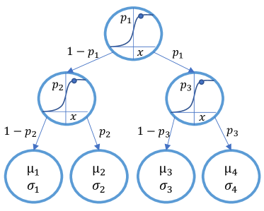
(a) Soft tree

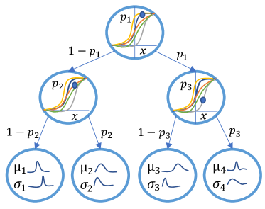
(b) Bayesian soft tree

Figure 1: Standard vs. Bayesian soft decision tree. In a standard soft tree each weight is assigned a fixed value, while in a Bayesian soft tree each weight is a distribution.

Likelihood

We define the likelihood of the soft tree as

$$p\mathopen{}\left(y\,|\,x,\theta\right)\mathclose{}=\sum_{l\in L}P\mathopen{}\left(l\,|\,x,\phi\right)\mathclose{}p\mathopen{}\left(y\,|\,x,l,\psi\right)\mathclose{},$$ (6)

where $L$ is the set of tree leaves (terminal nodes) and $\theta=\left\{\phi,\psi\right\}$ are the parameters of the soft tree.

$P\mathopen{}\left(l\,|\,x,\phi\right)\mathclose{}$, the first term inside the sum in Equation 6, is the probability that the input $x$ is routed to the leaf $l$, defined as:

$$P\mathopen{}\left(l\,|\,x,\phi\right)\mathclose{}=\prod_{n\in\text{Path}\mathopen{}\left(l\right)\mathclose{}}\Bigl{[}P\mathopen{}\left(r\,|\,n,x,\phi\right)\mathclose{}^{n{\searrow}l}\\[-15.00002pt] P\mathopen{}\left(\neg r\,|\,n,x,\phi\right)\mathclose{}^{l{\swarrow}n}\Bigr{]},$$ (7)

where $\text{Path}\mathopen{}\left(l\right)\mathclose{}$ the set of tree nodes on the path from the root to the leaf $l$, $n{\searrow}l=1$ if the leaf $l$ is in the right subtree of node $n$, $l{\swarrow}n=1$ if it is in the left subtree, and $P\mathopen{}\left(r\,|\,n,x,\phi\right)\mathclose{}$ is the probability that $x$ is routed to the right subtree at the node $n$, with $P\mathopen{}\left(\neg r\,|\,n,x,\phi\right)\mathclose{}=1-P\mathopen{}\left(r\,|\,n,x,\phi\right)\mathclose{}$. We parametrize $P\mathopen{}\left(r\,|\,n,x,\phi\right)\mathclose{}$ using a soft gating function $f_{\phi}$:

$$P\mathopen{}\left(r\,|\,n,x,\phi\right)\mathclose{}=f_{\phi}\mathopen{}\left(x,n\right)\mathclose{},$$ (8)

restricting $f_{\phi}\mathopen{}\left(x,n\right)\mathclose{}\in\mathopen{}\left[0,1\right]\mathclose{}$ for all $x$ and $n$. In this work, we choose a simple linear gating function (Feng et al.,, 2020; Frosst and Hinton,, 2017; Irsoy et al.,, 2012; Luo et al.,, 2021):

$$f_{\phi}\mathopen{}\left(x,n\right)\mathclose{}=\sigma\mathopen{}\left(\beta\mathopen{}\left(w_{n}^{T}x+b_{n}\right)\mathclose{}\right)\mathclose{},$$ (9)

where $\sigma$ is the standard sigmoid function, $\beta$ is an inverse temperature parameter used to regularize the function during training (Frosst and Hinton,, 2017), and $\phi=\left\{\mathopen{}\left(w_{n},b_{n}\right)\mathclose{}\right\}_{n\in N}$ are the parameters of the function for the set of tree nodes $N$.

The second term inside the sum in Equation 6, $p\mathopen{}\left(y\,|\,x,l,\psi\right)\mathclose{}$, is the predictive probability when the input $x$ is routed to the leaf $l$. In this work, we consider two variations of this term: a constant leaf model, and a linear leaf model. In the constant leaf model, the output at each leaf is independent of the input:

$$p\mathopen{}\left(y\,|\,x,l,\psi\right)\mathclose{} =p\mathopen{}\left(y\,|\,l,\psi\right)\mathclose{}$$ (10)

$$=\mathcal{N}\mathopen{}\left(y\,|\,\mu_{l},\operatorname{softplus}\mathopen{}\left(\alpha_{l}\right)\mathclose{}^{2}\right)\mathclose{},$$ (11)

where $\psi=\left\{(\mu_{l},\alpha_{l})\right\}_{l\in L}$. In the linear leaf model, on the other hand, the parameters of the Gaussian are linear in the input:

$$p\mathopen{}\left(y\,|\,x,l,\psi\right)\mathclose{} =\mathcal{N}\mathopen{}\left(y\,|\,\mu_{l}\mathopen{}\left(x\right)\mathclose{},\sigma_{l}^{2}\mathopen{}\left(x\right)\mathclose{}\right)\mathclose{}$$ (12)

$$\mu_{l}\mathopen{}\left(x\right)\mathclose{} =w_{l}^{T}x+b_{l}$$ (13)

$$\sigma_{l}\mathopen{}\left(x\right)\mathclose{} =\operatorname{softplus}\mathopen{}\left(\hat{w}_{l}^{T}x+\hat{b}_{l}\right)\mathclose{}$$ (14)

where $\psi=\left\{(w_{l},b_{l},\hat{w}_{l},\hat{b}_{l})\right\}_{l\in L}$ and $\operatorname{softplus}\mathopen{}\left(x\right)\mathclose{}=\text{log}(1+\text{exp}(x))$. We use $\operatorname{softplus}$ functions to constrain the standard deviation parameters to remain strictly positive, while ensuring numerical stability (Blundell et al.,, 2015).

Prior

We use a spherical, zero centered Gaussian prior for the model parameters:

$$p\mathopen{}\left(\theta\right)\mathclose{}=\mathcal{N}\mathopen{}\left(\theta\,|\,0,\tau^{2}\mathbb{I}\right)\mathclose{}.$$ (15)

Note that for a constant leaf model we put this prior on the inverse softplus of the standard deviation at each leaf, which restricts the variance to stay strictly positive.

Variational posterior

We use the variational distribution proposed by Tomczak et al., (2020), which is a Normal distribution with a low-rank covariance matrix:

$$q(\theta)=\mathcal{N}\mathopen{}\left(\theta\,|\,\mu,\text{diag}[\sigma^{2}]+VV^{T}\right)\mathclose{}$$ (16)

where $\sigma\in\mathbb{R}^{p}$ and $V$ is a matrix of rank $k$. The hyperparameter $k$ determines the rank of the covariance matrix, and hence the expressivity of the posterior. If $\theta\in{}^{p}$, choosing $k=p$ allows learning arbitrary covariance matrices, but increases the memory requirements and computational cost. As a result, in our experiments we typically choose $k<p$. This choice of the variational posterior and the prior admits an analytical KL-divergence which is detailed in Section 1.1 in the supplementary material.

Input: Prior parameters $a_{\sigma}$ and $b_{\sigma}$

          $T$ the number of soft trees in the GBM

Data: $\left\{X,y\right\}$

Fit variational soft tree $f_{\theta_{1}}$ to $\left\{X,y\right\}$

for $t\in[2,\dots T]$ do

       Sample parameters for all models $f_{\theta_{j}}:\theta_{j}\sim q_{j}$ for $j=1\dots t-1$

       Compute the residual vector: $r_{t}=y-\sum_{j=1}^{t-1}f_{\theta_{j}}\mathopen{}\left(X\right)\mathclose{}$

       Fit the new model $f_{\theta_{t}}$ to $\left\{X,r_{t}\right\}$

end for

Sample parameters $\theta=\left\{\theta_{j}\right\}_{j=1}^{T}$ where $\theta_{j}\sim q_{j}$

Compute final residuals $r=y-F_{\theta}\mathopen{}\left(X\right)\mathclose{}$

Sample $\sigma^{2}\sim\text{inverse-Gamma}(a_{\sigma}+n,b_{\sigma}+r^{T}r)$

Algorithm 1 Gradient boosted variational soft trees

4.2 Gradient boosted variational soft trees

In order to increase the expressivity of the variational soft tree, we propose to use these models as weak learners in a gradient boosting machine that we refer to as a variational soft GBM (VSGBM). More formally, the model is defined as

$$F_{\theta}\mathopen{}\left(x\right)\mathclose{}=\sum_{t=1}^{T}f_{\theta_{t}}\mathopen{}\left(x\right)\mathclose{}+\epsilon\quad\text{where}\quad\epsilon\sim\mathcal{N}\mathopen{}\left(\epsilon\,|\,0,\sigma^{2}\right)\mathclose{}$$ (17)

where $f_{\theta_{t}}$ is a variational soft tree with parameters $\theta_{t}$, $T$ is the number of trees in the ensemble and $\sigma$ is a scale parameter. We consider variational soft trees $f_{\theta_{t}}$ that output the estimated mean value of the target and no standard deviation. Hence the variational soft GBM has a homoskedastic (input-independent) variance model. Heteroskedastic (input-dependent) uncertainty could in principle be modeled by returning the predictive variances from the weak learners alongside the predictive means, and combining them upstream. In our early experiments this configuration proved to be costly to train (it doubles the number of model parameters), and made the training unstable (the gradient boosting loss had high variance). In prior work Pratola et al., (2017) train a separate ensemble to capture aleatoric uncertainty, likely to avoid this instability.

Inspired by He and Hahn, (2020), we place an $\text{inverse-Gamma}(a_{\sigma},b_{\sigma})$ prior on $\sigma^{2}$, yielding an $\text{inverse-Gamma}(a_{\sigma}+n,b_{\sigma}+r^{T}r)$ posterior, where $n$ is the number of data samples and $r=y-F_{\theta}\mathopen{}\left(X\right)\mathclose{}$ is the residual vector. The variational soft GBM is fit following the procedure described in Algorithm 1. Once trained, samples from the approximate posterior of the variational soft GBM are obtained by drawing parameters from the variational distribution of each variational soft tree model in the ensemble. The predictive distribution is then approximated by Monte Carlo integration of the likelihood as per Equation 2, i.e. by aggregating the predictions of the variational soft trees as defined by Equation 17 for different posterior samples.

5 EXPERIMENTS

In this section we evaluate the variational soft tree and variational soft GBM on regression, out-of-distribution detection and multi-armed bandits. Although we are not measuring model calibration directly, like prior work we assume that model calibration and performance on these tasks are correlated. When reporting results, we bold the highest score, as well as any score if its error bar and the highest score’s error bar overlap, considering the difference to not be statistically significant.

5.1 Regression

Table 1: Test log-likelihood of evaluated methods on regression datasets. We find that variational soft decision trees (VST) and variational soft GBMs (VSGBM) perform strongly compared to baselines in terms of test log-likelihood, both methods out-performing them on 7/10 datasets.

Model	Power	Protein	Boston	Naval	Yacht	Song	Concrete	Energy	Kin8nm	Wine
Deep ensemble	-1.404 $\pm$ 0.001	-1.422 $\pm$ 0.000	-1.259 $\pm$ 0.007	-1.412 $\pm$ 0.000	-1.112 $\pm$ 0.009	-1.415 $\pm$ 0.001	-1.390 $\pm$ 0.001	-1.677 $\pm$ 0.073	-1.416 $\pm$ 0.000	-1.725 $\pm$ 0.075
XBART (1 tree)	-0.096 $\pm$ 0.003	-1.136 $\pm$ 0.003	-0.508 $\pm$ 0.042	-0.485 $\pm$ 0.419	-1.110 $\pm$ 0.021	-1.151 $\pm$ 0.006	-0.793 $\pm$ 0.079	-0.848 $\pm$ 0.567	-1.153 $\pm$ 0.014	-1.250 $\pm$ 0.008
SGLB (1 tree)	-1.425 $\pm$ 0.027	-1.499 $\pm$ 0.002	-1.361 $\pm$ 0.044	-1.410 $\pm$ 0.009	-0.891 $\pm$ 0.047	-1.305 $\pm$ 0.007	-1.748 $\pm$ 0.050	-1.078 $\pm$ 0.006	-1.659 $\pm$ 0.015	-1.559 $\pm$ 0.033
VST (const.)	-0.032 $\pm$ 0.010	-0.719 $\pm$ 0.005	-0.920 $\pm$ 0.002	-0.555 $\pm$ 0.088	-0.193 $\pm$ 0.024	-0.733 $\pm$ 0.010	-0.999 $\pm$ 0.006	-0.710 $\pm$ 0.280	-0.877 $\pm$ 0.014	-1.458 $\pm$ 0.615
VST (linear)	-0.024 $\pm$ 0.002	-0.631 $\pm$ 0.011	-0.682 $\pm$ 0.004	-0.335 $\pm$ 0.026	-0.754 $\pm$ 0.005	-0.579 $\pm$ 0.002	-0.461 $\pm$ 0.070	-0.377 $\pm$ 0.123	-0.707 $\pm$ 0.012	-3.067 $\pm$ 1.168
XBART	-0.001 $\pm$ 0.006	-1.136 $\pm$ 0.003	-0.462 $\pm$ 0.054	-0.008 $\pm$ 0.130	-1.116 $\pm$ 0.023	-1.018 $\pm$ 0.002	-0.581 $\pm$ 0.024	-0.462 $\pm$ 0.054	-1.057 $\pm$ 0.007	-1.251 $\pm$ 0.010
SGLB	-0.500 $\pm$ 0.001	-1.204 $\pm$ 0.002	-0.504 $\pm$ 0.013	-0.877 $\pm$ 0.004	-0.018 $\pm$ 0.009	-0.907 $\pm$ 0.001	-0.931 $\pm$ 0.010	-0.232 $\pm$ 0.009	-1.125 $\pm$ 0.002	-1.220 $\pm$ 0.006
VSGBM (const.)	-0.002 $\pm$ 0.011	-1.039 $\pm$ 0.005	-0.567 $\pm$ 0.062	-0.573 $\pm$ 0.311	-0.045 $\pm$ 0.912	-0.933 $\pm$ 0.008	-0.465 $\pm$ 0.040	-0.227 $\pm$ 0.038	-0.457 $\pm$ 0.021	-1.192 $\pm$ 0.007
VSGBM (linear)	-0.015 $\pm$ 0.011	-1.051 $\pm$ 0.012	-0.462 $\pm$ 0.054	-0.542 $\pm$ 0.295	-0.033 $\pm$ 0.049	-0.729 $\pm$ 0.019	-0.591 $\pm$ 0.079	-0.057 $\pm$ 0.134	-0.363 $\pm$ 0.031	-1.167 $\pm$ 0.004

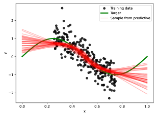
(a) Variational soft tree

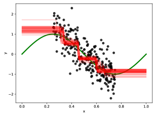
(b) XBART

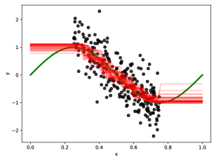
(c) SGLB

Figure 2: Variational soft trees (VST) show high uncertainty in the tails outside of the data support while closely agreeing with the mean inside the support. Sampled function show more diversity in tails with VSTs than with XBART and SGLB. The VST uses linear leaves, while XBART and SGLB use constant leaves.

We consider a suite of regression datasets used by Malinin et al., (2020) described in Table 4 in supplementary material. We perform 10-fold cross validation on the training data and report the mean and standard deviation of the test log-likelihood and root mean square error (RMSE) of our models across the folds. We compare our variational soft decision trees (VST) and variational soft GBM (VSGBM) with two Bayesian GBMs (XBART (He and Hahn,, 2020) and SGLB (Ustimenko and Prokhorenkova,, 2020)), an ensemble of neural networks, and XGBoost (Chen and Guestrin,, 2016). When comparing models to VSTs, we consider baselines with an ensemble size of one, and otherwise multiple ensemble members when comparing with the VSGBM. The only exception is the ensemble of deep neural networks for which we always use an ensemble of ten models to measure epistemic uncertainty.

Variational soft decision tree

We find that our model performs well in terms of test log-likelihood and RMSE across the considered datasets (see Tables 1 and 6), which confirms that soft decision trees are well-suited to tabular data (Luo et al.,, 2021). VSTs outperform the baselines on 7/10 datasets in terms of log-likelihood, and 3/10 datasets in terms of RMSE, also matching the log-likehood and RMSE of best performing baselines on 1/10 and 3/10 datasets respectively. In addition, soft decision trees with linear leaves perform better than equivalent constant leaf models on 8/10 datasets in terms of log-likelihood and 5/10 in terms of RMSE, bringing evidence that linear leaf models are more expressive than constant leaf models.

VSTs are less competitive when trained on small datasets like boston (506 training examples) and yacht (308 training examples). We hypothesize that in these cases the model underfits the data due to the choice of the prior. The parameters of the prior were chosen by hyper-parameter tuning with the validation ELBO objective, and the underfitting behavior could be an artifact of this tuning procedure. An alternative hypothesis is that a normal prior is simply ill-suited to this model. Choosing priors for complex, deep models is difficult, and is an active research direction in Bayesian deep learning (Flam-Shepherd,, 2017; Fortuin et al.,, 2021; Krishnan et al.,, 2020; Vladimirova et al.,, 2018).

Variational soft GBM

VSGBMs perform competitively in terms of log-likelihood compared to the baselines (see Tables 1 and 6), yielding the best log-likelihood on 7/10 datasets. The VSGBMs perform on par with baselines on power and boston, worse on yacht but better on the other datasets. However, VSGBMs are less competitive in terms of RMSE when compared to XGBoost that yields smaller RMSE on all but three datasets. Compared to other baselines, VSGBM consistently outperforms the deep ensemble, and performs favorably when compared to SGLB and XBART. In addition, we find that VSGBMs with linear leaves perform slightly better than equivalent constant leaf models, outperforming them on 4/10 datasets in terms of log-likelihood and 3/10 in terms of RMSE, while also matching the log-likelihod and RMSE of constant leaves on 5/10 and 6/10 datasets respectively.

Compared to a VST, a VSGBM performs better in terms of RMSE on all datasets but two where both models score equally well. However, VSTs obtain higher log-likelihoods than VSGBMs on 5/10 datasets, equivalent scores on 2/10 and performs worse on 3/10. We explain this by the simpler variance model used in the VSGBM, which does not allow for heteroskedastic (input dependent) uncertainty.

Uncertainty estimation visualization

An important property of a reliable predictive model is its increased predictive uncertainty for inputs in regions with little training data. To understand if VSTs demonstrate this behavior, we plot functions sampled from the variational posterior for simple synthetic datasets, and compare them to functions sampled from XBART and SGLB posteriors. We plot the sampled functions in Figures 2 and 5.

We find that VSTs indeed capture the uncertainty outside of the support of the data better than both XBART and SGLB: functions agree with the true mean within the support of the data, but diverge outside of it.

5.2 OOD detection

Table 2: OOD detection AUROC scores with variational soft trees (VST) and variational soft GBMs (VSGBM) against baselines (higher is better). Variational soft decision trees and variational soft GBMs perform well on out of distribution detection, yielding the best score on 6/10 and 5/10 datasets respectively.

Model	Power	Protein	Boston	Naval	Yacht	Song	Concrete	Energy	Kin8nm	Wine
Deep ensemble	0.540 $\pm$ 0.015	0.504 $\pm$ 0.003	0.545 $\pm$ 0.023	1.000 $\pm$ 0.000	0.691 $\pm$ 0.088	0.510 $\pm$ 0.007	0.767 $\pm$ 0.042	0.554 $\pm$ 0.036	0.508 $\pm$ 0.005	0.547 $\pm$ 0.019
XBART (1 tree)	0.562 $\pm$ 0.018	0.684 $\pm$ 0.015	0.656 $\pm$ 0.042	0.578 $\pm$ 0.050	0.603 $\pm$ 0.021	0.608 $\pm$ 0.033	0.671 $\pm$ 0.028	0.852 $\pm$ 0.141	0.525 $\pm$ 0.010	0.548 $\pm$ 0.016
SGLB (1 tree)	0.593 $\pm$ 0.025	0.760 $\pm$ 0.018	0.732 $\pm$ 0.039	0.770 $\pm$ 0.021	0.607 $\pm$ 0.035	0.589 $\pm$ 0.035	0.723 $\pm$ 0.018	0.969 $\pm$ 0.003	0.519 $\pm$ 0.005	0.571 $\pm$ 0.021
VST (const.)	0.591 $\pm$ 0.025	0.866 $\pm$ 0.018	0.712 $\pm$ 0.020	0.884 $\pm$ 0.024	0.718 $\pm$ 0.048	0.560 $\pm$ 0.025	0.677 $\pm$ 0.049	0.863 $\pm$ 0.045	0.529 $\pm$ 0.016	0.796 $\pm$ 0.010
VST (linear)	0.618 $\pm$ 0.024	0.920 $\pm$ 0.019	0.698 $\pm$ 0.020	1.000 $\pm$ 0.000	0.655 $\pm$ 0.015	0.601 $\pm$ 0.015	0.840 $\pm$ 0.013	0.996 $\pm$ 0.003	0.586 $\pm$ 0.011	0.742 $\pm$ 0.036
XBART	0.572 $\pm$ 0.011	0.678 $\pm$ 0.016	0.741 $\pm$ 0.041	0.912 $\pm$ 0.033	0.607 $\pm$ 0.026	0.565 $\pm$ 0.013	0.818 $\pm$ 0.020	0.837 $\pm$ 0.146	0.541 $\pm$ 0.011	0.549 $\pm$ 0.021
SGLB	0.600 $\pm$ 0.011	0.874 $\pm$ 0.006	0.738 $\pm$ 0.027	0.907 $\pm$ 0.011	0.662 $\pm$ 0.036	0.697 $\pm$ 0.029	0.763 $\pm$ 0.024	0.973 $\pm$ 0.007	0.508 $\pm$ 0.004	0.613 $\pm$ 0.019
VSGBM (const.)	0.569 $\pm$ 0.018	0.890 $\pm$ 0.011	0.775 $\pm$ 0.101	1.000 $\pm$ 0.000	0.663 $\pm$ 0.055	0.586 $\pm$ 0.014	0.666 $\pm$ 0.033	0.901 $\pm$ 0.018	0.562 $\pm$ 0.015	0.625 $\pm$ 0.019
VSGBM (linear)	0.571 $\pm$ 0.010	0.950 $\pm$ 0.016	0.795 $\pm$ 0.025	1.000 $\pm$ 0.000	0.618 $\pm$ 0.020	0.602 $\pm$ 0.006	0.763 $\pm$ 0.023	0.993 $\pm$ 0.008	0.608 $\pm$ 0.012	0.688 $\pm$ 0.027

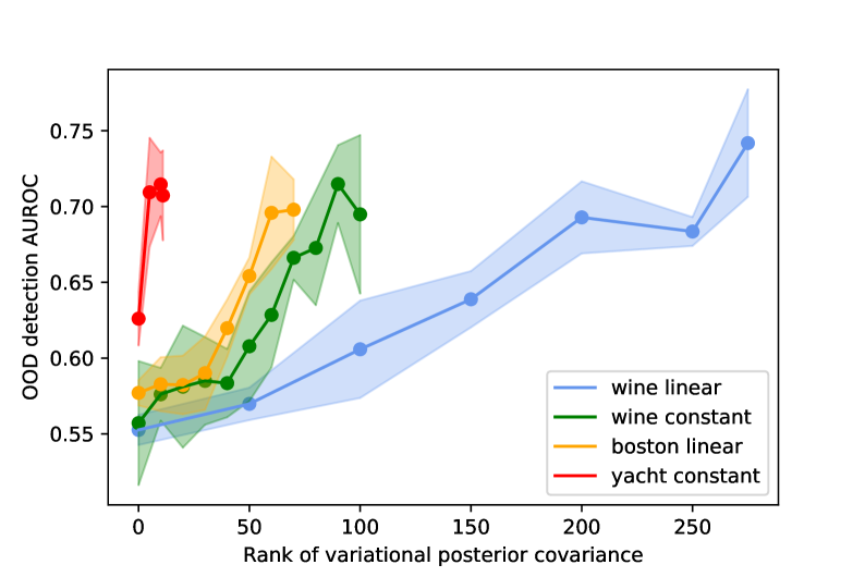
Figure 3: OOD detection AUROC score vs. the rank of the variational posterior covariance matrix in variational soft trees (VST). The quality of the OOD detection generally increases with the rank of the approximate posterior covariance. As we consider a large number of different model and dataset configurations, we only present the ones for which the increase in AUROC is most significant. The rightmost point of each plot corresponds to a full rank covariance approximation.

Out-of-distribution (OOD) data is data that is sampled from a distribution that is sufficiently different from the training data distribution. It has been observed in prior work (Ma and Hernández-Lobato,, 2021; Tomczak et al.,, 2020) that an effective Bayesian model will show high epistemic uncertainty when presented with OOD data, so we further evaluate our models by testing if their epistemic uncertainty is predictive of OOD data.

Following the setup of Malinin et al., (2020), we define OOD data by selecting a subset of data from a different dataset. To perform OOD detection, we compute the epistemic uncertainty of each sample under our models and evaluate how well a single splitting threshold separates the epistemic uncertainty of in-distribution and OOD samples, as proposed by Mukhoti et al., (2021). Epistemic uncertainty is measured as the variance of the mean prediction with respect to samples from the posterior or the ensemble. The detection performance is quantified using the area under the receiver operating characteristic curve (AUROC). We report the mean and standard deviation of the AUROC of each model across 10 folds of cross-validation. As before, we compare our VSTs and VSGBMs with XBART, SGLB and a deep ensemble.

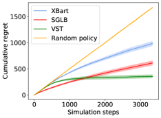
(a) Financial

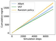
(b) Mushroom

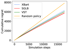
(c) Jester

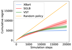
(d) Exploration

Figure 4: Bandit results. We find that the variational soft tree (VST) converges to near zero instantaneous regret on the financial bandit and performs competitively compared to baselines in the bandit setting.

We find that variational soft decision trees perform well on OOD detection, outperforming baselines on 6/10 datasets and tying on others (see Table 2). VSGBMs also perform well, yielding the best scores on 5/10 datasets and additionally matching best baselines on 2/10 (see Table 2). However, the improvements over the top baselines are less significant than with variational soft decision trees. As expected, we find that increasing the rank of the approximate variational posterior increases the OOD performance, although the significance of the improvement depends on the dataset (see Figure 3). This effect is most prominent with variational soft decision trees, and is less so in VSGBMs.

5.3 Bandits

Table 3: Cumulative regret of the bandits using variational soft trees (VST) vs. baselines. We find that VST performs competitively compared to baselines, achieving the lowest cumulative regret on 2/4 bandits.

Bandit	financial	exploration	mushroom	jester
Random policy	1682.05 $\pm$ 20.23	18904.95 $\pm$ 24.3700	1791.28 $\pm$ 29.61	7845.28 $\pm$ 26.99
VST	0357.47 $\pm$ 34.32	07054.60 $\pm$ 748.790	1412.55 $\pm$ 5.640	6048.99 $\pm$ 42.26
SGLB	0613.12 $\pm$ 45.96	09469.07 $\pm$ 1197.60	doesn’t work	5762.89 $\pm$ 82.10
XBART	0984.86 $\pm$ 47.59	5039.93 $\pm$ 322.63	1577.70 $\pm$ 61.56	6305.43 $\pm$ 31.97

We further evaluate the VST by using it in Thompson sampling (Thompson,, 1933) on four different multi-armed bandit problems (see Section 2.3 in the supplementary material for more detail on the datasets), comparing to XBART and SGLB as before. We do not experiment with VSGBMs in the bandit setting due to computational cost. In this setting, the model has to be re-trained after every update, and training a VSGBM is expensive: boosting is sequential by nature, and VST weak learners require a number of gradient descent iterations to converge. Each bandit simulation is run five times with different random seeds, and we report the mean and the standard deviation of the cumulative regret across the simulations.

The predictive uncertainty of VST is competitive in this setting as well, as shown in Table 3. The VST obtains the lowest cumulative regret on the mushroom and financial datasets, converging to near zero instantaneous regret on the latter (see Figure 4). On the jester dataset, the VST demonstrates second best cumulative regret, although the performance of all three models is comparable to the random policy. We explain this by the difficulty of the regression problem in this particular dataset. Finally, just like on jester, the VST shows second best cumulative regret on the exploration dataset.

6 DISCUSSION

In this work we proposed to perform variational inference to approximate the Bayesian posterior of a soft decision tree. We use a variational distribution that allows trading off memory and computation for a richer posterior approximation. Using soft decision trees models as weak learners, we build a variational soft GBM that is more expressive than the individual trees, but preserves their well-calibrated predictive uncertainty. We find that both variational soft trees and variational soft GBMs perform well on tabular data compared to strong baselines, and provide useful uncertainty estimates for OOD detection and multi-armed bandits.

An important direction for future work is to speed up the training of variational soft trees and GBMs. This is especially important when working in the low-data regime (${<}10^{4}$ samples), where our models are slower than the baseline based on standard decision trees, and in the context of multi-armed bandits, where the model needs to be updated repeatedly. For the latter, an alternative direction is to adapt our models for continual learning by implementing an efficient Bayesian update, which would accelerate sequential learning tasks like multi-armed bandits, Bayesian optimization and active learning. Finally, addapting VST and VSGBM to the classification setting is an interesting direction for future work. Classification with tabular data is important in many applications, many of which might also benefit from well-calibrated predictive uncertainties (Ebbehoj et al.,, 2021; Mustafa and Rahimi Azghadi,, 2021).

1 Additional method details

1.1 Variational inference

We use the variational distribution proposed by Tomczak et al., (2020), which is a normal distribution with a low-rank covariance matrix:

$$q(\theta)=\mathcal{N}\mathopen{}\left(\theta\,|\,\mu,\text{diag}[\sigma^{2}]+VV^{T}\right)\mathclose{}$$ (18)

where $\mu\in\mathbb{R}^{p}$ is the mean of the normal distribution over parameters, $\text{diag}[\sigma^{2}]\in\mathbb{R}^{p\times p}$ is the diagonal component of the covariance with $\sigma\in\mathbb{R}^{p}$, and $V\in\mathbb{R}^{p\times k}$ is the rank $k$ component of the covariance. The hyperparameter $k$ determines the rank of the covariance matrix, and hence the expressivity of the posterior. Choosing $k=p$ allows learning arbitrary covariance matrices, but increases the memory requirements and computational cost. As a result, in our experiments we typically choose $k<p$. We fit the variational soft tree by maximizing the evidence lower bound (ELBO):

$$\text{ELBO}={\mathop{{}\mathbb{E}}}_{\theta\sim q\mathopen{}\left(\theta\right)\mathclose{}}\mathopen{}\left[\log p\mathopen{}\left(y\,|\,x,\theta\right)\mathclose{}\right]\mathclose{}-D_{\mathrm{KL}}\mathopen{}\left(q\mathopen{}\left(\theta\right)\mathclose{}\,\|\,p\mathopen{}\left(\theta\right)\mathclose{}\right)\mathclose{}.$$ (19)

We compute a Monte Carlo estimate of the expectation:

$${\mathop{{}\mathbb{E}}}_{\theta\sim q}\mathopen{}\left[\log p\mathopen{}\left(y\,|\,x,\theta\right)\mathclose{}\right]\mathclose{}\approx\frac{1}{m}\sum_{i=1}^{m}\log p\mathopen{}\left(y\,|\,x,\theta^{(i)}\right)\mathclose{},$$ (20)

where $\theta^{(i)}\sim q\mathopen{}\left(\theta\right)\mathclose{}$. For the chosen posterior in Equation 18 and an isotropic Gaussian prior $p\mathopen{}\left(\theta\right)\mathclose{}=\mathcal{N}\mathopen{}\left(\theta\,|\,0,\gamma\mathbb{I}\right)\mathclose{}$, the KL divergence term is available in a closed form:

$$D_{\mathrm{KL}}\mathopen{}\left(q\mathopen{}\left(\theta\right)\mathclose{}\,\|\,p\mathopen{}\left(\theta\right)\mathclose{}\right)\mathclose{}=\frac{1}{2}\left[\sum_{d=1}^{p}\left(\frac{\sigma_{d}^{2}}{\gamma}-\log\>\sigma_{d}^{2}\right)+\frac{1}{\gamma}\sum_{i=1}^{k}||v_{i}||_{2}^{2}-\Delta+\frac{1}{\gamma}||\mu||_{2}^{2}+p(\log\>\gamma-1)\right],$$ (21)

where $V=[v_{1},\dots v_{k}]\in\mathbb{R}^{p\times k}$, $\sigma\in\mathbb{R}^{p}$ and $\Delta=\log\det(\mathbb{I}_{k}+V^{T}\text{diag}[{\sigma^{2}}]^{-1}V)$.

2 Experimental details

2.1 Regression

We consider a suite of regression datasets from Malinin et al., (2020) to measure the expressivity of our model. Table 4 summarizes the number of examples and features in each dataset. We preprocess the datasets by encoding categorical variables as one-hot vectors and normalizing each feature to have zero mean and unit variance. We further split the datasets into train (80%) and test (20%) data, and perform 10-fold cross validation on the training data. We report the mean and the standard deviation of the test log-likelihood and root mean square error (RMSE) across all folds.

Table 4: Regression dataset description

Dataset	Boston	Naval	Power	Protein	Yacht	Song	Concrete	Energy	Kin8nm	Wine
Number samples	506	11 934	9 568	45 730	308	514 345	1 030	768	8 192	1 599
Number features	13	16	4	9	6	90	8	8	8	11

2.2 OOD detection

Following the setup from Malinin et al., (2020), we consider the test data to be the in-distribution (ID) data, and create a dataset of OOD data by taking a subset of the song dataset of the same size. We select a subset of features from the song dataset in order to match the feature dimension of the ID dataset. The only exception is the song dataset itself, for which we use the Relative location of CT slices on axial axis dataset from Graf et al., (2011) as OOD data. In both settings, categorical features are encoded as one-hot vectors, and all features are normalized to have zero mean and unit variance. We use a one-node decision tree to find the splitting threshold for the epistemic uncertainty that would separate ID and ODD data.

2.3 Bandit

We consider the following datasets for our bandit experiments:

Financial

The financial bandit (Riquelme et al.,, 2018) was created by pulling the stock prices of $d=21$ publicly traded companies in NYSE and Nasdaq, for the last 14 years for a total of $n=3713$ samples. For each day, the context was the price difference between the beginning and end of the session for each stock. The arms are synthetically created to be a linear combination of the contexts, representing $k=8$ different portfolios.

Jester

This bandit problem is taken from Riquelme et al., (2018). The Jester dataset (Goldberg et al.,, 2001) provides continuous ratings in $[-10,10]$ for 100 jokes from 73 421 users. The authors find a complete subset of $n=19\,181$ users rating all 40 jokes. We take $d=32$ of the ratings as the context of the user, and $k=8$ as the arms. The agent recommends one joke, and obtains the reward corresponding to the rating of the user for the selected joke.

Exploration

The exploration bandit tests the extent to which the models explore the different arms. The reward function of each arm is sparse and requires maintaining high uncertainty to discover the context values for which the reward is high. The reward given input $x$ and selected arm $a$ is given by:

$$r(x,a)=\sigma(\beta(x+\alpha-\text{offset}[a]))-\sigma(\beta(x-\alpha-\text{offset}[a]))+\epsilon$$ (22)

where $\sigma(x)=1\mathbin{/}(1+e^{-x})$ is the sigmoid function, $\alpha,\beta\in\mathbb{R}$ are constants, $\epsilon\sim N(0,\delta^{2})$, and $\text{offset}[a]$ is a function mapping each arm $a$ to a particular offset. Intuitively, this reward is composed of a smooth unit valued “bump” per arm and is otherwise 0. The positions of the “bumps” across arms are disjoint and barely overlap. Furthermore, the context is sampled uniformly at random in the interval $[-1,1]$. We run this bandit for 20 000 steps.

Mushroom

This bandit problem is taken from Riquelme et al., (2018). The Mushroom Dataset (Dua and Graff,, 2017) contains $n=7\,310$ samples, 22 attributes per mushroom, and two classes: poisonous and safe. The agent must decide whether to eat a given mushroom or not. Eating a safe mushroom provides reward of 5. Eating a poisonous mushroom delivers reward 5 with probability 1/2 and reward -35 otherwise. If the agent does not eat a mushroom, then the reward is 0.

2.4 Implementation

We implement the variational soft decision tree and variational soft GBM using the Jax (Bradbury et al.,, 2018) and DM-Haiku (Hennigan et al.,, 2020) Python libraries. We fit our models using the Adam (Kingma and Ba,, 2014) optimizer. Hyperparameter optimization was conducted using Amazon SageMaker’s automatic model tuning that uses Bayesian optimisation to explore the hyperparameter space. We define the set of hyperparameters that the Bayesian optimisation needs to explore, as well as the optimization objective. The service then runs a series of model tuning jobs with different hyperparameters to find the set of values which minimize the objective. We use the same hyperparameter ranges as (He and Hahn,, 2020) and (Ustimenko and Prokhorenkova,, 2020), summarized in Table 5.

Table 5: Hyperparameter tuning ranges.

VSGBM		XBART		XGBOOST		Deep ensemble		VST		SGLB
Learning rate	$[0.0001,0.001]$	s	$[1,300]$	Learning rate	$[0.001,0.1]$	Learning rate	$[0.0001,0.001]$	Learning rate	$[0.0001,0.001]$	Learning rate	$\left\{0.001,0.01,0.1\right\}$
Prior scale	$[0.01,2.5]$	Tau	$[1,300]$	Tree depth	$\left\{1,\dots,6\right\}$	Num. layers	$\left\{2,\dots,5\right\}$	Prior scale	$[0.01,2.5]$	Tree depth	$\left\{3,\dots,6\right\}$
Max. depth	$\left\{1,\dots,5\right\}$	Beta	$[0.75,2]$	Lambda	$[0.001,1]$	Hidden dim.	$\left\{10,\dots,50\right\}$	Max. depth	$\left\{1,\dots,5\right\}$	Num. learners	$\left\{1,\dots,1000\right\}$
Beta	$[1,50]$	Num. learners	$[1,100]$	Alpha	$[0.001,1]$	Dropout rate	$[0.1,0.4]$	Beta	$[1,50]$
Num. learners	$\left\{1,\dots,10\right\}$	Burn-in	$\left\{15\right\}$	Num. learners	$\left\{1,\dots,1000\right\}$	Prior scale	$[0.001,2.5]$
Prior sigma alpha	$[2.5,5]$	Alpha	$\left\{0.95\right\}$
Prior sigma beta	$[0.1,5]$	Kappa	$\left\{3\right\}$

3 Additional experimental results

3.1 Regression

In this section we present additional regression results reporting the root mean square error (RMSE) of evaluated methods across the considered baselines, see Table 6. We find that the VST performs well in terms of test RMSE across datasets: our model outperforms the baselines on 3/10 datasets and matching the RMSE of the top baselines on 3/10. This further confirms that soft decision trees perform well on tabular data (Luo et al.,, 2021).

We observe that VSGBMs are generally weaker in terms of RMSE compared to XGBoost. XGBoost yields a smaller RMSE on all but three datasets, where VSGBM performs better on one and ties on two. This result is not surprising as XGBoost is the gold standard for fitting tabular data. Compared to other baselines, VSGBM systematically outperforms deep ensembles, and performs favorably compared to SGLB and XBART. Compared to a single variational soft tree, VSGBMs perform better in terms of RMSE on all datasets but two where they ties.

Table 6: Test RMSE of evaluated methods on regression datasets. We find that variational soft decision trees (VST) compares well with baselines in terms of test RMSE, out-performing them on 3/10 datasets and matching the RMSE of the best baselines on three. Variational soft GBM (VSGBM) performs competitively in terms of RMSE compared to SGLB, deep ensemble and XBART, but is generally weaker than XGBoost. This is unsurprising as XGBoost is the state-of-the-art for fitting tabular data.

Model	Power	Protein	Boston	Naval	Yacht	Song	Concrete	Energy	Kin8nm	Wine
Deep ensemble	0.986 $\pm$ 0.001	1.003 $\pm$ 0.001	0.870 $\pm$ 0.004	0.993 $\pm$ 0.001	0.685 $\pm$ 0.002	0.999 $\pm$ 0.001	0.972 $\pm$ 0.001	1.007 $\pm$ 0.009	0.998 $\pm$ 0.001	1.013 $\pm$ 0.011
XBART (1 tree)	0.243 $\pm$ 0.001	0.693 $\pm$ 0.003	0.356 $\pm$ 0.026	0.339 $\pm$ 0.125	0.052 $\pm$ 0.003	0.680 $\pm$ 0.007	0.474 $\pm$ 0.046	0.406 $\pm$ 0.267	0.703 $\pm$ 0.013	0.815 $\pm$ 0.006
SGLB (1 tree)	0.280 $\pm$ 0.006	0.869 $\pm$ 0.002	0.483 $\pm$ 0.025	0.830 $\pm$ 0.007	0.405 $\pm$ 0.007	0.958 $\pm$ 0.007	0.541 $\pm$ 0.010	0.193 $\pm$ 0.003	0.740 $\pm$ 0.002	0.827 $\pm$ 0.004
XGBoost (1 tree)	0.242 $\pm$ 0.003	0.828 $\pm$ 0.001	0.397 $\pm$ 0.077	0.703 $\pm$ 0.001	0.056 $\pm$ 0.006	0.795 $\pm$ 0.003	0.454 $\pm$ 0.021	0.059 $\pm$ 0.005	0.776 $\pm$ 0.010	0.854 $\pm$ 0.020
VST (const.)	0.239 $\pm$ 0.001	0.827 $\pm$ 0.008	0.538 $\pm$ 0.004	0.359 $\pm$ 0.033	0.477 $\pm$ 0.027	0.710 $\pm$ 0.010	0.592 $\pm$ 0.005	0.483 $\pm$ 0.099	0.550 $\pm$ 0.010	0.788 $\pm$ 0.009
VST (linear)	0.242 $\pm$ 0.001	0.798 $\pm$ 0.011	0.469 $\pm$ 0.003	0.376 $\pm$ 0.002	0.500 $\pm$ 0.004	0.633 $\pm$ 0.006	0.423 $\pm$ 0.066	0.281 $\pm$ 0.044	0.530 $\pm$ 0.018	0.781 $\pm$ 0.008
XBART	0.233 $\pm$ 0.001	0.692 $\pm$ 0.003	0.303 $\pm$ 0.022	0.152 $\pm$ 0.045	0.051 $\pm$ 0.003	0.576 $\pm$ 0.003	0.355 $\pm$ 0.012	0.292 $\pm$ 0.295	0.590 $\pm$ 0.007	0.815 $\pm$ 0.008
SGLB	0.453 $\pm$ 0.001	0.822 $\pm$ 0.001	0.583 $\pm$ 0.004	0.649 $\pm$ 0.002	0.300 $\pm$ 0.004	0.834 $\pm$ 0.001	0.593 $\pm$ 0.002	0.318 $\pm$ 0.002	0.778 $\pm$ 0.001	0.857 $\pm$ 0.002
XGBoost	0.173 $\pm$ 0.003	0.614 $\pm$ 0.004	0.261 $\pm$ 0.012	0.057 $\pm$ 0.001	0.041 $\pm$ 0.006	0.450 $\pm$ 0.001	0.285 $\pm$ 0.014	0.050 $\pm$ 0.001	0.479 $\pm$ 0.019	0.735 $\pm$ 0.014
VSGBM (const.)	0.238 $\pm$ 0.001	0.652 $\pm$ 0.006	0.363 $\pm$ 0.025	0.111 $\pm$ 0.060	0.142 $\pm$ 0.107	0.563 $\pm$ 0.004	0.347 $\pm$ 0.016	0.227 $\pm$ 0.015	0.348 $\pm$ 0.009	0.781 $\pm$ 0.008
VSGBM (linear)	0.242 $\pm$ 0.001	0.663 $\pm$ 0.012	0.297 $\pm$ 0.009	0.074 $\pm$ 0.018	0.134 $\pm$ 0.005	0.483 $\pm$ 0.007	0.341 $\pm$ 0.014	0.183 $\pm$ 0.037	0.316 $\pm$ 0.010	0.769 $\pm$ 0.006

3.2 Uncertainty visualization

In order to demonstrate the quality of the predictive uncertainty of our model, we present additional plots of functions sampled from the VST, comparing these to samples from XBART and SGLB. See Figure 2 and Figure 5. We find that variational soft decision trees model the uncertainty outside of the support of the data better than XBART and SGLB: functions agree with the true mean within the support of the data, but diverge outside of it.

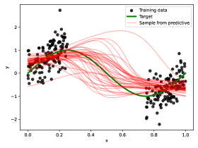
(a) VST

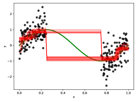
(b) XBART

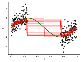
(c) SGLB

Figure 5: In-between uncertainty. Variational soft trees (VST) show high uncertainty between the two blobs of data while closely agreeing with the true mean inside of the data support. The plot for the VST was generated with the linear leaf model.

3.3 Regression visualization

To test the flexiblity of the VST in the regression setting, we fit our model to a step function (Figure 6) and a Daubechies wavelet (Figure 7) as done in (Linero and Yang,, 2017), and plot functions sampled from our model. We see that the VST captures the non-smooth step function as well as the hard decision trees used in XBART and SGLB. On the Daubechies wavelet, however, we find that a VST of a reasonable depth (5) underfits. VSGBM visually improves the fit over a VST, but still underfits the data compared to SGLB and XBART. We hypothesize that this effect is due to the choice of zero mean Gaussian prior on the node weights $w_{n}$ in VSTs and VSGBMs, which encourages smooth functions. This phenomenon is particularly visible when fitting the Daubechies wavelet, a complex function that fluctuates at different frequencies and amplitudes. As expected, increasing the amount of training data reduces underfitting.

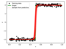
(a) VST (RMSE: 0.2121)

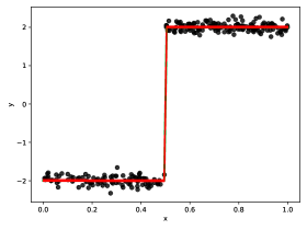
(b) XBART (RMSE: 0.0982)

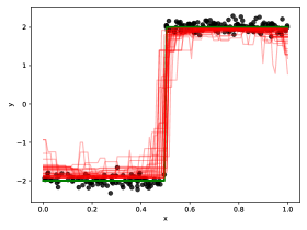
(c) SGLB (RMSE: 0.3014)

Figure 6: Step function. The variational soft decision tree (VST) can fit this non-smooth function. The plot for the VST was generated with the linear leaf model.

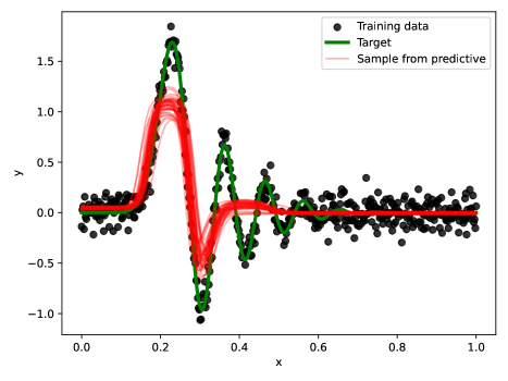
(a) VST (RMSE: 0.2346)

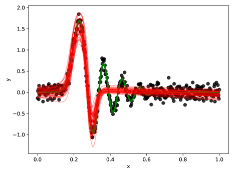
(b) VSGBM (RMSE: 0.2534)

(c) XBART (RMSE: 0.1186)

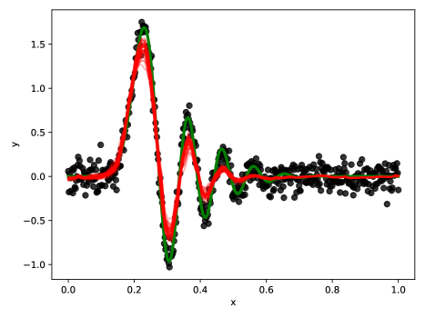
(d) SGLB (RMSE: 0.1503)

Figure 7: Daubechies wavelet. The variational soft tree (VST) and variational soft GBM (VSGBM) underfit this complex function.

References

- Abdullah et al., (2022) Abdullah, A., Hassan, M., and Mustafa, Y. (2022). A review on Bayesian deep learning in healthcare: Applications and challenges. IEEE Access, 10:1–1.
- Ahmetoğlu et al., (2018) Ahmetoğlu, A., İrsoy, O., and Alpaydın, E. (2018). Convolutional soft decision trees. In Kůrková, V., Manolopoulos, Y., Hammer, B., Iliadis, L., and Maglogiannis, I., editors, Artificial Neural Networks and Machine Learning – ICANN 2018, pages 134–141, Cham. Springer International Publishing.
- Bew et al., (2019) Bew, D., Harvey, C. R., Ledford, A., Radnor, S., and Sinclair, A. (2019). Modeling analysts’ recommendations via Bayesian machine learning. The Journal of Financial Data Science, 1(1):75–98.
- Bishop and Svensen, (2012) Bishop, C. M. and Svensen, M. (2012). Bayesian hierarchical mixtures of experts.
- Blundell et al., (2015) Blundell, C., Cornebise, J., Kavukcuoglu, K., and Wierstra, D. (2015). Weight uncertainty in neural networks.
- Bojer and Meldgaard, (2021) Bojer, C. S. and Meldgaard, J. P. (2021). Kaggle forecasting competitions: An overlooked learning opportunity. International Journal of Forecasting, 37(2):587–603.
- Borisov et al., (2021) Borisov, V., Leemann, T., Seßler, K., Haug, J., Pawelczyk, M., and Kasneci, G. (2021). Deep neural networks and tabular data: A survey.
- Bradbury et al., (2018) Bradbury, J., Frostig, R., Hawkins, P., Johnson, M. J., Leary, C., Maclaurin, D., Necula, G., Paszke, A., VanderPlas, J., Wanderman-Milne, S., and Zhang, Q. (2018). JAX: Composable transformations of Python+NumPy programs.
- Chen and Guestrin, (2016) Chen, T. and Guestrin, C. (2016). XGBoost: A scalable tree boosting system. In Proceedings of the 22nd ACM SIGKDD International Conference on Knowledge Discovery and Data Mining, San Francisco, CA, USA, August 13-17, 2016, pages 785–794.
- Chipman et al., (1998) Chipman, H. A., George, E. I., and McCulloch, R. E. (1998). Bayesian cart model search. Journal of the American Statistical Association, 93(443):935–948.
- Clements et al., (2020) Clements, J. M., Xu, D., Yousefi, N., and Efimov, D. (2020). Sequential deep learning for credit risk monitoring with tabular financial data.
- Cobb and Jalaian, (2020) Cobb, A. D. and Jalaian, B. (2020). Scaling Hamiltonian Monte Carlo inference for Bayesian neural networks with symmetric splitting.
- Coppens et al., (2019) Coppens, Y., Efthymiadis, K., Lenaerts, T., and Nowé, A. (2019). Distilling deep reinforcement learning policies in soft decision trees. In IJCAI 2019.
- Deisenroth and Rasmussen, (2011) Deisenroth, M. and Rasmussen, C. (2011). Pilco: A model-based and data-efficient approach to policy search. pages 465–472.
- Dempster et al., (1977) Dempster, A. P., Laird, N. M., and Rubin, D. B. (1977). Maximum likelihood from incomplete data via the EM algorithm. JOURNAL OF THE ROYAL STATISTICAL SOCIETY, SERIES B, 39(1):1–38.
- Dua and Graff, (2017) Dua, D. and Graff, C. (2017). UCI machine learning repository.
- Ebbehoj et al., (2021) Ebbehoj, A., Thunbo, M., Andersen, O. E., Glindtvad, M. V., and Hulman, A. (2021). Transfer learning for non-image data in clinical research: a scoping review. medRxiv.
- Feng et al., (2020) Feng, J., Xu, Y.-X., Jiang, Y., and Zhou, Z.-H. (2020). Soft gradient boosting machine.
- Flam-Shepherd, (2017) Flam-Shepherd, D. (2017). Mapping Gaussian process priors to Bayesian neural networks.
- Fortuin et al., (2021) Fortuin, V., Garriga-Alonso, A., Ober, S. W., Wenzel, F., Rätsch, G., Turner, R. E., van der Wilk, M., and Aitchison, L. (2021). Bayesian neural network priors revisited.
- Freund and Schapire, (1997) Freund, Y. and Schapire, R. E. (1997). A decision-theoretic generalization of on-line learning and an application to boosting. Journal of Computer and System Sciences, 55(1):119–139.
- Friedman, (2001) Friedman, J. H. (2001). Greedy function approximation: A gradient boosting machine. The Annals of Statistics, 29(5):1189 – 1232.
- Frosst and Hinton, (2017) Frosst, N. and Hinton, G. (2017). Distilling a neural network into a soft decision tree.
- Goldberg et al., (2001) Goldberg, K., Roeder, T., Gupta, D., and Perkins, C. (2001). Eigentaste: A constant time collaborative filtering algorithm. Information Retrieval, 4:133–151.
- Gonzalvez et al., (2019) Gonzalvez, J., Lezmi, E., Roncalli, T., and Xu, J. (2019). Financial applications of Gaussian processes and Bayesian optimization.
- Graf et al., (2011) Graf, F., Kriegel, H.-P., Schubert, M., Pölsterl, S., and Cavallaro, A. (2011). 2D image registration in CT images using radial image descriptors. Medical image computing and computer-assisted intervention : MICCAI … International Conference on Medical Image Computing and Computer-Assisted Intervention, 14 Pt 2:607–14.
- Guo et al., (2017) Guo, C., Pleiss, G., Sun, Y., and Weinberger, K. Q. (2017). On calibration of modern neural networks. In International conference on machine learning, pages 1321–1330. PMLR.
- He and Hahn, (2020) He, J. and Hahn, P. R. (2020). Stochastic tree ensembles for regularized nonlinear regression.
- Hennigan et al., (2020) Hennigan, T., Cai, T., Norman, T., and Babuschkin, I. (2020). Haiku: Sonnet for JAX.
- Hoang and Wiegratz, (2021) Hoang, D. and Wiegratz, K. (2021). Machine learning methods in finance: Recent applications and prospects.
- Hoffman et al., (2013) Hoffman, M. D., Blei, D. M., Wang, C., and Paisley, J. (2013). Stochastic variational inference. Journal of Machine Learning Research, 14(40):1303–1347.
- Immer et al., (2020) Immer, A., Korzepa, M., and Bauer, M. (2020). Improving predictions of Bayesian neural nets via local linearization.
- Irsoy et al., (2012) Irsoy, O., Yildiz, O., and Alpaydın, E. (2012). Soft decision trees. pages 1819–1822.
- Jordan and Jacobs, (1993) Jordan, M. and Jacobs, R. (1993). Hierarchical mixtures of experts and the EM algorithm. In Proceedings of 1993 International Conference on Neural Networks (IJCNN-93-Nagoya, Japan), volume 2, pages 1339–1344 vol.2.
- Kingma and Ba, (2014) Kingma, D. P. and Ba, J. (2014). Adam: A method for stochastic optimization.
- Kingma and Welling, (2013) Kingma, D. P. and Welling, M. (2013). Auto-encoding variational Bayes.
- Kirsch et al., (2019) Kirsch, A., van Amersfoort, J., and Gal, Y. (2019). Batchbald: Efficient and diverse batch acquisition for deep Bayesian active learning.
- Kompa et al., (2021) Kompa, B., Snoek, J., and Beam, A. (2021). Second opinion needed: communicating uncertainty in medical machine learning. npj Digital Medicine, 4.
- Kontschieder et al., (2015) Kontschieder, P., Fiterau, M., Criminisi, A., and Rota Bulò, S. (2015). Deep neural decision forests. pages 1467–1475.
- Krause et al., (2006) Krause, A., Guestrin, C., Gupta, A., and Kleinberg, J. (2006). Near-optimal sensor placements: Maximizing information while minimizing communication cost. In 2006 5th International Conference on Information Processing in Sensor Networks, pages 2–10.
- Krishnan et al., (2020) Krishnan, R., Subedar, M., and Tickoo, O. (2020). Specifying weight priors in Bayesian deep neural networks with empirical Bayes. Proceedings of the AAAI Conference on Artificial Intelligence, 34(04):4477–4484.
- Kristiadi et al., (2020) Kristiadi, A., Hein, M., and Hennig, P. (2020). Being Bayesian, even just a bit, fixes overconfidence in ReLU networks.
- Linero and Yang, (2017) Linero, A. R. and Yang, Y. (2017). Bayesian regression tree ensembles that adapt to smoothness and sparsity.
- Liu et al., (2021) Liu, Z., Pavao, A., Xu, Z., Escalera, S., Ferreira, F., Guyon, I., Hong, S., Hutter, F., Ji, R., Jacques Junior, J. C. S., Li, G., Lindauer, M., Luo, Z., Madadi, M., Nierhoff, T., Niu, K., Pan, C., Stoll, D., Treguer, S., Wang, J., Wang, P., Wu, C., Xiong, Y., Zela, A., and Zhang, Y. (2021). Winning solutions and post-challenge analyses of the ChaLearn AutoDL challenge 2019. IEEE Transactions on Pattern Analysis and Machine Intelligence.
- Luo et al., (2021) Luo, H., Cheng, F., Yu, H., and Yi, Y. (2021). SDTR: Soft decision tree regressor for tabular data. IEEE Access, 9:55999–56011.
- Ma and Hernández-Lobato, (2021) Ma, C. and Hernández-Lobato, J. M. (2021). Functional variational inference based on stochastic process generators. In Ranzato, M., Beygelzimer, A., Dauphin, Y., Liang, P., and Vaughan, J. W., editors, Advances in Neural Information Processing Systems, volume 34, pages 21795–21807. Curran Associates, Inc.
- Maia et al., (2022) Maia, M., Murphy, K., and Parnell, A. C. (2022). GP-BART: A novel Bayesian additive regression trees approach using Gaussian processes. arXiv e-prints, page arXiv:2204.02112.
- Malinin et al., (2020) Malinin, A., Prokhorenkova, L., and Ustimenko, A. (2020). Uncertainty in gradient boosting via ensembles.
- Mitros and Namee, (2019) Mitros, J. and Namee, B. M. (2019). On the validity of Bayesian neural networks for uncertainty estimation.
- Mukhoti et al., (2021) Mukhoti, J., Kirsch, A., van Amersfoort, J., Torr, P. H. S., and Gal, Y. (2021). Deep deterministic uncertainty: A simple baseline.
- Mustafa and Rahimi Azghadi, (2021) Mustafa, A. and Rahimi Azghadi, M. (2021). Automated machine learning for healthcare and clinical notes analysis. Computers, 10(2).
- Niculescu-Mizil and Caruana, (2012) Niculescu-Mizil, A. and Caruana, R. A. (2012). Obtaining calibrated probabilities from boosting.
- Pratola et al., (2017) Pratola, M., Chipman, H., George, E., and McCulloch, R. (2017). Heteroscedastic BART using multiplicative regression trees.
- Riquelme et al., (2018) Riquelme, C., Tucker, G., and Snoek, J. (2018). Deep Bayesian bandits showdown: An empirical comparison of Bayesian deep networks for Thompson sampling.
- Shwartz-Ziv and Armon, (2022) Shwartz-Ziv, R. and Armon, A. (2022). Tabular data: Deep learning is not all you need. Information Fusion, 81:84–90.
- Springenberg et al., (2016) Springenberg, J. T., Klein, A., Falkner, S., and Hutter, F. (2016). Bayesian optimization with robust Bayesian neural networks. In Lee, D., Sugiyama, M., Luxburg, U., Guyon, I., and Garnett, R., editors, Advances in Neural Information Processing Systems, volume 29. Curran Associates, Inc.
- Swiatkowski et al., (2020) Swiatkowski, J., Roth, K., Veeling, B. S., Tran, L., Dillon, J. V., Snoek, J., Mandt, S., Salimans, T., Jenatton, R., and Nowozin, S. (2020). The k-tied normal distribution: A compact parameterization of Gaussian mean field posteriors in Bayesian neural networks.
- Thompson, (1933) Thompson, W. R. (1933). On the likelihood that one unknown probability exceeds another in view of the evidence of two samples. Biometrika, 25(3-4):285–294.
- Tomczak et al., (2020) Tomczak, M., Swaroop, S., and Turner, R. (2020). Efficient low rank Gaussian variational inference for neural networks. In Larochelle, H., Ranzato, M., Hadsell, R., Balcan, M., and Lin, H., editors, Advances in Neural Information Processing Systems, volume 33, pages 4610–4622. Curran Associates, Inc.
- Tran et al., (2015) Tran, D., Ranganath, R., and Blei, D. M. (2015). The variational Gaussian process.
- Ueda and Ghahramani, (2002) Ueda, N. and Ghahramani, Z. (2002). Bayesian model search for mixture models based on optimizing variational bounds. Neural Networks, 15(10):1223–1241.
- Ustimenko and Prokhorenkova, (2020) Ustimenko, A. and Prokhorenkova, L. (2020). SGLB: Stochastic gradient Langevin boosting.
- Vladimirova et al., (2018) Vladimirova, M., Verbeek, J., Mesejo, P., and Arbel, J. (2018). Understanding priors in Bayesian neural networks at the unit level.
- Waterhouse et al., (1995) Waterhouse, S., MacKay, D., and Robinson, A. (1995). Bayesian methods for mixtures of experts. In Touretzky, D., Mozer, M., and Hasselmo, M., editors, Advances in Neural Information Processing Systems, volume 8. MIT Press.
- Welling and Teh, (2011) Welling, M. and Teh, Y. W. (2011). Bayesian learning via stochastic gradient Langevin dynamics. In Proceedings of the 28th International Conference on International Conference on Machine Learning, ICML’11, page 681–688, Madison, WI, USA. Omnipress.