Boosting the Power of Kernel Two-Sample Tests

Abstract.

The kernel two-sample test based on the maximum mean discrepancy (MMD) is one of the most popular methods for detecting differences between two distributions over general metric spaces. In this paper we propose a method to boost the power of the kernel test by combining MMD estimates over multiple kernels using their Mahalanobis distance. We derive the asymptotic null distribution of the proposed test statistic and use a multiplier bootstrap approach to efficiently compute the rejection region. The resulting test is universally consistent and, since it is obtained by aggregating over a collection of kernels/bandwidths, is more powerful in detecting a wide range of alternatives in finite samples. We also derive the distribution of the test statistic for both fixed and local contiguous alternatives. The latter, in particular, implies that the proposed test is statistically efficient, that is, it has non-trivial asymptotic (Pitman) efficiency. Extensive numerical experiments are performed on both synthetic and real-world datasets to illustrate the efficacy of the proposed method over single kernel tests. Our asymptotic results rely on deriving the joint distribution of MMD estimates using the framework of multiple stochastic integrals, which is more broadly useful, specifically, in understanding the efficiency properties of recently proposed adaptive MMD tests based on kernel aggregation.

1. Introduction

Given two probability distributions $P$ and $Q$ on a separable metric space $\mathcal{X}$, the two-sample problem is to test the hypothesis:

$$H_{0}:P=Q\quad\text{ versus }\quad H_{1}:P\neq Q,$$ (1.1)

based on i.i.d. samples $\mathscr{X}_{m}:=\{X_{1},X_{2},\ldots,X_{m}\}\text{ and }\mathscr{Y}_{n}:=\{Y_{1},Y_{2},\ldots,Y_{n}\}$ from the distributions $P$ and $Q$, respectively. This is a classical problem that has been extensively studied, especially in the parametric regime, where the data is assumed to have certain low-dimensional functional forms. However, parametric methods often perform poorly for misspecified models, especially when the number of nuisance parameters is large, and for non-Euclidean data. This necessitates the development of non-parametric methods, which make minimal distributional assumptions on the data, but remain powerful for a wide class of alternatives.

For univariate data, there are several well-known nonparametric tests such as the two-sample Kolmogorov–Smirnoff (KS) maximum deviation test [59], the Wald-Wolfwotiz runs test [65], the rank-sum test [46, 67], and the Cramér-von Mises test [1]. Efforts to generalize these univariate methods to higher dimensions date back to Weiss [66] and Bickel [9]. Thereafter, several nonparametric methods for multivariate two-sample testing have been proposed over the years. These include tests based on geometric graphs [19, 28, 54, 25, 52, 11, 7, 27, 26, 10, 53], tests based on data-depth [42, 43], the energy distance test [61, 62, 5, 3, 63], kernel maximum mean discrepancy (MMD) tests [23, 22, 24, 60, 13, 48, 49, 68, 58, 56], ball divergence [47, 4], projection-averaging [33], classifier-based tests [44, 34], among others. Recently, distribution-free versions of the energy distance/kernel tests have been proposed by Deb and Sen [14] and Deb et al. [15], using the emerging theory of multivariate ranks based on optimal transport.

Among the aforementioned methods kernel-based tests have emerged as a powerful technique for detecting distributional differences on general domains. The basic idea is to quantify the discrepancy between the two distributions $P$ and $Q$ in terms of the largest difference in expectation between $f(X)$ and $f(Y)$, for $X\sim P$ and $Y\sim Q$, over functions $f$ in the unit ball of a reproducing kernel Hilbert space (RKHS) defined on $\mathcal{X}$. This is called the maximum mean discrepancy (MMD) between the distributions $P$ and $Q$ (see (2.1) for the precise definition), which can be conveniently estimated from the data in terms of the pairwise kernel dissimilarities (see Section 2.1 for details). Another useful property of the MMD is that it takes value zero if and only if the distributions $P$ and $Q$ are the same. Consequently, the test which rejects $H_{0}$ for large values of the estimated MMD is universally consistent (the power of the test converges to 1 as the sample size increases) for the hypothesis (1.1) (see Gretton et al. [23] for further details).

Although the kernel two-sample test is widely used and has found numerous applications, it often performs poorly for high-dimensional problems [48] and its empirical performance depends heavily on the choice of the kernel. Kernels are usually parametrized by their bandwidths, and the most popular strategy for choosing the kernel bandwidth is the median heuristics, where the bandwidth is chosen to be the median of the pairwise distances of the pooled sample [23]. Despite its popularity there is limited understanding of the median heuristic and empirical results demonstrate that the median heuristic performs poorly when differences between the 2 distributions occur at a scale that differs significantly from the median of the interpoint distances [24]. Another approach is to split the data and estimate the kernel by maximizing an approximate empirical power on the held-out data [41, 24]. This, however, can lead to loss in power for smaller sample sizes. (For a discussion of other related methods see Section 9.)

In this paper we propose a strategy for augmenting the power of the classical (single) kernel two-sample test by borrowing strengths from multiple kernels. Specifically, we propose a new test statistic which combines MMD estimates from $r\geq 1$ kernels using their sample Mahalanobis distance. The advantage of aggregating across a collection of kernels/bandwidths is that the test can simultaneously deal with cases which require both small and large bandwidths, and, hence, detect both global and local differences more effectively. To understand the asymptotic properties of the test we derive the joint distribution of the vector of MMD estimates under $H_{0}$, which can be described using bivariate stochastic integrals, and, as a consequence, derive the asymptotic distribution of the Mahalanobis aggregated MMD (MMMD) statistic under $H_{0}$ (Section 3). Moreover, using the kernel Gram matrix representation we develop a multiplier bootstrap approach that allows us to efficiently compute the rejection threshold for the MMMD statistic and show that the resulting test is universally consistent (Section 4). Next, we establish the asymptotic (Pitman) efficiency of the proposed test by deriving its power against local alternatives in the well-known contamination model (Section 5). In Section 6 we derive the joint distribution of MMD estimates and, consequently, that of the MMMD statistic, under the alternative.

In Section 7 we perform extensive simulations to compare our MMMD based test with various single kernel MMD tests (with bandwidths chosen based on the median heuristic). The experiments show that the MMMD method outperforms the single kernel tests and also the graph-based Friedman-Rafsky test [19] across a range alternatives and dimensions, showcasing the efficacy of our aggregation method. In Section 8 we apply the proposed method to compare images of digits in the noisy MNIST dataset. The MMMD effectively distinguishes different digits for significantly more noisy images compared to its single kernel counterparts, again illustrating the advantage of using multiple kernels.

Our results on the joint distribution for multiple kernels are also more broadly useful in understanding the asymptotic properties of general aggregation strategies. To demonstrate this, in Section 9, we propose an asymptotic implementation of the adaptive MMD test recently proposed in [55], and derive its asymptotic local power. Numerical results comparing the MMMD method and the aforementioned adaptive test are also reported. The codes for all the experiments can be found in the Github repository https://github.com/anirbanc96/MMMD-boost-kernel-two-sample.

2. Kernel Maximum Mean Discrepancy and Mahalanobis Aggregation

We begin by recalling the fundamentals of the kernel two-sample test as introduced in Gretton et al. [23] in Section 2.1. Then in Section 2.2 we describe our proposed test statistic obtained by combining multiple kernels.

2.1. Kernel Maximum Mean Discrepancy

Suppose $\mathcal{X}$ is a separable metric space and $\mathscr{B}(\mathcal{X})$ is the sigma-algebra generated by the open sets of $\mathcal{X}$. Denote by $\mathcal{P}(\mathcal{X})$ the collection of all probability distributions on $(\mathcal{X},\mathscr{B}(\mathcal{X}))$. Suppose $P,Q\in\mathcal{P}(X)$ and $X\sim P$ and $Y\sim Q$ be random variables distributed as $P$ and $Q$, respectively. Throughout we will assume that $P$ and $Q$ are non-atomic. The maximum mean discrepancy (MMD) between $P$ and $Q$ is defined as

$$\mathrm{MMD}\left[\mathcal{F},P,Q\right]=\sup_{f\in\mathcal{F}}\left\{\mathbb{E}_{X\sim P}[f(X)]-\mathbb{E}_{Y\sim Q}[f(Y)]\right\},$$ (2.1)

where $\mathcal{F}$ is the unit ball of a reproducing kernel Hilbert space (RKHS) $\mathcal{H}$ defined on $\mathcal{X}$ [2]. Since $\mathcal{H}$ is an RKHS, for every $x\in\mathcal{X}$ the evaluation map operator $\eta_{x}:\mathcal{H}\rightarrow\mathbb{R}$ given $\eta_{x}(f)=f(x)$ is continuous. Thus, by the Riesz representation theorem [50, Theorem II.4] for each $x\in\mathcal{X}$ there is a feature mapping $\psi_{x}\in\mathcal{H}$ such that $f(x)=\langle f,\psi_{x}\rangle_{\mathcal{H}}$, for every $f\in\mathcal{H}$, where $\langle\cdot,\cdot\rangle_{\mathcal{H}}$ is the inner product in $\mathcal{H}$. The feature mapping takes the canonical form $\psi_{x}(\cdot)={\mathsf{K}}(x,\cdot)$, where ${\mathsf{K}}:\mathcal{X}\times\mathcal{X}\rightarrow\mathbb{R}$ is a positive definite kernel. This, in particular, implies that ${\mathsf{K}}(x,y)=\langle\psi(x),\psi(y)\rangle_{\mathcal{H}}$. Extending the notion of feature map, an element $\mu_{P}\in\mathcal{H}$ is defined to be the mean embedding of $P\in\mathcal{P}\left(\mathcal{X}\right)$ if

$$\langle f,\mu_{P}\rangle_{\mathcal{H}}=\mathbb{E}_{X\sim P}[f(X)],$$ (2.2)

for all $f\in\mathcal{H}$. By the canonical form of the feature map it follows that

$$\mu_{P}(t):=\int_{\mathcal{X}}\psi_{t}(x)\mathrm{d}P(x)=\mathbb{E}_{X\sim P}[\psi_{t}(X)]=\mathbb{E}_{X\sim P}[{\mathsf{K}}(t,X)].$$ (2.3)

Throughout we will make the following assumption:

Assumption 2.1.

The kernel ${\mathsf{K}}:\mathcal{X}\times\mathcal{X}\rightarrow\mathbb{R}$ satisfies the following:

• $\mathbb{E}_{X\sim P}[{\mathsf{K}}(X,X)^{\frac{1}{2}}]<\infty$ and $\mathbb{E}_{Y\sim Q}[{\mathsf{K}}(Y,Y)^{\frac{1}{2}}]<\infty$.

• ${\mathsf{K}}$ is characteristic, that is, the mean embedding $\mu:\mathcal{P}(\mathcal{X})\rightarrow\mathcal{H}$ is a one-to-one (injective) function.

Assumption 2.1 ensures that $\mu_{P},\mu_{Q}\in\mathcal{H}$ and MMD defines a metric on $\mathcal{P}(\mathcal{X})$. Then the MMD can be expressed as the distance between mean embeddings in $\mathcal{H}$ (see [23, Lemma 4]):

$$\mathrm{MMD}^{2}\left[\mathcal{F},P,Q\right]=\left\|\mu_{P}-\mu_{Q}\right\|_{\mathcal{H}}^{2},$$ (2.4)

where $\|\cdot\|_{\mathcal{H}}$ is the norm corresponding to the inner product $\langle\cdot,\cdot\rangle_{\mathcal{H}}$. This implies $\mathrm{MMD}^{2}\left[\mathcal{F},P,Q\right]=0$ if and only if $P=Q$. Expanding the square in (2.4) and using the representation in (2.3) it follows that (see [23, Lemma 6] for details)

$$\mathrm{MMD}^{2}\left[\mathcal{F},P,Q\right]=\mathbb{E}_{X,X^{\prime}\sim P}[{\mathsf{K}}(X,X^{\prime})]+\mathbb{E}_{Y,Y^{\prime}\sim Q}[{\mathsf{K}}(Y,Y^{\prime})]-2\mathbb{E}_{X\sim P,Y\sim Q}[{\mathsf{K}}(X,Y)].$$

Therefore, based on i.i.d. observations $\mathscr{X}_{m}:=\{X_{1},X_{2},\ldots,X_{m}\}\text{ and }\mathscr{Y}_{n}:=\{Y_{1},Y_{2},\ldots,Y_{n}\}$, a natural unbiased estimate of $\mathrm{MMD}^{2}\left[\mathcal{F},P,Q\right]$ is given by,

$$\mathrm{MMD}^{2}\left[{\mathsf{K}},\mathscr{X}_{m},\mathscr{Y}_{n}\right]=\mathcal{W}_{\mathscr{X}_{m}}+\mathcal{W}_{\mathscr{Y}_{n}}-2\mathcal{B}_{\mathscr{X}_{m},\mathscr{Y}_{n}},$$ (2.5)

where

$$\mathcal{W}_{\mathscr{X}_{m}}:=\frac{1}{m(m-1)}\sum_{1\leq i\neq j\leq m}{\mathsf{K}}\left(X_{i},X_{j}\right)\text{ and }\mathcal{W}_{\mathscr{Y}_{n}}:=\frac{1}{n(n-1)}\sum_{1\leq i\neq j\leq n}{\mathsf{K}}\left(Y_{i},Y_{j}\right)$$ (2.6)

is the average of the kernel dissimilarities within the samples in $\mathscr{X}_{m}$ and $\mathscr{Y}_{n}$, respectively, and

$$\mathcal{B}_{\mathscr{X}_{m},\mathscr{Y}_{n}}:=\frac{1}{mn}\sum_{i=1}^{m}\sum_{j=1}^{n}{\mathsf{K}}\left(X_{i},Y_{j}\right)$$ (2.7)

is the average of the kernel dissimilarities between the samples in $\mathscr{X}_{m}$ and $\mathscr{Y}_{n}$. In the asymptotic regime where $N:=m+n\rightarrow\infty$ such that

$$\frac{m}{m+n}\rightarrow\rho\in(0,1),$$ (2.8)

$\mathrm{MMD}^{2}[{\mathsf{K}},\mathscr{X}_{m},\mathscr{Y}_{n}]$ is a consistent estimate of $\mathrm{MMD}^{2}\left[\mathcal{F},P,Q\right]$ (see [23, Theorem 7]), that is,

$$\mathrm{MMD}^{2}[{\mathsf{K}},\mathscr{X}_{m},\mathscr{Y}_{n}]\stackrel{{\scriptstyle P}}{{\to}}\mathrm{MMD}^{2}\left[\mathcal{F},P,Q\right].$$ (2.9)

Hence, the test which rejects $H_{0}$ in (1.1) for large values of $\mathrm{MMD}^{2}\left[{\mathsf{K}},\mathscr{X}_{m},\mathscr{Y}_{n}\right]$ is universally consistent.

2.2. Aggregating Multiple Kernels

Fix $r\geq 1$ and suppose ${\mathsf{K}}_{1},{\mathsf{K}}_{2},\ldots,{\mathsf{K}}_{r}$ be $r$ distinct kernels each of which satisfy Assumption 2.1. Denote the vector of MMD estimates as

$$\mathrm{MMD}^{2}\left[\mathcal{K},\mathscr{X}_{m},\mathscr{Y}_{n}\right]=\left(\mathrm{MMD}^{2}[{\mathsf{K}}_{1},\mathscr{X}_{m},\mathscr{Y}_{n}],\cdots,\mathrm{MMD}^{2}[{\mathsf{K}}_{r},\mathscr{X}_{m},\mathscr{Y}_{n}]\right)^{\top},$$ (2.10)

where $\mathcal{K}:=\{{\mathsf{K}}_{1},{\mathsf{K}}_{2},\ldots,{\mathsf{K}}_{r}\}$. In this paper we propose a new test statistic that combines the contributions of the different kernels using the Mahalanobis distance of the vector $\mathrm{MMD}^{2}\left[\mathcal{K},\mathscr{X}_{m},\mathscr{Y}_{n}\right]$ as follows:

$$\left(\mathrm{MMD}^{2}\left[\mathcal{K},\mathscr{X}_{m},\mathscr{Y}_{n}\right]\right)^{\top}\bm{S}^{-1}\left(\mathrm{MMD}^{2}\left[\mathcal{K},\mathscr{X}_{m},\mathscr{Y}_{n}\right]\right),$$ (2.11)

where is $\bm{S}$ is a consistent estimate of the limiting covariance matrix of $\mathrm{MMD}^{2}\left[\mathcal{K},\mathscr{X}_{m},\mathscr{Y}_{n}\right]$ under $H_{0}$ (which we denote by ${\bm{\Sigma}}_{H_{0}}=((\sigma_{ab}))_{1\leq a,b\leq r}$). Note that adjusting by the covariance matrix $\bm{S}$ brings the contributions of the individual MMD estimates in the same scale and by selecting a range of kernels/bandwidths in $\mathcal{K}$ one can detect more fine-grained deviations from $H_{0}$, leading to significant power improvements as in will be seen in Section 7. (In Appendix E we present general conditions under which $\bm{\Sigma}_{H_{0}}$ is invertible, which, in particular, hold for the any collection of Gaussian or Laplace kernels.)

In Corollary 3.1 we compute

$$\sigma_{ab} :=\lim_{N\rightarrow\infty}(m+n)^{2}\left(\operatorname{Cov}_{H_{0}}\left[\mathrm{MMD}^{2}\left[\mathcal{K},\mathscr{X}_{m},\mathscr{Y}_{n}\right]\right]\right)_{ab}$$ (2.12)

$$=\frac{2}{\rho^{2}(1-\rho)^{2}}\mathbb{E}_{X,X^{\prime}\sim P}\left[{\mathsf{K}}_{a}^{\circ}(X,X^{\prime}){\mathsf{K}}_{b}^{\circ}(X,X^{\prime})\right],$$

where

$${\mathsf{K}}_{a}^{\circ}(x,y)={\mathsf{K}}_{a}(x,y)-\mathbb{E}_{X\sim P}{\mathsf{K}}_{a}(X,y)-\mathbb{E}_{X^{\prime}\sim P}{\mathsf{K}}_{a}(x,X^{\prime})+\mathbb{E}_{X,X^{\prime}\sim P}{\mathsf{K}}_{a}(X,X^{\prime})$$ (2.13)

is the centered version of the kernel ${\mathsf{K}}_{a}$, for $1\leq a\leq r$. Therefore, a natural empirical estimate of $\bm{\Sigma}_{H_{0}}$ is the given by $\hat{\bm{\Sigma}}=((\hat{\sigma}_{ab}))_{1\leq a,b\leq r}$, where

$$\hat{\sigma}_{ab} =\frac{2}{\hat{\rho}^{2}(1-\hat{\rho})^{2}}\cdot\frac{1}{m^{2}}\sum_{1\leq i,j\leq m}\hat{\mathsf{K}}_{a}^{\circ}(X_{i},X_{j})\hat{\mathsf{K}}_{b}^{\circ}(X_{i},X_{j}),$$ (2.14)

with

$$\hat{\mathsf{K}}_{a}^{\circ}(x,y)={\mathsf{K}}_{a}(x,y)-\frac{1}{m}\sum_{u=1}^{m}{\mathsf{K}}_{a}(X_{u},y)-\frac{1}{m}\sum_{v=1}^{m}{\mathsf{K}}_{a}(x,X_{v})+\frac{1}{m^{2}}\sum_{1\leq u,v\leq m}{\mathsf{K}}_{a}(X_{u},X_{v})$$ (2.15)

being the empirical analogue of ${\mathsf{K}}_{a}^{\circ}$ and $\hat{\rho}=\frac{m}{m+n}$. Therefore, choosing $\bm{S}=\hat{\bm{\Sigma}}$ in (2.11) we define the Mahalanobis aggregated MMD (MMMD) statistic as follows:

$$T_{m,n}:=\left(\mathrm{MMD}^{2}\left[\mathcal{K},\mathscr{X}_{m},\mathscr{Y}_{n}\right]\right)^{\top}\hat{\bm{\Sigma}}^{-1}\left(\mathrm{MMD}^{2}\left[\mathcal{K},\mathscr{X}_{m},\mathscr{Y}_{n}\right]\right).$$ (2.16)

In Corollary 3.1 we show that $\hat{\bm{\Sigma}}\stackrel{{\scriptstyle P}}{{\to}}\bm{\Sigma}_{H_{0}}$, hence (2.9) implies that

$$T_{m,n}\stackrel{{\scriptstyle P}}{{\to}}\left(\mathrm{MMD}^{2}\left[\mathcal{K},P,Q\right]\right)^{\top}\bm{\Sigma}^{-1}_{H_{0}}\left(\mathrm{MMD}^{2}\left[\mathcal{K},P,Q\right]\right):=T_{\mathcal{K}}.$$ (2.17)

Note that $T_{\mathcal{K}}=0$ under $H_{0}$ and $T_{\mathcal{K}}>0$ whenever $P\neq Q$. Hence, a test rejecting $H_{0}$ for ‘large’ values of $T_{m,n}$ will be universally consistent. However, to construct a test based on $T_{m,n}$ we need to chose a cut-off (rejection region) based on the data. The first step towards this to derive the limiting null distribution of $\mathrm{MMD}^{2}\left[\mathcal{K},\mathscr{X}_{m},\mathscr{Y}_{n}\right]$. This is discussed in Section 3.

3. Asymptotic Null Distribution

In this section we derive the limiting distribution of the vector of MMD estimates (2.10) under $H_{0}$ and, consequently, that of the proposed statistic $T_{m,n}$. In Section 3.1 we recall the definition and basic properties of multiple Weiner-Itô stochastic integrals as presented in Itô [30]. Using this framework, we derive the joint asymptotic null distribution of (2.10) in Section 3.2.

3.1. Multiple Weiner-Itô Stochastic Integrals

Recall that $\mathcal{X}$ is a separable metric space, $\mathscr{B}(\mathcal{X})$ is the sigma-algebra generated by the open sets of $\mathcal{X}$, and $P$ is a non-atomic probability measure on $\mathcal{X}$. We denote this probability space by $(\mathcal{X},\mathscr{B}(\mathcal{X}),P)$.

Definition 3.1.

A Gaussian stochastic measure on $(\mathcal{X},\mathscr{B}(\mathcal{X}),P)$ is a collection of random variables $\{\mathcal{Z}_{P}(A):A\in\mathscr{B}(\mathcal{X})\}$ defined on a common probability space $(\Omega,\mathcal{F},\mu)$ such that the following hold:

• $\mathcal{Z}_{P}(A)\sim\mathcal{N}(0,P(A))$, for all $A\in\mathscr{B}(\mathcal{X})$.

• For any finite collection of disjoint sets $A_{1},\cdots,A_{t}\in\mathscr{B}(\mathcal{X})$, the random variables $\{\mathcal{Z}_{P}(A_{1}),\mathcal{Z}_{P}(A_{2}),\ldots,\mathcal{Z}_{P}(A_{t})\}$ are independent and

  $$\mathcal{Z}_{P}\left(\bigcup_{s=1}^{t}A_{s}\right)=\sum_{s=1}^{t}\mathcal{Z}_{P}(A_{s}).$$

For $d\geq 1$, denote by $L^{2}(\mathcal{X}^{d},\mathscr{B}(\mathcal{X}^{d}),P^{d})$ the space of measurable functions $f:\mathcal{X}^{d}\rightarrow\mathbb{R}$ such that

$$\|f\|^{2}:=\int_{\mathcal{X}^{d}}|f(x_{1},x_{2},\ldots,x_{d})|^{2}\mathrm{d}P(x_{1})\mathrm{d}P(x_{2})\ldots,\mathrm{d}P(x_{d})<\infty.$$

Define $\mathcal{E}_{d}\subseteq L^{2}(\mathcal{X}^{d},\mathscr{B}(\mathcal{X}^{d}),P^{d})$ as the set of all elementary functions having the form

$$f(t_{1},t_{2},\ldots,t_{d})=\sum_{1\leq i_{1},i_{2},\ldots,i_{d}\leq m}a_{i_{1},i_{2},\ldots,i_{d}}\bm{1}\{(t_{1},t_{2},\ldots,t_{d})\in A_{i_{1}}\times\cdots\times A_{i_{d}}\},$$ (3.1)

where $A_{1},A_{2},\ldots,A_{m}\in\mathscr{B}(\mathcal{X})$ are pairwise disjoint and $a_{i_{1},i_{2},\ldots,i_{d}}$ is zero if two indices are equal. The multiple Weiner-Itô integral for functions in $\mathcal{E}_{d}$ is defined as follows:

Definition 3.2.

(Multiple Weiner-Itô integral for elementary functions) The $d$-dimensional Weiner-Itô stochastic integral, with respect to the Gaussian stochastic measure $\{Z_{P}(A),A\in\mathscr{B}(\mathcal{X})\}$, for the function $f\in\mathcal{E}_{d}$ in (3.1) is defined as

$$I_{d}(f):=\int_{\mathcal{X}^{d}}f(x_{1},x_{2},\ldots,x_{d})\prod_{a=1}^{d}\mathrm{d}\mathcal{Z}_{P}(x_{a}):=\sum_{1\leq i_{1},i_{2},\ldots,i_{d}\leq m}a_{i_{1},i_{2},\ldots,i_{d}}\mathcal{Z}_{P}(A_{i_{1}})\times\cdots\times\mathcal{Z}(A_{i_{d}}).$$

The multiple Weiner-Itô integral for elementary functions satisfies the following two properties [30]:

• (Boundedness) For $f\in\mathcal{E}_{d}$, $\mathbb{E}[I_{d}(f)^{2}]\leq d!\|f\|^{2}<\infty$.

• (Linearity) For $f,g\in\mathcal{E}_{d}$, $I_{d}(f+g)\stackrel{{\scriptstyle a.s.}}{{=}}I_{d}(f)+I_{d}(g)$.

This shows that $I_{d}$ is a bounded linear operator from $\mathcal{E}_{d}$ to $L^{2}(\Omega,\mathcal{F},\mu)$, the collection of square-integrable random variables defined on $(\Omega,\mathcal{F},\mu)$. Since $\mathcal{E}_{d}$ is dense in $L^{2}(\mathcal{X}^{d},\mathscr{B}(\mathcal{X}^{d}),P^{d})$ (by [30, Theorem 2.1]), using the BLT theorem (see [50, Theorem I.7]) $I_{d}$ can be uniquely extended to $L^{2}(\mathcal{X}^{d},\mathscr{B}(\mathcal{X}^{d}),P^{d})$ by taking limits. This leads to the following definition:

Definition 3.3.

(Multiple Weiner-Itô integral for general $L_{2}$-functions) The $d$-dimensional Weiner-Itô stochastic integral for a function $f\in L^{2}(\mathcal{X}^{d},\mathscr{B}(\mathcal{X}^{d}),P^{d})$ is defined as the $L_{2}$ limit of the sequence $\{I_{d}(f_{n})\}_{n\geq 1}$, where $\{f_{n}\}_{n\geq 1}$ is a sequence such that $f_{n}\in\mathcal{E}_{d}$ with $\lim_{n\rightarrow\infty}\|f_{n}-f\|=0$. This is denoted by:

$$I_{d}(f):=\int_{\mathcal{X}^{d}}f(x_{1},x_{2},\ldots,x_{d})\prod_{a=1}^{d}\mathrm{d}\mathcal{Z}_{P}(x_{a}).$$ (3.2)

As in the case of elementary functions, it can be easily checked that $I_{d}(f)$ satisfies the following properties:

• (Boundedness) For $f\in L^{2}(\mathcal{X}^{d},\mathscr{B}(\mathcal{X}^{d}),P^{d})$, $\mathbb{E}[I_{d}(f)^{2}]\leq d!\|f\|^{2}<\infty$.

• (Linearity) For $f,g\in L^{2}(\mathcal{X}^{d},\mathscr{B}(\mathcal{X}^{d}),P^{d})$, $I_{d}(f+g)\stackrel{{\scriptstyle a.s.}}{{=}}I_{d}(f)+I_{d}(g)$.

It is also important to note that multiple Weiner-Itô integrals do not behave like classical (non-stochastic) integrals with respect to product measures, since by definition diagonal sets do not contribute to Itô integrals. Nevertheless, one can express the multiple Weiner-Itô integral for a product function in terms of univariate stochastic integrals using the Wick product (cf. [31, Theorem 7.26]). In the bivariate case, with 2 functions $f,g\in L^{2}(\mathcal{X}^{2},\mathscr{B}(\mathcal{X}^{2}),P^{2})$, this simplifies to

$$\int_{\mathcal{X}}\int_{\mathcal{X}}f(x)g(y)\mathrm{d}\mathcal{Z}_{P}(x)\mathrm{d}\mathcal{Z}_{P}(y)=\int_{\mathcal{X}}f(x)\mathrm{d}\mathcal{Z}_{P}(x)\int_{\mathcal{X}}g(y)\mathrm{d}\mathcal{Z}_{P}(y)-\int_{\mathcal{X}}f(x)g(x)\mathrm{d}x.$$ (3.3)

3.2. Joint Distribution for Multiple Kernels Under $H_{0}$

Using the framework of multiple stochastic integrals we can now describe the limiting joint distribution of the vector of MMD estimates $\mathrm{MMD}^{2}[\mathcal{K},\mathscr{X}_{m},\mathscr{Y}_{n}]$ (recall (2.10)) under $H_{0}$. The proof is given in Section A.1.

Theorem 3.1.

Suppose $\mathcal{K}=\{{\mathsf{K}}_{1},{\mathsf{K}}_{2},\ldots,{\mathsf{K}}_{r}\}$ be a collection of $r$ distinct kernels such that ${\mathsf{K}}_{a}$ satisfies Assumption 2.1 and ${\mathsf{K}}_{a}\in L^{2}(\mathcal{X}^{2},P^{2})$, for $1\leq a\leq r$. Then under $H_{0}$, in the asymptotic regime (2.8),

$$(m+n)\mathrm{MMD}^{2}[\mathcal{K},\mathscr{X}_{m},\mathscr{Y}_{n}]\stackrel{{\scriptstyle D}}{{\to}}G_{\mathcal{K}}:=\frac{1}{\rho(1-\rho)}\Big{(}I_{2}({\mathsf{K}}^{\circ}_{1}),I_{2}({\mathsf{K}}^{\circ}_{2}),\ldots,I_{2}({\mathsf{K}}^{\circ}_{r})\Big{)}^{\top},$$ (3.4)

where ${\mathsf{K}}_{a}^{\circ}$ is defined in (2.13), for $1\leq a\leq r$. Moreover, the characteristic function of $G_{\mathcal{K}}$ at $\bm{\eta}=(\eta_{1},\eta_{2},\ldots,\eta_{r})^{\top}\in\mathbb{R}^{r}$ is given by:

$$\Phi\left(\bm{\eta}\right):=\mathbb{E}[e^{\iota\bm{\eta}^{\top}G_{\mathcal{K}}}]=\prod_{\lambda\in\Lambda(\bm{\eta})}\dfrac{\exp\left(-\frac{\iota\lambda}{\rho(1-\rho)}\right)}{\sqrt{1-\frac{2\iota\lambda}{\rho(1-\rho)}}},$$ (3.5)

where $\Lambda(\bm{\eta})$ is the set of eigenvalues (with repetitions) of the Hilbert-Schmidt operator $\mathcal{H}_{\mathcal{K},\bm{\eta}}:L^{2}(\mathcal{X},P)\rightarrow L^{2}(\mathcal{X},P)$ defined as:

$$\mathcal{H}_{\mathcal{K},\bm{\eta}}[f(x)]=\int_{\mathcal{X}}\left(\sum_{a=1}^{r}\eta_{a}{\mathsf{K}}_{a}^{\circ}(x,y)\right)f(y)\mathrm{d}P(y).$$ (3.6)

To prove this theorem we first apply the Cramér-Wold device and the asymptotic distribution of the univariate MMD estimate to show that linear projections of $(m+n)\mathrm{MMD}^{2}[\mathcal{K},\mathscr{X}_{m},\mathscr{Y}_{n}]$ converge to infinite weighted sums of centered $\chi^{2}_{1}$ random variables. This representation allows us to compute the characteristic function in (3.5). Then using properties of stochastic integrals we identify (3.5) with the distribution in (3.4).

Remark 3.1 (Alternative description of the limiting distribution).

Note that, for $1\leq a\leq r$, by the spectral theorem (see [51, Theorem 6.35]):

$${\mathsf{K}}_{a}^{\circ}(x,y)=\sum_{s=1}^{\infty}\lambda_{s,a}\phi_{s,a}(x)\phi_{s,a}(y),$$

where $\{\lambda_{s,a}\}_{s\geq 1}$ and $\{\phi_{s,a}\}_{s\geq 1}$ are, respectively, the eigenvalues and the eigenvectors of the operator: $\mathcal{H}_{{\mathsf{K}}_{a}}[f(x)]=\int_{\mathcal{X}}{\mathsf{K}}_{a}^{\circ}(x,y)f(y)\mathrm{d}P(y)$. Hence, by the linearity of the stochastic integral, (3.3), and orthonormality of the eigenvectors,

$$I_{2}({\mathsf{K}}_{a}^{\circ}) =\sum_{s=1}^{\infty}\lambda_{s,a}\int_{\mathcal{X}}\int_{\mathcal{X}}\phi_{s,a}(x)\phi_{s,a}(y)\mathrm{d}\mathcal{Z}_{P}(x)\mathrm{d}\mathcal{Z}_{P}(y)$$

$$=\sum_{s=1}^{\infty}\lambda_{s,a}\left(\left(\int_{\mathcal{X}}\phi_{s,a}(x)\mathrm{d}\mathcal{Z}_{P}(x)\right)^{2}-\int_{\mathcal{X}}\phi_{s,a}(x)^{2}\mathrm{d}x\right)$$

$$\stackrel{{\scriptstyle D}}{{=}}\sum_{s=1}^{\infty}\lambda_{s,a}\left(Z_{s,a}^{2}-1\right),$$ (3.7)

where $Z_{s,a}\stackrel{{\scriptstyle D}}{{:=}}\int_{\mathcal{X}}\phi_{s,a}(x)\mathrm{d}\mathcal{Z}_{P}(x)$. Note that $\{Z_{s,a}\}_{s\geq 1,1\leq a\leq r}$ is a collection of Gaussian variables with

$$\operatorname{Cov}(Z_{s,a},Z_{s^{\prime},b})=\int_{\mathcal{X}}\phi_{s,a}(x)\phi_{s^{\prime},b}(x)\mathrm{d}\mathcal{Z}_{P}(x),$$ (3.8)

for $1\leq a,b\leq r$ and $s,s^{\prime}\geq 1$. Hence, the limiting distribution of $(m+n)\mathrm{MMD}^{2}[\mathcal{K},\mathscr{X}_{m},\mathscr{Y}_{n}]$ can be alternately expressed as (recall (3.4)):

$$G_{\mathcal{K}}\stackrel{{\scriptstyle D}}{{=}}\left(\sum_{s=1}^{\infty}\lambda_{s,a}\left(Z_{s,a}^{2}-1\right)\right)_{1\leq a\leq r}.$$

Note that the orthonormality conditions imply that for each fixed $a\in\{1,2,\ldots,r\}$, the collection $\{Z_{s,a}\}_{s\geq 1}$ is distributed as i.i.d. $\mathcal{N}(0,1)$. This gives the well-known representation of the marginal distribution of the MMD estimate as an infinite weighted sum of independent centered $\chi^{2}_{1}$ variables (see [23, Theorem 12]). Jointly these infinite sums are dependent, due to the dependence among the collection $\{Z_{s,a}\}_{s\geq 1,1\leq a\leq r}$ for $1\leq a\neq b\leq r$ with covariance structure as in (3.8).

Theorem 3.1 allows us to obtain the limiting distribution of any smooth function of finitely many MMD estimates under $H_{0}$. In particular, for the MMMD statistic $T_{m,n}$ in (2.16) we have the following result:

Corollary 3.1.

Suppose $\bm{\Sigma}_{H_{0}}:=((\sigma_{ab}))_{1\leq a,b\leq r}$ and $\hat{\bm{\Sigma}}:=((\hat{\sigma}_{ab}))_{1\leq a,b\leq r}$ be as in (2.12) and (2.14), respectively. Then

$$\sigma_{ab}=\frac{2}{\rho^{2}(1-\rho)^{2}}\mathbb{E}_{X,X^{\prime}\sim P}\left[{\mathsf{K}}_{a}^{\circ}(X,X^{\prime}){\mathsf{K}}_{b}^{\circ}(X,X^{\prime})\right],$$ (3.9)

where ${\mathsf{K}}_{a}^{\circ}$, for $1\leq a\leq r$, is as defined in (2.13). Moreover, in the asymptotic regime (2.8),

$$\hat{\sigma}_{ab}\stackrel{{\scriptstyle a.s.}}{{\rightarrow}}\sigma_{ab},$$ (3.10)

for $1\leq a,b\leq r$. Furthermore, under $H_{0}$,

$$(m+n)^{2}T_{m,n}\stackrel{{\scriptstyle D}}{{\to}}G_{\mathcal{K}}^{\top}\bm{\Sigma}_{H_{0}}^{-1}G_{\mathcal{K}},$$ (3.11)

for $G_{\mathcal{K}}$ as in (3.4).

The proof of Corollary 3.1 is given in Appendix A.2. It follows from Theorem 3.1 together with Slutsky’s theorem and the strong law of large number for $U$-statistics.

4. Calibration Using Gaussian Multiplier Bootstrap

In order to apply Corollary 3.1 to obtain a valid level $\alpha$ tests based on $T_{m,n}$ we need to estimate the quantiles of the limiting distribution in (3.11), which depends on the (unknown) distribution $P$. Although the distribution in (3.11) does not have a tractable closed form, we can efficiently estimate its quantiles based on the samples $\mathscr{X}_{m}=\{X_{1},X_{2},\ldots,X_{m}\}$, using the kernel Gram matrix representation of the MMD estimate and the Gaussian multiplier bootstrap. Towards this, for each kernel ${\mathsf{K}}_{a}$ define its Gram matrix based on $\mathscr{X}_{m}$ as:

$$\hat{\bm{{\mathsf{K}}}}_{a}=\left({\mathsf{K}}_{a}(X_{i},X_{j})\right)_{1\leq i,j\leq m},$$

and their centered versions as:

$${\hat{\bm{{\mathsf{K}}}}^{\circ}}_{a}=\bm{C}\hat{\bm{{\mathsf{K}}}}_{a}\bm{C}/m=\left(\dfrac{\hat{\mathsf{K}}_{a}^{\circ}(X_{i},X_{j})}{m}\right)_{1\leq i,j\leq m},\quad\text{ where }\quad\bm{C}=\bm{I}-\frac{1}{m}\bm{1}\bm{1}^{\top},$$ (4.1)

and $\hat{\mathsf{K}}_{a}^{\circ}$ is as defined in (2.15), for $1\leq a\leq r$. For $\hat{\rho}:=\frac{m}{m+n}$, denote

$$\mathcal{E}(\mathcal{K},\mathscr{X}_{m}):=\begin{pmatrix}\bm{Z}_{m}^{\top}{\hat{\bm{{\mathsf{K}}}}^{\circ}}_{1}\bm{Z}_{m}-\frac{1}{\hat{\rho}(1-\hat{\rho})}\operatorname{Tr}[{\hat{\bm{{\mathsf{K}}}}^{\circ}}_{1}]\\ \bm{Z}_{m}^{\top}{\hat{\bm{{\mathsf{K}}}}^{\circ}}_{2}\bm{Z}_{m}-\frac{1}{\hat{\rho}(1-\hat{\rho})}\operatorname{Tr}[{\hat{\bm{{\mathsf{K}}}}^{\circ}}_{2}]\\ \vdots\\ \bm{Z}_{m}^{\top}{\hat{\bm{{\mathsf{K}}}}^{\circ}}_{m}\bm{Z}_{m}-\frac{1}{\hat{\rho}(1-\hat{\rho})}\operatorname{Tr}[{\hat{\bm{{\mathsf{K}}}}^{\circ}}_{m}]\end{pmatrix},$$ (4.2)

where $\bm{Z}_{m}\sim\mathcal{N}_{m}(\bm{0},\frac{1}{\hat{\rho}(1-\hat{\rho})}\bm{I})$ independent of $\mathscr{X}_{m}$. In the following theorem we show that distribution of $\mathcal{E}(\mathcal{K},\mathscr{X}_{m})$ conditional on $\mathscr{X}_{m}$ converges to $G_{\mathcal{K}}$ as in (3.4).

Theorem 4.1.

Suppose $\mathcal{K}=\{{\mathsf{K}}_{1},{\mathsf{K}}_{2},\ldots,{\mathsf{K}}_{r}\}$ be a collection of $r\geq 1$ distinct kernels such that ${\mathsf{K}}_{a}$ satisfies Assumption $\ref{assumption:K},{\mathsf{K}}_{a}\in L^{2}(\mathcal{X}^{2},P^{2})$, and $\mathbb{E}_{X\sim P}\left[{\mathsf{K}}_{a}(X,X)^{2}\right]<\infty$, for $1\leq a\leq r$. Then under $H_{0}$, in the asymptotic regime (2.8),

$$\mathcal{E}(\mathcal{K},\mathscr{X}_{m})\big{|}\mathscr{X}_{m}\stackrel{{\scriptstyle D}}{{\to}}G_{\mathcal{K}},$$

almost surely, where $G_{\mathcal{K}}$ is as defined in (3.4).

The proof of Theorem 4.1 is given in Appendix B. It shows that the asymptotic the distribution of $\mathcal{E}(\mathcal{K},\mathscr{X}_{m})\big{|}\mathscr{X}_{m}$ is the same as that of $(m+n)\mathrm{MMD}^{2}[\mathcal{K},\mathscr{X}_{m},\mathscr{Y}_{n}]$. Since $\mathcal{E}(\mathcal{K},\mathscr{X}_{m})\big{|}\mathscr{X}_{m}$ is completely determined by the data $\mathscr{X}_{m}$, we can use it approximate the quantiles of any ‘nice’ functions $G_{\mathcal{K}}$. To this end, define

$$\hat{T}_{m}:=\mathcal{E}(\mathcal{K},\mathscr{X}_{m})^{\top}\hat{\bm{\Sigma}}^{-1}\mathcal{E}(\mathcal{K},\mathscr{X}_{m})$$ (4.3)

Now, a direct computation shows that

$$\operatorname{Var}\left[\mathcal{E}(\mathcal{K},\mathscr{X}_{m})\middle|\mathscr{X}_{m}\right]=\left(\left(\operatorname{Tr}\left[{\hat{\bm{{\mathsf{K}}}}^{\circ}}_{a}{\hat{\bm{{\mathsf{K}}}}^{\circ}}_{b}\right]\right)\right)_{1\leq a,b\leq m}.$$

Hence, from the proof of Corollary 3.1 (specifically (3.10)) it follows that $\operatorname{Var}\left[\mathcal{E}(\mathcal{K},\mathscr{X}_{m})\middle|\mathscr{X}_{m}\right]=\hat{\bm{\Sigma}}\stackrel{{\scriptstyle a.s.}}{{\rightarrow}}\bm{\Sigma}_{H_{0}}$. This combined with Theorem 4.1 implies that under $H_{0}$,

$$\hat{T}_{m}\mid\mathscr{X}_{m}\stackrel{{\scriptstyle D}}{{\to}}G_{\mathcal{K}}^{\top}\bm{\Sigma}_{H_{0}}^{-1}G_{\mathcal{K}},$$ (4.4)

almost surely. This shows that $\hat{T}_{m}$ has the same limiting distribution as $(m+n)^{2}T_{m,n}$ under $H_{0}$ (recall (3.11)), hence, we can use the quantiles of $\hat{T}_{m}$ to calibrate the statistic $T_{m,n}$. Specifically, for $\alpha\in(0,1)$ denote by $\hat{q}_{\alpha,m}$ the $\alpha$-th quantile of distribution $\hat{T}_{m}|\mathscr{X}_{m}$ and consider the test function

$$\phi_{m,n}=\bm{1}\{(m+n)^{2}T_{m,n}>\hat{q}_{1-\alpha,m}\}.$$ (4.5)

Corollary 3.1, (2.17), and (4.3) now implies the following result:

Corollary 4.1 (Consistency).

Suppose the assumptions of Theorem 4.1 hold and $\phi_{m,n}$ be as defined above. Then $\lim_{m,n\rightarrow\infty}\mathbb{E}_{H_{0}}[\phi_{m,n}]=\alpha$. Moreover, for any $P\neq Q$, $\lim_{m,n\rightarrow\infty}\mathbb{E}_{H_{1}}\left[\phi_{m,n}\right]=1$, that is, $\phi_{m,n}$ is universally consistent.

The result above shows that the MMMD statistic with cut-off chosen using the multiplier bootstrap method attains the exact asymptotic level and is universally consistent. In practice, to compute $\hat{q}_{1-\alpha,m}$ we generate $B$ replicates $\{\hat{T}_{m}^{(1)},\hat{T}_{m}^{(2)},\ldots,\hat{T}_{m}^{(B)}\}$ of $\hat{T}_{m}$, based on $B$ independent copies of $\bm{Z}_{m}$, and choose $\hat{q}_{1-\alpha,m}$ to be the sample $\alpha$-th quantile of $\{\hat{T}_{m}^{(1)},\hat{T}_{m}^{(2)},\ldots,\hat{T}_{m}^{(B)}\}$.

Remark 4.1.

While implementing the test we often replace $\hat{\bm{\Sigma}}^{-1}$ in (2.16) and (4.3), by $(\hat{\bm{\Sigma}}+\lambda\bm{I}_{m})^{-1}$, for some suitably chosen regularization parameter $\lambda>0$. Although the limiting covariance matrix $\bm{\Sigma}_{H_{0}}$ is invertible (see Corollary E.1), hence, $\hat{\bm{\Sigma}}$ is also invertible for large sample sizes with probability 1, adding a small regularization provides numerical stability in finite samples. In fact, the conclusions in Corollary 4.1 remain valid, for any choice of $\lambda=\lambda(\mathscr{X}_{m})$ converging almost surely to a deterministic constant $\lambda_{0}>0$ (see Section 7 for more details on the choice of $\lambda$ in our experiments).

5. Local Asymptotic Power

In this section we derive the asymptotic power of the test based on $T_{m,n}$ against local contiguous alternatives. Throughout this section we will assume that $\mathcal{X}=\mathbb{R}^{d}$ and the distributions $P$ and $Q$ have densities $f_{P}$ and $f_{Q}$ with respect to the Lebesgue measure in $\mathbb{R}^{d}$. To quantify the notion of local alternatives, we will adopt the commonly used contamination model:

$$f_{Q}(\cdot)=(1-\delta)f_{P}(\cdot)+\delta g(\cdot),$$ (5.1)

where $\delta\in[0,1)$ and $g\neq f_{P}$ is a probability density function with respect to the Lebesgue measure in $\mathbb{R}^{d}$ such that the following hold:

Assumption 5.1.

The support of $g$ is contained in that of $f_{P}(\cdot)$ and $0<\operatorname{Var}_{X\sim P}[\frac{g(X)}{f_{P}(X)}]<\infty$.

Under this assumption, contiguous local alternatives are obtained by considering local perturbations of the mixing proportion $\delta$ as follows (see [39, Chapter 12]):

$$H_{0}:\delta=0\qquad\mathrm{versus}\qquad H_{1}:\delta=h/\sqrt{N},$$ (5.2)

for some $h\neq 0$ and $N=m+n$.

Theorem 5.1.

Suppose $\mathcal{K}=\{{\mathsf{K}}_{1},{\mathsf{K}}_{2},\ldots,{\mathsf{K}}_{r}\}$ be a collection of $r$ distinct kernels such that ${\mathsf{K}}_{a}$ satisfies Assumption 2.1 and ${\mathsf{K}}_{a}\in L^{2}(\mathcal{X}^{2},P^{2})$, for $1\leq a\leq r$. Then under $H_{1}$ as in (5.2), in the asymptotic regime (2.8),

$$(m+n)\mathrm{MMD}^{2}[\mathcal{K},\mathscr{X}_{m},\mathscr{Y}_{n}]\stackrel{{\scriptstyle D}}{{\to}}G_{\mathcal{K},h}:=\left(\begin{array}[]{c}\gamma I_{2}({\mathsf{K}}^{\circ}_{1})+2h\sqrt{\gamma}I_{1}\left({\mathsf{K}}^{\circ}_{1}\left[\frac{g}{f_{P}}\right]\right)+h^{2}\mu_{1}\\ \gamma I_{2}({\mathsf{K}}^{\circ}_{2})+2h\sqrt{\gamma}I_{1}\left({\mathsf{K}}^{\circ}_{2}\left[\frac{g}{f_{P}}\right]\right)+h^{2}\mu_{2}\\ \vdots\\ \gamma I_{2}({\mathsf{K}}^{\circ}_{r})+2h\sqrt{\gamma}I_{1}\left({\mathsf{K}}^{\circ}_{r}\left[\frac{g}{f_{P}}\right]\right)+h^{2}\mu_{r}\end{array}\right).$$ (5.7)

where $\gamma=\frac{1}{\rho(1-\rho)}$, ${\mathsf{K}}_{a}^{\circ}[\frac{g}{f_{P}}](x):=\int_{\mathcal{X}}{\mathsf{K}}_{a}^{\circ}(x,y)g(y)\mathrm{d}y$,

$$\mu_{a}:=\mathbb{E}\left[{\mathsf{K}}_{a}^{\circ}(X,X^{\prime})\frac{g(X)g(X^{\prime})}{f_{P}(X)f_{P}(X^{\prime})}\right],$$ (5.8)

and ${\mathsf{K}}_{a}^{\circ}$ is defined in (2.13), for $1\leq a\leq r$.

The proof of Theorem 5.1 is given in Section C. The following result is an immediately consequence of the above result together with the continuous mapping theorem and Corollary 3.1.

Corollary 5.1.

Under $H_{1}$ as in (5.2), in the asymptotic regime (2.8),

$$(m+n)^{2}T_{m,n}\stackrel{{\scriptstyle D}}{{\to}}G_{\mathcal{K},h}^{\top}\bm{\Sigma}_{H_{0}}^{-1}G_{\mathcal{K},h}.$$ (5.9)

Using Corollary 5.1 we can derive the limiting local power of the test $\phi_{m,n}$ in (4.5). Specifically, suppose $F_{\mathcal{K},h}$ denotes the CDF of $G_{\mathcal{K},h}^{\top}\bm{\Sigma}_{H_{0}}^{-1}G_{\mathcal{K},h}$ and $q_{1-\alpha}$ be the $1-\alpha$-th quantile of the distribution $G_{\mathcal{K}}^{\top}\bm{\Sigma}_{H_{0}}^{-1}G_{\mathcal{K}}$. (Note that $G_{\mathcal{K},0}=G_{\mathcal{K}}$.) Since $\hat{q}_{1-\alpha,m}|\mathscr{X}_{m}\stackrel{{\scriptstyle a.s.}}{{\rightarrow}}q_{1-\alpha}$, (5.9) implies that the asymptotic power of $\phi_{m,n}$ under $H_{1}$ as in (5.2) is given by

$$\lim_{m,n\rightarrow\infty}\mathbb{E}_{H_{1}}[\phi_{m,n}]=1-F_{\mathcal{K},h}(q_{1-\alpha}).$$

This implies, $\phi_{m,n}$ has non-trivial asymptotic (Pitman) efficiency and is rate-optimal, in the sense that,

$$\lim_{|h|\rightarrow\infty}\lim_{m,n\rightarrow\infty}\mathbb{E}_{H_{1}}[\phi_{m,n}]=1.$$

6. Distribution Under Alternative

In this section we derive the asymptotic distribution of $\mathrm{MMD}^{2}\left[\mathcal{K},\mathscr{X}_{m},\mathscr{Y}_{n}\right]$ under the alternative, that is, when $P\neq Q$.

For this we write $\mathrm{MMD}^{2}\left[\mathcal{K},\mathscr{X}_{m},\mathscr{Y}_{n}\right]$ as a two-sample $U$-statistics as noted in [35],

$$\mathrm{MMD}^{2}\left[{\mathsf{K}},\mathscr{X}_{m},\mathscr{Y}_{n}\right]=\frac{1}{m(m-1)}\frac{1}{n(n-1)}\sum_{1\leq i_{1}\neq i_{2}\leq m}\sum_{1\leq j_{1}\neq j_{2}\leq n}\bm{h}\left(X_{i_{1}},X_{i_{2}},Y_{j_{1}},Y_{j_{2}}\right),$$ (6.1)

where $\bm{h}(x,x^{\prime},y,y^{\prime})=\left(h_{a}(x,x^{\prime},y,y^{\prime})\right)_{1\leq a\leq r}$ and

$$h_{a}(x,x^{\prime},y,y^{\prime})={\mathsf{K}}_{a}(x,x^{\prime})+{\mathsf{K}}_{a}(y,y^{\prime})-{\mathsf{K}}_{a}(x,y^{\prime})-{\mathsf{K}}_{a}(x^{\prime},y),$$ (6.2)

for $1\leq a\leq r$. Using the Hoeffding’s decomposition we can easily derive the joint distribution of $\mathrm{MMD}^{2}\left[\mathcal{K},\mathscr{X}_{m},\mathscr{Y}_{n}\right]$ under the alternative. In this case the asymptotic distribution will be a $r$-dimensional multivariate normal as in Theorem 6.1 below. To express the limiting covariance matrix we need the following definitions: For $1\leq a\leq r$, let

$$\Delta_{a}^{(1)}(x):=\int_{\mathcal{X}}{\mathsf{K}}_{a}(x,x^{\prime})\mathrm{d}P(x^{\prime})-\int_{\mathcal{X}}{\mathsf{K}}_{a}(x,y^{\prime})\mathrm{d}Q(y^{\prime})$$ (6.3)

and

$$\Delta_{a}^{(2)}(y):=\int_{\mathcal{X}}{\mathsf{K}}_{a}(y,y^{\prime})\mathrm{d}Q(y^{\prime})-\int_{\mathcal{X}}{\mathsf{K}}_{a}(x^{\prime},y)\mathrm{d}P(x^{\prime}).$$ (6.4)

Also, denote $\bm{\Delta}^{(1)}(x):=(\Delta_{a}^{(1)}(x))_{1\leq a\leq r}$ and $\bm{\Delta}^{(2)}(x):=(\Delta_{a}^{(2)}(x))_{1\leq a\leq r}$. Then we have the following theorem:

Theorem 6.1.

Suppose $\mathcal{K}=\{{\mathsf{K}}_{1},{\mathsf{K}}_{2},\ldots,{\mathsf{K}}_{r}\}$ be a collection of $r$ distinct characteristic kernels and $\mathcal{F}=\{\mathcal{F}_{1},\mathcal{F}_{2},\ldots,\mathcal{F}_{r}\}$ be the unit balls of their respective RHKS. Suppose ${\mathsf{K}}_{a}\in L^{2}(\mathcal{X}^{2},P^{2})\cap L^{2}(\mathcal{X}^{2},Q^{2})\cap L^{2}(\mathcal{X}^{2},P\times Q)$, for all $1\leq a\leq r$. Then for $P\neq Q$,

$$\sqrt{m+n}\left(\mathrm{MMD}^{2}\left[\mathcal{K},\mathscr{X}_{m},\mathscr{Y}_{n}\right]-\mathrm{MMD}^{2}\left[\mathcal{F},P,Q\right]\right)\overset{D}{\longrightarrow}\mathcal{N}_{r}\left(\bm{0},\bm{\Sigma}_{H_{1}}\right),$$

where

$$\bm{\Sigma}_{H_{1}}:=4\left(\rho\operatorname{Var}_{X\sim P}{\left[\bm{\Delta}^{(1)}(X)\right]}+(1-\rho)\operatorname{Var}_{Y\sim Q}{\left[\bm{\Delta}^{(2)}(Y)\right]}\right).$$ (6.5)

and $\mathrm{MMD}^{2}\left[\mathcal{F},P,Q\right]=\left(\mathrm{MMD}^{2}\left[\mathcal{F}_{1},P,Q\right],\cdots,\mathrm{MMD}^{2}\left[\mathcal{F}_{r},P,Q\right]\right)^{\top}$.

The proof of Theorem 6.1 is given in Appendix D. Using Theorem 6.1 we can obtain the distribution of the statistic $T_{m,n}$ (recall (2.16)) under $H_{1}$. For $\bm{z}\in\mathbb{R}^{r}$, define $A_{m,n}(\bm{z})=\bm{z}^{\top}\hat{\bm{\Sigma}}^{-1}\bm{z}$. Then by a Taylor series expansion, Corollary 3.1, and Theorem 6.1,

$$T_{m,n}-\mathrm{MMD}^{2}\left[\mathcal{F},P,Q\right]^{\top}\hat{\bm{\Sigma}}^{-1}\mathrm{MMD}^{2}\left[\mathcal{F},P,Q\right]$$

$$=A_{m,n}(\mathrm{MMD}^{2}\left[\mathcal{K},\mathscr{X}_{m},\mathscr{Y}_{n}\right])-A_{m,n}(\mathrm{MMD}^{2}\left[\mathcal{F},P,Q\right])$$

$$=2\left(\mathrm{MMD}^{2}\left[\mathcal{K},\mathscr{X}_{m},\mathscr{Y}_{n}\right]-\mathrm{MMD}^{2}\left[\mathcal{F},P,Q\right]\right)^{\top}\hat{\bm{\Sigma}}^{-1}\mathrm{MMD}^{2}\left[\mathcal{F},P,Q\right]+O_{P}(1/N),$$

where $N:=m+n$. Hence, using Theorem 6.1 and $\hat{\bm{\Sigma}}\stackrel{{\scriptstyle P}}{{\to}}\bm{\Sigma}_{H_{0}}$ (by Corollary 3.1),

$$\sqrt{m+n}\left(T_{m,n}-\mathrm{MMD}^{2}\left[\mathcal{F},P,Q\right]^{\top}\hat{\bm{\Sigma}}^{-1}\mathrm{MMD}^{2}\left[\mathcal{F},P,Q\right]\right)\stackrel{{\scriptstyle D}}{{\to}}\mathcal{N}(0,\sigma^{2}_{H_{1}}),$$

where $\sigma^{2}_{H_{1}}:=4\mathrm{MMD}^{2}\left[\mathcal{F},P,Q\right]^{\top}\bm{\Sigma}_{H_{0}}^{-1}\bm{\Sigma}_{H_{1}}\bm{\Sigma}_{H_{0}}^{-1}\mathrm{MMD}^{2}\left[\mathcal{F},P,Q\right]$, with $\bm{\Sigma}_{H_{1}}$ as defined in (6.5).

7. Numerical Experiments

In this section, we study the finite-sample performance of the proposed MMMD test, both in terms of Type-I error control and power, across a range of simulation settings. Specifically, we will compare the MMMD test with the single kernel MMD test [22] and the graph-based Friedman Rafsky (FR) test [19]. Throughout we set the significance level $\alpha=0.05$.

For single kernel tests we use the Gaussian and Laplace kernels:

$${\mathsf{K}}_{\mathrm{GAUSS}}(x,y)=e^{-\frac{\|x-y\|^{2}}{\sigma^{2}}}\quad\text{and}\quad{\mathsf{K}}_{\mathrm{LAP}}(x,y)=e^{-\frac{\|x-y\|}{\sigma}},$$

with the bandwidth $\sigma$ is chosen using the median heuristic

$$\sigma^{2}:=\lambda_{\text{med}}^{2}=\text{median}\left\{\|Z_{i}-Z_{j}\|^{2}:1\leq i<j\leq n\right\},$$

where $\mathscr{X}_{m}\cup\mathscr{Y}_{n}=\{Z_{1},Z_{2},\ldots,Z_{N}\}$ is the pooled sample and $\|\cdot\|$ denotes the Euclidean norm. We will refer to these tests as Gauss MMD and LAP MMD, respectively.

For the MMMMD statistic we will use multiple Gaussian kernels, multiple Laplace kernels, or combination of Gaussian and Laplace kernels, with different bandwidths chosen follows:

• Gauss MMMD: This is the MMMD statistic with 5 Gaussian kernels with bandwidths

  $$\bm{\sigma}=(\sigma_{1},\sigma_{2},\sigma_{3},\sigma_{4},\sigma_{5})=(\tfrac{1}{2},\tfrac{1}{\sqrt{2}},1,\sqrt{2},2)\lambda_{\text{med}}.$$ (7.1)

• LAP MMMD: This is the MMMD statistic with 5 Laplace kernels with bandwidths

  $$\bm{\sigma}=(\sigma_{1},\sigma_{2},\sigma_{3},\sigma_{4},\sigma_{5})=(\tfrac{1}{2},\tfrac{1}{\sqrt{2}},1,\sqrt{2},2)\lambda_{\text{med}}.$$ (7.2)

• Mixed MMMD: This is the MMMD statistic with 3 Gaussian kernels and 3 Laplace kernels with same set of bandwidths

  $$\bm{\sigma}=(\sigma_{1},\sigma_{2},\sigma_{3})=(\tfrac{1}{\sqrt{2}},1,\sqrt{2})\lambda_{\text{med}}.$$ (7.3)

In our implementation we choose the regularity parameter $\lambda$ (recall Remark 4.1) as: $\lambda=10^{-5}\times\min_{1\leq a\leq r}\hat{\sigma}_{aa}$, for $\hat{\sigma}_{aa}>0$ as in (2.14). Since $\lambda$ converges to $10^{-5}\times\min_{1\leq a\leq r}\sigma_{aa}$ almost surely (recall Corollary 3.1), the results in Corollary 4.1 remain valid. The cutoffs of the tests are chosen based on the multiplier bootstrap as in (4.5) using $B=500$ resamples.

Finally, for the Friedman Rafsky (FR) test we use the implementation in the R package gTests, with the 5-MST (minimum spanning tree), which is the recommended practical choice in [11].

7.1. Dependence on Sample Size

In this section we illustrate how the different tests performing as the sample size varies, with dimension held fixed. Toward this, we fix $d=2$ and consider

$$P=\mathcal{N}_{2}(\bm{0},\bm{I}_{2})\text{ and }Q=\mathcal{N}_{2}(\bm{0},1.25\cdot\bm{I}_{2}),$$

and vary the sample sizes over $m=n\in\{50,100,200,300,400,500\}$. Figure 1 shows the empirical Type I-error and power of the aforementioned tests. Figure 1(a) shows that all the tests have good Type I error control. Figure 1(b) shows that the multiple kernel MMMD tests have better power than the single kernel MMD tests, with the Gauss MMMD and the Mixed MMMD tests performing the best.

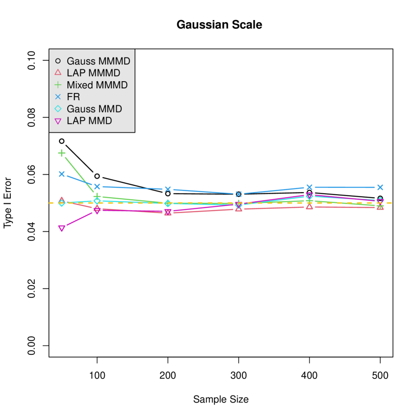
(a)

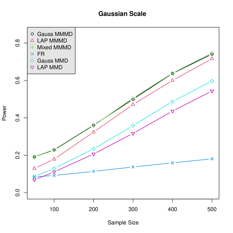
(b)

Figure 1. (a) Empirical type-I errors and (b) powers of the different tests in dimension $d=2$ with varying sample size.

7.2. Dependence on Dimension

In this section we study the performance of the different tests as dimension varies in the following 4 settings. We fix sample sizes $m=n=100$, vary dimension over $d\in\{5,10,25,50,75,100,150\}$, and compute the empirical power by averaging over 500 iterations.

1. Gaussian location-scale: Here, we consider $P=\mathcal{N}_{d}(\bm{0},\bm{\Sigma}_{0})\text{ and }Q=\mathcal{N}_{d}\left(0.1\bm{1},1.15\bm{\Sigma}_{0}\right)$, where $\bm{\Sigma}_{0}=((0.5^{|i-j|}))_{1\leq i,j\leq d}$ (see Figure 2(a)).

2. $t$-distribution scale: Here, we consider $P=t_{10}(\bm{0},\bm{\Sigma}_{0})\text{ and }Q=t_{10}\left(\bm{0},1.22\bm{\Sigma}_{0}\right)$, where $t_{10}$ is the $t$-distribution with 10 degrees of freedom and $\bm{\Sigma}_{0}$ is as above (see Figure 2(b)).

3. Gaussian and $t$-distribution mixture: Here, we consider

   $$P=\tfrac{1}{2}\mathcal{N}_{d}(\bm{0},\bm{\Sigma}_{0})+\tfrac{1}{2}t_{10}(\bm{0},\bm{\Sigma}_{0})\text{ and }Q=\tfrac{1}{2}\mathcal{N}_{d}(\bm{0},1.22\bm{\Sigma}_{0})+\tfrac{1}{2}t_{10}(\bm{0},1.22\bm{\Sigma}_{0}),$$

   where $\bm{\Sigma}_{0}$ is as above (see Figure 3(a)).

4. Gaussian and Laplace mixture: Here, we consider

   $$P=\tfrac{1}{2}\mathcal{N}_{d}(\bm{0},\bm{\Sigma}_{1})+\tfrac{1}{2}t_{10}(\bm{0},\bm{\Sigma}_{1})\text{ and }Q=\tfrac{1}{2}\mathcal{N}_{d}(\bm{0},1.3\bm{\Sigma}_{1})+\tfrac{1}{2}t_{10}(\bm{0},1.3\bm{\Sigma}_{1}),$$

   where $\bm{\Sigma}_{1}=((0.7^{|i-j|}))_{1\leq i,j\leq d}$ (see Figure 3(b)).

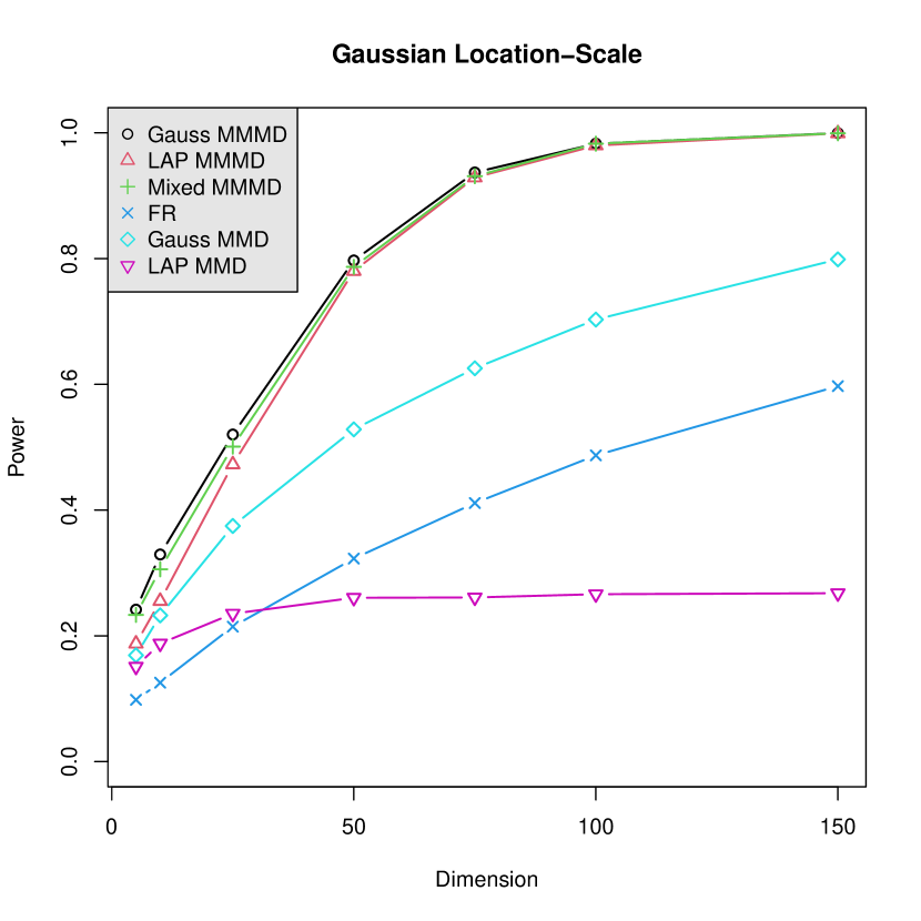
(a)

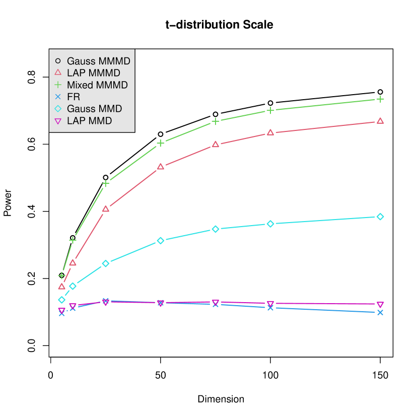
(b)

Figure 2. Empirical powers of the different tests as the dimension varies in (a) setting (S1) and (b) setting (S2).

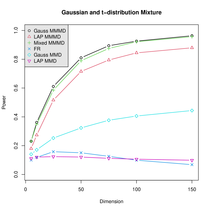
(a)

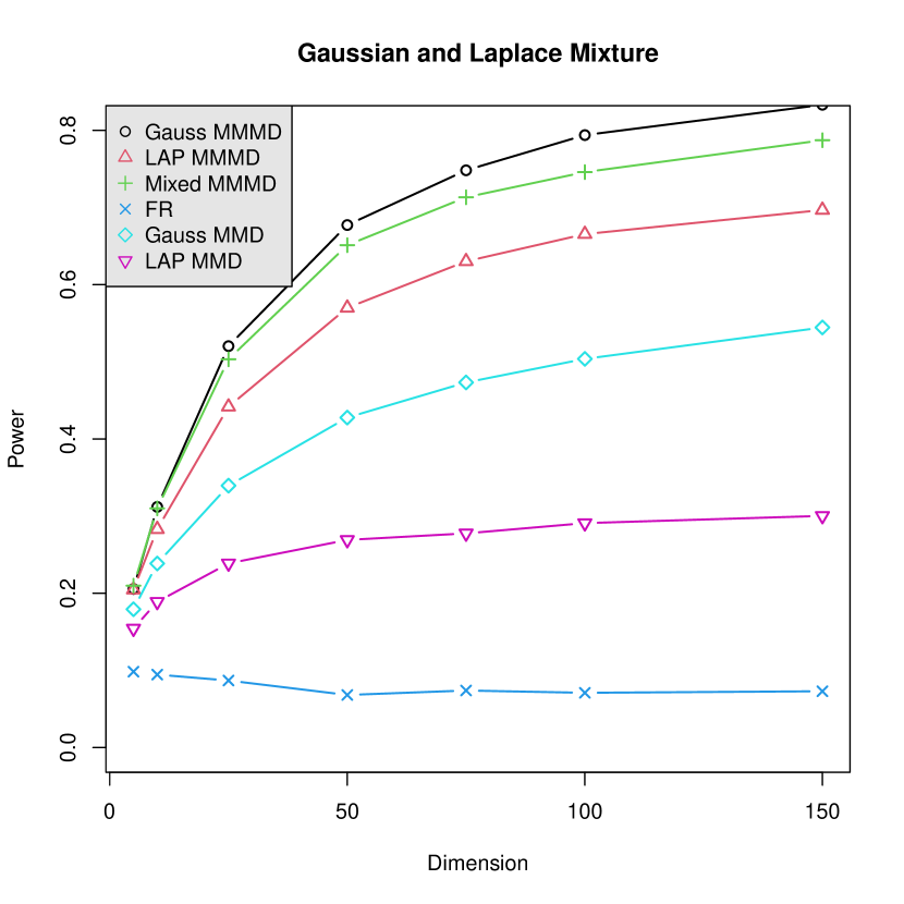
(b)

Figure 3. Empirical powers of the different tests as the dimension varies in (a) setting (S3) and (b) setting (S4).

The plots show that the multiple kernel MMMD tests have significantly more power than the single kernel MMD tests and the FR test in all the 4 settings. Overall the Gauss MMMD and the Mixed MMMD tests perform the best, closely followed by the Lap MMMD. This also shows the advantage of aggregating kernels across a range of dimensions, from low dimensions to dimensions that are comparable and even larger than the sample size.

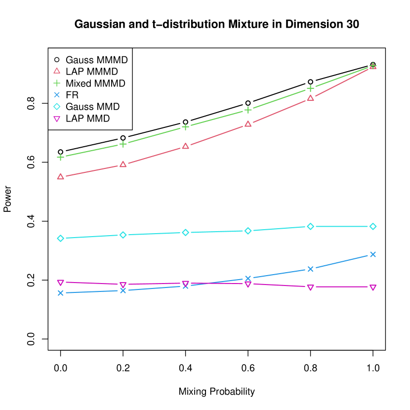
(a)

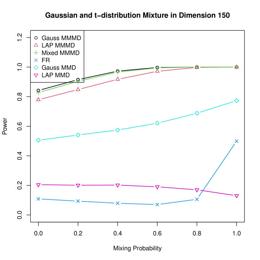
(b)

Figure 4. Empirical powers of the different tests for mixture alternatives as a function of the mixing proportion for dimension (a) $d=30$ and (b) $d=150$.

7.3. Mixture Alternatives

In this section we evaluate the performance of the tests for mixture alternatives by varying the mixing proportion. To this end, suppose $\bm{\Sigma}_{0}=((0.5^{|i-j|}))_{1\leq i,j\leq d}$ and consider

$$P=\varepsilon\mathcal{N}_{d}(\bm{0},\bm{\Sigma}_{0})+(1-\varepsilon)t_{10}(\bm{0},\bm{\Sigma}_{0})\text{ and }Q=\varepsilon\mathcal{N}_{d}(\bm{0},1.25\bm{\Sigma}_{0})+(1-\varepsilon)t_{10}(\bm{0},1.25\bm{\Sigma}_{0}).$$

Figure 4 shows the empirical power (averaged over 500 iterations) of the different tests as $\varepsilon$ varies over $[0,1]$, with sample sizes $m=n=100$ and dimension $d=30$ (Figure 4(a)) and $d=150$ (Figure 4 (b)). In both cases, the MMMD tests outperform the single kernel tests and the FR test, again illustrating the versatility of the aggregated tests.

7.4. Local Alternatives

Recall that in Section 5 we derived the asymptotic local power of the MMMD statistic. Here we validate this in the following simulation setting:

$$P=\mathcal{N}_{d}(\bm{0},\bm{I}_{d})\text{ and }Q=\mathcal{N}_{d}\left(\bm{0},(1+\tfrac{h}{\sqrt{N}})\bm{I}_{d}\right),$$ (7.4)

where $N=m+n$. Figure 5(a) shows the empirical power (averaged over 500 iterations) of the different tests, for dimension $d=20$, sample sizes $m=n=100$, as the signal strength varies over [0,3]. The plots show that the MMMD methods have significantly better local power than the other tests, illustrating the attractive efficiency property of our aggregation method.

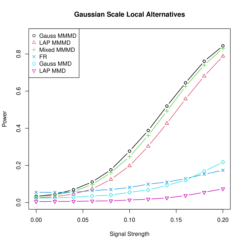
(a)

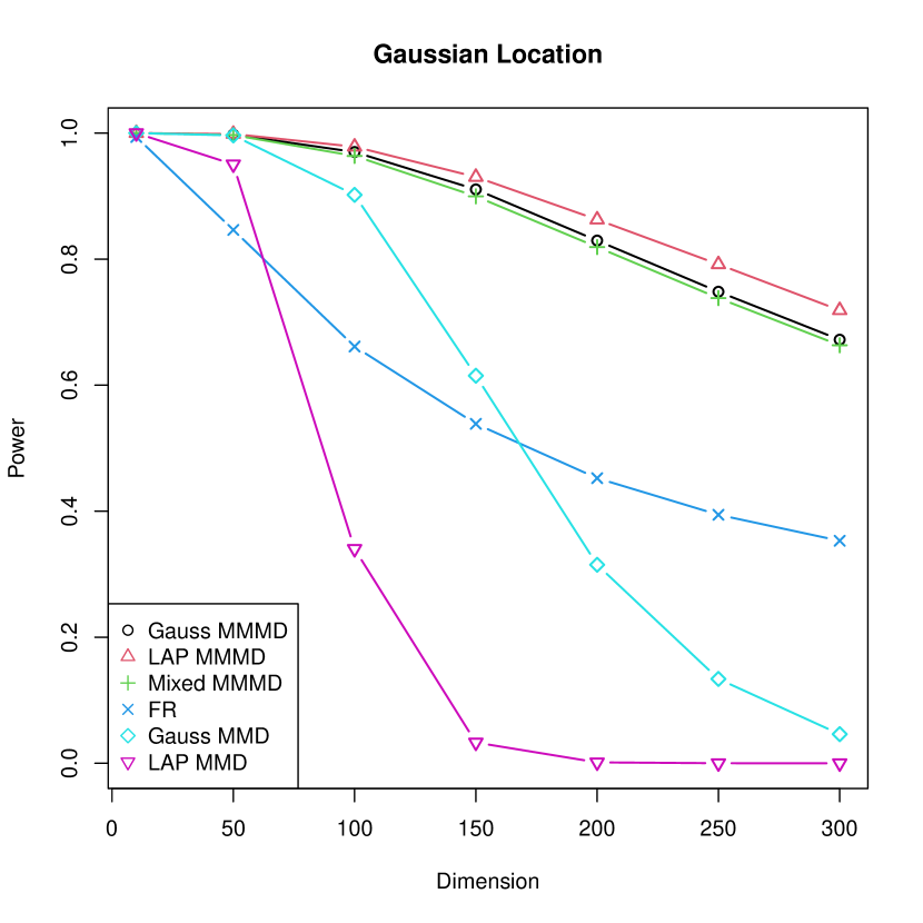
(b)

Figure 5. Empirical powers of the different tests for (a) local alternatives as in (7.4) and (b) high-dimensional alternatives as in (7.5).

7.5. High-Dimensional Alternatives

To fairly evaluate the performance of kernel tests in high-dimensions we consider, as suggested by Ramdas et al. [48], pairs of distributions for which the Kullback-Leibler (KL) divergence remain constant, as the dimension increases. Specifically, we consider following

$$P=\mathcal{N}_{d}\left(\bm{0},\bm{I}_{d}\right)\text{ and }Q=\mathcal{N}_{d}\left((1.25/\sqrt{d})\bm{1},\bm{I}_{d}\right).$$ (7.5)

It is easy to check that the KL divergence between $P$ and $Q$ is $\frac{1.25^{2}}{2}$, which does not change with $d$. In this case for the Gauss MMMD/LAP MMMD tests we use 5 different Gaussian/Laplace kernels with respective bandwidths $\bm{\sigma}=(\sigma_{1},\sigma_{2},\sigma_{3},\sigma_{4},\sigma_{5})=(\tfrac{1}{2\sqrt{2}},\tfrac{1}{2},\frac{1}{\sqrt{2}},1,\sqrt{2})\lambda_{\text{med}}$. Also, for the Mixed MMMD test is implemented with 4 Gaussian kernels and 4 Laplace kernels with same set of bandwidths: $\bm{\sigma}=(\sigma_{1},\sigma_{2},\sigma_{3},\sigma_{4})=(\frac{1}{2},\frac{1}{\sqrt{2}},1,\sqrt{2})\lambda_{\text{med}}$. Figure 5(b) shows the empirical powers (averaged over 500 iterations) of the different tests as a function of dimension with sample sizes $m=n=100$. As expected, the power of all the tests decreases as dimension increases. However, for the multiple kernel tests the power decrement is much slower and overall they perform significantly better than the single kernel tests.

8. Real Data Applications

In this section we apply our method to compare images of digits in the noisy MNIST dataset. Specifically, consider two noisy versions of the MNIST dataset: (1) MNIST with additive Gaussian noise (Section 8.1), and (2) MNIST with reduced contrast and additive noise, where, in addition to the Gaussian noise the contrast of the images is reduced (Section 8.2). As in the previous section, we implement the single kernel Gauss MMD and LAP MMD tests with the median bandwidth, the multiple kernel Gauss MMMD, LAP MMMD, and Mixed MMMD tests with bandwidths as in (7.1), (7.2), (7.3), respectively, and the FR test using the R package gTests.

8.1. MNIST with Additive Gaussian Noise

In this section we illustrate the performance of the proposed test in detecting different sets of digits when i.i.d. Gaussian noise with standard deviation $\sigma$ is added to each pixel. Figure 6 shows how such noisy data looks for (a) $\sigma=0$ (which is the clean data with no noise), (b) $\sigma=0.6$ and (c) $\sigma=1$.

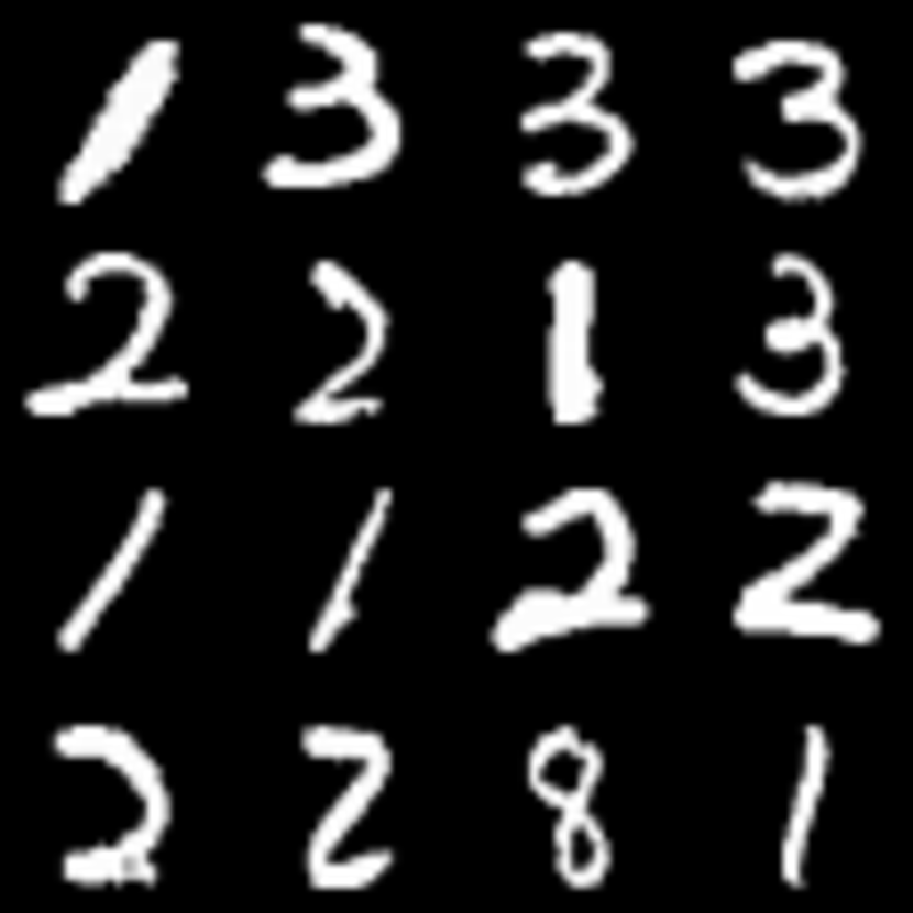
(a) Clean data

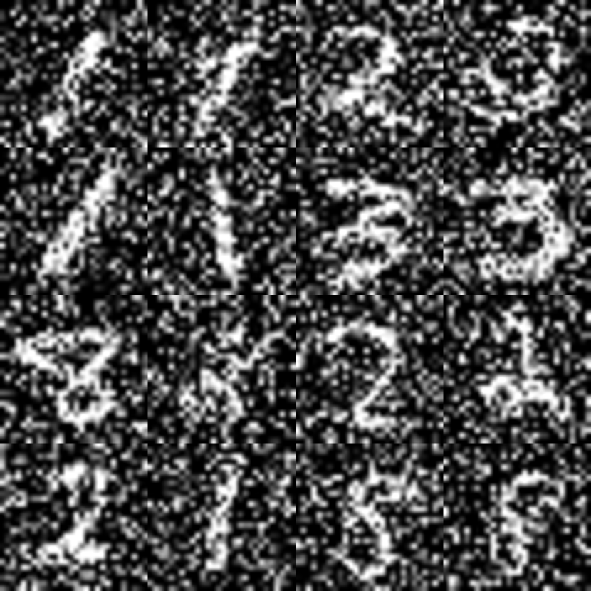
(b) Noisy data with $\sigma=0.6$

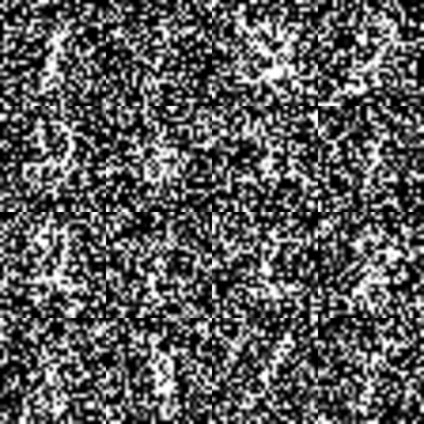
(c) Noisy data with $\sigma=1$

Figure 6. MNIST data with additive Gaussian noise.

To evaluate the proposed method we consider the following sets of digits:

$$P=\{1,2,3\}\text{ and }Q=\{1,2,8\},$$

and vary the standard error $\sigma\in(0,0.2,0.4,0.6,0.8,1)$. For each $\sigma$ we draw $100$ samples with replacements from the two sets and check if the tests successfully reject $H_{0}$ at level $\alpha=0.5$. We repeat this experiment $500$ times to estimate the power. Figure 7 shows performance of the above mentioned tests, where we plot the power over the index of pair of sets of digits. This shows that for the clean data and for small noise levels, the singe kernel Gauss MMD performs comparably with the MMMD tests. However, for larger noise levels the MMMD tests perform much than the single kernel tests. The FR test also perform well in this case across the range of the noise level.

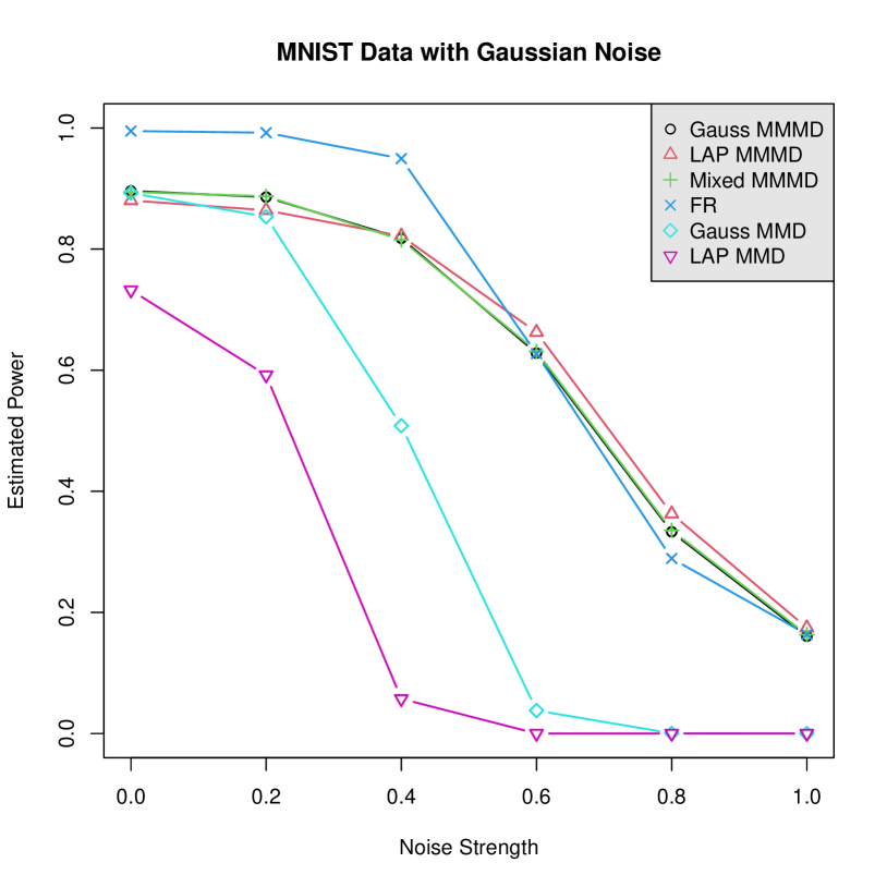
Figure 7. Estimated powers of the tests on noisy MNIST dataset with increasing noise strength.

8.2. MNIST with reduced contrast and additive Gaussian noise

In this section we illustrate the performance of the different tests on the noisy version of the MNIST dataset considered in [6]. (The dataset is publicly available at https://csc.lsu.edu/~saikat/n-mnist/) Here, in addition to additive Gaussian noise the contrast of the images is also reduced. Specifically, the contrast range is scaled down to half and an additive Gaussian noise is introduced with signal-to-noise ratio of 12. This emulates background clutter along with significant change in lighting conditions (see Figure 8 for an example of such a noisy image).

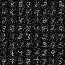
(a)

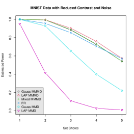
(b)

Figure 8. (a) MNIST dataset with reduced contrast and additive white gaussian noise and (b) estimated power.

We evaluate the performance of the different test for the following 5 pairs of sets of digits:

1. $P=\{2,4,8,9\}$ and $Q=\{3,4,7,9\}$,

2. $P=\{1,2,4,8,9\}$ and $Q=\{1,3,4,7,9\}$,

3. $P=\{0,1,2,4,8,9\}$ and $Q=\{0,1,3,4,7,9\}$,

4. $P=\{0,1,2,4,5,8,9\}$ and $Q=\{0,1,3,4,5,7,9\}$,

5. $P=\{0,1,2,4,5,6,8,9\}$ and $Q=\{0,1,3,4,5,6,7,9\}$.

For each of the 5 cases above, we draw $150$ samples with replacements from the two sets and check if the tests successfully reject $H_{0}$ at level $\alpha=0.5$. We repeat this experiment $500$ times to estimate the power. Figure 8 shows the power of the different for the above 5 sets. In this case, the multiple kernel tests and the FR test overall has the highest power across the 5 sets, followed by the Gauss MMD and the Lap MMD.

9. Broader Scope

The idea of using multiple kernels/bandwidths has recently emerged as a popular alternative to selecting a single bandwidth, for developing adaptive kernel two-sample tests that do not require data-splitting. In this direction, Kübler et al. [37] proposed a method which does not require data splitting using the framework of post-selection inference. However, this method requires asymptotic normality of the test statistic under $H_{0}$, hence, is restricted to the linear-time MMD estimate [23, Section 6], which leads to loss in power when compared to the more commonly used quadratic-time estimate (2.6). Fromont et al. [21, 20] and, more recently, Schrab et al. [55] introduced another non-asymptotic aggregated test, hereafter referred to as MMDAgg, that is adaptive minimax (up to an iterated logarithmic term) over Sobolev balls.

Our aggregation strategy, leads to a test that can be efficiently implemented, enjoy improved empirical power over single kernel tests for a range of alternatives, and scales well in high dimensions. Moreover, instead of minimax optimality, our focus is on establishing the asymptotic properties of the aggregated test. Towards this, we derive the joint distribution of the MMD estimates (under both local and fixed alternatives) and, consequently, establish the statistical (Pitman) efficiency of the proposed test. In fact, our theoretical results apply to general aggregation schemes using which we can obtain the asymptotic efficiency of the aforementioned MMDAgg test (see Section 9.1). Numerical results comparing the empirical power of the MMMD test with the MMDAgg test are reported in Section 9.2. Interestingly, MMMD has better power than MMDAgg for a range of alternatives, which include perturbed uniform distributions in the Sobolev class, as well as natural mixture and local alternatives. This showcases both the practical relevance of the Mahalanobis aggregation strategy and the broader scope of our asymptotic results.

9.1. Local Asymptotic Power of the MMDAgg Test

In this section, we propose an asymptotic implementation of the MMDAgg test and sketch a heuristic argument that derives its limiting local power in the contamination model (5.2). The argument can be made rigorous by using tools from empirical process theory, however, since the purpose of this section is more illustrative than technical, we have not pursued this direction.

To describe the asymptotic version of the MMDAgg test suppose $\mathcal{K}=\{{\mathsf{K}}_{1},{\mathsf{K}}_{2},\ldots,{\mathsf{K}}_{r}\}$ is a finite collection of kernels and $\mathcal{W}:=\{w_{1},w_{2},\ldots,w_{r}\}$ is an associated collection of positive weights such that $\sum_{s=1}^{r}w_{s}\leq 1$. Moreover, for $\alpha\in(0,1)$ and $1\leq s\leq r$, let $\hat{q}_{1-\alpha,s,m}$ be the $\alpha$-th quantile of the distribution

$$\mathscr{E}({\mathsf{K}}_{s},\mathscr{X}_{m}):=\bm{Z}_{m}^{\top}{\hat{\bm{{\mathsf{K}}}}^{\circ}}_{s}\bm{Z}_{m}-\frac{1}{\hat{\rho}(1-\hat{\rho})}\operatorname{Tr}[{\hat{\bm{{\mathsf{K}}}}^{\circ}}_{s}].$$

where ${\hat{\bm{{\mathsf{K}}}}^{\circ}}_{s}$ is as defined in (4.1), for $1\leq a\leq r$, and $\bm{Z}_{m}\sim\mathcal{N}_{m}(\bm{0},\frac{1}{\hat{\rho}(1-\hat{\rho})}\bm{I})$ is independent of $\mathscr{X}_{m}$. The idea of the MMDAgg test is to reject $H_{0}$ if any one of the individual (single-kernel) test based on the kernels in $\mathcal{K}$ rejects $H_{0}$ for a specially chosen cut-off (see [55, Section 3.5] for details). Here, we consider an alternative implementation of MMDAgg test based on the Gaussian multiplier bootstrap discussed in Section 4. To this end, define

$$u^{*}_{\alpha,m}:=\mathrm{arg}\max\left\{u\in(0,L):\mathbb{P}\left(\max_{1\leq s\leq r}\left\{\mathscr{E}({\mathsf{K}}_{s},\mathscr{X}_{m})-\hat{q}_{1-uw_{s},s,m}\right\}>0|\mathscr{X}_{m}\right)\leq\alpha\right\},$$

where $L:=\min_{1\leq s\leq r}w_{s}^{-1}$. (Note that the probability in the RHS above is over the randomness of $\bm{Z}_{m}$ (conditional on $\mathscr{X}_{m}$), hence, $u^{*}_{\alpha,m}$ can be computed from the data by a grid search over $u\in(0,L)$.) The MMDAgg test would then reject $H_{0}$ if

$$\phi_{m,n,\alpha}^{\mathrm{MMDAgg}}:=\bm{1}\left\{\max_{1\leq s\leq r}\left\{\mathrm{MMD}^{2}\left[{\mathsf{K}}_{s},\mathscr{X}_{m},\mathscr{Y}_{n}\right]-\hat{q}_{1-w_{s}u^{*}_{\alpha},s,m}\right\}>0\right\}.$$ (9.1)

To describe the asymptotic properties of this test, let $q_{\alpha,s}$ be the $\alpha$-th quantile of the distribution $\frac{1}{\rho(1-\rho)}I_{2}({\mathsf{K}}^{\circ}_{s})$, for $1\leq s\leq r$. Then for each fixed $u\in(0,L)$, by Theorem 3.1, Slutsky’s theorem, and the continuous mapping theorem, as $m\rightarrow\infty$,

$$\max_{1\leq s\leq r}\left\{\mathscr{E}({\mathsf{K}}_{s},\mathscr{X}_{m})-\hat{q}_{1-uw_{s},s,m}\right\}\stackrel{{\scriptstyle D}}{{\to}}\max_{1\leq s\leq r}\left\{\frac{1}{\rho(1-\rho)}I_{2}({\mathsf{K}}^{\circ}_{s})-q_{1-uw_{s},s}\right\}.$$

since $\hat{q}_{1-uw_{s},s,m}|\mathscr{X}_{m}\stackrel{{\scriptstyle a.s.}}{{\rightarrow}}q_{1-uw_{s},s}$. Therefore, for each fixed $u\in(0,L)$, as $m\rightarrow\infty$,

$$\mathbb{P}\left(\max_{1\leq s\leq r}\left\{\mathscr{E}({\mathsf{K}}_{s},\mathscr{X}_{m})-\hat{q}_{1-uw_{s},s,m}\right\}>0|\mathscr{X}_{m}\right)\rightarrow\mathbb{P}\left(\max_{1\leq s\leq r}\left\{\frac{1}{\rho(1-\rho)}I_{2}({\mathsf{K}}^{\circ}_{s})-q_{1-uw_{s},s}\right\}>0\right).$$

Now, since the convergence of the quantiles is uniform, we expect the following to hold as $m\rightarrow\infty$:

$$u^{*}_{\alpha,m}\stackrel{{\scriptstyle a.s.}}{{\rightarrow}}u^{*}_{\alpha}\quad\text{ and }\quad\hat{q}_{1-w_{s}u^{*}_{\alpha,m},s,m}|\mathscr{X}_{m}\stackrel{{\scriptstyle a.s.}}{{\rightarrow}}q_{1-w_{s}u^{*}_{\alpha},s},$$

where

$$u^{*}_{\alpha}:=\mathrm{arg}\max\left\{u\in(0,L):\mathbb{P}\left(\max_{1\leq s\leq r}\left\{\frac{1}{\rho(1-\rho)}I_{2}({\mathsf{K}}^{\circ}_{s})-q_{1-uw_{s},s}\right\}>0\right)\leq\alpha\right\}.$$

Hence, under $H_{1}$ as in (5.2), by Theorem 5.1, Slutsky’s theorem, and the continuous mapping theorem,

$$\max_{1\leq s\leq r}\left\{\mathrm{MMD}^{2}\left[{\mathsf{K}}_{s},\mathscr{X}_{m},\mathscr{Y}_{n}\right]-\hat{q}_{1-w_{s}u^{*}_{\alpha},s,m}\right\}\stackrel{{\scriptstyle D}}{{\to}}\max_{1\leq s\leq r}\left\{G_{{\mathsf{K}}_{s},h}-q_{1-w_{s}u^{*}_{\alpha},s}\right\},$$

where

$$G_{{\mathsf{K}}_{s},h}:=\gamma I_{2}({\mathsf{K}}^{\circ}_{s})+2h\sqrt{\gamma}I_{1}\left({\mathsf{K}}^{\circ}_{s}\left[\frac{g}{f_{P}}\right]\right)+h^{2}\mu_{s},$$

and $\mu_{s}$ is as defined in (5.8). Therefore, the limiting power of the test (9.1) is given by

$$\lim_{m,n\rightarrow\infty}\mathbb{E}_{H_{1}}[\phi_{m,n,\alpha}^{\mathrm{MMDAgg}}] =\mathbb{P}\left(\max_{1\leq s\leq r}\left\{G_{{\mathsf{K}}_{s},h}-q_{1-w_{s}u^{*}_{\alpha},s}\right\}>0\right)$$

$$=1-\mathbb{P}\left(G_{{\mathsf{K}}_{s},h}\leq q_{1-w_{s}u^{*}_{\alpha},s},\text{ for all }1\leq s\leq r\right)$$

$$=1-\bm{F}_{\mathcal{K},h}(q_{1-w_{1}u^{*}_{\alpha},1},\ldots,q_{1-w_{r}u^{*}_{\alpha},r}),$$

where $\bm{F}_{\mathcal{K},h}$ is the cumulative distribution function of the vector $(G_{{\mathsf{K}}_{1},h},G_{{\mathsf{K}}_{2},h},\ldots,G_{{\mathsf{K}}_{r},h})^{\top}$.

9.2. Empirical Comparison

In this section we compare the MMMD test with the MMDAgg test as implemented in [55].

9.2.1. Perturbed $1$-dimensional Uniform Distribution

First we consider a perturbed version of uniform distribution on $[0,1]$ as considered [55]. The perturbed density at $x\in\mathbb{R}$ is given by:

$$f_{\bm{\theta}}(x)=\bm{1}\left\{x\in[0,1]\right\}+\frac{c_{1}}{P}\sum_{v\in\{1,2,\ldots,P\}}\theta_{v}G\left(Px-v\right)$$

where $c_{1}=2.7$, $\bm{\theta}=(\theta_{1},\theta_{2},\cdots,\theta_{P})\in\{-1,1\}^{P}$, $P$ is the number of perturbations, and

$$G(t):=\exp\left(-\dfrac{1}{1-(4t+3)^{2}}\right)\bm{1}\left\{t\in(-1,-\tfrac{1}{2})\right\}-\exp\left(-\dfrac{1}{1-(4t+1)^{2}}\right)\bm{1}\left\{t\in(-\tfrac{1}{2},0)\right\}.$$

It is known that for $P$ large enough the difference between the uniform density and the perturbed uniform density lies in the Sobolev ball [40]. Figure 9(a) shows the empirical powers of the MMDAgg test with Gaussian and Laplace kernels, with bandwidths chosen according to the increasing weight strategy as in [55]; the empirical powers of the Gauss MMMD, LAP MMMD, and Mixed MMMD with bandwidth chosen as in (7.1), (7.2) and (7.3), respectively; and the empirical power of the FR test. The sample sizes are set to $m=n=500$, the perturbations range over $P=1,2,3,4,5,6$, and the power is computed over 500 repetitions, with a new value of $\bm{\theta}\in\{-1,1\}^{P}$ sampled uniformly in each iteration. The plot shows that the MMMD tests have better finite-sample power than the MMAgg tests, particularly for larger perturbations.

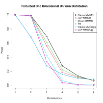
(a)

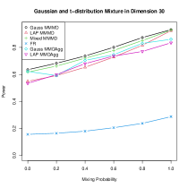
(b)

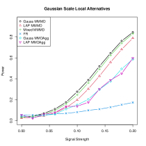
(c)

Figure 9. Empirical powers of the MMMD and MMDAgg tests for (a) the perturbed uniform distribution, (b) mixture alternatives, and (c) local alternatives.

9.2.2. Mixture and Local Alternatives

Next, we compare the empirical power (by repeating the experiment 500 times) of the MMMD tests with the MMDAgg tests (based on Gaussian and Laplace kernels) for the mixtures alternative in $d=30$ as in Section 7.3 and the local alternative in $d=20$ as in Section 7.4. For the MMMD tests we use bandwidths as in (7.1), (7.2), and (7.3), while for the MMDAgg tests we consider the increasing weight strategy with collection of bandwidths $\Lambda(-2,2)$ as defined in [55, Section 5.3]. For the mixture alternative the MMMD tests perform slightly better than the MMDAgg tests (see Figure 9(b)), while for the local alternative the MMMD tests show significant improvement over the MMDAgg tests (see Figure 9(c)).

Appendix A Proof of Theorem 3.1 and Corollary 3.1

To begin with note that the definition of $\mathrm{MMD}^{2}$ in (2.5) can be extended to any measurable and symmetric function $\mathsf{H}\in L^{2}(\mathcal{X}^{2},P^{2})$ (not necessarily positive definite) in a natural way as follows:

$$\mathrm{MMD}^{2}\left[\mathsf{H},\mathscr{X}_{m},\mathscr{Y}_{n}\right]=\mathcal{W}_{\mathscr{X}_{m}}+\mathcal{W}_{\mathscr{Y}_{n}}-2\mathcal{B}_{\mathscr{X}_{m},\mathscr{Y}_{n}},$$ (A.1)

where $\mathcal{W}_{\mathscr{X}_{m}}$, $\mathcal{W}_{\mathscr{Y}_{n}}$, and $\mathcal{B}_{\mathscr{X}_{m},\mathscr{Y}_{n}}$ are as defined in (2.6) and (2.7), respectively, with $\sf K$ replaced by $\mathsf{H}$. The main ingredient in the proof of Theorem 3.1 is the following result:

Proposition A.1 ([23, Theorem 5]).

For any measurable and symmetric function $\mathsf{H}\in L^{2}(\mathcal{X}^{2},P^{2})$, in the asymptotic regime (2.8),

$$(m+n)\mathrm{MMD}^{2}\left[\mathsf{H},\mathscr{X}_{m},\mathscr{Y}_{n}\right]:=\frac{1}{\rho(1-\rho)}\sum_{s=1}^{\infty}\lambda_{s}\left(Z_{s}^{2}-1\right),$$ (A.2)

where $\{Z_{s}:s\geq 1\}$ are i.i.d. $\mathcal{N}(0,1)$ and $\{\lambda_{s}\}_{s\geq 1}$ are the eigenvalues (with repetitions) of the Hilbert-Schimdt operator $\mathcal{H}_{\mathsf{H}^{\circ}}$ defined as:

$$\mathcal{H}_{\mathsf{H}^{\circ}}[f(x)]=\int_{\mathcal{X}}\mathsf{H}^{\circ}(x,y)f(y)\mathrm{d}P(y),$$ (A.3)

with $\mathsf{H}^{\circ}(x,y):=\mathsf{H}(x,y)-\mathbb{E}_{X\sim P}\mathsf{H}(X,y)-\mathbb{E}_{X^{\prime}\sim P}\mathsf{H}(x,X^{\prime})+\mathbb{E}_{X,X^{\prime}\sim P}\mathsf{H}(X,X^{\prime})$. Moreover, the characteristic function of $Z(\mathsf{H})$ at $t\in\mathbb{R}$ is given by:

$$\Phi_{Z(\mathsf{H})}(t):=\mathbb{E}\left[e^{\iota tZ(\mathsf{H})}\right]=\prod_{s=1}^{\infty}\frac{e^{-\frac{\iota\lambda_{s}t}{\rho(1-\rho)}}}{\sqrt{1-\frac{2\iota\lambda_{s}t}{\rho(1-\rho)}}}.$$ (A.4)

Remark A.1.

The convergence in (A.2) is a consequence of [23, Theorem 5], while the expression of the characteristic function in (A.4) follows from [31, Proposition 6.1]. (Note that Proposition A.1 also follows from the proof of Proposition C.1 in Section C by setting $h=0$).

We now present the proof of Theorem 3.1 in Appendix A.1. The proof of Corollary 3.1 is given in Appendix A.2.

A.1. Proof of Theorem 3.1

First recall the definition of $\mathrm{MMD}^{2}[\mathcal{K},\mathscr{X}_{m},\mathscr{Y}_{n}]$ from (2.10). Note that for $\bm{\eta}=(\eta_{1},\eta_{2},\ldots,\eta_{r})^{\top}\in\mathbb{R}^{r}$,

$$\bm{\eta}^{\top}\mathrm{MMD}^{2}[\mathcal{K},\mathscr{X}_{m},\mathscr{Y}_{n}]=\sum_{a=1}^{r}\eta_{a}\mathrm{MMD}^{2}[{\mathsf{K}}_{a},\mathscr{X}_{m},\mathscr{Y}_{n}] =\mathrm{MMD}^{2}[\mathsf{H}_{\bm{\eta}},\mathscr{X}_{m},\mathscr{Y}_{n}],$$ (A.5)

where $\mathsf{H}_{\bm{\eta}}:=\sum_{a=1}^{r}\eta_{a}{\mathsf{K}}_{a}$. Clearly, $\mathsf{H}_{\bm{\eta}}$ is a measurable and symmetric function and $\mathsf{H}_{\bm{\eta}}\in L^{2}\left(\mathcal{X},P^{2}\right)$ (by Assumption 2.1). Then by Proposition A.1,

$$Z_{m,n}(\mathsf{H}_{\bm{\eta}}):=(m+n)\mathrm{MMD}^{2}\left[\mathsf{H}_{\bm{\eta}},\mathscr{X}_{m},\mathscr{Y}_{n}\right]\stackrel{{\scriptstyle D}}{{\to}}Z(\mathsf{H}_{\bm{\eta}})=\frac{1}{\rho(1-\rho)}\sum_{\lambda\in\Lambda(\bm{\eta})}\lambda\left(Z_{\lambda}^{2}-1\right).$$ (A.6)

where $\{Z_{\lambda}\}_{\lambda\in\Lambda(\bm{\eta})}$ are i.i.d. $\mathcal{N}(0,1)$ and $\Lambda(\bm{\eta})$ are the eigenvalues (with repetitions) of the Hilbert-Schimdt operator:

$$\mathcal{H}_{\mathsf{H}_{\bm{\eta}}^{\circ}}[f(x)]=\int\mathsf{H}_{\bm{\eta}}^{\circ}(x,y)f(y)\mathrm{d}P(y),$$ (A.7)

with

$$\mathsf{H}_{\bm{\eta}}^{\circ}(x,y) :=\mathsf{H}_{\bm{\eta}}(x,y)-\mathbb{E}_{X\sim P}\mathsf{H}_{\bm{\eta}}(X,y)-\mathbb{E}_{X^{\prime}\sim P}\mathsf{H}_{\bm{\eta}}(x,X^{\prime})+\mathbb{E}_{X,X^{\prime}\sim P}\mathsf{H}_{\bm{\eta}}(X,X^{\prime})$$

$$=\sum_{a=1}^{r}\eta_{a}{\mathsf{K}}^{\circ}_{a}(x,y),$$ (A.8)

Hence, the operator $\mathcal{H}_{\mathsf{H}_{\bm{\eta}}^{\circ}}$ in (A.7) is same as the operator $\mathcal{H}_{\mathcal{K},\bm{\eta}}$ defined in (3.6). Then Proposition A.1, (A.6), and (A.1) implies,

$$\mathbb{E}\left[e^{\iota Z_{m,n}(\mathsf{H}_{\bm{\eta}})}\right]\rightarrow\mathbb{E}\left[e^{\iota Z(\mathsf{H}_{\bm{\eta}})}\right]=\prod_{\lambda\in\Lambda(\bm{\eta})}\frac{e^{-\frac{\iota\lambda}{\rho(1-\rho)}}}{\sqrt{1-\frac{2\iota\lambda}{\rho(1-\rho)}}}=\Phi(\bm{\eta}),$$ (A.9)

where $\Phi(\bm{\eta})$ is as defined in (3.5). Since $\bm{\eta}\in\mathbb{R}^{r}$ was chosen arbitrarily and $\Phi(\bm{\eta})$ is continuous at $\bm{\eta}=\bm{0}\in\mathbb{R}^{r}$ (by Lemma F.1), Levy’s continuity theorem [17, Theorem 3.3.17] implies that there exists a random variable $Z_{\mathcal{K}}$ with characteristic function $\Phi(\bm{\eta})$ such that,

$$\mathrm{MMD}^{2}[\mathcal{K},\mathscr{X}_{m},\mathscr{Y}_{n}]\stackrel{{\scriptstyle D}}{{\to}}Z_{\mathcal{K}}.$$ (A.10)

We now show that the limit $Z_{\mathcal{K}}$ in (A.10) can be expressed as $G_{\mathcal{K}}$ in (3.4). Towards this, note that by the linearity of multiple stochastic integrals,

$$\mathbb{E}\left[e^{\iota\bm{\eta}^{\top}G_{\mathcal{K}}}\right]=\mathbb{E}\left[e^{\frac{\iota}{\rho(1-\rho)}\sum_{a=1}^{r}\eta_{a}I_{2}(\sf K_{a}^{\circ})}\right]=\mathbb{E}\left[e^{\frac{\iota}{\rho(1-\rho)}I_{2}(\sum_{a=1}^{r}\eta_{a}\sf K_{a}^{\circ})}\right]=\mathbb{E}\left[e^{\frac{\iota}{\rho(1-\rho)}I_{2}(\mathsf{H}_{\bm{\eta}}^{\circ})}\right],$$ (A.11)

where the last step uses (A.1). Then by [31, Theorem 6.1], $I_{2}(\mathsf{H}_{\bm{\eta}}^{\circ})$ has characteristic function:

$$\Phi_{\mathsf{H}_{\bm{\eta}}^{\circ}}(s):=\mathbb{E}\left[e^{\iota sI_{2}(\mathsf{H}_{\bm{\eta}}^{\circ})}\right]=\prod_{\lambda\in\Lambda(\bm{\eta})}\dfrac{e^{-\iota\lambda s}}{\sqrt{1-2\iota\lambda s}}$$ (A.12)

where $\Lambda(\bm{\eta})$ is the set of eigenvalues (with repetition) of the bilinear form $\mathcal{B}_{\mathsf{H}_{\bm{\eta}}^{\circ}}:L^{2}(\mathcal{X})\times L^{2}(\mathcal{X})\rightarrow\mathbb{R}$:

$$\mathcal{B}_{\mathsf{H}_{\bm{\eta}}^{\circ}}(f_{P},f_{2}):=\frac{1}{2}\mathbb{E}\left[I_{2}(\mathsf{H}_{\bm{\eta}}^{\circ})I_{1}(f_{1})I_{1}(f_{2})\right],$$

for any $f_{1},f_{2}\in L^{2}(\mathcal{X},P)$. Now, using the multiplication formula for stochastic integrals (cf. [31, Theorem 7.33]) gives,

$$\frac{1}{2}\mathbb{E}\left[I_{2}(\mathsf{H}_{\bm{\eta}}^{\circ})I_{1}(f_{1})I_{1}(f_{2})\right] =\frac{1}{2}\int_{\mathcal{X}^{2}}\left[\mathsf{H}_{\bm{\eta}}^{\circ}(x,y)f_{1}(x)f_{2}(y)+\mathsf{H}_{\bm{\eta}}^{\circ}(x,y)f_{1}(y)f_{2}(x)\right]\mathrm{d}P(x)\mathrm{d}P(y)$$

$$=\int_{\mathcal{X}^{2}}\mathsf{H}_{\bm{\eta}}^{\circ}(x,y)f_{1}(x)f_{2}(y)\mathrm{d}P(x)\mathrm{d}P(y),$$

where the last equality follows by symmetry of the function $\mathsf{H}_{\bm{\eta}}^{\circ}$. This shows that the bilinear form $\mathcal{B}_{\mathsf{H}_{\bm{\eta}}^{\circ}}$ has the same set of eigenvalues (with repetitions) as that of the operator $\mathcal{H}_{\mathsf{H}_{\bm{\eta}}^{\circ}}$ defined in (A.1). Hence, combining (A.11) and (A.12) it follows that,

$$\mathbb{E}\left[e^{\iota\bm{\eta}^{\top}G_{\mathcal{K}}}\right]=\Phi_{\mathsf{H}_{\bm{\eta}}^{\circ}}\left(\frac{1}{\rho(1-\rho)}\right)=\prod_{\lambda\in\Lambda(\bm{\eta})}\frac{e^{-\frac{\iota\lambda}{\rho(1-\rho)}}}{\sqrt{1-\frac{2\iota\lambda}{\rho(1-\rho)}}},$$ (A.13)

where $\Lambda(\bm{\eta})$ is the set of eigenvalues (with repetitions) of the operator $\mathcal{H}_{\mathsf{H}_{\eta}^{\circ}}$, which the same as the operator $\mathcal{H}_{\mathcal{K},\bm{\eta}}$ (by (3.6)). Note that the RHS of (A.13) equals the function $\Phi(\bm{\eta})$ defined in (3.5), which implies that $Z_{\mathcal{K}}$ in (A.10) has the same distribution as $G_{\mathcal{K}}$ in (3.4). This completes the proof of Theorem 3.1. $\Box$

A.2. Proof of Corollary 3.1

Recall the definition of the centered kernel ${\mathsf{K}}_{a}^{\circ}$ from (2.13). Then it is easy to see that

$$\mathrm{MMD}^{2}\left[{\mathsf{K}}_{a},\mathscr{X}_{m},\mathscr{Y}_{n}\right]=\mathrm{MMD}^{2}\left[{\mathsf{K}}_{a}^{\circ},\mathscr{X}_{m},\mathscr{Y}_{n}\right].$$

Observe that $\mathbb{E}\left[{\mathsf{K}}_{a}^{\circ}(X_{1},X_{2})\middle|X_{1}\right]=0$ and hence $\operatorname{Cov}\left({\mathsf{K}}_{a}^{\circ}(X_{1},X_{2}){\mathsf{K}}_{b}^{\circ}(X_{1},X_{3})\right)=0$, for $X_{1},X_{2},X_{3}$ i.i.d. from the distribution $P$. Then by a direct computation it follows that, for $1\leq a,b\leq r$,

$$\sigma_{ab}=\frac{2}{\rho^{2}(1-\rho)^{2}}\mathbb{E}_{X,X^{\prime}\sim P}\left[{\mathsf{K}}_{a}^{\circ}(X,X^{\prime}){\mathsf{K}}_{b}^{\circ}(X,X^{\prime})\right].$$ (A.14)

This proves (3.9).

Next, we prove (3.10). For all $1\leq a\leq r$, define

$$\bm{{\mathsf{K}}}^{\circ}_{a}=\left(\left({\mathsf{K}}_{a}^{\circ}(X_{i},X_{j})/m\right)\right)_{1\leq i,j\leq m}$$

where ${\mathsf{K}}_{a}^{\circ}$ is defined in Theorem 3.1. Also, recall the definition of ${\hat{\bm{{\mathsf{K}}}}^{\circ}}_{a}$, for $1\leq a\leq r$, from (4.1). Now, observe that for any $1\leq a,b\leq r$,

$$\left|\operatorname{Tr}\left[{\hat{\bm{{\mathsf{K}}}}^{\circ}}_{a}{\hat{\bm{{\mathsf{K}}}}^{\circ}}_{b}\right]-\operatorname{Tr}\left[\bm{{\mathsf{K}}}^{\circ}_{a}\bm{{\mathsf{K}}}^{\circ}_{b}\right]\right| \leq\left|\operatorname{Tr}\left[{\hat{\bm{{\mathsf{K}}}}^{\circ}}_{a}{\hat{\bm{{\mathsf{K}}}}^{\circ}}_{b}\right]-\operatorname{Tr}\left[\bm{{\mathsf{K}}}^{\circ}_{a}{\hat{\bm{{\mathsf{K}}}}^{\circ}}_{b}\right]\right|+\left|\operatorname{Tr}\left[\bm{{\mathsf{K}}}^{\circ}_{a}{\hat{\bm{{\mathsf{K}}}}^{\circ}}_{b}\right]-\operatorname{Tr}\left[\bm{{\mathsf{K}}}^{\circ}_{a}\bm{{\mathsf{K}}}^{\circ}_{b}\right]\right|$$

$$\leq\|{\hat{\bm{{\mathsf{K}}}}^{\circ}}_{a}\|\|{\hat{\bm{{\mathsf{K}}}}^{\circ}}_{a}-\bm{{\mathsf{K}}}^{\circ}_{a}\|+\|\bm{{\mathsf{K}}}^{\circ}_{a}\|\|{\hat{\bm{{\mathsf{K}}}}^{\circ}}_{b}-\bm{{\mathsf{K}}}^{\circ}_{b}\|$$ (A.15)

Since ${\mathsf{K}}_{a}^{\circ}\in L^{2}(\mathcal{X}^{2},P^{2})$, by the strong law of large number for $U$-statistics (see [57, Theorem 5.4.A])

$$\|\bm{{\mathsf{K}}}^{\circ}_{a}\|^{2}=\frac{1}{m^{2}}\sum_{1\leq i,j\leq m}{{\mathsf{K}}}^{\circ}_{a}(X_{i},X_{j})^{2}\stackrel{{\scriptstyle a.s.}}{{\rightarrow}}\mathbb{E}_{X,X^{\prime}\sim P}[{{\mathsf{K}}}^{\circ}_{a}(X,X^{\prime})].$$

Also, following the proof of Lemma B.4 we have $\|{\hat{\bm{{\mathsf{K}}}}^{\circ}}_{a}-\bm{{\mathsf{K}}}^{\circ}_{a}\|\stackrel{{\scriptstyle a.s.}}{{\rightarrow}}0$. This implies, $\|{\hat{\bm{{\mathsf{K}}}}^{\circ}}_{a}\|^{2}\stackrel{{\scriptstyle a.s.}}{{\rightarrow}}\mathbb{E}_{X,X^{\prime}\sim P}[{{\mathsf{K}}}^{\circ}_{a}(X,X^{\prime})]$. Thus, combining the above conclusions with (A.2) gives,

$$\left|\operatorname{Tr}\left[{\hat{\bm{{\mathsf{K}}}}^{\circ}}_{a}{\hat{\bm{{\mathsf{K}}}}^{\circ}}_{b}\right]-\operatorname{Tr}\left[\bm{{\mathsf{K}}}_{a}^{\circ}\bm{{\mathsf{K}}}_{b}^{\circ}\right]\right||\overset{a.s.}{\rightarrow}0$$ (A.16)

Since, for all $1\leq a\leq r$, ${\mathsf{K}}_{a}^{\circ}\in L^{2}(\mathcal{X}^{2},P^{2})$, then by [57, Theorem 5.4.A],

$$\operatorname{Tr}\left[\bm{{\mathsf{K}}}^{\circ}_{a}\bm{{\mathsf{K}}}^{\circ}_{b}\right]=\frac{1}{m^{2}}\sum_{1\leq i,j\leq m}{\mathsf{K}}_{a}^{\circ}(X_{i},X_{j}){\mathsf{K}}_{b}^{\circ}(X_{i},X_{j}) \stackrel{{\scriptstyle a.s.}}{{\rightarrow}}\mathbb{E}_{X\sim P}\left[{\mathsf{K}}_{a}^{\circ}(X_{1},X_{2}){\mathsf{K}}_{b}^{\circ}(X_{1},X_{2})\right]$$

$$=\frac{\rho^{2}(1-\rho)^{2}}{2}\sigma_{ab},$$ (A.17)

where the last equality follows from (A.14). Now, recalling (2.14) and applying (A.16) and (A.2) note that

$$\hat{\sigma}_{ab}=\frac{2}{\hat{\rho}^{2}(1-\hat{\rho})^{2}}\cdot\frac{1}{m^{2}}\sum_{1\leq i,j\leq m}\hat{\mathsf{K}}_{a}^{\circ}(X_{i},X_{j})\hat{\mathsf{K}}_{b}^{\circ}(X_{i},X_{j}) =\frac{2}{\hat{\rho}^{2}(1-\hat{\rho})^{2}}\operatorname{Tr}\left[{\hat{\bm{{\mathsf{K}}}}^{\circ}}_{a}{\hat{\bm{{\mathsf{K}}}}^{\circ}}_{b}\right]$$

$$\stackrel{{\scriptstyle a.s.}}{{\rightarrow}}\sigma_{ab}.$$

This completes the proof of (3.10). The result in (3.11) follows from (3.10) combined with Theorem 3.1, Slutsky’s theorem, and the continuous mapping theorem.

Appendix B Proof of Theorem 4.1

Suppose $\mathcal{K}=\{{\mathsf{K}}_{1},{\mathsf{K}}_{2},\ldots,{\mathsf{K}}_{r}\}$ be a collection of $r$ characteristic kernels satisfying the conditions of Theorem 4.1. We will prove Theorem 4.1 by showing that every linear combination of $\mathcal{E}(\mathcal{K},\mathscr{X}_{m})$ converges to the corresponding linear combination of $G_{\mathcal{K}}$. To this end, suppose $\bm{\eta}=(\eta_{1},\eta_{2},\ldots,\eta_{r})^{\top}\in\mathbb{R}^{r}$ and define $\mathsf{H}_{\bm{\eta}}=\sum_{a=1}^{r}\eta_{a}{\mathsf{K}}_{a}$. Let $\mathsf{H}_{\bm{\eta}}^{\circ}=\sum_{a=1}^{r}\eta_{a}{\mathsf{K}}_{a}^{\circ}$ be as defined in (A.1) and $\{\lambda_{s}(\mathsf{H}_{\bm{\eta}}^{\circ})\}_{s\geq 1}$ be the eigenvalues of the operator $\mathcal{H}_{\mathsf{H}_{\bm{\eta}}^{\circ}}$ as in (A.7). Also, define

$$\hat{\bm{\mathsf{H}}}_{\bm{\eta}}^{\circ}=\bm{C}\hat{\bm{\mathsf{H}}}_{\bm{\eta}}\bm{C}/m,$$

where $\hat{\bm{\mathsf{H}}}_{\bm{\eta}}=(\mathsf{H}_{\bm{\eta}}(X_{i},X_{j}))_{1\leq i,j\leq m}$ and $\bm{C}=\bm{I}-\frac{1}{m}\bm{1}\bm{1}^{\top}$ is the centering matrix as defined in (4.1). Note that

$$\hat{\bm{\mathsf{H}}}_{\bm{\eta}}^{\circ}=\left(\left(\dfrac{\hat{\mathsf{H}}_{\bm{\eta}}^{\circ}(X_{i},X_{j})}{m}\right)\right)_{1\leq i,j\leq m},$$

where, similar to (2.15),

$$\hat{\mathsf{H}}_{\bm{\eta}}^{\circ}(x,y)=\mathsf{H}_{\bm{\eta}}(x,y)-\frac{1}{m}\sum_{u=1}^{m}\mathsf{H}_{\bm{\eta}}(X_{u},y)-\frac{1}{m}\sum_{v=1}^{m}\mathsf{H}_{\bm{\eta}}(x,X_{v})+\frac{1}{m^{2}}\sum_{1\leq u,v\leq m}\mathsf{H}_{\bm{\eta}}(X_{u},X_{v}).$$ (B.1)

Recalling the definition of $\hat{\bm{{\mathsf{K}}}}_{a}^{\circ}$ from (4.1), observe that

$$\hat{\bm{\mathsf{H}}}_{\bm{\eta}}^{\circ}=\sum_{a=1}^{r}\eta_{a}\hat{\bm{{\mathsf{K}}}}_{a}^{\circ}.$$ (B.2)

Let $\{\lambda_{s}(\hat{\bm{\mathsf{H}}}_{\bm{\eta}}^{\circ})\}_{1\leq s\leq m}$ be the eigenvalues of the matrix $\hat{\bm{\mathsf{H}}}_{\bm{\eta}}^{\circ}$. Recall that $\gamma=\frac{1}{\rho(1-\rho)}$. Then we have the following proposition:

Proposition B.1.

Suppose $\{\lambda_{s}(\mathsf{H}_{\bm{\eta}}^{\circ})\}_{s\geq 1}$ and $\{\lambda_{s}(\hat{\bm{\mathsf{H}}}_{\bm{\eta}}^{\circ})\}_{1\leq s\leq m}$ be as defined above. Then there exists a set $\mathcal{Q}_{0}\in\mathscr{B}(\mathcal{X})$ (not depending on $\bm{\eta}$) with $\mathbb{P}(\mathcal{Q}_{0})=1$ such that on the set $\mathcal{Q}_{0}$,

$$\sum_{s=1}^{m}\lambda_{s}(\hat{\bm{\mathsf{H}}}_{\bm{\eta}}^{\circ})\left(W_{s}^{2}-\gamma\right)|\mathscr{X}_{m}\overset{D}{\rightarrow}\sum_{s=1}^{\infty}\lambda_{s}(\mathsf{H}_{\bm{\eta}}^{\circ})\left(Z_{s}^{2}-\gamma\right),$$ (B.3)

as $m\rightarrow\infty$, where $\{W_{s},Z_{s}:s\geq 1\}$ are i.i.d. from $\mathcal{N}(0,\gamma)$ independent of $\mathscr{X}_{m}=\{X_{1},X_{2},\ldots,X_{m}\}$.

The proof of Proposition B.1 is given in Appendix B.1. We first show how this can be used to complete the proof of Theorem 4.1. To this end, note that by definition, for all $s\geq 1$, $W_{s}=\sqrt{\gamma}W_{s}^{\circ}$, where $\{W_{s}^{\circ}:s\geq 1\}$ are i.i.d. from $\mathcal{N}(0,1)$. Define, for $s\geq 1$,

$$\hat{W}_{s}=\sqrt{\hat{\gamma}}W_{s}^{\circ},$$

where $\hat{\gamma}:=\frac{1}{\hat{\rho}(1-\hat{\rho})}=\frac{mn}{(m+n)^{2}}$. Now observe that by Lemma B.1 on $\mathcal{Q}:=\mathcal{Q}_{1}\bigcap\mathcal{Q}_{0}$,

$$\mathbb{E}\left[\left(\sum_{s=1}^{m}\lambda_{s}(\hat{\bm{\mathsf{H}}}_{\bm{\eta}}^{\circ})(W_{s}^{2}-\gamma)-\sum_{s=1}^{m}\lambda_{s}(\hat{\bm{\mathsf{H}}}_{\bm{\eta}}^{\circ})(\hat{W}_{s}^{2}-\hat{\gamma})^{2}\right)^{2}\middle|\mathscr{X}_{m}\right] =\sum_{s=1}^{m}\lambda_{s}(\hat{\bm{\mathsf{H}}}_{\bm{\eta}}^{\circ})^{2}(\gamma-\hat{\gamma})^{2}$$

$$=(\gamma-\hat{\gamma})^{2}\|\hat{\bm{\mathsf{H}}}_{\bm{\eta}}^{\circ}\|^{2}\rightarrow 0,$$

and hence on the set $\mathcal{Q}$,

$$\sum_{s=1}^{m}\lambda_{s}(\hat{\bm{\mathsf{H}}}_{\bm{\eta}}^{\circ})\left(\hat{W}_{s}^{2}-\hat{\gamma}\right)|\mathscr{X}_{m}\overset{D}{\rightarrow}\sum_{s=1}^{\infty}\lambda_{s}(\mathsf{H}_{\bm{\eta}}^{\circ})\left(Z_{s}^{2}-\gamma\right).$$ (B.4)

By the spectral decomposition,

$$\hat{\bm{\mathsf{H}}}_{\bm{\eta}}^{\circ}=\bm{Q}_{m}\bm{\Lambda}_{m}\bm{Q}_{m}^{\top},$$

where $\bm{\Lambda}_{m}=\text{diag}(\lambda_{s}(\hat{\bm{\mathsf{H}}}_{\bm{\eta}}^{\circ}))_{1\leq s\leq m}$ and $\bm{Q}_{m}^{\top}\bm{Q}_{m}=\bm{Q}_{m}\bm{Q}_{m}^{\top}=\bm{I}$ is an orthogonal matrix. Observe that for $\bm{W}_{m}=(\hat{W}_{1},\ldots,\hat{W}_{m})^{\top}$,

$$\sum_{s=1}^{m}\lambda_{s}(\hat{\bm{\mathsf{H}}}_{\bm{\eta}}^{\circ})\left(\hat{W}_{s}^{2}-\hat{\gamma}\right)=\bm{W}_{m}^{\top}\bm{\Lambda}_{m}\bm{W}_{m}-\hat{\gamma}\operatorname{Tr}[\hat{\bm{\mathsf{H}}}_{\bm{\eta}}^{\circ}]=\bm{Z}_{m}^{\top}\hat{\bm{\mathsf{H}}}_{\bm{\eta}}^{\circ}\bm{Z}_{m}-\hat{\gamma}\operatorname{Tr}[\hat{\bm{\mathsf{H}}}_{\bm{\eta}}^{\circ}],$$ (B.5)

where $\bm{Z}_{m}=\bm{Q}_{m}\bm{W}_{m}\sim\mathcal{N}_{m}(\bm{0},\hat{\gamma}\bm{I})$ is independent of $\mathscr{X}_{m}$. This is because $\bm{Q}_{m}$ is orthogonal and, hence, $\bm{Z}_{m}|\mathscr{X}_{m}\sim\mathcal{N}_{m}(\bm{0},\hat{\gamma}\bm{I})$, which implies $\bm{Z}_{m}\sim\mathcal{N}_{m}(\bm{0},\hat{\gamma}\bm{I})$. By (B.2), (B.5), and recalling the definition of $\mathcal{E}(\mathcal{K},\mathscr{X}_{m})$ from (4.2) it follows that

$$\sum_{s=1}^{m}\lambda_{s}(\hat{\bm{\mathsf{H}}}_{\bm{\eta}}^{\circ})\left(\hat{W}_{s}^{2}-\hat{\gamma}\right) =\bm{\eta}^{\top}\mathcal{E}(\mathcal{K},\mathscr{X}_{m}).$$ (B.6)

Hence, by (B.4) on a set $\mathcal{Q}$ with $\mathbb{P}(\mathcal{Q})=1$, as $m\rightarrow\infty$,

$$\bm{\eta}^{\top}\mathcal{E}(\mathcal{K},\mathscr{X}_{m})|\mathscr{X}_{m}\overset{D}{\rightarrow}\sum_{s=1}^{\infty}\lambda_{s}(\mathsf{H}_{\bm{\eta}}^{\circ})\left(Z_{s}^{2}-\gamma\right)\stackrel{{\scriptstyle D}}{{=}}Z(\mathsf{H}_{\bm{\eta}}),$$ (B.7)

where the last step uses (A.6). From (A.5) and (A.6) we know that $Z(\mathsf{H}_{\bm{\eta}})$ is the limiting distribution of $\bm{\eta}^{\top}\mathrm{MMD}^{2}[\mathcal{K},\mathscr{X}_{m},\mathscr{Y}_{n}]$. Hence, by Theorem 3.1, $\sum_{s=1}^{\infty}\lambda_{s}(\mathsf{H}_{\bm{\eta}}^{\circ})\left(Z_{s}^{2}-\gamma\right)\overset{D}{=}\bm{\eta}^{\top}G_{\mathcal{K}}$. This implies, by (B.6) and (B.7), on the set $\mathcal{Q}$,

$$\bm{\eta}^{\top}\mathcal{E}(\mathcal{K},\mathscr{X}_{m})|\mathscr{X}_{m}\stackrel{{\scriptstyle D}}{{\to}}\bm{\eta}^{\top}G_{\mathcal{K}},$$

as $m\rightarrow\infty$. Hence, by the Cramer-Wold device, on the set $\mathcal{Q}$, $\mathcal{E}(\mathcal{K},\mathscr{X}_{m})|\mathscr{X}_{m}\stackrel{{\scriptstyle D}}{{\to}}G_{\mathcal{K}}$, as $m\rightarrow\infty$. This completes the proof of Theorem 4.1. $\Box$

B.1. Proof of Proposition B.1

The proof of Proposition B.1 is organized as follows. First we show that the $L_{2}$ norm of the matrix $\hat{\bm{\mathsf{H}}}_{\bm{\eta}}^{\circ}$ converges to the $L_{2}$ norm of the operator $\mathcal{H}_{\mathsf{H}_{\bm{\eta}}^{\circ}}$ almost surely (proof is given in Appendix B.1.1).

Lemma B.1.

There exists a set $\mathcal{Q}_{1}\in\mathscr{B}(\mathcal{X})$ (not depending on $\bm{\eta}$) with $\mathbb{P}(\mathcal{Q}_{1})=1$ such that on $\mathcal{Q}_{1}$,

$$\|\hat{\bm{\mathsf{H}}}_{\bm{\eta}}^{\circ}\|\rightarrow\|\mathsf{H}_{\bm{\eta}}^{\circ}\|,$$ (B.8)

as $m\rightarrow\infty$.

Next, we show that the $\ell$-th moment (power sum) of the eigenvalues of $\hat{\bm{\mathsf{H}}}_{\bm{\eta}}^{\circ}$ converges to the $\ell$-th moment (power sum) of the eigenvalues of $\mathcal{H}_{\mathsf{H}_{\bm{\eta}}^{\circ}}$, for $\ell\geq 3$, almost surely (proof is given in Appendix B.1.2).

Lemma B.2.

There exists a set $\mathcal{Q}_{2}\in\mathscr{B}(\mathcal{X})$ (not depending on $\bm{\eta}$) with $\mathbb{P}(\mathcal{Q}_{2})=1$ such that on $\mathcal{Q}_{2}$,

$$\sum_{s=1}^{m}\lambda_{s}(\hat{\bm{\mathsf{H}}}_{\bm{\eta}}^{\circ})^{\ell}\rightarrow\sum_{s=1}^{\infty}\lambda_{s}(\mathsf{H}_{\bm{\eta}}^{\circ})^{\ell},$$ (B.9)

for all $\ell\geq 3$, as $m\rightarrow\infty$.

Finally, we show that if (B.8) and (B.9) holds, then the convergence in (B.3) holds (proof is given in Appendix B.1.3).

Lemma B.3.

Suppose (B.8) and (B.9) holds. Then on the set $\mathcal{Q}_{0}=\mathcal{Q}_{1}\bigcap\mathcal{Q}_{2}$, the convergence in (B.3) holds.

Since $\mathbb{P}(\mathcal{Q}_{0})=1$ and $\mathcal{Q}_{0}$ does not depend on $\bm{\eta}$, the above 3 lemmas combined completes the proof of Proposition B.1.

B.1.1. Proof of Lemma B.1

Define

$$\bm{\mathsf{H}}^{\circ}_{\bm{\eta}}=\left(\left(\dfrac{\mathsf{H}_{\bm{\eta}}^{\circ}(X_{i},X_{j})}{m}\right)\right)_{1\leq i,j\leq m},$$

where

$$\mathsf{H}_{\bm{\eta}}^{\circ}(X_{i},X_{j}) :=\mathsf{H}_{\bm{\eta}}(X_{i},X_{j})-\mathbb{E}_{X\sim P}\mathsf{H}_{\bm{\eta}}(X,X_{j})-\mathbb{E}_{X^{\prime}\sim P}\mathsf{H}_{\bm{\eta}}(X_{i},X^{\prime})+\mathbb{E}_{X,X^{\prime}\sim P}\mathsf{H}_{\bm{\eta}}(X,X^{\prime}),$$ (B.10)

First we will show that $\bm{\mathsf{H}}^{\circ}_{\bm{\eta}}$ and $\hat{\bm{\mathsf{H}}}_{\bm{\eta}}^{\circ}$ are asymptotically close.

Lemma B.4.

There exists a set $\mathcal{R}_{1}\in\mathscr{B}(\mathcal{X})$ (not depending on $\bm{\eta}$) with $\mathbb{P}(\mathcal{R}_{1})=1$ such that

$$\lim_{m\rightarrow\infty}\|\hat{\bm{\mathsf{H}}}^{\circ}_{\bm{\eta}}-\bm{\mathsf{H}}^{\circ}_{\bm{\eta}}\|^{2}=0.$$ (B.11)

Proof.

Note that

$$\|\hat{\bm{\mathsf{H}}}^{\circ}_{\bm{\eta}}-\bm{\mathsf{H}}^{\circ}_{\bm{\eta}}\|^{2}=\frac{1}{m^{2}}\sum_{1\leq i,j\leq m}\left(\hat{\mathsf{H}}_{\bm{\eta}}^{\circ}(X_{i},X_{j})-\mathsf{H}_{\bm{\eta}}^{\circ}(X_{i},X_{j})\right)^{2}.$$

Hence, by (B.1) and (B.10),

$$\|\bm{\mathsf{H}}^{\circ}_{\bm{\eta}}-\hat{\bm{\mathsf{H}}}^{\circ}_{\bm{\eta}}\|^{2}\leq 3(T_{1}+T_{2}+T_{3}),$$ (B.12)

where

$$T_{1} :=\frac{1}{m}\sum_{i=1}^{m}\left(\frac{1}{m}\sum_{v=1}^{m}\mathsf{H}_{\bm{\eta}}(X_{i},X_{v})-\mathbb{E}_{X^{\prime}\sim P}[\mathsf{H}_{\bm{\eta}}(X_{i},X^{\prime})]\right)^{2},$$

$$T_{2} :=\frac{1}{m}\sum_{j=1}^{m}\left(\frac{1}{m}\sum_{u=1}^{m}\mathsf{H}_{\bm{\eta}}(X_{u},X_{j})-\mathbb{E}_{X^{\prime}\sim P}[\mathsf{H}_{\bm{\eta}}(X^{\prime},X_{j})]\right)^{2},$$

$$T_{3} :=\left(\frac{1}{m^{2}}\sum_{1\leq u,v\leq m}\mathsf{H}_{\bm{\eta}}(X_{u},X_{v})-\mathbb{E}_{X,X^{\prime}\sim P}[\mathsf{H}_{\bm{\eta}}(X,X^{\prime})]\right)^{2}.$$

Since $\mathsf{H}_{\bm{\eta}}=\sum_{a=1}^{r}\eta_{a}{\mathsf{K}}_{a}$,

$$T_{1} \leq C_{1}^{(r)}\sum_{a=1}^{r}\eta_{a}^{2}\left\{\frac{1}{m}\sum_{i=1}^{m}\left(\frac{1}{m}\sum_{v=1}^{m}{\mathsf{K}}_{a}(X_{i},X_{v})-\mathbb{E}_{X^{\prime}\sim P}[{\mathsf{K}}_{a}(X_{i},X^{\prime})]\right)^{2}\right\}.$$ (B.13)

where $C_{1}^{(r)}>0$ is a constant depending on $r$ only. By Lemma F.3, for every $1\leq a\leq r$ there exists a set $\mathcal{B}_{{\mathsf{K}}_{a}}\in\mathscr{B}(\mathcal{X})$ with $\mathbb{P}(\mathcal{B}_{{\mathsf{K}}_{a}})=1$ such that

$$\lim_{m\rightarrow\infty}\frac{1}{m}\sum_{i=1}^{m}\left(\frac{1}{m}\sum_{v=1}^{m}{\mathsf{K}}_{a}(X_{i},X_{v})-\mathbb{E}_{X^{\prime}\sim P}[{\mathsf{K}}_{a}(X_{i},X^{\prime})]\right)^{2}=0.$$

Define $\mathcal{B}_{\mathcal{K}}=\bigcap_{s=1}^{r}\mathcal{B}_{{\mathsf{K}}_{a}}$. Clearly, $\mathbb{P}(\mathcal{B}_{\mathcal{K}})=1$. By Lemma F.3 and (B.13), on the set $\mathcal{B}_{\mathcal{K}}$, $\lim_{m\rightarrow\infty}T_{1}=0$. Similarly, on the set $\mathcal{B}_{\mathcal{K}}$, $\lim_{m\rightarrow\infty}T_{2}=0$.

Also, by [57, Theorem 5.4.A] there is a set $\mathcal{E}_{\mathcal{K}}$ (depending ${\mathsf{K}}_{1},{\mathsf{K}}_{2},\ldots,{\mathsf{K}}_{r}$, but not on $\bm{\eta}$) with $\mathbb{P}(\mathcal{E}_{\mathcal{K}})=1$ such that on the set $\mathcal{E}_{\mathcal{K}}$, for all $1\leq a\leq r$,

$$\lim_{m\rightarrow\infty}\frac{1}{m^{2}}\sum_{1\leq u,v\leq m}{\mathsf{K}}_{a}(X_{u},X_{v})-\mathbb{E}_{X,X^{\prime}\sim P}[{\mathsf{K}}_{a}(X,X^{\prime})]=0.$$

Then on the set $\mathcal{E}_{\mathcal{K}}$,

$$T_{3} \leq C_{2}^{(r)}\sum_{a=1}^{r}\eta_{a}^{2}\left(\left(\frac{1}{m^{2}}\sum_{1\leq u,v\leq m}{\mathsf{K}}_{a}(X_{u},X_{v})-\mathbb{E}_{X,X^{\prime}\sim P}[{\mathsf{K}}_{a}(X,X^{\prime})]\right)^{2}\right)\rightarrow 0,$$ (B.14)

where $C_{2}^{(r)}>0$ is a constant depending on $r$ only. Combining (B.13) and (B.14) with (B.12) shows that (B.11) holds on $\mathcal{R}_{1}=\mathcal{B}_{\mathcal{K}}\bigcap\mathcal{E}_{\mathcal{K}}$. Since $\mathbb{P}(\mathcal{R}_{1})=1$, this completes the proof of Lemma B.4. ∎

Now, we compute $\|\bm{\mathsf{H}}^{\circ}_{\bm{\eta}}\|$. By [57, Theorem 5.4.A], there exists a set $\mathcal{R}_{2}\in\mathscr{B}(\mathcal{X})$ with $\mathbb{P}(\mathcal{R}_{2})=1$ such that on the set $\mathcal{R}_{2}$,

$$\|\bm{\mathsf{H}}^{\circ}_{\bm{\eta}}\|^{2} =\frac{1}{m^{2}}\sum_{1\leq i,j\leq n}\mathsf{H}_{\bm{\eta}}^{\circ}(X_{i},X_{j})^{2}$$

$$=\sum_{a=1}^{r}\eta_{a}^{2}\left(\frac{1}{m^{2}}\sum_{1\leq i,j\leq n}{\mathsf{K}}_{a}^{\circ}(X_{i},X_{j})^{2}\right)+\sum_{1\leq s\neq t\leq r}\eta_{a}\eta_{b}\left(\frac{1}{m^{2}}\sum_{1\leq i,j\leq n}{\mathsf{K}}_{a}^{\circ}(X_{i},X_{j}){\mathsf{K}}_{b}^{\circ}(X_{i},X_{j})\right)$$

$$\rightarrow\sum_{a=1}^{r}\eta_{a}^{2}\mathbb{E}_{X,X^{\prime}\sim P}[{\mathsf{K}}_{a}^{\circ}(X,X^{\prime})^{2}]+\sum_{1\leq a\neq b\leq r}\eta_{a}\eta_{b}\mathbb{E}_{X,X^{\prime}\sim P}[{\mathsf{K}}_{a}^{\circ}(X,X^{\prime}){\mathsf{K}}_{b}^{\circ}(X,X^{\prime})]$$

$$=\mathbb{E}\left[\left(\sum_{a=1}^{r}\eta_{a}{\mathsf{K}}_{a}^{\circ}(X,X^{\prime})\right)^{2}\right]$$

$$=\mathbb{E}_{X,X^{\prime}\sim P}\left[\mathsf{H}_{\bm{\eta}}^{\circ}(X,X^{\prime})^{2}\right]=\left\|\mathsf{H}_{\bm{\eta}}^{\circ}\right\|^{2}.$$ (B.15)

Combining the above together with Lemma B.4 and choosing $\mathcal{Q}_{1}=\mathcal{R}_{1}\bigcap\mathcal{R}_{2}$, the result in Lemma B.1 follows.

B.1.2. Proof of Lemma B.2

Define

$$\bm{\mathsf{H}}_{\bm{\eta}}^{\circ,-}=\left(\left((1-\delta_{ij})\dfrac{\mathsf{H}_{\bm{\eta}}^{\circ}(X_{i},X_{j})}{m}\right)\right)_{1\leq i,j\leq m}$$

where $\delta_{ij}=1$ if $i=j$ and $0$ otherwise. First, we will show that the $\ell$-th moment (power sums) of the eigenvalues of $\bm{\mathsf{H}}_{\bm{\eta}}^{\circ,-}$ converges to the $\ell$-th moment of the eigenvalues of $\mathcal{H}_{\mathsf{H}_{\bm{\eta}}^{\circ}}$, for $\ell\geq 3$, almost surely.

Lemma B.5.

Suppose $\{\lambda_{s}(\bm{\mathsf{H}}_{\bm{\eta}}^{\circ,-}):1\leq s\leq m\}$ are the eigenvalues of $\bm{\mathsf{H}}_{\bm{\eta}}^{\circ,-}$. Then there exists a set $\mathcal{E}_{1}\in\mathscr{B}(\mathcal{X})$ with $\mathbb{P}(\mathcal{E}_{1})=1$ such that on $\mathcal{E}$

$$\lim_{m\rightarrow\infty}\sum_{s=1}^{m}\lambda_{s}(\bm{\mathsf{H}}_{\bm{\eta}}^{\circ,-})^{\ell}\ =\sum_{s=1}^{\infty}\lambda_{s}(\mathsf{H}_{\bm{\eta}}^{\circ})^{\ell},$$

for all $\ell\geq 3$.

Proof.

For fixed $\ell\geq 3$, observe that,

$$\sum_{s=1}^{m}\lambda_{s}(\bm{\mathsf{H}}_{\bm{\eta}}^{\circ,-})^{\ell} =\operatorname{tr}\left[\left(\bm{\mathsf{H}}_{\bm{\eta}}^{\circ,-}\right)^{\ell}\right]$$

$$=\frac{1}{m^{\ell}}\sum_{1\leq i_{1}\neq i_{2}\neq\cdots\neq i_{\ell}\leq m}\mathsf{H}_{\bm{\eta}}^{\circ}(X_{i_{1}},X_{i_{2}})\mathsf{H}_{\bm{\eta}}^{\circ}(X_{i_{2}},X_{i_{3}})\cdots\mathsf{H}_{\bm{\eta}}^{\circ}(X_{i_{\ell}},X_{i_{1}}).$$ (B.16)

Recalling $\mathsf{H}_{\bm{\eta}}^{\circ}=\sum_{a=1}^{r}\eta_{a}{\mathsf{K}}_{a}^{\circ}$, (B.1.2) can be written as:

$$\sum_{s=1}^{m}\lambda_{s}(\bm{\mathsf{H}}_{\bm{\eta}}^{\circ,-})^{\ell} =\sum_{j_{1},\cdots,j_{\ell}\in\{1,2,\ldots,r\}}\prod_{t=1}^{\ell}\eta_{j_{t}}\left(\frac{1}{m^{\ell}}\sum_{1\leq i_{1}\neq\cdots\neq i_{\ell}\leq m}\prod_{t=1}^{\ell}{\mathsf{K}}^{\circ}_{j_{t}}(X_{i_{t}},X_{i_{t+1}})\right).$$ (B.17)

Now, since $\mathsf{H}_{\bm{\eta}}^{\circ}\in L^{2}(\mathcal{X}^{2},P^{2})$, by the spectral theorem

$$\mathsf{H}_{\bm{\eta}}^{\circ}(x,y)=\sum_{s=1}^{\infty}\lambda_{s}\phi_{s}(x)\phi_{s}(y),$$ (B.18)

where $\{\lambda_{1},\lambda_{2},\ldots\}$ are the eigenvalues of $\mathsf{H}_{\bm{\eta}}^{\circ}$ and $\{\phi_{1},\phi_{2},\ldots\}$ are the corresponding eigenvectors which form an orthonormal basis of $L^{2}(\mathcal{X},P)$. Using the spectral representation in (B.18) and the orthonormality of the eigenvectors it follows that

$$\sum_{s=1}^{\infty}\lambda_{s}(\mathsf{H}_{\bm{\eta}}^{\circ})^{\ell} =\int\mathsf{H}_{\bm{\eta}}^{\circ}(x_{1},x_{2})\mathsf{H}_{\bm{\eta}}^{\circ}(x_{2},x_{3})\cdots\mathsf{H}_{\bm{\eta}}^{\circ}(x_{\ell},x_{1})\mathrm{d}P(x_{1})\cdots\mathrm{d}P(x_{\ell})$$ (B.19)

$$=\sum_{j_{1},\cdots,j_{\ell}\in\{1,2,\ldots,r\}}\prod_{t=1}^{\ell}\eta_{j_{t}}\mathbb{E}\left[{\mathsf{K}}^{\circ}_{j_{1}}(X_{1},X_{2})\cdots{\mathsf{K}}^{\circ}_{j_{\ell}}(X_{\ell},X_{1})\right],$$ (B.20)

(Note that the R.H.S. of (B.19) is finite, since $\sum_{s=1}^{\infty}\lambda_{s}(\mathsf{H}_{\bm{\eta}}^{\circ})^{\ell}\leq\|\mathsf{H}_{\bm{\eta}}^{\circ}\|^{\ell}$, by Finner’s inequality [18] (see also [45, Theorem 3.1])) since $\mathsf{H}_{\bm{\eta}}^{\circ}=\sum_{a=1}^{r}\eta_{a}{\mathsf{K}}_{a}^{\circ}$. Hence, using [57, Theorem 5.4A], (B.17), and (B.20), we can find a set $\mathcal{E}_{1}\in\mathscr{B}(\mathcal{X})$ with $\mathbb{P}(\mathcal{E}_{1})=1$ such that on $\mathcal{E}_{1}$, as $m\rightarrow\infty$,

$$\sum_{s=1}^{m}\lambda_{s}(\bm{\mathsf{H}}_{\bm{\eta}}^{\circ,-})^{\ell} \rightarrow\sum_{s=1}^{\infty}\lambda_{s}(\mathsf{H}_{\bm{\eta}}^{\circ})^{\ell},$$

for all $\ell\geq 3$. This completes the proof of Lemma B.5. ∎

Now, we will show the (B.9), that is,

$$\lim_{m\rightarrow\infty}\sum_{s=1}^{m}\lambda_{s}(\hat{\bm{\mathsf{H}}}_{\bm{\eta}}^{\circ})^{\ell}=\sum_{s=1}^{\infty}\lambda_{s}(\mathsf{H}_{\bm{\eta}}^{\circ})^{\ell},$$

for all $\ell\geq 3$, on set $\mathcal{Q}_{2}$ with $\mathbb{P}(\mathcal{Q}_{2})=1$. To this end, note that for all $\ell\geq 3$,

$$\left|\sum_{s=1}^{m}\lambda_{s}(\hat{\bm{\mathsf{H}}}_{\bm{\eta}}^{\circ})^{\ell}-\sum_{s=1}^{\infty}\lambda_{s}(\mathsf{H}_{\bm{\eta}}^{\circ})^{\ell}\right|$$

$$\leq\left|\sum_{s=1}^{m}\lambda_{s}(\hat{\bm{\mathsf{H}}}_{\bm{\eta}}^{\circ})^{\ell}-\sum_{s=1}^{m}\lambda_{s}(\bm{\mathsf{H}}_{\bm{\eta}}^{\circ,-})^{\ell}\right|+\left|\sum_{s=1}^{m}\lambda_{s}(\bm{\mathsf{H}}_{\bm{\eta}}^{\circ,-})^{\ell}-\sum_{s=1}^{\infty}\lambda_{s}(\mathsf{H}_{\bm{\eta}}^{\circ})^{\ell}\right|.$$ (B.21)

On the set $\mathcal{E}_{1}$ as in Lemma B.5, the second term above converges to zero as $m\rightarrow\infty$. To bound the first term, observe that

$$\left|\sum_{s=1}^{m}\lambda_{s}(\hat{\bm{\mathsf{H}}}_{\bm{\eta}}^{\circ})^{\ell}-\sum_{s=1}^{m}\lambda_{s}(\bm{\mathsf{H}}_{\bm{\eta}}^{\circ,-})^{\ell}\right|\leq\sum_{s=1}^{\infty}\left|\lambda_{s}^{+}(\hat{\bm{\mathsf{H}}}_{\bm{\eta}}^{\circ})^{\ell}-\lambda_{s}^{+}(\bm{\mathsf{H}}_{\bm{\eta}}^{\circ,-})^{\ell}\right|+\sum_{s=1}^{\infty}\left|\lambda_{s}^{-}(\hat{\bm{\mathsf{H}}}_{\bm{\eta}}^{\circ})^{\ell}-\lambda_{s}^{-}(\bm{\mathsf{H}}_{\bm{\eta}}^{\circ,-})^{\ell}\right|,$$

where

• $\lambda_{1}^{+}(\hat{\bm{\mathsf{H}}}_{\bm{\eta}}^{\circ})\geq\lambda_{2}^{+}(\hat{\bm{\mathsf{H}}}_{\bm{\eta}}^{\circ})\geq\ldots\geq 0$ are the non-negative eigenvalues of $\hat{\bm{\mathsf{H}}}_{\bm{\eta}}^{\circ}$ (and similarly for $\bm{\mathsf{H}}_{\bm{\eta}}^{\circ,-}$) arranged in non-increasing order.

• $\lambda_{1}^{-}(\hat{\bm{\mathsf{H}}}_{\bm{\eta}}^{\circ})\leq\lambda_{2}^{+}(\hat{\bm{\mathsf{H}}}_{\bm{\eta}}^{\circ})\leq\ldots\leq 0$ are the non-positive eigenvalues of $\hat{\bm{\mathsf{H}}}_{\bm{\eta}}^{\circ}$ (and similarly for $\bm{\mathsf{H}}_{\bm{\eta}}^{\circ,-}$) arranged in non-decreasing order.

(Note that we have set $\lambda_{s}^{\pm}$ to zero whenever appropiate to extend the sequence to infinity.) Now, recalling the definitions of $\bm{\mathsf{H}}_{\bm{\eta}}^{\circ}$ and $\bm{\mathsf{H}}_{\bm{\eta}}^{\circ,-}$ gives,

$$\|\bm{\mathsf{H}}_{\bm{\eta}}^{\circ}-\bm{\mathsf{H}}_{\bm{\eta}}^{\circ,-}\|=\frac{1}{m^{2}}\sum_{i=1}^{m}\mathsf{H}_{\bm{\eta}}^{\circ}(X_{i},X_{i})^{2}\rightarrow 0,$$ (B.22)

on a set $\bar{\mathcal{E}}_{2}\in\mathcal{B}(\mathcal{X})$. Therefore, recalling Lemma B.4, by (B.22) and the Hoffman-Wielandt inequality [29] (see also [36, Theorem 2.2]),

$$\lim_{m\rightarrow\infty}\left(\sum_{s=1}^{\infty}\left(\lambda_{s}^{+}(\hat{\bm{\mathsf{H}}}_{\bm{\eta}}^{\circ})-\lambda_{s}^{+}(\bm{\mathsf{H}}_{\bm{\eta}}^{\circ,-})\right)^{2}\right)^{\frac{1}{2}}\leq\lim_{m\rightarrow\infty}\left(\|\bm{\mathsf{H}}_{\bm{\eta}}^{\circ,-}-\bm{\mathsf{H}}_{\bm{\eta}}^{\circ}\|+\|\hat{\bm{\mathsf{H}}}_{\bm{\eta}}^{\circ}-\bm{\mathsf{H}}_{\bm{\eta}}^{\circ}\|\right)=0.$$ (B.23)

on the set $\mathcal{E}_{2}:=\bar{\mathcal{E}}_{2}\bigcap\mathcal{R}_{1}$. Moreover, by Lemma B.1, (B.1.1) and (B.22), on the set $\mathcal{Q}_{1}$, $\lim_{m\rightarrow\infty}\|\hat{\bm{\mathsf{H}}}_{\bm{\eta}}^{\circ}\|=\|\mathsf{H}_{\bm{\eta}}^{\circ}\|$. Hence, by Lemma B.4 on the set $\mathcal{Q}_{1}\bigcap\mathcal{E}_{2}$ there is a constant $C>0$ such that $\max\{\|\hat{\bm{\mathsf{H}}}_{\bm{\eta}}^{\circ}\|,\|\bm{\mathsf{H}}_{\bm{\eta}}^{\circ,-}\|,\|\mathsf{H}_{\bm{\eta}}^{\circ}\|\}\leq C$. This implies, on the set $\mathcal{Q}_{1}\bigcap\mathcal{E}_{2}$,

$$\max\{|\lambda_{s}^{+}(\hat{\bm{\mathsf{H}}}_{\bm{\eta}}^{\circ})|,|\lambda_{s}^{+}(\bm{\mathsf{H}}_{\bm{\eta}}^{\circ,-})|\}\leq\frac{C}{\sqrt{s}},$$ (B.24)

for all $s\geq 1$. Then using (B.23), (B.24), and the dominated convergence theorem,

$$\lim_{m\rightarrow\infty}\sum_{s=1}^{\infty}\left|\lambda_{s}^{+}(\hat{\bm{\mathsf{H}}}_{\bm{\eta}}^{\circ})^{\ell}-\lambda_{s}^{+}(\bm{\mathsf{H}}_{\bm{\eta}}^{\circ,-})^{\ell}\right|=0,$$

for all $\ell\geq 3$, on the set $\mathcal{Q}_{1}\bigcap\mathcal{E}_{2}$. Similarly, $\lim_{m\rightarrow\infty}\sum_{s=1}^{\infty}|\lambda_{s}^{-}(\hat{\bm{\mathsf{H}}}_{\bm{\eta}}^{\circ})^{\ell}-\lambda_{s}^{-}(\bm{\mathsf{H}}_{\bm{\eta}}^{\circ,-})^{\ell}|=0$, for all $\ell\geq 3$, on the set $\mathcal{Q}_{1}\bigcap\mathcal{E}_{2}$. Therefore, on the set $\mathcal{Q}_{2}:=\mathcal{Q}_{1}\bigcap\mathcal{E}_{1}\bigcap\mathcal{E}_{2}$, from (B.1.2),

$$\lim_{m\rightarrow\infty}\sum_{s=1}^{m}\lambda_{s}(\hat{\bm{\mathsf{H}}}_{\bm{\eta}}^{\circ})^{\ell}=\sum_{s=1}^{\infty}\lambda_{s}(\mathsf{H}_{\bm{\eta}}^{\circ})^{\ell},$$

for all $\ell\geq 3$. Since $\mathbb{P}(\mathcal{Q}_{2})=1$, this completes the proof of Lemma B.2.

B.1.3. Proof of Lemma B.3

Recall that $\{\lambda_{s}(\hat{\bm{\mathsf{H}}}_{\bm{\eta}}^{\circ})\}_{1\leq s\leq m}$ are the eigenvalues of $\hat{\bm{\mathsf{H}}}_{\bm{\eta}}^{\circ}$. For $s>m$ define $\lambda_{s}(\hat{\bm{\mathsf{H}}}_{\bm{\eta}}^{\circ})=0$. Consider, for all $m\geq 1$,

$$Y_{m}:=\sum_{s=1}^{\infty}\lambda_{s}(\hat{\bm{\mathsf{H}}}_{\bm{\eta}}^{\circ})(W_{s}^{2}-\gamma).$$ (B.25)

Then by [8, Proposition 7.1] observe that

$$M_{Y_{m}|\mathscr{X}_{m}}(t):=\mathbb{E}\left[e^{tY_{m}}\middle|\mathscr{X}_{m}\right]=\prod_{s=1}^{m}\dfrac{\exp\left(-\gamma\lambda_{s}(\hat{\bm{\mathsf{H}}}_{\bm{\eta}}^{\circ})t\right)}{\sqrt{1-2\gamma\lambda_{s}(\hat{\bm{\mathsf{H}}}_{\bm{\eta}}^{\circ})t}},\text{ for all }|t|<\frac{1}{8\gamma}\left(\sum_{s=1}^{m}\lambda_{s}(\hat{\bm{\mathsf{H}}}_{\bm{\eta}}^{\circ})^{2}\right)^{-\frac{1}{2}}.$$

By definition, $\sum_{s=1}^{m}\lambda_{s}(\hat{\bm{\mathsf{H}}}_{\bm{\eta}}^{\circ})^{2}=\sum_{s=1}^{\infty}\lambda_{s}(\hat{\bm{\mathsf{H}}}_{\bm{\eta}}^{\circ})^{2}=\|\hat{\bm{\mathsf{H}}}_{\bm{\eta}}^{\circ}\|^{2}$. Taking logarithm and expanding gives,

$$\log M_{Y_{m}|\mathscr{X}_{m}}(t) =\gamma^{2}t^{2}\|\hat{\bm{\mathsf{H}}}_{\bm{\eta}}^{\circ}\|^{2}+\frac{1}{2}\sum_{k=3}^{\infty}\sum_{s=1}^{m}\dfrac{(2\gamma\lambda_{s}(\hat{\bm{\mathsf{H}}}_{\bm{\eta}}^{\circ})t)^{k}}{k}.$$ (B.26)

Also, Denote $Z(\mathsf{H}_{\bm{\eta}}^{\circ})=\sum_{s=1}^{\infty}\lambda_{s}(\mathsf{H}_{\bm{\eta}}^{\circ})(Z_{s}^{2}-\gamma)$. Then by Lemma F.2,

$$\log M_{Z(\mathsf{H}_{\bm{\eta}}^{\circ})}(t) =\log\mathbb{E}\exp\left(tZ(\mathsf{H}_{\bm{\eta}}^{\circ})\right)$$

$$=\gamma^{2}t^{2}\|\mathsf{H}_{\bm{\eta}}^{\circ}\|^{2}+\frac{1}{2}\sum_{k=3}^{\infty}\sum_{s=1}^{\infty}\dfrac{(2\gamma\lambda_{s}(\mathsf{H}_{\bm{\eta}}^{\circ})t)^{k}}{k}\text{ for all }|t|<\frac{1}{8\gamma}(\sum_{s=1}^{\infty}\lambda_{s}(\mathsf{H}_{\bm{\eta}}^{\circ})^{2})^{-\frac{1}{2}}.$$ (B.27)

Let $\mathcal{Q}_{1}$ and $\mathcal{Q}_{2}$ be as in Lemma B.1 and Lemma B.2, respectively, and define $\mathcal{Q}_{0}=\mathcal{Q}_{1}\bigcap Q_{2}$. On $\mathcal{Q}_{0}$, there exists a constant $C>0$ such that $\|\hat{\bm{\mathsf{H}}}_{\bm{\eta}}^{\circ}\|<C$ (by (B.8)) and $\|\mathsf{H}_{\bm{\eta}}^{\circ}\|<C$ (since $\mathsf{H}_{\bm{\eta}}^{\circ}\in L^{2}(\mathcal{X}^{2},P^{2})$). Then by (B.26) and (B.1.3), both MGF’s exists for $|t|\leq\frac{1}{8\gamma C}$ on $\mathcal{Q}_{0}$. Hereafter, we will assume that the we are on the set $\mathcal{Q}_{0}$. Using $\sum_{s=1}^{\infty}\lambda_{s}(\mathsf{H}_{\bm{\eta}}^{\circ})^{2}=\|\mathsf{H}_{\bm{\eta}}^{\circ}\|^{2}<\infty$ gives, for all $s\geq 1$,

$$\left|\lambda_{s}(\mathsf{H}_{\bm{\eta}}^{\circ})\right|\leq\dfrac{\|\mathsf{H}_{\bm{\eta}}^{\circ}\|}{\sqrt{s}}\leq\dfrac{C}{\sqrt{s}}.$$ (B.28)

Then notice that for all $|t|\leq\frac{1}{8\gamma C}<\frac{1}{8\gamma}\|\mathsf{H}_{\bm{\eta}}^{\circ}\|^{-1}$,

$$\sum_{k=3}^{\infty}\sum_{s=1}^{\infty}\left|\dfrac{(2\gamma\lambda_{s}(\mathsf{H}_{\bm{\eta}}^{\circ})t)^{k}}{k}\right|\leq\sum_{k=3}^{\infty}\sum_{s=1}^{\infty}\dfrac{(2\gamma)^{k}\|\mathsf{H}_{\bm{\eta}}^{\circ}\|^{k}}{(8\gamma)^{k}\|\mathsf{H}_{\bm{\eta}}^{\circ}\|^{k}s^{k/2}k}\leq\sum_{k=3}^{\infty}\sum_{s=1}^{\infty}\dfrac{1}{4^{k}s^{3/2}k}<\infty,$$ (B.29)

and hence the second term in (B.1.3) is absolutely summable. Similarly, since $\sum_{s=1}^{\infty}\lambda_{s}(\hat{\bm{\mathsf{H}}}_{\bm{\eta}}^{\circ})^{2}=\|\hat{\bm{\mathsf{H}}}_{\bm{\eta}}^{\circ}\|^{2}\leq C$,

$$\left|\lambda_{s}(\hat{\bm{\mathsf{H}}}_{\bm{\eta}}^{\circ})\right|\leq\dfrac{C}{\sqrt{s}},$$ (B.30)

for all $s\geq 1$, and the second term in (B.26) is also absolutely summable for all $|t|\leq\frac{1}{8\gamma C}$. Now, for any $N\geq 1$ and for all $|t|\leq\frac{1}{8\gamma C}$,

$$\bigg{|}\sum_{k=3}^{\infty}\sum_{s=1}^{\infty}\dfrac{(2\gamma\lambda_{s}(\hat{\bm{\mathsf{H}}}_{\bm{\eta}}^{\circ})t)^{k}}{k} -\sum_{k=3}^{\infty}\sum_{s=1}^{\infty}\dfrac{(2\gamma\lambda_{s}(\mathsf{H}_{\bm{\eta}}^{\circ})t)^{k}}{k}\bigg{|}$$

$$\leq \left|\sum_{k=3}^{N}\sum_{s=1}^{\infty}\dfrac{(2\gamma\lambda_{s}(\hat{\bm{\mathsf{H}}}_{\bm{\eta}}^{\circ})t)^{k}}{k}-\sum_{k=3}^{N}\sum_{s=1}^{\infty}\dfrac{(2\gamma\lambda_{s}(\mathsf{H}_{\bm{\eta}}^{\circ})t)^{k}}{k}\right|$$

$$+\sum_{k=N+1}^{\infty}\left[\left|\sum_{s=1}^{\infty}\dfrac{(2\gamma\lambda_{s}(\hat{\bm{\mathsf{H}}}_{\bm{\eta}}^{\circ})t)^{k}}{k}-\sum_{s=1}^{\infty}\dfrac{(2\gamma\lambda_{s}(\mathsf{H}_{\bm{\eta}}^{\circ})t)^{k}}{k}\right|\right].$$ (B.31)

Note that the first term in (B.1.3) converges to zero as $m\rightarrow 0$ on $\mathcal{Q}_{0}$ (by (B.9)). Therefore, it suffices to show that the second term converges to zero in (B.1.3). Towards this, note that for $k\geq 3$, by (B.28) and (B.30),

$$\left|\sum_{s=1}^{\infty}\dfrac{(2\gamma\lambda_{s}(\hat{\bm{\mathsf{H}}}_{\bm{\eta}}^{\circ})t)^{k}}{k}-\sum_{s=1}^{\infty}\dfrac{(2\gamma\lambda_{s}(\mathsf{H}_{\bm{\eta}}^{\circ})t)^{k}}{k}\right| \leq\dfrac{(2\gamma)^{k}|t|^{k}}{k}\sum_{s=1}^{\infty}\left\{\left|\lambda_{s}(\hat{\bm{\mathsf{H}}}_{\bm{\eta}}^{\circ})\right|^{k}+\left|\lambda_{s}(\mathsf{H}_{\bm{\eta}}^{\circ})\right|^{k}\right\}$$

$$\leq\dfrac{2C^{k}(2\gamma)^{k}|t|^{k}}{k}\sum_{s=1}^{\infty}\frac{1}{s^{k/2}}$$

$$\leq\dfrac{2C^{k}(2\gamma)^{k}|t|^{k}}{k}\sum_{s=1}^{\infty}\frac{1}{s^{3/2}}.$$

Then for $|t|\leq\frac{1}{8\gamma C}$,

$$\sum_{k=N+1}^{\infty}\left[\left|\sum_{s=1}^{\infty}\dfrac{(2\gamma\lambda_{s}(\hat{\bm{\mathsf{H}}}_{\bm{\eta}}^{\circ})t)^{k}}{k}-\sum_{s=1}^{\infty}\dfrac{(2\gamma\lambda_{s}(\mathsf{H}_{\bm{\eta}}^{\circ})t)^{k}}{k}\right|\right]\leq 4\sum_{s=1}^{\infty}\frac{1}{s^{3/2}}\sum_{k=N+1}^{\infty}\dfrac{1}{4^{k}k},$$

which converges to zero as $m\rightarrow\infty$ and then $N\rightarrow\infty$. This implies the RHS of (B.1.3) converges to zero as $m\rightarrow\infty$ and then $N\rightarrow\infty$. Thus, by (B.26), (B.1.3), and Lemma B.1, on the set $\mathcal{Q}_{0}$,

$$\lim_{m\rightarrow\infty}M_{Y_{m}|\mathscr{X}_{m}}(t)=M_{Z(\mathsf{H}_{\bm{\eta}}^{\circ})}(t),\text{ for all }|t|<\frac{1}{8\gamma C}.$$

Hence, recalling (B.25), $Y_{m}|\mathscr{X}_{m}\overset{D}{\rightarrow}Z(\mathsf{H}_{\bm{\eta}}^{\circ})$ on the set $\mathcal{Q}_{0}$. Since $\mathbb{P}(\mathcal{Q}_{0})=1$, this completes the proof of Lemma B.3. $\Box$

Appendix C Proof of Theorem 5.1

Suppose $\mathsf{H}\in L^{2}(\mathcal{X}^{2},P^{2})$ is a measurable and symmetric function (not necessarily positive definite) and recall the definition of $\mathrm{MMD}^{2}\left[\mathsf{H},\mathscr{X}_{m},\mathscr{Y}_{n}\right]$ from (A.1). Note that

$$\mathrm{MMD}^{2}\left[\mathsf{H},\mathscr{X}_{m},\mathscr{Y}_{n}\right]=\mathcal{W}_{\mathscr{X}_{m}}+\mathcal{W}_{\mathscr{Y}_{n}}-2\mathcal{B}_{\mathscr{X}_{m},\mathscr{Y}_{n}}=\mathcal{W}_{\mathscr{X}_{m}}^{\circ}+\mathcal{W}_{\mathscr{Y}_{n}}^{\circ}-2\mathcal{B}_{\mathscr{X}_{m},\mathscr{Y}_{n}}^{\circ},$$ (C.1)

where $\mathsf{H}^{\circ}$ is as in (2.13) and

$$\mathcal{W}_{\mathscr{X}_{m}}^{\circ}:=\frac{1}{m(m-1)}\sum_{1\leq i\neq j\leq m}\mathsf{H}^{\circ}\left(X_{i},X_{j}\right)\text{ and }\mathcal{W}_{\mathscr{Y}_{n}}^{\circ}:=\frac{1}{n(n-1)}\sum_{1\leq i\neq j\leq n}\mathsf{H}^{\circ}\left(Y_{i},Y_{j}\right)$$

and

$$\mathcal{B}_{\mathscr{X}_{m},\mathscr{Y}_{n}}^{\circ}:=\frac{1}{mn}\sum_{i=1}^{m}\sum_{j=1}^{n}\mathsf{H}^{\circ}\left(X_{i},Y_{j}\right).$$

Therefore, to obtain the limiting distribution of $\mathrm{MMD}^{2}\left[\mathsf{H},\mathscr{X}_{m},\mathscr{Y}_{n}\right]$ we need to derive the joint distribution of $(\mathcal{W}_{\mathscr{X}_{m}}^{\circ}$, $\mathcal{W}_{\mathscr{Y}_{n}}^{\circ},\mathcal{B}_{\mathscr{X}_{m},\mathscr{Y}_{n}}^{\circ})$ under $H_{1}$. To this end, recall the definition of the Hilbert-Schmidt operator $\mathcal{H}_{\mathsf{H}^{\circ}}$ from (A.3). This operator has countably many eigenvalues $\{\lambda_{s}\}_{s\geq 1}$ with eigenvectors $\{\phi_{s}\}_{s\geq 1}$ satisfying:

$$\int_{\mathcal{X}}\mathsf{H}^{\circ}(x,y)\phi_{s}(y)\mathrm{d}P(y)=\lambda_{s}\phi_{s}(x)\text{ and }\int_{\mathcal{X}}\phi_{s}(x)\phi_{s^{\prime}}(x)\mathrm{d}P(x)=\delta_{s,s^{\prime}},$$ (C.2)

for $s,s^{\prime}\geq 1$ and $\delta_{s,s^{\prime}}=1$ if $s=s^{\prime}$ and zero otherwise. Note that, since $\mathbb{E}_{X\sim P}[\mathsf{H}^{\circ}(X,y)]=0$, for all $y\in\mathcal{X}$, whenever $\lambda_{s}\neq 0$, an application of Fubini’s theorem and (C.2) implies that $\mathbb{E}_{X\sim P}[\phi_{s}(X)]=0$. Moreover, (see, for example, [16, Theorem 4, Chapter X and Section XI.6] or [51, Theorem 8.94 and Theorem 8.83])

$$\sum_{s=1}^{\infty}\lambda_{s}^{2}=\int_{\mathcal{X}^{2}}\mathsf{H}^{\circ}(x,y)^{2}\mathrm{d}x\mathrm{d}y=\|\mathsf{H}^{\circ}\|^{2}<\infty,$$ (C.3)

and the spectral theorem,

$$\mathsf{H}^{\circ}(x,y)=\sum_{s=1}^{\infty}\lambda_{s}\phi_{s}(x)\phi_{s}(y),$$ (C.4)

where the convergence is in $L^{2}$.

The following result gives the joint distribution of $(\mathcal{W}_{\mathscr{X}_{m}}^{\circ}$, $\mathcal{W}_{\mathscr{Y}_{n}}^{\circ},\mathcal{B}_{\mathscr{X}_{m},\mathscr{Y}_{n}}^{\circ})$ and, hence, that of $\mathrm{MMD}^{2}\left[\mathsf{H},\mathscr{X}_{m},\mathscr{Y}_{n}\right]$ under contiguous local alternatives (5.2) in the contamination model (5.1). The argument is similar to results in [12] on the limiting distribution of degenerate two-sample $U$-statistics for parametric contiguous alternatives.

Proposition C.1.

Suppose $\mathsf{H}\in L^{2}(\mathcal{X}^{2},P^{2})$ be a measurable and symmetric function. Then under $H_{1}$ as in (5.1) in the asymptotic regime (2.8),

$$\begin{pmatrix}m\mathcal{W}_{\mathscr{X}_{m}}^{\circ}\\ n\mathcal{W}_{\mathscr{Y}_{n}}^{\circ}\\ \sqrt{mn}\mathcal{B}_{\mathscr{X}_{m},\mathscr{Y}_{n}}^{\circ}\end{pmatrix}\stackrel{{\scriptstyle D}}{{\to}}\begin{pmatrix}\sum_{s=1}^{\infty}\lambda_{s}\left(W_{s}^{2}-1\right)\\ \sum_{s=1}^{\infty}\lambda_{s}\left(\left(W_{s}^{\prime}+h\sqrt{1-\rho}L_{s}\right)^{2}-1\right)\\ \sum_{s=1}^{\infty}\lambda_{s}W_{s}\left(W_{s}^{\prime}+h\sqrt{1-\rho}L_{s}\right)\end{pmatrix},$$ (C.5)

where

• $\{W_{s},W^{\prime}_{s}:s\geq 1\}$ are independent standard Gaussian random variables,

• $\{\lambda_{s}\}_{s\geq 1}$ are the eigenvalues (with repetitions) and the eigenvectors $\{\phi_{s}\}_{s\geq 1}$ of the Hilbert-Schimdt operator $\mathcal{H}_{\mathsf{H}_{\bm{\eta}}^{\circ}}$ as in (C.2),

• $L_{s}:=\mathbb{E}_{X\sim P}[\frac{\phi_{s}(X)g(X)}{f_{P}(X)}]$, for $s\geq 1$.

Consequently, under $H_{1}$,

$$(m+n)\mathrm{MMD}^{2}\left[\mathsf{H},\mathscr{X}_{m},\mathscr{Y}_{n}\right]\stackrel{{\scriptstyle D}}{{\to}}\tilde{Z}(\mathsf{H}):=\gamma\sum_{s=1}^{\infty}\lambda_{s}\left(\left(Z_{s}+\frac{h}{\sqrt{\gamma}}L_{s}\right)^{2}-1\right),$$ (C.6)

where $\gamma=\frac{1}{\rho(1-\rho)}$, $\{Z_{s}:s\geq 1\}$ are i.i.d. $\mathcal{N}(0,1)$. Moreover,

$$\mathbb{E}[\tilde{Z}(\mathsf{H})]=h^{2}\sum_{s=1}^{\infty}\lambda_{s}L_{s}^{2}=h^{2}\mathbb{E}_{X,X^{\prime}\sim P}\left[\mathsf{H}^{\circ}(X,X^{\prime})\frac{g(X)g(X^{\prime})}{f_{P}(X)f_{P}(X^{\prime})}\right]<\infty$$ (C.7)

and the characteristic function of $\tilde{Z}(\mathsf{H})$ at $t\in\mathbb{R}$ is given by:

$$\Phi_{\tilde{Z}(\mathsf{H})}(t):=\mathbb{E}\left[e^{\iota t\tilde{Z}(\mathsf{H})}\right]=\frac{e^{\iota th^{2}\sum_{s=1}^{\infty}\lambda_{s}L_{s}^{2}-\sum_{s=1}^{\infty}\left\{\iota\gamma\lambda_{s}t+\frac{\gamma h^{2}\lambda_{s}^{2}L_{s}^{2}t^{2}}{(1-2\iota\lambda_{s}\gamma t)}\right\}}}{\prod_{s=1}^{\infty}\sqrt{1-2\iota\gamma\lambda_{s}t}}.$$ (C.8)

The proof of Proposition C.1 is given in Section C.1. Here, we show it can be used to complete the proof of Theorem 5.1. As in (A.5), for $\bm{\eta}=(\eta_{1},\eta_{2},\ldots,\eta_{r})^{\top}\in\mathbb{R}^{r}$,

$$\bm{\eta}^{\top}\mathrm{MMD}^{2}[\mathcal{K},\mathscr{X}_{m},\mathscr{Y}_{n}]=\sum_{a=1}^{r}\eta_{a}\mathrm{MMD}^{2}[{\mathsf{K}}_{a},\mathscr{X}_{m},\mathscr{Y}_{n}] =\mathrm{MMD}^{2}[\mathsf{H}_{\bm{\eta}},\mathscr{X}_{m},\mathscr{Y}_{n}],$$ (C.9)

where $\mathsf{H}_{\bm{\eta}}:=\sum_{a=1}^{r}\eta_{a}{\mathsf{K}}_{a}$. Then by Proposition C.1, under $H_{1}$,

$$Z_{m,n}(\mathsf{H}_{\bm{\eta}}) :=(m+n)\mathrm{MMD}^{2}\left[\mathsf{H}_{\bm{\eta}},\mathscr{X}_{m},\mathscr{Y}_{n}\right]$$

$$\stackrel{{\scriptstyle D}}{{\to}}\tilde{Z}(\mathsf{H}_{\bm{\eta}})=\gamma\sum_{s=1}^{\infty}\lambda_{s}\left(\left(Z_{s}+\frac{h}{\sqrt{\gamma}}L_{s}\right)^{2}-1\right),$$ (C.10)

where, by (C.6), $\{\lambda_{s}\}_{s\geq 1}$ are the eigenvalues (with repetitions) and the eigenvectors $\{\phi_{s}\}_{s\geq 1}$ of the operator $\mathcal{H}_{\mathsf{H}_{\bm{\eta}}^{\circ}}$.

Note that by the linearity of the stochastic integral and arguments as in (3.1),

$$\sum_{a=1}^{r}\eta_{a}I_{2}({\mathsf{K}}_{a}^{\circ})=I_{2}(\mathsf{H}_{\bm{\eta}}^{\circ})=\int_{\mathcal{X}}\int_{\mathcal{X}}\mathsf{H}_{\bm{\eta}}^{\circ}(x,y)\mathrm{d}\mathcal{Z}_{P}(x)\mathrm{d}\mathcal{Z}_{P}(y)\stackrel{{\scriptstyle D}}{{=}}\sum_{s=1}^{\infty}\lambda_{s}\left(Z_{s}^{2}-1\right).$$ (C.11)

where $\{Z_{s}\}_{s\geq 1}\stackrel{{\scriptstyle D}}{{=}}\left\{\int_{\mathcal{X}}\phi_{s}(x)\mathrm{d}\mathcal{Z}_{P}(x)\right\}_{s\geq 1}$. This also implies,

$$\sum_{s=1}^{\infty}\lambda_{s}\mathbb{E}_{X\sim P}\left[\frac{\phi_{s}(X)g(X)}{f_{P}(X)}\right]Z_{s} =\sum_{s=1}^{\infty}\lambda_{s}Z_{s}\int_{\mathcal{X}}\phi_{s}(x)g(x)\mathrm{d}x$$

$$\stackrel{{\scriptstyle D}}{{=}}\sum_{s=1}^{\infty}\lambda_{s}\int\phi_{s}(x)g(x)\mathrm{d}x\left(\int_{\mathcal{X}}\phi_{s}(y)\mathrm{d}\mathcal{Z}_{P}(y)\right)$$

$$=\left(\int_{\mathcal{X}}\mathsf{H}_{\bm{\eta}}^{\circ}(x,y)g(x)\mathrm{d}x\right)\mathrm{d}\mathcal{Z}_{P}(y)$$

$$=I_{1}\left(\mathsf{H}_{\bm{\eta}}^{\circ}\left[\frac{g}{f_{P}}\right]\right)=\sum_{a=1}^{r}\eta_{a}I_{1}\left({\mathsf{K}}_{a}^{\circ}\left[\frac{g}{f_{P}}\right]\right),$$ (C.12)

where the notations are as defined in Theorem 5.1. Also, by (C.31),

$$\sum_{s=1}^{\infty}\lambda_{s}L_{s}^{2} =\mathbb{E}_{X,X^{\prime}\sim P}\left[\mathsf{H}_{\bm{\eta}}^{\circ}(X,X^{\prime})\frac{g(X)g(X^{\prime})}{f_{P}(X)f_{P}(X^{\prime})}\right]$$

$$=\sum_{a=1}^{r}\eta_{a}\mathbb{E}_{X,X^{\prime}\sim P}\left[\mathsf{K}_{a}^{\circ}(X,X^{\prime})\frac{g(X)g(X^{\prime})}{f_{P}(X)f_{P}(X^{\prime})}\right].$$ (C.13)

Using (C.11), (C) and (C) in (C) shows that $\tilde{Z}(\mathsf{H}_{\bm{\eta}})\stackrel{{\scriptstyle D}}{{=}}\bm{\eta}^{\top}G_{\mathcal{K},h}$ where $G_{\mathcal{K},h}$ is as defined in (5.7). This implies, from (C.9),

$$\bm{\eta}^{\top}\mathrm{MMD}^{2}[\mathcal{K},\mathscr{X}_{m},\mathscr{Y}_{n}]\stackrel{{\scriptstyle D}}{{\to}}\bm{\eta}^{\top}G_{\mathcal{K},h}.$$

Since $\bm{\eta}\in\mathbb{R}^{r}$ is arbitrary, this completes the proof of Theorem 5.1.

C.1. Proof of Proposition C.1

Fix $L\geq 1$ and define the $L$-truncated versions of $\mathcal{W}_{\mathscr{X}_{m}}$, $\mathcal{W}_{\mathscr{Y}_{n}}$, and $\mathcal{B}_{\mathscr{X}_{m},\mathscr{Y}_{n}}$ as follows:

$$\mathcal{W}_{\mathscr{X}_{m}}^{\circ(L)} :=\frac{1}{m(m-1)}\sum_{s=1}^{L}\sum_{1\leq i\neq j\leq m}\lambda_{s}\phi_{s}(X_{i})\phi_{s}(X_{j})=\frac{1}{m(m-1)}\sum_{s=1}^{L}\lambda_{s}\left(\left(\sum_{i=1}^{m}\phi_{s}(X_{i})\right)^{2}-\sum_{i=1}^{m}\phi_{s}^{2}(X_{i})\right),$$

$$\mathcal{W}_{\mathscr{Y}_{n}}^{\circ(L)} :=\frac{1}{n(n-1)}\sum_{s=1}^{L}\sum_{1\leq i\neq j\leq n}\lambda_{s}\phi_{s}(Y_{i})\phi_{s}(Y_{j})=\frac{1}{n(n-1)}\sum_{s=1}^{L}\lambda_{s}\left(\left(\sum_{i=1}^{n}\phi_{s}(Y_{i})\right)^{2}-\sum_{i=1}^{n}\phi_{s}^{2}(Y_{i})\right),$$

$$\mathcal{B}_{\mathscr{X}_{m},\mathscr{Y}_{n}}^{\circ(L)} :=\frac{1}{mn}\sum_{s=1}^{L}\lambda_{s}\sum_{i=1}^{m}\sum_{j=1}^{n}\phi_{s}(X_{i})\phi_{s}(Y_{j}).$$ (C.14)

Define $U_{s,m}:=\frac{1}{\sqrt{m}}\sum_{i=1}^{m}\phi_{s}(X_{i})$ and $V_{s,n}:=\frac{1}{\sqrt{n}}\sum_{i=1}^{n}\phi_{s}(Y_{i})$, for $1\leq s\leq L$ and the vectors

$$\bm{U}_{m}^{(L)}=(U_{s,m})_{1\leq s\leq L}\quad\text{ and }\quad\bm{V}_{n}^{(L)}=(V_{s,n})_{1\leq s\leq L}.$$ (C.15)

Note that, under $H_{0}$, by the law of large numbers and (C.2)

$$\frac{1}{m}\sum_{i=1}^{m}\phi^{2}_{s}(X_{i})\stackrel{{\scriptstyle P}}{{\to}}\mathbb{E}_{X\sim P}[\phi_{s}(X)^{2}]=1\quad\text{ and }\quad\frac{1}{n}\sum_{i=1}^{n}\phi^{2}_{s}(Y_{i})\stackrel{{\scriptstyle P}}{{\to}}\mathbb{E}_{Y\sim P}[\phi_{s}(Y)^{2}]=1.$$

Hence, recalling (C.1), under $H_{0}$,

$$(m-1)\mathcal{W}_{\mathscr{X}_{m}}^{\circ(L)}=\sum_{s=1}^{L}\lambda_{s}\left(U_{s,m}^{2}-1\right)+o_{P}(1),\quad(n-1)\mathcal{W}_{\mathscr{Y}_{n}}^{\circ(L)}=\sum_{s=1}^{L}\lambda_{s}\left(V_{s,n}^{2}-1\right)+o_{P}(1),$$ (C.16)

and

$$\sqrt{mn}\mathcal{B}_{\mathscr{X}_{m},\mathscr{Y}_{n}}^{\circ(L)} :=\sum_{s=1}^{L}\lambda_{s}U_{s,m}V_{s,n}.$$ (C.17)

Therefore, obtain the joint distribution of $(\mathcal{W}_{\mathscr{X}_{m}}^{\circ(L)},\mathcal{W}_{\mathscr{Y}_{n}}^{\circ(L)},\mathcal{B}_{\mathscr{X}_{m},\mathscr{Y}_{n}}^{\circ(L)})^{\top}$ it suffices to find the joint distribution of

$$\bm{Q}_{m,n}^{(L)}:=\left(\sum_{s=1}^{L}\lambda_{s}\left(U_{s,m}^{2}-1\right),\sum_{s=1}^{L}\lambda_{s}\left(V_{s,n}^{2}-1\right),\sum_{s=1}^{L}\lambda_{s}U_{s,m}V_{s,n}\right)^{\top}.$$ (C.18)

This is derived in the following lemma. Here, $\bm{0}$ denotes the zero vector in $\mathbb{R}^{L}$ and $\bm{I}_{2L}$ denotes the $2L\times 2L$ identity matrix.

Lemma C.1.

Fix $L\geq 1$ and suppose $\bm{U}_{m}^{(L)}$ and $\bm{V}_{n}^{(L)}$ be as defined in (C.15). Then under $H_{1}$ as in (5.2) the following hold in the asymptotic regime (2.8),

$$\begin{pmatrix}\bm{U}_{m}^{(L)}\\ \bm{V}_{n}^{(L)}\end{pmatrix}\stackrel{{\scriptstyle D}}{{\to}}\mathcal{N}_{2L}\left(\begin{pmatrix}\bm{0}\\ \bm{\theta}\end{pmatrix},\bm{I}_{2L}\right).$$ (C.19)

where $\bm{\theta}:=h\sqrt{1-\rho}\cdot(L_{1},L_{2}\ldots,L_{r})^{\top}$ and $L_{s}$ as in Proposition C.1. Consequently,

$$\begin{pmatrix}(m-1)\mathcal{W}_{\mathscr{X}_{m}}^{\circ(L)}\\ (n-1)\mathcal{W}_{\mathscr{Y}_{n}}^{\circ(L)}\\ \sqrt{mn}\mathcal{B}_{\mathscr{X}_{m},\mathscr{Y}_{n}}^{\circ(L)}\end{pmatrix}\stackrel{{\scriptstyle D}}{{\to}}\bm{Q}^{(L)}:=\begin{pmatrix}\sum_{s=1}^{L}\lambda_{s}\left(W_{s}^{2}-1\right)\\ \sum_{s=1}^{L}\lambda_{s}\left(\left(W_{s}^{\prime}+h\sqrt{1-\rho}L_{s}\right)^{2}-1\right)\\ \sum_{s=1}^{L}\lambda_{s}W_{s}\left(W_{s}^{\prime}+h\sqrt{1-\rho}L_{s}\right)\end{pmatrix},$$ (C.20)

where $\{W_{s},W^{\prime}_{s}:s\geq 1\}$ are independent standard Gaussian random variables.

Proof.

To prove (C.19) we will first derive the joint distribution of $\bm{U}_{m}^{(L)}$, $\bm{V}_{n}^{(L)}$, and the log-likelihood ratio, and then invoke LeCam’s third lemma [64, Example 6.7]. For the hypothesis in (5.1) the likelihood ratio $L_{N}$ is given by:

$$L_{N}:=\sum_{i=1}^{n}\log\left[\frac{\left(1-\frac{h}{\sqrt{N}}\right)f_{P}(Y_{i})+\frac{h}{\sqrt{N}}g(Y_{i})}{f_{P}(Y_{i})}\right].$$

By local asymptotic normality (see, for example, [64, Chapter 7]), $L_{N}$ can be written as:

$$L_{N}=\dot{L}_{N}-\frac{(1-\rho)h^{2}}{2}\cdot\delta_{f_{P},g}+o_{P}(1),$$

where

$$\dot{L}_{N}=\frac{h}{\sqrt{N}}\sum_{i=1}^{n}\left(\frac{g(Y_{i})}{f_{P}(Y_{i})}-1\right)\text{ and }\delta_{f_{P},g}:=\int_{\mathcal{X}}\left(\frac{g(x)}{f_{P}(x)}-1\right)^{2}f_{P}(x)\mathrm{d}x.$$

Note that $\operatorname{Cov}[U_{s,m}\dot{L}_{N}]=0$ and

$$\operatorname{Cov}[V_{s,n}\dot{L}_{N}]=\mathbb{E}[V_{s,n}\dot{L}_{N}] =\sqrt{\frac{n}{N}}\cdot\frac{h}{n}\sum_{i=1}^{n}\mathbb{E}\left[\phi_{s}(Y_{i})\left(\frac{g(Y_{i})}{f_{P}(Y_{i})}-1\right)\right]$$

$$\stackrel{{\scriptstyle P}}{{\to}}h\sqrt{1-\rho}\cdot\mathbb{E}_{X\sim P}\left[\frac{\phi_{s}(X)g(X)}{f_{P}(X)}\right],$$

by the law of large numbers and the fact $\mathbb{E}_{X\sim P}[\phi_{s}(X)]=0$ (since we can assume $\lambda_{s}\neq 0$). Hence, by the multivariate central limit theorem, under $H_{0}$,

$$\begin{pmatrix}\bm{U}_{m}^{(L)}\\ \bm{V}_{n}^{(L)}\\ \dot{L}_{N}\end{pmatrix}\stackrel{{\scriptstyle D}}{{\to}}\mathcal{N}_{2L+1}\left(\begin{pmatrix}\bm{0}_{L\times 1}\\ \bm{0}_{L\times 1}\\ -\frac{(1-\rho)h^{2}}{2}\delta_{f_{P},g}\end{pmatrix},\begin{pmatrix}\bm{I}_{L}&\bm{0}_{L\times L}&\bm{0}_{L\times 1}\\ \bm{0}_{L\times L}&\bm{I}_{L}&\bm{\theta}\\ \bm{0}_{1\times L}&\bm{\theta}^{\top}&(1-\rho)h^{2}\delta_{f_{P},g}\\ \end{pmatrix}\right)$$ (C.21)

where $\bm{\theta}$ is as defined in Lemma C.1 and $\bm{0}_{K\times L}$ is the $K\times L$ zero-matrix, for $K,L\geq 1$. Then by LeCam’s third lemma [64, Example 6.7] the result in (C.19) follows.

Now, since $\bm{Q}_{m,n}^{(L)}$ (recall (C.18)) is a continuous function of $\bm{U}_{m}^{(L)}$ and $\bm{V}_{n}^{(L)}$, the result in (C.20) follows from (C.16), (C.17), (C.21), and the continuous mapping theorem. ∎

Next, we show that $\bm{Q}^{(L)}$ (as defined in Lemma C.1) converges as $L\rightarrow\infty$.

Lemma C.2.

Let $\bm{Q}^{(L)}$ be as defined in (C.20). Then as $L\rightarrow\infty$,

$$\bm{Q}^{(L)}\stackrel{{\scriptstyle L^{2}}}{{\rightarrow}}\bm{Q}:=\begin{pmatrix}Q_{1}\\ Q_{2}\\ Q_{3}\end{pmatrix}:=\begin{pmatrix}\sum_{s=1}^{\infty}\lambda_{s}\left(W_{s}^{2}-1\right)\\ \sum_{s=1}^{\infty}\lambda_{s}\left(\left(W_{s}^{\prime}+h\sqrt{1-\rho}L_{s}\right)^{2}-1\right)\\ \sum_{s=1}^{\infty}\lambda_{s}W_{s}\left(W_{s}^{\prime}+h\sqrt{1-\rho}L_{s}\right),\end{pmatrix},$$ (C.22)

where $\{W_{s},W^{\prime}_{s}:s\geq 1\}$ are independent standard Gaussian random variables.

Proof.

Note that

$$\sum_{s=1}^{\infty}\text{Var}\left[\lambda_{s}(W_{s}^{2}-1)\right]=2\sum_{s=1}^{\infty}\lambda_{s}^{2}<\infty,$$

by (C.3). Hence, as $L\rightarrow\infty$,

$$\sum_{s=1}^{L}\lambda_{s}\left(W_{s}^{2}-1\right)\stackrel{{\scriptstyle L^{2}}}{{\rightarrow}}\sum_{s=1}^{\infty}\lambda_{s}\left(W_{s}^{2}-1\right)=Q_{1}.$$

Next, we denote $\theta_{s}:=h\sqrt{1-\rho}L_{s}=h\sqrt{1-\rho}\mathbb{E}_{X\sim P}[\frac{\phi_{s}(X)g(X)}{f_{P}(X)}]$. Then by the Cauchy-Schwarz inequality,

$$\theta_{s}^{2}\leq h^{2}(1-\rho)\mathbb{E}_{X\sim P}[\phi_{s}(X)^{2}]\mathbb{E}_{X\sim P}\left[\frac{g(X)^{2}}{f_{P}(X)^{2}}\right]=h^{2}(1-\rho)\mathbb{E}_{X\sim P}\left[\frac{g(X)^{2}}{f_{P}(X)^{2}}\right]<\infty,$$ (C.23)

since $\mathbb{E}_{X\sim P}\left[\phi_{s}(X)^{2}\right]=1$, for all $s\geq 1$, and $\mathbb{E}_{X\sim P}[\frac{g(X)^{2}}{f_{P}(X)^{2}}]<\infty$ by Assumption 5.1. Then

$$\sum_{s=1}^{\infty}\operatorname{Var}\left[\lambda_{s}W_{s}\left(W_{s}^{\prime}+\theta_{s}\right)\right] =\sum_{s=1}^{\infty}\lambda_{s}^{2}\mathbb{E}[W_{s}^{2}]\mathbb{E}\left[\left(W_{s}^{\prime}+\theta_{s}\right)^{2}\right]=\sum_{s=1}^{\infty}\lambda_{s}^{2}(1+\theta_{s}^{2})<\infty,$$ (C.24)

by (C.3) and (C.23). Hence, as $L\rightarrow\infty$,

$$\sum_{s=1}^{L}\lambda_{s}W_{s}(W_{s}^{\prime}+\theta_{s})^{2}\stackrel{{\scriptstyle L^{2}}}{{\rightarrow}}\sum_{s=1}^{\infty}\lambda_{s}W_{s}(W_{s}+\theta_{s})^{2}=Q_{3}.$$

It remains to establish the convergence to $Q_{2}$ in (C.22). Tp this end, fix $L\geq 1$ and denote

$$Q_{2}^{(L)}:=\sum_{s=1}^{L}\lambda_{s}\left(\left(W_{s}^{\prime}+\theta_{s}\right)^{2}-1\right).$$

Then for $L^{\prime}>L\geq 1$,

$$\mathbb{E}\left[\left(Q_{2}^{(L^{\prime})}-Q_{2}^{(L)}\right)^{2}\right]\leq\operatorname{Var}\left[\left(Q_{2}^{(L^{\prime})}-Q_{2}^{(L)}\right)\right]+\left(\mathbb{E}\left[Q_{2}^{(L^{\prime})}-Q_{2}^{(L)}\right]\right)^{2}.$$ (C.25)

This implies,

$$\operatorname{Var}\left[\left(Q_{2}^{(L^{\prime})}-Q_{2}^{(L)}\right)\right]=\sum_{s=L+1}^{L^{\prime}}\operatorname{Var}\left[\lambda_{s}\left(\left(W_{s}^{\prime}+\theta_{s}\right)^{2}-1\right)\right] =\sum_{s=L+1}^{L^{\prime}}\lambda_{s}^{2}\operatorname{Var}\left[\left(W_{s}^{\prime}+\theta_{s}\right)^{2}\right]$$

$$=2\sum_{s=L+1}^{L^{\prime}}\lambda_{s}^{2}(1+2\theta_{s}^{2})\rightarrow 0,$$ (C.26)

as $L,L^{\prime}\rightarrow\infty$, using (C.3) and (C.23). Next consider,

$$\left|\mathbb{E}\left[Q_{2}^{(L^{\prime})}-Q_{2}^{(L)}\right]\right|=\sum_{s=L+1}^{L^{\prime}}\lambda_{s}\theta_{s}^{2} =h\sqrt{1-\rho}\sum_{s=L+1}^{L^{\prime}}\lambda_{s}\left(\int_{\mathcal{X}}\phi_{s}(x)g(x)\mathrm{d}x\right)^{2}$$

$$=h\sqrt{1-\rho}\int_{\mathcal{X}}\int_{\mathcal{X}}\sum_{s=L+1}^{L^{\prime}}\lambda_{s}\phi_{s}(x)\phi_{s}(y)g(y)g(y)\mathrm{d}x\mathrm{d}y.$$

Denote $C:=h\sqrt{1-\rho}$ and $M:=\mathbb{E}_{X\sim P}[\frac{g(X)^{2}}{f_{P}(X)^{2}}]<\infty$ (by Assumption 5.1). Then by the Cauchy-Schwarz inequality,

$$\left|\mathbb{E}\left[Q_{2}^{(L^{\prime})}-Q_{2}^{(L)}\right]\right|^{2}\leq C^{2}M^{2}\int_{\mathcal{X}}\int_{\mathcal{X}}\left(\sum_{s=L+1}^{L^{\prime}}\lambda_{s}\phi_{s}(x)\phi_{s}(y)\right)^{2}f_{P}(x)f_{P}(y)\mathrm{d}x\mathrm{d}y\rightarrow 0,$$ (C.27)

as $L,L^{\prime}\rightarrow\infty$, since the convergence in (C.4) is in $L^{2}$. Combining (C.27) and (C.1) with (C.25) it follows that $Q_{2}^{(L)}$ converges in $L^{2}$ to $Q_{2}$. This completes the proof of Lemma C.2. ∎

Next, we show that $(\mathcal{W}_{\mathscr{X}_{m}}^{\circ(L)},\mathcal{W}_{\mathscr{Y}_{n}}^{\circ(L)},\mathcal{B}_{\mathscr{X}_{m},\mathscr{Y}_{n}}^{\circ(L)})^{\top}$ (recall (C.1)) and $(\mathcal{W}_{\mathscr{X}_{m}}^{\circ},\mathcal{W}_{\mathscr{Y}_{n}}^{\circ},\mathcal{B}_{\mathscr{X}_{m},\mathscr{Y}_{n}}^{\circ})^{\top}$ are asymptotically close.

Lemma C.3.

As $L\rightarrow\infty$,

$$\sup_{m,n\geq 1}\mathbb{E}\left\|\begin{pmatrix}(m-1)\mathcal{W}_{\mathscr{X}_{m}}^{\circ(L)}\\ (n-1)\mathcal{W}_{\mathscr{Y}_{n}}^{\circ(L)}\\ \sqrt{mn}\mathcal{B}_{\mathscr{X}_{m},\mathscr{Y}_{n}}^{\circ(L)}\end{pmatrix}-\begin{pmatrix}(m-1)\mathcal{W}_{\mathscr{X}_{m}}^{\circ}\\ (n-1)\mathcal{W}_{\mathscr{Y}_{n}}^{\circ}\\ \sqrt{mn}\mathcal{B}_{\mathscr{X}_{m},\mathscr{Y}_{n}}^{\circ}\end{pmatrix}\right\|^{2}\rightarrow 0.$$

Proof.

Note that by (C.4) and Fubini’s theorem,

$$\begin{pmatrix}(m-1)\mathcal{W}_{\mathscr{X}_{m}}^{\circ}\\ (n-1)\mathcal{W}_{\mathscr{Y}_{n}}^{\circ}\\ \sqrt{mn}\mathcal{B}_{\mathscr{X}_{m},\mathscr{Y}_{n}}^{\circ}\end{pmatrix} =\begin{pmatrix}\frac{1}{m}\sum_{1\leq i\neq j\leq m}\mathsf{H}^{\circ}(X_{i},X_{j})\\ \frac{1}{n}\sum_{1\leq i\neq j\leq n}\mathsf{H}^{\circ}(Y_{i},Y_{j})\\ \frac{1}{\sqrt{mn}}\sum_{i=1}^{m}\sum_{i=1}^{n}\mathsf{H}^{\circ}(X_{i},Y_{j})\end{pmatrix}$$

$$=\begin{pmatrix}\frac{1}{m}\sum_{s=1}^{\infty}\lambda_{s}\sum_{1\leq i\neq j\leq m}\phi_{s}(X_{i})\phi_{s}(X_{j})\\ \frac{1}{n}\sum_{s=1}^{\infty}\lambda_{s}\sum_{1\leq i\neq j\leq m}\phi_{s}(Y_{i})\phi_{s}(Y_{j})\\ \frac{1}{\sqrt{mn}}\sum_{s=1}^{\infty}\lambda_{s}\sum_{i=1}^{m}\sum_{j=1}^{n}\phi_{s}(X_{i})\phi_{s}(Y_{j})\end{pmatrix}$$ (C.28)

where the existence of such infinite sums will be proved in the following. Using $\mathbb{E}_{X\sim P}[\phi_{s}(X)]=0$ for $s\geq 1$, it is easy to show that for $s\neq s^{\prime}$,

$$\mathbb{E}\left[\left(\sum_{1\leq i\neq j\leq m}\phi_{s}(X_{i})\phi_{s}(X_{j})\right)\left(\sum_{1\leq i\neq j\leq m}\phi_{s^{\prime}}(X_{i})\phi_{s^{\prime}}(X_{j})\right)\right]=0$$

and using (C.2),

$$\mathbb{E}\left[\left(\sum_{1\leq i\neq j\leq m}\phi_{s}(X_{i})\phi_{s}(X_{j})\right)^{2}\right]=4\mathbb{E}\left[\sum_{1\leq i<j\leq m}\left(\phi_{s}(X_{i})\phi_{s}(X_{j})\right)^{2}\right]=2m(m-1).$$

Define $c_{m}=\sqrt{2m(m-1)}$. Then $\{\frac{1}{c_{m}}\sum_{1\leq i\neq j\leq m}\phi_{s}(X_{i})\phi_{s}(X_{j})\}_{s\geq 1}$ is a collection of orthonormal random variables. Hence, by [38, Lemma 6.8] the following infinite sum

$$\sum_{s=1}^{\infty}\lambda_{s}\left(\frac{1}{c_{m}}\sum_{1\leq i\neq j\leq m}\phi_{s}(X_{i})\phi_{s}(X_{j})\right)$$

exists, which also proves the existence of the infinite sum in (C.28). Moreover,

$$\mathbb{E}\left[(m-1)\left(\mathcal{W}_{\mathscr{X}_{m}}^{\circ}-\mathcal{W}_{\mathscr{X}_{m}}^{\circ(L)}\right)\right]^{2} \leq\frac{m^{2}}{c_{m}^{2}}\mathbb{E}\left[\sum_{s=L+1}^{\infty}\lambda_{s}\left(\frac{1}{c_{m}}\sum_{1\leq i\neq j\leq n}\phi_{s}(X_{i})\phi_{s}(X_{j})\right)\right]^{2}$$

$$\leq\sum_{s=L+1}^{\infty}\lambda_{s}^{2}\rightarrow 0,$$

as $L\rightarrow\infty$ (recall (C.3)), uniformly in $m,n$. Similarly, it can be shown that

$$(n-1)^{2}\mathbb{E}\left[\mathcal{W}_{\mathscr{Y}_{n}}-\mathcal{W}_{\mathscr{Y}_{n}}^{\circ(L)}\right]^{2}\rightarrow 0\text{ and }mn\mathbb{E}\left[\mathcal{B}_{\mathscr{X}_{m},\mathscr{Y}_{n}}-\mathcal{B}_{\mathscr{X}_{m},\mathscr{Y}_{n}}^{(L)}\right]^{2}\rightarrow 0$$

as $L\rightarrow\infty$, uniformly in $m,n$. ∎

Combining Lemmas C.1, C.2, C.3 and using [32, Lemma 6] we get,

$$\begin{pmatrix}(m-1)\mathcal{W}_{\mathscr{X}_{m}}^{\circ}\\ (n-1)\mathcal{W}_{\mathscr{Y}_{n}}^{\circ}\\ \sqrt{mn}\mathcal{B}_{\mathscr{X}_{m},\mathscr{Y}_{n}}^{\circ}\end{pmatrix}\stackrel{{\scriptstyle D}}{{\to}}\begin{pmatrix}\sum_{s=1}^{\infty}\lambda_{s}\left(W_{s}^{2}-1\right)\\ \sum_{s=1}^{\infty}\lambda_{s}\left(\left(W_{s}^{\prime}+\theta_{s}\right)^{2}-1\right)\\ \sum_{s=1}^{\infty}\lambda_{s}W_{s}\left(W_{s}^{\prime}+\theta_{s}\right)\end{pmatrix},$$

where $\theta_{s}:=h\sqrt{1-\rho}\cdot\mathbb{E}_{X\sim P}[\frac{\phi_{s}(X)g(X)}{f_{P}(X)}]$, for $s\geq 1$. This establishes (C.5). Then (C.1) and the continuous mapping theorem gives,

$$(m+n)\mathrm{MMD}^{2}\left[\mathsf{H},\mathscr{X}_{m},\mathscr{Y}_{n}\right]$$

$$=(m+n)\mathcal{W}_{\mathscr{X}_{m}}^{\circ}+(m+n)\mathcal{W}_{\mathscr{Y}_{n}}^{\circ}-2(m+n)\mathcal{B}_{\mathscr{X}_{m},\mathscr{Y}_{n}}^{\circ}$$

$$\stackrel{{\scriptstyle D}}{{\to}}\frac{1}{\rho}\sum_{s=1}^{\infty}\lambda_{s}\left(W_{s}^{2}-1\right)+\frac{1}{1-\rho}\sum_{s=1}^{\infty}\lambda_{s}\left(\left(W_{s}^{\prime}+\theta_{s}\right)^{2}-1\right)+\frac{2}{\sqrt{\rho(1-\rho)}}\sum_{s=1}^{\infty}\lambda_{s}W_{s}\left(W_{s}^{\prime}+\theta_{s}\right)$$

$$=\sum_{s=1}^{\infty}\lambda_{s}\left(\left(\frac{1}{\sqrt{\rho}}W_{s}-\frac{1}{\sqrt{1-\rho}}W_{s}^{\prime}+h\mathbb{E}_{X\sim P}\left[\frac{\phi_{s}(X)g(X)}{f_{P}(X)}\right]\right)^{2}-\frac{1}{\rho(1-\rho)}\right)$$ (C.29)

$$\stackrel{{\scriptstyle D}}{{=}}\frac{1}{\rho(1-\rho)}\sum_{s=1}^{\infty}\lambda_{s}\left(\left(Z_{s}+h\sqrt{\rho(1-\rho)}\mathbb{E}_{X\sim P}\left[\frac{\phi_{s}(X)g(X)}{f_{P}(X)}\right]\right)^{2}-1\right),$$

where $\{Z_{s}\}_{s\geq 1}$ are i.i.d. $\mathcal{N}(0,1)$ and the rearrangement of the terms in (C.1) can be justified by truncation and taking limits. This completes the proof of (C.6).

To show (C.7) note that

$$\mathbb{E}[\tilde{Z}(\mathsf{H})]=h^{2}\sum_{s=1}^{\infty}\lambda_{s}L_{s}^{2} =h^{2}\sum_{s=1}^{\infty}\lambda_{s}\left(\int_{\mathcal{X}}\phi_{s}(x)g(x)\mathrm{d}x\right)^{2}$$

$$=h^{2}\int_{\mathcal{X}}\int_{\mathcal{X}}\sum_{s=1}^{\infty}\lambda_{s}\phi_{s}(x)\phi_{s}(y)g(y)g(y)\mathrm{d}x\mathrm{d}y$$ (C.30)

$$=h^{2}\int_{\mathcal{X}}\int_{\mathcal{X}}\mathsf{H}^{\circ}(x,y)g(y)g(y)\mathrm{d}x\mathrm{d}y$$

$$=h^{2}\mathbb{E}_{X,X^{\prime}\sim P}\left[\mathsf{H}^{\circ}(X,X^{\prime})\frac{g(X)g(X^{\prime})}{f_{P}(X)f_{P}(X^{\prime})}\right]<\infty,$$ (C.31)

where the exchange of expectation and integral in (C.30) is valid by arguments similar to (C.27) and finiteness of the expectation follows by the Cauchy-Schwarz inequality, Assumption 5.1, and the fact $\mathsf{H}^{\circ}\in L^{2}(\mathcal{X}^{2},P^{2})$. Finally, the expression for the characteristic function in (C.8) follows from [31, Theorem 6.2], since

$$\sum_{s=1}^{\infty}\lambda_{s}^{2}L_{s}^{2}=\sum_{s=1}^{\infty}\lambda_{s}^{2}\left(\mathbb{E}_{X\sim P}\left[\frac{\phi_{s}(X)g(X)}{f_{P}(X)}\right]\right)^{2}<\infty,$$

by arguments as in (C.24). This completes the proof of Proposition C.1. $\Box$

Appendix D Proof of Theorem 6.1

For $1\leq a\leq r$, let

$$\tilde{\Delta}_{a}^{(1)}(x):=\mathbb{E}_{X^{\prime}\sim P,Y,Y^{\prime}\sim Q}[h_{a}(x,X^{\prime},Y,Y^{\prime})]-\mathrm{MMD}^{2}[\mathcal{F}_{a},P,Q]$$ (D.1)

and

$$\tilde{\Delta}_{a}^{(1)}(y)=\mathbb{E}_{X,X^{\prime}\sim P,Y^{\prime}\sim Q}[h_{a}(X,X^{\prime},y,Y^{\prime})]-\mathrm{MMD}^{2}[\mathcal{F}_{a},P,Q].$$ (D.2)

Recalling (6.1), the first-order Hoeffding’s projection for $\mathrm{MMD}^{2}\left[\mathcal{K},\mathscr{X}_{m},sY_{n}\right]-\mathrm{MMD}^{2}[\mathcal{F},P,Q]$ is given by,

$$\hat{\bm{U}}_{m,n}=\frac{2}{m}\sum_{i=1}^{m}\tilde{\bm{\Delta}}^{(1)}(X_{i})+\frac{2}{n}\sum_{j=1}^{n}\tilde{\bm{\Delta}}^{(2)}(Y_{j}),$$

where $\tilde{\bm{\Delta}}^{(1)}(x)=(\tilde{\Delta}_{a}^{(1)}(x))_{1\leq a\leq r}$ and $\tilde{\bm{\Delta}}^{(2)}(x)=(\tilde{\Delta}_{a}^{(2)}(x))_{1\leq a\leq r}$. Then by [64, Theorem 12.6],

$$\left\|\sqrt{m+n}\left(\mathrm{MMD}^{2}\left[{\mathsf{K}},P,Q\right]-\mathrm{MMD}^{2}[\mathcal{F},P,Q]-\hat{\bm{U}}_{m,n}\right)\right\|=o_{P}(1).$$ (D.3)

By the multivariate central limit theorem,

$$\sqrt{m+n}\leavevmode\nobreak\ \hat{\bm{U}}_{m,n}\stackrel{{\scriptstyle D}}{{\to}}\mathcal{N}_{r}(\bm{0},\bm{\Gamma}),$$

where

$$\bm{\Gamma}=4\left(\rho\operatorname{Var}_{X\sim P}{\left[\tilde{\bm{\Delta}}^{(1)}(X)\right]}+(1-\rho)\operatorname{Var}_{Y\sim Q}{\left[\tilde{\bm{\Delta}}^{(2)}(Y)\right]}\right)=\bm{\Sigma},$$

since, recalling (6.3) and (D.1), $\operatorname{Var}_{X\sim P}{[\tilde{\bm{\Delta}}^{(1)}(X)]}=\operatorname{Var}_{X\sim P}[\bm{\Delta}^{(1)}(X)]$ and, from (6.4) and (D.2), $\operatorname{Var}_{Y\sim Q}{[\tilde{\bm{\Delta}}^{(2)}(Y)]}=\operatorname{Var}_{Y\sim Q}[\bm{\Delta}^{(2)}(Y)]$. This together with (D.3) completes the proof of Theorem 6.1. $\Box$

Appendix E Invertibility of Kernel Matrices

In this section we discuss the invertibility of matrix $\bm{\Sigma}_{H_{0}}$ (recall the definition from (2.12)). Throughout this section we will assume that the underlying space $\mathcal{X}=\mathbb{R}^{d}$ and the distribution $P$ satisfy the following:

Assumption E.1.

Suppose $\mathcal{X}=\mathbb{R}^{d}$ and the distribution $P$ has a density with respect to the Lebesgue measure on $\mathbb{R}^{d}$ with full support.

The following proposition gives a set of general conditions under which $\bm{\Sigma}_{H_{0}}$ is non-singular. In Corollary E.1 we will show that these conditions are satisfied by the commonly used kernels, such as the Gaussian and Laplace kernels.

Proposition E.1.

Suppose Assumption E.1 holds and $\mathcal{K}=\{{\mathsf{K}}_{1},{\mathsf{K}}_{2},\ldots,{\mathsf{K}}_{r}\}$ be a collection of $r$ distinct characteristic kernels such that:

• For every $x,y\in\mathbb{R}^{d}$ and $1\leq a\leq r$,

  $$\lim_{\|z\|\rightarrow\infty}{\mathsf{K}}_{a}(x,z)=0\text{ and }\lim_{\|z\|\rightarrow\infty}{\mathsf{K}}_{a}(z,y)=0.$$ (E.1)

• For every collection $\{\alpha_{a}:1\leq a\leq r\}$ there exists a set $\Gamma\in\mathbb{R}^{2d}$ with $\mu(\Gamma)>0$ such that

  $$\sum_{a=1}^{r}\alpha_{a}{\mathsf{K}}_{a}\neq 0\quad\text{ for all $(x,y)\in\Gamma$}.$$ (E.2)

Then $\bm{\Sigma}_{H_{0}}$ is non-singular.

Proof.

Throughout the proof we will use $\mu$ to denote the Lebesgue measure in appropriate dimensions. Recall from (2.12) that $\bm{\Sigma}_{H_{0}}=((\sigma_{ab}))_{1\leq a,b\leq r}$, where

$$\sigma_{ab}=\frac{2}{\rho^{2}(1-\rho)^{2}}\mathbb{E}\left[{\mathsf{K}}_{a}^{\circ}(X,X^{\prime}){\mathsf{K}}_{b}^{\circ}(X,X^{\prime})\right]=\frac{2}{\rho^{2}(1-\rho)^{2}}\operatorname{Cov}[{\mathsf{K}}_{a}^{\circ}(X,X^{\prime}),{\mathsf{K}}_{b}^{\circ}(X,X^{\prime})],$$

for $X,X^{\prime}\sim P$. Hence, $\bm{\Sigma}_{H_{0}}$ is singular if and only if there exists $\alpha_{1},\alpha_{2},\ldots,\alpha_{r}\in\mathbb{R}^{r}$ such that

$$\sum_{a=1}^{r}\alpha_{a}{\mathsf{K}}_{a}^{\circ}(X,X^{\prime})=0\quad\text{ almost surely }P^{2}.$$

Then by Assumption E.1, there exists a set $A\subseteq\mathbb{R}^{2d}$ with $\mu(A^{c})=0$, such that

$$\sum_{a=1}^{r}\alpha_{a}{\mathsf{K}}_{a}^{\circ}(x,y)=0,$$ (E.3)

for all $(x,y)\in A$. Then considering $h(x,y)=\sum_{a=1}^{r}\alpha_{a}{\mathsf{K}}_{a}(x,y)$ gives, for $(x,y)\in A$,

$$h(x,y) =\sum_{a=1}^{r}\alpha_{a}\left(\mathbb{E}[{\mathsf{K}}_{a}(x,X^{\prime})]+\mathbb{E}[{\mathsf{K}}_{a}(X,y)]+{\mathsf{K}}_{a}^{\circ}(x,y)-\mathbb{E}[{\mathsf{K}}_{a}(X,X^{\prime})]\right)$$

$$=\sum_{a=1}^{r}\alpha_{a}\left(\mathbb{E}[{\mathsf{K}}_{a}(x,X^{\prime})]+\mathbb{E}[{\mathsf{K}}_{a}(X,y)]-\mathbb{E}[{\mathsf{K}}_{a}(X,X^{\prime})]\right)$$

$$=\sum_{a=1}^{r}\alpha_{a}\left(f_{a}(x)+g_{a}(y)\right)+L,$$ (E.4)

where $L:=-\sum_{a=1}^{r}\alpha_{a}\mathbb{E}[{\mathsf{K}}_{a}(X,X^{\prime})]$, $f_{a}(x):=\mathbb{E}[{\mathsf{K}}_{a}(x,X^{\prime})]$, and $g_{a}(y):=\mathbb{E}[{\mathsf{K}}_{a}(X,y)]$, for $1\leq a\leq r$. For any $x\in\mathbb{R}^{d}$ consider,

$$A_{x}:=\left\{y\in\mathbb{R}^{d}:(x,y)\in A\right\}.$$

Denote $B:=\{x\in\mathbb{R}^{d}:\mu\left(A_{x}^{c}\right)=0\}$. Then by Fubini’s Theorem, $\mu(B)=1$. Now, consider $x^{\prime}\in B$ and a sequence $\{x_{N}\}_{N\geq 1}$ in $B$ such that $\|x_{N}\|\rightarrow\infty$. Define,

$$A_{\infty}=A_{x^{\prime}}\bigcap\left(\bigcap_{n\geq 1}A_{x_{N}}\right).$$

By definition $\mu(A_{\infty}^{c})=0$. Also, if $y\in A_{\infty}$, then $(x_{N},y)\in A$ and recalling (E.4) we have,

$$h(x_{N},y)=\sum_{a=1}^{r}\alpha_{a}f_{a}(x_{N})+\sum_{a=1}^{r}\alpha_{a}g_{a}(y)+L,$$ (E.5)

for all $N\geq 1$. Similarly, we also have $h(x^{\prime},y)=\sum_{a=1}^{r}\alpha_{a}f_{a}(x^{\prime})+\sum_{a=1}^{r}\alpha_{a}g_{a}(y)+L$. This implies,

$$\sum_{a=1}^{r}\alpha_{a}g_{a}(y)=h(x^{\prime},y)-\sum_{a=1}^{r}\alpha_{a}f_{a}(x^{\prime})-L=h(x^{\prime},y)+L_{x^{\prime}},$$ (E.6)

where $L_{x^{\prime}}:=-\sum_{a=1}^{r}\alpha_{a}f_{a}(x^{\prime})-L$ is a constant depending on $x^{\prime}$. Next, fixing $y^{\prime}\in A_{\infty}$ we get,

$$\sum_{a=1}^{r}\alpha_{a}f_{a}(x_{N})=h(x_{N},y^{\prime})-\sum_{a=1}^{r}b_{a}g_{a}(y^{\prime})-L=h(x_{N},y^{\prime})+L_{y^{\prime}},$$ (E.7)

where $L_{y^{\prime}}:=-\sum_{a=1}^{r}b_{a}g_{a}(y^{\prime})-L$ is a constant depending on $y^{\prime}$. Thus, combining (E.5), (E.6), and (E.7),

$$h(x_{N},y)=h(x^{\prime},y)+h(x_{N},y^{\prime})+L_{x^{\prime}}+L_{y^{\prime}}+L,$$ (E.8)

for all $y\in A_{\infty}$. Now, since $\mu(A_{\infty})=1$ we can choose a sequence $\{y_{M}\}_{M\geq 1}$ in $A_{\infty}$ such that $\|y_{M}\|\rightarrow\infty$. Then observe that,

$$h(x_{N},y_{M})=h(x^{\prime},y_{M})+h(x_{N},y^{\prime})+L_{x^{\prime}}+L_{y^{\prime}}+L.$$

Taking limits as $M\rightarrow\infty$ and then $N\rightarrow\infty$ and using condition (E.1) it follows that $L_{x^{\prime}}+L_{y^{\prime}}+L=0$. Thus, from (E.8), for all $y\in A_{\infty}$, $h(x_{N},y)=h(x^{\prime},y)+h(x_{N},y^{\prime})$. Therefore, taking $N\rightarrow\infty$ and using (E.1) gives,

$$h(x^{\prime},y)=\sum_{a=1}^{r}\alpha_{a}{\mathsf{K}}_{a}(x^{\prime},y)=0\quad\text{ for all }y\in A_{\infty}.$$

This implies, since $x^{\prime}$ is arbitrarily chosen from $B$ and $\mu(B)$ = 1,

$$\mu\left\{x\in\mathbb{R}^{d}:\mu\left\{y\in\mathbb{R}^{d}:\sum_{a=1}^{r}\alpha_{a}{\mathsf{K}}_{a}(x,y)\neq 0\right\}>0\right\}=0.$$

Therefore, by Fubini’s theorem,

$$\mu\left\{(x,y)\in\mathbb{R}^{2d}:\sum_{a=1}^{r}\alpha_{a}{\mathsf{K}}_{a}(x,y)\neq 0\right\}=0,$$

which contradicts (E.2). Thus, $\bm{\Sigma}_{H_{0}}$ is non-singular whenever (E.1) and (E.2) hold. ∎

Proposition E.1 gives general conditions under which the matrix $\bm{\Sigma}_{H_{0}}$ is invertible. Clearly, condition (E.1) is satisfied by most kernels. We will now show that condition (E.2) holds when $\mathcal{K}=\{{\mathsf{K}}_{1},{\mathsf{K}}_{2},\ldots,{\mathsf{K}}_{r}\}$ is a collection of $r$ distinct Gaussian or Laplace kernels.

Corollary E.1.

Suppose Assumption E.1 holds and $\mathcal{K}=\{{\mathsf{K}}_{1},{\mathsf{K}}_{2},\ldots,{\mathsf{K}}_{r}\}$ is a collection of $r$ distinct Gaussian or Laplace kernels, that is, ${\mathsf{K}}_{a}$ is either a Gaussian kernel or a Laplace kernel with bandwidth $\sigma_{a}$, for $1\leq a\leq r$, with $\sigma_{1}\neq\sigma_{2}\neq\cdots\neq\sigma_{r}>0$. Then the conditions of Proposition E.1 hold and, consequently, $\bm{\Sigma}_{H_{0}}$ is non-singular.

Proof.

Clearly, condition (E.1) holds for the Gaussian and the Laplace kernels. To show (E.2) assume for contradiction that there exists $\alpha_{1},\alpha_{2},\ldots,\alpha_{r}$ such that

$$\mu\left\{(x,y)\in\mathbb{R}^{2d}:\sum_{a=1}^{r}\alpha_{a}{\mathsf{K}}_{a}(x,y)\neq 0\right\}=0.$$

Note that without loss of generality we can assume that $\alpha_{a}\neq 0,1\leq a\leq r$. Denote $D:=\{x\in\mathbb{R}^{d}:\mu\{y\in\mathbb{R}^{d}:\sum_{a=1}^{r}\alpha_{a}{\mathsf{K}}_{a}\neq 0\}=0\}$. By Fubini’s theorem $\mu(D)=1$. For any $x\in D$ denote,

$$D_{x}:=\left\{y\in\mathbb{R}^{d}:\sum_{a=1}^{r}\alpha_{a}{\mathsf{K}}_{a}=0\right\}.$$

By definition, $\mu(D_{x})=1$. Then we can find a sequence $\{y_{M}\}_{M\geq 1}$ in $D_{x}$ such that $\|y_{M}\|\rightarrow\infty$ such that

$$\sum_{a=1}^{r}\alpha_{a}{\mathsf{K}}_{a}(x,y_{M})=0.$$

Then,

$$\sum_{a=2}^{r}\alpha_{a}\dfrac{{\mathsf{K}}_{a}(x,y_{M})}{{\mathsf{K}}_{1}(x,y_{M})}=-\alpha_{1}.$$ (E.9)

Now, we have the following cases:

• ${\mathsf{K}}_{a}$ is a Gaussian kernel for all $1\leq a\leq r$: Without loss of generality, suppose $\sigma_{1}=\arg\max_{1\leq a\leq r}\sigma_{a}$. Then by the definition of Gaussian kernel, it follows that,

  $$\sum_{a=2}^{r}\alpha_{a}\dfrac{{\mathsf{K}}_{a}(x,y_{M})}{{\mathsf{K}}_{1}(x,y_{M})}\rightarrow 0,$$

  as $M\rightarrow\infty$. This contradicts (E.9).

• ${\mathsf{K}}_{a}$ is a Laplace kernel for some $1\leq a\leq r$: Without loss of generality, suppose $\sigma_{1}$ be the largest bandwidth among the Laplace kernels. Then by the definition of Gaussian and Laplace kernels it follows that

  $$\sum_{a=2}^{r}\alpha_{a}\dfrac{{\mathsf{K}}_{a}(x,y_{M})}{{\mathsf{K}}_{1}(x,y_{M})}\rightarrow 0,$$

  as $M\rightarrow\infty$. As in the previous case, this contradicts (E.9).

This completes the proof of Corollary E.1. ∎

Appendix F Technical Lemmas

In this section we collect the proofs of various technical lemmas. We begin by showing the continuity of the characteristic function of the limiting distribution.

Lemma F.1.

Let $\Phi(\bm{\eta})$ be as in (3.4). Then $\Phi(\bm{0})=1$ and $\Phi(\bm{\eta})$ is continuous at $\bm{0}\in\mathbb{R}^{r}$.

Proof.

Note that when $\bm{\eta}=\bm{0}$, the only eigenvalue of the operator $\mathcal{H}_{\mathcal{K},\eta}$ is zero and, hence, $\Phi(\bm{0})=1$.

For showing continuity at $\bm{\eta}=\bm{0}$, recall that for all $\bm{\eta}\in\mathbb{R}^{r}$, $\sum_{\lambda\in\Lambda(\bm{\eta})}\lambda^{2}<\infty$, since $\mathcal{H}_{\mathcal{K},\bm{\eta}}$ is a Hilbert-Schmidt operator. Then by Fubini’s theorem,

$$\mathbb{E}\left[\left(\sum_{\lambda\in\Lambda(\bm{\eta})}\lambda(Z_{\lambda}^{2}-1)\right)^{2}\right] =\mathbb{E}\left[\sum_{\lambda}\lambda^{2}(Z_{\lambda}^{2}-1)+\sum_{\lambda_{1}\neq\lambda_{2}}\lambda_{1}\lambda_{2}\left(Z_{\lambda_{1}}^{2}-1\right)\left(Z_{\lambda_{2}}^{2}-1\right)\right]$$

$$=\sum_{\lambda}\lambda^{2}\mathbb{E}(Z_{\lambda}^{2}-1)^{2}$$

$$=2\sum_{\lambda}\lambda^{2}.$$ (F.1)

By the spectral theorem (see [51, Theorem 6.35]) and recalling (A.1),

$$\sum_{\lambda\in\Lambda(\bm{\eta})}\lambda^{2}=\left\|\mathsf{H}_{\bm{\eta}}^{\circ}\right\|^{2}.$$

Clearly, $\lim_{\bm{\eta}\rightarrow\bm{0}}\|\mathsf{H}_{\bm{\eta}}^{\circ}\|^{2}=0$ and thus by (A.6) and (F) and we conclude, $Z(\mathsf{H}_{\bm{\eta}})\stackrel{{\scriptstyle L^{2}}}{{\rightarrow}}0$, as $\bm{\eta}\rightarrow\bm{0}$. Hence, by (A.9) and the Dominated Convergence Theorem,

$$\lim_{\bm{\eta}\rightarrow 0}\Phi(\bm{\eta})=\lim_{\bm{\eta}\rightarrow\bm{0}}\mathbb{E}\left[e^{\iota Z(\mathsf{H}_{\bm{\eta}})}\right]=1.$$

This shows the continuity of $\Phi(\bm{\eta})$ at $\bm{\eta}=\bm{0}\in\mathbb{R}^{r}$. ∎

Next, we compute the MGF of the random variable $Z(\mathsf{H})$ as defined (A.2).

Lemma F.2.

The MGF of $Z(\mathsf{H})$, as defined in (A.2), exists for all $|t|<\frac{\rho(1-\rho)}{8}\left\|\mathsf{H}^{\circ}\right\|^{-1}$ and is given by,

$$\log M_{Z(\mathsf{H})}(t):=\log\mathbb{E}\left[e^{tZ(\mathsf{H})}\right]=\left(\frac{t}{\rho(1-\rho)}\right)^{2}\|\mathsf{H}^{\circ}\|^{2}+\frac{1}{2}\sum_{K=3}^{\infty}\sum_{s=1}^{\infty}\dfrac{\left(\frac{2}{\rho(1-\rho)}\lambda_{s}t\right)^{K}}{K}$$

where $\{\lambda_{s}:s\geq 1\}$ are the eigenvalues of the operator $\mathcal{H}_{\mathsf{H}^{\circ}}$.

Proof.

Define $\gamma=\frac{1}{\rho(1-\rho)}$. Since $\sum_{s=1}^{\infty}\lambda_{s}^{2}<\infty$, by [8, Proposition 7.1] we have,

$$M_{Z(\mathsf{H})}(t):=\mathbb{E}\left[e^{tZ(\mathsf{H})}\right]=\prod_{s=1}^{\infty}\dfrac{e^{-\gamma\lambda_{s}t}}{\sqrt{1-2\gamma\lambda t}},$$ (F.2)

for all $|t|<\frac{1}{8\gamma}(\sum_{s=1}^{\infty}\lambda_{s}^{2})^{-\frac{1}{2}}=\frac{1}{8\gamma}\left\|\mathsf{H}^{\circ}\right\|^{-1}$ (since $\left\|\mathsf{H}^{\circ}\right\|^{2}=\sum_{s=1}^{\infty}\lambda_{s}^{2}$). Fix $t$ such that $|t|<\frac{1}{8\gamma}\left\|\mathsf{H}^{\circ}\right\|^{-1}$, then taking log on both sides of (F.2) and expanding we get,

$$\log M_{Z(\mathsf{H})}(t)=\sum_{s=1}^{\infty}\left\{-\gamma\lambda_{s}t+\frac{1}{2}\left(\sum_{k=1}^{\infty}\dfrac{(2\gamma\lambda_{s}t)^{k}}{k}\right)\right\} =\frac{1}{2}\sum_{s=1}^{\infty}\sum_{k=2}^{\infty}\dfrac{(2\gamma\lambda_{s}t)^{k}}{k}.$$ (F.3)

Using $\left\|\mathsf{H}^{\circ}\right\|^{2}=\sum_{s=1}^{\infty}\lambda_{s}^{2}$ and (F.3) we get,

$$\log M_{Z(\mathsf{H})}(t) =\gamma^{2}\|\mathsf{H}^{\circ}\|^{2}t^{2}+\frac{1}{2}\sum_{s=1}^{\infty}\sum_{k=3}^{\infty}\dfrac{(2\gamma\lambda_{s}t)^{k}}{k}.$$ (F.4)

Using the bounds $|t|<\frac{1}{8\gamma}\left\|\mathsf{H}^{\circ}\right\|^{-1}$ and $|\lambda_{s}|\leq\frac{\|\mathsf{H}^{\circ}\|}{\sqrt{s}}$ for all $s\in\mathbb{N}$, where $|\lambda_{1}|\geq|\lambda_{2}|\geq\cdots$ (again using $\left\|\mathsf{H}^{\circ}\right\|^{2}=\sum_{s=1}^{\infty}|\lambda_{s}|^{2}$) gives,

$$\sum_{s=1}^{\infty}\sum_{k=3}^{\infty}\dfrac{\left|2\gamma\lambda_{s}t\right|^{k}}{k} \leq\sum_{s=1}^{\infty}\sum_{k=3}^{\infty}\dfrac{|\lambda_{s}|^{k}}{4^{k}\|\mathsf{H}^{\circ}\|^{k}k}\leq\sum_{s=1}^{\infty}\sum_{k=3}^{\infty}\dfrac{1}{s^{\frac{3}{2}}4^{k}k}<\infty,$$

Therefore, by Fubini’s Theorem we can interchange the order of the sum in (F.4) to get,

$$\log M_{Z(\mathsf{H})}(t) =\gamma^{2}\|\mathsf{H}^{\circ}\|^{2}t^{2}+\frac{1}{2}\sum_{k=3}^{\infty}\sum_{s=1}^{\infty}\dfrac{(2\gamma\lambda_{s}t)^{k}}{k},$$

for all $|t|<\frac{1}{8\gamma}\|\mathsf{H}^{\circ}\|^{-1}$, which completes the proof. ∎

In the next lemma we show that the row sums of a characteristic kernel is asymptotically close to its expected value in an $L_{2}$ sense. This is used in the proof of Proposition B.1.

Lemma F.3.

Suppose ${\mathsf{K}}\in L^{2}(\mathcal{X}^{2},P^{2})$ is a characteristic kernel satisfying $\mathbb{E}_{X\sim P}[{\mathsf{K}}^{2}(X,X)]<\infty$. Then for $X_{1},X_{2},\ldots,X_{m}$ i.i.d. from the distribution $P$,

$$\lim_{m\rightarrow\infty}\frac{1}{m}\sum_{i=1}^{m}\left(\frac{1}{m}\sum_{j=1}^{m}{\mathsf{K}}(X_{i},X_{j})-\mathbb{E}_{Z\sim P}[{\mathsf{K}}(X_{i},Z)]\right)^{2}=0,$$

on a set $\mathcal{B}_{{\mathsf{K}}}\in\mathscr{B}(\mathcal{X})$ such that $\mathbb{P}(\mathcal{B}_{{\mathsf{K}}})=1$.

Proof.

Let $\psi$ be the feature map corresponding to ${\mathsf{K}}$. Recalling the definition of mean embedding $\mu_{P}$ from (2.3) observe that, for $1\leq i\leq m$,

$$\frac{1}{m}\sum_{j=1}^{m}{\mathsf{K}}(X_{i},X_{j})-\mathbb{E}_{Z\sim P}[{\mathsf{K}}(X_{i},Z)=\left\langle\psi(X_{i}),\frac{1}{m}\sum_{j=1}^{m}\psi(X_{j})-\mu_{P}\right\rangle_{\mathcal{H}}$$ (F.5)

By Cauchy-Schwartz inequality,

$$\left\langle\psi(X_{i}),\frac{1}{m}\sum_{j=1}^{m}\psi(X_{j})-\mu_{P}\right\rangle\leq\|\psi(X_{i})\|_{\mathcal{H}}\left\|\frac{1}{m}\sum_{j=1}^{m}\psi(X_{j})-\mu_{P}\right\|_{\mathcal{H}}$$ (F.6)

By (F.5) and (F.6),

$$\frac{1}{m}\sum_{i=1}^{m}\left(\frac{1}{m}\sum_{j=1}^{m}{\mathsf{K}}(X_{i},X_{j})-\mathbb{E}_{Z\sim P}[{\mathsf{K}}(X_{i},Z)]\right)$$

$$\leq\left(\frac{1}{m}\sum_{i=1}^{m}\|\psi(X_{i})\|_{\mathcal{H}}^{2}\right)\left\|\frac{1}{m}\sum_{j=1}^{m}\psi(X_{j})-\mu_{P}\right\|_{\mathcal{H}}^{2}$$

$$=\left(\frac{1}{m}\sum_{i=1}^{m}{\mathsf{K}}(X_{i},X_{i})^{2}\right)\left\|\frac{1}{m}\sum_{j=1}^{m}\psi(X_{j})-\mu_{P}\right\|_{\mathcal{H}}^{2}.$$ (F.7)

From (2.3) we have $\mu_{P}(t)=\mathbb{E}_{X\sim P}[{\mathsf{K}}(t,X)]$ and hence, by (2.2),

$$\|\mu_{P}\|_{\mathcal{H}}^{2}=\langle\mu_{P},\mu_{P}\rangle_{\mathcal{H}}=\mathbb{E}_{X^{\prime}\sim P}[\mu_{P}(X^{\prime})]=\mathbb{E}_{X,X^{\prime}\sim P}[{\mathsf{K}}(X,X^{\prime})].$$ (F.8)

Once again by (2.3) we observe that,

$$\left\|\frac{1}{m}\sum_{j=1}^{m}\psi(X_{j})-\mu_{P}\right\|_{\mathcal{H}}^{2} =\left\langle\frac{1}{m}\sum_{j=1}^{m}\psi(X_{j})-\mu_{P},\frac{1}{m}\sum_{j=1}^{m}\psi(X_{j})-\mu_{P}\right\rangle_{\mathcal{H}}$$

$$=\frac{1}{m^{2}}\sum_{1\leq i,j\leq m}{\mathsf{K}}(X_{i},X_{j})-\frac{2}{m}\sum_{j=1}^{m}\mathbb{E}_{Z\sim P}[{\mathsf{K}}(X_{j},Z)]+\|\mu_{P}\|_{\mathcal{H}}^{2}$$

$$=\frac{1}{m^{2}}\sum_{1\leq i,j\leq m}{\mathsf{K}}(X_{i},X_{j})-\frac{2}{m}\sum_{j=1}^{m}\mathbb{E}_{Z\sim P}[{\mathsf{K}}(X_{j},Z)]+\mathbb{E}[{\mathsf{K}}(X_{1},X_{2})],$$

where the last equality follows from (F.8). Notice that $\mathbb{E}|\mathbb{E}_{Z\sim P}[{\mathsf{K}}(X_{1},Z)]|\leq\mathbb{E}|{\mathsf{K}}(X_{1},X_{2})|<\infty$. Hence, by the strong law of large numbers for $U$-statistics [57, Theorem 5.4.A] we conclude that,

$$\lim_{m\rightarrow\infty}\left\|\frac{1}{m}\sum_{j=1}^{m}\psi(X_{j})-\mu_{P}\right\|_{\mathcal{H}}^{2}=0,$$ (F.9)

on a set $\mathcal{B}_{{\mathsf{K}}}^{(1)}\in\mathscr{B}(\mathcal{X})$ such that $\mathbb{P}(\mathcal{B}_{{\mathsf{K}}}^{(1)})=1$. Also, since $\mathbb{E}[{\mathsf{K}}(X_{1},X_{1})^{2}]<\infty$, by the strong law of large numbers,

$$\lim_{m\rightarrow\infty}\frac{1}{m}\sum_{i=1}^{m}{\mathsf{K}}(X_{i},X_{i})^{2}\rightarrow\mathbb{E}[{\mathsf{K}}^{2}(X_{1},X_{1})]$$

on a set $\mathcal{B}_{{\mathsf{K}}}^{(2)}$ such that $\mathbb{P}(\mathcal{B}_{{\mathsf{K}}}^{(2)})=1$. Using this and (F.9) in (F) the proof is completed, by choosing $\mathcal{B}_{{\mathsf{K}}}=\mathcal{B}_{{\mathsf{K}}}^{(1)}\bigcap\mathcal{B}_{{\mathsf{K}}}^{(2)}$. ∎

References

• Anderson [1962] T. W. Anderson. On the distribution of the two-sample Cramer-von Mises criterion. The Annals of Mathematical Statistics, pages 1148–1159, 1962.
• Aronszajn [1950] N. Aronszajn. Theory of reproducing kernels. Transactions of the American mathematical society, 68(3):337–404, 1950.
• Aslan and Zech [2005] B. Aslan and G. Zech. New test for the multivariate two-sample problem based on the concept of minimum energy. Journal of Statistical Computation and Simulation, 75(2):109–119, 2005.
• Banerjee and Ghosh [2022] B. Banerjee and A. K. Ghosh. On high dimensional behaviour of some two-sample tests based on ball divergence. arXiv preprint arXiv:2212.08566, 2022.
• Baringhaus and Franz [2004] L. Baringhaus and C. Franz. On a new multivariate two-sample test. Journal of multivariate analysis, 88(1):190–206, 2004.
• Basu et al. [2017] S. Basu, M. Karki, S. Ganguly, R. DiBiano, S. Mukhopadhyay, S. Gayaka, R. Kannan, and R. Nemani. Learning sparse feature representations using probabilistic quadtrees and deep belief nets. Neural Processing Letters, 45(3):855–867, 2017.
• Bhattacharya [2019] B. B. Bhattacharya. A general asymptotic framework for distribution-free graph-based two-sample tests. Journal of the Royal Statistical Society: Series B (Statistical Methodology), 81(3):575–602, 2019.
• Bhattacharya et al. [2017] B. B. Bhattacharya, P. Diaconis, and S. Mukherjee. Universal limit theorems in graph coloring problems with connections to extremal combinatorics. The Annals of Applied Probability, 27(1):337–394, 2017.
• Bickel [1969] P. J. Bickel. A distribution free version of the Smirnov two sample test in the $p$-variate case. The Annals of Mathematical Statistics, 40(1):1–23, 1969.
• Biswas et al. [2014] M. Biswas, M. Mukhopadhyay, and A. K. Ghosh. A distribution-free two-sample run test applicable to high-dimensional data. Biometrika, 101(4):913–926, 2014.
• Chen and Friedman [2017] H. Chen and J. H. Friedman. A new graph-based two-sample test for multivariate and object data. Journal of the American Statistical Association, 112(517):397–409, 2017.
• Chikkagoudar and Bhat [2014] M. Chikkagoudar and B. V. Bhat. Limiting distribution of two-sample degenerate $U$-statistic under contiguous alternatives and applications. Journal of Applied Statistical Science, 22(1/2):127, 2014.
• Chwialkowski et al. [2015] K. P. Chwialkowski, A. Ramdas, D. Sejdinovic, and A. Gretton. Fast two-sample testing with analytic representations of probability measures. Advances in Neural Information Processing Systems, 28, 2015.
• Deb and Sen [2021] N. Deb and B. Sen. Multivariate rank-based distribution-free nonparametric testing using measure transportation. Journal of the American Statistical Association, pages 1–16, 2021.
• Deb et al. [2021] N. Deb, B. B. Bhattacharya, and B. Sen. Efficiency lower bounds for distribution-free Hotelling-type two-sample tests based on optimal transport. arXiv:2104.01986, 2021.
• Dunford and Schwartz [1988] N. Dunford and J. T. Schwartz. Linear operators. Part II. Wiley Classics Library. John Wiley & Sons, Inc., New York, 1988.
• Durrett [2019] R. Durrett. Probability: Theory and Examples, volume 49. Cambridge University Press, 2019.
• Finner [1992] H. Finner. A generalization of Holder’s inequality and some probability inequalities. The Annals of Probability, pages 1893–1901, 1992.
• Friedman and Rafsky [1979] J. H. Friedman and L. C. Rafsky. Multivariate generalizations of the Wald-Wolfowitz and Smirnov two-sample tests. The Annals of Statistics, pages 697–717, 1979.
• Fromont et al. [2012] M. Fromont, M. Lerasle, and P. Reynaud-Bouret. Kernels based tests with non-asymptotic bootstrap approaches for two-sample problems. In Conference on Learning Theory, pages 23–1. JMLR Workshop and Conference Proceedings, 2012.
• Fromont et al. [2013] M. Fromont, B. Laurent, and P. Reynaud-Bouret. The two-sample problem for poisson processes: Adaptive tests with a nonasymptotic wild bootstrap approach. The Annals of Statistics, 41(3):1431–1461, 2013.
• Gretton et al. [2009] A. Gretton, K. Fukumizu, Z. Harchaoui, and B. K. Sriperumbudur. A fast, consistent kernel two-sample test. In NIPS, volume 23, pages 673–681, 2009.
• Gretton et al. [2012a] A. Gretton, K. M. Borgwardt, M. J. Rasch, B. Schölkopf, and A. Smola. A kernel two-sample test. Journal of Machine Learning Research, 13:723–773, 2012a.
• Gretton et al. [2012b] A. Gretton, D. Sejdinovic, H. Strathmann, S. Balakrishnan, M. Pontil, K. Fukumizu, and B. K. Sriperumbudur. Optimal kernel choice for large-scale two-sample tests. In Advances in Neural Information Processing Systems, pages 1205–1213. Citeseer, 2012b.
• Hall and Tajvidi [2002] P. Hall and N. Tajvidi. Permutation tests for equality of distributions in high-dimensional settings. Biometrika, 89(2):359–374, 2002.
• Heller et al. [2010a] R. Heller, S. T. Jensen, P. R. Rosenbaum, and D. S. Small. Sensitivity analysis for the cross-match test, with applications in genomics. Journal of the American Statistical Association, 105(491):1005–1013, 2010a.
• Heller et al. [2010b] R. Heller, P. R. Rosenbaum, and D. S. Small. Using the cross-match test to appraise covariate balance in matched pairs. The American Statistician, 64(4):299–309, 2010b.
• Henze [1984] N. Henze. On the number of random points with nearest neighbour of the same type and a multivariate two-sample test. Metrika, 31:259–273, 1984.
• Hoffman and Wielandt [1953] A. J. Hoffman and H. W. Wielandt. The variation of the spectrum of a normal matrix. Duke Mathematical Journal, 20(1):37 – 39, 1953.
• Itô [1951] K. Itô. Multiple wiener integral. Journal of the Mathematical Society of Japan, 3(1):157–169, 1951.
• Janson [1997] S. Janson. Gaussian Hilbert spaces, volume 129 of Cambridge Tracts in Mathematics. Cambridge University Press, Cambridge, 1997.
• Janson and Nowicki [1991] S. Janson and K. Nowicki. The asymptotic distributions of generalized $U$-statistics with applications to random graphs. Probab. Theory Related Fields, 90(3):341–375, 1991.
• Kim et al. [2020] I. Kim, S. Balakrishnan, and L. Wasserman. Robust multivariate nonparametric tests via projection averaging. The Annals of Statistics, 48(6):3417–3441, 2020.
• Kim et al. [2021] I. Kim, A. Ramdas, A. Singh, and L. Wasserman. Classification accuracy as a proxy for two-sample testing. The Annals of Statistics, 49(1):411–434, 2021.
• Kim et al. [2022] I. Kim, S. Balakrishnan, and L. Wasserman. Minimax optimality of permutation tests. The Annals of Statistics, 50(1):225–251, 2022.
• Koltchinskii and Giné [2000] V. Koltchinskii and E. Giné. Random matrix approximation of spectra of integral operators. Bernoulli, 6(1):113–167, 2000.
• Kübler et al. [2020] J. Kübler, W. Jitkrittum, B. Schölkopf, and K. Muandet. Learning kernel tests without data splitting. Advances in Neural Information Processing Systems, 33:6245–6255, 2020.
• Lax [2002] P. D. Lax. Functional Analysis. Pure and Applied Mathematics (New York). Wiley-Interscience [John Wiley & Sons], New York, 2002.
• Lehmann and Romano [2005] E. L. Lehmann and J. P. Romano. Testing Statistical Hypotheses. Springer Texts in Statistics. Springer, New York, third edition, 2005.
• Li and Yuan [2019] T. Li and M. Yuan. On the optimality of Gaussian kernel based nonparametric tests against smooth alternatives. arXiv preprint arXiv:1909.03302, 2019.
• Liu et al. [2020] F. Liu, W. Xu, J. Lu, G. Zhang, A. Gretton, and D. J. Sutherland. Learning deep kernels for non-parametric two-sample tests. In International Conference on Machine Learning, pages 6316–6326. PMLR, 2020.
• Liu [1990] R. Y. Liu. On a notion of data depth based on random simplices. The Annals of Statistics, 18(1):405–414, 1990.
• Liu and Singh [1993] R. Y. Liu and K. Singh. A quality index based on data depth and multivariate rank tests. Journal of the American Statistical Association, 88(421):252–260, 1993.
• Lopez-Paz and Oquab [2017] D. Lopez-Paz and M. Oquab. Revisiting classifier two-sample tests. In International Conference on Learning Representations, 2017.
• Lubetzky and Zhao [2015] E. Lubetzky and Y. Zhao. On replica symmetry of large deviations in random graphs. Random Structures & Algorithms, 47(1):109–146, 2015.
• Mann and Whitney [1947] H. B. Mann and D. R. Whitney. On a test of whether one of two random variables is stochastically larger than the other. The Annals of Mathematical Statistics, 18:50–60, 1947.
• Pan et al. [2018] W. Pan, Y. Tian, X. Wang, and H. Zhang. Ball divergence: nonparametric two sample test. The Annals of Statistics, 46(3):1109–1137, 2018.
• Ramdas et al. [2015] A. Ramdas, S. J. Reddi, B. Póczos, A. Singh, and L. Wasserman. On the decreasing power of kernel and distance based nonparametric hypothesis tests in high dimensions. In Proceedings of the AAAI Conference on Artificial Intelligence, volume 29, 2015.
• Ramdas et al. [2017] A. Ramdas, N. García Trillos, and M. Cuturi. On Wasserstein two-sample testing and related families of nonparametric tests. Entropy, 19(2):47, 2017.
• Reed and Simon [1980] M. Reed and B. Simon. Methods of Modern Mathematical Physics. vol. 1. Functional Analysis. Academic New York, 1980.
• Renardy and Rogers [2004] M. Renardy and R. C. Rogers. An Introduction to Partial Differential Equations, volume 13 of Texts in Applied Mathematics. Springer-Verlag, New York, second edition, 2004.
• Rosenbaum [2005] P. R. Rosenbaum. An exact distribution-free test comparing two multivariate distributions based on adjacency. Journal of the Royal Statistical Society: Series B (Statistical Methodology), 67(4):515–530, 2005.
• Sarkar et al. [2020] S. Sarkar, R. Biswas, and A. K. Ghosh. On some graph-based two-sample tests for high dimension, low sample size data. Machine Learning, 109(2):279–306, 2020.
• Schilling [1986] M. F. Schilling. Multivariate two-sample tests based on nearest neighbors. Journal of the American Statistical Association, 81(395):799–806, 1986.
• Schrab et al. [2021] A. Schrab, I. Kim, M. Albert, B. Laurent, B. Guedj, and A. Gretton. MMD aggregated two-sample test. arXiv:2110.15073, 2021.
• Sejdinovic et al. [2013] D. Sejdinovic, B. Sriperumbudur, A. Gretton, and K. Fukumizu. Equivalence of distance-based and rkhs-based statistics in hypothesis testing. The Annals of Statistics, pages 2263–2291, 2013.
• Serfling [1980] R. J. Serfling. Approximation Theorems of Mathematical Statistics. Wiley Series in Probability and Mathematical Statistics. John Wiley & Sons, Inc., New York, 1980.
• Shekhar et al. [2022] S. Shekhar, I. Kim, and A. Ramdas. A permutation-free kernel two-sample test. arXiv:2211.14908, 2022.
• Smirnov [1948] N. Smirnov. Table for estimating the goodness of fit of empirical distributions. The Annals of Mathematical Statistics, 19:279–281, 1948.
• Song and Chen [2020] H. Song and H. Chen. Generalized kernel two-sample tests. arXiv:2011.06127, 2020.
• Székely [2003] G. J. Székely. E-statistics: The energy of statistical samples. Bowling Green State University, Department of Mathematics and Statistics Technical Report, 3(05):1–18, 2003.
• Székely and Rizzo [2004] G. J. Székely and M. L. Rizzo. Testing for equal distributions in high dimension. InterStat, 5(16.10):1249–1272, 2004.
• Székely and Rizzo [2013] G. J. Székely and M. L. Rizzo. Energy statistics: A class of statistics based on distances. Journal of Statistical Planning and Inference, 143(8):1249–1272, 2013.
• van der Vaart [1998] A. W. van der Vaart. Asymptotic statistics, volume 3 of Cambridge Series in Statistical and Probabilistic Mathematics. Cambridge University Press, Cambridge, 1998.
• Wald and Wolfowitz [1940] A. Wald and J. Wolfowitz. On a test whether two samples are from the same population. The Annals of Mathematical Statistics, 11:147–162, 1940.
• Weiss [1960] L. Weiss. Two-sample tests for multivariate distributions. The Annals of Mathematical Statistics, pages 159–164, 1960.
• Wilcoxon [1947] F. Wilcoxon. Probability tables for individual comparisons by ranking methods. Biometrics, 3:119–122, 1947.
• Zhang et al. [2022] J.-T. Zhang, J. Guo, and B. Zhou. Testing equality of several distributions in separable metric spaces: A maximum mean discrepancy based approach. Journal of Econometrics, 2022.