FrankenSplit: Efficient Neural Feature Compression with Shallow Variational Bottleneck Injection for Mobile Edge Computing

Abstract

The rise of mobile AI accelerators allows latency-sensitive applications to execute lightweight Deep Neural Networks (DNNs) on the client side. However, critical applications require powerful models that edge devices cannot host and must therefore offload requests, where the high-dimensional data will compete for limited bandwidth. Split Computing (SC) alleviates resource inefficiency by partitioning DNN layers across devices, but current methods are overly specific and only marginally reduce bandwidth consumption. This work proposes shifting away from focusing on executing shallow layers of partitioned DNNs. Instead, it advocates concentrating the local resources on variational compression optimized for machine interpretability. We introduce a novel framework for resource-conscious compression models and extensively evaluate our method in an environment reflecting the asymmetric resource distribution between edge devices and servers. Our method achieves 60% lower bitrate than a state-of-the-art SC method without decreasing accuracy and is up to 16x faster than offloading with existing codec standards.

1 Introduction

Deep Learning (DL) has demonstrated that it can solve real-world problems in challenging areas ranging from Computer Vision (CV) [1] to Natural language Processing (NLP) [2]. Complementary with the advancements in mobile edge computing (MEC) [3] and energy-efficient AI accelerators, visions of intelligent city-scale platforms for critical applications, such as mobile augmented reality (MAR) [4], disaster warning [5], or facilities management [6], seem progressively feasible. Nevertheless, the accelerating pervasiveness of mobile clients gave unprecedented growth in Machine-to-Machine (M2M) communication [7], leading to an insurmountable amount of network traffic. A root cause is the intrinsic limitation of mobile devices that allows them to realistically host a single lightweight Deep Neural Network (DNN) in memory at a time. Hence, clients must frequently offload inference requests since the local resources alone cannot meet the complex and demanding requirements of applications that rely on multiple highly accurate DNNs [8].

The downside to offloading approaches is that by constantly streaming high-dimensional visual data, the limited bandwidth will inevitably lead to network congestion resulting in erratic response delays, and it leaves valuable client-side resources idle.

Split Computing (SC) emerged as an alternative to alleviate inefficient resource utilization and to facilitate low-latency and performance-critical mobile inference. The basic idea is to partition a DNN to process the shallow layers with the client and send a processed representation to the remaining deeper layers deployed on a server. The SC paradigm can potentially draw resources from the entire edge-cloud compute continuum. However, current SC methods are only conditionally applicable (e.g., in highly bandwidth-constrained networks) or tailored toward specific neural network architectures. Still, even methods that claim to generalize towards a broader range of architectures do not consider that mobile clients can typically only load a single model into memory. Consequently, SC methods are impractical for applications with complex requirements relying on inference from multiple models concurrently (e.g., MAR). Mobile clients reloading weights from its storage into memory, and sending multiple intermediate representations for each pruned model would incur more overhead than directly transmitting image data with fast lossless codecs to an unmodified model. Moreover, due to the conditional applicability of SC, practical methods rely on a decision mechanism that periodically probes external conditions (e.g., available bandwidth), resulting in further deployment and runtime complexity [9].

This work shows that we can address the increasing need to reduce bandwidth consumption while simultaneously generalizing the objective of SC methods to provide mobile clients access to low-latency inference from remote off-the-shelf discriminative models even in constrained networks.

We draw from recent advancements in lossy learned image compression (LIC) and the Information Bottleneck (IB) principle [10]. Despite outperforming handcrafted codecs [11], such as PNG, or WebP [12], LIC is unsuitable for real-time inference in MEC since they consist of large models and other complex mechanisms that are demanding even for server-grade hardware. Moreover, research in compression primarily focuses on reconstruction for human perception containing information superfluous for M2M communication. In comparison, the deep variational information bottleneck (DVIB) provides an objective for learned feature compression with DNNs, prioritizing information valuable for machine interpretability over human perception.

With DVIB, we can conceive methods universally applicable to off-the-shelf architectures. However, current DVIB methods typically place the bottleneck at the penultimate layer. Thus, they are unsuitable for most common distributed settings that assume an asymmetric resource allocation between the client and the server. In other words, the objective of DVIB contradicts objectives suitable for MEC, where we would ideally inverse the bottleneck’s location to the shallow layers.

To this end, we introduce Shallow Variational Information Bottleneck (SVIB) that accommodates the restrictions of mobile clients while retaining the generalizability of DVIB to arbitrary architectures. Although shifting the bottleneck to the shallow layers does not formally change the objective, we will demonstrate that existing methods for mutual information estimation lead to unsatisfactory results.

Specifically, we introduce FrankenSplit: A novel training and design heuristic for variational feature compression models embeddable in arbitrary DNN architectures with pre-trained weights for high-level vision tasks.

FrankenSplit is refreshingly simple to implement and deploy without additional decision mechanisms that rely on runtime components for probing external conditions. Moreover, by deploying a single lightweight encoder, the client can access state-of-the-art accuracy from multiple large server-grade models without reloading weights from memory for each task. Lastly, the approach does not require modifying discriminative models (e.g., by finetuning weights). Therefore, we can directly utilize foundational off-the-shelf models and seamlessly integrate FrankenSplit into existing systems.

We open-source our repository as an addition to the community for researchers to reproduce and extend our experiments. In summary, our contributions are:

• Thoroughly exploring how shallow and deep bottleneck injection differ for feature compression.

• Introducing a novel saliency-guided training method to overcome the challenges of SVBI to train a lightweight encoder with limited capacity and demonstrate how the compressed features are usable for several downstream tasks without predictive loss.

• Introducing a generalizable architecture design heuristic for a variational feature compression model to accommodate arbitrary DNN architectures for discriminative models.

Section 2 discusses relevant work on SC and LIC. Section 3 discusses the limitations of SC methods and motivates neural feature compression. Section 4 describes the problem domain. Section 5 progressively introduces the solution approach. Section 6 extensively justify relevant performance indicators and evaluates several implementations of FrankenSplit against various baselines to assess our method’s efficacy. Lastly, Section 7 summarizes this work and highlights limitations to motivate follow-up work.

2 Related Work

2.1 Neural Data Compression

2.1.1 Learned Image Compression

The goal of (lossy) image compression is minimizing bitrates while preserving information critical for human perception. Transform coding is a basic framework of lossy compression, which divides the compression task into decorrelation and quantization [13]. Decorrelation reduces the statistical dependencies of the pixels, allowing for more effective entropy coding, while quantization represents the values as a finite set of integers. The core difference between handcrafted and learned methods is that the former relies on linear transformations based on expert knowledge. Contrarily, the latter is data-driven with non-linear transformations learned by neural networks [14].

Ballé et al. introduced the Factorized Prior (FP) entropy model and formulated the neural compression problem by finding a representation with minimal entropy [15]. An encoder network transforms the original input to a latent variable, capturing the input’s statistical dependencies. In follow-up work, Ballé et al. [16] and Minnen et al. [17] extend the FP entropy model by including a hyperprior as side information for the prior. Minnen et al. [17] introduce the Joint Autoregressive and Hierarchical Priors (JAHP) entropy model, which adds a context model to the existing scale hyperprior latent variable models. Typically, context models are lightweight, i.e., they add a negligible number of parameters, but their sequential processing increases the end-to-end latency by orders of magnitude.

2.1.2 Feature Compression

Singh et al. demonstrate a practical method for the Information Bottleneck principle in a compression framework by introducing the bottleneck in the penultimate layer and replacing the distortion loss with the cross-entropy for image classification [18]. Dubois et al. generalized the VIB for multiple downstream tasks and were the first to describe the feature compression task formally [19]. However, their encoder-only CLIP compressor has over 87 million parameters. Both Dubois and Singh et al. consider feature compression for mass storage, i.e., they assume the data is already present at the target server. In contrast, we consider how resource-constrained clients must first compress the high-dimensional visual data before sending it over a network.

Closest to our work is the Entropic Student (ES) proposed by Matsubara et al. [20, 21], as we follow the same objective of real-time inference with feature compression. Nevertheless, they simply apply the learning objective, and a scaled-down version of autoencoder from [15, 16]. Moreover, they do not analyze the intrinsic differences between feature and image compression nor explain their solution approach. Contrastingly, we carefully examine the problem domain of resource-conscious feature compression to identify underlying issues with current methods, allowing us to conceive novel solutions with significantly better rate-distortion performance.

2.2 Split Computing

We distinguish between two orthogonal approaches to SC.

2.2.1 Split Runtimes

Split runtime systems are characterized by performing no or minimal modifications on off-the-shelf DNNs. The objective is to dynamically determine split points according to the available resources, network conditions, and intrinsic model properties. Hence, split runtimes primarily focus on profilers and adaptive schedulers. Kang et al. performed extensive compute cost and feature size analysis on the layer-level characterizations of DNNs and introduced the first split runtime system [22]. Their study has shown that split runtimes are only sensible for DNNs with an early natural bottleneck, i.e., models performing aggressive dimensionality reduction within the shallow layers. However, most modern DNNs increase feature dimensions until the last layers for better representation. Consequently, follow-up work focuses on feature tensor manipulation [23, 24, 25]. We argue against split runtimes since they introduce considerable complexity. Worse, the system must be tuned toward external conditions, with extensive profiling and careful calibration. Additionally, runtimes raise overhead and another point of failure by hosting a network-spanning system. Notably, even the most sophisticated methods still rely on a natural bottleneck, evidenced by how state-of-the-art split runtimes still report results on superseded DNNs with an early bottleneck [26, 27].

2.2.2 Artificial Bottleneck Injection

By shifting the effort towards modifying and re-training an existing base model (backbone) to replace the shallow layers with an artificial bottleneck, bottleneck Injection retains the simplicity of offloading. Eshratifar et al. replace the shallow layers of ResNet-50 with a deterministic autoencoder network [28]. A follow-up work by Jiawei Shao and Jun Zhang further considers noisy communication channels [29]. Matsubara et al. [30], and Sbai et al. [31] propose a more general network agnostic knowledge distillation (KD) method for embedding autoencoders, where the output of the split point from the unmodified backbone serves as a teacher. Lastly, we consider the work in [20] as the state-of-the-art for bottleneck injection.

Although bottleneck injection is promising, there are two problems with current methods. They rely on deterministic autoencoder for crude data compression or are intended for a specific class of neural network architecture.

This work addresses both limitations of such bottleneck injection methods.

3 The Case for Neural Data Compression

Based on the following assumptions and observations, we consider local inference with mobile-friendly models orthogonal to our work.

First, we assume an asymmetric resource allocation between the client and the server, i.e., the latter has considerably higher computational capacity. Additionally, we assume that server-grade hardware unsuitable for mobile clients must achieve state-of-the-art performance for non-trivial discriminative tasks with inference times suitable for latency-sensitive applications.

Although progress in energy-efficient ASICs and embedded AI with model compression with quantization, channel pruning, etc., permit constrained clients to execute lightweight DNNs, they are bound to reduced predictive strength relative to their contemporary unconstrained counterparts [32]. This assumption is sensible considering the trend for DNNs towards pre-trained foundational models with rising computational requirements due to increasing model sizes [33] and demanding operations [34].

Lastly, mobile devices cannot realistically load model weights for multiple models simultaneously, and it is unreasonable to expect that a single compressed model is sufficient for applications with complex requirements that rely on various models concurrently or in quick succession.

Consistent with CICOs reporting an accelerating rise of M2M communication [7], we conclude that it is inevitable that the demand for inference models to solve intelligent tasks will lead to an increase in transmitting large volumes of high-dimensional data, despite the wide availability of onboard AI accelerators.

3.1 Limitations of Split Computing

Still, it would be useful to leverage advancements in energy-efficient mobile chips beyond applications where local inference is sufficient. In particular, SC can potentially draw resources from an entire edge-cloud commute continuum while binary on- or offloading decision mechanisms will leave valuable client or server-side resources idle. Figure 1 illustrates generic on/offloading and split runtimes.

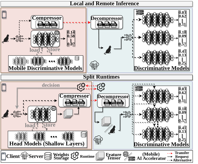
Figure 1: Prediction with On/Offloading and Split Runtimes

Nevertheless, both SC approaches discussed in section 2.2 are only conditionally applicable. In particular, split Runtimes reduce server-side computation for inference tasks with off-the-shelf models by onloading and executing shallow layers at the client. This approach introduces two major limitations.

First, when the latency is crucial, this is only sensible if the time for client-slide execution, transferring the features, and remotely executing the remaining layers is less than the time of directly offloading the task. Consequently, more recent work [26, 25, 27] relies on carefully calibrated dynamic decision mechanisms that periodically measure external and internal conditions (e.g., client state, hardware specifications, and network conditions) to measure ideal split points or whether direct offloading is preferable. Second, since the shallow layers must match the deeper layers, split runtimes cannot accommodate applications with complex requirements which are a common justification for MEC (e.g., MAR). Constrained clients would need to swap weights from the storage in memory each time the prediction model changes to classify from a different set of labels. Worse, the layers must match even for models predicting the same classes with closely related architectures (e.g., ResNet50 and ResNet101). Hence, it is particularly challenging to integrate split runtimes into systems that can increase the resource efficiency of servers by adapting to shifting and fluctuating client conditions [35, 36]. For example, when a client specifies a target accuracy and a tolerable lower bound, the system could select a ResNet101 that can hit the target accuracy but may temporarily fall back to a ResNet50 to ease the load when necessary.

3.2 Execution Times with Resource Asymmetry

Table I summarizes the execution times of ResNet variants that classify a single tensor with dimensions $3\times 224\times 224$ to demonstrate the limitation incurred by partitioning execution of a model when there is considerable resource asymmetry between a client and a server. Specifically, the client is an Nvidia Jetson NX2 equipped with an AI accelerator, and the server hosts an RTX 3090. Section 6 details evaluation setup and hardware configuration.

TABLE I: Execution Times of Split Models

Model	Split Index	Head [NX2] (ms)	Head [3090] (ms)	Tail [3090] (ms)	Rel. Exec. [NX2] (%)	Contribution [NX2] (%)
	Stem	1.5055	0.1024	4.9687	23.25	0.037
ResNet50	Stage 1	8.2628	0.9074	4.0224	67.26	0.882
	Stem	1.5055	0.1024	9.8735	13.23	0.021
ResNet101	Stage 1	8.2628	0.9074	8.9846	47.91	0.506
	Stem	1.5055	0.1024	14.8862	9.18	0.015
ResNet152	Stage 1	8.2628	0.9074	13.8687	37.34	0.374

Like other widespread architectural families, ResNets organize their layers into four top-level layers, while the top-grained ones recursively consist of finer-grained ones. The terminology differs for architectures, but for the remainder of this work, we will refer to top-level layers as stages and the coarse-grained layers as blocks.

Split point stem assigns the first preliminary block as the head model. It consists of a convolutional layer with batch normalization [37] and ReLU activation, followed by a maxpool. Split point stage 1 additionally assigns the first stage to the head.

Notice how the shallow layers barely constitute the overall computation even when the client takes more time to execute the head than the server for the entire model. Further, compare the percentage of total computation time and relate them to the number of parameters. At best, the client contributes to 0.02% of the model execution when taking 9% of the total computation time and may only contribute 0.9% when taking 67% off the computation time.

Despite a reasonably powerful mobile-friendly AI accelerator, it is evident that utilizing client-side resources to aid a server is inefficient. Hence, SC methods commonly include some form of quantization and data size reduction.

3.3 Feature Tensor Dimensionality and Quantization

To further explain the intuition of our claims and present some preliminary empirical evidence, we conceive a hypothetical SC method that typically starts with some statistical analysis of the output layer as illustrated in Figure 2. Excluding repeating blocks, the feature dimensionality is identical for ResNet50, 101, and 152. The red line marks the cutoff where the size of the intermediate feature tensor is less than the original input. ResNets (including more modern variants), among numerous modern architectures, do not have an early natural bottleneck and will only drop below the cutoff from the first block of the second stage (S3RB1-2). Since executing until S3RB1-2 is only about 0.06% of the model parameters of ResNet152, it may seem like a negligible computational overhead. However, as shown in Table I, even when executing 0.04% of the model, the client will make up 37% of the total computation time.

Nevertheless, more modern methods reduce the number of layers a client must execute with feature tensor quantization and other clever (typically statistical) methods that statically or dynamically prune channels [9].

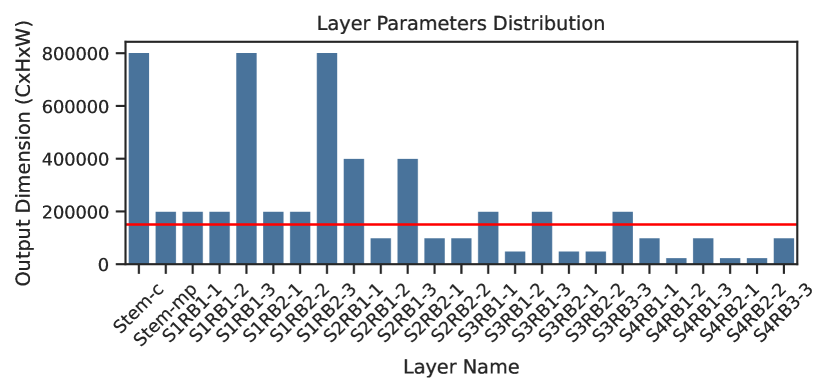
Figure 2: Output Dimensionality Distribution for ResNet

For our hypothetical method, we use the execution times from Table I, except we generously assume that it can apply feature tensor quantization and channel pruning to reduce the expected data size without a loss in accuracy for the ImageNet classification task [38] and with no computational costs. Moreover, we reward the client for executing deeper layers to reflect deterministic bottleneck injection methods, such that the output size of the stem and stage one are 802816 and 428168 bits, respectively. Note that, for stage one, this is roughly a 92% reduction relative to its original FP32 output size at no additional computational cost. Yet, the plots in Figure 3 show that offloading with PNG, let alone more modern lossless codecs (e.g., WebP), will beat SC in total request time, except when the data rate is severely constrained.

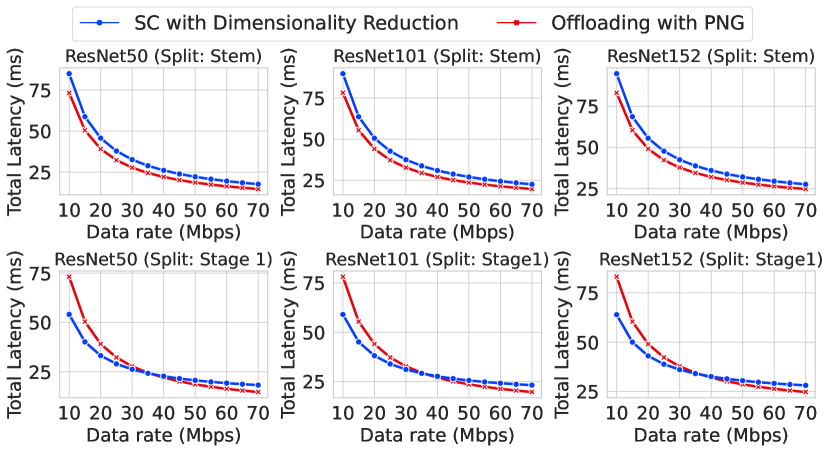
Figure 3: Inference Latency for SC and Offloading

Evidently, using reasonably powerful energy-efficient AI accelerators to execute the shallow layers of a target model is not an efficient use of client-side resources.

3.4 The advantage of learned methods

In a narrow sense, most SC more modern methods consider minimizing transmitting data with feature tensor quantization and other clever (typically statistical) methods that statically or dynamically prune channels, which we reflected with our hypothetical SC method.

While dimensionality reduction can be seen as a crude approximation to compression, it is not equivalent to it [17]. With compression, the aim is to reduce the entropy of the latent under a prior shared between the sender and the receiver [14]. Dimensionality reduction (especially channel pruning) may seem effective when evaluating simple datasets (e.g., CIFAR-10 [39]). However, this is more due to the overparameterization of deep neural networks. Precisely, for a simple task, we can prune most channels or inject a small autoencoder for dimensionality reduction at the shallow layers that may appear to achieve unprecedented compression rates relative to the unmodified head’s feature tensor size. In Section 6.3.7, we will show that methods may seem to work reasonably well on a simple dataset while completely faltering on more challenging datasets.

From an information-theoretic point of view [40], feature tensor (especially non-spatial) dimensionality to assert whether it is a suitable bottleneck is not an ideal measure. Instead, we should consider the information content of the feature tensor. Notably, due to the data processing inequality, as Section 4.1 will elaborate on, the information content of a feature tensor will always be at most as high as the unprocessed input respective to the task. Although dimensionality reduction across spatial dimensions is an effective inductive bias to force a network to discern signals from noise during optimization,

When treating the model itself as a black box, the raw output size measured as $C\times H\times W\times\text{Precision}$ is not a suitable approximation of the data’s entropy, i.e., it is not a meaningful way to assert whether a layer may be a split point. Conversely, with learned approaches, we can optimize a model to compress the input according to its information content and be selective toward the signals we require for tasks we are interested in. Moreover, in Section 6.3.6, we show that with learned transforms and a parametric entropy model, increasing the latent dimensionality, reduces the compressed data size.

To summarize, the potential of SC is inhibited by primarily focusing on shifting parts of the model execution from the server to the client. SC’s viability is not determined by how well they can partially compute a split network but by how well they can reduce the input size. Therefore, we pose the following question: Is it more efficient to focus the local resources exclusively on compressing the data rather than executing shallow layers of a network that would constitute a negligible amount of the total computation cost on the server?

In Figure 4, we sketch predictions with our proposed approach.

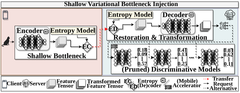
Figure 4: Prediction with Variational Bottleneck Injection

There are two underlying distinctions to common SC methods. First, the model is not split between the client and the server. Instead, it deploys a lightweight encoder, and the decoder replaces the shallow layers, i.e., the discriminative model is split within the server. The decoder’s purpose is to restore and transform the compressed signals and may match multiple backbones and tasks.

Second, compared to split runtimes, the decision to apply the compression model may only depend on internal conditions. It can decouple the client from any external component (e.g., server, router). Ideally, applying the encoder should always be preferable if a mobile device has the minimal required resources. Still, since our method does not alter the backbones, we do not need to serve additional models to accommodate clients that cannot apply the encoder. We can simply route the input to the original input layer, similar to split runtimes, without a runtime that influences client decisions based on external conditions.

This work aims to demonstrate that advancements in energy-efficient AI accelerators for providing constrained clients with demanding requirements (low latency, high accuracy) access to state-of-the-art foundational models are best leveraged with neural compression methods. The following describes the limitations of existing work for constrained devices which we must address to conceive a method suitable for MEC.

4 Problem Formulation

The goal is for constrained clients to request real-time predictions from a large DNN while maximizing resource efficiency and minimizing bandwidth consumption with compression methods. Figure 5 illustrates the possible approaches when dedicating client resources exclusively for compression.

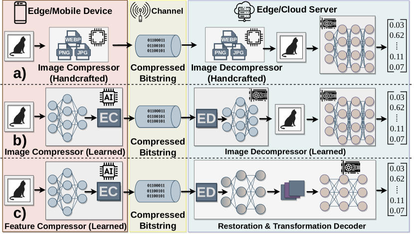
Figure 5: Utilizing Client Resources for (Learned) Codecs

Strategy a) corresponds to offloading strategies with CPU-bound handcrafted codecs. Although learned methods can achieve considerably lower bitrates with comparable distortion than commonly used handcrafted codecs [14], we must consider that the latency overhead incurred by the DNNs (even if executed on AI accelerators) may dominate the reduced transfer time. Strategy b) represents recent LIC models outperforming handcrafted baselines but relying on large DNNs and other complex mechanisms. Strategy c) is our advocated method with an embeddable variational feature compression method and draws from the same underlying Nonlinear Transform Coding (NTC) framework as b). It may seem straightforward to reduce the size of LIC models by prioritizing information sufficient for a particular set of tasks rather than reconstructing the original input. Nevertheless, the challenge is to reduce enough overhead while achieving sufficiently low bitrates without sacrificing predictive strength to make variational compression models suitable for real-time prediction with limited client resources and varying network conditions.

Specifically, to overcome the limitations of SC methods described in Section 3, in addition to offloading with strategy a) and b), (i) we require a resource-conscious encoder that is maximally compressive about a useful representation without increasing the predictive loss. Additionally, (ii) the decoder should exploit the available server-side resources but still incur minimal overhead on the backbone. Lastly, (iii) a compression model should fit for different downstream tasks and architectural families (e.g., CNNs or Vision Transformers) .

Our solution approach in Section 5 must focus on two distinct but intertwined aspects. First is an appropriate training objective for feature compression with limited model capacity. The second concerns a practical implementation by introducing an architectural design heuristic for edge-oriented variational autoencoders. Hence, the following formalizes the properties of a suitable objective function and describes why related existing methods are unsuitable for SVBI.

4.1 Rate-Distortion Theory for Model Prediction

By Shannon’s rate-distortion theory [41], we seek a mapping bound by a distortion constraint from a random variable (r.v.) $X$ to an r.v. $U$, minimizing the bitrate of the outcomes of $X$. More formally, given a distortion measure $\mathcal{D}$ and a distortion constraint $D_{c}$, the minimal bitrate is

$$\underset{P_{U|X}}{\mathrm{min}}\;I(X;U)\;\text{s.t.}\;\mathcal{D}(X,U)\leq D_{c}$$ (1)

where $I(X;U)$ is the mutual information and is defined as

$$\mathrm{I}(X;U)=\int\int p(x,u)\log\left(\frac{p(x,u)}{p(x)p(u)}\right)dxdz$$ (2)

In lossy image compression, $U$ is typically the reconstruction of $\tilde{X}$ of the original input, and the distortion is some sum of squared errors $d(x,\tilde{x})$. Since the r-d theory does not restrict us to reconstruction [42], we can apply distortion measures relevant to M2M communication. Notably, when our objective is to minimize predictive loss rather than reconstructing the input, we keep information that may be important for human perception but excessive for model predictions.

To intuitively understand the potential to discard significantly more information for discriminative models, consider the Data Processing Inequality (DPI). For any 3 r.v.s $X,Y,Z$ that form a Markov chain $X\leftrightarrow Y\leftrightarrow Z$ where the following holds:

$$I(X;Y)\geq I(X;Z)$$ (3)

Then, describe the information flow in an n-layered sequential DNN, layer with the information path by viewing layered neural networks as a Markov chain of successive representations [43]:

$$I(X;Y)\geq I(R_{1};Y)\geq I(R_{2};Y)\geq\dots I(R_{n};Y)\geq I(\tilde{Y};Y)$$ (4)

In other words, due to the DPI, the final representation before a prediction $R_{n}$ cannot have more mutual information with the target than the input $X$ and typically has less. In particular, for discriminative models for high-level vision tasks that map a high dimensional input vector with strong pixel correlations to a small set of labels, we can expect $I(X;Y)\gg I(\tilde{R_{n}},Y)$.

4.2 From Deep to Shallow Bottlenecks

When the task is to predict the ground-truth labels Y from a joint distribution $P_{X,Y}$, the rate-distortion objective is essentially given by the information bottleneck principle [10]. By relaxing the (1) with a lagrangian multiplier, the objective is to maximize:

$$I(Z;Y)-\beta I(Z;X)$$ (5)

Specifically, an encoding $Z$ should be a minimal sufficient statistic of $X$ respective $Y$, i.e., we want $Z$ to contain relevant information regarding $Y$ while discarding irrelevant information from $X$. Practical implementations differ by the target task and how they approximate (5). For example, an approximation of $I(Z;Y)$ for an arbitrary classification task the conditional cross entropy (CE) [11]:

$$\mathcal{D}=H(P_{Y},P_{\tilde{Y}|Z})$$ (6)

Unsurprisingly, using (6) for estimating the distortion measure in (5) for end-to-end optimization of a neural compression model is not a novel idea (Section 2.1.2). However, a common assumption in such work is that the latent variable is the final representation $R_{n}$ before performing the prediction, i.e., the encoder must consist of an entire backbone model which we refer to as Deep Variational Information Bottleneck Injection (DVBI). Conversely, we work with resource-constrained clients, i.e., to conceive lightweight encoders, we must shift the bottleneck to the shallow layers, which we refer to as Shallow Variational Bottleneck Injection (SVBI). Intuitively, the existing methods for DVBI should generalize to SVBI should, e.g., approximating the distortion term with (6) as in [18]. Although by shifting the bottleneck to the shallow layers, the encoder has less capacity for finding a minimal sufficient representation, the objective is still an approximation of (1). Yet, as we will show in Section 6.3.7, applying the objective from [18] will result in incomparably worse results for shallow bottlenecks.

In the following, elaborate on Head Distillation (HD)  [30, 31] that poses an objective that is a suboptimal approximation of (1), but surprisingly yields significantly better results. Moreover, we bridge the gap between deep and shallow bottleneck injection by formulating the VIB objective for HD.

4.3 Head Distilled Deep Variational IB

Ideally, the bottleneck is embeddable in an existing predictor $P_{\mathcal{T}}$ without decreasing the performance. Therefore, it is not the hard labels $Y$ that define the task but the soft labels $Y_{\mathcal{T}}$. For simplicity, we handle the case for one task and defer how SVBI naturally generalizes to multiple downstream tasks and DNNs to Section 6.3.5.

To perform SVBI, take a copy of $P_{\mathcal{T}}$. Then, mark the location of the bottleneck by separating the copy into a head $\mathcal{P}_{h}$ and a tail $\mathcal{P}_{t}$. Importantly, both parts are deterministic, i.e., for every realization of r.v. $X$ there is a representation $\mathcal{P}_{h}(x)=h$ such that $\mathcal{P}_{\mathcal{T}}(x)=\mathcal{P}_{h}(\mathcal{P}_{t}(x))$. Lastly, replace the head with an autoencoder and a parametric entropy model. The encoder is deployed at the sender, the decoder at the receiver, and the entropy model is shared.

We distinguish between two optimization strategies to train the bottleneck’s compression model. First, is direct optimization corresponding to the DVIB objective in (5), except we replace the CE with the standard KD loss [44] to approximate $I(Z;Y)$. Second is indirect optimization and describes HD with the objective:

$$I(Z;H)-\beta\;I(Z;X)$$ (7)

Unlike the former, the latter does not directly correspond to (1) for a representation $Z$ that is a minimal sufficient statistic of $X$ respective $Y_{\mathcal{T}}$. Instead, it replaces $Y$ with a proxy task for the compression model to replicate the output of the replaced head, i.e., training methods approximating (7) optimize for a $Z$ that is a minimal sufficient statistic of $X$ respective $H$. Figure 6 illustrates the difference between estimating the objectives (5) and (7). Intuitively, with faithful replication of $H$, the partially modified DNN has an information path equivalent to its unmodified version. A sufficient statistic retains the information necessary to replicate the input for a deterministic tail, i.e., the final prediction does not change. The problem of (7) is that it is a suboptimal approximation of (1). Although sufficiency holds, it does not optimize $Z$ respective $Y_{\mathcal{T}}$. The marginal distribution of $Y_{\mathcal{T}}$ now arises from the r.v. $X$ and the parameters of $\mathcal{P}_{\mathcal{T}}$. Moreover, since maximizing $I(Z;H)$ is only a proxy objective for $I(Z;Y_{\mathcal{T}})$, it corresponds to the Markov chain $Y_{\mathcal{T}}\leftrightarrow H\leftrightarrow X\leftrightarrow Z$. Notice how $X$ is now conditional independent of $Y_{\mathcal{T}}$. Consequently, when training a compression model with (7), we skew the rate-distortion optimization towards a higher rate than necessary by setting the lower bound for the distortion estimation too high.

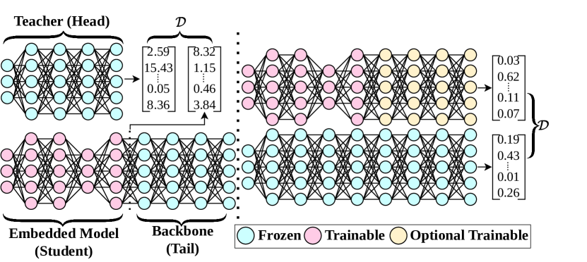
Figure 6: Bottom: direct optimization. Top: Head Distillation

5 Solution Approach

We embed a stochastic compression model that we jointly optimize with an entropy model. Categorically, we follow NTC [14] to implement a neural compression algorithm. For an image vector $x$, we have a parametric analysis transform $g_{a}(x;\phi_{g})$ maps $x$ to a latent vector $z$. Then, a quantizer $Q$ discretizes $z$ to $\bar{z}$, such that an entropy coder can use the entropy model to losslessly compress $\bar{z}$ to a sequence of bits.

It may seem redundant to have a synthesis transform. Instead, we could directly feed the encoder output to the tail of a backbone model. However, this locks the encoder to only a single backbone and disregards the server resources. Thus, we start diverging from NTC for image compression. As shown in Figure 7, rather than an approximate inverse of the analysis, the parametric synthesis transforms $g_{s}(\bar{z};\theta_{g})$ maps $\bar{z}$ to a representation $\tilde{h}$ that is suitable for various tail predictors and downstream tasks.

Figure 7: Diagram of Model Components

5.1 Loss Function for End-to-end Optimization

Our objective resembles variational image compression optimization, as introduced in [15, 16]. Further, we favor HD over direct optimization as a distortion measure, as the former yields considerably better results even with a suboptimal loss function (Section 6.3.7).

Analogous to variational inference, we approximate the intractable posterior $p(\tilde{z}|x)$ with a parametric variational density $q(\tilde{z}|x)$ as follows (excluding constants):

$$\mathbb{E}_{\boldsymbol{x}\sim p_{\boldsymbol{x}}}D_{\mathrm{KL}}\left[q\|p_{\tilde{\boldsymbol{z}}\mid\boldsymbol{x}}\right]=\mathbb{E}_{\boldsymbol{x}\sim p_{\boldsymbol{x}}}\mathbb{E}_{\tilde{\boldsymbol{z}}\sim q}[\underbrace{-\mathrm{log}\;p(x|\tilde{z})}_{\text{ distortion}}-\overbrace{\mathrm{log}\;p(\tilde{z})}^{\text{weighted rate}}]$$ (8)

By assuming a gaussian distribution such that the likelihood of the distortion term is given by

$$P_{x|\tilde{z}}(x\;|\;\tilde{z},\theta_{g})=\mathcal{N}(x\;|\;g_{s}(\tilde{z};\theta_{g}),\;\mathbf{1})$$ (9)

we can use the square sum of differences between $h$ and $\tilde{h}$ as our distortion loss.

The rate term describes the cost of compressing $\tilde{z}$. Analogous to the LIC methods discussed in Section 2.1, we apply uniform quantization $\bar{z}=\lfloor\tilde{z}\rceil$. Since discretization leads to problems with the gradient flow, we apply a continuous relaxation by adding uniform noise $\eta\;\thicksim\;\mathcal{U}(-\frac{1}{2},\frac{1}{2})$. Combining the rate and distortion term, we derive the loss function for approximating objective (7) as

$$\mathcal{L}_{\mathrm{}}=\|\mathcal{P}_{h}(x)\text{ - }(g_{s}(g_{a}(x;\phi_{g})+\eta;\theta_{g})\|^{2}_{2}+\beta\;\mathrm{log}(g_{a}(x;\theta_{g})+\eta)$$ (10)

Note, in the relaxed lagrangian of (1), the weight is on the distortion while we weight the rate term to align closer to the variational information bottleneck objective. Moreover, omitting the second term $(\beta=0)$ and the entropy model would result in the head distillation objective for deterministic bottleneck injection.

We will show that the loss function (10) can yield strong results, despite corresponding to the objective in (7), i.e., it is only a suboptimal approximation of (1) using $H$ as a proxy target. In the previous subsection, we established that as the remaining layers further process a representation $h$, its information content decreases monotonously. Intuitively, the shallow layers extract high-level features, while deeper layers are more focused. Hence, the suboptimality stems from treating every pixel of $H$ equally crucial to the remaining layer. The implication here is that the MSE in (10) overly strictly penalizes pixels at spatial locations which contain redundant information that later layers can safely discard. Contrarily, the loss may not penalize the salient pixels enough when $\tilde{h}$ is numerically close to $h$.

5.2 Saliency Guided Distortion

We can improve the loss in (10) by introducing additional signals that regularize the distortion term. The challenge is finding a tractable method that emphasizes the salient pixels necessary for multiple instances of a high-level vision task (e.g., classification on various datasets and labels). Moreover, the methods’ overhead should only impact train time, i.e., it should not introduce any additional model components or operations during inference.

HD is an extreme form of Hint Training (HT) [45, 46] where the hint becomes the primary objective rather than an auxiliary regularization term. Sbai et al. perform deterministic bottleneck injection with HD using the suboptimal distortion term [31]. Nevertheless, their method only considers crude dimensionality reduction without a parametric entropy model as an approximation to compression, i.e., it is generalized by the loss in (1)$(\beta=0$). Matsubara et al. add further hints from the deeper layers by extending the distortion term with the sum of squared between the deeper layers [30, 21]:

This approach has several downsides besides prolonged train time. In particular, even if (10) could approximate the objective in (1), the distortion term may now dominate the rate term, i.e., without exhaustively tuning the hyperparameters for each distortion term, the optimization algorithm should favor converging towards local optima. We show in Section 6.3.2 that pure HD can significantly outperform this method using the loss in Equation 1 without the hints from the deeper layers.

Ideally, we could improve the performance with signals from deeper layers near the bottleneck. The caveat is that the effectiveness of knowledge distillation decreases for teachers when the student has considerably less capacity than the teacher [45]. Hence, we should not directly introduce hints at the encoder. Instead, we regularize the distortion term with class activation mapping (CAM) [47].

Although CAMs are typically used to improve the explainability of DNNs, we use a variant of Grad-CAM [48] for generating saliency maps to measure a spatial location’s importance at any stage. Figure 8 illustrates some examples of saliency maps when averaged over the deeper backbone stages.

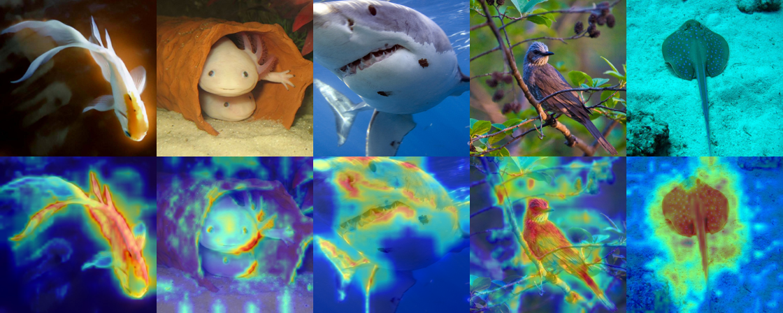
Figure 8: Extracted Saliency Maps using Grad-CAM

Specifically, for each sample, we can derive a vector $\mathcal{S}$, where each $s_{i}\in\mathcal{S}$ is a weight term for a spatial location salient about the conditional probability distributions of the remaining tail layers. Then, we should be able to improve the rate-distortion performance by regularizing the distortion term in (10) with

$$\mathcal{L}_{\mathrm{distortion}}=\gamma_{1}\cdot\mathcal{L}_{1}+\gamma_{2}\cdot s_{i}\cdot\frac{1}{N}\sum_{i}(h_{i}-\tilde{h}_{i})^{2}$$ (11)

Where $\mathcal{L}_{1}$ is the distortiont term from Equation 10, and $\gamma_{1},\gamma_{2}$ are nonnegative real numbers summing to $1$. We default to $\gamma_{1}=\gamma_{2}=\frac{1}{2}$ in our experiments.

Figure 9 describes our final training setup. Note that we only require computing the CAM maps once, and they are architecturally agnostic towards the encoder, i.e., we can re-use them to train various compression models.

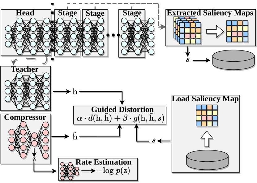
Figure 9: Training Setup

5.3 Network Architecture

The beginning of this section broke down our aim into three problems. We addressed the first with SVBI and proposed a novel training method for low-capacity models. To not inflate the significance of our contribution, we refrain from including efficient neural network components based on existing work in efficient neural network design. A generalizable resource-asymmetry-aware autoencoder design remains; components should be reusable and attachable to at least directly related network architectures once trained.

5.3.1 Model Taxonomy

We introduce a minimal taxonomy described in Figure 10 for our approach. The top-level, Archtype, describes the primary inductive bias of the model. Architectural families describe variants (e.g., ResNets such as ResNet, Wide ResNet, ResNeXt [49], etc.). Lastly, directly related refers to the same architecture of different sizes (e.g., Swin-T, Swin-S, Swin-B, etc.).

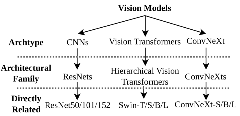
Figure 10: Simple Taxonomy with Minimal Example

The challenge is to conceive a design heuristic that can exploit the available server resources to aid the lightweight encoder with minimal overhead on the prediction task. We assume that, after training an embedded compression model with one particular backbone as described in Section 5.1, it is possible to reuse the encoder or decoder for different backbones with little effort based on the following two observations.

5.3.2 Bottleneck Location by Stage Depth

First is how most modern DNNs consist of an initial embedding followed by a few stages (Described in Section 3.1). Within directly related architectures, the individual components are identical. The difference between variants is primarily the embed dimensions or the block ratio of the deepest stages. For example, the block ratio of ResNet-50 is 3:4:6:3, while the block ratio of ResNet-101 is 3:4:23:3. Therefore, the stage-wise organization of models defines a natural interface for SVBi. For the remainder of this work, we define the shallow layers as all the layers before the stage with the most blocks.

5.3.3 Decoder Blueprint by Inductive Bias

This second observation is how archetypes introduce different inductive biases (e.g., convolutions versus attention modules with sliding windows), leading to diverging representations among non-related architectures. Thus, we should not disregard architecture-induced bias by directly repurposing neural compression models for SC.

For example, a scaled-down version of Ballé et al.’s [15] convolutional neural compression model can yield strong rate-distortion performance for bottlenecks reconstructing a convolutional layer [20] of a discriminative model. However, we will show that this does not generalize to other architectural families, such as hierarchical vision transformers [50].

One potential solution is to use identical components for the compression model from a target network. While this approach may be inconsequential for decoders, given the homogeneity of server hardware, it is inadequate for encoders due to the heterogeneity of edge devices. Vendors have varying support for the basic building blocks of a DNN, and particular operations may be prohibitively expensive for the client.

Consequently, regardless of the decoder architecture, we account for the heterogeneity with a universal encoder composed of three downsampling residual blocks of two stacked $3\times 3$ convolutions, totaling around 140k parameters. Since the mutual information between the original input and shallow layers is still high, it should be possible to add a decoder that maps the representation of the encoder to one suitable for different architectures based on invariance towards invertible transformations of mutual information. Specifically, for invertible functions $\phi,\psi$, it holds that:

$$I(X;Y)=I(\phi(X);\psi(Y))$$ (12)

Specifically, we introduce decoder blueprints for directly related architectures. Blueprints use the same components as target backbones, with some further considerations we describe in the following.

5.3.4 Resource-Asymmetry Aware Network Design

The number of parameters for conventional autoencoders is typically comparable between the encoder and decoder. Increasing the decoder parameters does not change the inability to recover lost signals (Section 4.1), i.e., it does not offset the limited encoder capacity for accurately distinguishing between valuable and redundant information.

Nevertheless, when optimizing the entire compression pipeline simultaneously, the training algorithm should consider the decoder’s restoration ability, which in turn should help the encoder parameters converge towards finding a minimal sufficient statistic respective to the task. Hence, Inspired by [51], we partially treat decoding as an image restoration problem and add restoration blocks with optional upsampling (e.g., deconvolutions or PixelShuffle [52]) between backbone-specific transformation blocks. In other words, our decoder is a restoration model we jointly train with the encoder, such that the optimization process is informed on how faint the bottleneck’s output signal can be to remain recoverable. The decoder size can be as large as the pruned layers, i.e., our method does not reduce computational time on the server.

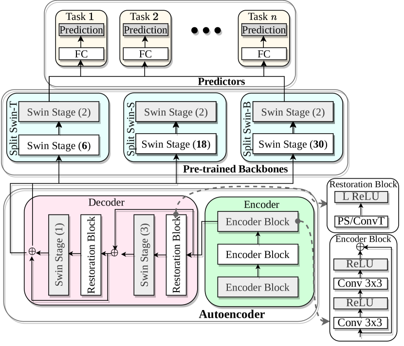
Figure 11: Reference Implementation with Swin backbones

To summarize, our network architecture is a general design heuristic, i.e., the individual components are interchangeable with the current state-of-the-art building blocks for vision models. Figure 11 illustrates one of the reference implementations we will use for our evaluation in Section 6. The number in parentheses represents stage depth. We include implementations of other reference blueprints in the accompanying repository with descriptive configurations. Multiple downstream tasks are supported by attaching different predictors on the pre-trained backbones from foundational models.

6 Evaluation

6.1 Training & Implementation Details

We optimize our compression models initially on the 1.28 million ImageNet [38] training samples for 15 epochs, as described in section 5.1 and section 5.2, with some slight practical modifications for stable training. We use Adam optimization [53] with a batch size of $16$ and start with an initial learning rate of $1\cdot 10^{-3}$, then gradually lower it to $1\times 10^{-6}$ with an exponential scheduler.

We aim to minimize bitrate without sacrificing predictive strength. Hence, we first seek the lowest $\beta$ resulting in lossless prediction.

To implement our method, we use PyTorch [54], CompressAI [55] for entropy estimation and entropy coding, and pre-trained backbones from PyTorch Image Models [56]. All baseline implementations and weights were either taken from CompressAI or the official repository of a baseline. To compute the saliency maps, we use a modified XGradCAM method from the library in [57] and include necessary patches in our repository. Lastly, to ensure reproducibility, we use torchdistill [58].

6.2 Experiment Setting

The experiments reflect the deployment strategies illustrated in Figure 5 and Figure 4. Ultimately, we must evaluate whether FrankenSplit enables latency-sensitive and performance-critical applications. Regardless of the particular task, a mobile edge client requires access to a DNN with high predictive strength on a server. Therefore, we must show whether FrankenSplit adequately solves two problems associated with offloading high-dimensional image data for real-time inference tasks. First, whether it considerably reduces the bandwidth consumption compared to existing methods without sacrificing predictive strength. Second, whether it improves inference times over various communication channels, i.e., it must remain competitive even when stronger connections are available.

Lastly, FrankenSplit should still be applicable as newer DNN architectures emerge, i.e., the evaluation should assess whether our method generalizes to arbitrary backbones. However, since it is infeasible to perform exhaustive experiments on all existing visual models, we focus on three well-known representatives and a subset of their variants instead. Namely, (i) ResNet [59] for classic residual CNNs. (ii) Swin Transformer [50] for hierarchical vision transformers, which are receiving increasing adaptation for a wide variety of vision tasks. (iii) ConvNeXt [60] for modernized state-of-the-art CNNs. Table II summarizes the relevant characteristics of the unmodified backbones subject to our experiments.

TABLE II: Overview of Backbone Performance on Server

Backbone	Ratios	Params	Inference (ms)	Top-1 Acc. (%)
Swin-T	2:2:6:2	28.33M	4.77	81.93
Swin-S	2:2:18:2	49.74M	8.95	83.46
Swin-B	2:2:30:2	71.13M	13.14	83.88
ConvNeXt-T	3:3:9:3	28.59M	5.12	82.70
ConvNeXt-S	3:3:27:3	50.22M	5.65	83.71
ConvNeXt-B	3:3:27:3	88.59M	6.09	84.43
ResNet-50	3:4:6:3	25.56M	5.17	80.10
ResNet-101	3:4:23:3	44.55M	10.17	81.91
ResNet-152	3:8:36:3	60.19M	15.18	82.54

6.2.1 Baselines

Since our work aligns closest to learned image compression, we extensively compare FrankenSplit with learned and handcrafted codecs applied to the input images, i.e., the input to the backbone is the distorted output. Comparing task-specific methods to general-purpose image compression methods may seem unfair. However, FrankenSplit’s universal encoder has up to 260x less trainable parameters and further reduces overhead by not including side information or a sequential context model.

The naming convention for the learned baselines is the first author’s name, followed by the entropy model. Specifically, we choose the work by Balle et al. [15, 16] and Minnen et al. [17] for LIC methods since they represent foundational milestones. Complementary, we include the work by Cheng et al. [61] to demonstrate improvements with architectural enhancement.

As the representative for disregarding autoencoder size to achieve state-of-the-art r-d performance in LIC, we chose the work by Chen et al. [62] Their method differs from other LIC baselines by using a partially parallelizable context model, which trades off compression rate with execution time according to the configurable block size. However, due to the large autoencoder, we found evaluating the inference time on constrained devices impractical when the context model is purely sequential and set the block size to 64x64. Additionally, we include the work by Lu et al. [63] as a milestone of the recent effort on efficient LIC with reduced autoencoders but only for latency-related experiments since we do not have access to the trained weights.

As a baseline for the state-of-the-art SC, we include the Entropic Student (ES) [20, 21]. Crucially, the ES demonstrates the performance of directly applying a minimally adjusted LIC method for feature compression without considering the intrinsic properties of the problem domain we have derived in Section 4.1. One caveat is that we intend to show how FrankenSplit generalizes beyond CNN backbones, despite the encoder’s simplistic CNN architecture. Although Matsubara et al. evaluate the ES on a wide range of backbones, most have no lossless configurations. However, comparing bottleneck injection methods using different backbones is fair, as we found that the choice does not significantly impact the rate-ddistortion performance. Therefore, for an intuitive comparison, we choose ES with ResNet-50 using the same factorized prior entropy model as FrankenSplit.

We separate the experiments into two categories to assess whether our proposed method addresses the abovementioned problems.

6.2.2 Criteria rate-distortion performance

We primarily measure the bitrate in bits per pixel (bpp) which is sensible because it permits directly comparing models with different input sizes. Choosing a distortion measure to draw meaningful and honest comparisons is challenging for feature compression. Unlike evaluating reconstruction fidelity for image compression, PSNR or MS-SSIM does not provide intuitive results regarding predictive strength. Similarly, adhering to the customs of SC by reporting absolute values, such as top-1 accuracy, gives an unfair advantage to experiments conducted on higher capacity backbones and veils the efficacy of a proposed method. Consequently, we evaluate the distortion with the relative measure predictive loss. To ensure a fair comparison, we give the LIC and handcrafted baselines a grace threshold of 1.0% top-1 accuracy, considering it is possible to mitigate some predictive loss incurred by codec artifacts [64]. For example, if a model has a predictive loss of 1.5% top-1 accuracy, we report it as 0.5% below our definition of lossless prediction. However, for FrankenSplit, we set the grace threshold at 0.4%, reflecting the configuration with the lowest predictive loss of the ES. Note that the ES improves rate-distortion performance by finetuning the backbone weights by applying a secondary training stage. In contrast, we put our work at a disadvantage by training FrankenSplit exclusively with the methods introduced in this work.

6.2.3 Measuring latency and overhead

The second category concerns with execution times of prediction pipelines with various wireless connections. To account for the resource asymmetry in MEC, we use NVIDIA Jetson boards to represent the capable but resource-constrained mobile client, and the server hosts a powerful GPU. Table III summarizes the hardware we use in our experiments.

TABLE III: Clients and Server Hardware Configuration

Device	Arch	CPU	GPU
Server	x86	16x Ryzen @ 3.4 GHz	RTX 3090
Client (TX2)	arm64x8	4x Cortex @ 2 GHz	Vol. 48 TC
Client (NX)	arm64x8	4x Cortex @ 2 GHz	Pas. 256 CC

6.3 Rate-Distortion Performance

We measure the predictive loss by the drop in top-1 accuracy from Table II using the ImageNet validation set for the standard classification task with 1000 categories. Analogously, we measure filesizes of the entropy-coded binaries to calculate the average bpp. Figure 12 shows rate-distortion curves with the Swin-B backbone. The architecture of FrankenSplit-FP (FS-FP) and FrankenSplit-SGFP (FS-SGFP) are identical. We train both models with the loss functions derived in Section 5.1. The difference is that FS-SGFP is saliency guided, i.e., FS-FP represents the suboptimal HD training method and is an ablation to our proposed solution.

6.3.1 Effect of Saliency Guidance

Although FS-FP performs better than almost all other models, it is trained with the suboptimal objective discussed in Section 4.3. Empirically, this is demonstrated by FS-SGFP outperforming FS-FP on the r-d curve. By simply guiding the distortion loss with saliency maps, we achieve a 25% lower bitrate at no additional cots.

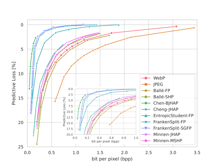
Figure 12: Rate-distortion curve for ImageNet

6.3.2 Comparison to the ES

Even without saliency guidance, FS-FP consistently outperforms ES by a large margin. Specifically, FS-FP and FS-SGFP achieve 32% and 63% lower bitrates for the lossless configuration.

We ensured that our bottleneck injection incurs comparable overhead for a direct comparison to the ES. Moreover, the ES has an advantage due to fine-tuning tail parameters in an auxiliary training stage. Therefore, we attribute the performance gain to the more sophisticated architectural design decisions described in Section 5.3.

6.3.3 Comparison to Image Codecs

For almost all lossy codec baselines, Figure 12 illustrates that FS-(SG)FP has a significantly better r-d performance. Comparing FS-FP to Ballé-FP demonstrates the r-d gain of task-specific compression over general-purpose image compression. Although the encoder of FrankenSplit has 25x fewer parameters, both codecs use an FP entropy model with encoders consisting of convolutional layers. Yet, the average file size of FS-FP with a predictive loss of around 5% is 7x less than the average file size of Ballé-FP with comparable predictive loss.

FrankenSplit also beats modern general-purpose LIC without including any of their complex or heavy-weight mechanisms. The only baseline, FrankenSplit does not convincingly outperform is Chen-BJHAP. Nevertheless, incurred overhead is as vital for real-time inference, which we will evaluate Section 6.4.

6.3.4 Generalization to arbitrary backbones

In the previous, we intentionally demonstrated the rate-distortion performance of FrankenSplit with a Swin backbone since it backs up our claim from Section 5.3 that the synthesis transform can map the CNN encoder output to the input of a hierarchical vision transformer. Nevertheless, we found that the choice of backbone has a negligible impact on the rate-distortion performance. Additionally, due to the relative distortion measure, different backbones will not lead to significantly different rate-distortion curves for the baseline codecs, i.e., when we measure by predictive loss, we get nearly identical results. Arguably, allowing operators to reason in predictive loss is more valuable than by-model absolute values, as it permits measuring whether and how much performance drop clients can expect decoupled from the backbones they use.

The insignificance of teacher choice for rate-distortion performance is consistent with all our claims and findings. With the objective in (7), we learn the representation of a shallow layer, which generalizes well since such representations can retain high mutual information with the original input.

What remains is to demonstrate the necessity of our heuristic regarding inductive bias with decoder blueprints.

TABLE IV: Effect of Blueprints on a Backbone

Blueprint-Backbone	File Size (kB)	Predictive Loss (%)
	8.70	0.00
	5.08	0.40
Swin-Swin	3.19	0.77
	19.05	2.49
	15.07	3.00
ConvNeXt-Swin	10.05	3.35
	22.54	0.82
	18.19	0.99
ResNet-Swin	8.27	1.34

As Section 5.3 detailed, the decoder consists of interchangeable restoration and transformation blocks. Irrespective of the backbone, restoration blocks are residual pixel shuffles or transpose convolutions. Contrarily, the transformation block depends on the target backbone, and we argued that the r-d performance improves when the transformation block induces the same bias as the target backbone. Specifically, we create a synthesis transform blueprint for each of the three architectural families (Swin, ResNet, and ConvNeXt) that results in comparable rate-distortion performance from Figure 12 for their intended variations. For example, for any ConvNeXt backbone variation, we train the bottleneck with the ConvNeXt synthesis blueprint. However, as summarized in Table IV, once we attempt to use the ResNet or ConvNeXt restoration blocks, the rate-distortion performance for the Swin-B is significantly worse. Most notably, the lossless configuration for Swin-Swin has less than half the average file size of ConvNeXt-Swin with 2.49% predictive loss.

6.3.5 Generalization to multiple Downstream Tasks

We argue that SVBI naturally generalizes to multiple downstream tasks for two reasons. First, the head distillation method optimizes our encoder to learn high-level representations, i.e., the mutual information between the bottleneck output and the original input is still high. Additionally, hierarchical vision models are primarily feature extractors. Since the bottleneck learns to approximate the representation from a challenging distribution, embedding the same compression module on backbones or predictors trained for other tasks should be possible. We provide empirical evidence by finetuning a predictor prepared on ImageNet for different datasets.

For FrankenSplit, we applied none or only rudimentary augmentation to evaluate how our method handles a type of noise it did not encounter during training. Hence, we include the Food-101 [65] dataset since it contains noise in high pixel intensities. Additionally, we include CIFAR-100 [39]. Lastly, we include Flower-102 [66] datasets to contrast more challenging tasks.

We freeze the entire compression model trained on the ImageNet dataset and finetune the tails separately for five epochs with no augmentation, a learning rate of $5\cdot 10^{-5}$ using Adam optimization. The teacher backbones achieve an $87.73\%$, $88.01\%$, and $89.00\%$ top-1 accuracy, respectively. Figure 13 summarizes the rate-distortion performance for each task.

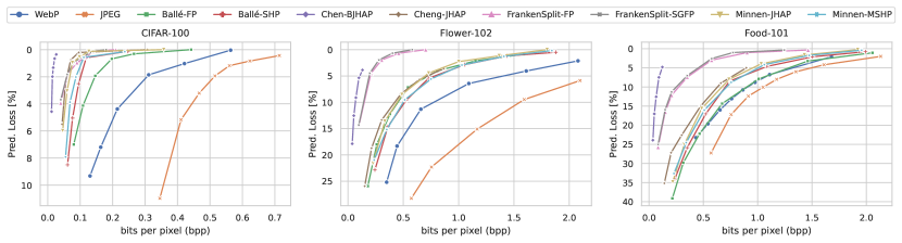
Figure 13: Rate-distortion curve for multiple downstream tasks

Our method still demonstrates clear rate-distortion performance gains over the baselines. More importantly, notice how FS-SGFP outperforms FS-FP on the r-d curve for the Food-101 dataset, with a comparable margin to the ImageNet dataset. Contrarily, on the Flower-102 datasets, there is noticeably less performance difference between them. Presumably, on simple datasets, the suboptimality of HD is less significant. Considering how simpler tasks require less model capacity, the diminishing efficacy of our saliency-guided training method is consistent with our claims and derivations in Section 4. The information of the shallow layer may suffice, i.e., the less necessary the activations of the deeper layers are, the better a minimal sufficient statistic respective $H$ approximates a minimal sufficient statistic respective $Y$.

6.3.6 Effect of Tensor Dimensionality on R-D Performance

In Section 3.3, we argued that tensor dimensionality is not a suitable measure to assess whether it is worthwhile to perform some client-side execution.

To provide further evidence, we implement and train additional instances of FrankenSplit and show results in Figure 14

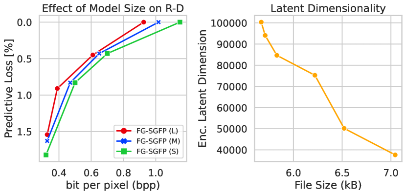
Figure 14: Comparing Effects on Sizes

FS-SGFP(S) is the model with a small encoder ( 140’000 parameters) we have used for our previous results. FS-SGFP(M) and FS-SGFP(L) are medium and large models where we increased the (output) channels $C=48$ to $96$ and $128$, respectively. Besides the number of channels, we’ve trained the medium and large models using the same configurations. On the left, we plot the rate-distortion curves showing that increasing encode capacity naturally results in lower bitrates without additional predictive loss. For the plot on the right, we train further models with $C=\{48,64,96,108,120,128\}$ using the configuration resulting in lossless prediction. Notice how increasing output channels will result in higher dimensional latent tensors $C\times 28\times 28$ but inversely correlates to compressed file size. An obvious explanation is that increasing the encoder capacity will yield more powerful transforms for better entropy coding and uniform quantization.

6.3.7 The Limitations of Direct Optimization for SVBI

In Section 5.1, we mentioned that direct optimization does not work for SVBI as it does for DVBI, where the bottleneck is at the penultimate layer. Specifically, it performs incomparably worse than HD despite the latter’s inherent suboptimality. Contrasting the rate-distortion performance on the simple CIFAR-10 [39] dataset summarized in the left with the rate-distortion performance on the ImageNet dataset on the right in Figure 15 provides empirical evidence. Other than training direct optimization methods for more epochs to account for slower convergence, all models are identical and optimized with the setup described in Section 6.1. On the simple task, SVBI-CE and SVBI-KD yield moderate performance gain over JPEG. Since sufficiency is a necessary precondition for a minimal sufficient statistic which may explain why the objective in (5) does not yield good results when the bottleneck is at a shallow layer, as the mutual information $I(Y;\tilde{Y})$ is not adequately high. This becomes especially evident when the same method entirely falters on the more challenging ImageNet dataset. Despite skewing the rate-distortion objective heavily towards high bitrates, it does not result in $\tilde{H}$ to be a sufficient statistic of $H$.

Since the representation of the last hidden layer and the representation of the shallow layer are so far apart in the information path, there is insufficient information to minimize $\mathcal{D}(H;\tilde{H})$. When the joint distribution $P_{X,Y}$ arises from a simple dataset, $I(Y;\tilde{Y})$ has just enough information to propagate down for the compression model to come close to a sufficient statistic of $Z$ respective $Y$. However, when $P_{X,Y}$ arises from a challenging dataset, where the information content of $I(Y;\tilde{Y})$ is not enough to approximate a sufficient statistic, it performs significantly worse.

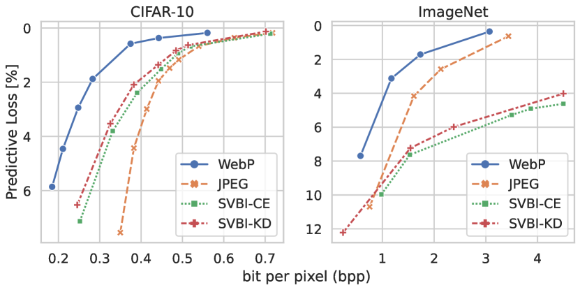
Figure 15: Contrasting the r-d performance

A final observation is that we should not assume feature compression methods demonstrating excellent results on simple tasks will naturally generalize, especially when not supplemented with relative evaluation metrics.

6.4 Prediction Latency and Overhead

We exclude entropy coding from our measurement, since not all baselines use the same entropy coder. For brevity, the results implicitly assume the Swin-B backbone for the remainder of this section. Inference times with other backbones for FrankenSplit can be derived from Table V.

TABLE V: Execution Times of FS (S) with Various Backbones

Backbone	Overhead Prams (%)	Inf. Server+NX (m/s)	Inf. Server+TX2 (m/s)
Swin-T	2.51	7.83	9.75
Swin-S	1.41	11.99	13.91
Swin-B	1.00	16.12	18.04
ConvNeXt-T	3.46	6.83	8.75
ConvNeXt-S	1.97	8.50	10.41
ConvNeXt-B	0.90	9.70	11.62
ResNet-50	3.50	13.16	10.05
ResNet-101	2.01	8.13	15.08
ResNet-152	1.48	18.86	20.78

Analogously, the inference times of applying LIC models for different unmodified backbones can be derived using Table II. Notably, the relative overhead decreases the larger the tail is, which is favorable since we target inference from more accurate predictors.

6.4.1 Computational Overhead

We first disregard network conditions to get an overview of the computational overhead of applying compression models. Table VI summarizes the execution times of the prediction pipeline’s components.

TABLE VI: Inference Pipeline Components Execution Times

Model	Prams Enc./Dec.	Enc. [NX/TX2] (ms)	Dec. (ms)	Full [NX/TX2] (ms)
FrankenSplit	0.14M/ 2.06M	2.92/ 4.87	2.00	16.34/ 18.29
Ballé-FP	3.51M/ 3.51M	27.27/ 48.93	1.30	41.71/ 63.37
Ballé-SHP	8.30M/ 5.90M	28.16/ 50.89	1.51	42.81/ 65.54
Minnen-MSHP	14.04M/ 11.65M	29.51/ 52.39	1.52	44.17/ 67.05
Minnen-JHAP	21.99M/ 19.59M	4128.17/ 4789.89	275.18	4416.7/ 5078.2
Cheng-JHAP	16.35M/ 22.27M	2167.34/ 4153.95	277.26	2457.7/ 4444.3
Lu-JHAP	5.28M/ 4.37M	2090.88/ 5011.56	352.85	2456.8/ 5377.8
Chen-BJHAP	36.73M/ 28.08M	3111.01/ 5837.38	43.16	3167.3/ 5893.6

Enc. NX/TX2 refers to the encoding time on the respective client device. Analogously, dec. refers to the decoding time at the server. Lastly, Full NX/TX2 is the total execution time of encoding at the respective client plus decoding and the prediction task at the server. Lu-JHAP demonstrates how LIC models without a sequential context component are noticeably faster but are still 9.3x-9.6x slower than FrankenSplit despite a considerably worse r-d performance. Comparing Ballé-FP to Minnen-MSHP reveals that including side information only incurs minimal overhead, even on the constrained client. On the server, FrankenSplit’s is slightly slower than some baselines due to the attention mechanism of the decoder blueprint for the swin backbone. However, unlike all other baselines, the computational load of FrankenSplit is near evenly distributed between the client and the server, i.e., FrankenSplit’s design heuristic successfully considers resource asymmetry. The significance of considering resource asymmetry is emphasized by how the partially parallelized context model of Chen-BHJAP leads to faster decoding on the server. Nevertheless, it is slower than other JHAP baselines due to the overhead of the increased encoder size outweighing the performance gain of the blocked context model on constrained hardware.

6.4.2 Competing against Offloading

Unlike SC methods, we do not reduce the latency on the server, i.e., performance gains of FrankenSplit solely stem from reduced transfer times. The average compressed filesize gives the transfer size from the ImageNet validation set.

TABLE VII: Total Latency with Various Wireless Standards

Standard/ Data Rate (Mbps)	codec	Transfer (ms)	Total [TX2] (ms)	Total [NX] (ms)
	FS-SGFP (0.23)	142.59	160.48	158.53
	FS-SGFP (LL)	209.89	227.78	225.83
	Minnen-MSHP	348.85	415.89	393.01
	Chen-BJHAP	40.0	6167.79	3441.41
	WebP	865.92	879.06	879.06
BLE/ 0.27	PNG	2532.58	2545.72	2545.72
	FS-SGFP (0.23)	3.21	21.09	19.15
	FS-SGFP (LL)	4.72	22.61	20.66
	Minnen-MSHP	7.85	74.89	52.01
	Chen-BJHAP	0.9	6128.69	3402.31
	WebP	19.48	32.63	32.63
4G/ 12.0	PNG	56.98	70.13	70.13
	FS-SGFP (0.23)	0.71	18.6	16.65
	FS-SGFP (LL)	1.05	18.93	16.99
	Minnen-MSHP	1.74	68.78	45.9
	Chen-BJHAP	0.2	6127.99	3401.61
	WebP	4.33	17.47	17.47
Wi-Fi/ 54.0	PNG	12.66	25.81	25.81
	FS-SGFP (0.23)	0.58	18.46	16.51
	FS-SGFP (LL)	0.85	18.73	16.78
	Minnen-MSHP	1.41	68.44	45.56
5G/ 66.9	Chen-BJHAP	0.16	6127.95	3401.57
	WebP	3.49	16.64	16.64
	PNG	10.22	23.36	23.36

Using the transfer size, we evaluate transfer time on a broad range of standards. Since we did not include the execution time of entropy coding for learned methods, the encoding and decoding time for the handcrafted codecs is set to 0. The setting favors the baselines because both rely on entropy coding and sequential CPU-bound transforms. Table VII summarizes how our method performs in various standards. Due to space constraints, we only include LIC models with the lowest request latency (Minnen-MSHP) or the lowest compression rate (Chen-BJAHP). Still, with Table VI and the rate-distortion results from the previous subsection, we can infer that the LIC baselines have considerably higher latency than FrankenSplit.

Generally, the more constrained the network is the more we can benefit from reducing the transfer size. In particular, FrankenSplit is up to 16x faster in highly constrained networks, such as BLE. Conversely, offloading with fast handcrafted codecs may be preferable in high-bandwidth environments. Yet, FrankenSplit is significantly better than offloading with PNG, even for 5G. Figure 16 plots the inference latencies against handcrafted codecs using the NX client.

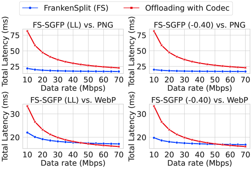
Figure 16: Comparing Effects on Sizes

For stronger connections, such as 4G LTE, it is still 3.3x faster than using PNG. Nevertheless, compared to WebP, offloading seems more favorable when bandwidth is high. Still, this assumes that the rates do not fluctuate and that the network can seamlessly scale for an arbitrary number of client connections. Moreover, kept the encoder as simple and minimal as possible without applying any further architectural optimizations.

7 Conclusion

In this work, we introduced a novel lightweight compression framework to facilitate critical MEC applications relying on large DNNs. We demonstrated that a minimalistic implementation of our design heuristic is sufficient to outperform numerous baselines. However, our method still has several limitations. Notably, it assumes that the client has an onboard accelerator. Moreover, the simplistic Factorized Prior entropy model is not input adaptive, i.e., it does not adequately discriminate between varying inputs. Although adding side information with hypernetworks taken from LIC trivially improves rate-distortion performance, our results show that it may not be a productive approach to directly repurpose existing image compression methods. Hence, conceiving an efficient way to include task-dependent side information is a promising direction.

References

- [1] A. Voulodimos, N. Doulamis, A. Doulamis, E. Protopapadakis, et al., “Deep learning for computer vision: A brief review,” Computational intelligence and neuroscience, vol. 2018, 2018.
- [2] D. W. Otter, J. R. Medina, and J. K. Kalita, “A survey of the usages of deep learning for natural language processing,” IEEE transactions on neural networks and learning systems, vol. 32, no. 2, pp. 604–624, 2020.
- [3] C. Feng, P. Han, X. Zhang, B. Yang, Y. Liu, and L. Guo, “Computation offloading in mobile edge computing networks: A survey,” Journal of Network and Computer Applications, p. 103366, 2022.
- [4] T. Rausch, W. Hummer, C. Stippel, S. Vasiljevic, C. Elvezio, S. Dustdar, and K. Krösl, “Towards a platform for smart city-scale cognitive assistance applications,” in 2021 IEEE Conference on Virtual Reality and 3D User Interfaces Abstracts and Workshops (VRW), pp. 330–335, 2021.
- [5] R. R. Arinta and E. Andi W.R., “Natural disaster application on big data and machine learning: A review,” in 2019 4th International Conference on Information Technology, Information Systems and Electrical Engineering (ICITISEE), pp. 249–254, 2019.
- [6] Q. Xin, M. Alazab, V. G. Díaz, C. E. Montenegro-Marin, and R. G. Crespo, “A deep learning architecture for power management in smart cities,” Energy Reports, vol. 8, pp. 1568–1577, 2022.
- [7] U. Cisco, “Cisco annual internet report (2018–2023) white paper,” Cisco: San Jose, CA, USA, vol. 10, no. 1, pp. 1–35, 2020.
- [8] F. Romero, Q. Li, N. J. Yadwadkar, and C. Kozyrakis, “INFaaS: Automated model-less inference serving,” in 2021 USENIX Annual Technical Conference (USENIX ATC 21), pp. 397–411, USENIX Association, July 2021.
- [9] Y. Matsubara, M. Levorato, and F. Restuccia, “Split computing and early exiting for deep learning applications: Survey and research challenges,” ACM Computing Surveys, vol. 55, no. 5, pp. 1–30, 2022.
- [10] N. Tishby, F. C. Pereira, and W. Bialek, “The information bottleneck method,” 2000.
- [11] Y. Yang, S. Mandt, and L. Theis, “An introduction to neural data compression,” 2022.
- [12] G. LLC, “An image format for the web.”
- [13] V. Goyal, “Theoretical foundations of transform coding,” IEEE Signal Processing Magazine, vol. 18, no. 5, pp. 9–21, 2001.
- [14] J. Ballé, P. A. Chou, D. Minnen, S. Singh, N. Johnston, E. Agustsson, S. J. Hwang, and G. Toderici, “Nonlinear transform coding,” CoRR, vol. abs/2007.03034, 2020.
- [15] J. Ballé, V. Laparra, and E. P. Simoncelli, “End-to-end optimized image compression,” in 5th International Conference on Learning Representations, ICLR 2017, Toulon, France, April 24-26, 2017, Conference Track Proceedings, OpenReview.net, 2017.
- [16] J. Ballé, D. Minnen, S. Singh, S. J. Hwang, and N. Johnston, “Variational image compression with a scale hyperprior,” 2018.
- [17] D. Minnen, J. Ballé, and G. Toderici, “Joint autoregressive and hierarchical priors for learned image compression,” 2018.
- [18] S. Singh, S. Abu-El-Haija, N. Johnston, J. Ballé, A. Shrivastava, and G. Toderici, “End-to-end learning of compressible features,” CoRR, vol. abs/2007.11797, 2020.
- [19] Y. Dubois, B. Bloem-Reddy, K. Ullrich, and C. J. Maddison, “Lossy compression for lossless prediction,” Advances in Neural Information Processing Systems, vol. 34, pp. 14014–14028, 2021.
- [20] Y. Matsubara, R. Yang, M. Levorato, and S. Mandt, “Sc2: Supervised compression for split computing,” 2022.
- [21] Y. Matsubara, R. Yang, M. Levorato, and S. Mandt, “Supervised compression for resource-constrained edge computing systems,” in Proceedings of the IEEE/CVF Winter Conference on Applications of Computer Vision, pp. 2685–2695, 2022.
- [22] Y. Kang, J. Hauswald, C. Gao, A. Rovinski, T. Mudge, J. Mars, and L. Tang, “Neurosurgeon: Collaborative intelligence between the cloud and mobile edge,” ACM SIGARCH Computer Architecture News, vol. 45, no. 1, pp. 615–629, 2017.
- [23] H. Li, C. Hu, J. Jiang, Z. Wang, Y. Wen, and W. Zhu, “Jalad: Joint accuracy-and latency-aware deep structure decoupling for edge-cloud execution,” in 2018 IEEE 24th international conference on parallel and distributed systems (ICPADS), pp. 671–678, IEEE, 2018.
- [24] S. Laskaridis, S. I. Venieris, M. Almeida, I. Leontiadis, and N. D. Lane, “Spinn: synergistic progressive inference of neural networks over device and cloud,” in Proceedings of the 26th annual international conference on mobile computing and networking, pp. 1–15, 2020.
- [25] M. Almeida, S. Laskaridis, S. I. Venieris, I. Leontiadis, and N. D. Lane, “Dyno: Dynamic onloading of deep neural networks from cloud to device,” ACM Transactions on Embedded Computing Systems, vol. 21, no. 6, pp. 1–24, 2022.
- [26] H. Liu, W. Zheng, L. Li, and M. Guo, “Loadpart: Load-aware dynamic partition of deep neural networks for edge offloading,” in 2022 IEEE 42nd International Conference on Distributed Computing Systems (ICDCS), pp. 481–491, 2022.
- [27] A. Bakhtiarnia, N. Milošević, Q. Zhang, D. Bajović, and A. Iosifidis, “Dynamic split computing for efficient deep edge intelligence,” in ICASSP 2023 - 2023 IEEE International Conference on Acoustics, Speech and Signal Processing (ICASSP), pp. 1–5, 2023.
- [28] A. E. Eshratifar, A. Esmaili, and M. Pedram, “Bottlenet: A deep learning architecture for intelligent mobile cloud computing services,” in 2019 IEEE/ACM International Symposium on Low Power Electronics and Design (ISLPED), pp. 1–6, 2019.
- [29] J. Shao and J. Zhang, “Bottlenet++: An end-to-end approach for feature compression in device-edge co-inference systems,” in 2020 IEEE International Conference on Communications Workshops (ICC Workshops), pp. 1–6, 2020.
- [30] Y. Matsubara, S. Baidya, D. Callegaro, M. Levorato, and S. Singh, “Distilled split deep neural networks for edge-assisted real-time systems,” in Proceedings of the 2019 Workshop on Hot Topics in Video Analytics and Intelligent Edges, HotEdgeVideo’19, (New York, NY, USA), p. 21–26, Association for Computing Machinery, 2019.
- [31] M. Sbai, M. R. U. Saputra, N. Trigoni, and A. Markham, “Cut, distil and encode (cde): Split cloud-edge deep inference,” in 2021 18th Annual IEEE International Conference on Sensing, Communication, and Networking (SECON), pp. 1–9, 2021.
- [32] L. Deng, G. Li, S. Han, L. Shi, and Y. Xie, “Model compression and hardware acceleration for neural networks: A comprehensive survey,” Proceedings of the IEEE, vol. 108, no. 4, pp. 485–532, 2020.
- [33] Z. Li, F. Liu, W. Yang, S. Peng, and J. Zhou, “A survey of convolutional neural networks: analysis, applications, and prospects,” IEEE transactions on neural networks and learning systems, 2021.
- [34] K. Han, Y. Wang, H. Chen, X. Chen, J. Guo, Z. Liu, Y. Tang, A. Xiao, C. Xu, Y. Xu, et al., “A survey on vision transformer,” IEEE transactions on pattern analysis and machine intelligence, vol. 45, no. 1, pp. 87–110, 2022.
- [35] F. Romero, Q. Li, N. J. Yadwadkar, and C. Kozyrakis, “Infaas: Automated model-less inference serving.,” in USENIX Annual Technical Conference, pp. 397–411, 2021.
- [36] K. Zhao, Z. Zhou, X. Chen, R. Zhou, X. Zhang, S. Yu, and D. Wu, “Edgeadaptor: Online configuration adaption, model selection and resource provisioning for edge dnn inference serving at scale,” IEEE Transactions on Mobile Computing, pp. 1–16, 2022.
- [37] S. Ioffe and C. Szegedy, “Batch normalization: Accelerating deep network training by reducing internal covariate shift,” in International conference on machine learning, pp. 448–456, pmlr, 2015.
- [38] O. Russakovsky, J. Deng, H. Su, J. Krause, S. Satheesh, S. Ma, Z. Huang, A. Karpathy, A. Khosla, M. Bernstein, et al., “Imagenet large scale visual recognition challenge,” International journal of computer vision, vol. 115, no. 3, pp. 211–252, 2015.
- [39] A. Krizhevsky, G. Hinton, et al., “Learning multiple layers of features from tiny images,” 2009.
- [40] R. Shwartz-Ziv and N. Tishby, “Opening the black box of deep neural networks via information,” arXiv preprint arXiv:1703.00810, 2017.
- [41] C. E. Shannon, “Coding theorems for a discrete source with a fidelity criterion,” in IRE National Convention Record, 1959, vol. 4, pp. 142–163, 1959.
- [42] T. Berger, “Rate distortion theory for sources with abstract alphabets and memory,” Information and Control, vol. 13, no. 3, pp. 254–273, 1968.
- [43] N. Tishby and N. Zaslavsky, “Deep learning and the information bottleneck principle,” in 2015 ieee information theory workshop (itw), pp. 1–5, IEEE, 2015.
- [44] G. Hinton, O. Vinyals, and J. Dean, “Distilling the knowledge in a neural network,” 2015.
- [45] L. Wang and K.-J. Yoon, “Knowledge distillation and student-teacher learning for visual intelligence: A review and new outlooks,” IEEE Transactions on Pattern Analysis and Machine Intelligence, 2021.
- [46] A. Romero, N. Ballas, S. E. Kahou, A. Chassang, C. Gatta, and Y. Bengio, “Fitnets: Hints for thin deep nets,” arXiv preprint arXiv:1412.6550, 2014.
- [47] B. Zhou, A. Khosla, A. Lapedriza, A. Oliva, and A. Torralba, “Learning deep features for discriminative localization,” in Proceedings of the IEEE conference on computer vision and pattern recognition, pp. 2921–2929, 2016.
- [48] R. R. Selvaraju, M. Cogswell, A. Das, R. Vedantam, D. Parikh, and D. Batra, “Grad-CAM: Visual explanations from deep networks via gradient-based localization,” International Journal of Computer Vision, vol. 128, pp. 336–359, oct 2019.
- [49] S. Xie, R. Girshick, P. Dollár, Z. Tu, and K. He, “Aggregated residual transformations for deep neural networks,” in Proceedings of the IEEE conference on computer vision and pattern recognition, pp. 1492–1500, 2017.
- [50] Z. Liu, Y. Lin, Y. Cao, H. Hu, Y. Wei, Z. Zhang, S. Lin, and B. Guo, “Swin transformer: Hierarchical vision transformer using shifted windows,” in Proceedings of the IEEE/CVF International Conference on Computer Vision, pp. 10012–10022, 2021.
- [51] J. Liang, J. Cao, G. Sun, K. Zhang, L. Van Gool, and R. Timofte, “Swinir: Image restoration using swin transformer,” in Proceedings of the IEEE/CVF International Conference on Computer Vision, pp. 1833–1844, 2021.
- [52] W. Shi, J. Caballero, F. Huszár, J. Totz, A. P. Aitken, R. Bishop, D. Rueckert, and Z. Wang, “Real-time single image and video super-resolution using an efficient sub-pixel convolutional neural network,” in Proceedings of the IEEE conference on computer vision and pattern recognition, pp. 1874–1883, 2016.
- [53] D. P. Kingma and J. Ba, “Adam: A method for stochastic optimization,” arXiv preprint arXiv:1412.6980, 2014.
- [54] A. D. I. Pytorch, “Pytorch,” 2018.
- [55] J. Bégaint, F. Racapé, S. Feltman, and A. Pushparaja, “Compressai: a pytorch library and evaluation platform for end-to-end compression research,” arXiv preprint arXiv:2011.03029, 2020.
- [56] R. Wightman, “Pytorch image models.” https://github.com/rwightman/pytorch-image-models, 2019.
- [57] J. Gildenblat and contributors, “Pytorch library for cam methods.” https://github.com/jacobgil/pytorch-grad-cam, 2021.
- [58] Y. Matsubara, “torchdistill: A Modular, Configuration-Driven Framework for Knowledge Distillation,” in International Workshop on Reproducible Research in Pattern Recognition, pp. 24–44, Springer, 2021.
- [59] K. He, X. Zhang, S. Ren, and J. Sun, “Deep residual learning for image recognition,” CoRR, vol. abs/1512.03385, 2015.
- [60] Z. Liu, H. Mao, C.-Y. Wu, C. Feichtenhofer, T. Darrell, and S. Xie, “A convnet for the 2020s,” in Proceedings of the IEEE/CVF Conference on Computer Vision and Pattern Recognition, pp. 11976–11986, 2022.
- [61] Z. Cheng, H. Sun, M. Takeuchi, and J. Katto, “Learned image compression with discretized gaussian mixture likelihoods and attention modules,” 2020.
- [62] T. Chen, H. Liu, Z. Ma, Q. Shen, X. Cao, and Y. Wang, “End-to-end learnt image compression via non-local attention optimization and improved context modeling,” IEEE Transactions on Image Processing, vol. 30, pp. 3179–3191, 2021.
- [63] M. Lu, P. Guo, H. Shi, C. Cao, and Z. Ma, “Transformer-based image compression,” in 2022 Data Compression Conference (DCC), pp. 469–469, 2022.
- [64] X. Luo, H. Talebi, F. Yang, M. Elad, and P. Milanfar, “The rate-distortion-accuracy tradeoff: Jpeg case study,” arXiv preprint arXiv:2008.00605, 2020.
- [65] L. Bossard, M. Guillaumin, and L. Van Gool, “Food-101–mining discriminative components with random forests,” in Computer Vision–ECCV 2014: 13th European Conference, Zurich, Switzerland, September 6-12, 2014, Proceedings, Part VI 13, pp. 446–461, Springer, 2014.
- [66] M.-E. Nilsback and A. Zisserman, “Automated flower classification over a large number of classes,” in 2008 Sixth Indian Conference on Computer Vision, Graphics & Image Processing, pp. 722–729, 2008.