Evaluating the effect of data augmentation and BALD heuristics on distillation of Semantic-KITTI dataset

Abstract

Active Learning (AL) has remained relatively unexplored for LiDAR perception tasks in autonomous driving datasets. In this study we evaluate Bayesian active learning methods applied to the task of dataset distillation or core subset selection (subset with near equivalent performance as full dataset). We also study the effect of application of data augmentation (DA) within Bayesian AL based dataset distillation. We perform these experiments on the full Semantic-KITTI dataset. We extend our study over our existing work [Duong. et al., 2022] only on 1/4th of the same dataset. Addition of DA and BALD have a negative impact over the labeling efficiency and thus the capacity to distill datasets. We demonstrate key issues in designing a functional AL framework and finally conclude with a review of challenges in real world active learning.

1 Introduction

Autonomous driving perception datasets in the point cloud domain including Semantic-KITTI [Behley et al., 2019] and nuScenes [Caesar et al., 2020] provide a large variety of driving scenarios & lighting conditions, along with variation in the poses of on-road obstacles. Large scale datasets are created across different sensor sets, vehicles and sites. There are multiple challenges in creating a functional industrial grade autonomous driving dataset [Uricár et al., 2019]. During the phase of creating a dataset, these following key steps are generally followed:

• Defining the operation design domain of operation of the perception models. This involves parameters (but are not limited to) such as minimum & maximum distance, speed & illumination, classes to be recognized in the scene, relative configurations of objects or classes w.r.t ego-vehicle,

• Fixing sensors (camera, LiDAR, RADAR, …) suite, with their number & parameters,

• Choosing target vehicles and locations over which logs should be collected,

• Collecting logs given the ODD parameters, vehicles and sites,

• Selecting key frames and samples to annotate,

• Creating a labeled dataset by using human experts,

• Incrementally improving the dataset for a given model by using active learning strategies.

These large-scale point clouds datasets have high redundancy due to temporal and spatial correlation. Redundancy makes training Deep Neural Network (DNN) architectures costlier for very little gain in performance. This redundancy is mainly due to the temporal correlation between point clouds scans, the similar urban environments and the symmetries in the driving environment (driving in opposite directions at the same location). Hence, data redundancy can be seen as the similarity between any pair of point clouds resulting from geometric transformations as a consequence of ego-vehicle movement along with changes in the environment. Data augmentations (DA) are transformations on the input samples that enable DNNs to learn invariances and/or equivariances to said transformations [Anselmi et al., 2016]. DA provides a natural way to model the geometric transformations to point clouds in large-scale datasets due to ego-motion of the vehicle.

Active Learning (AL) is an established field that aims at interactively annotating unlabeled samples guided by a human expert in the loop. With existing large datasets, AL methods could be used to find a core-subset with equivalent performance w.r.t a full dataset. This involves iteratively selecting subsets of the dataset that greedily maximises model performance. As a consequence, AL helps reduce annotation costs, while preserving high accuracy. AL distills an existing dataset to a smaller subset, thus enabling faster training times in production. It uses uncertainty scores obtained from predictions of a model or an ensemble to select informative new samples to be annotated by a human oracle. Uncertainty-based sampling is a well-established component of AL frameworks today [Settles, 2009].

This extended study following our paper [Duong. et al., 2022] demonstrates results on full dataset distillation on the Semantic-KITTI dataset. In the original study we evaluated the effect of data augmentation on the quality of heuristic function to select informative samples in the active learning loop. We demonstrated for a 6000 samples train subset and 2000 samples test subset of Semantic-KITTI, the increase in performance of label efficiency that data augmentation methods achieved.

In the current study we have extended our previous work and performed the dataset distillation over the complete Semantic-KITTI dataset. Contributions include:

1. An evaluation of Bayesian AL methods on the complete Semantic-KITTI dataset using data augmentation as well as heuristics from BAAL libraries [Atighehchian et al., 2019][Atighehchian et al., 2020].

2. We compare the AL study from [Duong. et al., 2022] that is performed on a smaller subset (1/4th) of same dataset with the full study, and demonstrate that the data augmentation schemes as well as BALD Bayesian heuristic have negligible gains over a random sampler. We point out the key issues underlying this poor performance.

3. A qualitative analysis of how labelling efficiency changes when increasing dataset size.

4. We also perform an ablation study comparing 2 different models: SqueezeSegV2 and SalsaNext within an AL framework.

5. A summary of key real-world challenges in active learning over large point cloud datasets.

Like many previous studies on AL, we do not explicitly quantify the amount of redundancy in the datasets and purely determine the trade-off of model performance with smaller subsets w.r.t the original dataset.

1.1 Related work

The reader can find details on the major approaches to AL in the following articles: uncertainty-based approaches [Gal et al., 2017], diversity-based approaches [Sener and Savarese, 2018], and a combination of the two [Kirsch et al., 2019][Ash et al., 2020]. Most of these studies were aimed at classification tasks. Adapting diversity-based frameworks usually applied to a classification, such as [Sener and Savarese, 2018], [Kirsch et al., 2019], [Ash et al., 2020], to the point cloud semantic segmentation task is computationally costly. This is due to the dense output tensor from DNNs with a class probability vector per pixel, while the output for the classification task is a single class probability vector per image. Various authors in [Kendall and Gal, 2017][Golestaneh and Kitani, 2020], Camvid [Brostow et al., 2009] and Cityscapes[Cordts et al., 2016] propose uncertainty-based methods for image and video segmentation. However, very few AL studies are conducted for point cloud semantic segmentation. Authors [Wu et al., 2021] evaluate uncertainty and diversity-based approaches for point cloud semantic segmentation. This study is the closest to our current work.

Authors [Birodkar et al., 2019] demonstrate the existence of redundancy in CIFAR-10 and ImageNet datasets, using agglomerative clustering in a semantic space to find redundant groups of samples. As shown by [Chitta et al., 2019], techniques like ensemble active learning can reduce data redundancy significantly on image classification tasks. Authors [Beck et al., 2021] show that diversity-based methods are more robust compared to standalone uncertainty methods against highly redundant data. Though authors suggest that with the use of DA, there is no significant advantage of diversity over uncertainty sampling. Nevertheless, the uncertainty was not quantified in the original studied datasets, but were artificially added through sample duplication. This does not represent real word correlation between sample images or point clouds. Authors [Hong et al., 2020] uses DA techniques while adding the consistency loss within a semi-supervised learning setup for image classification task.

2 Active learning: Method

2.1 Dataset, point cloud representation & DNN-Model

Although there are many datasets for image semantic segmentation, few are dedicated to point clouds. The Semantic-KITTI dataset & benchmark by authors [Behley et al., 2019] provides more than 43000 point clouds of 22 annotated sequences, acquired with a Velodyne HDL-64 LiDAR. Semantic-KITTI is by far the most extensive dataset with sequential information. All available annotated point clouds, from sequences 00 to 10, for a total of 23201 point clouds, are later randomly sampled, and used for our experiments.

Among different deep learning models available, we choose SqueezeSegV2 [Wu et al., 2018] and SalsaNext[Cortinhal et al., 2020], spherical-projection-based semantic segmentation models. While SqueezeSegV2 [Wu et al., 2018] performs well with a fast inference speed compared to other architectures, thus reduces training and uncertainty computation time, SalsaNext is more dense and computationally expensive but shown to have better performance. We apply spherical projection [Wu et al., 2018] on point clouds to obtain a 2D range image as an input for the network shown in figure 1. To simulate Monte Carlo (MC) sampling for uncertainty estimation [Gal and Ghahramani, 2016], a 2D Dropout layer is added right before the last convolutional layer of SqueezeSegV2. [Wu et al., 2018] with a probability of 0.2 and turned only at test time.

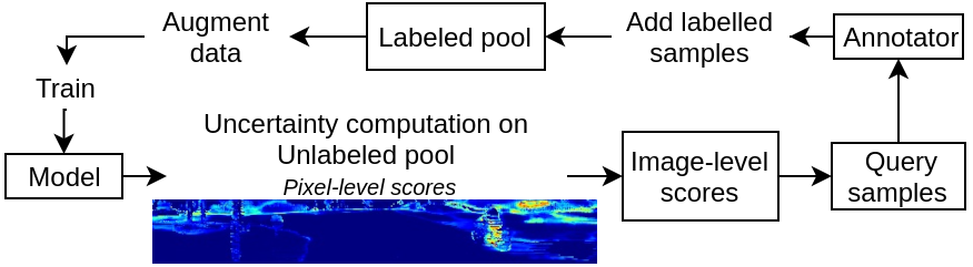
Figure 1: Global flow of active learning on range images from point clouds using uncertainty methods.

Rangenet++ architectures by authors [Milioto et al., 2019] use range image based spherical coordinate representations of point clouds to enable the use of 2D-convolution kernels. The relationship between range image and LiDAR coordinates is the following:

$$\begin{pmatrix}u\\ v\end{pmatrix}=\begin{pmatrix}\frac{1}{2}[1-\arctan(y,x)\pi^{-1}]\times w\\ [1-(\arcsin(z\times r^{-1})+{f}_{up})\times{f}^{-1}]\times h\end{pmatrix},$$

where $(u,v)$ are image coordinates, $(h,w)$ the height and width of the desired range image, $f=f_{up}+f_{down}$, is the vertical $fov$ of the sensor, and $r=\sqrt{x^{2}+y^{2}+z^{2}}$, range measurement of each point. The input to the DNNs used in our study are images of size $W\times H\times 4$, with spatial dimensions $W,H$ determined by the FoV and angular resolution, and 4 channels containing the $x,y$ coordinates of points, $r$ range or depth to each point, $i$ intensity or remission value for each point.

2.2 Bayesian AL: Background

In a supervised learning setup, given a dataset $\mathcal{D}:=\{(\mathbf{x}_{1},y_{1}),(\mathbf{x}_{2},y_{2}),\ldots,(\mathbf{x}_{N},y_{N})\}\subset\mathcal{X}\times\mathcal{Y}$, the DNN is seen as a high dimensional function $f_{\omega}:\mathcal{X}\to\mathcal{Y}$ with model parameters $\omega$. A simple classifier maps each input $x$ to outcomes $y$. A good classifier minimizes the empirical risk $l:\mathcal{Y}\times\mathcal{Y}\to\mathbb{R}$, which is defined with the expectation $R_{\text{emp}}(f):=\mathbb{P}_{X,Y}[Y\neq f(X)]$. The optimal classifier is one that minimizes the above risk. Thus, the classifier’s loss does not explicitly refer to sample-wise uncertainty but rather to obtain a function which makes good predictions on average. We shall use the following terminologies to describe our AL training setup.

1. Labeled dataset $D=\{\left(\mathbf{x}_{i},y_{i}\right)\}_{i=1}^{N}$ where $\mathbf{x}_{i}\in W\times H\times 4$ are range images with 4 input channels, $W,H$ are spatial dimensions, and $y_{i}\in W\times H\times C$ are one-hot encoded ground truth with $C$ classes. The output of the DNN model is distinguished from the ground truth as $\hat{y}_{i}$ with the same dimensions. The 4 channels in our case are x, y, z coordinates and LiDAR intensity channel values.

2. Labeled pool $L\subset D$ and an unlabeled pool $U\subset D$ considered as a data with/without any ground-truth, where at any AL-step $L\cup U=D$, the subsets are disjoint and restore the full dataset.

3. Query size $B$, also called a budget, to fix the number of unlabeled samples selected for labeling

4. Acquisition function, known as heuristic, providing a score for each pixel given the output $\hat{y}_{i}$ of the DNN model, $f:\mathbb{R}^{W\times H\times C}\to\mathbb{R}^{W\times H}$

5. Including the usage of MC iterations where the output of the DNN model could provide several outputs given the same model and input, $\hat{y}_{i}\in W\times H\times C\times T$ where $T$ refers to the number of MC iterations.

6. Subset model $f_{L}$ is the model trained on labeled subset $L$

7. Aggregation function $a:\mathbb{R}^{W\times H\times C\times T}\to\mathbb{R}^{+}$ is a function that aggregates heuristic scores across all pixels in the input image into a positive scalar value, which is used to rank samples in the unlabeled pool.

Heuristic functions are transformations over the model output probabilities $p(y|x)$ that define uncertainty-based metrics to rank and select informative examples from the unlabeled pool at each AL-step. In our previous study [Duong. et al., 2022] we have identified BALD to be a robust heuristic function [Houlsby et al., 2011]. It selects samples maximizing information gain between the predictions from model parameters, using MC Iterations.

2.3 Data augmentations on range images

We apply DA directly on the range image projection. We apply the same transformations as in our previous study [Duong. et al., 2022], we repeat images of the data augmentation here to visually demonstrate them, in figure 2.

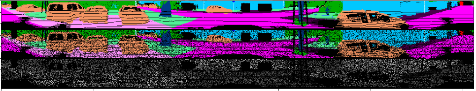
(a) Random dropout mask

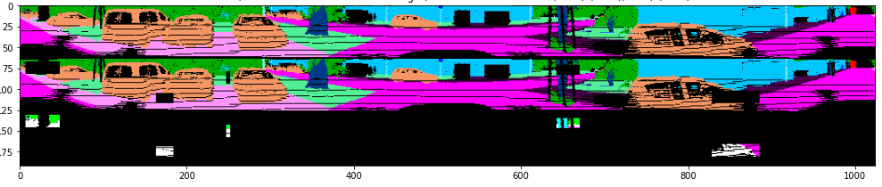
(b) CoarseDropout of Albumentations library

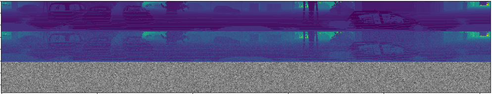
(c) Gaussian noise applied on depth channel

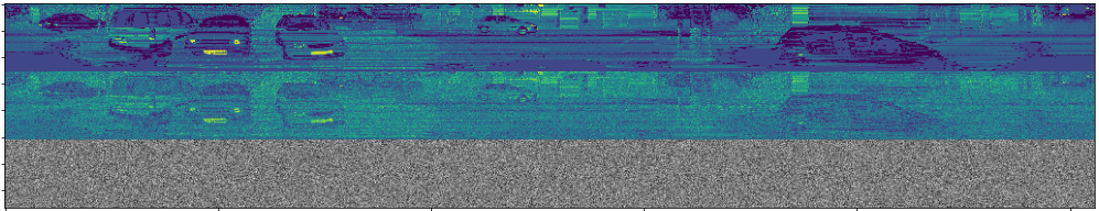
(d) Gaussian noise applied on remission channel

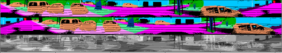
(e) Random cyclic shift range image

(f) Instance Cut Paste

Figure 2: Before and after applying transformations on Semantic-KITTI. Each image corresponds to a sample such that inner images, from top to bottom, are before and after applying transformations, and the error between them. a, b, c, d are directly used or customized based on Albumentations library [Buslaev et al., 2020]

2.4 AL Evaluation metrics

To evaluate the performance of our experiments we are using the following metrics:

• The Mean Intersection over Union (mIoU) [Song et al., 2016]: $\frac{1}{C}\sum^{C}_{c=1}IoU_{c}$

• Labeling efficiency: Authors [Beck et al., 2021] use the labeling efficiency (LE) to compare the amount of data needed among different sampling techniques with respect to a baseline. In our experiments, instead of accuracy, we use mIoU as the performance metric. Given a specific value of mIoU, the labeling efficiency is the ratio between the number of labeled range images, acquired by the baseline sampling and the other sampling techniques.

  $$\text{LE}=\frac{n_{\text{labeled}\_\text{others}}(\text{mIoU}=a)}{n_{\text{labeled}\_\text{baseline}}(\text{mIoU}=a)}$$ (1)

  The baseline method is usually the random heuristic.

3 Experimental Setup

In this study we have evaluated the performance of AL based sampling of a large scale LiDAR dataset Semantic-KITTI. As in [Duong. et al., 2022] we follow a Bayesian AL loop using MC Dropout. The heuristic computes uncertainty scores for each pixel. To obtain the final score per range image, we use sum as an aggregation function to combine all pixel-wise scores of an image into a single score. At each AL step, the unlabeled pool is ranked w.r.t the aggregated score. A new query of samples limited to the budget size is selected from the ranked unlabeled pool. The total number of AL steps is indirectly defined by budget size, $n_{AL}=\left|D\right|/B$

In this study we evaluated BALD [Houlsby et al., 2011] heuristic, while applying it with and without DA applied during training time. As mentioned in Table I, we only use 16000 randomly chosen samples from Semantic-KITTI over the 23201 samples available. At each training step, we reset model weights to avoid biases in the predictions, as proven by [Beck et al., 2021].

Data related parameters			AL Hyper parameters
Range image resolution	Total pool size	Test pool size	Init set size	Budget	MC Dropout	AL steps	Aggregation
1024x64	6000	2000	240	240	0.2	25	sum
Range image resolution	Total pool size	Test pool size	Init set size	Budget	MC Dropout	AL steps	Aggregation
1024x64	16241	6960	1041	800	0.2	20	sum
Hyper parameters for each AL step
Max train iterations	Learning rate (LR)	LR decay	Weight decay	Batch size	Early stopping
					Evaluation period	Metric	Patience
100000	0.01	0.99	0.0001	16	500	train mIoU	15

TABLE I: Active learning (AL) parameter setup (first line for [Duong. et al., 2022] result).

We evaluate LE mIoU as our metric on the test set of 6960 samples. For quicker training, we use early stopping based on the stability of training mIoU over $\textit{patience}*\textit{evaluation}\_\textit{period}$ iterations.

3.1 Analysis of results

The figure 3, demonstrates all the trainings performed on the full Semantic-KITTI dataset. The models SalsaNext (SN) and SqueezeSegV2 (SSV2) were chosen to be evaluated. Both models use rangenet based representations as mentioned earlier. The SSV2 model was trained with and without data augmentation, using a baseline random sampler, the model was also evaluated with BALD heuristic function. SN model was mainly evaluated in the AL framework using data augmentation and with BALD.

The goals here have been to compare the effect of:

• Data augmentation on the label efficiency over a large dataset.

• Difference in model capacity (SN with 6.7M parameters vs SSV2 with 1M parameters) .

• Difference in performance of random sampler vs the BALD heuristic.

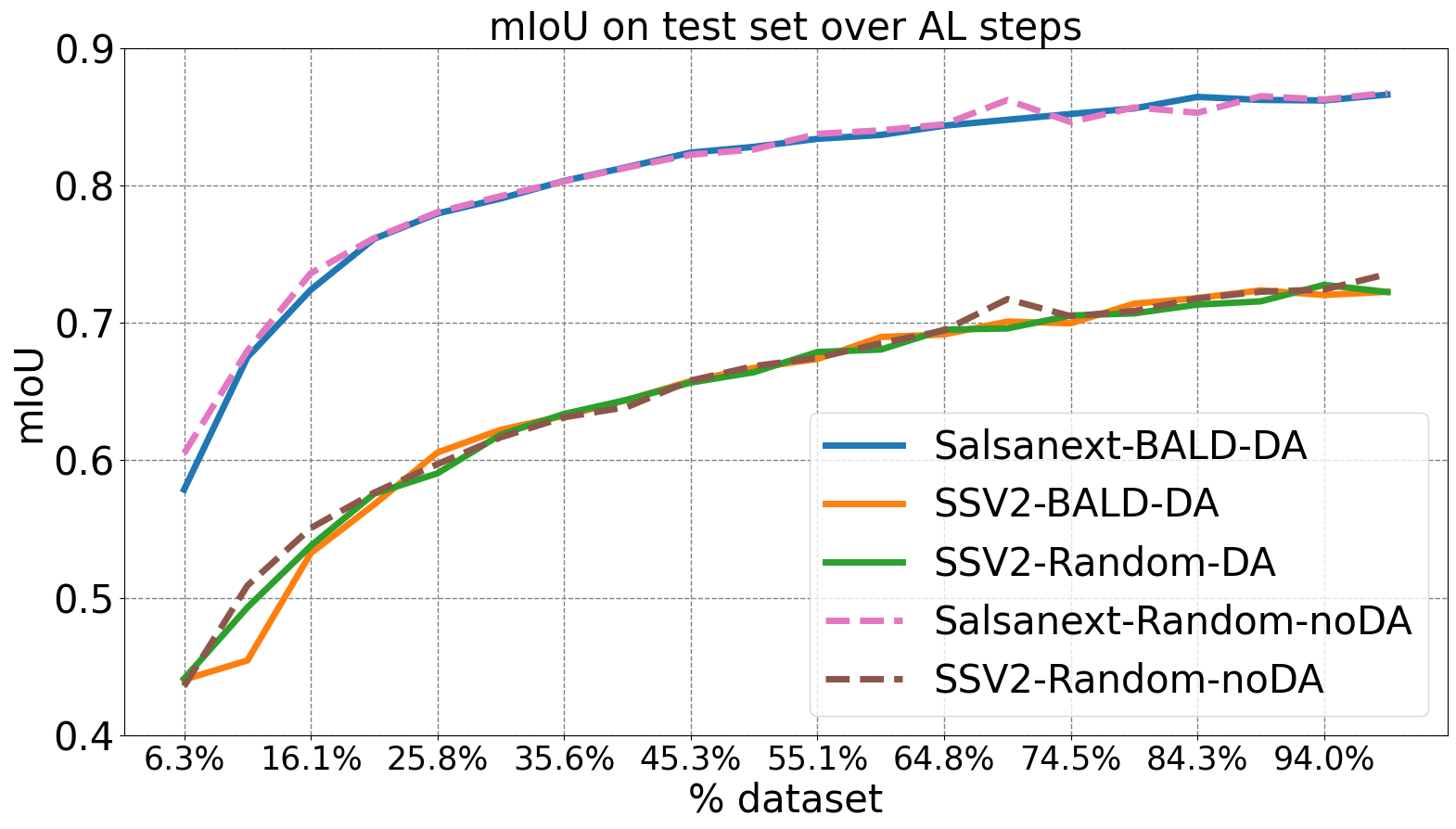
Figure 3: Mean IoU vs dataset size (in percentage) using random and BALD heuristic based samplers under the effect of data augmentation.

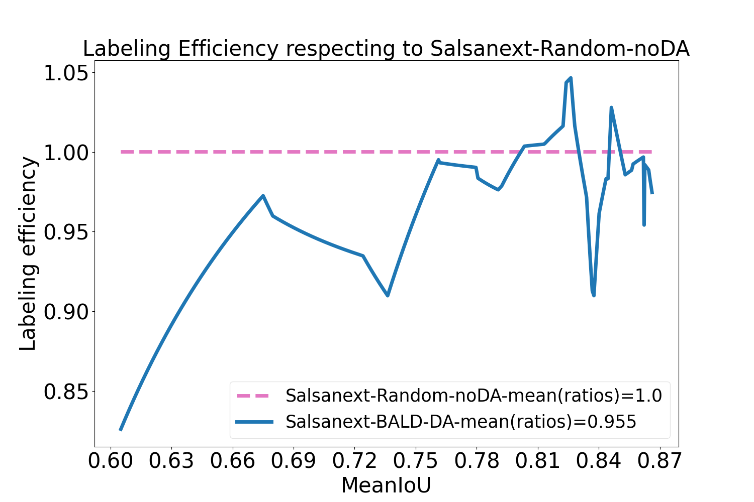
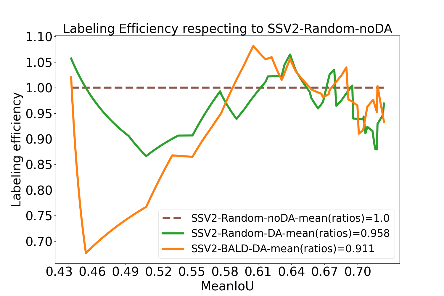
Figure 4: SalsaNext & SSV2 models evaluated w.r.t the Random sampling baseline. The plots demonstrate the label efficiency.

3.2 Class based learning efficiency

In this section we study the variation of ClassIoU for all classes in the Semantic-KITTI dataset. Along with this we also study the variation from mIoU of the fully supervised (FS) model, expressed by:

$$\Delta cIOU[i]=cIoU[i]-mIoU_{\text{FS}}$$ (2)

where $i$ is the index of the active learning loop (or the perception of dataset). This score basically subtracts the mean performance away from the class IoU scores to demonstrate deviations from the mean. The objective of such a measure is to demonstrate the rate at which each class IoU reaches its maximum contribution.

The $\Delta cIOU[i]$ score represents the deviation of the class IoU from the model’s full supervised mean performance. When this deviation is positive and large, these represent classes that have been learnt efficiently at the AL-Step i, while negative scores represent classes that have been learnt poorly. This score enables us to determine visually when each class reaches its maximum performance and decide when any incremental addition of samples would have little impact on the final cIoU.

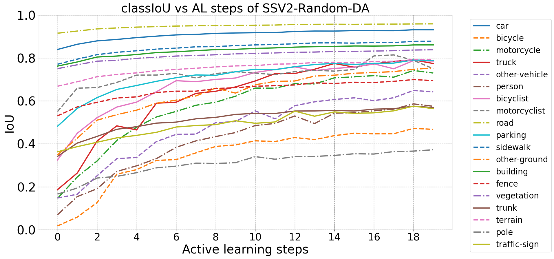
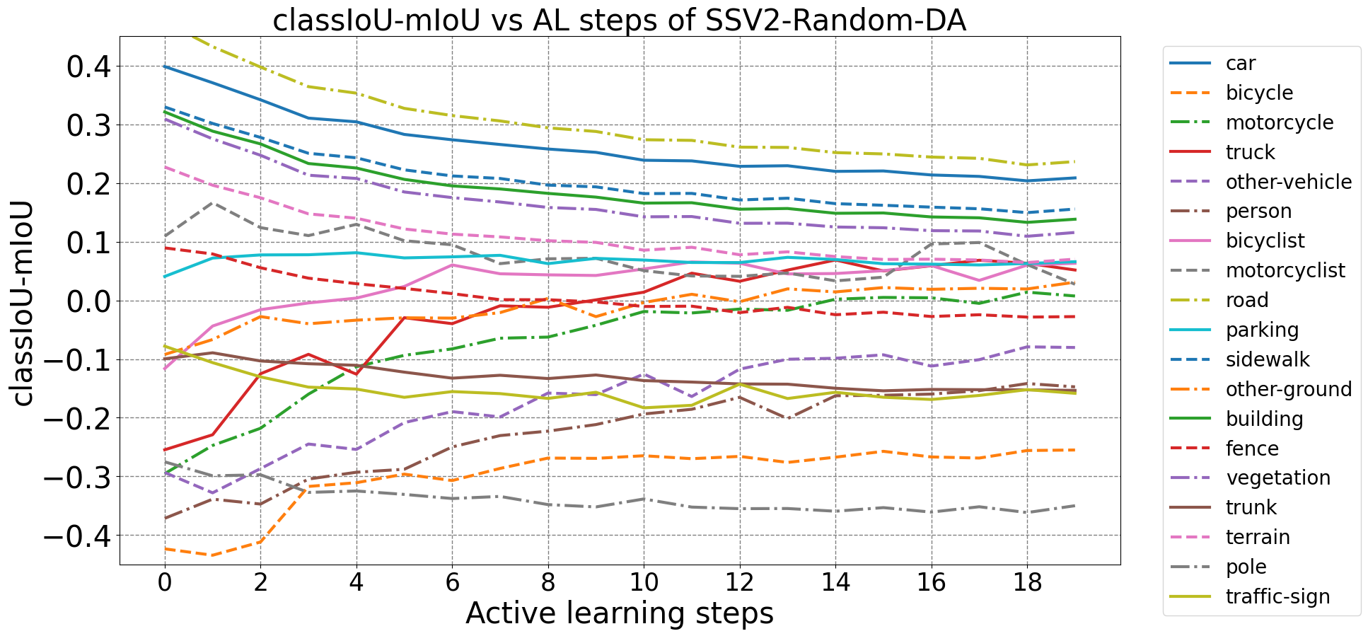
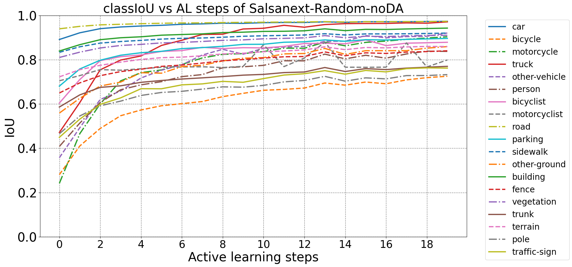
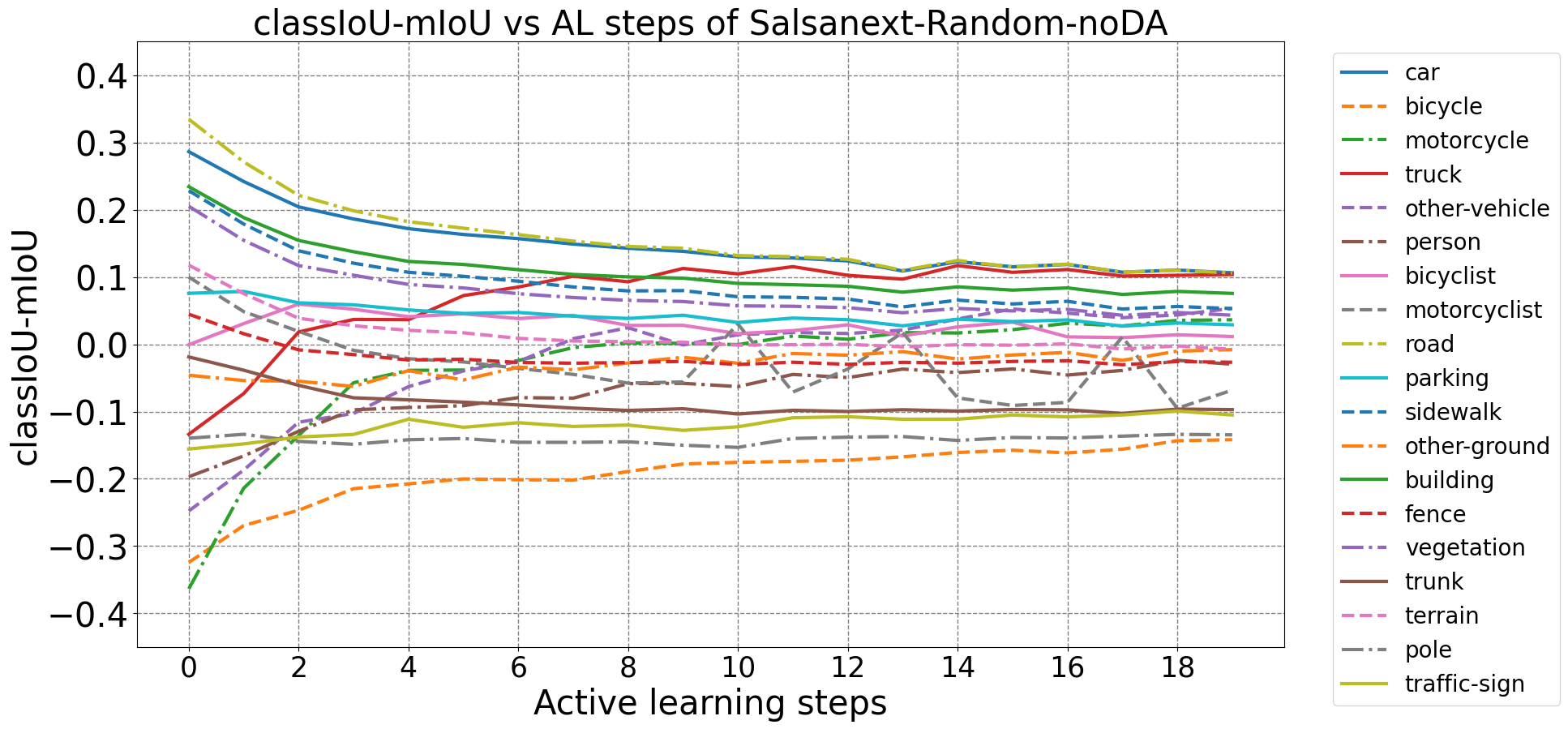
Figure 5: Top Left: Class IoU for SSV2 model Top Right: Deviation from mean IoU from equation 2. Bottom, the same for the SalsaNext model.

Class-frequency and ClassIoU: In figure 5 we observe that several majority classes like ROAD, TERRAIN, BUILDING and VEGETATION do not demonstrate any large change in their IoUs after the 6th AL step, while classes such as BICYCLE, POLE, PERSON and OTHER VEHICLE are the slowest to learn their maximum performance. The majority classes produce a positive deviation from mIoU while the least frequent classes produce a negative deviation from mIoU.

DA effect on ClassIoU: In figure 6 we plot the $\Delta cIoU[i]$ scores to demonstrate how fast different classes are learnt over the AL loop (different subset sizes of the full dataset). With this plot we would like to observe the change in sample complexity for each class with and without data augmentations using baseline random sampling.

Model complexity on ClassIoU: We evaluate two models on the Semantic-KITTI dataset: SSV2 model vs SalsaNext model. We compare the performances of these models in terms of how fast they learn different classes, see figure 7. We observe that majority of classes have had a large jump within the first 3-4 AL steps for the SalsaNext model, demonstrating how model capacity plays an important role in the sample complexity of learning certain classes.

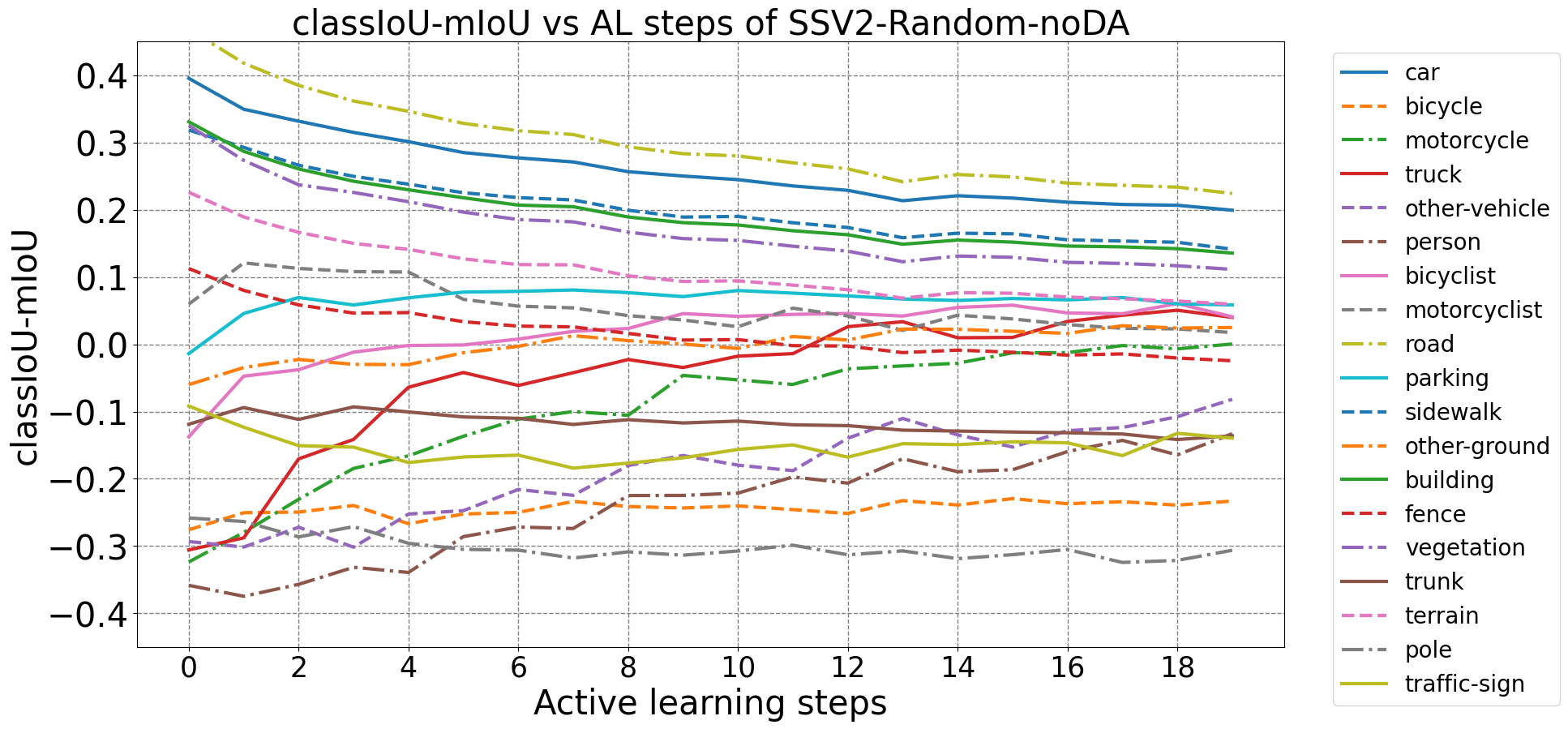
Figure 6: Deviation of Class IoU from mIoU for the SSV2 model: with and without data augmentation applied.

Figure 7: Deviation of ClassIoU from mIoU comparison: Between SSV2 and SN models.

3.3 Dataset size growth: 1/4 Semantic-KITTI vs full Semantic-KITTI

In our previous study on Semantic-KITTI [Duong. et al., 2022] we have evaluated the performance of AL methods while applying data augmentation on 1/4th subset of the Semantic-KITTI dataset. As expected, DA sampled harder samples by eliminating similar samples learnt by invariance. That is to say, models trained with DA are prone to select samples different from the trained samples and their transformations, thus reducing redundancy in the selection.

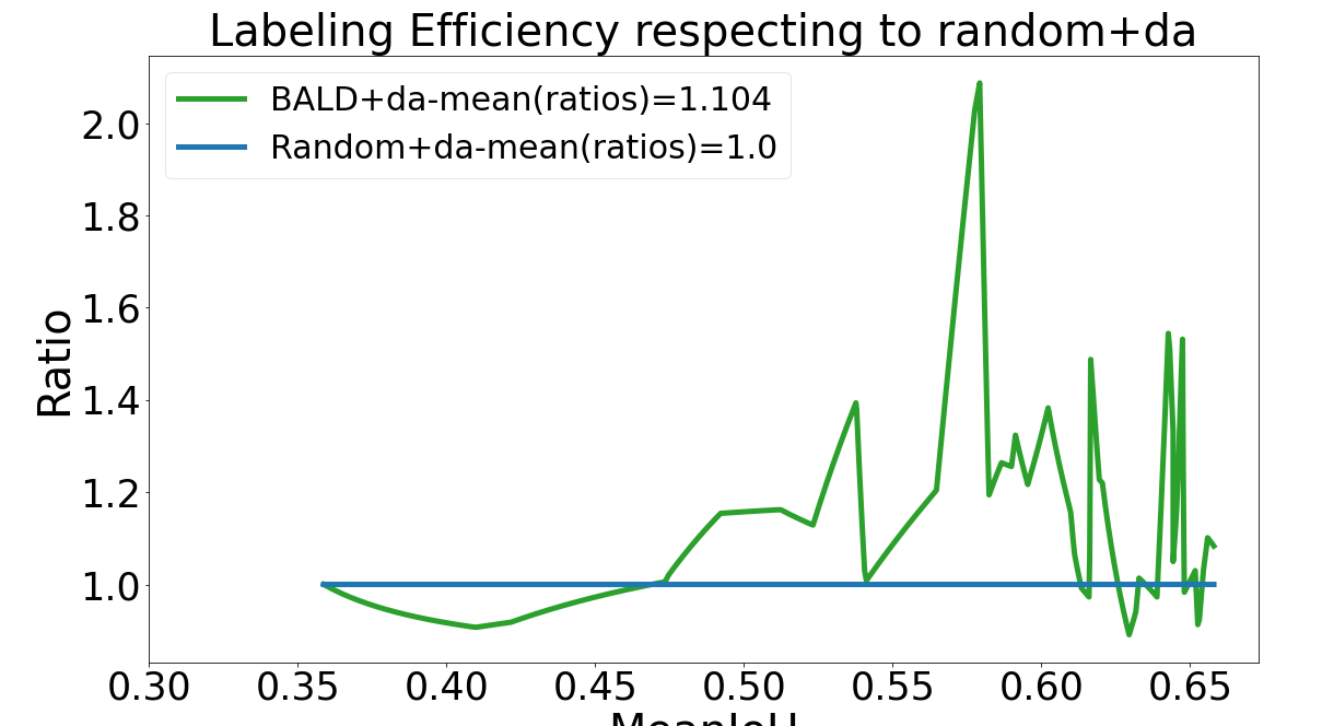
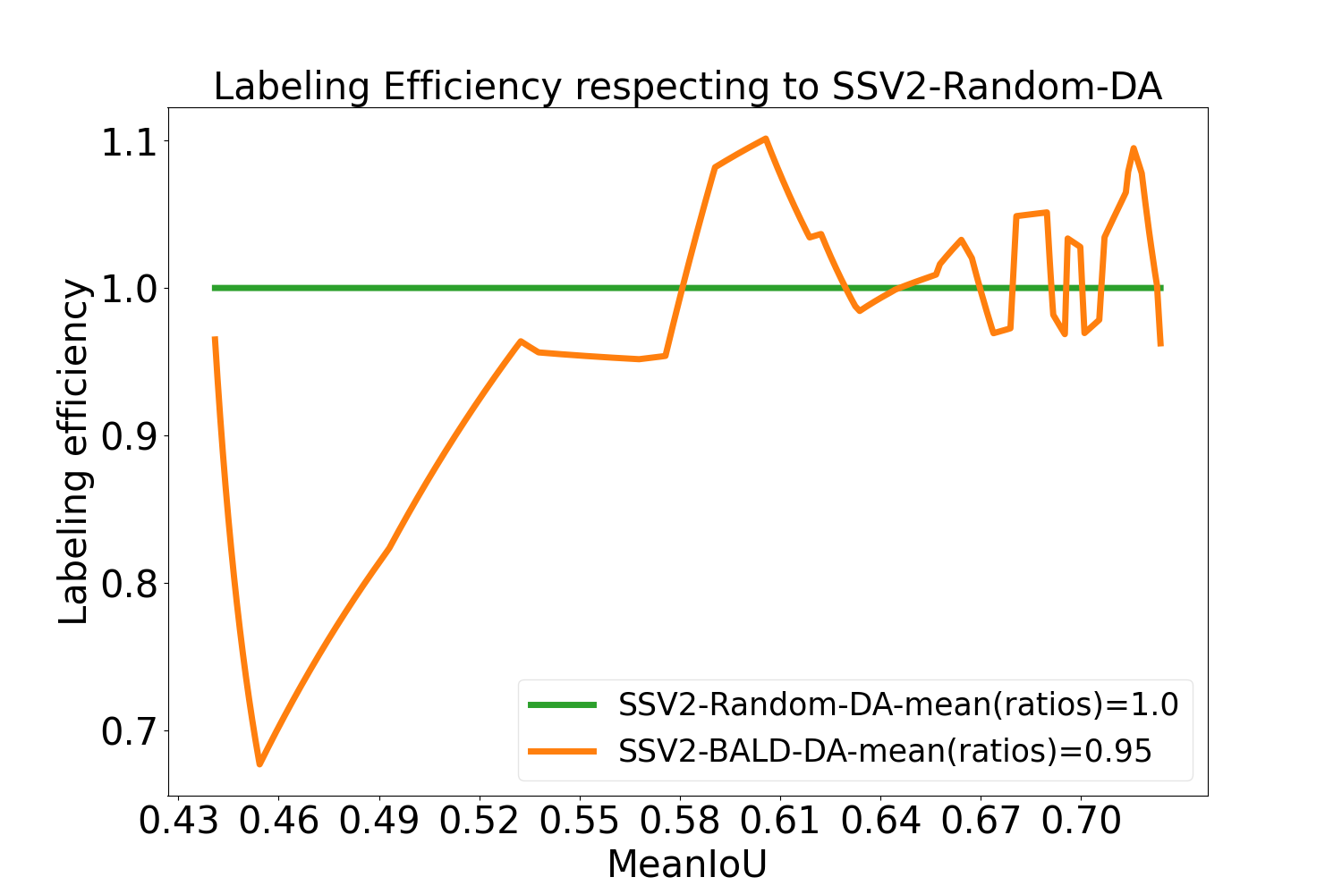
Figure 8: Comparison of the BALD performance. Left: AL training on Semantic-KITTI subset 1/4 from [Duong. et al., 2022], Right: AL training on Semantic-KITTI full dataset from this study. We observe that the two LE are poor in the initial steps, with subsequent increases in the future AL steps.

On the other hand, although DA significantly reduce redundancy in 1/4 Semantic-KITTI experiments, there is almost no increment in the gain by DA in full Semantic-KITTI experiments. This can be seen in figure 8 and could be mainly attributed to the following reasons (we hypothesize):

1. Larger dataset includes larger amount of near similar or redundant samples, but all standalone uncertainty-based methods still encounter the problem of high-score similar samples. Semantic-KITTI is a sequential dataset and thus contain similar scans due to temporal correlation. Thus random sampling breaks this redundancy, while methods like BALD are unable to do so due to the above said reasons. Potential solutions for this problem are mentioned in future work and challenges section below.

2. The gain by DA is getting smaller as dataset size increases because some augmented samples can be found in larger dataset (when dataset is getting larger) or test domain.

3. From the hypothesis, uncorrelated-to-real-world DA can increase uncertainty in predictions of unnecessary sample points, leading wrong prediction and impractical sampling selection.

3.4 t-SNE problem analysis

t-SNE [van der Maaten and Hinton, 2008] is a technique used to visualize high-dimensional data in low-dimensional spaces such as 2D or 3D by minimizing Kullback-Leibler divergence between the low-dimensional distribution and the high-dimensional distribution.

To visualize whether DA is relevant for Semantic-KITTI, we use t-SNE to reduce score images of labeled and DA (labeled) at AL step 0 of Semantic-KITTI/4’s to 2D vector and plot on 2D axes (fig 9). The samples located in regions with dense red color are out-of-training-set-distribution candidates at AL step 0. Visualization of the candidates is in fig 10.

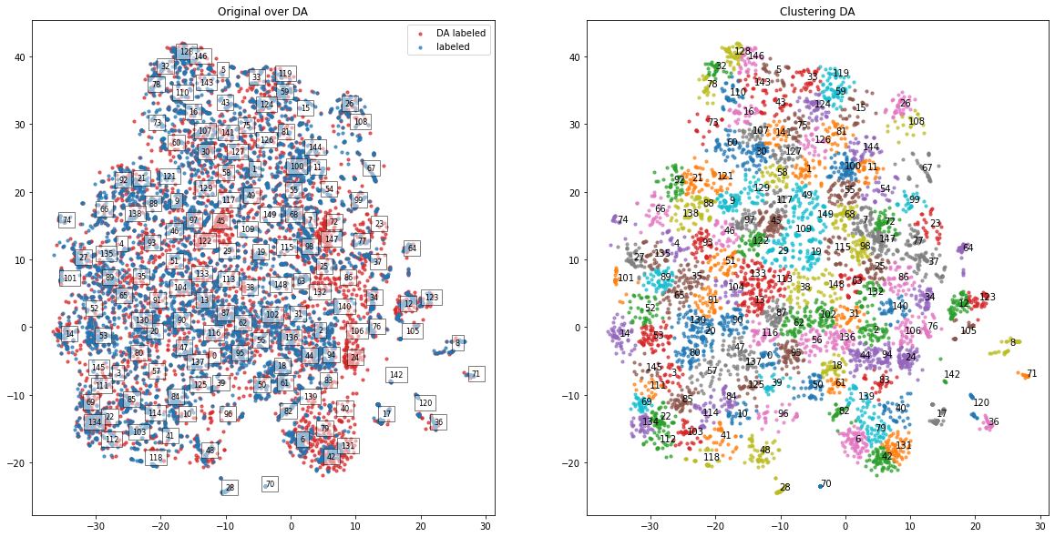
Figure 9: Left image is a t-SNE visualization of labeled and DA(labeled) at step 0. Right image is t-SNE visualization of DA(labeled) clustering region by K-means

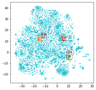
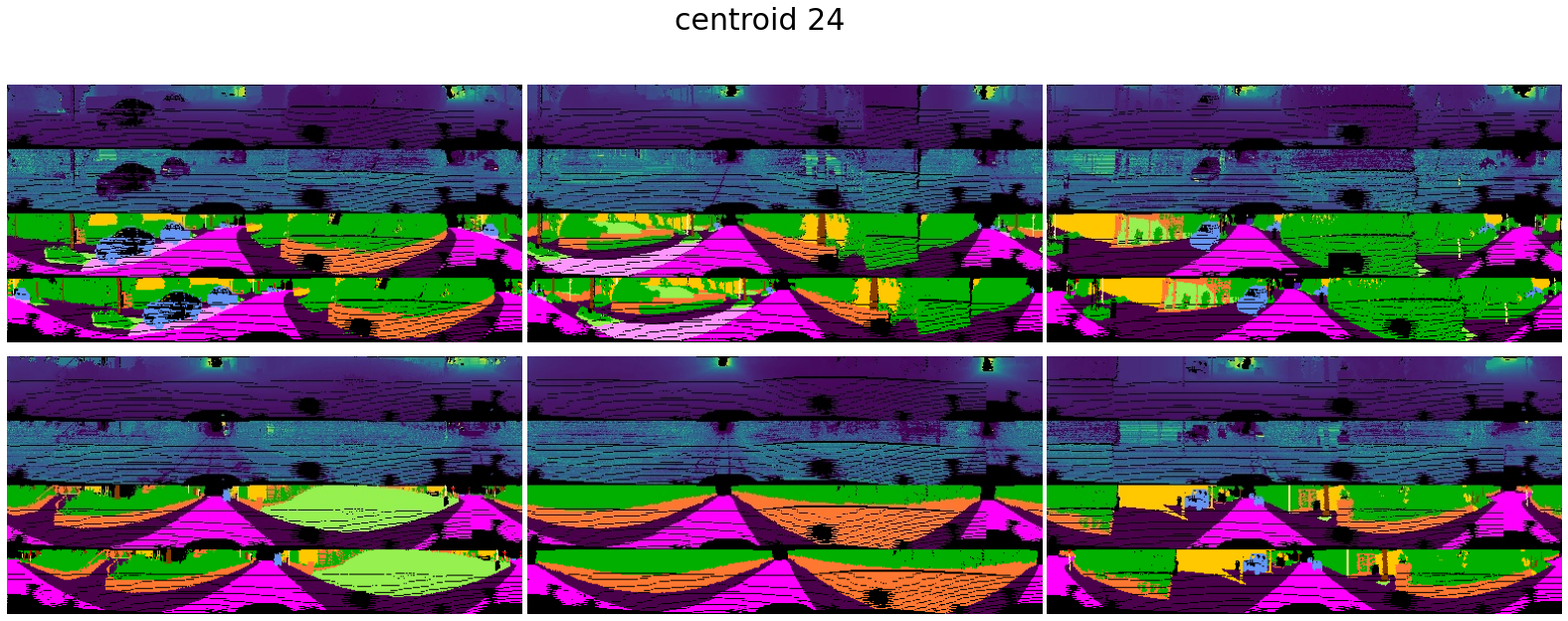
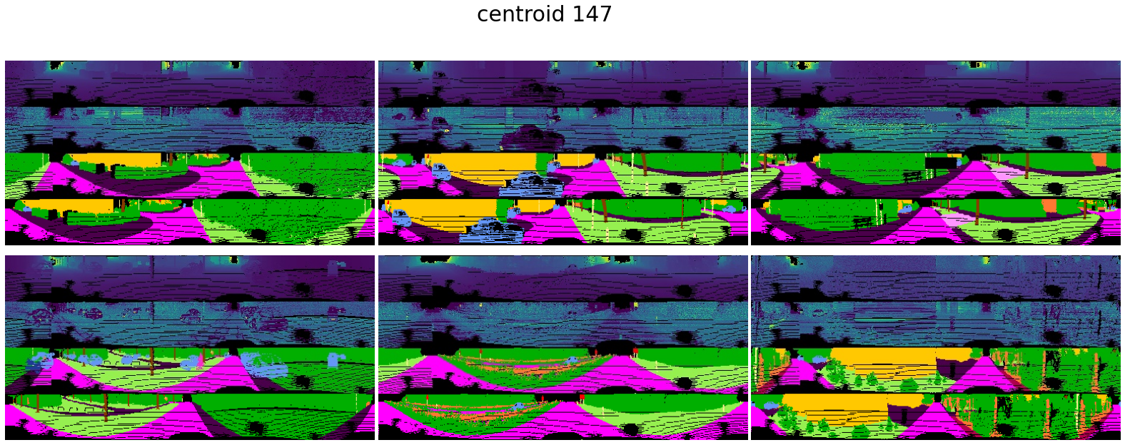
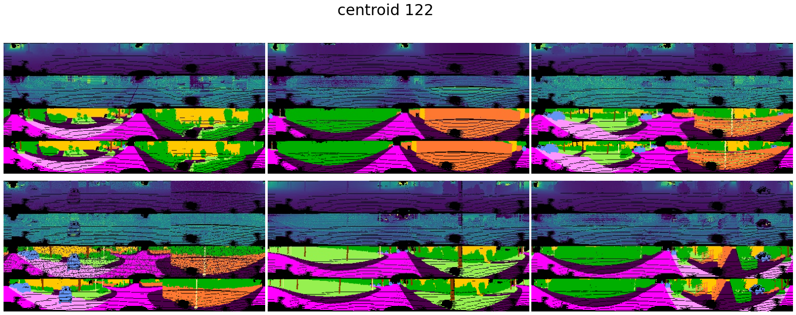
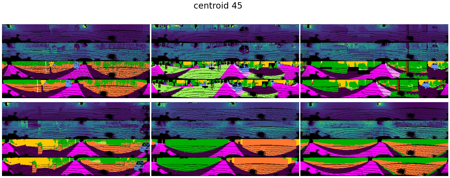
Figure 10: Visualization of samples deviating from dataset distribution.

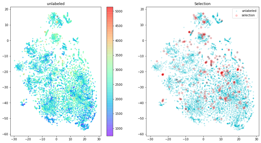
Figure 11: Left image is a t-SNE visualization of unlabeled pool at step 0, whose colors are corresponding to heuristic scores. Right image is the t-SNE visualization of selected samples and unlabeled pool.

In the figure 11, deep red spots show that there are a lot of selected high-score samples concentrated in the same location.

4 Conclusion

Core subset extraction/dataset distillation experiments were carried out on Semantic-KITTI dataset using SalsaNext and SSV2 models. The results of data augmentation and BALD heuristic were limited and did not perform any better than a random sampling method, the first baseline in active learning methods. These limited improvements are an important observation for active learning benchmarks, even though they constitute in marginal gains, and aids further studies to focus on other ways to improve labeling efficiency. Active learning strategies struggle with large-scale datasets such as point clouds in the real-world scenario.

1. Data augmentation’s have a strong effect on the quality of the heuristic function. It is thus key to evaluate data augmentation schemes that are dataset dependant, especially when unlabeled pool is just a small subset of target domain. Inappropriate or overwhelming augmentation can cause out-of-distribution, reducing model bias to target domain. [Fawzi et al., 2016] propose an adaptive data augmentation algorithm for image classification, which looks for a small transform maximizing the loss on that transformed sample.

2. The final aggregation score in an active learning framework is a crucial choice. Aggregation is required when working on detection or segmentation tasks, while most AL study has been focused on classification. Here are a few choices of aggregation functions and how they affect the final ranking of images from which to sample:

   • Sum of all scores: select a sample having a balance of high score and high number of elements.

   • Average of all scores: select a sample having a high score comparable to the others regardless of the number of elements within a sample.

   • Max of all scores: select a sample having the highest element scores of all samples, targeting noises.

   • Weighted average of all scores: similar to average but focus on the given weights. The class weights can be inverse-frequency class weights or customized based on the use case to prioritize the selection for certain classes.

   It is noted that for our proposed method, sum and average eventually yield the same rankings because the number of pixels for range images are constant.

3. Another key issue in industrial datasets is the filtering or exclusion of corrupted or outlier images/point clouds from the AL loop. [Chitta et al., 2019] show that removing top highest uncertain samples as outliers improves model performances.

4. To avoid selection of similar high-score samples and to reduce the sensitivity and bias of the model when training on a small dataset, a potential strategy can be an integration of diversity. Some hybrid methods, such as [Sener and Savarese, 2018] [Kirsch et al., 2019] [Ash et al., 2020] [Yuan et al., 2022], are shown to have more competitive results comparing to standalone uncertainty-based methods for datasets containing high rate of redundancy, but their computations are often costly for large scale point clouds datasets. Another strategy is using temporal information to sample [Aghdam et al., 2019] before or after uncertainty computation. Although it has low computation cost, it cannot ensure the dissimilarity among different samples.

5. According to authors [Chitta et al., 2019] [Pop and Fulop, 2018], MC Dropout is observed to lack of diversity for uncertainty estimation. To address this problem, [Chitta et al., 2019] [Bengar et al., 2019] use multiple checkpoints during training epochs from different random seeds.

6. Pool-based AL might not be a proper AL strategy in real-world scenario for large scale datasets because of unlimited instances streamed sequentially, but limited at any given time. Due to memory limitation, it is impossible to store or re-process all past instances. In this case, stream-based methods are more pertinent by querying annotator for each sample coming from the stream. Although this type of query is often computationally inexpensive, the selected samples are not as informative as the ones selected by pool-based AL due to the lack of exploitation underlying distribution of datasets.

Acknowledgements This work was granted access to HPC resources of [TGCC/CINES/IDRIS] under the allocation 2021- [AD011012836] made by GENCI (Grand Equipement National de Calcul Intensif). It is also part of the Deep Learning Segmentation (DLS) project financed by ADEME.

References

- [Aghdam et al., 2019] Aghdam, H. H., Gonzalez-Garcia, A., van de Weijer, J., and López, A. M. (2019). Active learning for deep detection neural networks.
- [Anselmi et al., 2016] Anselmi, F., Rosasco, L., and Poggio, T. (2016). On invariance and selectivity in representation learning. Information and Inference: A Journal of the IMA, 5(2):134–158.
- [Ash et al., 2020] Ash, J. T., Zhang, C., Krishnamurthy, A., Langford, J., and Agarwal, A. (2020). Deep batch active learning by diverse, uncertain gradient lower bounds.
- [Atighehchian et al., 2019] Atighehchian, P., Branchaud-Charron, F., Freyberg, J., Pardinas, R., and Schell, L. (2019). Baal, a bayesian active learning library. https://github.com/ElementAI/baal/.
- [Atighehchian et al., 2020] Atighehchian, P., Branchaud-Charron, F., and Lacoste, A. (2020). Bayesian active learning for production, a systematic study and a reusable library.
- [Beck et al., 2021] Beck, N., Sivasubramanian, D., Dani, A., Ramakrishnan, G., and Iyer, R. (2021). Effective evaluation of deep active learning on image classification tasks.
- [Behley et al., 2019] Behley, J., Garbade, M., Milioto, A., Quenzel, J., Behnke, S., Stachniss, C., and Gall, J. (2019). Semantickitti: A dataset for semantic scene understanding of lidar sequences.
- [Bengar et al., 2019] Bengar, J. Z., Gonzalez-Garcia, A., Villalonga, G., Raducanu, B., Aghdam, H. H., Mozerov, M., Lopez, A. M., and van de Weijer, J. (2019). Temporal coherence for active learning in videos.
- [Birodkar et al., 2019] Birodkar, V., Mobahi, H., and Bengio, S. (2019). Semantic redundancies in image-classification datasets: The 10don’t need.
- [Brostow et al., 2009] Brostow, G. J., Fauqueur, J., and Cipolla, R. (2009). Semantic object classes in video: A high-definition ground truth database. Pattern Recognit. Lett., 30:88–97.
- [Buslaev et al., 2020] Buslaev, A., Iglovikov, V. I., Khvedchenya, E., Parinov, A., Druzhinin, M., and Kalinin, A. A. (2020). Albumentations: Fast and flexible image augmentations. Information, 11(2).
- [Caesar et al., 2020] Caesar, H., Bankiti, V., Lang, A. H., Vora, S., Liong, V. E., Xu, Q., Krishnan, A., Pan, Y., Baldan, G., and Beijbom, O. (2020). nuscenes: A multimodal dataset for autonomous driving.
- [Chitta et al., 2019] Chitta, K., Alvarez, J. M., Haussmann, E., and Farabet, C. (2019). Training data subset search with ensemble active learning. arXiv preprint arXiv:1905.12737.
- [Cordts et al., 2016] Cordts, M., Omran, M., Ramos, S., Rehfeld, T., Enzweiler, M., Benenson, R., Franke, U., Roth, S., and Schiele, B. (2016). The cityscapes dataset for semantic urban scene understanding.
- [Cortinhal et al., 2020] Cortinhal, T., Tzelepis, G., and Aksoy, E. E. (2020). Salsanext: Fast, uncertainty-aware semantic segmentation of lidar point clouds for autonomous driving.
- [Duong. et al., 2022] Duong., A., Almin., A., Lemarié., L., and Kiran., B. (2022). Lidar dataset distillation within bayesian active learning framework understanding the effect of data augmentation. In Proceedings of the 17th International Joint Conference on Computer Vision, Imaging and Computer Graphics Theory and Applications - Volume 4: VISAPP,, pages 159–167. INSTICC, SciTePress.
- [Fawzi et al., 2016] Fawzi, A., Samulowitz, H., Turaga, D., and Frossard, P. (2016). Adaptive data augmentation for image classification. In 2016 IEEE International Conference on Image Processing (ICIP), pages 3688–3692.
- [Gal and Ghahramani, 2016] Gal, Y. and Ghahramani, Z. (2016). Dropout as a bayesian approximation: Representing model uncertainty in deep learning.
- [Gal et al., 2017] Gal, Y., Islam, R., and Ghahramani, Z. (2017). Deep bayesian active learning with image data.
- [Golestaneh and Kitani, 2020] Golestaneh, S. A. and Kitani, K. M. (2020). Importance of self-consistency in active learning for semantic segmentation.
- [Hong et al., 2020] Hong, S., Ha, H., Kim, J., and Choi, M.-K. (2020). Deep active learning with augmentation-based consistency estimation. arXiv preprint arXiv:2011.02666.
- [Houlsby et al., 2011] Houlsby, N., Huszár, F., Ghahramani, Z., and Lengyel, M. (2011). Bayesian active learning for classification and preference learning.
- [Kendall and Gal, 2017] Kendall, A. and Gal, Y. (2017). What uncertainties do we need in bayesian deep learning for computer vision?
- [Kirsch et al., 2019] Kirsch, A., van Amersfoort, J., and Gal, Y. (2019). Batchbald: Efficient and diverse batch acquisition for deep bayesian active learning.
- [Milioto et al., 2019] Milioto, A., Vizzo, I., Behley, J., and Stachniss, C. (2019). Rangenet++: Fast and accurate lidar semantic segmentation. In 2019 IEEE/RSJ International Conference on Intelligent Robots and Systems (IROS), pages 4213–4220. IEEE.
- [Pop and Fulop, 2018] Pop, R. and Fulop, P. (2018). Deep ensemble bayesian active learning : Addressing the mode collapse issue in monte carlo dropout via ensembles.
- [Sener and Savarese, 2018] Sener, O. and Savarese, S. (2018). Active learning for convolutional neural networks: A core-set approach.
- [Settles, 2009] Settles, B. (2009). Active learning literature survey.
- [Song et al., 2016] Song, S., Yu, F., Zeng, A., Chang, A. X., Savva, M., and Funkhouser, T. (2016). Semantic scene completion from a single depth image.
- [Uricár et al., 2019] Uricár, M., Hurych, D., Krizek, P., and Yogamani, S. (2019). Challenges in designing datasets and validation for autonomous driving. arXiv preprint arXiv:1901.09270.
- [van der Maaten and Hinton, 2008] van der Maaten, L. and Hinton, G. (2008). Viualizing data using t-sne. Journal of Machine Learning Research, 9:2579–2605.
- [Wu et al., 2018] Wu, B., Zhou, X., Zhao, S., Yue, X., and Keutzer, K. (2018). Squeezesegv2: Improved model structure and unsupervised domain adaptation for road-object segmentation from a lidar point cloud.
- [Wu et al., 2021] Wu, T.-H., Liu, Y.-C., Huang, Y.-K., Lee, H.-Y., Su, H.-T., Huang, P.-C., and Hsu, W. H. (2021). Redal: Region-based and diversity-aware active learning for point cloud semantic segmentation.
- [Yuan et al., 2022] Yuan, S., Sun, X., Kim, H., Yu, S., and Tomasi, C. (2022). Optical flow training under limited label budget via active learning.