Rectification and Nonlinear Hall effect by Fluctuating Finite-momentum Cooper Pairs

Abstract

Nonreciprocal charge transport is attracting much attention as a novel probe and functionality of noncentrosymmetric superconductors. In this work, we show that both the longitudinal and transverse nonlinear paraconductivity is hugely enhanced in helical superconductors under moderate and high magnetic fields, which can be observed by second-harmonic resistance measurements. The discussion is based on the generalized formulation of nonlinear paraconductivity in combination with the microscopically determined Ginzburg-Landau coefficients. The enhanced nonreciprocal transport would be observable even with the cyclotron motion of fluctuating Cooper pairs, which is elucidated with a Kubo-type formula of the nonlinear paraconductivity. Nonreciprocal charge transport in the fluctuation regime is thereby established as a promising probe of helical superconductivity regardless of the sample dimensionality. Implications on the other finite-momentum superconducting states are briefly discussed.

Introduction. — Nonreciprocal charge transport (NCT) is attracting much attention as the novel functionality of noncentrosymmetric materials [1, 2, 3, 4, 5, 6, 7, 8, 9, 10, 11, 12, 13, 14, 15, 16, 17, 18, 19, 20, 21, 22, 23, 24, 25, 26, 27, 28, 29, 30, 31, 32, 33, 34, 35]. An example is a diode-like material property known as magnetochiral anisotropy (MCA), which refers to directional resistance, or rectification, linear in the magnetic field and has been observed in a variety of materials [3, 4, 5, 6, 7, 8, 9]. Unidirectional transport even with zero and finite resistance has also been realized, namely the superconducting diode effect (SDE) [10, 11, 12, 13, 14, 15, 16, 17, 18, 19, 20, 21, 22]. The nonlinear Hall effect (NHE) is another hot topic [24, 25, 26, 27, 28, 29], by which a finite transverse resistance can be produced in time-reversal symmetric materials. These findings pave the way for next-generation devices such as antennas [9], energy-saving rectifiers [17, 18], and broad-band photodetectors [30, 31]. Furthermore, NCT would highly contribute to fundamental physics as versatile electrical probes of inversion-symmetry breaking, applicable even under extreme conditions including high pressure and magnetic fields. Thus, NCT phenomena are the hallmarks of modern condensed matter physics.

The development of NCT techniques may shed light on the fascinating phenomena of noncentrosymmetric superconductors that are hardly captured via conventional experiments. Among other things, helical superconductivity [36, 37, 38, 39, 40, 41, 42, 43, 44, 45, 36, 46, 47] is a long-sought-after finite-momentum superconducting state, regardless of its predicted ubiquity under magnetic fields. The pair potential of helical superconductivity has a plain-wave expression known as the Fulde-Ferrell type [48] without the modulation of amplitude. This makes its experimental identification more difficult than the Larkin-Ovchinnikov and pair-density-wave states [49, 50, 51, 52], whose detection has been reported via spatially-resolved techniques in various superconductors [53, 54, 55, 56, 57, 58, 59, 60, 61, 62] including FeSe [57], Sr₂RuO₄ [58], Bi₂Sr₂CaCu₂O_8+δ [59, 60], CsV₃Sb₅ [61], and UTe₂ [62]. Recent theoretical studies [20, 22, 63] have revealed that the characteristic crossover phenomenon of helical superconductivity can be signaled by the sign reversal of SDE, offering a promising probe free of Josephson junctions in contrast to the known methods [41, 64]. Further investigation of NCT would provide us with keys to understanding exotic superconducting states in noncentrosymmetric systems.

The disadvantage of SDE as a probe of helical superconductivity is to require small-width samples to approach the depairing limit [20]. Unfortunately, the candidate helical superconductors are two- or quasi-two-dimensional systems such as heavy-fermion superlattices [65, 66] and thin films of Pb [67] and SrTiO₃ [68]. To study such systems without additional microfabrication, we turn renewed attention to the nonreciprocal paraconductivity, i.e., NCT by fluctuating Cooper pairs. In pioneering works [6, 32, 33], nonreciprocal paraconductivity has been studied focusing on MCA. The theoretical studies not only succeeded in explaining the experiment in MoS₂ [6], but also pointed out that spin-singlet and -triplet mixing of Cooper pairs can be detected [32, 33]. However, their formulation is not applicable in the presence of finite-momentum Cooper pairs and/or nonlinear effects of the magnetic field, leaving helical superconductors out of its scope.

In this Letter, we generalize the previous formulation of nonreciprocal paraconductivity and show that the rectification and NHE in the fluctuation regime are hugely enhanced in helical superconductors under moderate and strong magnetic fields. We also show that the enhanced NCT would still be observable even in the presence of the cyclotron motion of Cooper pairs. Our formulation is applicable to Fulde-Ferrell-type superconducting states in general, while thin-film Larkin-Ovchinnikov superconductors may also be explored by applying symmetry-breaking perturbations.

Notations for NCT. — We begin with introducing the notations for rectification and NHE, which is described by the nonlinear conductivity $j_{i}=\sigma_{1}^{ij}E_{j}+\sigma_{2}^{ijk}E_{j}E_{k}$ or the nonlinear resistivity $E_{i}=\rho^{ij}j_{j}=\rho_{1}^{ij}j_{j}+\rho_{2}^{ijk}j_{j}j_{k}.$ Here, linear and nonlinear resistivity satisfy $\rho_{1}^{ij}=[\sigma_{1}^{-1}]_{ij}$ and

$$\rho_{2}^{ijk}=-[\sigma_{1}^{-1}]_{ia}\sigma_{2}^{abc}[\sigma_{1}^{-1}]_{bj}[\sigma_{1}^{-1}]_{ck}.$$ (1)

The nonlinear resistivity can be observed via the longitudinal and Hall second-harmonic resistance [5],

$$R^{2\omega}_{x,{\rm L}} =\frac{L_{x}j_{x}}{2L_{y}L_{z}}\rho_{2}^{xxx},\quad R^{2\omega}_{x,{\rm H}}=\frac{j_{y}}{2L_{z}}\rho_{2}^{xyy},$$ (2)

under the current density $j_{x}$ and $j_{y}$, respectively. Here we denote the sample diameters by $L_{x},L_{y}$, and $L_{z}$. Note that $\rho_{2}^{xxx}$ gives rise to nonreciprocity in $\rho^{xx}$:

$$\rho^{xx}=\rho_{1}^{xx}(1+\eta^{xxx}j_{x}),\quad\eta^{xxx}\equiv\rho_{2}^{xxx}/\rho_{1}^{xx},$$ (3)

where $1/\eta^{xxx}$ gives a typical current density for nonreciprocity to be visible. The parameter $\eta^{xxx}$ is a natural generalization of the $\gamma$-value for MCA [1, 2], and is used as a quantitative measure of rectification in this paper. We also introduce $\eta^{xyy}\equiv\rho_{2}^{xyy}/\rho_{1}^{xx}$ to compare NHE with rectification, whose ratio to $\eta^{xxx}$ coincides with that of $\rho_{2}^{xyy}$ to $\rho_{2}^{xxx}$.

Near the transition temperature ${T_{\rm c}}$ of superconductors, $\sigma_{1}$ tends to diverge due to the fluctuation of Cooper pairs, which interpolates the finite and vanishing resistance in normal and superconducting states [69]. The conductivity in the normal state and the excess contribution by fluctuation are indicated by the subscripts ‘’${\rm{n}}$” and ‘’${\rm{s}}$”, respectively: $\sigma_{1}=\sigma_{1{\rm{n}}}+\sigma_{1{\rm{s}}}$ and $\sigma_{2}=\sigma_{2{\rm{n}}}+\sigma_{2{\rm{s}}}$. Our purpose is to obtain the paraconductivity contributions $\sigma_{1{\rm{s}}}$ and $\sigma_{2{\rm{s}}}$ and thereby evaluate $\rho^{xxx}$ and $\rho^{xyy}$ in the fluctuation regime of superconductors.

Time-dependent GL theory. — Let us consider a $d$-dimensional superconductor slightly above ${T_{\rm c}}$, with $d=2$ unless otherwise specified. Following Refs. [6, 32, 33], we study the fluctuation of Cooper pairs by using the phenomenological time-dependent GL equation in the momentum space [70],

$$\Gamma_{0}\frac{\partial\psi_{\bm{q}}(t)}{\partial t} =-\alpha_{\bm{q}}\psi_{\bm{q}}(t)+\zeta_{\bm{q}}(t),$$ (4a)

$$\braket{\zeta^{*}_{\bm{q}}(t)\zeta_{\bm{q}^{\prime}}(t^{\prime})} =\frac{2\Gamma_{0}T}{V}\delta(t-t^{\prime})\delta_{\bm{q},\bm{q}^{\prime}},$$ (4b)

with the GL functional $F[\psi]=V\sum_{\bm{q}}\alpha_{\bm{q}}|\psi_{\bm{q}}|^{2}$. The random force $\zeta_{\bm{q}}(t)$ is assumed to be the white noise as in the second line and reproduces $\braket{}{\psi_{\bm{q}}}{{}^{2}}=T/V\alpha_{\bm{q}}$ in equilibrium. The effect of the electric field $\bm{E}$ is introduced by $\alpha_{\bm{q}}\to\alpha_{\bm{q}-2\bm{A}(t)}$ with $\bm{A}(t)=-\bm{E}t$. The excess current density by fluctuating Cooper pairs is evaluated with the formula [6, 71, 70]

$$\bm{j}_{\rm{s}} =\lim_{t\to\infty}-\sum_{\bm{q}}\partial_{\bm{A}}\alpha_{\bm{q}-2\bm{A}(t)}\braket{}{\psi_{\bm{q}}(t)}{{}^{2}}$$ (5)

$$=\frac{4T}{\Gamma_{0}}\int\frac{d^{d}q}{(2\pi)^{d}}\partial_{\bm{q}}\alpha_{\bm{q}}\int^{0}_{-\infty}dt_{1}\,e^{-\frac{2}{\Gamma_{0}}\int^{0}_{t_{1}}dt^{\prime}\,\alpha_{\bm{q}-2\bm{A}(t^{\prime})}}.$$

Within the GL picture, the superconducting transition is triggered by the softening of the mode $\bm{q}=\bm{q}_{0}$ which minimizes $\alpha_{\bm{q}}$. This occurs at $\bm{q}_{0}\neq 0$ in helical superconductivity, in contrast to $\bm{q}_{0}=0$ in conventional superconductors. Note that the modes around $\bm{q}_{0}$ dominantly contribute to transport properties in the vicinity of ${T_{\rm c}}$. Thus, we can expand the GL coefficient in terms of $\delta\bm{q}=\bm{q}-\bm{q}_{0}$,

$$\alpha_{\bm{q}} =\alpha_{\bm{q}_{0}}+\alpha_{2}^{ij}\delta q_{i}\delta q_{j}+\alpha_{3}^{ijk}\delta q_{i}\delta q_{j}\delta q_{k}+O(\delta q^{4})$$ (6)

$$\equiv N_{0}\left(\epsilon+\sum_{i}\xi_{i}^{2}\delta q_{i}^{2}+\bar{\xi}\,{}^{3}\sum_{ijk}\mathcal{A}^{ijk}\delta q_{i}\delta q_{j}\delta q_{k}\right).$$

We defined the reduced temperature $\epsilon\equiv(T-{T_{\rm c}})/T$, GL coherence length $\xi_{i}$, its geometric mean $\bar{\xi}\equiv(\prod_{i=1}^{d}\xi_{i})^{1/d}$, and the dimensionless third-rank tensor ${\mathcal{A}}^{ijk}$, while the overall coefficient $N_{0}\equiv T\frac{\partial}{\partial T}\alpha_{\bm{q}_{0}}$ is related to the density of states. Importantly, cubic anharmonicity ${\mathcal{A}}^{ijk}$ is allowed with $\bm{q}_{0}\neq 0$ and/or without both inversion and time-reversal symmetries. Since $\bm{q}_{0}$ can be traced out from Eq. (5) by shifting the momentum, it is the anharmonicity parameter ${\mathcal{A}}^{ijk}$ that gives rise to the nonreciprocal transport [6, 33].

Nonlinear Paraconductivity. —The GL formula of the fluctuation conductivity can be obtained by plugging Eq. (6) into Eq. (5) and expanding it by $\bm{E}$. We neglect the orbital magnetic field for the time being, while the effect of the Zeeman field can be taken into account. The linear fluctuation conductivity is given by [70, 69, 72]

$$L_{z}\sigma_{1{\rm{s}}}^{ij} =\frac{\tau_{0}T}{2\pi\epsilon}\frac{\xi_{i}^{2}}{\xi_{x}\xi_{y}}\delta_{ij},$$ (7)

to the leading order of $\epsilon$, with the sample thickness $L_{z}$ and $\tau_{0}\equiv\Gamma_{0}/N_{0}>0$. This reproduces $L_{z}\sigma_{1{\rm{s}}}=1/{16\epsilon}$ for the GL relaxation time $\tau_{0}=\pi/8T$ [69], in the absence of anisotropy.

The nonlinear paraconductivity is similarly obtained [70],

$$L_{z}\sigma_{2{\rm{s}}}^{ijk} =\frac{\tau_{0}^{2}T\sqrt{\xi_{x}\xi_{y}}}{4\pi\epsilon^{2}}{\mathcal{A}}^{ijk},$$ (8a)

to the leading order of $$\epsilon O(\epsilon^{-2}) \sigma_{2{\rm{s}}}^{ijk} \sigma_{1{\rm{s}}}^{ij} \mathrm{Im}[\Gamma_{0}] d=1 3$$. This is of as reported previously [6, 32, 33]. Note that allows not only rectification but also NHE. This makes sharp contrast to , whose Hall response requires the out-of-plane orbital magnetic field as well as a generally small parameter originated from the particle-hole asymmetry [69]. Nonlinear paraconductivity for system dimensions and are also obtained as

$$L_{y}L_{z}\sigma_{2{\rm{s}}}^{xxx}=\frac{3\tau_{0}^{2}T\xi_{x}^{2}}{8\epsilon^{5/2}}{\mathcal{A}}^{xxx},\quad\sigma_{2{\rm{s}}}^{ijk}=\frac{\tau_{0}^{2}T}{16\pi\epsilon^{3/2}}{\mathcal{A}}^{ijk},$$ (8b)

respectively, where $L_{y}L_{z}$ is the wire cross-section. We emphasize that the obtained formulas allow us to discuss the nonlinear effect of the Zeeman field $\bm{h}$ and, if any, coexisting time-reversal-breaking orders, in contrast to the previous formulas showing $O(h)$ NCT in specific two-dimensional models [6, 32, 33]. This point is crucial to describe fluctuating finite-momentum Cooper pairs.

To illustrate the formula (8a), we discuss NCT linear in the Zeeman field $\bm{h}$ before studying the nonlinear effects of $\bm{h}$. In this case, ${\mathcal{A}}^{ijk}=O(h)$ can be rewritten in the form of the cubic spin-orbit coupling (SOC) [63],

$${\mathcal{A}}^{ijk}\delta q_{i}\delta q_{j}\delta q_{k}\equiv\bm{h}\cdot\bm{g}_{\mathcal{A}}(\delta\bm{q}).$$ (9)

The effect of $\bm{h}$ on the other coefficients is $O(h^{2})$ and thus is negligible in the low-field region. For the purpose of symmetry considerations, the effective SOC $\bm{g}_{\mathcal{A}}(\delta\bm{q})$ can be identified with the antisymmetric SOC of the system around the Gamma point in the Brilloiun zone [63]. Typical forms of the effective SOC in Rashba, chiral, Ising, and Dresselhaus systems are illustrated with a unit vector $\hat{n}$ in Table 1.

Table 1: Typical forms of $\bm{g}_{\mathcal{A}}(\hat{n})=\bm{g}_{\mathcal{A}}(\delta\bm{q})/\delta q^{3}$ and $\frac{\partial}{\partial\theta}\bm{g}_{\mathcal{A}}(\hat{n})$ for various types of the antisymmetric SOC. Here, we defined $\delta\bm{q}=\delta q\,\hat{n}$ and unit vectors $\hat{n}=(\cos\theta,\sin\theta,0)$ and $\hat{z}=(0,0,1)$.

Type of SOC		$\bm{g}_{\mathcal{A}}(\hat{n})$	$\frac{\partial}{\partial\theta}\bm{g}_{\mathcal{A}}(\hat{n})$
Rashba		$\hat{z}\times\hat{n}$	$-\hat{n}$
Chiral		$\hat{n}$	$\hat{z}\times\hat{n}$
Ising		$\sin 3\theta\,\hat{z}$	$3\cos 3\theta\,\hat{z}$
Dresselhaus		$\sin 2\theta\,\hat{z}\times\hat{n}$	$2\cos 2\theta\,\hat{z}\times\hat{n}$ $\quad\,-\sin 2\theta\,\hat{n}$

When the electric field with strength $E$ is applied along an inplane direction $\hat{E}$, the $O(E^{2})$ excess current density $\delta^{2}\bm{j}_{\rm{s}}$ in this direction is given by $\hat{E}_{i}\sigma_{2{\rm{s}}}^{ijk}E_{j}E_{k}\propto{\mathcal{A}}^{ijk}\hat{E}_{i}\hat{E}_{j}\hat{E}_{k}$, i.e.,

$$\hat{E}\cdot\delta^{2}\bm{j}_{\rm{s}} =\frac{\tau_{0}^{2}T\sqrt{\xi_{x}\xi_{y}}}{4\pi\epsilon^{2}}\,[\bm{h}\cdot\bm{g}_{\mathcal{A}}(\hat{E})]\,\frac{E^{2}}{L_{z}}.$$ (10)

The field-angle dependence of rectification is determined by the effective SOC $\bm{g}_{\mathcal{A}}(\hat{E})$ [Table 1]. Similarly, the transverse excess current density is given by [70]

$$[\hat{z}\times\hat{E}]\cdot\delta^{2}\bm{j}_{\rm{s}} =\frac{\tau_{0}^{2}T\sqrt{\xi_{x}\xi_{y}}}{12\pi\epsilon^{2}}\,\left[\bm{h}\cdot\frac{\partial\bm{g}_{\mathcal{A}}(\hat{E})}{\partial\theta}\right]\,\frac{E^{2}}{L_{z}}.$$ (11)

Here, the $\theta$ derivative acts on $\hat{E}=(\cos\theta,\sin\theta,0)$, and thus

$$[\hat{z}\times\hat{E}]\cdot\delta^{2}\bm{j}_{\rm{s}}\propto\hat{E}\cdot\bm{h},$$ (12)

e.g., in Rashba systems [Table 1]. This indicates that NHE occurs for the magnetic field parallel to the electric field in contrast to the rectification that occurs in the perpendicular setup. The results obtained here give the generalized and convenient description of the known results for the Rashba [32, 33, 70] and Ising systems [6, 33].

It should be noted that the nonlinear resistivity $\rho_{2}$ rather than conductivity $\sigma_{2}$ is directly observed in experiments. It turns out that not only $\rho_{1}$ but also $\rho_{2}$ vanish as $\epsilon\to 0$ in the present framework due to $\sim\sigma_{1}^{-3}$ in Eq. (1). Nevertheless, $\rho_{2}$ can be hugely enhanced in the fluctuation regime before it finally vanishes, reflecting the divergence of the nonlinear conductivity $\sigma_{2}$. To estimate $\rho_{2}^{xxx}$ and $\rho_{2}^{xyy}$ in the fluctuation regime, we define the reduced temperature $\epsilon_{*}$ indicating the linear-resistance drop by $25\%$ of the normal-state value, that is, $\sigma_{1{\rm{s}}}^{ii}(\epsilon_{*})=\sigma_{1{\rm{n}}}^{ii}/3$ for $\rho^{xii}_{2}$. We adopt $\rho_{2*}^{xii}\equiv\rho_{2}^{xii}(\epsilon_{*})$ to estimate the nonlinear resistivity: For example,

$$\rho_{2*}^{xxx}\sim-\left(\frac{3}{4\sigma_{1{\rm{n}}}^{xx}}\right)^{3}\sigma_{2{\rm{s}}}^{xxx}(\epsilon_{*}),$$ (13)

where $\epsilon_{*}$ and $\sigma_{2{\rm{s}}}(\epsilon_{*})$ are evaluated e.g., with Eqs. (7) and (8). Aside with $\rho_{2*}$, it is convenient to define

$$\eta_{{\rm{s}}}^{ijk}\equiv\lim_{\epsilon\to+0}\eta^{ijk}(\epsilon)=-L_{z}\frac{\pi\sqrt{\xi_{x}\xi_{y}}}{T}\left(\frac{\xi_{x}\xi_{y}}{\xi_{j}\xi_{k}}\right)^{2}{\mathcal{A}}^{ijk},$$ (14)

for two-dimensional superconductors, which converges to finite values as studied for MCA [6, 32, 33]. This quantity is used as the intrinsic measure of nonreciprocity independent of the normal-state resistivity.

Application to helical superconductivity. —By using the GL formula (8a), we study rectification and NHE in atomically thin $s$-wave and $d$-wave Rashba superconductors under the inplane Zeeman field $\bm{h}$. The Bloch Hamiltonian is given by $H_{N}(\bm{k})=\xi(\bm{k})+[\bm{g}(\bm{k})-\bm{h}]\cdot\bm{\sigma}$, with the hopping energy $\xi(\bm{k})=-2t(\cos k_{x}+\cos k_{y})-\mu$ and Rashba SOC $\bm{g}(\bm{k})=\alpha_{\rm R}(-\sin k_{y},\sin k_{x},0)$. We microscopically determine the GL coefficient $\alpha_{\bm{q}}$ [70], which gives $\bm{q}_{0}=q_{0}\hat{x}$ upon minimization while $\xi_{i}$ and ${\mathcal{A}}^{ijk}$ by taking $\bm{q}$ derivatives.

We show in Figs. 1(a)-(d) the superconducting transition line and GL coefficients of the $s$-wave state. The Cooper-pair momentum ${q}_{0}$ of the soft mode along the transition line $({T_{\rm c}}(h),h)$ is shown in Fig. 1(b), whose finite value indicates the realization of helical superconductivity for $T<{T_{\rm c}}(h)$. It is seen for $h/{T_{\rm c0}}\sim 1.5$ with ${T_{\rm c0}}\equiv{T_{\rm c}}(0)$ that the system experiences a rapid increase in $|q_{0}|$ known as the crossover between weakly and strongly helical states [36, 37].

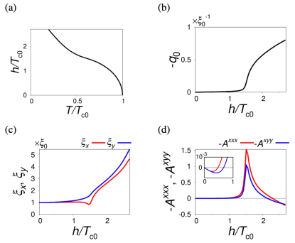
Figure 1: (a) The transition line $({T_{\rm c}}(h),h)$ of the $s$-wave Rashba-Zeeman superconductor, (b) Cooper-pair momentum $-q_{0}$, (c) GL coherence length $\xi_{x},\xi_{y}$, and (d) anharmonicity parameters $-{\mathcal{A}}^{xxx},-{\mathcal{A}}^{xyy}$ along the transition line $({T_{\rm c}}(h),h)$. $\xi_{x},\xi_{y}$ and $q_{0}^{-1}$ are in units of $\xi_{0}$, i.e. $\xi_{x}$ and $\xi_{y}$ at $h=0$. The increasing tendency in $\xi_{x}$ and $\xi_{y}$ comes from the decrease of $T_{c}(h)$. The inset of (d) shows the region $0\leq h/{T_{\rm c0}}\leq 1$.

While the coherence length $\xi_{x}$ and $\xi_{y}$ are always of the same order in magnitude [Fig. 1(c)], the anharmonicity parameters ${\mathcal{A}}^{xxx}$ and ${\mathcal{A}}^{xyy}$ are extremely enhanced in the crossover region as shown in Fig. 1(d): The rapid change in $\bm{q}_{0}$ naturally accompanies the anomalous $\bm{q}$ dependence of $\alpha_{\bm{q}}$ around there. The inset shows that ${\mathcal{A}}^{xxx}$ and ${\mathcal{A}}^{xyy}$ have tiny linear slopes under the small magnetic field $h$, as expected. The $h$-linear behavior is limited to the low-field region, and thus, the nonlinear effects are essential. The high-field behavior is discussed below.

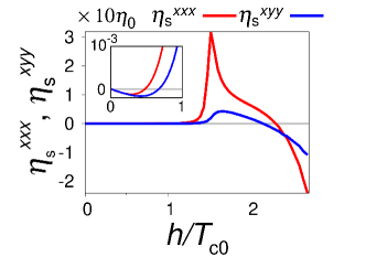
Figure 2: Strength of the rectification $\eta^{xxx}_{\rm{s}}$ and NHE $\eta^{xyy}_{\rm{s}}$ in the $s$-wave Rashba-Zeeman superconductor along the transition line $({T_{\rm c}}(h),h)$. The inset shows the region $0\leq h/{T_{\rm c0}}\leq 1.$

The huge increase of the anharmonicity parameters naturally enhances rectification and NHE as shown in Fig. 2: Both $\eta^{xxx}_{\rm{s}}$ and $\eta^{xyy}_{\rm{s}}$ are increased by several orders of magnitude along the transition line. The enhancement of $\eta^{xxx}_{\rm{s}}$ compared to $\eta^{xyy}_{\rm{s}}$ originates from the increased anisotropy $\xi_{y}/\xi_{x}$ in the crossover region [see Fig. 1(c) and Eq. (14)]. Similar results are obtained for various parameters and for the $d$-wave states [70]. The obtained values of $\eta_{\rm{s}}^{ijk}$ are comparable in units of $\eta_{0}\equiv L_{z}\xi_{0}/{T_{\rm c0}}$, implying large NCT in superconductors with small ${T_{\rm c0}}$ and large $\xi_{0}$. For the case of heavy-fermion superlattices [66], we obtain $\eta_{\rm{s}}^{xxx}\sim 10\eta_{\rm{s}}^{xyy}\sim 10^{-2}\ \mathrm{\mu m^{2}/\mu A}$ with assuming $\xi_{0}\sim 5\ \mathrm{nm}$, ${T_{\rm c0}}\sim 2\ \mathrm{K}$, and $L_{z}\sim 10\ \mathrm{nm}$. This means that $10\%$ rectification is obtained under the current density $\sim 10\ \mathrm{\mu A/\mu m^{2}}$ at the mean-field transition temperature. Typical values of the nonlinear resistivity in the fluctuation regime are estimated to be $\rho^{xxx}_{2*}\sim 10\rho^{xyy}_{2*}\sim 10^{-4}\ \Omega\mathrm{\mu m^{3}/\mu A}$ with assuming $\sigma_{1{\rm{n}}}^{-1}\sim 5\times 10^{-7}\ \Omega\mathrm{m}$. These values are well within the experimental scope, and thus rectification and NHE serve as promising probes to capture helical-superconductivity crossover.

Interestingly, the anharmonicity parameters take slightly smaller but still sizable values under higher magnetic fields [$h/{T_{\rm c0}}\gtrsim 2.5$ in Fig. 1(d)]. Large rectification and NHE are obtained there in combination with small ${T_{\rm c}}(h)$ [Fig. 2], while the sign reversal seen in Fig. 2 may be absent or shifted to higher fields, depending on model parameters [70]. It is known that the high-field helical superconductivity resembles in nature the Flude-Ferrell-Larkin-Ovchinnikov (FFLO) state of centrosymmetric superconductors [37]. Thus, our results imply that FFLO state, and possibly the pair-density-wave states, might show giant NCT once the symmetry-protected degeneracy of Cooper-pair momenta is externally lifted. From symmetry viewpoints, this could be achieved by the out-of-plane bias voltage and inplane magnetic field (the same symmetry as helical superconductivity). Quantitative studies are awaited for candidate materials such as cuprate thin films [52, 73, 74, 75, 76].

Orbital magnetic field. — We have pointed out that colossal rectification and NHE are promising probes of thin-film helical superconductors. A natural question is then whether the conclusion still holds in quasi-two-dimensional superconductors where the cyclotron motion of fluctuating Cooper pairs takes place. To study this problem, we have derived a Kubo-type formula of $\sigma_{2{\rm{s}}}^{ijk}$ for the time-dependent GL equation of the form $\Gamma_{0}\frac{\partial}{\partial t}\ket{\psi(t)}=\hat{\alpha}\ket{\psi(t)}+\ket{\zeta(t)}$:

$$\!\!\!\!\sigma_{2{\rm{s}}}^{ijk} =\frac{2\Gamma_{0}^{2}}{\beta V}\sum_{\mu\nu\lambda}\frac{J_{\mu\nu\lambda}^{ijk}(\alpha_{\mu}+\alpha_{\nu}+2\alpha_{\lambda})}{\alpha_{\lambda}(\alpha_{\mu}+\alpha_{\nu})(\alpha_{\mu}+\alpha_{\lambda})^{2}(\alpha_{\nu}+\alpha_{\lambda})^{2}},$$ (15)

with $\hat{\alpha}\ket{\mu}=\alpha_{\mu}\ket{\mu}$, $J_{\mu\nu\lambda}^{ijk}=\mathrm{Re}[\braket{\mu}{j_{i}}{\nu}\braket{\nu}{j_{j}}{\lambda}\braket{\lambda}{j_{k}}{\mu}]$, and $j_{i}=-\partial_{A_{i}}\hat{\alpha}$ [70]. This general formula of the phenomenological nonlinear paraconductivity is applicable to e.g., systems with orbital magnetic fields as well as multiple pairing channels.

Let us consider bulk noncentrosymmetric superconductors under the magnetic field $B$ in the $y$ direction, which can be described by $\hat{\alpha}=\alpha_{\bm{q}}|_{\bm{q}\to\nabla/i-2\bm{A}(\bm{x})}$ [69, 77, 33]. We focus on the first-order effect of ${\mathcal{A}}^{xxx}$ and ${\mathcal{A}}^{xyy}$ for the purpose of an order estimate of NCT [70],

$$\sigma_{2{\rm{s}}}^{xxx} =\frac{\tau_{0}^{2}T}{2\pi|{\mathcal{B}}|\sqrt{\bar{\epsilon}}}\,{\mathcal{A}}^{xxx},\quad\sigma_{2{\rm{s}}}^{xyy}=\frac{3\tau_{0}^{2}T}{4\pi\bar{\epsilon}^{3/2}}\,{\mathcal{A}}^{xyy},$$ (16)

where ${\mathcal{B}}\equiv B\xi_{x}\xi_{z}$ is the magnetic flux threading the area spanned by the coherence length. The most singular terms regarding the reduced temperature under the magnetic field $\bar{\epsilon}\equiv\epsilon+2|{\mathcal{B}}|=(T-{T_{\rm c}}(B))/T$ are kept here, while $\sigma_{2{\rm{s}}}^{yxy}=\sigma_{2{\rm{s}}}^{yyx}=\sigma_{2{\rm{s}}}^{xyy}/2$ is obtained to the leading order of $\bar{\epsilon}$. Equations (16) indicate that the orbital magnetic field suppresses the singularity of rectification perpendicular to the field while leaving that of NHE intact [compare Eq. (16) with Eq. (8b)]. See Supplemental Material for more details of NCT under the orbital magnetic field.

The obtained expressions of NCT are proportional to ${\mathcal{A}}^{ijk}$, implying that the rapid increase of NCT occurs in bulk samples as well, triggered by the helical-superconductivity crossover. To estimate the nonreciprocity in the fluctuation regime, we discuss $\eta_{*}^{xxx}\equiv\rho_{2*}^{xxx}/\rho_{1*}^{xx}$ since $\eta_{{\rm{s}}}^{xxx}$ vanishes. At the reduced temperature defined by $\sigma_{1{\rm{s}}}^{xx}({\bar{\epsilon}}_{*})=\sigma_{1{\rm{n}}}^{xx}/3$, we obtain the nonreciprocity $\eta_{*}^{xxx}\sim 10^{-5}{\rm\mu m^{2}/\mu A}$ for layered helical superconductors in the crossover region, by using the coherence lengths $\xi_{x}\sim\xi_{y}/2\sim 5\ {\rm nm}$, $\xi_{z}\sim 2\ {\rm nm}$, relaxation time $\tau_{0}\sim\pi/8T$, and $B\sim 2{T_{\rm c0}}\sim{0.4}\ {\rm m}e{\rm V}$, as well as ${\mathcal{A}}^{xxx}$ estimated from Fig. 1(d). NHE can be estimated similarly [70]. The obtained rectification and NHE $\rho^{xxx}_{2*}\sim\rho^{xyy}_{2*}\sim 10^{-5}\ \Omega\mathrm{\mu m^{3}/\mu A}$ are smaller than those of two-dimensional systems but are still observable when the fluctuation regime is visible for the experimental resolution of temperature [78].

In combination with the results for atomically-thin superconductors, we have demonstrated that rectification and NHE in the fluctuation regime are promising probes of helical superconductivity regardless of sample dimensions. The results strongly suggest that the enhanced NCT under moderate and high magnetic fields is observable in realistic thin-film samples with a non-negligible thickness, which would lie between the two-dimensional and three-dimensional limits studied in this work. In particular, NHE would serve as a better probe because the linear Hall resistance is absent owing to the $y$-mirror symmetry. Furthermore, the vortex motion below the mean-field transition temperature might be suppressed by the force-free configuration, to allow easier access to the intrinsic contribution. Material-based study for the candidate helical superconductors [65, 66, 67, 68] is left as an intriguing future issue, as well as the fully-microscopic treatment of NCT including the quantum-mechanical corrections beyond the GL approach.

I Derivation of the fluctuation conductivity

The derivation of the fluctuation conductivity without the orbital magnetic field can be performed following Ref. [6] with a straightforward generalization. For clarity, we show the details below.

I.1 Setup

We start from the time-dependent GL (TDGL) equation

$$\Gamma_{0}\frac{\partial\psi(\bm{x},t)}{\partial t}=-\frac{\delta F[\psi,\psi^{*}]}{\delta\psi^{*}(\bm{x})}+\zeta(\bm{x},t).$$ (17)

Here, the GL functional is assumed to be the bilinear of the order parameter,

$$F[\psi] =\int d^{d}x\int d^{d}x^{\prime}\psi^{*}(\bm{x})\alpha(\bm{x}-\bm{x}^{\prime})\psi(\bm{x}^{\prime}),$$ (18)

describing the Gaussian fluctuation of Cooper pairs. The phenomenological parameter $\Gamma_{0}$ takes into account the relaxation process of Cooper pairs. In the absence of the electric field, TDGL has the equilibrium solution $\delta F/\delta\psi^{*}=0$ as its steady state, if $\zeta(\bm{x},t)$ is neglected. The random force $\zeta(\bm{x},t)$ kicks up the fluctuation of the order parameter $\psi(\bm{x},t)$, which vanishes after a finite lifetime $\propto\Gamma_{0}/(T-{T_{\rm c}})$.

It is convenient to switch to the momentum space for our purpose. We adopt the following convention of the Fourier transform:

$$\psi_{\bm{q}}(t) =\frac{1}{V}\int d^{d}x\,e^{-i\bm{q}\cdot\bm{x}}\psi(\bm{x},t),$$ (19a)

$$\zeta_{\bm{q}}(t) =\frac{1}{V}\int d^{d}x\,e^{-i\bm{q}\cdot\bm{x}}\zeta(\bm{x},t).$$ (19b)

Here, the momentum is $\bm{q}\in\prod_{i=1}^{d}(2\pi\mathbb{Z}/L_{i})$ with assuming the periodic boundary conditions, with $L_{i}$ the diameter in the $i$ direction. The system volume in the $d$ dimensions is defined by $V=\prod_{i=1}^{d}L_{i}$. With this notation, $\psi_{\bm{q}=0}$ coincides with the spatial average of the order parameter. The GL coefficient in the Fourier space is defined by

$$\alpha_{\bm{q}} =\int d^{d}x\,e^{-i\bm{q}\cdot\bm{x}}\alpha(\bm{x}),$$ (20)

leading to the GL functional

$$F[\psi] =V\sum_{\bm{q}}\alpha_{\bm{q}}|\psi_{\bm{q}}|^{2}.$$ (21)

This gives the equilibrium average of the order parameter

$$\braket{}{\psi_{\bm{q}}}{{}^{2}} =\frac{\int D[\psi,\psi^{*}]e^{-\beta F[\psi]}|\psi_{\bm{q}}|^{2}}{\int D[\psi,\psi^{*}]e^{-\beta F[\psi]}}$$

$$=\frac{1}{\beta V\alpha_{\bm{q}}},$$ (22)

with the inverse temperature $\beta\equiv 1/T$.

With the conventions introduced above, the TDGL equation in the momentum space is given by

$$\Gamma_{0}\frac{\partial\psi_{\bm{q}}(t)}{\partial t} =-\alpha_{\bm{q}}\psi_{\bm{q}}(t)+\zeta_{\bm{q}}(t).$$ (23)

It should be noted that $\Gamma_{0}$ can generally depend on $\bm{q}$ and external parameters such as $\bm{h}$ from the microscopic viewpoint. While the latter dependence is canceled out in the nonreciprocity $\eta_{\rm{s}}^{ijk}$ in two dimensions, the $\bm{q}$ dependence of $\Gamma_{0}$ is neglected for simplicity in this paper, which is left as the future issue [fully microscopic treatment would be more suitable to account for such effects]. For the time being, we assume $\Gamma_{0}\in\mathbb{C}$ with $\mathrm{Re}[\Gamma_{0}]>0$ for generality, while the imaginary part is expected to be small in the absence of the strong particle-hole asymmetry of the density of states [69].

The general solution of the TDGL equation is given by

$$\psi_{\bm{q}}(t) =e^{-\frac{1}{\Gamma_{0}}\int_{t_{0}}^{t}dt^{\prime}\,\alpha_{\bm{q}}(t^{\prime})}\psi_{\bm{q}}(t_{0})$$

$$+\frac{1}{\Gamma_{0}}\int_{t_{0}}^{t}dt^{\prime}\,e^{-\frac{1}{\Gamma_{0}}\int_{t^{\prime}}^{t}dt^{\prime\prime}\,\alpha_{\bm{q}}(t^{\prime\prime})}\zeta_{\bm{q}}(t^{\prime}),$$ (24)

where $\alpha_{\bm{q}}(t)\equiv\alpha_{\bm{q}-2\bm{A}(t)}$ when the electric field is applied to the system. After a sufficiently large period $(t-t_{0})\alpha_{\bm{q}}\gg\mathrm{Re}[\Gamma_{0}]$, the order parameter becomes independent of the initial condition. We are interested in such a situation, and thus take the limit $t_{0}\to\infty$ and drop the first term. Thus, we obtain

$$\braket{}{\psi_{\bm{q}}(t)}{{}^{2}} =\int_{-\infty}^{0}dt_{1}\int_{-\infty}^{0}dt_{2}\,e^{-\left[\int_{t_{1}}^{0}\frac{1}{\Gamma_{0}^{*}}+\int_{t_{2}}^{0}\frac{1}{\Gamma_{0}}\right]dt^{\prime}\,\alpha_{\bm{q}}(t+t^{\prime})}$$

$$\qquad\qquad\cdot\frac{1}{|\Gamma_{0}|^{2}}\braket{\xi^{*}_{\bm{q}}(t+t_{1})\zeta_{\bm{q}}(t+t_{2})}.$$ (25)

The average over the white noise is defined to reproduce Eq. (22) by the TDGL equation in equilibrium, i.e. $\bm{E}=0$:

$$\braket{\xi^{*}_{\bm{q}}(t)\xi_{\bm{q}^{\prime}}(t^{\prime})} =\frac{2\mathrm{Re}[\Gamma_{0}]}{\beta V}\delta(t-t^{\prime})\delta_{\bm{q},\bm{q}^{\prime}}.$$ (26)

With this, we obtain the excess electric current density [71]

$$\bm{j}_{\rm{s}}(t) \equiv-\sum_{\bm{q}}\partial_{\bm{A}}\alpha_{\bm{q}-2\bm{A}(t)}\braket{}{\psi_{\bm{q}}(t)}{{}^{2}}$$ (27)

$$=\frac{4\mathrm{Re}[\Gamma_{0}]}{|\Gamma_{0}|^{2}\beta}\int\frac{d^{d}q}{(2\pi)^{d}}\partial_{\bm{q}}\alpha_{\bm{q}}\int^{0}_{-\infty}dt_{1}\,e^{-\frac{2\mathrm{Re}[\Gamma_{0}]}{|\Gamma_{0}|^{2}}\int^{0}_{t_{1}}dt^{\prime}\,\alpha_{\bm{q}-2\bm{A}(t^{\prime})}}.$$

To be precise, $\bm{j}_{\rm{s}}(t)$ in the left hand side should be understood as the current $\bm{j}_{\rm{s}}(t)L_{y}L_{z}$ and the sheet current density $\bm{j}_{\rm{s}}(t)L_{z}$ for $d=1$ and $2$, respectively, rather than the current density. This point is taken into account at the end of the calculation. Note also that by redefining $|\Gamma_{0}|^{2}/\mathrm{Re}[\Gamma_{0}]\to\Gamma_{0}$ the expression of $\bm{j}_{\rm{s}}(t)$ coincides with that for the situation with $\mathrm{Im}[\Gamma_{0}]=0$. Thus, we consider the case $\Gamma_{0}>0$ in the following and in the main text without loss of generality.

I.2 Expansion by the electric field

Let us expand $\bm{j}_{\rm{s}}(t)$ in terms of $\bm{E}$ to obtain linear and nonlinear conductivity. We start from

$$\bm{j}_{\rm{s}}(t) =\frac{4}{\beta}\int\frac{d^{d}q}{(2\pi)^{d}}\partial_{\bm{q}}\alpha_{\bm{q}}\int^{0}_{-\infty}dt_{1}\,e^{2\int_{0}^{t_{1}}dt^{\prime}\,\alpha_{\bm{q}-2\bm{A}(t^{\prime})}},$$ (28)

where the domain of the $\bm{q}$ integral is the first Brillouin zone. Here, we made the replacement $\alpha/\Gamma_{0}\to\alpha$ for simplicity. We will recover the effect of $\Gamma_{0}$ at the end of the calculation by $\alpha\to\alpha/\Gamma_{0}$. The exponent of the exponential is given by

$$\int_{0}^{t_{1}}dt^{\prime}\,\alpha_{\bm{q}-2\bm{A}(t^{\prime})} =\alpha_{\bm{q}}t_{1}+t_{1}^{2}E_{i}\partial_{q_{i}}\alpha_{\bm{q}}$$

$$\quad+\frac{2}{3}t_{1}^{3}E_{i}E_{j}\partial_{q_{i}}\partial_{q_{j}}\alpha_{\bm{q}}+O(E^{3}),$$ (29)

and thus we can write

$$\!\!\!\!\int^{0}_{-\infty}dt_{1}\,e^{2\int_{0}^{t_{1}}dt^{\prime}\,\alpha_{\bm{q}-2\bm{A}(t^{\prime})}} \equiv A_{0}+A_{1}+A_{2}+O(E^{3}),$$ (30)

with

$$A_{0} \equiv\int_{0}^{\infty}dt_{1}\,e^{-2t_{1}\alpha_{\bm{q}}}=1/2\alpha_{\bm{q}},$$ (31a)

$$A_{1} \equiv\int_{0}^{\infty}dt_{1}\,2t_{1}^{2}E_{j}\partial_{q_{j}}\alpha_{\bm{q}}\,e^{-2t_{1}\alpha_{\bm{q}}}$$

$$=\frac{\partial_{q_{j}}\alpha_{\bm{q}}}{2\alpha_{\bm{q}}^{3}}E_{j},$$ (31b)

$$A_{2} \equiv\int_{0}^{\infty}dt_{1}\,\Bigl{[}\frac{1}{2}(2t_{1}^{2}E_{j}\partial_{q_{j}}\alpha_{\bm{q}})^{2}$$

$$\qquad\qquad-\frac{4}{3}t_{1}^{3}E_{j}E_{k}\partial_{q_{j}}\partial_{q_{k}}\alpha_{\bm{q}}\Bigr{]}e^{-2t_{1}\alpha_{\bm{q}}}$$

$$=E_{j}E_{k}\left[\frac{3}{2}\frac{\partial_{q_{j}}\alpha_{\bm{q}}\partial_{q_{k}}\alpha_{\bm{q}}}{\alpha_{\bm{q}}^{5}}-\frac{\partial_{q_{j}}\partial_{q_{k}}\alpha_{\bm{q}}}{2\alpha_{\bm{q}}^{4}}\right].$$ (31c)

The contribution from $A_{0}$ is a total derivative of the momentum and therefore vanishes according to the periodicity of the Brillouin zone. This means that the electric current is absent in equilibrium. In the following, we evaluate the linear and nonlinear fluctuation conductivity tensors determined by $A_{1}$ and $A_{2}$.

I.3 Linear fluctuation conductivity

We first discuss the linear fluctuation conductivity described by $A_{1}$,

$$\sigma_{1{\rm{s}}}^{ij} =\frac{2}{\beta}\int\frac{d^{d}q}{(2\pi)^{d}}\frac{\partial_{q_{i}}\alpha_{\bm{q}}\partial_{q_{j}}\alpha_{\bm{q}}}{\alpha_{\bm{q}}^{3}}.$$ (32)

Since $\alpha_{\bm{q}_{0}}\equiv\min_{\bm{q}}\alpha_{\bm{q}}\to+0$ as $T\to{T_{\rm c}}+0$, the contribution around $\bm{q}=\bm{q}_{0}$ diverges and dominates the momentum integral. Therefore, we can neglect the information on the high-energy modes: We can only consider the domain of the integral $|\bm{q}-\bm{q}_{0}|<O({q_{\rm c}})$ with a small cut-off ${q_{\rm c}}$ to obtain $\sigma_{1}^{ij}$ to the leading order of $\alpha_{\bm{q}_{0}}$. Near $\bm{q}=\bm{q}_{0}$, we can write $\alpha_{\bm{q}}$ as

$$\alpha_{\bm{q}} =\alpha_{\bm{q}_{0}}+\alpha_{2}^{ij}\delta q_{i}\delta q_{j}+\alpha_{3}^{ijk}\delta q_{i}\delta q_{j}\delta q_{k}+O(\delta q^{4}),$$ (33)

with $\delta\bm{q}\equiv\bm{q}-\bm{q}_{0}$. Note that ${q_{\rm c}}$ should be sufficiently small to allow the Taylor expansion of $\alpha_{\bm{q}}$ while sufficiently large to capture the contribution around $\bm{q}_{0}$. It turns out that we can choose e.g., ${q_{\rm c}}=O(\alpha_{\bm{q}_{0}}^{1/24})$ for our purpose. With this choice, the contribution from the outside of the domain is at most of the order $\alpha^{-3}_{\bm{q}}\sim{q_{\rm c}}^{-6}\sim\alpha_{\bm{q}_{0}}^{-1/4}$, which is smaller than the leading term of $\sigma_{1}^{ij}=O(\alpha_{\bm{q}_{0}}^{-(2-d/2)})$ as obtained in the following.

For practical calculations, we rewrite the expansion of $\alpha_{\bm{q}}$ as follows:

$$\alpha_{\bm{q}} =\epsilon+\sum_{i}\xi_{i}^{2}\delta q_{i}^{2}+\bar{\xi}\,{}^{3}\sum_{ijk}\mathcal{A}^{ijk}\delta q_{i}\delta q_{j}\delta q_{k}$$ (34)

$$=\epsilon+\sum_{i}(\xi_{i}\delta q_{i})^{2}+\sum_{ijk}a_{3}^{ijk}(\xi_{i}\delta q_{i})(\xi_{j}\delta q_{j})(\xi_{k}\delta q_{k}),$$

with the reduced temperature $\epsilon$ and the coherence length $\xi_{i}$. Note that we are temporarily setting $N_{0}=T\partial_{T}\alpha_{\bm{q}_{0}}\to 1$. This can be recovered by the replacement $\Gamma_{0}\to\tau_{0}$ at the end of the calculation. The coordinate axes are chosen to diagonalize the symmetric tensor $\alpha_{2}^{ij}=\xi_{i}^{2}\delta_{ij}$ with $\xi_{i}>0$. For the later convenience, we introduce $a_{3}^{ijk}=\bar{\xi}^{3}{\mathcal{A}}^{ijk}/(\xi_{i}\xi_{j}\xi_{k})$ instead of the anharmonicity parameter ${\mathcal{A}}^{ijk}$. For the linear paraconductivity, however, the $a_{3}^{ijk}$ term is not necessary to obtain the leading-order contribution, since $\sigma_{1{\rm{s}}}^{ij}$ becomes finite without $a_{3}^{ijk}$ and the contribution from $a_{3}^{ijk}$ is smaller than the $\delta q^{2}$ terms by at least $O({q_{\rm c}})\ll 1$. Higher-order Taylor coefficients of $\alpha_{\bm{q}}$, if considered, are also irrelevant for the same reason. By using $p_{i}\equiv\xi_{i}\delta q_{i}$ and then $p_{i}\to\sqrt{\epsilon}\,p_{i}$, we obtain

$$\sigma_{1{\rm{s}}}^{ij} =\frac{8T}{\epsilon^{2-d/2}}\frac{\xi_{i}\xi_{j}}{\bar{\xi}^{d}}\int\frac{d^{d}p}{(2\pi)^{d}}\frac{p_{i}p_{j}}{(1+p^{2})^{3}}$$

$$=\begin{cases}\frac{1}{L_{y}L_{z}}\frac{\tau_{0}T\xi_{x}}{2\epsilon^{3/2}}&(d=1)\\ \frac{1}{L_{z}}\frac{\tau_{0}T}{2\pi\epsilon}\frac{\xi_{i}^{2}}{\bar{\xi}^{2}}\delta_{ij}&(d=2)\\ \frac{\tau_{0}T}{4\pi\sqrt{\epsilon}}\frac{\xi_{i}^{2}}{\bar{\xi}{}^{3}}\delta_{ij}&(d=3)\end{cases},$$ (35)

reproducing the results in Ref. [69] by $\tau_{0}\to\pi/8T$. Here, the domain of $\bm{p}$ integral is set to $\mathbb{R}^{d}$ since $\xi_{i}{q_{\rm c}}/\sqrt{\epsilon}\gg 1$: The contribution from the interval $\xi{q_{\rm c}}/\sqrt{\epsilon}<|p|<\infty$ is negligible compared with that from $\mathbb{R}^{d}$. We recovered the effect of $\Gamma_{0}$ in the last line by multiplying $\tau_{0}$, considering the expression of Eq. (32). The factors $1/L_{y}L_{z}$ and $1/L_{z}$ are taken into account in the final expression for $d=1,2$ as noted previously. For general choice of the coordinate axes, we can use the tensor expression

$$\sigma_{1{\rm{s}}}^{ij} =\begin{cases}\frac{1}{L_{z}}\frac{\Gamma_{0}T}{2\pi\alpha_{\bm{q}_{0}}}\frac{\alpha_{2}^{ij}}{\sqrt{\det[\alpha_{2}]}}&(d=2)\\ \frac{\Gamma_{0}T}{4\pi\sqrt{\alpha_{\bm{q}_{0}}}}\frac{\alpha_{2}^{ij}}{\sqrt{\det[\alpha_{2}]}}&(d=3)\end{cases}.$$ (36)

I.4 Nonlinear fluctuation conductivity

Next, we evaluate the second-order fluctuation conductivity determined by $A_{2}$,

$$\beta\sigma_{2{\rm{s}}}^{ijk}E_{j}E_{k} =\int\frac{d^{d}q}{(2\pi)^{d}}\Bigl{[}6\,\frac{\partial_{q_{i}}\alpha_{\bm{q}}\partial_{q_{j}}\alpha_{\bm{q}}\partial_{q_{k}}\alpha_{\bm{q}}}{\alpha_{\bm{q}}^{5}}$$

$$\qquad\qquad\qquad-2\,\frac{\partial_{q_{i}}\alpha_{\bm{q}}\partial_{q_{j}}\partial_{q_{k}}\alpha_{\bm{q}}}{\alpha_{\bm{q}}^{4}}\Bigr{]}E_{j}E_{k}$$

$$\equiv 6B_{1}-2B_{2}.$$ (37)

Here, $d=1,2,3$ is the system dimensions. Note that the second term is proportional to the first term. Actually,

$$B_{1} =\int\frac{d^{d}q}{(2\pi)^{d}}-\frac{1}{4}\partial_{q_{j}}[\alpha_{\bm{q}}^{-4}]\partial_{q_{i}}\alpha_{\bm{q}}\partial_{q_{k}}\alpha_{\bm{q}}E_{j}E_{k}$$

$$=\frac{1}{4}\int\frac{d^{d}q}{(2\pi)^{d}}\alpha_{\bm{q}}^{-4}[\partial_{q_{i}}\partial_{q_{j}}\alpha_{\bm{q}}\partial_{q_{k}}\alpha_{\bm{q}}$$

$$\qquad+\partial_{q_{i}}\alpha_{\bm{q}}\partial_{q_{j}}\partial_{q_{k}}\alpha_{\bm{q}}]E_{j}E_{k}$$

$$\equiv\frac{1}{4}B_{2}^{\prime}+\frac{1}{4}B_{2}.$$ (38)

Here, we defined

$$B_{2}^{\prime} \equiv\int\frac{d^{d}q}{(2\pi)^{d}}\alpha_{\bm{q}}^{-4}\partial_{q_{i}}\partial_{q_{j}}\alpha_{\bm{q}}\partial_{q_{k}}\alpha_{\bm{q}}E_{j}E_{k}$$

$$=4\int\frac{d^{d}q}{(2\pi)^{d}}\alpha_{\bm{q}}^{-5}\partial_{q_{i}}\alpha_{\bm{q}}\partial_{q_{j}}\alpha_{\bm{q}}\partial_{q_{k}}\alpha_{\bm{q}}E_{j}E_{k}$$

$$\quad-\int\frac{d^{d}q}{(2\pi)^{d}}\alpha_{\bm{q}}^{-4}\partial_{q_{j}}\alpha_{\bm{q}}\partial_{q_{i}}\partial_{q_{k}}\alpha_{\bm{q}}E_{j}E_{k}$$

$$=4B_{1}-B_{2}^{\prime}.$$ (39)

Thus, we obtain $B_{2}=2B_{1}$ and

$$\beta\sigma_{2{\rm{s}}}^{ijk} =B_{2}=\int\frac{d^{d}q}{(2\pi)^{d}}\frac{\partial_{q_{i}}\alpha_{\bm{q}}\partial_{q_{j}}\partial_{q_{k}}\alpha_{\bm{q}}}{\alpha_{\bm{q}}^{4}}.$$ (40)

To evaluate the momentum integral, we again focus on the region $|\delta\bm{q}|<O({q_{\rm c}})=O(\alpha_{\bm{q}_{0}}^{1/24})$, since the contribution from the outside is at most $O(\alpha_{\bm{q}_{0}}^{-8/24})\ll\sigma_{2}^{ijk}=O(\alpha_{\bm{q}_{0}}^{-(3-d/2)})$ as clarified below.

Note that $B_{2}$ vanishes in the absence of $a_{3}^{ijk}$, since the integrand becomes odd in $\delta\bm{q}$. Thus, we are interested in the correction by $a_{3}^{ijk}$. It is sufficient to keep only the first-order terms in $a_{3}^{ijk}$ to obtain the leading-order singularity of $\sigma_{2}^{ijk}$, since the correction is smaller at least by $O({q_{\rm c}})$. By using the variable $\xi_{i}\delta q_{i}=p_{i}$, we obtain

$$\partial_{q_{i}}\alpha_{\bm{q}}\partial_{q_{j}}\partial_{q_{k}}\alpha_{\bm{q}}$$

$$\simeq\xi_{i}\xi_{j}\xi_{k}[4p_{i}\delta_{jk}+12a_{3}^{jkc}p_{i}p_{c}+6\delta_{jk}a_{3}^{ibc}p_{b}p_{c}],$$

$$\alpha_{\bm{q}}^{-4} \simeq\frac{1}{(\epsilon+p^{2})^{4}}\left(1-4\frac{a_{3}^{abc}p_{a}p_{b}p_{c}}{\epsilon+p^{2}}\right).$$ (41)

After plugging these expressions into $B_{2}$ and $p_{i}\to\sqrt{\epsilon}\,p_{i}$, we can now set the domain of integral to $\mathbb{R}^{d}$. The term $B_{2}$ is then given by

$$B_{2} =\frac{\xi_{i}\xi_{j}\xi_{k}}{\epsilon^{3-d/2}(2\pi)^{d}\bar{\xi}\,{}^{d}}\int d\Omega\,\Bigl{(}$$

$$\quad\left[12\int_{0}^{\infty}dp\,\frac{p^{2+d-1}}{(1+p^{2})^{4}}\right]a_{3}^{jkc}n_{i}n_{c}$$

$$\quad+\left[6\int_{0}^{\infty}dp\,\frac{p^{2+d-1}}{(1+p^{2})^{4}}\right]\delta_{jk}a_{3}^{ibc}n_{b}n_{c}$$ (42)

$$\qquad-\left[16\int_{0}^{\infty}dp\,\frac{p^{4+d-1}}{(1+p^{2})^{5}}\right]n_{i}\delta_{jk}a_{3}^{abc}n_{a}n_{b}n_{c}\Bigr{)},$$

where $\bm{n}=(\sin\theta\cos\phi,\sin\theta\sin\phi,\cos\theta)$ and $d\Omega=\sin\theta d\theta d\phi$ for $d=3$; $\bm{n}=(\cos\theta,\sin\theta)$ and $d\Omega=d\theta$ for $d=2$; and $\int d\Omega\to 2$ and $n_{i}\to 1$ for $d=1$. The momentum integrals are evaluated by

$$\int_{0}^{\infty}dp\,\frac{p^{2+d-1}}{(1+p^{2})^{4}} =\begin{cases}\frac{\pi}{32}&(d=1)\\ \frac{1}{12}&(d=2)\\ \frac{\pi}{32}&(d=3),\end{cases}$$ (43a)

$$\int_{0}^{\infty}dp\,\frac{p^{4+d-1}}{(1+p^{2})^{5}} =\begin{cases}\frac{3\pi}{256}&(d=1)\\ \frac{1}{24}&(d=2)\\ \frac{5\pi}{256}&(d=3).\end{cases}$$ (43b)

Thus, we obtain

$$B_{2}^{d=1} =\frac{3\xi_{x}^{2}}{8\epsilon^{5/2}}a_{3}^{xxx},$$ (44)

for $d=1$,

$$B_{2}^{d=2} =\frac{\xi_{i}\xi_{j}\xi_{k}}{\epsilon^{2}(2\pi)^{2}\bar{\xi}^{2}}\int d\theta\,a_{3}^{jkc}n_{i}n_{c}+\frac{1}{2}\delta_{jk}a_{3}^{ibc}n_{b}n_{c}$$

$$\qquad-\frac{2}{3}n_{i}\delta_{jk}a_{3}^{abc}n_{a}n_{b}n_{c}$$

$$=\frac{\xi_{i}\xi_{j}\xi_{k}}{\epsilon^{2}(2\pi)^{2}\bar{\xi}^{2}}\,\pi a_{3}^{ijk},$$ (45)

for $d=2$, and

$$B_{2}^{d=3} =\frac{\xi_{i}\xi_{j}\xi_{k}}{\epsilon^{3/2}(2\pi)^{3}\bar{\xi}^{3}}\frac{\pi}{32}\int d\Omega\,12a_{3}^{jkc}n_{i}n_{c}$$

$$\quad+6\delta_{jk}a_{3}^{ibc}n_{b}n_{c}-16\cdot\frac{5}{8}n_{i}\delta_{jk}a_{3}^{abc}n_{a}n_{b}n_{c}$$

$$=\frac{\xi_{i}\xi_{j}\xi_{k}}{32\pi\epsilon^{3/2}\bar{\xi}^{3}}\,2a_{3}^{ijk},$$ (46)

for $d=3$. The angular integrals were carried out by employing Mathematica, while the case of $d=2$ is also confirmed by hand. Thus, we obtain

$$\sigma_{2{\rm{s}}}^{xxx} =\frac{1}{L_{y}L_{z}}\frac{3\tau_{0}^{2}T\xi_{x}^{2}}{8\epsilon^{5/2}}{\mathcal{A}}^{xxx}\quad(d=1),$$ (47a)

$$\sigma_{2{\rm{s}}}^{ijk} =\frac{1}{L_{z}}\frac{\tau_{0}^{2}T\bar{\xi}}{4\pi\epsilon^{2}}{\mathcal{A}}^{ijk}\quad(d=2),$$ (47b)

$$\sigma_{2{\rm{s}}}^{ijk} =\frac{\tau_{0}^{2}T}{16\pi\epsilon^{3/2}}{\mathcal{A}}^{ijk}\quad(d=3),$$ (47c)

with reproducing the effect of $\Gamma_{0}$ by multiplying $\tau_{0}^{2}$ [see Eq. (40)] as well as $1/L_{y}L_{z}$ and $1/L_{z}$ for $d=1$ and $2$, respectively. These expressions are valid for an arbitrary choice of the coordinate axes since $\bar{\xi}$ and ${\mathcal{A}}^{ijk}$ are the scalar and tensor, respectively, while we can also write

$$\sigma_{2{\rm{s}}}^{ijk} =\frac{1}{L_{z}}\frac{\Gamma_{0}^{2}T\alpha_{3}^{ijk}}{4\pi\alpha_{\bm{q}_{0}}^{2}\sqrt{\det[\alpha_{2}]}}\quad(d=2),$$ (48a)

$$\sigma_{2{\rm{s}}}^{ijk} =\frac{\Gamma_{0}^{2}T\alpha_{3}^{ijk}}{16\pi\alpha_{\bm{q}_{0}}^{3/2}\sqrt{\det[\alpha_{2}]}}\quad(d=3),$$ (48b)

by using $\alpha_{2}^{ij}$ and $\alpha_{3}^{ijk}$. In particular, the intrinsic nonreciprocity in two-dimensional systems is given by

$$\eta_{\rm{s}}^{ijk} =-L_{z}\frac{\pi\bar{\xi}}{T}\frac{\bar{\xi}{}^{4}}{\xi_{j}^{2}\xi_{k}^{2}}{\mathcal{A}}^{ijk}\quad(d=2).$$ (49)

The expression for the arbitrary choice of the coordinate axes is given by

$$\eta_{2{\rm{s}}}^{ijk} =-L_{z}\frac{\pi\sqrt{\det[\alpha_{2}]}}{T}\alpha_{3}^{ibc}[\alpha_{2}^{-1}]_{bj}[\alpha_{2}^{-1}]_{ck}\quad(d=2).$$ (50)

II Angle dependence of NCT under small magnetic fields

As noted in the main text, MCA by the fluctuation contribution is determined by the effective cubic spin-orbit coupling $\bm{g}_{3}(\bm{k})$. For example in Rashba and Ising systems, this is given by $\sim(k_{x}^{2}+k_{y}^{2})(-k_{y},k_{x},0)$ and $\sim(0,0,k_{y}^{3}-3k_{y}k_{x}^{2})$. It follows that $\bm{g}_{3}(\hat{E})=(\hat{E}_{x}^{2}+\hat{E}_{y}^{2})\hat{z}\times\hat{E}=\hat{z}\times\hat{E}$ and $\bm{g}_{3}(\hat{E})=\hat{z}(\sin^{3}\theta-3\sin\theta\cos^{2}\theta)=-\sin 3\theta\hat{z}$ for $\hat{E}=(\cos\theta,\sin\theta,0)$, respectively. $\bm{g}_{3}(\hat{E})$ for a given antisymmetric spin-orbit coupling can be obtained in the same way.

The $\bm{h}$-linear NHE is given as follows.

$$\frac{4\pi\epsilon^{2}}{\tau_{0}^{2}T\bar{\xi}}[\hat{z}\times\hat{E}]\cdot\frac{L_{z}\delta^{2}\bm{j}_{\rm{s}}}{E^{2}}$$

$$=[\hat{z}\times\hat{E}]_{i}\hat{E}_{j}\hat{E}_{k}{\mathcal{A}}^{ijk}$$

$$=\frac{1}{3}[\hat{z}\times\hat{E}]\cdot\lim_{\bm{q}\to\hat{E}}\partial_{\bm{q}}[{\mathcal{A}}^{abc}q_{a}q_{b}q_{c}]$$

$$=\frac{1}{3}[\hat{z}\times\hat{E}]_{i}\lim_{\bm{q}\to\hat{E}}\partial_{q_{i}}\bm{g}_{3}(\bm{q})\cdot\bm{h}$$

$$=\frac{\bm{h}}{3}\cdot\lim_{\delta\to 0}\frac{\bm{g}_{3}(\hat{E}+\delta[\hat{z}\times\hat{E}])-\bm{g}_{3}(\hat{E})}{\delta}.$$ (51)

By introducing the unit vector

$$\hat{E}_{\delta\theta} \equiv\frac{(\hat{E}+\delta\theta[\hat{z}\times\hat{E}])}{\sqrt{1+\delta\theta^{2}}}=\hat{E}(\theta+\delta\theta)+o(\delta\theta),$$ (52)

we obtain

$$\frac{4\pi\epsilon^{2}}{\tau_{0}^{2}T\bar{\xi}}[\hat{z}\times\hat{E}]\cdot\frac{L_{z}\delta^{2}\bm{j}_{\rm{s}}}{E^{2}}$$

$$=\frac{\bm{h}}{3}\cdot\lim_{\delta\theta\to 0}\frac{(1+\delta\theta^{2})^{3/2}\bm{g}_{3}(\hat{E}_{\delta\theta})-\bm{g}_{3}(\hat{E})}{\delta\theta}$$

$$=\frac{\bm{h}}{3}\cdot\partial_{\theta}\bm{g}_{3}(\hat{E}(\theta)).$$ (53)

To obtain the second line, note that $\bm{g}_{3}(\bm{k})$ contains only $O(k^{3})$ terms. Thus, the formula in the main text is obtained.

Note that the obtained angle dependence is consistent with Ref. [32], which studies Rashba systems. To see this, let us consider the electric current in the $x$ direction for the Rashba system. In the presence of $C_{\infty}$ rotational symmetry assumed in Ref. [32], we obtain $\bm{g}_{3}(\bm{q})\propto(q_{x}^{2}+q_{y}^{2})(-q_{y},q_{x},0)$ and thus $\bm{g}_{3}(\hat{E})\propto\hat{z}\times\hat{E}$. We can write

$$\delta^{2}j_{{\rm{s}}}^{x} =\hat{x}\cdot\left(\hat{E}[\hat{E}\cdot\delta^{2}\bm{j}_{\rm{s}}]+[\hat{z}\times\hat{E}][\hat{z}\times\hat{E}\cdot\delta^{2}\bm{j}_{\rm{s}}]\right)$$

$$=C\Bigl{(}\cos\theta_{E}\cos(\theta_{E}+\pi/2-\theta_{h})$$

$$\qquad-\frac{1}{3}\cos(\theta_{E}+\pi/2)\cos(\theta_{E}-\theta_{h})\Bigr{)},$$ (54)

with a prefactor $C$. Here, the angles $\theta_{E}$ and $\theta_{h}$ for the electric and magnetic fields are measured from the $x$ axis. This is equivalent to

$$\delta^{2}j_{{\rm{s}}}^{x}=\frac{C}{3}\left[2\sin\theta_{h}+\sin(\theta_{h}-2\theta_{E})\right],$$ (55)

which agrees with Ref. [32].

The Rashba model studied in this paper is classified into the point group $C_{4v}$ in the absence of $\bm{h}$, and does not have the $C_{\infty}$ symmetry. In the presence of tetragonal anisotropy, we generally have another component in $\bm{g}_{3}(\bm{q})$ proportional to $(q_{x}^{2}-q_{y}^{2})(q_{y},q_{x},0)$, which breaks $C_{\infty}$ symmetry but belongs to the identity representation of $C_{4v}$. This term additionally contributes to $\bm{g}_{3}(\hat{E})$ by $C^{\prime}\cos 2\theta(\sin\theta,\cos\theta,0)$ with another prefactor $C^{\prime}$ independent of $C$. Accordingly, the field-angle dependence of $\delta^{2}j_{\rm{s}}^{x}$ may deviate from Eq. (55) in realistic materials. Such tetragonal anisotropy is also seen in our numerical results, because $3{\mathcal{A}}^{xyy}={\mathcal{A}}^{xyy}+{\mathcal{A}}^{yxy}+{\mathcal{A}}^{yyx}$ should coincide with ${\mathcal{A}}^{xxx}$ up to $O(h)$ if the anisotropy were absent.

III Details of the numerical calculations for NCT in Rashba-Zeeman model

Here we show the details of the numerical calculations of the GL coefficients in the Rashba-Zeeman model. The GL coefficients can be evaluated with the formula

$$\alpha_{\bm{q}}=\frac{\sum_{m}1}{4U_{\varphi}}+\frac{1}{2V}\sum_{\bm{k},m,n}F_{mn}(\bm{k},\bm{q})Q_{mn}(\bm{k},\bm{q}),$$ (56)

$$F_{mn}(\bm{k},\bm{q})=\frac{f\bigl{(}\epsilon_{m}(\bm{k}+\bm{q}/2)\bigr{)}-f\bigl{(}-\epsilon_{n}(-\bm{k}+\bm{q}/2)\bigr{)}}{\epsilon_{m}(\bm{k}+\bm{q}/2)+\epsilon_{n}(-\bm{k}+\bm{q}/2)},$$

$${Q_{mn}(\bm{k},\bm{q})=|\braket{u_{m}(\bm{k}+\bm{q}/2)}{\varphi(\bm{k})}{u_{n}^{*}(-\bm{k}+\bm{q}/2)}|^{2}.}$$

Here, $U_{\varphi}>0$ is the attractive interaction in the pairing channel with the form factor $\varphi(\bm{k})$, while $\epsilon_{m}(\bm{k})$ and $\ket{u_{m}(\bm{k})}$ are the $m$-th energy dispersion and eigenstate of the normal-state Bloch Hamiltonian $H_{N}(\bm{k})$. We consider the $s$-wave and $d$-wave states whose form factors are $\varphi(\bm{k})=i\sigma_{y}$ and $\varphi(\bm{k})=(\cos k_{x}-\cos k_{y})i\sigma_{y}$, respectively. We adopt the system parameters

$$(t,\alpha_{\rm R},\mu,U_{s},U_{d}) =(1,0.1,-1,0.58,0.475),$$ (57)

where $U_{s}$ and $U_{d}$ are the attractive interaction in the $s$-wave and $d$-wave channels chosen to give ${T_{\rm c}}\sim 0.01$.

We are interested in the NCT along the transition line $(h,{T_{\rm c}}(h))$. In the following, we explain the calculation procedure taking the $s$-wave case as an example. The transition temperature ${T_{\rm c}}(h)$ is determined by the bisection method with the threshold $|\alpha_{\bm{q}_{0}}|<10^{-4}$, by adopting $L_{x}=12000$ as well as $L_{y}=500$ and $1500$ for $0\leq h\leq 0.02$ and $0.02\leq h\leq 0.027$, respectively. Here, $\bm{q}_{0}=q_{0}\hat{x}$ and $\alpha_{\bm{q}_{0}}$ are evaluated by first minimizing $\alpha_{\bm{q}}$ among discrete points $q_{x}\in(2\pi/L_{x})\mathbb{Z}$ and next using Lagrange interpolation of the three data points on the mesh $q_{x}\in(2\pi/L_{x})\mathbb{Z}$ around the minimum. The bottom of the obtained square-fitting function gives $q_{0}$. We then adopt $L_{x}=12000$ and $L_{y}=12000$ to evaluate the other GL coefficients. $\alpha_{2}^{xx}$ and $\alpha_{3}^{xxx}$ are evaluated by using the Lagrange interpolation of the five data points on the mesh around the minimum (i.e. fitting by quartic polynomials), and then evaluating the derivative of the interpolation function at the value of $q=q_{0}$ obtained above. To calculate $\alpha_{2}^{yy}$ and $\alpha_{3}^{xyy}$, we introduce

$$\!\!\!\!\!\!\alpha_{2}^{yy}(q_{x}) =\frac{\alpha_{(q_{x},\delta q_{y})}-2\alpha_{(q_{x},0)}+\alpha_{(q_{x},-\delta q_{y})}}{2\delta q_{y}^{2}}+O(\delta q_{y}^{2}),$$ (58)

with $\delta q_{y}=2\pi/L_{y}$. We evaluate $\alpha_{2}^{yy}(q_{x})$ at the three points on the mesh around $q_{0}$. After the square-function fitting by the Lagrange interpolation, $\alpha_{2}^{yy}$ and $\alpha_{3}^{xyy}$ are obtained by substituting $q_{0}$ for $q_{x}$ in the interpolation function and in its $q_{x}$ derivative, respectively.

In addition to the results for the $s$-wave state shown in the main text, we here show the results for the $d$-wave state in Fig. 3 with the parameters in Eq. (59). The transition temperature and $q_{0}$ are determined by $L_{x}=12000$ and $L_{y}=500$, while $L_{x}=12000$ and $L_{y}=4000$ are used for GL coefficients.

(a)	(b)
(c)	(d)

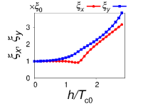
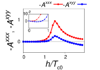
(e)

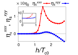
Figure 3: (a) The transition line ${T_{\rm c}}(h)$ of a $d$-wave Rashba-Zeeman superconductor, and (b) Cooper-pair momentum $-q_{0}$, (c) GL coherence length $\xi_{x},\xi_{y}$, (d) the asymmetry parameter $-{\mathcal{A}}^{xxx},-{\mathcal{A}}^{xyy}$, and (e) strength of rectification $\eta^{xxx}_{\rm{s}}$ and NHE $\eta^{xyy}_{\rm{s}}$ along the transition line $({T_{\rm c}}(h),h)$. Here, $T_{c}(h)$ and $q_{0}(h)$ are indicated by black disks. $\xi_{x}$, ${\mathcal{A}}^{xxx}$, $\eta_{\rm{s}}^{xxx}$ are indicated by red disks while $\xi_{y}$, ${\mathcal{A}}^{xyy}$, $\eta_{\rm{s}}^{xyy}$ by blue squares. The black, red, and blue lines are the guide for the eye.

Overall, the obtained anharmonicity parameters and NCT are of the same order in magnitude as those of the $s$-wave states in units of $\eta_{0}$. Thus, the enhanced NCT under moderate and strong magnetic fields is a general feature regardless of the pairing symmetry. The difference from the $s$-wave state is the behavior of $\eta_{\rm{s}}^{xxx}$ at high fields: The sign reversal of $\eta_{\rm{s}}^{xxx}$ seen in the $s$-wave state does not occur in the $d$-wave state for the range of $h/{T_{\rm c0}}$ shown here. We find a sign reversal for $h/{T_{\rm c0}}\lesssim 4$ [data not shown], but larger $L_{x}$ and $L_{y}$ are necessary to conclude its presence due to the large coherence lengths at low temperatures. It should also be noted that the quantum-fluctuation corrections may be important for such low temperatures.

(a)	(b)
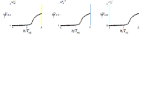
(c)	(d)

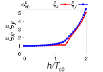
(e)

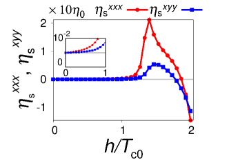
Figure 4: (a) The transition line ${T_{\rm c}}(h)$ of the $s$-wave Rashba-Zeeman superconductor with a high ${T_{\rm c0}}$, and (b) Cooper-pair momentum $-q_{0}$, (c) GL coherence length $\xi_{x},\xi_{y}$, (d) the asymmetry parameter $-{\mathcal{A}}^{xxx},-{\mathcal{A}}^{xyy}$, and (e) strength of rectification $\eta^{xxx}_{\rm{s}}$ and NHE $\eta^{xyy}_{\rm{s}}$ along the transition line $({T_{\rm c}}(h),h)$. Here, $T_{c}(h)$ and $q_{0}(h)$ are indicated by black disks. $\xi_{x}$, ${\mathcal{A}}^{xxx}$, $\eta_{\rm{s}}^{xxx}$ are indicated by red disks while $\xi_{y}$, ${\mathcal{A}}^{xyy}$, $\eta_{\rm{s}}^{xyy}$ by blue squares. The black, red, and blue lines are the guide for the eye.

(a)	(b)
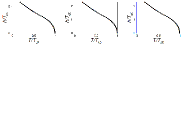
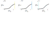
(c)	(d)

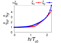
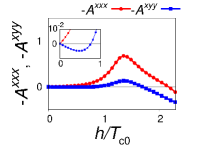
(e)

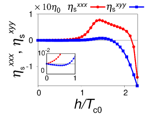
Figure 5: (a) The transition line ${T_{\rm c}}(h)$ of the $d$-wave Rashba-Zeeman superconductor with a high ${T_{\rm c0}}$, and (b) Cooper-pair momentum $-q_{0}$, (c) GL coherence length $\xi_{x},\xi_{y}$, (d) the asymmetry parameter $-{\mathcal{A}}^{xxx},-{\mathcal{A}}^{xyy}$, and (e) strength of rectification $\eta^{xxx}_{\rm{s}}$ and NHE $\eta^{xyy}_{\rm{s}}$ along the transition line $({T_{\rm c}}(h),h)$. Here, $T_{c}(h)$ and $q_{0}(h)$ are indicated by black disks. $\xi_{x}$, ${\mathcal{A}}^{xxx}$, $\eta_{\rm{s}}^{xxx}$ are indicated by red disks while $\xi_{y}$, ${\mathcal{A}}^{xyy}$, $\eta_{\rm{s}}^{xyy}$ by blue squares. The black, red, and blue lines are the guide for the eye.

To further study the quantitative aspects of NCT, we show the results for another parameter set

$$(t,\alpha_{\rm R},\mu,U_{s},U_{d}) =(1,0.3,-1,0.945,0.75),$$ (59)

in Figs. 4 and 5. The strength of the interaction $U_{s}$ and $U_{d}$ are chosen to give a high transition temperature ${T_{\rm c0}}\sim 0.1$ for both $s$- and $d$-wave states. We also choose a larger value of $\alpha_{\rm R}=0.3$ to ensure $\alpha_{\rm R}>{T_{\rm c0}}$. We used $L_{x}=6000$ and $L_{y}=500$ to determine ${T_{\rm c}}(h)$ and $q_{0}(h)$, while $L_{x}=6000$ and $L_{y}=4000$ are used to evaluate GL coefficients.

Qualitatively the same results are obtained for the strong-coupling superconductors, except for the behavior of $h/{T_{\rm c0}}\gtrsim 1$ in the $d$-wave states. The important point is that the enhanced NCT is obtained in the crossover region of strong-coupling superconductors as well. Furthermore, NCT is comparable to that of weak-coupling superconductors in units of $\eta_{0}$. Thus, it is established that the enhanced NCT is a universal property of the helical superconductivity regardless of ${T_{\rm c0}}$ when scaled with $\eta_{0}\sim\xi_{0}/{T_{\rm c0}}$.

III.1 Estimate of rectification and NHE

Let us make an order estimate of NCT obtained by the microscopic calculations. We start from the formula

$$-L_{z}^{-1}\eta^{ijk}_{{\rm{s}}} =\frac{\pi\sqrt{\xi_{x}\xi_{y}}}{T}\left(\frac{\xi_{x}\xi_{y}}{\xi_{j}\xi_{k}}\right)^{2}{\mathcal{A}}^{ijk}.$$ (60)

The numerical results are comparable in units of $\eta_{0}=L_{z}\xi_{0}/{T_{\rm c0}}$. Note that we have set the elementary charge $e$ and the Dirac constant $\hbar$ to unity in the derivation of the formula. Recovering $1=e{R_{\rm K}}/2\pi$ with

$${R_{\rm K}}\equiv\frac{2\pi\hbar}{e^{2}}\sim 2.6\times 10^{4}\ \Omega,$$ (61)

which is abbreviated in the formula, we obtain

$$\eta_{0}=L_{z}\frac{\xi_{0}}{{T_{\rm c0}}}\frac{e{R_{\rm K}}}{2\pi}\sim 5\times 10^{-5}\ \mathrm{\mu m^{2}/\mu A}\frac{L_{z}\xi_{0}/[\mathrm{nm}^{2}]}{{T_{\rm c0}}/[\mathrm{K}]}.$$ (62)

In the following, we estimate typical values of $\eta_{0}$ and thereby estimate NCT.

Let us assume a strongly-correlated superconductor $\xi_{0}\sim 5\ \mathrm{nm}$ and ${T_{\rm c0}}\sim 2\ \mathrm{K}$, which corresponds to CeCoIn₅ superlattices [66]. We also assume a sample thickness $L_{z}\sim{10}\ \mathrm{nm}$. These values lead to

$$\eta_{0} \sim{10^{-3}}\ \mathrm{\mu m^{2}/\mu A}.$$ (63)

Thus, we obtain $\eta_{\rm{s}}^{xxx}\sim 10\eta_{0}\sim{10^{-2}}\ \mathrm{\mu m^{2}/\mu A}$ and $\eta_{\rm{s}}^{xyy}\sim\eta_{0}\sim{10^{-3}}\ \mathrm{\mu m^{2}/\mu A}$.

To compare the obtained rectification with that expected from the parity-mixing mechanism [32], we focus on the MCA (i.e. $h$-linear rectification) by the anharmonicity parameter. In our calculation, MCA (multiplied by $h$) is obtained as $\eta^{xxx}_{\rm{s}}\sim 10^{-4}$ in units of $10\eta_{0}$, which is $10^{-4}$ times smaller than the rectification in the crossover region. According to Ref. [32], the ratio of MCA caused by the anharmonicity parameters to that by the parity-mixing mechanism is $\sim r_{t,s}(E_{F}/{T_{\rm c}})^{2}$, which is $O(10^{3})$ by assuming $E_{F}/{T_{\rm c}}\sim t/{T_{\rm c}}\sim 10^{2}$ and the ratio of spin-triplet to -singlet pairing glues $r_{t,s}\sim 0.1$ adopted in Ref. [32]. Thus, the presumable MCA which would be obtained when the parity mixing was taken into account in our model is smaller by one order in magnitude than the rectification by the helical-superconductivity crossover. Thus, the enhancement by the helical-superconductivity crossover is always visible and dominant even when the parity mixing is considered. Note also that the parity-mixing mechanism requires the odd-parity pairing interaction comparable to the even-parity one, which would not be satisfied in all the noncentrosymmetric superconductors.

We also estimate typical values for nonlinear resistivity by taking the linear resistivity of a heavy-fermion superlattice $\rho_{1{\rm{n}}}\sim 5\times 10^{-7}\ \Omega\mathrm{m}$ [66] as an example. For simplicity, we assume

$$\sigma^{xx}_{1{\rm{n}}}=\sigma^{yy}_{1{\rm{n}}}=\sigma_{1{\rm{n}}}=\rho_{1{\rm{n}}}^{-1}.$$ (64)

Neglecting the contribution of the normal-state nonlinear conductivity $\sigma_{2{\rm{n}}}^{ijk}$, the nonlinear resistivity at the reduced temperature $\epsilon$ is given by

$$\rho_{2}^{xii}(\epsilon) =-[\sigma^{-1}_{1}(\epsilon)]^{xa}\sigma_{2{\rm{s}}}^{abc}[\sigma^{-1}_{1}(\epsilon)]^{bi}[\sigma^{-1}_{1}(\epsilon)]^{ci}$$ (65)

$$=-\rho_{1{\rm{n}}}\left[\frac{\sigma_{1{\rm{n}}}}{\sigma_{1{\rm{n}}}+\sigma_{1{\rm{s}}}^{xx}(\epsilon)}\right]\left[\frac{\sigma_{1{\rm{s}}}^{ii}(\epsilon)}{\sigma_{1{\rm{n}}}+\sigma_{1{\rm{s}}}^{ii}(\epsilon)}\right]^{2}\eta^{xii}_{{\rm{s}}}$$

$$=-\left[1+\frac{\sigma^{xx}_{1{\rm{s}}}(\epsilon)}{\sigma_{1{\rm{n}}}}\right]^{-1}\left[{1+\frac{\sigma_{1{\rm{n}}}}{\sigma_{1{\rm{s}}}^{ii}(\epsilon)}}\right]^{-2}\rho_{1{\rm{n}}}\eta^{xii}_{{\rm{s}}}.$$

To obtain the second line, we used $\sigma^{xy}_{1}=0$ ensured due to the $y$-mirror plane and

$$\sigma_{2{\rm{s}}}^{xbc}(\epsilon)[\sigma^{-1}_{1{\rm{s}}}(\epsilon)]^{bi}[\sigma^{-1}_{1{\rm{s}}}(\epsilon)]^{ci}=\eta_{{\rm{s}}}^{xii}.$$ (66)

In the following, we evaluate rectification and NHE separately.

III.1.1 Rectification

To estimate the rectification in the fluctuation regime, let us consider the reduced temperature $\epsilon_{*}$ defined by

$$\frac{1}{3}\sigma_{1{\rm{n}}}=\sigma_{1{\rm{s}}}^{xx}(\epsilon_{*})=\frac{1}{L_{z}}\frac{\xi_{x}^{2}}{16\epsilon_{*}\xi_{x}\xi_{y}}.$$ (67)

The longitudinal resistivity is estimated to be

$$\rho^{xxx}_{2*} =-\frac{3}{4}\left(\frac{1}{4}\right)^{2}\rho_{1{\rm{n}}}\eta_{\rm{s}}^{xxx}\sim 10^{-4}\ {\rm\Omega\mu m^{3}/\mu A}.$$ (68)

Note that nonreciprocity at $\epsilon=\epsilon_{*}$,

$$\eta_{*}^{xxx}=\left[{1+\frac{\sigma_{1{\rm{n}}}}{\sigma_{1{\rm{s}}}^{xx}(\epsilon_{*})}}\right]^{-2}\eta^{xxx}_{{\rm{s}}}=\frac{1}{16}\eta_{{\rm{s}}}^{xxx},$$ (69)

is smaller than $\eta_{{\rm{s}}}^{xxx}$ since $\epsilon_{*}$ is larger than $\epsilon=0$. This is estimated to be

$$\eta_{*}^{xxx}\sim 10^{-3}\ {\rm\mu m^{2}/\mu A}.$$ (70)

III.1.2 NHE

To estimate NHE in the fluctuation regime, let us consider $\epsilon_{*}$ defined by

$$\frac{1}{3}\sigma_{1{\rm{n}}}=\sigma_{1{\rm{s}}}^{yy}(\epsilon_{*}),$$ (71)

instead of Eq. (67). This corresponds to the $25\%$ drop of the longitudinal resistance under concern, i.e. the applied electric current in the $y$ direction. The transverse resistivity $\rho_{2}^{xyy}$ is then given by

$$\rho^{xyy}_{2*} =-\left[1+\frac{1}{3}\frac{\sigma_{1{\rm{s}}}^{xx}(\epsilon_{*})}{\sigma_{1{\rm{s}}}^{yy}(\epsilon_{*})}\right]^{-1}\left(\frac{1}{4}\right)^{2}\rho_{1{\rm{n}}}\eta_{\rm{s}}^{xyy}$$

$$\sim 10^{-5}\ {\rm\Omega\mu m^{3}/\mu A},$$ (72)

by using

$$\frac{\sigma^{xx}_{1{\rm{s}}}(\epsilon)}{\sigma^{yy}_{1{\rm{s}}}(\epsilon)} =\frac{\xi_{x}^{2}}{\xi_{y}^{2}}\sim\frac{1}{4},$$ (73)

for the crossover region.

IV Derivation of the general formula for the nonlinear fluctuation conductivity

In the following, we derive the formula of the nonlinear fluctuation conductivity represented by the eigenstates and eigenvalues of the GL coefficient ${\hat{\alpha}}$. We consider the GL free-energy functional of the form

$$F[\ket{\psi}] =V\braket{\psi}{{\hat{\alpha}}}{\psi}.$$ (74)

Here, the GL coefficient operator ${\hat{\alpha}}$ is arbitrary: For example, it can include both $\bm{x}$ and $\nabla/i$ in the presence of the orbital magnetic field, while is a matrix when the system has several pairing channels. Accordingly, the phenomenological TDGL equation is given by

$$\Gamma_{0}\partial_{t}\ket{\psi(t)} =-{\hat{\alpha}}(t)\ket{\psi(t)}+\ket{\zeta(t)},$$ (75)

which recasts into the standard expression by $\psi_{\bm{q}}(t)=\braket{\bm{q}}{\psi(t)}$ and so on. The electric field is incorporated into ${\hat{\alpha}}(t)$ by the vector potential $A_{i}(t)=-E_{i}t$. We assume $\Gamma_{0}>0$ for simplicity and set $\Gamma_{0}\to 1$ in the following. $\Gamma_{0}$ will be recovered by $\hat{\alpha}\to\hat{\alpha}/\Gamma_{0}$ at the end of the calculation. The random force $\ket{\zeta(t)}$ satisfies

$$\ket{\zeta(t)}\bra{\zeta(t^{\prime})}\to\frac{2}{\beta V}\delta(t-t^{\prime})\hat{1},$$ (76)

after taking the noise average. The identity operator $\hat{1}$ is abbreviated in the following. We also abbreviate the subscript “s” representing the paraconductivity contribution in the following for simplicity.

We are interested in the electric current carried by the steady-state solution of the TDGL equation,

$$\ket{\psi(t)} =\int_{0}^{\infty}dt^{\prime}\,U(t,t-t^{\prime})\ket{\zeta(t-t^{\prime})},$$ (77)

where the time-evolution operator is given by

$$U(t,t-t^{\prime})\equiv T\exp\left(-\int_{t-t^{\prime}}^{t}d\tau\,{\hat{\alpha}}(\tau)\right).$$ (78)

Note that we can write

$${\hat{\alpha}}(t)=U_{\chi}(t){\hat{\alpha}}U_{\chi}(t)^{\dagger},$$ (79)

with ${\hat{\alpha}}\equiv{\hat{\alpha}}(0)$ and the unitary operator $U_{\chi}(t)$ representing the gauge transform. Thus, we obtain $U(t,t-t^{\prime})=U_{\chi}(t)U(0,-t^{\prime})U_{\chi}(t)^{\dagger}$ and

$$\ket{\psi(t)}=U_{\chi}(t)\int_{0}^{\infty}dt^{\prime}\,U(0,-t^{\prime})U_{\chi}(t)^{\dagger}\ket{\zeta(t-t^{\prime})}.$$ (80)

The electric-current operator at the time $t$ is given by

$$j_{i}(t)\equiv-\partial_{A_{i}}{\hat{\alpha}}(t)=U_{\chi}(t)j_{i}U_{\chi}(t)^{\dagger}.$$ (81)

Thus, the electric current is given by

$$\braket{j_{i}(t)} \equiv\braket{\psi(t)}{j_{i}(t)}{\psi(t)}$$

$$={\int_{0}^{\infty}}dt_{1}{\int_{0}^{\infty}}dt_{2}\,\mathrm{Tr}\,[U_{\chi}(t)^{\dagger}\ket{\zeta(t-t_{2})}$$

$$\quad\cdot\bra{\zeta(t-t_{1})}U_{\chi}(t)U(0,-t_{1})^{\dagger}j_{i}U(0,-t_{2})]$$

$$\to\frac{2}{\beta V}{\int_{0}^{\infty}}ds\,\mathrm{Re}\mathrm{Tr}\,[j_{i}U(s)e^{-2{\hat{\alpha}}s}U(s)^{\dagger}],$$ (82)

which is independent of $t$ owing to the balance of the applied electric field and the relaxation process. Here we took the noise average to obtain the last line, defining

$$U(s)\equiv\,T\exp\left(-\int^{0}_{-s}d\tau\,{\hat{\alpha}}(\tau)\right)e^{{\hat{\alpha}}s},$$ (83)

which represents the deviation of the time evolution under the electric field from the one in the absence of the field.

The nonlinear fluctuation conductivity is obtained by expanding $U(s)$ in terms of the electric field. For this purpose, let us define

$$\delta{\hat{\alpha}}(t)\equiv{\hat{\alpha}}(t)-{\hat{\alpha}},\quad\mathcal{E}(t)\equiv-e^{-{\hat{\alpha}}t}\delta{\hat{\alpha}}(-t)e^{{\hat{\alpha}}t}.$$ (84)

The operator $\mathcal{E}(t)$ can be expanded by the electric field as $\mathcal{E}(t)=\sum_{n=1}^{\infty}\mathcal{E}_{n}(t)$ with $\mathcal{E}_{n}(t)=O(E^{n})$. The first two terms are given by

$$\mathcal{E}_{1}(t) =-A_{j}(-t)e^{-{\hat{\alpha}}t}\partial_{A_{j}}\delta{\hat{\alpha}}(-t)e^{{\hat{\alpha}}t}$$

$$=t\,E_{j}e^{-{\hat{\alpha}}t}j_{j}e^{{\hat{\alpha}}t},$$ (85a)

$$\mathcal{E}_{2}(t) =\frac{t^{2}}{2}E_{j}E_{k}\,e^{-{\hat{\alpha}}t}\partial_{A_{j}}j_{k}e^{{\hat{\alpha}}t}.$$ (85b)

Since $U(s)$ satisfies

$$\partial_{s}U(s) =U(s)\mathcal{E}(s),$$ (86)

we obtain the integral equation

$$U(s) =1+\int_{0}^{s}dt_{1}\,U(t_{1})\mathcal{E}(t_{1})$$

$$=1+\int_{0}^{s}dt_{1}\,\mathcal{E}(t_{1})$$

$$\quad+\int_{0}^{s}dt_{1}\int^{t_{1}}_{0}dt_{2}\,\mathcal{E}(t_{2})\mathcal{E}(t_{1})+O(E^{3}).$$ (87)

Thus, the electric current of $O(E^{n})$ ($n=0,1,2$) is obtained by $\delta^{n}j_{i}$ as follows. The zero-th order term vanishes,

$$\delta^{0}j_{i} =\frac{2}{\beta V}\int_{0}^{\infty}ds\,\mathrm{Re}\mathrm{Tr}\,[j_{i}e^{-2{\hat{\alpha}}s}]$$

$$=-\frac{2}{\beta V}\int_{0}^{\infty}ds\,\frac{1}{2s}\partial_{A_{i}}\mathrm{Re}\mathrm{Tr}\,[e^{-2{\hat{\alpha}}s}]$$

$$=0,$$ (88)

according to the gauge invariance. The first-order electric current is given by

$$\delta^{1}j_{i} =\frac{4}{\beta V}\int_{0}^{\infty}ds\int_{0}^{s}dt_{1}\,\mathrm{Re}\mathrm{Tr}\,[j_{i}\mathcal{E}_{1}(t_{1})e^{-2{\hat{\alpha}}s}].$$ (89)

It is easy to see that $\delta^{1}j_{i}=\sigma_{1}^{ij}E_{j}$ gives

$$\sigma_{1}^{ij}=\frac{\Gamma_{0}}{\beta V}\sum_{\mu\nu}\frac{\mathrm{Re}[\braket{\mu}{j_{i}}{\nu}\braket{\nu}{j_{j}}{\mu}]}{\alpha_{\mu}\alpha_{\nu}(\alpha_{\mu}+\alpha_{\nu})},$$ (90)

which reproduces the formulas in Refs. [77, 69] as well as Eq. (32) by $j_{i}\to 2\partial_{q_{i}}\alpha_{\bm{q}}$. Here and hereafter, we use the notation ${\hat{\alpha}}\ket{\mu}=\alpha_{\mu}\ket{\mu}.$

The second-order electric current consists of three terms,

$$\delta^{2}j_{i} =\delta^{2}_{a}j_{i}+\delta^{2}_{b}j_{i}+\delta^{2}_{c}j_{i},$$ (91)

where $\delta^{2}_{a}j_{i}$ is given by

$$\delta^{2}_{a}j_{i} =\frac{4}{\beta V}\int_{0}^{\infty}ds\int_{0}^{s}dt_{1}\,\mathrm{Re}\mathrm{Tr}\,[j_{i}\mathcal{E}_{2}(t_{1})e^{-2{\hat{\alpha}}s}]$$

$$=\frac{4}{\beta V}{\int_{0}^{\infty}}dt_{1}\int_{t_{1}}^{\infty}ds\,\mathrm{Re}\mathrm{Tr}\,[j_{i}\mathcal{E}_{2}(t_{1})e^{-2{\hat{\alpha}}s}],$$ (92)

for example. After similar procedures, we obtain

$$\delta^{2}_{a}j_{i} =\frac{4}{\beta V}{\int_{0}^{\infty}}dt_{1}\int_{0}^{\infty}ds\,\mathrm{Re}\mathrm{Tr}\,[j_{i}\mathcal{E}_{2}(t_{1})e^{-2{\hat{\alpha}}(s+t_{1})}],$$ (93a)

$$\delta^{2}_{b}j_{i} =\frac{4}{\beta V}\int_{0}^{\infty}dt_{2}\int_{0}^{\infty}dt_{1}\int_{0}^{\infty}ds\,\mathrm{Re}\mathrm{Tr}\,[j_{i}\mathcal{E}_{1}(t_{1}+t_{2})e^{-2{\hat{\alpha}}(s+t_{1}+t_{2})}\mathcal{E}_{1}(t_{2})^{\dagger}],$$ (93b)

$$\delta^{2}_{c}j_{i} =\frac{4}{\beta V}{\int_{0}^{\infty}}dt_{2}\int_{0}^{\infty}dt_{1}\int_{0}^{\infty}ds\,\mathrm{Re}\mathrm{Tr}\,[j_{i}\mathcal{E}_{1}(t_{2})\mathcal{E}_{1}(t_{1}+t_{2})e^{-2{\hat{\alpha}}(s+t_{1}+t_{2})}].$$ (93c)

Before proceeding, we erase $\partial_{A_{j}}j_{k}$ from the expression of $\delta_{a}^{2}j_{i}$. Let us consider an auxiliary quantity

$$T_{i} \equiv\mathrm{Re}\mathrm{Tr}\,[\partial_{A_{i}}j_{j}e^{-{\hat{\alpha}}t_{1}}j_{k}e^{-{\hat{\alpha}}(2s+t_{1})}]E_{j}E_{k}$$

$$=2\partial_{A_{i}}T_{0}-\mathrm{Re}\mathrm{Tr}\,[j_{j}\partial_{A_{i}}(e^{-{\hat{\alpha}}t_{1}})j_{k}e^{-{\hat{\alpha}}(2s+t_{1})}]E_{j}E_{k}$$

$$\qquad-\mathrm{Re}\mathrm{Tr}\,[j_{j}e^{-{\hat{\alpha}}t_{1}}j_{k}\partial_{A_{i}}(e^{-{\hat{\alpha}}(2s+t_{1})})]E_{j}E_{k}$$

$$\qquad-\mathrm{Re}\mathrm{Tr}\,[j_{j}e^{-{\hat{\alpha}}t_{1}}\partial_{A_{i}}j_{k}e^{-{\hat{\alpha}}(2s+t_{1})}]E_{j}E_{k},$$ (94)

with $2T_{0}\equiv\mathrm{Re}\mathrm{Tr}\,[j_{j}e^{-{\hat{\alpha}}t_{1}}j_{k}e^{-{\hat{\alpha}}(2s+t_{1})}]E_{j}E_{k}$. The last line is equivalent to $-T_{i}$ by interchanging the dummy variables $j$ and $k$. We also obtain

$$\partial_{A_{i}}e^{-{\hat{\alpha}}t_{1}} =\int_{0}^{1}d\theta\,e^{-\theta{\hat{\alpha}}t}\partial_{A_{i}}(-{\hat{\alpha}}t_{1})e^{{\hat{\alpha}}t_{1}(1-\theta)}$$

$$=\int_{0}^{t_{1}}dt_{2}\,e^{-{\hat{\alpha}}t_{2}}j_{i}e^{-{\hat{\alpha}}(t_{1}-t_{2})},$$ (95a)

$$\partial_{A_{i}}e^{-{\hat{\alpha}}(2s+t_{1})} =\partial_{A_{i}}(e^{-{\hat{\alpha}}2s})e^{-{\hat{\alpha}}t_{1}}+e^{-2s{\hat{\alpha}}}\partial_{A_{i}}(e^{-{\hat{\alpha}}t_{1}})$$

$$=2\int_{0}^{s}dt_{2}\,e^{-{\hat{\alpha}}2t_{2}}j_{i}e^{-{\hat{\alpha}}[2(s-t_{2})+t_{1}]}$$

$$\quad+\int_{0}^{t_{1}}dt_{2}\,e^{-{\hat{\alpha}}(2s+t_{2})}j_{i}e^{-{\hat{\alpha}}(t_{1}-t_{2})}.$$ (95b)

Thus, we obtain

$$T_{i} =\partial_{A_{i}}T_{0}-\frac{1}{2}\int_{0}^{t_{1}}dt_{2}\,[f_{i}(t_{2},t_{1}-t_{2},2s+t_{1})$$

$$\qquad+f_{i}(2s+t_{2},t_{1}-t_{2},t_{1})]$$

$$\qquad-\int_{0}^{s}dt_{2}\,f_{i}(2t_{2},2(s-t_{2})+t_{1},t_{1}),$$ (96)

with

$$f_{i}(t_{a},t_{b},{T_{\rm c}}) \equiv\mathrm{Re}\mathrm{Tr}\,[e^{-{\hat{\alpha}}t_{a}}j_{i}e^{-{\hat{\alpha}}t_{b}}j_{j}e^{-{\hat{\alpha}}{T_{\rm c}}}j_{k}]E_{j}E_{k}$$

$$=f_{i}(t_{b},t_{a},{T_{\rm c}}).$$ (97)

The integrand of $\delta^{2}_{a}j_{i}$ is, by using $\partial_{A_{j}}j_{i}=\partial_{A_{i}}j_{j}$,

$$\mathrm{Re}\mathrm{Tr}\,[j_{i}\mathcal{E}_{2}(t_{1})e^{-{\hat{\alpha}}2(s+t_{1})}]$$

$$=\frac{t_{1}^{2}}{2}\mathrm{Re}\mathrm{Tr}\,[j_{i}e^{-{\hat{\alpha}}t_{1}}\partial_{A_{j}}j_{k}e^{-{\hat{\alpha}}(2s+t_{1})}]E_{j}E_{k}$$

$$=E_{j}\partial_{A_{j}}S_{i}-\frac{t_{1}^{2}}{2}T_{i}$$ (98)

$$\qquad-\frac{t_{1}^{2}}{2}\mathrm{Re}\mathrm{Tr}\,[j_{i}\partial_{A_{j}}(e^{-{\hat{\alpha}}t_{1}})j_{k}e^{-{\hat{\alpha}}(2s-t_{1})}]E_{j}E_{k}$$

$$\qquad-\frac{t_{1}^{2}}{2}\mathrm{Re}\mathrm{Tr}\,[j_{i}e^{-{\hat{\alpha}}t_{1}}j_{k}\partial_{A_{j}}(e^{-{\hat{\alpha}}(2s-t_{1})})]E_{j}E_{k},$$

with $S_{i}\equiv(t_{1}^{2}/2)\mathrm{Re}\mathrm{Tr}\,[j_{i}e^{-{\hat{\alpha}}t_{1}}j_{k}e^{-{\hat{\alpha}}(2s+t_{1})}]E_{k}$. The total derivatives of the vector potential $E_{j}\partial_{A_{j}}S_{i}$ and $\partial_{A_{i}}T_{0}$ vanish according to the gauge invariance. Thus, we obtain after changing the integral variables,

$$\delta^{2}_{a}j_{i} =\frac{2}{\beta V}\iiint_{t_{1},t_{2},s}\left[(t_{1}+t_{2})^{2}a_{1}^{i}(t_{1}+t_{2},t_{2},s)\right.$$

$$\qquad\left.+t_{1}^{2}a_{2}^{i}(t_{1},t_{2},s+t_{2})\right],$$ (99)

with

$$\iiint_{t_{1},t_{2},s}\equiv{\int_{0}^{\infty}}dt_{1}{\int_{0}^{\infty}}dt_{2}{\int_{0}^{\infty}}ds,$$ (100)

and

$$a_{1}^{i}(t_{1}+t_{2},t_{2},s) =\frac{1}{2}[f_{i}(t_{2},t_{1},2s+t_{1}+t_{2})+f_{i}(2s+t_{2},t_{1},t_{1}+t_{2})]$$

$$\quad-f_{i}(2s+t_{1}+t_{2},t_{2},t_{1})-f_{i}(t_{1},t_{1}+t_{2},2s+t_{2}),$$ (101a)

$$a_{2}^{i}(t_{1},t_{2},s+t_{2}) =f_{i}(2t_{2},2s+t_{1},t_{1})-2f_{i}(2s+t_{1},t_{1},2t_{2}).$$ (101b)

We also obtain

$$\delta^{2}_{b}j_{i} =\frac{2}{\beta V}\iiint_{t_{1},t_{2},s}\,2t_{1}(t_{1}+t_{2})f_{i}(t_{1},t_{1}+t_{2},2s+t_{2}),$$ (102a)

$$\delta^{2}_{c}j_{i} =\frac{2}{\beta V}\iiint_{t_{1},t_{2},s}2t_{2}(t_{1}+t_{2})f_{i}(2s+t_{1}+t_{2},t_{2},t_{1}).$$ (102b)

Combining these terms, the second-order electric current $\delta^{2}j_{i}$ is obtained by

$$\delta^{2}j_{i} =u_{i}+v_{i}+w_{i},$$ (103)

with

$$u_{i} \equiv\frac{2}{\beta V}\iiint_{t_{1},t_{2},s}\frac{1}{2}(t_{1}+t_{2})^{2}[f_{i}(t_{2},t_{1},2s+t_{1}+t_{2})$$

$$\qquad\quad+f_{i}(2s+t_{2},t_{1},t_{1}+t_{2})],$$ (104a)

$$v_{i} \equiv\frac{2}{\beta V}\iiint_{t_{1},t_{2},t_{3}}t_{1}^{2}[f_{i}(2s+t_{1},2t_{2},t_{1})$$

$$\qquad\quad-2f_{i}(2s+t_{1},t_{1},2t_{2})],$$ (104b)

$$w_{i} \equiv\frac{2}{\beta V}\iiint_{t_{1},t_{2},s}(t_{1}^{2}-t_{2}^{2})[f_{i}(t_{1},t_{1}+t_{2},2s+t_{2})$$

$$\qquad-f_{i}(2s+t_{1}+t_{2},t_{2},t_{1})].$$ (104c)

Now, the integrals can be straightforwardly performed as the products of gamma functions, by introducing the current matrix element by

$$J_{\mu\nu\lambda}^{i} \equiv\mathrm{Re}[\braket{\mu}{j_{i}}{\nu}\braket{\nu}{j_{j}}{\lambda}\braket{\lambda}{j_{k}}{\mu}]E_{j}E_{k}$$

$$=J^{i}_{\nu\mu\lambda},$$ (105)

as well as expanding $f_{i}$ by

$$f_{i}(t_{a},t_{b},{T_{\rm c}})=\sum_{\mu\nu\lambda}J^{i}_{\mu\nu\lambda}e^{-(\alpha_{\mu}t_{a}+\alpha_{\nu}t_{b}+\alpha_{\lambda}{T_{\rm c}})}.$$ (106)

The results are

$$u_{i} =\frac{2}{\beta V}\sum_{\mu\nu\lambda}\frac{J^{i}_{\mu\nu\lambda}}{2\alpha_{\mu}\alpha_{\lambda}(\alpha_{\nu}+\alpha_{\lambda})}\left(\frac{1}{(\alpha_{\nu}+\alpha_{\lambda})^{2}}+\frac{1}{(\alpha_{\nu}+\alpha_{\lambda})(\alpha_{\mu}+\alpha_{\lambda})}+\frac{1}{(\alpha_{\mu}+\alpha_{\lambda})^{2}}\right),$$ (107a)

$$v_{i} =\frac{2}{\beta V}\sum_{\mu\nu\lambda}\frac{J^{i}_{\mu\nu\lambda}}{2\alpha_{\mu}}\left(\frac{1}{\alpha_{\nu}(\alpha_{\mu}+\alpha_{\lambda})^{3}}-\frac{2}{\alpha_{\lambda}(\alpha_{\mu}+\alpha_{\nu})^{3}}\right),$$ (107b)

$$w_{i} =\frac{2}{\beta V}\sum_{\mu\nu\lambda}\frac{J^{i}_{\mu\nu\lambda}}{\alpha_{\nu}\alpha_{\lambda}(\alpha_{\mu}+\alpha_{\nu})}\left(\frac{1}{(\alpha_{\mu}+\alpha_{\nu})^{2}}-\frac{1}{(\alpha_{\nu}+\alpha_{\lambda})^{2}}\right).$$ (107c)

Summing up these terms, we finally obtain the formula

$$\!\!\!\!\delta^{2}j_{i} =\frac{2}{\beta V}\sum_{\mu\nu\lambda}\frac{J^{i}_{\mu\nu\lambda}(\alpha_{\mu}+\alpha_{\nu}+2\alpha_{\lambda})}{\alpha_{\lambda}(\alpha_{\mu}+\alpha_{\nu})(\alpha_{\mu}+\alpha_{\lambda})^{2}(\alpha_{\nu}+\alpha_{\lambda})^{2}},$$ (108)

after symmetrizing the summand with respect to $\mu$ and $\nu$ by employing Mathematica. The formula in the main text is obtained by $\alpha,j_{i}\to\alpha/\Gamma_{0},j_{i}/\Gamma_{0}$ and so on. Note that Eq. (108) reproduces Eq. (37), since

$$\delta^{2}j_{i}\to\frac{2}{\beta V}\sum_{q}\frac{\partial_{q_{i}}\alpha_{\bm{q}}\partial_{q_{j}}\alpha_{\bm{q}}\partial_{q_{j}}\alpha_{\bm{q}}}{\alpha^{5}_{\bm{q}}}E_{j}E_{k},$$ (109)

by $J^{i}_{\mu\nu\lambda}\to 8\partial_{q_{i}}\alpha_{\bm{q}}\partial_{q_{j}}\alpha_{\bm{q}}\partial_{q_{j}}\alpha_{\bm{q}}$.

V Effect of the orbital magnetic field on nonreciprocal transport

Here we study the effect of the orbital magnetic field. We consider the GL coefficient

$${\hat{\alpha}} =[\alpha_{\bm{q}_{0}}+\alpha_{2}^{ij}\delta q_{i}\delta q_{j}+\alpha_{3}^{ijk}\delta q_{i}\delta q_{j}\delta q_{k}]_{\bm{q}\to\frac{\nabla}{i}-2\bm{A}(\bm{x})}$$ (110)

$$=N_{0}\left[\epsilon+\sum_{i}\xi_{i}^{2}P_{i}^{2}+\sum_{ijk}a_{3}^{ijk}(\xi_{i}P_{i})(\xi_{j}P_{j})(\xi_{k}P_{k})\right].$$

Here, we defined the operator

$$\bm{P} \equiv\frac{\nabla}{i}-\bm{q}_{0}-2\bm{A}(\bm{x}).$$ (111)

The vector potential $\bm{A}(\bm{x})$ represents the magnetic field in the $y$ direction. We rescale the coordinates by $x_{i}\to{\bar{x}}_{i}=x_{i}/\xi_{i}$, and thus

$${\mathcal{P}}_{i} \equiv\xi_{i}P_{i}=\frac{1}{i}\partial_{{\bar{x}}_{i}}-2{\mathcal{A}}_{i}(\bm{{\bar{x}}}),$$ (112)

with

$${\mathcal{A}}_{i}(\bm{{\bar{x}}})\equiv\xi_{i}q_{0i}/2+\delta_{ix}{\mathcal{B}}{\bar{z}},\quad{\mathcal{B}}\equiv B\xi_{x}\xi_{z}.$$ (113)

Thus, we focus on

$${\hat{\alpha}} =N_{0}\left[\epsilon+\bm{{\mathcal{P}}}^{2}+a_{3}^{ijk}{\mathcal{P}}_{i}{\mathcal{P}}_{j}{\mathcal{P}}_{k}\right].$$ (114)

${\hat{\alpha}}$ commutes with ${\mathcal{P}}_{y}$ and ${\mathcal{P}}_{x}$, and

$$[{\mathcal{P}}_{z},{\mathcal{P}}_{x}]=2i{\mathcal{B}}.$$ (115)

The system volume in the $\bm{{\bar{x}}}$ coordinates is given by $\bar{V}\equiv\bar{L}_{x}\bar{L}_{y}\bar{L}_{z}$ with $\bar{L}_{i}\equiv L_{i}/\xi_{i}$. Since we are interested in the first-order effect of $a_{3}^{ijk}$, we can consider each component of $a_{3}^{ijk}$ separately. In the following, we set $N_{0}\to 1$, which will be recovered at the end of the calculation.

V.1 Effect of $a_{3}^{xyy}$

We first consider the situation where only $a_{3}^{xyy}=a_{3}^{yxy}=a_{3}^{yyx}$ is finite. We have

$${\hat{\alpha}} =\epsilon+({\mathcal{P}}_{x}+3a_{3}^{xyy}{\mathcal{P}}_{y}^{2}/2)^{2}+{\mathcal{P}}_{y}^{2}+{\mathcal{P}}_{z}^{2},$$ (116)

up to $O(a_{3})$. Thus, ${\hat{\alpha}}$ is diagonalized by the Landau levels as well as the plane wave in the ${\bar{y}}$ direction. The annihilation operator is given by

$$a\equiv\frac{1}{\sqrt{4|{\mathcal{B}}|}}[{\mathcal{P}}_{z}+i\,\mathrm{sgn}\,[{\mathcal{B}}]({\mathcal{P}}_{x}+3a_{3}^{xyy}{\mathcal{P}}_{y}^{2}/2)],$$ (117)

and we obtain

$${\hat{\alpha}} =\epsilon+{\mathcal{P}}_{y}^{2}+4|{\mathcal{B}}|(a^{\dagger}a+1/2)$$

$$=\bar{\epsilon}+{\mathcal{P}}_{y}^{2}+4|{\mathcal{B}}|a^{\dagger}a,$$ (118)

with $\bar{\epsilon}\equiv\epsilon+2|{\mathcal{B}}|$. Here, $m$-th Landau level has the eigenvalue

$$\alpha_{m}(p_{y})={\bar{\epsilon}}+p_{y}^{2}+4|{\mathcal{B}}|m,$$ (119)

where $p_{y}$ and $m$ are the eigenvalues of ${\mathcal{P}}_{y}$ and $a^{\dagger}a$, respectively, and has the degeneracy

$$g=\frac{|{\mathcal{B}}|\bar{L}_{x}\bar{L}_{z}}{\pi}.$$ (120)

The electric current operator is given by

$$j_{x} =2\xi_{x}\partial_{{\mathcal{P}}_{x}}{\hat{\alpha}}$$

$$=4i\xi_{x}\mathrm{sgn}\,[{\mathcal{B}}]\sqrt{|{\mathcal{B}}|}(a^{\dagger}-a),$$ (121a)

$$j_{y}+\delta j_{y} \equiv 2\xi_{y}\partial_{{\mathcal{P}}_{y}}{\hat{\alpha}}$$

$$=4\xi_{y}{\mathcal{P}}_{y}\left(1+\frac{3a_{3}^{xyy}}{4\xi_{x}}j_{x}\right),$$ (121b)

and thus their matrix elements between Landau levels $a^{\dagger}a\ket{n}=n\ket{n}$ are obtained by

$$|\braket{m}{j_{x}}{n}|^{2} =16\xi_{x}^{2}|{\mathcal{B}}|(m\delta_{m,n+1}+n\delta_{m+1,n}),$$ (122a)

$$\braket{m}{\delta j_{y}}{n} =4\xi_{y}{\mathcal{P}}_{y}\frac{3a_{3}^{xyy}}{4\xi_{x}}\braket{m}{j_{x}}{n}.$$ (122b)

In this case, only $\sigma_{2}^{xyy}$ and $\sigma_{2}^{yxy}=\sigma_{2}^{yyx}$can be finite: Indeed, $\sigma_{2}^{ijk}$ is not affected by $\alpha_{3}^{xyy}$ when neither of $i,j,k$ is $y$, while vanishes when either one or three of $i,j,k$ is $y$ according to the $y$ mirror plane. $\sigma^{ijk}_{2}$ with $\set{i,j,k}=\set{z,y,y}$ also vanishes by considering the matrix element (e.g., $\mathrm{Re}[\braket{m}{j_{x}}{n}\braket{n}{j_{z}}{m}]=0$). We obtain with $p_{y}$ the eigenvalue of ${\mathcal{P}}_{y}$,

$$\delta M_{\mu\nu\lambda}^{xyy} \equiv\mathrm{Re}[\braket{\mu}{j_{x}}{\nu}\braket{\nu}{\delta j_{y}}{\lambda}\braket{\lambda}{j_{y}}{\mu}]]$$

$$=16\xi_{y}^{2}\frac{3a_{3}^{xyy}}{4\xi_{x}}p_{y}^{2}\delta_{lm}|\braket{m}{j_{x}}{n}|^{2},$$ (123)

for $\mu=(m,p_{y})$, $\nu=(n,p_{y})$ and $\lambda=(l,p_{y})$ [Here and hereafter, the indices distinguishing degenerate Landau levels are abbreviated for simplicity]. The matrix element is thus given by

$$J^{xyy}_{\mu\nu\lambda} \equiv\mathrm{Re}[\braket{\mu}{j_{x}}{\nu}\braket{\nu}{(j_{y}+\delta j_{y})}{\lambda}\braket{\lambda}{(j_{y}+\delta j_{y})}{\mu}]$$

$$=J^{xyy}_{\mu\nu\lambda}|_{a_{3}\to 0}+\delta M_{\mu\nu\lambda}^{xyy}+\delta M_{\nu\mu\lambda}^{xyy}+O(a_{3}^{2}),$$ (124a)

$$J^{yyx}_{\mu\nu\lambda} =J^{xyy}_{\nu\lambda\mu}.$$ (124b)

Thus, we obtain up to $O(a_{3})$,

$$\sigma_{2}^{xyy} =\frac{2g}{\beta V}\sum_{\mu\nu\lambda}\frac{[\delta M_{\mu\nu\lambda}^{xyy}+\delta M_{\nu\mu\lambda}^{xyy}](\alpha_{\mu}+\alpha_{\nu}+2\alpha_{\lambda})}{\alpha_{\lambda}(\alpha_{\mu}+\alpha_{\nu})(\alpha_{\mu}+\alpha_{\lambda})^{2}(\alpha_{\nu}+\alpha_{\lambda})^{2}}$$

$$=\frac{4g}{\beta V}\sum_{p_{y}nml}\frac{\delta M_{\mu\nu\lambda}^{xyy}[3\alpha_{m}(p_{y})+\alpha_{n}(p_{y})]}{4\alpha_{m}^{3}(p_{y})[\alpha_{m}(p_{y})+\alpha_{n}(p_{y})]^{3}}.$$ (125)

The leading order term in ${\bar{\epsilon}}\propto\alpha_{0}(p_{y}=0)$ comes from $m=0$. Thus, we obtain

$$\sigma_{2}^{xyy} \sim\frac{4g}{\beta V}\sum_{p_{y}}\frac{16\xi_{y}^{2}\frac{3a_{3}^{xyy}}{4\xi_{x}}p_{y}^{2}\,16\xi_{x}^{2}|{\mathcal{B}}|}{4\alpha_{0}^{3}(p_{y})[\alpha_{0}(p_{y})+\alpha_{1}(p_{y})]^{2}}$$

$$=C^{xyy}\int\frac{dp_{y}}{2\pi}\frac{p_{y}^{2}}{(\bar{\epsilon}+p_{y}^{2})^{3}[\bar{\epsilon}+p_{y}^{2}+2|{\mathcal{B}}|]^{2}}$$

$$\sim C^{xyy}{\frac{1}{64{\mathcal{B}}^{2}\bar{\epsilon}^{3/2}}.}$$ (126)

The coefficient is

$$C^{xyy} =\frac{g}{\beta V}{\bar{L}_{y}}16\xi_{y}^{2}\frac{3a_{3}^{xyy}\,16\xi_{x}^{2}|{\mathcal{B}}|}{4\xi_{x}}\frac{1}{4}$$

$$=\frac{48{\mathcal{B}}^{2}}{\pi\beta\xi_{x}\xi_{y}\xi_{z}}[\xi_{x}\xi_{y}^{2}a_{3}^{xyy}].$$ (127)

Thus, we obtain

$$\sigma_{2}^{xyy} \sim\tau_{0}^{2}\frac{48{\mathcal{B}}^{2}}{\pi\beta\xi_{x}\xi_{y}\xi_{z}}[\xi_{x}\xi_{y}^{2}a_{3}^{xyy}]{\frac{1}{64{\mathcal{B}}^{2}\bar{\epsilon}^{3/2}}}$$

$$={\frac{3\tau_{0}^{2}T}{4\pi\bar{\epsilon}^{3/2}}{\mathcal{A}}^{xyy}.}$$ (128)

Here we recovered $\Gamma_{0}/N_{0}=\tau_{0}$.

Similarly, we obtain from Eq. (124b),

$$\sigma_{2}^{yyx} =\frac{2g}{\beta V}\sum_{\mu\nu\lambda}\frac{[\delta M_{\nu\lambda\mu}^{xyy}+\delta M_{\lambda\nu\mu}^{xyy}](\alpha_{\mu}+\alpha_{\nu}+2\alpha_{\lambda})}{\alpha_{\lambda}(\alpha_{\mu}+\alpha_{\nu})(\alpha_{\mu}+\alpha_{\lambda})^{2}(\alpha_{\nu}+\alpha_{\lambda})^{2}}$$

$$=\frac{2g}{\beta V}\sum_{\mu\nu\lambda}\frac{\delta M_{\mu\nu\lambda}^{xyy}(2\alpha_{\mu}+2\alpha_{\nu})}{\alpha_{\nu}(2\alpha_{\mu})(\alpha_{\mu}+\alpha_{\nu})^{4}}$$

$$\qquad+\frac{2}{\beta V}\sum_{\mu\nu\lambda}\frac{\delta M_{\mu\nu\lambda}^{xyy}(\alpha_{\nu}+3\alpha_{\mu})}{4\alpha_{\mu}^{3}(\alpha_{\nu}+\alpha_{\mu})^{3}}$$

$$=\frac{1}{2}\sigma_{2}^{xyy}$$ (129)

$$+\frac{2g}{\beta V}\sum_{p_{y}mn}\frac{\delta M_{\mu\nu\lambda}^{xyy}}{\alpha_{m}(p_{y})\alpha_{n}(p_{y})(\alpha_{m}(p_{y})+\alpha_{n}(p_{y}))^{3}}.$$

The second term is less singular in terms of ${\bar{\epsilon}}$ than the first term and thus is negligible. We obtain

$$\sigma_{2}^{yyx}=\sigma_{2}^{yxy}\sim\frac{1}{2}\sigma^{xyy}_{2} \sim{\frac{3\tau_{0}^{2}T}{8\pi\bar{\epsilon}^{3/2}}{\mathcal{A}}^{xyy}.}$$ (130)

V.2 Effect of $a_{3}^{yyy}$

We here study $\sigma^{yyy}_{2{\rm{s}}}$ from theoretical interest, while it vanishes in the presence of the $y$ mirror plane and therefore in the Rashba-Zeeman model studied in the main text. This component is different from $\sigma^{xyy}_{2{\rm{s}}}$ and $\sigma^{xxx}_{2{\rm{s}}}$ in that it refers to the purely one-dimensional transport along the magnetic-field direction. $\sigma^{yyy}_{2{\rm{s}}}$ can be finite in the presence of e.g., $a_{3}^{yyy}$, and for this reason we consider $\sigma^{yyy}_{2{\rm{s}}}$ induced by $a_{3}^{yyy}$, although the other components may also be induced by $a_{3}^{yyy}$.

The effect of $a_{3}^{yyy}$ is the shift of the eigenvalues by $\alpha_{\mu}\to\alpha_{\mu}+a_{3}^{yyy}p_{y}^{3}$, as well as the change in the current operator $j_{y}$,

$$j_{y}+\delta j_{y} =4\xi_{y}{\mathcal{P}}_{y}+6a_{3}^{yyy}\xi_{y}{\mathcal{P}}_{y}^{2}.$$ (131)

The leading-order contribution is obtained by the lowest Landau level, and thus we obtain

$$\sigma_{2}^{yyy} \sim\frac{2g}{\beta V}\sum_{p_{y}}\frac{(4\xi_{y}p_{y}+6a_{3}^{yyy}\xi_{y}p_{y}^{2})^{3}\,4\alpha_{0}(p_{y})}{32\alpha^{6}_{0}(p_{y})}$$

$$=\frac{16|{\mathcal{B}}|\xi_{y}^{3}}{\pi\beta\xi_{x}\xi_{y}\xi_{z}\bar{\epsilon}^{3}}\int\frac{dp_{y}}{2\pi}\frac{p_{y}^{3}(1+3\sqrt{\bar{\epsilon}}a_{3}^{yyy}p_{y}/2)^{3}}{(1+p_{y}^{2}+\sqrt{\bar{\epsilon}}a_{3}^{yyy}p_{y}^{3})^{5}}.$$ (132)

The leading-order contribution is given by

$$\int\frac{dp_{y}}{2\pi}\frac{p_{y}^{3}(1+3\sqrt{\bar{\epsilon}}a_{3}^{yyy}p_{y}/2)^{3}}{(1+p_{y}^{2}+\sqrt{\bar{\epsilon}}a_{3}^{yyy}p_{y}^{3})^{5}}\sim\frac{3\sqrt{\bar{\epsilon}}a_{3}^{yyy}}{128}.$$ (133)

Thus, we obtain

$$\sigma_{2}^{yyy} \sim\tau_{0}^{2}\frac{16|{\mathcal{B}}|[\xi_{y}^{3}a_{3}^{yyy}]}{\pi\beta\xi_{x}\xi_{y}\xi_{z}\bar{\epsilon}^{5/2}}\frac{3}{128}$$

$$=\frac{3\tau_{0}^{2}T|{\mathcal{B}}|}{8\pi\bar{\epsilon}^{5/2}}{\mathcal{A}}^{yyy}.$$ (134)

We recovered $\Gamma_{0}/N_{0}=\tau_{0}$. The obtained result $\sigma_{2{\rm{s}}}^{yyy}\propto 1/{\bar{\epsilon}}^{5/2}$ indicates the effective one-dimensional transport under the orbital magnetic field, as is the case for the linear paraconductivity.

V.3 Effect of $a_{3}^{xxx}$

In this case, we start from

$${\hat{\alpha}} =\bar{\epsilon}+{\mathcal{P}}_{y}^{2}+4|{\mathcal{B}}|a^{\dagger}a+a_{3}^{xxx}{\mathcal{P}}_{x}^{3}.$$ (135)

Here, $a$ and $a^{\dagger}$ are obtained by $a_{3}^{xyy}\to 0$ in Eq. (117). Since $a_{3}^{xxx}{\mathcal{P}}_{x}^{3}\propto(a-a^{\dagger})^{3}$, it does not change the eigenvalues of ${\hat{\alpha}}$ up to the first order in $a_{3}^{xxx}$, while changes the current operator as well as the eigenstates of ${\hat{\alpha}}$. The modified current operator is given by

$$j_{x}+\delta j_{x} =j_{x}+\frac{3a_{3}^{xxx}}{8\xi_{x}}j_{x}^{2},$$ (136)

with

$$j_{x}=ij_{0}(a^{\dagger}-a),\quad j_{0}=4\xi_{x}\mathrm{sgn}\,[{\mathcal{B}}]\sqrt{|{\mathcal{B}}|}.$$ (137)

According to the $y$ mirror plane, $\sigma_{2}^{xxx},\sigma_{2}^{xzz}$, $\sigma_{2}^{zxx},\sigma_{2}^{zzz}$, $\sigma_{2}^{xyy}$, $\sigma_{2}^{zyy}$ (and their permutations) can be finite, while the latter two vanish since they are proportional to e.g., $J_{\mu\nu\lambda}^{xyy}\propto\braket{\mu(a_{3}^{xxx})}{j_{x}(a_{3}^{xxx})}{\mu(a_{3}^{xxx})}=-\partial_{A_{x}}\alpha_{\mu}(a_{3}^{xxx})=0$ (the algebra of $a$ and $a^{\dagger}$ does not change by ${\mathcal{P}}_{x}\to{\mathcal{P}}_{x}-2A_{x}$). In the following, we focus on $\sigma_{2}^{xxx}$ to study the inplane transport.

Let us focus on the matrix element

$$J^{xxx}_{\mu\nu\lambda}+\delta J^{xxx}_{\mu\nu\lambda} =\mathrm{Re}[\braket{\mu+\delta\mu}{j_{x}+\delta j_{x}}{\nu+\delta\nu}$$ (138)

$$\quad\qquad\cdot\braket{\nu+\delta\nu}{j_{x}+\delta j_{x}}{\lambda+\delta\lambda}$$

$$\qquad\qquad\cdot\braket{\lambda+\delta\lambda}{j_{x}+\delta j_{x}}{\mu+\delta\mu}].$$

In the absence of $a_{3}^{xxx}$, the matrix element is given by

$$J^{xxx}_{\mu\nu\lambda} =\mathrm{Re}\mathrm{Tr}\,[P_{\mu}j_{x}P_{\nu}j_{x}P_{\lambda}j_{x}],$$ (139)

with $P_{\mu}\equiv\ket{\mu}\bra{\mu}$ and so on. We are interested in the change of $\sigma_{2}^{xxx}$ caused by $\delta J_{\mu\nu\lambda}^{xxx}$ up to $O(a_{3}^{xxx})$. Since $J_{\mu\nu\lambda}^{xxx}+\delta J_{\mu\nu\lambda}^{xxx}$ is totally symmetric with respect to $\mu,\nu$ and $\lambda$, we can symmetrize the summand of $\sigma_{2{\rm{s}}}^{xxx}$. Then, we obtain

$$\sigma_{2}^{xxx} =\frac{2g}{3\beta V}\sum_{\mu\nu\lambda}\frac{[J_{\mu\nu\lambda}^{xxx}+\delta J_{\mu\nu\lambda}^{xxx}](\alpha_{\mu}+\alpha_{\nu}+\alpha_{\lambda})}{\alpha_{\mu}\alpha_{\nu}\alpha_{\lambda}(\alpha_{\mu}+\alpha_{\nu})(\alpha_{\nu}+\alpha_{\lambda})(\alpha_{\lambda}+\alpha_{\mu})}$$

$$=\frac{2g}{\beta V}\sum_{\mu\nu\lambda}\frac{[A_{\mu\nu\lambda}+\tilde{B}_{\mu\nu\lambda}](\alpha_{\mu}+\alpha_{\nu}+\alpha_{\lambda})}{\alpha_{\mu}\alpha_{\nu}\alpha_{\lambda}(\alpha_{\mu}+\alpha_{\nu})(\alpha_{\nu}+\alpha_{\lambda})(\alpha_{\lambda}+\alpha_{\mu})}.$$ (140)

Here, we defined

$$A_{\mu\nu\lambda} =\mathrm{Re}\mathrm{Tr}\,[P_{\mu}\delta j_{x}\,P_{\nu}j_{x}P_{\lambda}j_{x}],$$ (141a)

$$\tilde{B}_{\mu\nu\lambda} \equiv\frac{1}{2}\mathrm{Re}\mathrm{Tr}\,[\delta P_{\mu}j_{x}\,P_{\nu}j_{x}P_{\lambda}j_{x}]+(\nu\leftrightarrow\lambda).$$ (141b)

The change of the projection operator $P_{\mu}$ is given by

$$\delta P_{\mu} =\sum_{\eta\neq\mu}\frac{P_{\eta}\delta\alpha P_{\mu}+P_{\mu}\delta\alpha P_{\eta}}{\alpha_{\mu}-\alpha_{\eta}}$$

$$=\frac{a_{3}^{xxx}}{16\xi_{x}j_{0}^{2}}\sum_{\eta\neq\mu}\frac{P_{\eta}j_{x}^{3}P_{\mu}+P_{\mu}j_{x}^{3}P_{\eta}}{\mu-\eta}.$$ (142)

Here, $\mu-\eta$ means the difference between the Landau-level indices of $\mu$ and $\eta$. We thus obtain

$$A_{\mu\nu\lambda} =\frac{3a_{3}^{xxx}}{8\xi_{x}}\mathrm{Re}\mathrm{Tr}\,[P_{\mu}j_{x}^{2}P_{\nu}j_{x}P_{\lambda}j_{x}],$$ (143a)

$$\tilde{B}_{\mu\nu\lambda} =\frac{1}{2}\frac{a_{3}^{xxx}}{16\xi_{x}j_{0}^{2}}\sum_{\eta\neq\mu}\frac{1}{\mu-\eta}\mathrm{Re}\mathrm{Tr}\,[(P_{\eta}j_{x}^{3}P_{\mu}+P_{\mu}j_{x}^{3}P_{\eta})$$

$$\qquad\cdot j_{x}P_{\nu}j_{x}P_{\lambda}j_{x}]+(\nu\leftrightarrow\lambda)$$

$$=\frac{a_{3}^{xxx}}{16\xi_{x}j_{0}^{2}}\sum_{\eta\neq\mu}\frac{\mathrm{Re}\mathrm{Tr}\,[P_{\eta}j_{x}^{3}P_{\mu}j_{x}P_{\nu}j_{x}P_{\lambda}j_{x}]}{\mu-\eta}$$

$$\qquad\qquad+(\nu\leftrightarrow\lambda).$$ (143b)

We can consider

$$B_{\mu\nu\lambda}=\frac{a_{3}^{xxx}}{8\xi_{x}j_{0}^{2}}\sum_{\eta\neq\mu}\frac{\mathrm{Re}\mathrm{Tr}\,[P_{\eta}j_{x}^{3}P_{\mu}j_{x}P_{\nu}j_{x}P_{\lambda}j_{x}]}{\mu-\eta},$$ (144)

instead of $\tilde{B}_{\mu\nu\lambda}$, owing to the symmetry of the summand of Eq. (140).

We are interested in the divergent terms as ${\bar{\epsilon}}\to 0$. For this purpose, we only have to consider terms where at least either one of $\mu,\nu$, and $\lambda$ is the lowest Landau level, as is clear from Eq. (140) (Note that the matrix elements $A_{\mu\nu\lambda},B_{\mu\nu\lambda}$ do not depend on ${\bar{\epsilon}}$ and thus can not be singular). We obtain after cumbersome calculations shown in the next section,

$$A_{\mu\nu\lambda} \sim\frac{a_{3}^{xxx}j_{0}^{4}}{8\xi_{x}}\left(3\delta_{{001}}^{{\mu\nu\lambda}}+12\delta_{{012}}^{{\mu\nu\lambda}}+9\delta_{{011}}^{{\mu\nu\lambda}}\right),$$ (145a)

$$B_{\mu\nu\lambda} \sim\frac{a_{3}^{xxx}j_{0}^{4}}{8\xi_{x}}\left(-3\delta_{{001}}^{{\mu\nu\lambda}}+4\delta_{{012}}^{{\mu\nu\lambda}}-9\delta_{{011}}^{{\mu\nu\lambda}}\right),$$ (145b)

with $\delta^{\mu\nu\lambda}_{ijk}=\delta_{\mu i}\delta_{\nu j}\delta_{\nu k}$. Only the combinations of $(\mu,\nu,\lambda)$ with divergent contributions are kept here, which is represented by the symbol “$\sim$”. To obtain these expressions, we made permutations of variables $\mu,\nu,\lambda$ by using the symmetry of the summand of Eq. (140). Thus, we obtain

$$A_{\mu\nu\lambda}+B_{\mu\nu\lambda}\sim\frac{2a_{3}^{xxx}j_{0}^{4}}{\xi_{x}}\delta_{012}^{\mu\nu\lambda},$$ (146)

and

$$\sigma_{2}^{xxx} \sim{\frac{2g}{\beta V}}\frac{2a_{3}^{xxx}j_{0}^{4}}{\xi_{x}}\sum_{p_{y}}\frac{\alpha_{0}+\alpha_{1}+\alpha_{2}}{\alpha_{0}\alpha_{1}\alpha_{2}(\alpha_{0}+\alpha_{1})(\alpha_{1}+\alpha_{2})(\alpha_{2}+\alpha_{0})}$$

$$\sim\frac{4ga_{3}^{xxx}j_{0}^{4}\bar{L_{y}}}{\beta V\xi_{x}}\int\frac{dp_{y}}{2\pi}\frac{1}{\alpha_{0}\alpha_{1}\alpha_{2}(\alpha_{0}+\alpha_{1})(\alpha_{2}+\alpha_{0})}$$

$$\sim\frac{4^{5}a_{3}^{xxx}|{\mathcal{B}}|^{3}\xi_{x}^{3}}{\pi\beta\xi_{x}\xi_{y}\xi_{z}}\cdot\frac{1}{2048|{\mathcal{B}}|^{4}\sqrt{{\bar{\epsilon}}}}$$

$$={\frac{\tau_{0}^{2}T}{2\pi|{\mathcal{B}}|\sqrt{{\bar{\epsilon}}}}{\mathcal{A}}^{xxx},}$$ (147)

where the argument $p_{y}$ of $\alpha_{m}(p_{y})$ is abbreviated and $\Gamma_{0}/N_{0}=\tau_{0}$ is recovered on the last line.

V.4 Details of the matrix-element calculations for $a_{3}^{xxx}$

In the following, we show the calculations of the matrix elements to discuss the effect of $a_{3}^{xxx}$.

V.4.1 $A_{\mu\nu\lambda}$ with $\mu=\nu=0$

The matrix element is

$$\propto\braket{0}{j_{x}^{2}}{0}\braket{0}{j_{x}}{1}\braket{1}{j_{x}}{0}\delta_{\mu,0}\delta_{\nu,0}\delta_{\lambda,1}$$

$$=\braket{0}{j_{x}}{1}\braket{1}{j_{x}}{0}\braket{0}{j_{x}}{1}\braket{1}{j_{x}}{0}\delta_{\mu,0}\delta_{\nu,0}\delta_{\lambda,1}$$

$$=j_{0}^{4}\delta_{\mu,0}\delta_{\nu,0}\delta_{\lambda,1}.$$ (148)

V.4.2 $A_{\mu\nu\lambda}$ with $\mu=0$, $\nu\neq 0$

The matrix element is

$$\propto\braket{0}{j_{x}^{2}}{2}\braket{2}{j_{x}}{1}\braket{1}{j_{x}}{0}\delta_{\mu,0}\delta_{\nu,2}\delta_{\lambda,1}$$

$$=\braket{0}{j_{x}}{1}\braket{1}{j_{x}}{2}\braket{2}{j_{x}}{1}\braket{1}{j_{x}}{0}\delta_{\mu,0}\delta_{\nu,2}\delta_{\lambda,1}$$

$$=2j_{0}^{4}\delta_{\mu,0}\delta_{\nu,2}\delta_{\lambda,1}.$$ (149)

V.4.3 $A_{\mu\nu\lambda}$ with $\nu=0$, $\mu\neq 0$

The matrix element is

$$\propto\braket{2}{j_{x}^{2}}{0}\braket{0}{j_{x}}{1}\braket{1}{j_{x}}{2}\delta_{\mu,2}\delta_{\nu,0}\delta_{\lambda,1}$$

$$=\braket{2}{j_{x}}{1}\braket{1}{j_{x}}{0}\braket{0}{j_{x}}{1}\braket{1}{j_{x}}{2}\delta_{\mu,2}\delta_{\nu,0}\delta_{\lambda,1}$$

$$=2j_{0}^{4}\delta_{\mu,2}\delta_{\nu,0}\delta_{\lambda,1}.$$ (150)

V.4.4 $A_{\mu\nu\lambda}$ with $\lambda=0$

The matrix element is

$$\propto\braket{1}{j_{x}^{2}}{1}\braket{1}{j_{x}}{0}\braket{0}{j_{x}}{1}\delta_{\mu,1}\delta_{\nu,1}\delta_{\lambda,0}$$

$$=(\braket{1}{j_{x}}{0}\braket{0}{j_{x}}{1}+\braket{1}{j_{x}}{2}\braket{2}{j_{x}}{1})$$

$$\quad\cdot\braket{1}{j_{x}}{0}\braket{0}{j_{x}}{1}\delta_{\mu,1}\delta_{\nu,1}\delta_{\lambda,0}$$

$$=3j_{0}^{4}\delta_{\mu,1}\delta_{\nu,1}\delta_{\lambda,0}.$$ (151)

V.4.5 $B_{\mu\nu\lambda}$ with $\mu=\lambda=0$

The matrix element is

$$\propto-\braket{1}{j_{x}^{3}}{0}\braket{0}{j_{x}}{1}\braket{1}{j_{x}}{0}\braket{0}{j_{x}}{1}\delta_{\mu,0}\delta_{\nu,1}\delta_{\lambda,0}$$

$$=-\braket{1}{j_{x}^{2}}{1}\braket{1}{j_{x}}{0}\braket{0}{j_{x}}{1}\braket{1}{j_{x}}{0}\braket{0}{j_{x}}{1}\delta_{\mu,0}\delta_{\nu,1}\delta_{\lambda,0}$$

$$=-(\braket{1}{j_{x}}{0}\braket{0}{j_{x}}{1}+\braket{1}{j_{x}}{2}\braket{2}{j_{x}}{1})$$

$$\cdot\braket{1}{j_{x}}{0}\braket{0}{j_{x}}{1}\braket{1}{j_{x}}{0}\braket{0}{j_{x}}{1}\delta_{\mu,0}\delta_{\nu,1}\delta_{\lambda,0}$$

$$=-3j_{0}^{6}\delta_{\mu,0}\delta_{\nu,1}\delta_{\lambda,0}.$$ (152)

V.4.6 $B_{\mu\nu\lambda}$ with $\mu=0$, $\lambda\neq 0$

The matrix element is

$$\propto\sum_{\eta\neq 0}\frac{1}{-\eta}\braket{\eta}{j_{x}^{3}}{0}\braket{0}{j_{x}}{1}\braket{1}{j_{x}}{2}\braket{2}{j_{x}}{\eta}\delta_{\mu,0}\delta_{\nu,1}\delta_{\lambda,2}$$

$$=-\Bigl{(}\braket{1}{j_{x}^{3}}{0}\braket{0}{j_{x}}{1}\braket{1}{j_{x}}{2}\braket{2}{j_{x}}{1}$$

$$\quad+\frac{1}{3}\braket{3}{j_{x}^{3}}{0}\braket{0}{j_{x}}{1}\braket{1}{j_{x}}{2}\braket{2}{j_{x}}{3}\Bigr{)}\delta_{\mu,0}\delta_{\nu,1}\delta_{\lambda,2}$$

$$=-\Bigl{(}\braket{1}{j_{x}^{2}}{1}\braket{1}{j_{x}}{0}\braket{0}{j_{x}}{1}2j_{0}^{2}$$

$$\quad+\frac{1}{3}\braket{3}{j_{x}}{2}\braket{2}{j_{x}}{1}\braket{1}{j_{x}}{0}\braket{0}{j_{x}}{1}\braket{1}{j_{x}}{2}\braket{2}{j_{x}}{3}\Bigr{)}$$

$$\qquad\cdot\delta_{\mu,0}\delta_{\nu,1}\delta_{\lambda,2}$$

$$=-j_{0}^{6}\delta_{\mu,0}\delta_{\nu,1}\delta_{\lambda,2}(3\cdot 2+\frac{1}{3}3\cdot 2)$$

$$=-8j_{0}^{6}\delta_{\mu,0}\delta_{\nu,1}\delta_{\lambda,2}.$$ (153)

V.4.7 $B_{\mu\nu\lambda}$ with $\nu=0$

The matrix element is

$$\propto\sum_{\eta\neq 1}\frac{1}{1-\eta}\braket{\eta}{j_{x}^{3}}{1}\braket{1}{j_{x}}{0}\braket{0}{j_{x}}{1}\braket{1}{j_{x}}{\eta}\delta_{\mu,1}\delta_{\nu,0}\delta_{\lambda,1}$$

$$=(\braket{0}{j_{x}^{3}}{1}\braket{1}{j_{x}}{0}\braket{0}{j_{x}}{1}\braket{1}{j_{x}}{0}$$

$$-\braket{2}{j_{x}^{3}}{1}\braket{1}{j_{x}}{0}\braket{0}{j_{x}}{1}\braket{1}{j_{x}}{2})\delta_{\mu,1}\delta_{\nu,0}\delta_{\lambda,1}$$

$$=(3j_{0}^{6}-j_{0}^{2}\braket{2}{j_{x}^{3}}{1}\braket{1}{j_{x}}{2})\delta_{\mu,1}\delta_{\nu,0}\delta_{\lambda,1}$$

$$=-9j_{0}^{6}\delta_{\mu,1}\delta_{\nu,0}\delta_{\lambda,1}.$$ (154)

Here, we used

$$\braket{2}{j_{x}^{3}}{1} =\braket{2}{j_{x}^{2}}{2}\braket{2}{j_{x}}{1}+\braket{2}{j_{x}^{2}}{0}\braket{0}{j_{x}}{1}$$

$$=(\braket{2}{j_{x}}{1}\braket{1}{j_{x}}{2}+\braket{2}{j_{x}}{3}\braket{3}{j_{x}}{2})\braket{2}{j_{x}}{1}$$

$$\qquad+\braket{2}{j_{x}}{1}\braket{1}{j_{x}}{0}\braket{0}{j_{x}}{1}$$

$$=6j_{0}^{2}\braket{2}{j_{x}}{1}.$$ (155)

V.4.8 $B_{\mu\nu\lambda}$ with $\lambda=0$, $\mu\neq 0$

The matrix element is

$$\propto\frac{1}{2-1}\braket{1}{j_{x}^{3}}{2}\braket{2}{j_{x}}{1}\braket{1}{j_{x}}{0}\braket{0}{j_{x}}{1}\delta_{\mu,2}\delta_{\nu,1}\delta_{\lambda,0}$$

$$=6j_{0}^{2}\cdot 2j_{0}^{2}\cdot j_{0}^{2}\delta_{\mu,2}\delta_{\nu,1}\delta_{\lambda,0}$$

$$=12j_{0}^{6}\delta_{\mu,2}\delta_{\nu,1}\delta_{\lambda,0}.$$ (156)

VI Estimate of nonreciprocity under the orbital magnetic field

Here, we estimate NCT of three-dimensional noncentrosymmetric superconductors under the orbital magnetic field. In the following, the normal-state contribution $\sigma_{2{\rm{n}}}^{xxx}$ is abbreviated. We also neglect the magnetoconductivity in the normal state for simplicity and thus $\sigma_{1{\rm{n}}}^{xx}=\sigma_{1{\rm{n}}}^{yy}=\sigma_{1{\rm{n}}}$.

VI.1 Rectification

Let us first consider the rectification in the $x$ direction, which is perpendicular to the magnetic field. The reduced temperature ${\bar{\epsilon}}_{*}$ is given by

$$\!\!\!\!\!\frac{1}{3}\sigma_{1{\rm{n}}}^{xx}=\sigma_{1{\rm{s}}}^{xx}({\bar{\epsilon}}_{*}) =\frac{\tau_{0}T}{\pi}\frac{\xi_{x}}{\xi_{y}\xi_{z}}\frac{1}{\sqrt{{\bar{\epsilon}}_{*}}}=\frac{2\tau_{0}T}{{R_{\rm K}}}\frac{\xi_{x}}{\xi_{y}\xi_{z}}\frac{1}{\sqrt{{\bar{\epsilon}}_{*}}},$$ (157)

with recovering $2\pi/{R_{\rm K}}=1$, where the second equality follows from Eq. (90) [see also Ref. [69]]. We also obtain

$$\sigma_{2{\rm{s}}}^{xxx}({\bar{\epsilon}}_{*}) =\frac{2\pi e}{{R_{\rm K}}}\frac{\tau_{0}^{2}T{\mathcal{A}}^{xxx}}{2\pi^{2}[B/\phi_{0}]\xi_{x}\xi_{z}}\frac{1}{\sqrt{{\bar{\epsilon}}_{*}}}$$

$$=\frac{8\tau_{0}T}{\pi}\,\frac{e\sigma_{1{\rm{n}}}^{xx}\xi_{y}\xi_{z}}{48\xi_{x}}\frac{{\mathcal{A}}^{xxx}}{T[B/\phi_{0}]\xi_{x}\xi_{z}},$$ (158)

with $e=1$ and $\phi_{0}=\pi\hbar/e=\pi$ recovered. Let us introduce ${\mathcal{A}}_{d=2}^{ijk}\equiv\alpha_{3}^{ijk}/N_{0}(\xi_{x}\xi_{y})^{3/2}$ to estimate ${\mathcal{A}}^{xxx}$, since $\alpha_{3}^{ijk}$ rather than ${\mathcal{A}}^{ijk}$ in two and three dimensions will directly correspond to each other. We obtain

$$\sigma_{2{\rm{s}}}^{xxx}({\bar{\epsilon}}_{*}) =\frac{8\tau_{0}T}{\pi}\,\frac{\sigma_{1{\rm{n}}}^{xx}}{24{R_{\rm K}}\xi_{z}\xi_{y}[B/\phi_{0}]}$$

$$\qquad\qquad\cdot\left(\frac{e{R_{\rm K}}}{2\pi}\frac{\pi\sqrt{\xi_{x}\xi_{y}}}{T}\frac{\xi_{y}^{2}}{\xi_{x}^{2}}{\mathcal{A}}^{xxx}_{d=2}\right).$$ (159)

The quantity inside the parentheses corresponds to the nonreciprocity $\eta_{{\rm{s}},d=2}^{xxx}$ of a thin film whose thickness is the unit length, and is written as $\eta_{{\rm{s}},d=2}^{xxx}|_{L_{z}\to 1}$. By using this, the nonreciprocity is obtained by

$$\eta_{*}^{xxx} =\left(\frac{3}{4\sigma_{1{\rm{n}}}^{xx}}\right)^{2}\sigma_{2{\rm{s}}}^{xxx}({\bar{\epsilon}}_{*})$$ (160)

$$=\left(\frac{3}{128}\frac{8\tau_{0}T}{\pi}\frac{1}{{R_{\rm K}}\sigma_{1{\rm{n}}}^{xx}\xi_{z}\xi_{y}[B/\phi_{0}]}\right)\eta_{{\rm{s}},d=2}^{xxx}|_{L_{z}\to 1}.$$

This means that the nonreciprocity of quasi-two-dimensional superconductors coincides with the intrinsic nonreciprocity of a two-dimensional superconductor with the effective thickness

$$l^{xxx} \equiv\frac{3}{128}\frac{8\tau_{0}T}{\pi}\frac{1}{{R_{\rm K}}\sigma_{1{\rm{n}}}^{xx}\xi_{z}\xi_{y}[B/\phi_{0}]}.$$ (161)

Thus, we obtain

$$l^{xxx}\sim 10^{-2}\ {\rm nm},\quad\eta_{*}^{xxx}\sim 10^{-5}\ {\rm\mu m^{2}/\mu A},$$ (162)

and

$$\rho_{2*}^{xxx}=\frac{3}{4}\rho_{1{\rm{n}}}^{xx}\eta_{*}^{xxx}\sim 10^{-5}\ {\rm\Omega\mu m^{3}/\mu A},$$ (163)

assuming $8\tau_{0}T/\pi\sim 1$, $[\sigma_{1{\rm{n}}}^{xx}]^{-1}\sim 5\times 10^{-7}\ \mathrm{\Omega m},$ $\phi_{0}\sim 2\times 10^{-16}\ {\rm m}e{\rm V\cdot m^{2}}$, $\eta_{{\rm{s}},d=2}^{xxx}|_{L_{z}\to 1}\sim 1\ {\rm\mu m/\mu A}$, $\xi_{y}\sim 2\xi_{y}(h=0)\sim 10\ \mathrm{nm}$, $\xi_{z}\sim 2\ \mathrm{nm}$, and $B\sim 2{T_{\rm c0}}\sim 0.4\ \mathrm{m}e\mathrm{V}$ focusing on the crossover region.

VI.2 NHE

NHE can be evaluated similarly. Note that the nonlinear Hall resistance is given by

$$\rho_{2}^{xyy} =-[\sigma_{1}^{-1}]^{xa}\sigma_{2}^{abc}[\sigma_{1}^{-1}]^{by}[\sigma_{1}^{-1}]^{cy}$$

$$=-[\sigma_{1}^{-1}]^{xx}\sigma_{2}^{xyy}[\sigma_{1}^{-1}]^{yy}[\sigma_{1}^{-1}]^{yy},$$ (164)

since $\sigma_{1}^{xy}=0$ according to the $y$ mirror plane. The linear conductivity in the $y$ direction is given by

$$\sigma_{1{\rm{s}}}^{yy}({\bar{\epsilon}}) =\frac{\tau_{0}T|{\mathcal{B}}|\xi_{y}^{2}}{2\pi\xi_{x}\xi_{y}\xi_{z}}\frac{1}{{\bar{\epsilon}}^{3/2}}=\frac{8\tau_{0}T}{\pi}\frac{2\pi}{{R_{\rm K}}}\frac{\pi B\xi_{y}}{16\phi_{0}{\bar{\epsilon}}^{3/2}}.$$ (165)

We here define ${\bar{\epsilon}}_{*}$ by

$$\frac{1}{3}\sigma_{1{\rm{n}}}=\sigma_{1{\rm{s}}}^{yy}({\bar{\epsilon}}_{*}),$$ (166)

to estimate NHE, instead of Eq. (157). This corresponds to the $25\%$ drop of the longitudinal resistance under the applied electric current in the $y$ direction. We obtain

$$\frac{1}{3}=\frac{\sigma_{1{\rm{s}}}^{yy}({\bar{\epsilon}}_{*})}{\sigma_{1{\rm{n}}}}=\frac{\pi}{16}c_{1}c_{2}\frac{1}{{\bar{\epsilon}}_{*}^{3/2}},$$

$$\frac{\sigma_{1{\rm{s}}}^{xx}({\bar{\epsilon}}_{*})}{\sigma_{1{\rm{n}}}}=\frac{\xi_{x}}{8\xi_{y}}c_{1}\frac{1}{{\bar{\epsilon}}_{*}^{1/2}},$$ (167)

with dimensionless parameters

$$c_{1}\equiv\frac{8\tau_{0}T}{\pi}\frac{2\pi}{{R_{\rm K}}\sigma_{1{\rm{n}}}^{xx}\xi_{z}},\quad c_{2}\equiv\frac{B\xi_{y}\xi_{z}}{\phi_{0}}.$$ (168)

The nonlinear conductivity is given by

$$\frac{\sigma_{2{\rm{s}}}^{xyy}({\bar{\epsilon}}_{*})}{\sigma_{1{\rm{n}}}^{2}} =\left(\frac{8\tau_{0}T}{\pi}\right)^{2}\frac{2\pi e}{{R_{\rm K}}\sigma_{1{\rm{n}}}^{2}}\frac{3\pi}{256T{\bar{\epsilon}}_{*}^{3/2}}{\mathcal{A}}^{xyy}$$

$$=\frac{3}{256{\bar{\epsilon}}_{*}^{3/2}}c_{1}^{2}{\xi_{z}}\frac{\xi_{y}^{2}}{\xi_{x}^{2}}\left(\frac{{R_{\rm K}}e}{2\pi}\frac{\pi\sqrt{\xi_{x}\xi_{y}}}{T}\frac{\xi_{x}^{2}}{\xi_{y}^{2}}{\mathcal{A}}^{xyy}_{d=2}\right)$$

$$=\frac{3}{256{\bar{\epsilon}}_{*}^{3/2}}c_{1}^{2}{\xi_{z}}\frac{\xi_{y}^{2}}{\xi_{x}^{2}}\eta_{{\rm{s}},d=2}^{xyy}|_{L_{z}\to 1},$$ (169)

by using ${\mathcal{A}}^{ijk}=(\sqrt{\xi_{x}\xi_{y}}/\xi_{z}){\mathcal{A}}^{ijk}_{d=2}$. With the parameters used to evaluate $\rho_{2*}^{xxx}$ and by setting $\xi_{x}\sim\xi_{y}/2$ and $\eta_{{\rm{s}},d=2}^{xyy}|_{L_{z}\to 1}\sim 0.1\ {\rm\mu m/\mu A}$, we obtain

$$\rho_{2*}^{xyy} =-\frac{1}{\sigma_{1{\rm{n}}}+\sigma_{1{\rm{s}}}^{xx}({\bar{\epsilon}}_{*})}\left(\frac{1}{\sigma_{1{\rm{n}}}+\sigma_{1{\rm{s}}}^{yy}({\bar{\epsilon}}_{*})}\right)^{2}\sigma_{2{\rm{s}}}^{xyy}({\bar{\epsilon}}_{*})$$

$$=-\frac{\rho_{1{\rm{n}}}}{1+\frac{\sigma_{1{\rm{s}}}^{xx}({\bar{\epsilon}}_{*})}{\sigma_{1{\rm{n}}}}}\left(\frac{3}{4}\right)^{2}\frac{\sigma_{2{\rm{s}}}^{xyy}({\bar{\epsilon}}_{*})}{\sigma_{1{\rm{n}}}^{2}}$$

$$\sim 10^{-5}\ \mathrm{\Omega\mu m^{3}/\mu A}.$$ (170)