Compact Effective Basis Generation: Insights from Interpretable Circuit Design

Abstract

Efficient ways to prepare fermionic ground states on quantum computers are in high demand and different techniques ranging from variational to divide-and-conquer were developed over the last years. Despite having a vast set of methods it is still not clear which method performs well for which system. In this work, we combine interpretable circuit designs with a divide-and-conquer approach and show how this leads to explainable performance. We demonstrate that the developed methodology outperforms other divide-and-conquer methods in terms of size of the effective basis as well as individual quantum resources for the involved circuits.

Over the last few years, multiple ground-state methods for many-body systems were designed as hybrid approaches for quantum and classical computers leveraging effective bases. In such scenarios, a matrix representation of the original Hamiltonian H is computed in a basis of qubit states $\ket{\phi_{k}}$ generated by the unitaries $U_{k}$. As this basis is usually not orthogonal, the generalized eigenvalue equation

$$\mathbf{H}\mathbf{c}=\lambda\mathbf{S}\mathbf{c},\;\;H_{ij}=\bra{\psi_{i}}H\ket{\psi_{j}},\;\;S_{ij}=\innerproduct{\phi_{i}}{\phi_{j}},$$ (1)

is solved with Hamiltonian and overlap matrix elements measured on the qubit device. This strategy is often introduced as an alternative to variational methods [1, 2], in particular the variational quantum eigensolver [3, 4], currently representing the largest class of algorithmic procedures on hybrid hardware. Techniques (such as in Refs. [5, 6, 7, 8, 9] developed in the context of variational methods can however be employed within the effective diagonalization of Eq. (1) as well.

The generation of the effective basis can be broadly divided into two classes of methods, both starting with a suitable initial state $\ket{\psi_{0}}$ – a state with at least non-vanishing, but ideally high, overlap with the ground state of the Hamiltonian of interest, which is then used to construct the basis over a set of unitary operations $\ket{\phi_{k}}=U_{k}\ket{\psi_{0}}$.

The first class comes in the form of a non-orthogonal variational quantum eigensolver (NOVQE) [10] with pre-trained many-body basis states constructed from variational quantum circuits

$$\ket{\psi_{k}}=U_{k}(\boldsymbol{\theta}_{k}^{(*)})\ket{\psi_{0}}$$ (2)

$$\boldsymbol{\theta}^{(*)}_{k}=\text{argmin}_{\boldsymbol{\theta}_{k}}\expectationvalue{H}_{U_{k}\left(\boldsymbol{\theta}_{k}\right)}\vphantom{\sum_{a}^{b}}.$$ (3)

The other class [11, 12, 13, 14, 15, 16, 17, 17, 18, 19, 20, 21], uses non-variational unitaries, usually derived from the Krylov subspace

$$\mathcal{K}=\left\{U_{k}\ket{\psi_{0}}\propto H^{k}\ket{\psi_{0}}\right\}_{k=1}^{N},$$ (4)

where the details lie in the methodologies to approximate $\mathcal{K}$ (see appendix C for more).

An integral part of science is the formulation of interpretable concepts capable to capture the essential aspects of complex processes. Recent examples of such endeavors are for example graph based representations of quantum states, either through interpretable quantum circuit design [22] or in the context of quantum optical setups [23, 24, 25, 26], and concepts in quantum machine learning [27, 28, 29, 30]. Such techniques are not only useful for more effective computational protocols, but their true strength lies in their interpretability allowing for the extraction of principles and insights from small numerical computations that can be leveraged to tackle larger computational tasks more effectively.

In this work, we use the interpretable circuit design of Ref. [22] in order to determine compact effective bases suitable to capture the essential physics of a fermionic ground state. We show how this can be leveraged to gain insight from numerical results leading to explainable concepts of the missing effects for a full description of the ground state of interest. This, for example, gives an intuitive explanation of why energy based pre-optimization in the style of Eq. 3 often fails which is illustrated with a detailed example.

We will begin by providing more details on the method in section I followed by an overview over the used circuit construction methods II. In section III we illustrate the performance of the developed techniques on explicit use cases that were used in previous works. Here we provide a detailed analysis using a prominent benchmark system and illustrate with extended numerical simulations that our method results in compacter bases with respect to basis size and cost of the individual circuits.

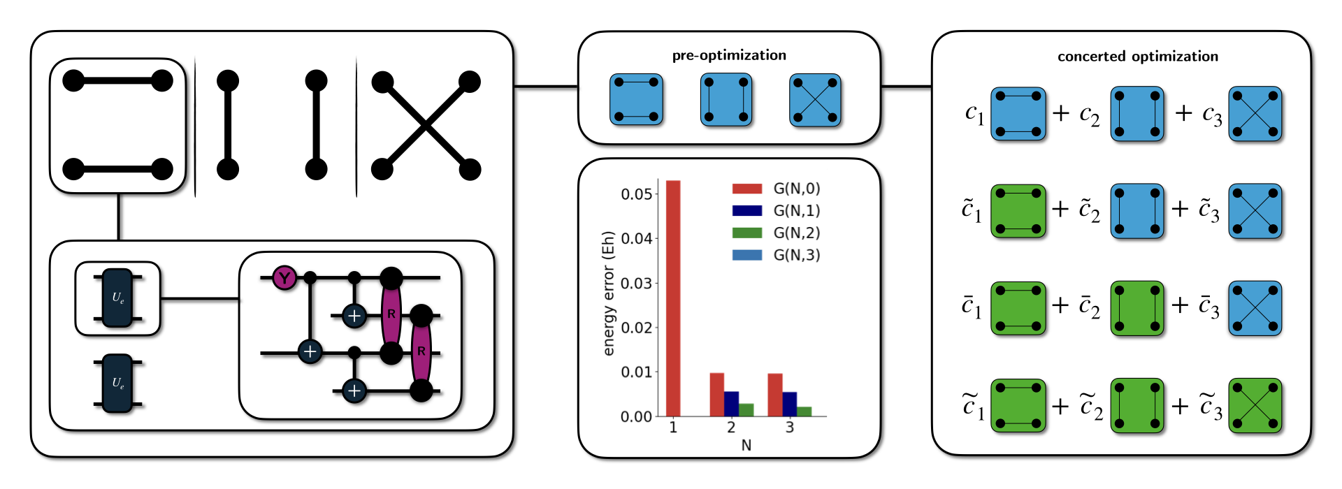
(a)

Figure 1: Basis construction: Illustration for the construction of many-body basis states through graph-based heuristics following [22]. On the left: the graphs with one of the corresponding SPA [31, 22] circuits of the quadratic H₄/STO-6G(4,8) constructed via Heuristic 1 in [22]. On the lower center: Energetic errors with different levels of optimization. $G(N,M\leq N)$ denotes the optimization (7) of parameters from $M$ circuits in a total wavefunction assembled from $N$ circuits as in Eq. (6). Note that the $G(3,3)$ error is essentially zero [32] and therefore not visible. On the right: illustration of the $G(N,M)$ wavefunctions obtained through concerted optimizations of the coefficients and angles from $M$ circuits with the corresponding graphs highlighted in green. From top to bottom the illustrations correspond to $G(3,0),G(3,1),G(3,2),G(3,3)$.

I Method

We start by selecting a suitable many-body basis in the form of parametrized quantum circuits

$$\ket{\psi\left(\boldsymbol{\theta}_{k}\right)}=U_{k}\left(\boldsymbol{\theta}_{k}\right)\ket{0},$$ (5)

in order to represent the total wavefunction

$$\ket{\Psi\left(\mathbf{c},\boldsymbol{\theta}\right)}=\sum_{k=1}^{N}c_{k}U_{k}\left(\boldsymbol{\theta}_{k}\right)\ket{0}.$$ (6)

Depending on the ground state problem of interest, the choice of the circuits $U_{k}$ will have practical implications on the runtime of the involved optimizations and the quality of the final wavefunction. In Sec. II we will discuss a specific choice of basis suitable for electronic structure, which we apply in this work.

Once the basis elements are chosen, a concerted optimization of all parameters in the total wavefunction (6) is performed

$$\left\{\mathbf{c}^{(*)},\boldsymbol{\theta}^{(*)}\right\}=\min_{\boldsymbol{c},\boldsymbol{{\theta}}^{(M)}}\frac{\langle\Psi\left(\mathbf{c},\boldsymbol{\theta}\right)\rvert H\lvert\Psi\left(\mathbf{c},\boldsymbol{\theta}\right)\rangle}{\langle\Psi\left(\mathbf{c},\boldsymbol{\theta}\right)|\Psi\left(\mathbf{c},\boldsymbol{\theta}\right)\rangle},$$ (7)

with $\boldsymbol{{\theta}}^{(M)}=\bigcup_{k=1}^{M}\left\{\boldsymbol{\theta}_{k}\right\}$ denoting the set of parameters subjected to the optimization procedure. Depending on the wavefunction and parameters in the optimization we use the notation $G(N,M)$ with $N$ denoting the number of circuits included in Eq. (6) and $M\leq N$ the number of fully optimized parameters $\boldsymbol{{\theta}}^{(M)}$. After the concerted optimization the generalized eigenvalue equation Eq. (1) is invoked as a convergence test. If the so-determined coefficients $\boldsymbol{c}$ differ from the optimized coefficients ${\boldsymbol{c}^{(*)}}$, the concerted optimization is restarted with the coefficients determined through (1) as starting values. This scheme proved to be useful in similar optimization frameworks in electronic structure. [33]

Prior to the optimization in Eq. (7), the circuit parameters can be initialized in the spirit of NOVQE [10] through individual energy optimization as in Eq. (3). At this point, it is crucial to avoid linear dependencies (i.e. restricting the overlaps $S_{ij}$ from becoming too close to one). [34] This can either be done by including penalty terms into the optimization or through the design of the individual circuits – in this work we resort to the latter (see Sec. II) and provide an argument (Sec. III) why this can be advantageous. The pre-optimized circuits are then subjected to the generalized eigenvalue equation (1) resulting in initial values for the coefficients $\mathbf{c}^{\text{(0)}}$ and initial energies which we will denote as $G(N,0)$.

II Circuits

In this work we will employ the circuit design principles of Ref. [22] in the context of fermionic Hamiltonians (encoded via Jordan-Wigner) in the usual form

$$H_{\text{f}}=\sum_{kl}h^{l}_{k}a^{\dagger}_{k}a_{l}+\sum_{klmn}g^{mn}_{kl}a^{\dagger}_{k}a^{\dagger}_{l}a_{m}a_{n},$$ (8)

with fermionic annihilation ($a_{k}$) and creation operators ($a^{\dagger}_{k}$) for electrons in the fermionic basis state (also called spin-orbital) $\chi_{k}(\mathbf{x})=\phi(\mathbf{x})\otimes\ket{\sigma_{k}}$ describing an electron with spin $\sigma_{k}\in\left\{\uparrow,\downarrow\right\}$ in the spatial orbital $\phi$. In the molecular case, the tensors $h$ and $g$ are computed as integrals over the states $\chi_{k}$ (for details see Ref. [8] or the appendix A of Ref. [22]). In this section we will resort to a short illustrative summary of the applied circuit designs.

Assume that we have a fermionic Hamiltonian as in Eq. (8) with $s$ spatial orbitals, and a collection of graphs $G(V,E)$, with vertices $V$ corresponding to sets of uniquely assigned orbitals and a set of non-overlapping edges. We can then construct a quantum circuit from that graph as

$$U_{\text{G}}=\bigotimes_{e\in E}U_{e}(\theta_{e})$$ (9)

where the individual circuits $U_{e}$ prepare a two-electron wavefunction on the qubits corresponding to the edge. The total wavefunction is then a $2|E|$-electron wavefunction and corresponds to a separable pair approximation [31] (see Heuristic 1 in [22] for more details). The circuits $U_{e}$ for the simplest non-trivial case: one orbital assigned to each vertex (corresponding to two spin-orbitals or qubits) are illustrated in Fig. 1 and consist of two parts

$$U_{e}=U\left(\theta\right)U_{\text{R}}\left(\varphi\right).$$ (10)

The first term $U(\theta)$ is built from a parametrized $R_{y}$ rotation and three controlled-NOT operations preparing the 4-qubit wavefunction

$$U\left(\theta\right)\ket{0}= \cos\left(\frac{\theta}{2}\right)\ket{1100}+\sin\left(\frac{\theta}{2}\right)\ket{0011}$$

$$\equiv \cos\left(\frac{\theta}{2}\right)\ket{\raisebox{-7.11317pt}{\includegraphics[width=17.34189pt]{configuration.001.png}}}+\sin\left(\frac{\theta}{2}\right)\ket{\raisebox{-7.11317pt}{\includegraphics[width=17.34189pt]{configuration.001x.png}}}.$$ (11)

Here, we used a graphical notation illustrating the two electrons in one of the two spatial basis states of the left and right vertex that form the edge $e$. As illustrated, $U(\theta)$ is moving a quasi-particle (often referred to as hard-core Boson) of two spin-paired electrons through the spatial basis states. However, the latter are not unique and we can transform the spatial part of the basis via linear combinations of the basis states. The second part of the circuit $U_{R}(\varphi)$ implements a unitary operation that corresponds to such a basis change (see Ref. [22] appendix B for details). Graphically this can be illustrated as

$$U_{\text{R}}\left(\varphi\right)\ket{\raisebox{-7.11317pt}{\includegraphics[width=17.34189pt]{configuration.001.png}}}\equiv \ket{\raisebox{-7.11317pt}{\includegraphics[width=17.34189pt]{configuration.002.png}}}$$ (12)

where the colors indicate positive and negative interference in the linear combination of the two basis states. In particular, the right hand side of Eq. (12) re-expresses the transformed wavefunction in the spatial orbitals $\tilde{\phi}_{1}=\cos(\varphi/2)\phi_{1}+\sin(\varphi)\phi_{2}$ and $\tilde{\phi}_{2}=\cos(\varphi/2)\phi_{1}-\sin(\varphi/2)\phi_{2}$.

Note that, in contrast to other works [31, 35, 36, 37] we are not restricting the total Hamiltonian to the hard-core Boson approximation, but rather express the total wavefunction as a linear combination of hard-core Bosonic wavefunctions in different orbital bases.

III Results

In the following we are applying the developed method to standard molecular benchmark systems used in Refs. [11, 10, 22] where we are interested mainly in the sizes of the effective bases sufficient to describe the electronic ground states. Through the circuit design described in the previous section, we are able to gain insights into the nature of the ground states.

The presented data is generated with tequila [38, 9], where we give explicit code examples in the appendix B. In the computational process, the following dependencies were utilized in the background: qulacs [39] as quantum backend, BFGS implementation within scipy [40] as optimizer, pyscf [41, 42] to compute molecular integrals (forming the tensors of the Hamiltonian in Eq. (8)) and exact energies, and the Jordan-Wigner encoding from openfermion [43]. The MRSQK energies were computed with qforte [44].

III.1 The H₄ Square System: insights from an explicit example

In Fig. 1 the $G(N,M<N)$ method is illustrated on the H₄/STO-3G(4,8) square system consisting of four hydrogen atoms, each equipped with a single orbital from the STO-6G set, equidistantly placed on a rectangle with vertex distances set close to the equilibrium distance of a single H₂ molecule ($d=1.5\AA$). Following  22 we can construct three possible molecular graphs and the corresponding circuits illustrated in Fig. 1 representing the total wavefunction in Eq. (6) with parameters optimized according to Eq. (7). From Fig.1 we see that a concerted optimization over all three graphs $G(3,3)$ yields the exact energy. There is however no visible difference between $G(2,M)$ and $G(3,M)$ with $M\neq 3$ meaning that inclusion of the third graph only has an effect in a concerted optimization.

The wavefunction prepared by the circuit derived from the third graph state optimized on G(3,3) level - i.e. in a concerted optimization including all three graphs - takes the form

$$\ket{\raisebox{-7.11317pt}{\includegraphics[width=17.34189pt]{graph-crossed-green.png}}}=\frac{1}{2}\left(\ket{\raisebox{-7.11317pt}{\includegraphics[width=17.34189pt]{configuration.008.png}}}+\ket{\raisebox{-7.11317pt}{\includegraphics[width=17.34189pt]{configuration.009.png}}}-\ket{\raisebox{-7.11317pt}{\includegraphics[width=17.34189pt]{configuration.010.png}}}-\ket{\raisebox{-7.11317pt}{\includegraphics[width=17.34189pt]{configuration.011.png}}}\right),$$ (13)

Here the up (and down) arrows represent a spin-up (spin-down) electron occupying one of the four spatial orbitals located on the hydrogen atoms. The state in Eq.(13) is assembled from four configurations that cluster the four electrons as close as possible. The wavefunction clearly is energetically not favorable explaining the failure of energy based pre-optimization in the $G(3,M<3)$ wavefunctions. The reason why the state in Eq.(13) needs to take this specific form becomes clear when we take a look at the $G(2,2)$ wavefunction

$$\ket{G(2,2)}= \bar{c}_{1}\ket{\raisebox{-7.11317pt}{\includegraphics[width=17.34189pt]{graph-green.png}}}+\bar{c}_{2}\ket{\raisebox{-7.11317pt}{\includegraphics[width=17.34189pt]{graph2-green.png}}}$$

$$= a\left(\ket{\raisebox{-7.11317pt}{\includegraphics[width=17.34189pt]{configuration.008.png}}}+\ket{\raisebox{-7.11317pt}{\includegraphics[width=17.34189pt]{configuration.009.png}}}-\ket{\raisebox{-7.11317pt}{\includegraphics[width=17.34189pt]{configuration.010.png}}}-\ket{\raisebox{-7.11317pt}{\includegraphics[width=17.34189pt]{configuration.011.png}}}\right)$$

$$+b\ket{\Psi_{\text{R}}}$$

$$= 2a\ket{\raisebox{-8.5359pt}{\includegraphics[width=19.5121pt]{graph-crossed-green.png}}}+b\ket{\Psi_{\text{R}}}$$ (14)

with the amplitudes $\bar{c}_{2}=-\bar{c}_{1}$ and $a\approx 0.07<b$ and $\Psi_{\text{R}}$ contains all other electronic configurations. We see from Eq. (III.1) that the (optimized) wavefunction of the third graph (13) is already included. Adding the third graph to the total wavefunction in $G(3,3)$ does therefore not introduce new configurations into the total wavefunction but it allows a relative reduction of the amplitude $a$ while preserving the internal structure of the residual (and energetically more important) wavefunction $\ket{\Psi_{\text{R}}}$ – the structure of the $G(2,2)$ wavefunction alone would not allow this. On the other hand, energy based pre-optimization of the third graph does not result in the energetically unfavorable form of Eq. (13) leading to $G(3,2)$ having no visible improvement over $G(2,2)$ as witnessed in Fig. 1. The analysis of the wavefunctions in Eq. (13) and (III.1) also shows why orthogonality constraints between the individual graphs in the optimization can become problematic.

When compared to two isolated H₂ molecules the optimal wavefunction of the third graph would correspond to a product of two ionic non-bonding states, as it can be written as

$$\ket{\raisebox{-7.11317pt}{\includegraphics[width=17.34189pt]{graph-crossed-green.png}}}=\frac{1}{2}\left(\ket{\raisebox{-7.11317pt}{\includegraphics[width=17.34189pt]{configuration.004.png}}}-\ket{\raisebox{-7.11317pt}{\includegraphics[width=17.34189pt]{configuration.006.png}}}\right)\otimes\left(\ket{\raisebox{-7.11317pt}{\includegraphics[width=17.34189pt]{configuration.005.png}}}-\ket{\raisebox{-7.11317pt}{\includegraphics[width=17.34189pt]{configuration.007.png}}}\right)$$ (15)

while the corresponding wavefunctions of the other two graphs have more similarity with a product of bonding H₂ wavefunctions. The intuitive picture of the $G(2,2)$ wavefunction in Eq. (III.1) that represents the H₄ wavefunction as a superposition of both degenerate realizations of two individual H₂ molecules is therefore still a reasonable model for the true ground state of the system. A suitable interpretation for the third graph is the addition of weak correlation between the two isolated H₂ molecules achieved by destructive interference of energetically unfavorable configurations. This allows an interesting connection to Ref. [23] (in particular Fig. 4) where similar effects were identified in the context of quantum optical setups and similar arguments as in this case will hold for potential future approaches based on individual optimization.

A further illustration of the weak type of correlation contributed by the third graph, is to take a wavefunction generated by the first two graphs, but with more flexibility in the individual circuits. In this case we added more orbital rotations to the circuit (denoted by $U_{\text{R}}$ in the corresponding methods), so that all non-connected vertices of the graphs were connected through an orbital rotation. With this, the $G(2,2)+U_{\text{R}}$ wavefunction is sufficient to represent the true ground state with arbitrary precision [32].

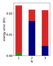
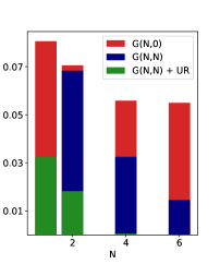
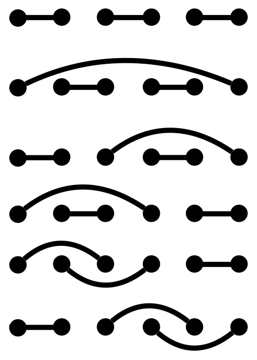
(a) H₄, $r=1.5$Å     (b) H₆, $r=1.5$Å     (c)

Figure 2: Effects of optimization level and circuit expressivity on linear hydrogen chains (equidistant bond lengths of 1.5Å). Basic circuits are constructed analogously to Fig. 1. For $G(N,)+UR$ datapoints the circuits were augmented with additional orbital rotations. (a): H₄/STO-6G(4,8) (b): H₆/STO-6G(6,12), (c): graphs used for H₆/STO-6G(6,12).

Method	H4	H6
MRSQK (m=1)	2656	19944
MRSQK (m=8)	21248	159552
UpCCGSD	188	687
2-UpCCGSD	432	1387
$G(N,M)$	70	150
$G(N,M)+U_{\text{R}}$	150	425

Table 1: CNOT counts of the deepest circuit in MRSQK [45], NO-VQE with $k$-UpCCGSD (compiled with optimizations introduced in [31]) and the $G(M,N)$ developed in this work. Note further reduction could be achieved through more efficient compiling of the $U_{\text{R}}$ rotations  [46, 47]

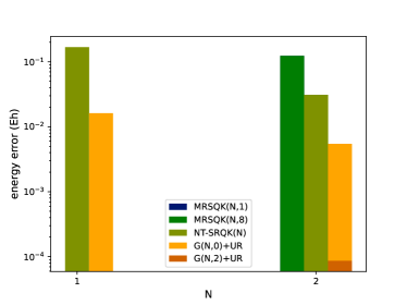
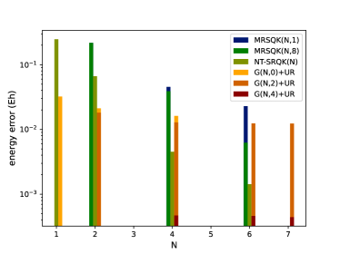
(a) H₄, $r=1.5$Å (b) H₆, $r=1.5$Å

Figure 3: Comparison of the present approach with the multireference selected quantum krylov approach (MRSQK) [11] with respect to the number $N$ of used effective many-body basis states. Energy errors w.r.t. the exact ground state are given for (a) H₄/STO-6G(4,8) and (b) H₆/STO-6G(6,12). MRSQK($N,m$) and NT-SRQK($N$) results are with, and without, Trotter approximation using $m$ Trotter steps for the real-time evolution. Graph based construction is done according to Fig. 1 with static energies denoting the ground state of the effective Hamiltonian in the pre-optimized basis. $G(N,M)$ denotes energies of wavefunctions according to Eq. (7) using $N$ graphs to construct $N$ circuits $U_{k}$ with $M$ of them being fully optimized in a concerted optimization. Note that in the H₄ case using 1 or 8 Trotter steps leads to the same error.

III.2 Linear H₄ and H₆: comparison to quantum Krylov

In the previous Section, we have seen how the individual parts of the wavefunction can be interpreted. We have identified weak correlations (as in the third graph of the rectangular H₄) that can not be generated through energy based pre-optimization as the energetic effect is due to destructive interference and only present in the total wavefunction. In the case of the rectangular H₄ those weak correlations could be compensated by equipping the circuits representing the individual graphs with more freedom in the form of orbital rotations. We expect a similar behavior for other systems and tested it on the linear H₄ and H₆ models where the results displayed in Fig. 2 show the same trends as observed before. While the non augmented wavefunctions show good convergence within the first 3, respectively 6, graphs, the overall error is still around 5, respectively 10, millihartree for the fully optimized wavefunctions. On the other hand, the augmented $G(N,M=N)+U_{\text{R}}$ wavefunction already achieves chemical accuracy at a smaller size $N$ of the effective many-body basis.

The linear H₄ and H₆ hydrogen chains are prominent benchmark systems that have been applied in the context of Refs. [22] as well as in Ref. [11] that introduced the Multi-Reference Selected Quantum Krylov (MRSQK) method – a real-time evolution approach towards approximating the Krylov subspace in Eq. (4). In Fig. 3 we compare the $G(N,M)+U_{\text{R}}$ energies with MRSQK with respect to the size of the many-body basis $N$ that is for our method the number of graph-based circuits and for MRSQK the number of multi-reference starting points of the real-time evolution. We see that $G(N,N)$ always outperforms MRSQK in all flavors while $G(N>2,2)$ energies can not improve upon the non-Trotterized quantum Krylov variant and $G(N>4,0)$ can not improve upon the Trotterized variant with 8 Trotter steps. Based on the observations on the rectangular H₄ example, this is not further surprising as we would expect the higher order graphs only to bring significant improvements when they are included into the concerted optimization. Note that apart from the basis size $N$ the $G(N,M)$ method requires significantly shallower circuits compared to the Trotterized real-time evolutions necessary to generate the MRSQK basis (see Tab. 1). In comparison to NO-VQE [10] the circuit sizes are still significantly reduced and the method in this work is not relying on repeated randomized initialization. The total number of BFGS iterations is moderate (varying between 15 and 30 iterations) and we expect further reduction through improved implementations.

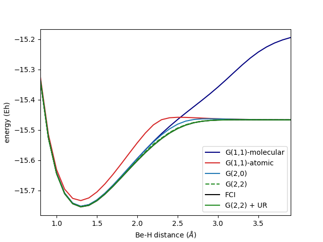
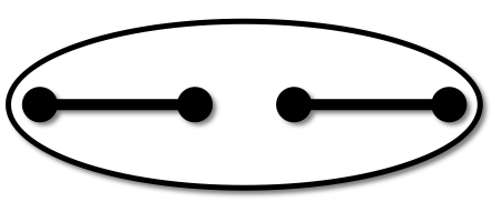
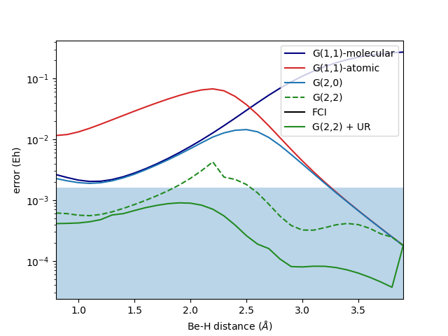
(a) (b)

Figure 4: BeH₂/STO-6G(4,8) energies from $G(N,M\leq N)$ wavefunctions constructed analog to Fig. 1. (a): absolute energies with dominant molecular graphs shown as insets, (b): energies relative to FCI/STO-6G(4,8) with the 1 kcal/mol accuracy region highlighted in blue. $G(2,2)+U_{R}$ denotes the same procedure with additional orbital rotators in the individual circuits.

III.3 Linear BeH₂: transferring concepts from H₄ to a more complex system

In Ref. [22] the graph based construction was applied for a single circuit to prepare the wavefunction directly, while in this work we resorted to a divided approach where each graph corresponds to an individual circuit. In the previous section we have seen, that the divided approach here can achieve comparable accuracy in the wavefunctions. So far, we resorted to simplified hydrogenic systems with a single spherical s-type orbital on each atom. With BeH₂/STO-6G(4,8) we add a model system with more complicated orbital structure (having s- and p-type orbitals on the central Be atom). This model system is the same as in [22] and has the same dimensions as H₄/STO-6G(4,8). Through the graph description we can treat the BeH₂ now in the same way as the linear H₄. The two main graphs are illustrated in Fig. 4, where one of them is interpreted as molecular and the other as atomic (see also Eq. (25) in [22]). In Fig. 4 we clearly see how the potential energy surface is divided into three domains: the first being the bonded domain (around bond distance $R=1.5$Å), the second the dissociated domain ($R>3.0$Å) both dominated by a single graph, while the third domain (around $R=2.6$Å) requires both graphs for an accurate description.

IV Conclusion & Outlook

Since the advent of variational quantum eigensolver [4, 3] efficient ways to prepare fermionic ground states were investigated through different routes [5, 6]. Despite having a vast set of methods it is still not clear which method performs well for which systems. In this work we provided a first step into that direction by combining interpretable circuit designs with a divide-and-conquer approach where the wavefunction is assembled as a linear combination of smaller parts. We could show, how this method outperforms other divide-and-conquer methods in terms of size of the effective basis as well as individual quantum resources for the involved circuits. Most importantly the developed method allows us to interpret the results and to learn from the discovered effects.
At this point, the computational bottleneck comes with the concerted optimization necessary for the determination of the effective basis. As a quantum algorithm, this procedure requires many evaluation of primitive expectation values (in the sense of [38]). We see however promising ways forward in that respect, as illustrated in the following. Through the combination with the circuit designs of [22] the effective basis is described by individual circuits that are equivalent to separable pair approximations [31]. As a consequence, the individual wavefunctions are classically simulable, so that energy based pre-optimization can be performed purely classical with linear memory requirement. The $G(N,0)$ method therefore defines a de-quantized and de-randomized flavor of a NO-VQE. Based on the reported numerical evidence, we expect this to work well for qualitative descriptions of the wavefunctions. For a quantitative treatment, energy based pre-optimization is however not expected to be practicable. Other types of pre-optimizations, as in Ref. [48], could however be imagined for the future and might lead to more powerful purely classical methods capable of generating compact quantum circuits for accurate state preparation. The interpretable circuit design offers here a chance to effectively predict optimal circuit parameters based on detailed analysis of model systems.

V Acknowledgment

This project was initiated through the Mentorship Program of the Quantum Open Source Foundation (QOSF) Cohort 5. [49] We are grateful to the QOSF for providing this platform. We thank Philipp Schleich for giving valuable feedback to the initial manuscript. Furthermore we thank Nick Stair and Francesco Evangelista for providing user-friendly public access to the MRSQK [11] method through qforte [44].

Appendix A Explicit qubit states for the graphical depictions in the main text

In the main text we resorted to graphical symbols to represent electronic configurations in the rectangular H₄ system. Here we show the corresponding configurations as qubit states in Jordan-Wigner encoding - meaning they are identical to standard occupation number vectors in second quantized formulation. The qubit represent spin orbitals (even qubits spin-up and odd qubits spin-down) and the orbitals are orthonormalized atomic basis orbitals of the STO-3G set - meaning one spherical symmetrical s-type orbital for each of the four H atoms in clockwise order. The four configurations featuring four electrons are

$$\ket{\raisebox{-8.5359pt}{\includegraphics[width=19.5121pt]{configuration.008.png}}}= \ket{11000011}, \ket{\raisebox{-8.5359pt}{\includegraphics[width=19.5121pt]{configuration.009.png}}}= \ket{11110000},$$ (16)

$$\ket{\raisebox{-8.5359pt}{\includegraphics[width=19.5121pt]{configuration.010.png}}}= \ket{00001111}, \ket{\raisebox{-8.5359pt}{\includegraphics[width=19.5121pt]{configuration.011.png}}}= \ket{00110011}.$$ (17)

The two electron states represent the configuration on a reduced orbital set given by the edge of the graph

$$\ket{\raisebox{-8.5359pt}{\includegraphics[width=19.5121pt]{configuration.004.png}}}= \ket{1100}_{0145}, \ket{\raisebox{-8.5359pt}{\includegraphics[width=19.5121pt]{configuration.005.png}}}= \ket{0011}_{2367},$$ (18)

$$\ket{\raisebox{-8.5359pt}{\includegraphics[width=19.5121pt]{configuration.006.png}}}= \ket{0011}_{0145}, \ket{\raisebox{-8.5359pt}{\includegraphics[width=19.5121pt]{configuration.007.png}}}= \ket{1100}_{2367},$$ (19)

Here, the subscripts denote the qubit indices in order for the result of the tensor products in the main text to be in the right order. This is meant in the following way:

$$\ket{\raisebox{-8.5359pt}{\includegraphics[width=19.5121pt]{configuration.004.png}}}\otimes\ket{\raisebox{-8.5359pt}{\includegraphics[width=19.5121pt]{configuration.005.png}}}= \ket{1100}_{0145}\otimes\ket{0011}_{2367}=\ket{11000011}=\ket{\raisebox{-8.5359pt}{\includegraphics[width=19.5121pt]{configuration.008.png}}}$$ (21)

Appendix B Explicit code example

In Figs. 5 and 6 explicit code examples to reproduce the data in Fig. 1 is provided. The code can be viewed as pseudocode, it is however executable with tequila [38] (version 1.8.4) and numpy [50](version 1.21.5). The code requires psi4 [51] or pyscf [41, 42] to be installed (in order to compute the molecular integrals) and it is recommended to have qulacs [39] installed as wavefunction simulation backend. In the first block, the $G(N,M)$ function is defined. Note that we used a different implementation that exploits some shortcuts in the classical simulation - this is provided on an external github repository [52].

⬇

1# tq.version.__version__ >= 1.8.5

2import tequila as tq

3import numpy

4

5def G(N,M,H,U,initial_values):

6 print(N," ",M)

7 assert M <= N

8 assert N <= len(U)

9

10 # initial values for coefficients through GEM (Eq.1)

11 v,vv = tq.apps.gem(U, H, variables=initial_values)

12

13 # initialize variables for coefficients

14 c = [tq.Variable(("c",i)) for i in range(N)]

15

16 for i in range(N):

17 initial_values[c[i]]=vv[i,0]

18

19 # Initialize the objective of Eq.7

20 # by expanding with wavefunction of Eq.6

21 ED = 0.0

22 EN = 0.0

23 for i in range(N):

24 for j in range(N):

25 # only need real part of braket (by construction)

26 EN += c[i]*c[j]*tq.braket(U[i],U[j],H)[0]

27 ED += c[i]*c[j]*tq.braket(U[i],U[j])[0]

28

29 E = EN/ED

30

31 # active variables for the concerted optimization

32 active = sum([U[i].extract_variables() for i in range(M)],[])

33 active += c

34

35 # gradient compilation not optimized for tq.braket

36 # recommending to use finite-differences

37 result = tq.minimize(E, variables=active, initial_values=initial_values, gradient="2-point", method_options={"finite_diff_rel_step":1.e-4})

38

39 return result

Figure 5: Implementation of the $G(N,M)$ method introduced in the main text

⬇

1# define the molecule

2geometry = "H 1.5 0.0 0.0\nH 0.0 0.0 0.0\nH 1.5 0.0 1.5\nH 0.0 0.0 1.5"

3mol = tq.Molecule(geometry=geometry, basis_set="sto-6g")

4# use orthonormalized atomic orbitals

5mol = mol.use_native_orbitals()

6

7# Define the qubit Hamiltonian

8H = mol.make_hamiltonian()

9# get the reference energy

10exact = mol.compute_energy("fci")

11

12# define the graphs

13G1 = [(0,1),(2,3)]

14G2 = [(0,2),(1,3)]

15G3 = [(0,3),(1,2)]

16graphs = [G1, G2, G3]

17

18# define the circuits to generate the basis

19circuits = []

20for i,edges in enumerate(graphs):

21 # label to prevent identical variable names in different circuits

22 label="G{}".format(i+1)

23 U = mol.make_ansatz(name="SPA", edges=edges, label=label)

24 for e in edges:

25 U += mol.UR(e[0],e[1],label=label)

26 circuits.append(U)

27

28# pre-optimize the circuits

29variables = {}

30for U in circuits:

31 E = tq.ExpectationValue(U=U, H=H)

32 result = tq.minimize(E, silent=True)

33 variables = {**variables, **result.variables}

34 print("Graph {}: with energy {:+2.5f}".format(i, result.energy))

35

36# run the G(N,M) computations

37energies={}

38for N in range(1,4):

39 for M in range(1,N):

40 result = G(N,M,H,circuits,variables)

41 variables = result.variables

42 energies["G({},{})".format(N,M)]=result.energy

Figure 6: Compute the data shown in Fig. 1 in the main text. Content of Fig. 5 needs to be imported.

Appendix C Details on related works

In the introduction of the main text, several methods that try to approximate the Krylov subspace in Eq. (4) where grouped together. These works take different routes to approximate the $\ket{\psi_{k}}\in\mathcal{K}$. In [12, 13, 14] Quantum Imaginary Time evolution (QITE) is employed while [11] resorts to real-time evolution on multiple initial states defining a Multi-Reference selected Quantum Krylov (MRSQK) approach. Similar to MRSQK are the quantum filter diagonalization (QFD) [15, 16] and the variational assisted quantum simulator (QAS) [bharti2020qav, 17, 18]. The QFD relies on real-time simulation in the same spirit as MRSQK while QAS approximates powers of the Hamiltonian by creating products of individual unitaries (paulistrings) that define it. In a similar fashion, an inverse power method (using $H^{-k}$) has been proposed with analogue quantum simulators in mind. [19] Recently, direct unitary encoding of the Hamiltonian powers was proposed in [20] (via linear combination of unitaries) and [21] (via block-encoding).
Related to the non-orthogonal variational quantum eigensolvers (NOVQE [10]) are NOVQEs with classical preoptimized parameters (NOQE [48]), variational quantum subspace expansion [53, 54, 55, 56] and entirely classical approaches like NOMAGIC [57]. The NOQE method in particular introduces an interesting alternative for pre-screening of parameters.

References

- Bharti et al. [2022] K. Bharti, A. Cervera-Lierta, T. H. Kyaw, T. Haug, S. Alperin-Lea, A. Anand, M. Degroote, H. Heimonen, J. S. Kottmann, T. Menke, et al., Noisy intermediate-scale quantum algorithms, Reviews of Modern Physics 94, 015004 (2022).
- Cerezo et al. [2021] M. Cerezo, A. Arrasmith, R. Babbush, S. C. Benjamin, S. Endo, K. Fujii, J. R. McClean, K. Mitarai, X. Yuan, L. Cincio, et al., Variational quantum algorithms, Nature Reviews Physics 3, 625 (2021).
- McClean et al. [2016] J. R. McClean, J. Romero, R. Babbush, and A. Aspuru-Guzik, The theory of variational hybrid quantum-classical algorithms, New J. Phys. 18, 023023 (2016).
- Peruzzo et al. [2014] A. Peruzzo, J. McClean, P. Shadbolt, M.-H. Yung, X.-Q. Zhou, P. J. Love, A. Aspuru-Guzik, and J. L. O’brien, A variational eigenvalue solver on a photonic quantum processor, Nat. Commun. 5, 4213 (2014).
- Anand et al. [2022a] A. Anand, P. Schleich, S. Alperin-Lea, P. W. K. Jensen, S. Sim, M. Díaz-Tinoco, J. S. Kottmann, M. Degroote, A. F. Izmaylov, and A. Aspuru-Guzik, A quantum computing view on unitary coupled cluster theory, Chem. Soc. Rev. 51, 1659 (2022a).
- Tilly et al. [2020] J. Tilly, G. Jones, H. Chen, L. Wossnig, and E. Grant, Computation of molecular excited states on ibm quantum computers using a discriminative variational quantum eigensolver, Phys. Rev. A 102, 062425 (2020).
- Lee et al. [2018] J. Lee, W. J. Huggins, M. Head-Gordon, and K. B. Whaley, Generalized unitary coupled cluster wave functions for quantum computation, J. Chem. Theory Comput. 15, 311 (2018).
- Kottmann et al. [2021a] J. S. Kottmann, P. Schleich, T. Tamayo-Mendoza, and A. Aspuru-Guzik, Reducing qubit requirements while maintaining numerical precision for the variational quantum eigensolver: A basis-set-free approach, J. Phys. Chem. Lett. 12, 663 (2021a).
- Kottmann et al. [2021b] J. S. Kottmann, A. Anand, and A. Aspuru-Guzik, A feasible approach for automatically differentiable unitary coupled-cluster on quantum computers, Chemical science 12, 3497 (2021b).
- Huggins et al. [2020] W. J. Huggins, J. Lee, U. Baek, B. O’Gorman, and K. B. Whaley, A non-orthogonal variational quantum eigensolver, New Journal of Physics 22, 073009 (2020).
- Stair et al. [2020] N. H. Stair, R. Huang, and F. A. Evangelista, A multireference quantum krylov algorithm for strongly correlated electrons, J. Chem. Theory Comput. 16, 2236 (2020).
- Yeter-Aydeniz et al. [2019] K. Yeter-Aydeniz, R. C. Pooser, and G. Siopsis, Practical quantum computation of chemical and nuclear energy levels using quantum imaginary time evolution and lanczos algorithms 10.48550/arxiv.1912.06226 (2019).
- Motta et al. [2020] M. Motta, C. Sun, A. T. Tan, M. J. O’Rourke, E. Ye, A. J. Minnich, F. G. Brandão, and G. K.-L. Chan, Determining eigenstates and thermal states on a quantum computer using quantum imaginary time evolution, Nat. Phys. 16, 205 (2020).
- Tsuchimochi et al. [2022] T. Tsuchimochi, Y. Ryo, and S. L. Ten-no, Multi-state quantum simulations via model-space quantum imaginary time evolution 10.48550/arxiv.2206.04494 (2022).
- Parrish and McMahon [2019] R. M. Parrish and P. L. McMahon, Quantum filter diagonalization: Quantum eigendecomposition without full quantum phase estimation, arxiv:1909.08925 (2019).
- Cohn et al. [2021] J. Cohn, M. Motta, and R. M. Parrish, Quantum filter diagonalization with compressed double-factorized hamiltonians, PRX Quantum 2, 040352 (2021).
- Bharti and Haug [2021a] K. Bharti and T. Haug, Quantum-assisted simulator, Phys. Rev. A 104, 042418 (2021a).
- Bharti and Haug [2021b] K. Bharti and T. Haug, Iterative quantum-assisted eigensolver, Phys. Rev. A 104, L050401 (2021b).
- Kyriienko [2020] O. Kyriienko, Quantum inverse iteration algorithm for programmable quantum simulators, npj Quantum Inf. 6, 1 (2020).
- Seki and Yunoki [2021] K. Seki and S. Yunoki, Quantum power method by a superposition of time-evolved states, PRX Quantum 2, 010333 (2021).
- Kirby et al. [2022] W. Kirby, M. Motta, and A. Mezzacapo, Exact and efficient lanczos method on a quantum computer 10.48550/arxiv.2208.00567 (2022).
- Kottmann [2022] J. S. Kottmann, Molecular quantum circuit design: A graph-based approach 10.48550/arxiv.2207.12421 (2022).
- Krenn et al. [2021] M. Krenn, J. S. Kottmann, N. Tischler, and A. Aspuru-Guzik, Conceptual understanding through efficient automated design of quantum optical experiments, Phys. Rev. X 11, 031044 (2021).
- Kottmann et al. [2021c] J. S. Kottmann, M. Krenn, T. H. Kyaw, S. Alperin-Lea, and A. Aspuru-Guzik, Quantum computer-aided design of quantum optics hardware, Quantum Science and Technology 6, 035010 (2021c).
- Ruiz-Gonzalez et al. [2022] C. Ruiz-Gonzalez, S. Arlt, J. Petermann, S. Sayyad, T. Jaouni, E. Karimi, N. Tischler, X. Gu, and M. Krenn, Digital discovery of 100 diverse quantum experiments with pytheus 10.48550/arxiv.2210.09980 (2022).
- Arlt et al. [2022] S. Arlt, C. Ruiz-Gonzalez, and M. Krenn, Digital discovery of a scientific concept at the core of experimental quantum optics 10.48550/arxiv.2210.09981 (2022).
- Schuld et al. [2021] M. Schuld, R. Sweke, and J. J. Meyer, Effect of data encoding on the expressive power of variational quantum-machine-learning models, Physical Review A 103, 032430 (2021).
- Anand et al. [2022b] A. Anand, L. B. Kristensen, F. Frohnert, S. Sim, and A. Aspuru-Guzik, Information flow in parameterized quantum circuits 10.48550/arxiv.2207.05149 (2022b).
- Heese et al. [2023] R. Heese, T. Gerlach, S. Mücke, S. Müller, M. Jakobs, and N. Piatkowski, Explainable quantum machine learning 10.48550/arxiv.2301.09138 (2023).
- Casas and Cervera-Lierta [2023] B. Casas and A. Cervera-Lierta, Multi-dimensional fourier series with quantum circuits, arXiv preprint arXiv:2302.03389 https://doi.org/10.48550/arXiv.2302.03389 (2023).
- Kottmann and Aspuru-Guzik [2022] J. S. Kottmann and A. Aspuru-Guzik, Optimized low-depth quantum circuits for molecular electronic structure using a separable-pair approximation, Phys. Rev. A 105, 032449 (2022).
- not [Fig1] (Concerns Fig.1), the energy error of for the rectangular H4 are close to the ground state are around with the scipy BFGS optimizer (default settings).
- Kottmann et al. [2015] J. S. Kottmann, S. Höfener, and F. A. Bischoff, Numerically accurate linear response-properties in the configuration-interaction singles (cis) approximation, Phys. Chem. Chem. Phys. 17, 31453 (2015).
- Epperly et al. [2022] E. N. Epperly, L. Lin, and Y. Nakatsukasa, A theory of quantum subspace diagonalization, SIAM Journal on Matrix Analysis and Applications 43, 1263 (2022).
- Elfving et al. [2021] V. E. Elfving, M. Millaruelo, J. A. Gámez, and C. Gogolin, Simulating quantum chemistry in the seniority-zero space on qubit-based quantum computers, Phys. Rev. A 103, 032605 (2021).
- Khamoshi et al. [2022] A. Khamoshi, G. P. Chen, F. A. Evangelista, and G. E. Scuseria, Agp-based unitary coupled cluster theory for quantum computers (2022).
- Zhao et al. [2022] L. Zhao, J. Goings, K. Wright, J. Nguyen, J. Kim, S. Johri, K. Shin, W. Kyoung, J. I. Fuks, J.-K. K. Rhee, and Y. M. Rhee, Orbital-optimized pair-correlated electron simulations on trapped-ion quantum computers 10.48550/arxiv.2212.02482 (2022).
- Kottmann et al. [2021d] J. S. Kottmann, S. Alperin-Lea, T. Tamayo-Mendoza, A. Cervera-Lierta, C. Lavigne, T.-C. Yen, V. Verteletskyi, P. Schleich, A. Anand, M. Degroote, S. Chaney, M. Kesibi, N. G. Curnow, B. Solo, G. Tsilimigkounakis, C. Zendejas-Morales, A. F. Izmaylov, and A. Aspuru-Guzik, TEQUILA: a platform for rapid development of quantum algorithms, Quantum Science and Technology 6, 024009 (2021d).
- Suzuki et al. [2021] Y. Suzuki, Y. Kawase, Y. Masumura, Y. Hiraga, M. Nakadai, J. Chen, K. M. Nakanishi, K. Mitarai, R. Imai, S. Tamiya, T. Yamamoto, T. Yan, T. Kawakubo, Y. O. Nakagawa, Y. Ibe, Y. Zhang, H. Yamashita, H. Yoshimura, A. Hayashi, and K. Fujii, Qulacs: a fast and versatile quantum circuit simulator for research purpose, Quantum 5, 559 (2021).
- Virtanen et al. [2020] P. Virtanen, R. Gommers, T. E. Oliphant, M. Haberland, T. Reddy, D. Cournapeau, E. Burovski, P. Peterson, W. Weckesser, J. Bright, S. J. van der Walt, M. Brett, J. Wilson, K. Jarrod Millman, N. Mayorov, A. R. J. Nelson, E. Jones, R. Kern, E. Larson, C. Carey, İ. Polat, Y. Feng, E. W. Moore, J. Vand erPlas, D. Laxalde, J. Perktold, R. Cimrman, I. Henriksen, E. A. Quintero, C. R. Harris, A. M. Archibald, A. H. Ribeiro, F. Pedregosa, P. van Mulbregt, and S. . . Contributors, SciPy 1.0: Fundamental Algorithms for Scientific Computing in Python, Nature Methods 17, 261 (2020).
- Sun et al. [2018] Q. Sun, T. C. Berkelbach, N. S. Blunt, G. H. Booth, S. Guo, Z. Li, J. Liu, J. D. McClain, E. R. Sayfutyarova, S. Sharma, S. Wouters, and G. K.-L. Chan, Pyscf: the python-based simulations of chemistry framework, Wiley Interdiscip. Rev. Comput. Mol. Sci. 8, e1340 (2018).
- Sun et al. [2020] Q. Sun, X. Zhang, S. Banerjee, P. Bao, M. Barbry, N. S. Blunt, N. A. Bogdanov, G. H. Booth, J. Chen, Z.-H. Cui, J. J. Eriksen, and et. al., Recent developments in the pyscf program package, J. Chem. Phys. 153, 024109 (2020).
- McClean et al. [2020a] J. McClean, N. Rubin, K. Sung, I. D. Kivlichan, X. Bonet-Monroig, Y. Cao, C. Dai, E. S. Fried, C. Gidney, B. Gimby, et al., Openfermion: the electronic structure package for quantum computers, Quantum Sci. Technol. (2020a).
- Stair and Evangelista [2022] N. H. Stair and F. A. Evangelista, Qforte: An efficient state-vector emulator and quantum algorithms library for molecular electronic structure, Journal of Chemical Theory and Computation 18, 1555 (2022).
- not [unts] (Note on MRSQK CNOT counts), data taken from qforte output. We expect this to be further reducible with advanced compilation techniques.
- Kivlichan et al. [2018] I. D. Kivlichan, J. McClean, N. Wiebe, C. Gidney, A. Aspuru-Guzik, G. K.-L. Chan, and R. Babbush, Quantum simulation of electronic structure with linear depth and connectivity, Phys. Rev. Lett. 120, 110501 (2018).
- Quantum et al. [2020] G. A. Quantum, Collaborators*†, F. Arute, K. Arya, R. Babbush, D. Bacon, J. C. Bardin, R. Barends, S. Boixo, M. Broughton, B. B. Buckley, et al., Hartree-fock on a superconducting qubit quantum computer, Science 369, 1084 (2020).
- Baek et al. [2022] U. Baek, D. Hait, J. Shee, O. Leimkuhler, W. J. Huggins, T. F. Stetina, M. Head-Gordon, and K. B. Whaley, Say no to optimization: A non-orthogonal quantum eigensolver 10.48550/arxiv.2205.09039 (2022).
- QOSF [2020] QOSF, Quantum open source foundation, https://qosf.org/ (2020).
- Harris et al. [2020] C. R. Harris, K. J. Millman, S. J. van der Walt, R. Gommers, P. Virtanen, D. Cournapeau, E. Wieser, J. Taylor, S. Berg, N. J. Smith, R. Kern, M. Picus, S. Hoyer, M. H. van Kerkwijk, M. Brett, A. Haldane, J. F. del Río, M. Wiebe, P. Peterson, P. Gérard-Marchant, K. Sheppard, T. Reddy, W. Weckesser, H. Abbasi, C. Gohlke, and T. E. Oliphant, Array programming with NumPy, Nature 585, 357 (2020).
- Smith et al. [2020] D. G. Smith, L. A. Burns, A. C. Simmonett, R. M. Parrish, M. C. Schieber, R. Galvelis, P. Kraus, H. Kruse, R. Di Remigio, A. Alenaizan, et al., Psi4 1.4: Open-source software for high-throughput quantum chemistry, J. Chem. Phys. 152, 184108 (2020).
- git [tory] special implementations of the techniques in this work are provided here: github.com/kottmanj/compact-bases (online repository).
- McClean et al. [2020b] J. R. McClean, Z. Jiang, N. C. Rubin, R. Babbush, and H. Neven, Decoding quantum errors with subspace expansions, Nat. Commun. 11, 636 (2020b).
- Takeshita et al. [2020] T. Takeshita, N. C. Rubin, Z. Jiang, E. Lee, R. Babbush, and J. R. McClean, Increasing the representation accuracy of quantum simulations of chemistry without extra quantum resources, Phys. Rev. X 10, 011004 (2020).
- Yoshioka et al. [2022] N. Yoshioka, H. Hakoshima, Y. Matsuzaki, Y. Tokunaga, Y. Suzuki, and S. Endo, Generalized quantum subspace expansion, Phys. Rev. Lett. 129, 020502 (2022).
- Urbanek et al. [2020] M. Urbanek, D. Camps, R. Van Beeumen, and W. A. de Jong, Chemistry on quantum computers with virtual quantum subspace expansion, Journal of chemical theory and computation 16, 5425 (2020).
- McClean and Aspuru-Guzik [2015] J. R. McClean and A. Aspuru-Guzik, Compact wavefunctions from compressed imaginary time evolution, RSC advances 5, 102277 (2015).