Dynamical environments of (486958) Arrokoth:
prior evolution and present state

Abstract

We consider dynamical environments of (486958) Arrokoth, focusing on both their present state and their long-term evolution, starting from the KBO’s formation. Both analytical (based on an upgraded Kepler-map formalism) and numerical (based on massive simulations and construction of stability diagrams in the 3D setting of the problem) approaches to the problem are used. The debris removal is due to either absorption by the KBO or by leaving the Hill sphere; the interplay of these processes is considered. The clearing mechanisms are explored, and the debris removal timescales are estimated. We assess survival opportunities for any debris orbiting around Arrokoth. The generic chaotization of Arrokoth’s circumbinary debris disk’s inner zone and generic cloudization of the disk’s periphery, which is shown to be essential in the general 3D case, naturally explains the current absence of any debris in its vicinities.

Keywords— celestial mechanics – Kuiper belt: general – Kuiper belt objects: individual: Arrokoth – methods: analytical – methods: numerical.

1 Introduction

The Kuiper belt object (KBO) 2014 MU69, now called (486958) Arrokoth, was the second (after Pluto) target object for the New Horizons space mission. Even before the flyby, due to especial observational campaigns (Stern, 2017; Parker et al., 2017) it was classed as a primordial contact binary (CB), presumably a typical KBO. The flyby of New Horizons close to Arrokoth (January 1, 2019) showed that, indeed, Arrokoth has a perfect contact-binary shape (Stern et al., 2019a; Cheng et al., 2019; Protopapa et al., 2019; Stern et al., 2019b), although its two constituents are somewhat flattened (Stern et al., 2019b). The ratio of the constituents’ masses turned out to be $\sim$1/3; this ratio is rather typical for contact-binary cometary nuclei (see Table 1 in Lages, Shevchenko & Rollin 2018).

No satellites, moonlets, fragments, particles or any other debris have been identified to be present in Arrokoth’s vicinities, although dedicated specialized surveys were performed from HST and New Horizons (Kammer et al., 2018; Spencer et al., 2019, 2020; Gladstone et al., 2019). The data obtained during the New Horizons mission (Spencer et al., 2020) showed that Arrokoth has no moonlets larger than 300 m in diameter (i.e., $\sim$1% of Arrokoth’s full size) throughout most of its Hill sphere; it was also found that any rings around Arrokoth, if present, are at least twice or thrice fainter in forward and backward scattering than Jupiter’s main ring.

The problem of emergence and survival of such kind of low-mass material is important in two major respects.

First, cosmogonical: such material, if any, can be formed by ejecta from the CB-forming collision (Umurhan et al., 2019); it may represent remnants from a primordial swarm of solids (McKinnon et al., 2019); it may represent ejecta due to early out-gassing (Thomas et al., 2015; Shao & Lu, 2000) or due to close encountering with other KBOs (Nesvorný et al., 2018). Any scenario of CBs formation in the Kuiper belt, apart from explaining the occurrence of such slowly rotating objects, should explain how the remnant debris are cleared away (Umurhan et al., 2019).

Second, the problem is obviously important for planning any survivable space missions that include close flybys.

In Rollin, Shevchenko & Lages (2021), we explored properties of the long-term dynamics of particles (moonlets, fragments, debris; either ordinary-matter or dark-matter) around Arrokoth, as well as around similar contact-binary objects potentially present in the Kuiper belt. This was performed in the planar (2D) setting: it was assumed that the motion of particles are planar and take place in the rotation plane of Arrokoth, i.e., in the plane orthogonal to the angular momentum vector of Arrokoth. The host dumbbell rotates in this plane. Gravitational perturbations from the Sun, which could invalidate the problem’s planarity (because the dumbbell’s rotation plane is almost perpendicular to the ecliptic plane, see data below), were not taken into account. In Rollin, Shevchenko & Lages (2021), the chaotic diffusion of particles inside the Hill sphere of Arrokoth (or, generally, a similar object) was studied by means of construction of appropriate stability diagrams and by application of analytical approaches generally based on the Kepler map theory.

As it is well known, rotating CBs create zones of dynamical chaos around them (Lages, Shepelyansky & Shevchenko, 2017). Any low-mass material orbiting in this chaotic zone around a rotating dumbbell cannot survive: sooner or later it either escapes from this zone, or fall on the host CB’s surface (Lages, Shevchenko & Rollin, 2018); in this way, immediate vicinities of any rotating CB are cleared. The chaotic zone formation in this case is due to overlap of the orbit-spin resonances between the orbiting particle and the rotating host dumbbell; any low-mass material injected into the chaotic zone exhibits chaotic diffusion in the eccentricity and other orbital elements and is sooner or later removed (Lages, Shevchenko & Rollin, 2018).

In fact, various types of non-uniformly shaped objects, including contact-binary ones, were theoretically studied and identified to create zones of orbital instability around themselves (Mysen, Olsen & Aksnes, 2006; Lages, Shepelyansky & Shevchenko, 2017; Madeira et al., 2022). Here we use the contact-binary model as one straightforwardly relevant to the MU69 case.

Here we consider dynamical environments of (486958) Arrokoth, focusing on both their present state and their long-term evolution, starting from the KBO’s formation. By the dynamical environments of Arrokoth we imply the modes of motion of any actual or possible populations of passively gravitating particles inside Arrokoth’s Hill sphere.

The work presented here is a “3D continuation” of the work by Rollin, Shevchenko & Lages (2021): from the planar setting of the problem we proceed to the 3D one. Both analytical (based on an upgraded Kepler-map formalism) and numerical (based on massive simulations and construction of stability diagrams) approaches to the problem are used. We assess survival opportunities for any debris inside Arrokoth’s Hill sphere. The debris removal is due to either absorption by the KBO or by leaving the Hill sphere; the interplay of these processes is considered. The clearing mechanisms are explored, and the debris removal timescales are estimated in the 3D setting of the problem, taking into account the actual dynamical parameters of Arrokoth (in particular, its angular momentum vector orientation in space) and gravitational perturbations from the Sun.

2 The problem setting and numerical simulations

2.1 The 2D problem

In the 2D setting of the problem, explored in Rollin, Shevchenko & Lages (2021), the chosen inertial Cartesian coordinate system has the origin at the CB’s center of mass, and the equations of motion of a passively gravitating particle with coordinates $x$, $y$ are given by

$$\begin{array}[]{ccl}\dot{x}&=&v_{x},\\ \dot{y}&=&v_{y},\\ \dot{v}_{x}&=&-{{{\it m_{2}}\,\left(x-{\it x_{2}}\right)}\over{\left(\left(y-{\it y_{2}}\right)^{2}+\left(x-{\it x_{2}}\right)^{2}\right)^{{{3}/{2}}}}}-{{{\it m_{1}}\,\left(x-{\it x_{1}}\right)}\over{\left(\left(y-{\it y_{1}}\right)^{2}+\left(x-{\it x_{1}}\right)^{2}\right)^{{{3}/{2}}}}},\\ \dot{v}_{y}&=&-{{{\it m_{2}}\,\left(y-{\it y_{2}}\right)}\over{\left(\left(y-{\it y_{2}}\right)^{2}+\left(x-{\it x_{2}}\right)^{2}\right)^{{{3}/{2}}}}}-{{{\it m_{1}}\,\left(y-{\it y_{1}}\right)}\over{\left(\left(y-{\it y_{1}}\right)^{2}+\left(x-{\it x_{1}}\right)^{2}\right)^{{{3}/{2}}}}},\end{array}$$ (1)

where the coordinates $x_{1}$, $y_{1}$ and $x_{2}$, $y_{2}$ designate the Cartesian locations of the mass centers of the CB’s constituents with masses $m_{1}$ and $m_{2}$, respectively:

$$\begin{array}[]{ccl}x_{1}&=&\mu\cos\omega t,\\ y_{1}&=&\mu\sin\omega t,\\ x_{2}&=&(\mu-1)\cos\omega t,\\ y_{2}&=&(\mu-1)\sin\omega t,\end{array}$$ (2)

where $\omega$ is the CB’s angular rotation frequency in units of the CB’s critical rotation rate, corresponding to its centrifugal disintegration. Note that, if one sets $\omega=1$, then the equations are nothing but the usual equations of motion in the planar circular restricted three-body problem. We define the mass parameter $\mu=m_{2}/(m_{1}+m_{2})$, where $m_{2}\leq m_{1}$. The distance between the mass centers of $m_{1}$ and $m_{2}$ is constant and is set to unity, $d=1$; this defines the length unit. We set $\mathcal{G}(m_{1}+m_{2})=1$, where $\mathcal{G}$ is the gravitational constant. The critical rotation rate (the angular Keplerian velocity of the binary, if it were unbound) is $\omega_{0}=\left[\mathcal{G}(m_{1}+m_{2})/d^{3}\right]^{1/2}=1$. Note that the typical rotation rates $\omega$ of KBOs range from one fifth to one $\omega_{0}$, i.e., the rotation periods range from one to five, if expressed in critical periods; see KBO lightcurve data in Thirouin et al. (2014).

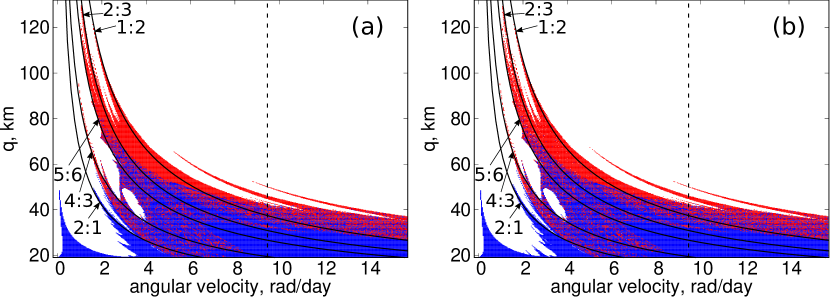
Figure 2: The stability diagrams. (a) Solar perturbations are not taken into account; (b) Solar perturbations are taken into account. Blue domain: particles colliding with the host CB surface; red domain: particles escaping the CB’s Hill sphere; white domain: none of these events taking place in the course of the maximum time interval (1000 yr) of integration. Black solid curves: the locations of several orbit-spin resonances of the orbiting particle with the rotating CB. The dashed vertical line corresponds to the Arrokoth’s current rotation rate, as determined by Porter et al. (2019).

In Rollin, Shevchenko & Lages (2021), we used the physical and dynamical data for Arrokoth as obtained during the New Horizons flyby (Stern et al., 2019a; Cheng et al., 2019; Protopapa et al., 2019; Stern et al., 2019b). To describe the immediate dynamical environments of Arrokoth, we constructed the stability chart, namely, the Lyapunov characteristic exponent (LCE) diagram, in the “pericentric distance – eccentricity” plane $q$–$e$, on a fine grid of initial conditions. The diagram is shown in Figure 2 in Rollin, Shevchenko & Lages (2021), its most prominent feature is the fractal “ragged” border between the chaotic and regular zones. The ragged border is formed by orbit-spin resonances between an orbiting particle and the rotating Arrokoth. The most prominent bands of chaos are formed by the $p/1$ orbit-spin resonances, corresponding to integer ratios of the particle’s orbital period and Arrokoth’s rotation period.

2.2 The 3D problem

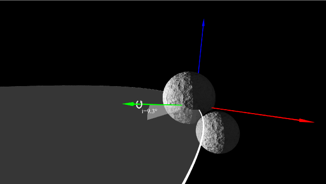
Figure 1: The object scheme and the adopted Arrokoth-centered coordinate system. The axis $z$ (shown in green) of the coordinate system coincides with Arrokoth’s rotation axis. The $x$ and $y$ axes are in red and blue, respectively. Arrokoth’s heliocentric orbit and orbital plane are in white and grey, respectively. The sizes (diameters) of the lobes are $\approx$20 km and $\approx$14 km, and the mean distance from the Sun is $\approx$45 AU.

In the present work, we generalize the dynamical model and explore the dynamical environments of Arrokoth in the 3D setting of the problem, taking into account the actual 3D dynamical parameters of Arrokoth (in particular, its angular momentum vector orientation in space) and gravitational perturbations from the Sun. In Figure 1, the object scheme and the adopted coordinate system are graphically presented.

To describe the dynamical environments of Arrokoth, we construct stability charts in the $q$–$\omega$ (pericentric distance — angular velocity) plane of initial conditions, now in the 3D setting. We choose an inertial Cartesian coordinate system with the origin at the Arrokoth’s mass center. In addition to the gravitational effect of Arrokoth, we take into account perturbations from the distant Sun. The gravitational potential of Arrokoth is considered as a potential of two mass points, the distance between which is constant in time. The $z$-axis of the coordinate system coincides with the spin axis of Arrokoth. The $x$ and $y$ axes complete the $(x,y,z)$ set to an orthogonal one; see Figure 1.

In the general 3D setting, the equations of motion of a passively gravitating particle with radius-vector $\mathbf{r}$ and velocity $\mathbf{v}$ are given by

$$\begin{array}[]{l}\dot{\mathbf{r}}=\mathbf{v},\\ \dot{\mathbf{v}}=-\mathcal{G}m_{1}\frac{\mathbf{r}-\mathbf{r_{1}}}{|\mathbf{r}-\mathbf{r_{1}}|^{3}}-\mathcal{G}m_{2}\frac{\mathbf{r}-\mathbf{r_{2}}}{|\mathbf{r}-\mathbf{r_{2}}|^{3}}+\mathbf{A}_{\mathrm{pert}},\end{array}$$ (3)

where

$$\mathbf{A}_{\mathrm{pert}}=-\mathcal{G}m_{\odot}\frac{\mathbf{r}-\mathbf{r_{\odot}}}{|\mathbf{r}-\mathbf{r_{\odot}}|^{3}}-\mathcal{G}m_{\odot}\frac{\mathbf{r_{\odot}}}{|\mathbf{r_{\odot}}|^{3}}$$ (4)

is the Solar perturbation; $\mathbf{r_{1}}$, $\mathbf{r_{2}}$ and $\mathbf{r_{\odot}}$ are the radius-vectors of Arrokoth’s first and second lobes and the Sun, respectively; $m_{1}$, $m_{2}$ and $m_{\odot}$ are their masses.

We assume that the gravitational influence of the Sun on the spin axis orientation and the rotation rate $\omega$ of Arrokoth is negligible. The locations of the centers of Arrokoth’s two lobes are given by

$$\begin{array}[]{l}\mathbf{r_{1}}=(r_{1}\cos\omega t,r_{1}\sin\omega t,0),\\ \mathbf{r_{2}}=(r_{2}\sin\omega t,r_{2}\cos\omega t,0),\end{array}$$ (5)

where $r_{1}$ and $r_{2}$ are the distances from the CB’s mass center to the mass centers of its lobes.

For a host dumbbell, consisting of two round lobes, as Arrokoth is, the dynamical model given by Equations (3)–(5) is obviously suitable. In vicinities close to the object’s surface, the irregularities of the latter may affect the orbiting particles, especially their accretion onto the object’s surface. However note that any particles with the orbital pericentric distance $q\lesssim 2d$ (where $d$ is the CB’s size) are absorbed by Arrokoth almost immediately (Rollin, Shevchenko & Lages, 2021).

Equations (3)–(5) were integrated by the 15th order Everhart integrator Everhart (1985). The local relative error tolerance was set to $10^{-15}$.

In view of the general scenarios of formation of CB KBOs (Umurhan et al., 2019; McKinnon et al., 2019), we assume, as in Rollin, Shevchenko & Lages (2021), that the post-formation phase of Arrokoth’s evolution starts with the particles initially residing in a disk-like structure formed around the merged CB. In case of Arrokoth, the circumbinary chaotic zone in the disk may extend up to radii $\simeq 6d$ (Rollin, Shevchenko & Lages, 2021). We sampled 400 angular velocity values from 0.01 to 15.78 rad per day; this corresponds to periods from 628.32 d to 9 hr 13 min. The pericentric distances were sampled from 19 km to 130 km with a step of 0.2 km. The parameters of Arrokoth were set as following:

1. The ”dumbbell size” of Arrokoth (the distance between the mass centers of its two lobes): $d=16.1$ km. Radii of the components are $R_{1}=10$ km and $R_{2}=7$ km; see Figure 1 in Cheng et al. (2019). The rotation period of the dumbbell is 15.9 h (Keane et al., 2022).

2. The masses (assuming the density value $\rho=0.5$ g/cm³, typical for cometary nuclei; see Thomas et al. 2013; Jorda et al. 2016) of the lobes are $m_{1}=1.70\cdot 10^{18}$ g and $m_{2}=6.67\cdot 10^{17}$ g (equal to $8.55\cdot 10^{-16}$ and $3.35\cdot 10^{-16}$ in the Solar mass units); therefore, the mass parameter $\mu_{\mathrm{A}}=m_{2}/(m_{1}+m_{2})\approx 0.282$.

3. The Arrokoth’s orbit around the Sun is considered, for our purposes, as circular, as its eccentricity is small ($e_{\mathrm{A}}=0.044$); for the semimajor axis value we set $a_{\mathrm{A}}=44.67$ AU (JPL database, 2022); therefore, the period of motion around the Sun is 298.6 yr.

4. The Arrokoth’s obliquity (the angle between the spin axis of Arrokoth and the normal to its orbital plane) is set to $99.3^{\circ}$, in accordance with data in Porter et al. (2019).

5. The initial eccentricity of the disk particles is set to zero. The particles start orbiting in the Arrokoth’s rotation plane.

6. The computing maximum time is set to 1000 yr, covering $\approx$3.3 Arrokoth’s revolutions around the Sun.

The particle’s orbit is integrated until the computing maximum time is reached or until the particle collides with the asteroid or leaves Arrokoth’s Hill sphere, whose radius is $\approx$50000 km, equal to $\approx 7.5\cdot 10^{-6}$ in units of the radius of Arrokoth’s orbit around the Sun.

The adopted here maximum computing time (1000 yr) is by far sufficient for our current purposes, because the total clearing of the circumbinary chaotic zone takes place on much shorter (by orders of magnitude) timescales, as we find out further on. What is more, the typical orbital periods of particles inside the chaotic zone ($\sim$ hours or days) are also by far shorter.

Concerning Arrokoth’s orbital eccentricity, it is very small $(e\approx 0.04)$, therefore, we do not expect any visible change in the integration results if the eccentricity is taken into account. Further on, we discuss this issue in more detail.

In the resulting diagrams in Figs. 2, we represent graphically the extents of the circum-CB chaotic zone, as determined in our computations, with the Solar perturbations not taken into account (Fig. 2a) and taken into account (Fig. 2b).

The diagrams are defined in the “particle’s initial pericentric distance – CB rotation rate” ($q$–$\omega$) frame. In the diagrams, blue color means that the particle collides with the CB’s surface, red color means that it escapes the CB’s Hill sphere, and white color that none of such events have happened during the maximum (1000 yr) interval of integration. Comparing the diagrams in Fig. 2a and 2b, one finds that in the both considered cases (without and with Solar perturbations) the results are almost identical: the chaos borders are almost the same.

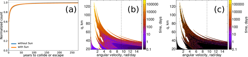
Figure 3: (a) The cumulative distribution for the survival time of particles, in the cases without (blue) and with (yellow) Solar perturbations taken into account. (b) The time to collide or escape as a function of the CB’s angular velocity (rotation rate) and initial perihelion distance. The dashed vertical line marks the Arrokoth’s current angular rotation rate, as determined by Porter et al. (2019). (c) The survival time difference between the cases with and without the Sun.

In Fig. 3a, the cumulative distribution is shown for the time required for a particle to collide with Arrokoth or escape Arrokoth’s Hill sphere. One finds that almost all of the particles collide or escape in 100 yr. A half of the particles has lifetime less than 50 d. No significant differences in results are observed between the two considered cases (with or without the Solar perturbations taken into account). In Fig. 3b, the time needed for a particle to collide with Arrokoth or escape Arrokoth’s Hill sphere as a function of Arrokoth’s initial perihelion distance and rotation rate is presented. Since there are no significant differences, we present solely the case with the Solar perturbations taken into account. Fig. 3c shows the difference in lifetime between the cases with and without the Sun. One may see that the difference is typically much less than the lifetime values themselves (note that the latter are especially large in the upper-left corner of the diagram). However, this inference concerns Arrokoth’s close vicinities covered by the diagram. For much larger orbits, the Solar perturbations become dominant, as discussed further on.

For Arrokoth’s current rotational period, the particles that are closer in orbital radius to Arrokoth’s mass center than 32 km are observed collide with Arrokoth in several days. This is in accord with results by Amarante & Winter (2022). The particles that move initially farther in orbital radius, may collide or escape only if they follow orbits close to orbit-spin resonances (resonances between particle’s orbital period and Arrokoth’s rotation period); therefore, the survival time can generally be much greater.

3 Dispersal of matter around Arrokoth

The diffusion coefficient is as usual defined as the mean-square spread in a selected variable (say, energy $E$), per time unit:

$$D\equiv\lim_{t\to\infty}\frac{\langle(E(t)-E_{0})^{2}\rangle}{t},$$ (6)

where $t$ is time, and the angular brackets denote averaging over a set of starting values of $E$; see Meiss (1992).

As determined in the 2D problem setting (Rollin, Shevchenko & Lages, 2021), for a CB like Arrokoth (with the mass ratio $\mu\sim 0.1$–0.3) the characteristic timescale of the diffusion ($\sim 1/D$) in the immediate circumbinary chaotic zone can be as small as $\sim$10 times CB’s rotation period. This means that the clearing of the chaotic zone is essentially instantaneous. Although this estimate of the transport time was performed in the diffusional approximation, its smallness means that, in fact, the transport is not diffusional, but ballistic (Rollin, Shevchenko & Lages, 2021).

In Rollin, Shevchenko & Lages (2021), the ballistic transport character was shown independently by calculating the amplitude of the kick function for the generalized Kepler map; on the generalized Kepler map theory see Lages, Shepelyansky & Shevchenko (2017); Lages, Shevchenko & Rollin (2018). The kick function in the energy $E$ is given by

$$\Delta E\left(\mu,q,\omega,\phi\right)\simeq W_{1}\left(\mu,q,\omega\right)\sin\left(\phi\right)+W_{2}\left(\mu,q,\omega\right)\sin\left(2\phi\right),$$ (7)

where $\phi$ is the CB’s phase angle when the orbiting particle is at pericenter, and

$$W_{1}\left(\mu,q,\omega\right)\simeq\mu\nu(\nu-\mu)2^{1/4}\pi^{1/2}\omega^{5/2}q^{-1/4}\exp\left(-\frac{2^{3/2}}{3}\omega q^{3/2}\right),$$ (8)

$$W_{2}\left(\mu,q,\omega\right)\simeq-\mu\nu 2^{15/4}\pi^{1/2}\omega^{5/2}q^{3/4}\exp\left(-\frac{2^{5/2}}{3}\omega q^{3/2}\right);$$ (9)

and, by definition, $\nu=1-\mu$.

One may see that, at $\mu\sim 1/3$, $\omega\sim 1$ and $q\sim$2–3 one has $W_{1}\sim W_{2}\sim 1$. Therefore, the single-kick energy variation is $\sim 1$; this means that, indeed, any orbiting particle that is initially placed in the CB’s chaotic zone can be ejected from this zone in a few orbital revolutions (Rollin, Shevchenko & Lages, 2021). This conclusion, obtained in the 2D setting of the problem, is not expected to be subject to change in the 3D setting. However, the statistical behaviour of particles in the removal time distribution tail can be different. We explore this possibility in the following Sections.

4 Cloudization of low-mass matter in the outer orbital zone

According to Rollin, Shevchenko & Lages (2021), the originally formed low-mass matter cocoon inside Arrokoth’s Hill sphere could have suffered $\sim 10$–100 dispersal events since Arrokoth’s formation epoch; therefore, one may expect that Arrokoth’s Hill sphere (as well as Hill spheres of similar KBOs) nowadays is empty.

Recall that the radius $R_{\mathrm{H}}$ of the secondary body’s (say with mass $m_{\mathrm{A}}$) Hill sphere, in units of semimajor axis of the body’s orbit around the primary mass $m_{0}$, is

$$R_{\mathrm{H}}=\left(\frac{\mu}{3}\right)^{1/3},$$ (10)

where $\mu=m_{\mathrm{A}}/(m_{0}+m_{\mathrm{A}})$, as usual, is the mass parameter of the system (here, the Sun–Arrokoth one). The orbit of Arrokoth’s any moonlet should lie within Arrokoth’s Hill sphere. This implies the inequality $a(1+e)\lesssim R_{\mathrm{H}}$, for the semimajor axis $a$ and eccentricity $e$ of the moonlet.

Given the “dumbbell size” of Arrokoth $d=16$ km, it is straightforward to estimate (Rollin, Shevchenko & Lages, 2021) that the chaotic clearing zone around Arrokoth may have radius of at most $\sim$100 km, an order of magnitude less than the New Horizons flyby distance ($\sim$3500 km) and three orders of magnitude less than Arrokoth’s Hill radius ($\sim 5\cdot 10^{4}$ km).

How the low-mass matter cocoon inside the Hill sphere may emerge? As revealed in Tremaine (1993), in any star’s planetary system, there exists a critical semimajor axis at which the chaotic highly-eccentric motion inside the host star’s Hill sphere transforms from the diffusion in energy at approximately constant $q$ to the diffusion in angular momentum at constant energy. This transition takes place where the torque from the Galactic tide starts to dominate. The freezing in energy (equivalently, in semimajor axis) forms an effective barrier for the escape process; thus it is a necessary constituent for the formation of a cocoon of matter inside the Hill sphere.

In the dynamical environments of a contact-binary KBO, quite analogously, the critical radius, at which the diffusion in energy (with the pericentric distance $q$ constant) is stopped and the diffusion in angular momentum (with the semimajor axis $a$ constant) starts, can be estimated by equating the frequency of circumbinary orbital precession to the frequency of the Lidov–Kozai (LK) oscillations. The latter arise due to perturbations from a distant perturber (Lidov, 1961, 1962; Kozai, 1962), the Sun in our case. The criteria for the Lidov–Kozai effect suppression are described in (Shevchenko, 2017, section 3.3). Note that, at the edge of escape of a particle from Arrokoth’s Hill sphere, its orbital period around Arrokoth is $\sim$500 yr, which is greater (by a factor of two) than Arrokoth’s heliocentric orbital period (which is $\approx$300 yr) and is much greater (by five orders of magnitude) than Arrokoth’s rotation period (which is $\approx$16 h); thus allowing one to use averaged equations of motion.

Consider a close binary orbiting the main central mass $m_{0}$ (the Sun in our case, $m_{0}=m_{\odot}$). Thus, we have the primary binary (the Sun–Arrokoth in our case) and the secondary very compact binary (Arrokoth’s two lobes) with masses $m_{1}>m_{2}$; see Figure 1 for a general scheme. The semimajor axes of the primary and secondary binaries are designated henceforth $a_{1}$ and $a_{2}$, respectively; and their eccentricities are $e_{1}$ and $e_{2}$.

Michaely et al. (2017) derived the following formula for estimating the critical semimajor axis value $a_{\mathrm{crit}}$ (below which the Lidov–Kozai effect is suppressed) for a particle orbiting around the secondary binary in such an orbital system:

$$a_{\mathrm{crit}}=\left[\frac{3m_{1}m_{2}\left(1-e_{1}^{2}\right)^{3/2}}{8m_{0}(m_{1}+m_{2})\left(1-e^{2}\right)^{2}}\left|5\cos^{2}i-1\right|\right]^{1/5}\left(a_{1}^{3}a_{2}^{2}\right)^{1/5},$$ (11)

where $e$ and $i$ are the eccentricity and inclination of the particle’s orbit (here the inclination is referred to the orbital plane of the secondary binary), all other quantities are defined as just above, and $e_{2}$ among them is set to zero.

For the Sun–Arrokoth system one has $a_{1}\gg a_{2}$ by many orders of magnitude, whereas the mass of Arrokoth is by many orders of magnitude smaller than the mass of the Sun, $m_{\mathrm{A}}=m_{1}+m_{2}\ll m_{0}$. In our case, the secondary binary is contact, therefore, it is circular, i.e., $e_{2}=0$, as already set above. For a system with $e_{1}\approx 0$ and $i\approx 0^{\circ}$ (as the “Sun–Arrokoth–disk particle” initial configuration is) one may render formula (11) in the form

$$a_{\mathrm{crit}}\approx\left[\frac{3\mu_{1}\mu_{2}a_{1}^{3}a_{2}^{2}}{2\left(1-e^{2}\right)^{2}}\right]^{1/5},$$ (12)

where $\mu_{1}=m_{\mathrm{A}}/(m_{0}+m_{\mathrm{A}})=m_{\mathrm{A}}/m_{0}$ and $\mu_{2}=m_{2}/(m_{1}+m_{2})=m_{2}/m_{\mathrm{A}}$ are, respectively, the mass parameters of the primary and secondary binaries in our system; $m_{0}$, $m_{1}$, and $m_{2}$ are, respectively, the masses of the Sun and Arrokoth’s lobes ($m_{1}>m_{2}$); $a_{1}$ and $a_{2}$ are, respectively, Arrokoth’s orbital semimajor axis (of the orbit around the Sun) and Arrokoth’s dumbbell size; $e_{1}=0.04\simeq 0$ is the eccentricity of Arrokoth’s orbit around the Sun.

The obliquity of the secondary binary’s orbital plane (the dumbbell’s rotation plane, in the given case) with respect to the primary binary’s orbit is assumed to be high enough, so that the Lidov–Kozai effect for particles orbiting around Arrokoth in the plane of its rotation is potentially present (at $a>a_{\mathrm{crit}}$). Note that the obliquity of Arrokoth’s rotation plane is indeed high, $\sim 99^{\circ}$ (Porter et al., 2019), as needed.

For the necessary quantities to substitute in Equation (12), one has: $\mu_{1}\approx 1.19\cdot 10^{-15}$, $\mu_{2}\approx 0.28$, $a_{1}=44.54$ AU $\approx 6.68\cdot 10^{14}$ cm, $a_{2}=d\approx 1.6\cdot 10^{6}$ cm, and we formally set $e=0$. Substituting the values of all these quantities in Equation (12), one finds $a_{\mathrm{crit}}\simeq 2100$ km. Due to the specific dependence of $a_{\mathrm{crit}}$ on $e$, the $a_{\mathrm{crit}}$ value is by the order of magnitude the same for circular and eccentric orbits, even at large $e$ values. As soon as $R_{\mathrm{H}}\simeq 10^{5}$ km, we find that $a_{\mathrm{crit}}\ll R_{\mathrm{H}}$.

One may thus be confident that the particles’ random walk in energy is effectively frozen already deep inside the Hill sphere, and the low-mass matter cocoon may indeed be formed by particles leaving the circumbinary chaotic zone, as well as by any low-mass material initially residing in regular orbits in the outer parts of the circumbinary disk.

Such material can be effectively “cloudized,” i.e., converted from the planar disk to a non-planar, approximately spherically-symmetric cloud. Indeed, at $a>a_{\mathrm{crit}}$, the Lidov–Kozai effect is not suppressed; therefore, the highly-eccentric particles may suffer the LK-oscillations in their eccentricity and inclination. Let us approximately estimate the cloudization timescale.

As above, we assume the CB to move in a circular ($e_{1}=0$) orbit of radius $a_{1}$ around the Sun. For the Keplerian orbital elements of a particle orbiting around the CB (in the plane of its rotation) we take, as usual, the semimajor axis, eccentricity, inclination, argument of pericenter, longitude of ascending node, and mean anomaly, denoted by $a$, $e$, $i$, $\omega$, $\Omega$, and $M$, respectively.

In any two-body problem, the Delaunay variables are defined as (see, e.g., Morbidelli 2002; Shevchenko 2017)

$$\begin{array}[]{lclcl}L&=&[\mathcal{G}(m^{\prime}+m^{\prime\prime})a]^{1/2},&l&=M,\\ G&=&L(1-e^{2})^{1/2},&g&=\omega,\\ H&=&G\cos i,&h&=\Omega,\\ \end{array}$$ (13)

where $m^{\prime}$ and $m^{\prime\prime}$ are the two masses, and $\mathcal{G}$ is the gravitational constant. The variables $L$ and $l$, $G$ and $g$, $H$ and $h$ form three pairs of conjugate canonical variables. $L$ is a function of the semimajor axis solely and thus can be expressed through the orbital energy; $G$ is the absolute value of the reduced (per unit of mass) angular momentum; and $H$ is the reduced angular momentum vector’s vertical component. Therefore, $G$ is the specific angular momentum, and its time derivative $\dot{G}$ is the torque (per unit of mass).

In the presence of a perturbing third body in an outer orbit, the equation for the Lidov–Kozai evolution of the angular momentum $G$ of the inner binary is given by

$$\dot{G}=-\frac{15\mathcal{G}m_{\mathrm{pert}}a^{2}}{8a_{\mathrm{pert}}^{3}}e^{2}\sin^{2}i\sin 2\omega$$ (14)

(Shevchenko, 2017, Equation 3.26), where $m_{\mathrm{pert}}$ is the mass of the perturber. In our problem, the perturber is the Sun, therefore, $m_{\mathrm{pert}}=m_{0}$, $a_{\mathrm{pert}}=a_{1}$. Here Arrokoth is considered as a single gravitating point (because the particle’s orbit is assumed to be large enough), and the particle’s orbital inclination is referred to the primary binary’s orbital plane.

At present, Arrokoth’s rotation plane is inclined by $\approx 99^{\circ}$ with respect to the ecliptic plane (Porter et al., 2019), i.e., the obliquity is extremal. Therefore, we set $\sin i\simeq 1$ here. Also setting $e\simeq 1$ (since our particles are highly eccentric) and substituting $|\sin 2\omega|$ by its averaged (over an ensemble of particles) value $2/\pi$, we obtain

$$|\langle\dot{G}\rangle|=\frac{15\mathcal{G}m_{\mathrm{pert}}a^{2}}{4\pi a_{\mathrm{pert}}^{3}}.$$ (15)

Let us define the characteristic timescale for the Lidov–Kozai evolution as the time needed for $G$ to change by of order of itself. This is just the characteristic time needed to convert the initial ring (with radius $a$) of particles to a spherical cloud, i.e., to make the initial planar distribution 3D-isotropic; we designate this time $T_{\mathrm{3D}}$.

For a highly-eccentric passively gravitating particle, the reduced angular momentum is given by

$$G=\left[\mathcal{G}m_{\mathrm{CB}}a(1-e^{2})\right]^{1/2}\simeq(2\mathcal{G}m_{\mathrm{CB}}q)^{1/2}$$ (16)

(see Equations (LABEL:var_D)), where $m_{\mathrm{CB}}$ is the CB’s mass (the mass of Arrokoth, in our case), and $a$, $e$, $q$ are the test particle’s semimajor axis, eccentricity and pericentric distance, respectively. Equating $|\langle\dot{G}\rangle|\simeq G/T_{\mathrm{3D}}$, one obtains

$$T_{\mathrm{3D}}\simeq\frac{2^{5/2}\pi}{15}\,\frac{m_{\mathrm{CB}}^{1/2}a_{\mathrm{pert}}^{3}}{\mathcal{G}^{1/2}m_{\mathrm{pert}}}\,\frac{q^{1/2}}{a^{2}}.$$ (17)

Substituting $m_{\mathrm{CB}}=m_{\mathrm{Arrokoth}}\simeq 2.37\cdot 10^{18}$ g, $m_{\mathrm{pert}}=m_{0}=1.989\cdot 10^{33}$ g, $a_{\mathrm{pert}}=a_{1}=44.54$ AU$\approx 6.68\cdot 10^{14}$ cm, $q=$(2–5) $d_{\mathrm{Arrokoth}}=$(3.2–8.0)$\cdot 10^{6}$ cm, $a=R_{\mathrm{H}}\sim 10^{10}$ cm, one has: $T_{\mathrm{3D}}\sim 0.6$–0.9 yr.

Given that, for a particle orbiting around Arrokoth with the semimajor axis $a\sim R_{\mathrm{H}}\sim 10^{5}$ km, the orbital period is $\sim 500$ yr, we see that the conversion process of the periphery of the initial disk of particles to a spherical cloud, if assessed in the orbital timescale, should be relatively rapid. In what concerns the disk’s inner zone, most of the particles escape or are absorbed by Arrokoth in just a few revolutions around the CB.

In Fig. 4, the evolution of the orbital inclination of particles with time is illustrated, as observed in our numerical experiments. The particles were set to initially have circular orbits with various values of the radius, in the plane orthogonal to the spin axis of Arrokoth. In the Figure, the curves of different colours (blue, orange and green) correspond to three different initial values of the semimajor axis; these values are indicated at each panel. The integration of motion is performed in the same way as described in Section 2, but with the time limit of 250000 yr; the CB’s rotation rate is set equal to the current one. The integrated orbits demonstrate that the particles with semimajor axes greater than 16000 km do not survive on times greater than 50000 yr. The particles with smaller semimajor axes are mostly long-lived.

In Figs. 5–8, we present, for completeness of the dynamical picture, the concurrent time evolution of several other than inclination important orbital elements: eccentricity, semimajor axis, pericentric and apocentric distances. As in Fig. 4, the curves of different colours (blue, orange and green) correspond to three different initial values of the semimajor axis.

From Figs. 4–8 it follows that the numerically observed timescales of cloudization of the outer orbital zone are in accord with our theoretical estimates, based on consideration of Solar perturbations, as provided by Eqs. 17; indeed, the orbital inclinations, in the outer zone, rise macroscopically already on the scale of Arrokoth’s period of motion around the Sun.

In Figs. 4–5 and 7–8, the Lidov–Kozai oscillations are readily recognizable, especially clearly in the middle panels of these plots. What is more, as one may deduce from the first (top left) panels, the Lidov–Kozai effect is indeed suppressed at the orbital radii less than $\sim$2000 km, in accord with our prediction made above using Equation (12): no definite LK-oscillations emerge if $a_{0}$ is smaller than $\sim$2000 km.

According to (Shevchenko, 2017, section 3.2.2), the quantity

$$c_{1}=(1-e^{2})\cos^{2}i=\mathrm{const},$$ (18)

is conserved during the Lidov–Kozai oscillations, i.e., the vertical component of the angular momentum squared is constant. This relation implies that, if $0\leq i\leq\pi/2$, then the secular variations of $e$ and $i$ are coupled in anti-phase; whereas, if $\pi/2\leq i\leq\pi$, then the variations of $e$ and $i$ are coupled in phase. The eccentricity is maximum at $i=0$, and the inclination is maximum at $e=0$. If the initial inclination $i_{0}$ is greater than a critical value ($\sim 40^{\circ}$; see Shevchenko 2017 for review and details), then the maximum eccentricity value is essentially insensitive to the value of $e_{0}$ (if $e_{0}\lesssim 0.1$) and can be estimated by means of the formula

$$e_{\mathrm{max}}\approx\left(1-\frac{5}{3}\cos^{2}i_{0}\right)^{1/2}$$ (19)

(Holman, Touma, & Tremaine, 1997; Innanen et al., 1997).

In the Lidov–Kozai theory, the time-averaged semimajor axis is constant with time. As one may see in Fig. 6, the semimajor axis is indeed approximately conserved on long intervals of time, but sometimes it exhibits small jumps. The cause of these fluctuations is as follows. According to Equation (19), if the initial $i_{0}\sim 90^{\circ}$ (as in the given case), in the course of LK-oscillations the eccentricity varies almost in the whole interval from zero to unity; this means that the pericentric distance periodically goes down to almost zero, and thus, from time to time, the particle approaches the central rotating dumbbell and receives, in accord with the Kepler map theory (Shevchenko, 2011; Lages, Shepelyansky & Shevchenko, 2017, 2018), a kick in energy, which depends on the approach distance and the dumbbell’s orientation, when the particle is at its orbital pericentre. The energy kick affects the semimajor axis; therefore, the character of the following LK-oscillations is modified, but is being sustained until the next close approach to the CB takes place.

The fact that, in the course of the LK-oscillations, the eccentricity varies here almost in the whole interval from zero to unity means that the particle periodically approaches the parabolic separatrix (the border between the elliptic and hyperbolic types of motion) and thus, due to perturbations, may easily become unbound. This explains the observed (in Figs. 4–8) rapid removal of the low-mass matter from the disk at the radii $\gtrsim$2000 km, where the LK-oscillations are not suppressed.

On the other hand, as we have found out in Section 3, at radii $\lesssim$100 km the disk is rapidly cleared because, if close enough to the rotating dumbbell, the motion is chaotic. Therefore, solely the material that has initial orbital radii in the interval from $\sim$100 to $\gtrsim$2000 km may survive.

At the LK-resonance center, for a massless particle with orbital period $P_{\mathrm{orb}}$ and semimajor axis $a$ (all other notations are as adopted above) the period of LK-oscillations can be rendered in the form

$$P_{\mathrm{LK}}\approx P_{\mathrm{orb}}\frac{m_{\mathrm{A}}}{m_{0}}\left(\frac{a_{1}}{a}\right)^{3}(1-e_{1}^{2})^{3/2}$$ (20)

(Mazeh & Shaham, 1979; Holman, Touma, & Tremaine, 1997; Shevchenko, 2017). The periods of patterns in Figs. 4–5 and 7–8 are in accord with Equation (20). E.g., according to Fig. 5, the quasiperiodic eccentricity variations, where they can be effectively identified, have the time periods of $\sim$10000 yr (at $a_{0}=$4000, 6000 and 8000 km) and $\sim$1000 yr (at $a_{0}=$21500, 22000 and 24000 km), and the same approximate values are respectively produced by Equation (20), as one may straightforwardly verify.

How principal is the circular approximation for Arrokoth’s orbit around the Sun? Setting $e_{1}=0.044$ (for Arrokoth’s actual elliptic orbit), instead of $e_{1}=0$ in Equation (20), results in a difference in $P_{\mathrm{LK}}$ of only $\sim$0.2%; therefore, taking into account Arrokoth’s eccentricity is of no importance for our estimates, which are made by the order of magnitude. Besides, the smallness of this difference shows that the eccentricity is as well essentially unimportant in numerical integrations (of the kind presented in previous Sections), when one is interested in the general dynamics character.

As a graphical illustration of the “cloudization” phenomenon, an attached animation and its two snapshots (Fig. 9) demonstrates how an initial planar ring of particles evolves, in the course of time, into a complex 3D aggregate, arising due to Solar perturbations. In this simulation, 1000 particles were initially placed in circular orbits with initial radii ranging from $r_{\rm min}=20000$ km to $r_{\rm max}=23000$ km. The simulation was performed over 10000 yr; this is a typical time range as used above to construct Figs. 4–8.

Fig. 9, right panel, exhibits the evolved 3D aggregate as formed to the moment $t=5470$ yr (chosen here as a representative one); the left panel demonstrates the initial particle distribution. The evolved semimajor axes $a$ of the particles’ orbits are mostly distributed in the range 20000–26000 km; however, in the course of evolution, some particles achieved $a>R_{\mathrm{H}}$ and escaped (and were therefore removed from the computation), in agreement with Figs. 4–8. Furthermore, the eccentricity distribution rapidly becomes uniform, whereas the inclination distribution shows broad peaks whose number and locations vary with time. Analysis of these complex spatial structures will be conducted elsewhere in further studies.

5 Conclusions

In this article, we have considered dynamical environments of (486958) Arrokoth, focusing on both their present state and their long-term evolution, starting from the epoch of formation of the object.

Both analytical (based on an upgraded Kepler-map formalism) and numerical (based on massive simulations and construction of stability diagrams) approaches to the problem have been used.

Our main conclusions are as following.

• In the 3D setting, the clearing process of the chaotic circumbinary zone is practically instantaneous, as it is in the planar case (explored in Rollin, Shevchenko & Lages 2021).

• In the inner orbital zone (closer than 130 km to Arrokoth) most of the particles (more than $\approx$60%) that collide with Arrokoth or escape its Hill sphere do it in $\sim$50 d. For Arrokoth with its current rotation rate, the particles with initial orbital radius less than 32 km collide with Arrokoth in several days. For more distant ones, this takes up to $\sim$10–100 yr.

• The numerically observed timescales of cloudization of the outer orbital zone are in accord with theoretical estimates, based on consideration of Solar perturbations, as demonstrated and discussed above in Section 4.

• In the outer orbital zone, the particles that are initially farther than $\sim$18000 km from Arrokoth cannot survive due to Solar perturbations. The particles that are initially farther from Arrokoth than $\sim$100 km and closer than $\sim$18000 km are mostly stable.

• The generic chaotization of Arrokoth’s circumbinary debris disk’s inner zone and generic cloudization of the disk’s periphery, showed by us to be essential in the general 3D case, naturally explains the current absence of any debris in its vicinities.

Acknowledgments. The authors are most thankful to Gustavo Madeira for valuable remarks and comments. I.I.S. was supported in part by the Russian Science Foundation, project 22-22-00046.

Data availability. The data underlying this article will be shared on reasonable request to the corresponding author.

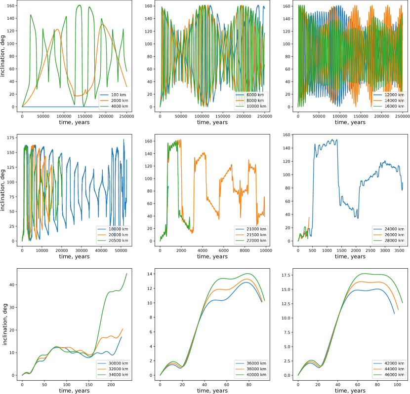
Figure 4: Orbital inclination of a particle as a function of time at various initial orbital semimajor axes. Initially the particle is placed in a circular orbit in the plane orthogonal to Arrokoth’s spin axis.

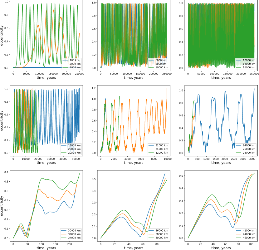
Figure 5: The same as Fig. 4, but for eccentricity.

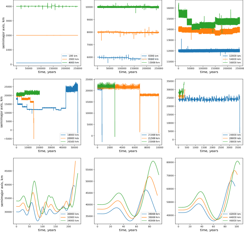
Figure 6: The same as Fig. 4, but for semimajor axis. The semimajor axis excursions to negative values take place when the orbit becomes hyperbolic, and the particle escapes.

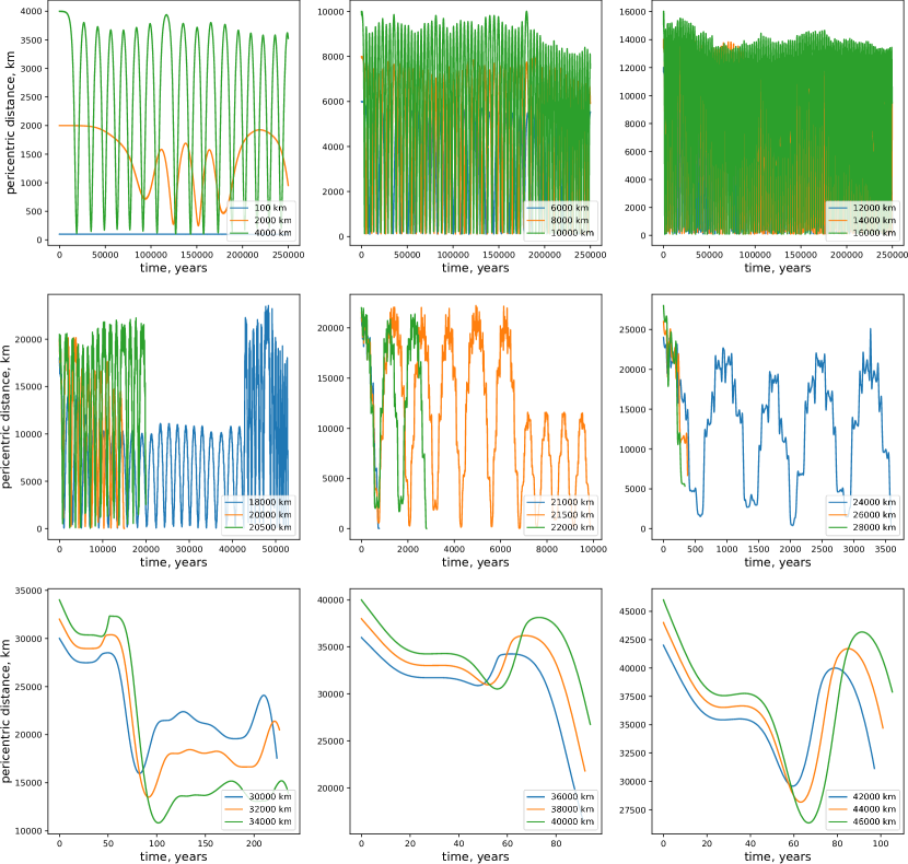
Figure 7: The same as Fig. 4, but for pericentric distance.

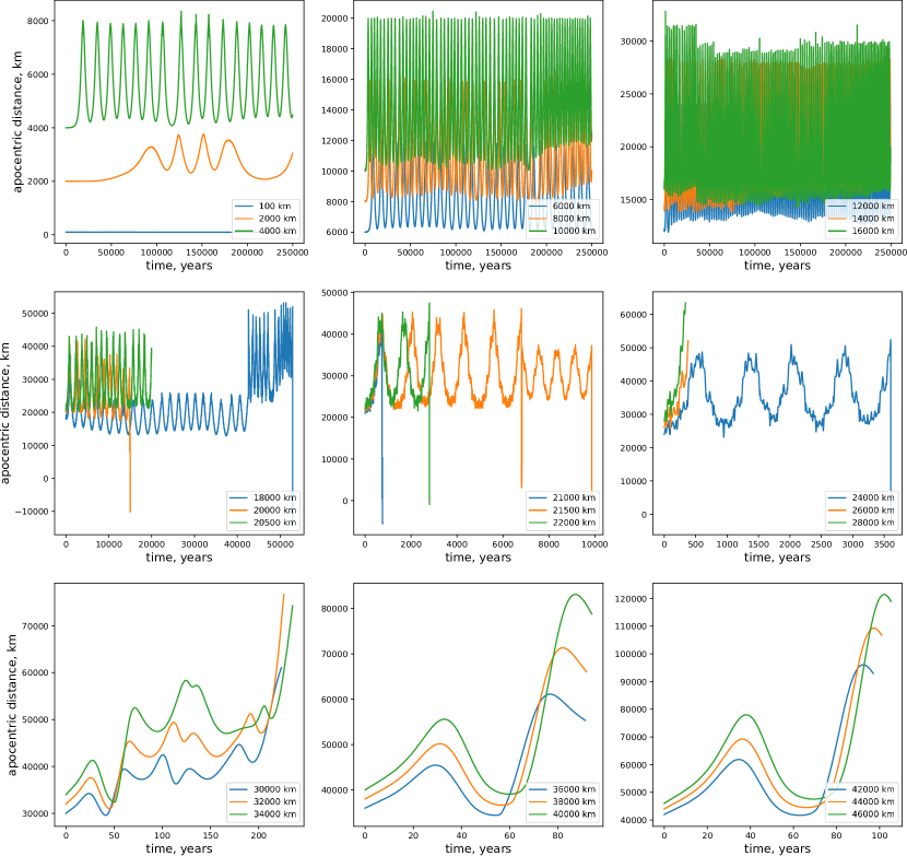
Figure 8: The same as Fig. 4, but for apocentric distance.

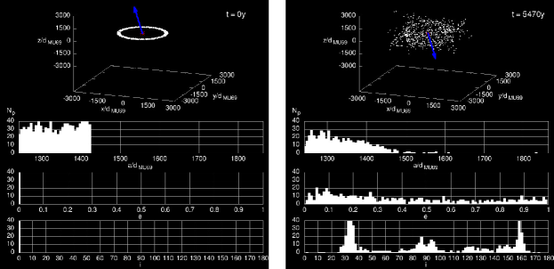
Figure 9: Two snapshots (at time moments $t=0$ and $t=$5470 yr) of the particles’ cloud 3D evolution around Arrokoth. The initial (at $t=0$) ring of the particles lies in the plane almost orthogonal (inclination 99^∘) to Arrokoth’s spin axis. The mass parameter $\mu=0.28$. The blue arrows give the direction to the Sun during the simulation. The complete animation of the evolution can be found at https://search-data.ubfc.fr/FR-13002091000019-2022-08-05_Dynamical-environments-of-Arrokoth-prior.html

References

- Amarante & Winter (2022) Amarante A., Winter O. C., 2022, Ap&SS, 367, 38
- Cheng et al. (2019) Cheng A. F., et al., 2019, in: 50th Lunar and Planetary Science Conference 2019, LPI Contrib. No. 2132, id. 3273
- Everhart (1985) Everhart E., 1985, in: Carusi A., & Valsecchi G. B., eds, IAU Colloq. 83, Dynamics of Comets: Their Origin and Evolution, v. 115, p. 185
- Gladstone et al. (2019) Gladstone G. R., et al., 2019, in: 50th Lunar and Planetary Science Conference 2019, LPI Contrib. No. 2132, id. 2866