Generalization Bounds for Adversarial Contrastive Learning

Abstract

Deep networks are well-known to be fragile to adversarial attacks, and adversarial training is one of the most popular methods used to train a robust model. To take advantage of unlabeled data, recent works have applied adversarial training to contrastive learning (Adversarial Contrastive Learning; ACL for short) and obtain promising robust performance. However, the theory of ACL is not well understood. To fill this gap, we leverage the Rademacher complexity to analyze the generalization performance of ACL, with a particular focus on linear models and multi-layer neural networks under $\ell_{p}$ attack ($p\geq 1$). Our theory shows that the average adversarial risk of the downstream tasks can be upper bounded by the adversarial unsupervised risk of the upstream task. The experimental results validate our theory.

Keywords: Robustness, Adversarial learning, Contrastive learning, Rademacher complexity, Generalization bound.

1 Introduction

Deep neural networks (DNNs) have achieved state-of-the-art performance in many fields. However, several prior works (Szegedy et al., 2014; Goodfellow et al., 2015) have shown that DNNs may be vulnerable to imperceptibly changed adversarial examples, which causes a lot of focus on the robustness of the models (Madry et al., 2018; Mao et al., 2020; Li et al., 2022).

One of the most popular approaches to achieving adversarial robustness is adversarial training, which involves training the model with samples perturbed to maximize the loss on the target model (Goodfellow et al., 2015; Madry et al., 2018; Zhang et al., 2019). Schmidt et al. (2018) show that adversarial robust generalization requires a larger amount of data, while Yin et al. (2019); Awasthi et al. (2020) show that the Rademacher Complexity of adversarial training is strictly larger in theory than that of natural training, which implies that we need more data for adversarial training.

Since the labeled data is limited and expensive to obtain, one option would be to use large-scale unlabeled data and apply self-supervised learning (Gidaris et al., 2018; Noroozi and Favaro, 2016), an approach that trains the model on unlabeled data in a supervised manner by utilizing self-generated labels from the data itself. Contrastive Learning (CL) (Chen et al., 2020; He et al., 2020), which aims to maximize the feature similarity of similar pairs and minimize the feature similarity of dissimilar ones, is a popular self-supervised learning technique.

Recently, Kim et al. (2020); Ho and Vasconcelos (2020); Jiang et al. (2020) apply adversarial training in CL and achieve state-of-the-art model robustness. They find that if adversarial training is conducted on the upstream contrastive task, the trained model will be robust on the downstream supervised task. However, their results are all empirical and lack theoretical analysis. To fill this gap, we here present a theoretical analysis of adversarial contrastive learning through the lens of Rademacher complexity, with a particular focus on linear models and multi-layer neural networks. Our theoretical results show that the average adversarial risk of the downstream tasks can be upper bounded by the adversarial unsupervised risk of the upstream task; this implies that if we train a robust feature extractor on the upstream task, we can obtain a model that is robust on downstream tasks.

The remainder of this article is structured as follows: §2 introduces some related works in this field. §3 provides some basic definitions and settings that will be used in the following sections. §4 presents our first part’s main results, which show a connection between the robust risk for the upstream task and the robust risk for the downstream tasks. §5 shows our second part’s results, it outlines our bounds for linear models and multi-layer neural networks by bounding the Rademacher complexity of each hypothesis class. §6 shows some experimental results that verify our theory; finally, the conclusions are presented in the last section.

2 Related Work

Adversarial Robustness. Szegedy et al. (2014) show that DNNs are fragile to imperceptible distortions in the input space. Subsequently, Goodfellow et al. (2015) propose the fast gradient sign method (FGSM), which perturbs a target sample towards its gradient direction to increase the loss and then uses the generated sample to train the model in order to improve the robustness. Following this line of research, Madry et al. (2018); Moosavi-Dezfooli et al. (2016); Kurakin et al. (2017); Carlini and Wagner (2017) propose iterative variants of the gradient attack with improved adversarial learning frameworks. Besides, Ma et al. (2022) analyze the trade-off between robustness and fairness, Li and Liu (2023) study the worst-class adversarial robustness in adversarial training. For the theoretical perspective, Montasser et al. (2019) study the PAC learnability of adversarial robust learning, Xu and Liu (2022) extend the work of Montasser et al. (2019) to multiclass case and Yin et al. (2019); Awasthi et al. (2020) give theoretical analysises to adversarial training by standard uniform convergence argumentation and giving a bound of the Rademacher complexity. Our work is quite different from Yin et al. (2019); Awasthi et al. (2020), firstly, they just analyze the linear models and two-layer neural networks, but we consider linear models and multi-layer deep neural networks; secondly, they consider the classification loss, which is much easier to analyze than our contrastive loss.

Contrastive Learning. Contrastive Learning is a popular self-supervised learning paradigm that attempts to learn a good feature representation by minimizing the feature distance of similar pairs and maximizing the feature distance of dissimilar pairs (Chen et al., 2020; Wang and Liu, 2022). SimCLR (Chen et al., 2020) learns representations by maximizing the agreement between differently augmented views of the same data, while MoCo (He et al., 2020) builds large and consistent dictionaries for unsupervised learning with a contrastive loss. From the theoretical perspective, Saunshi et al. (2019) first presents a framework to analyze CL. We generalize their framework to the adversarial CL. The key challenging issues in this work are how to define and rigorously analyze the adversarial CL losses. Moreover, we further analyze the Rademacher complexity of linear models and multi-layer deep neural networks composited with a complex adversarial contrastive loss. Neyshabur et al. (2015) show an upper bound of the Rademacher complexity for neural networks under group norm regularization. In fact, the Frobenius norm and the $\ell_{1,\infty}$-norm in our theoretical analysis are also group norms, while the settings and proof techniques between Neyshabur et al. (2015) and our work are quite different: (1) they consider the standard setting while we consider a more difficult adversarial setting; (2) they consider the Rademacher complexity of neural networks with size $1$ output layer, while we consider the case that the neural network is composited with a complex contrastive learning loss; (3) they prove their results by reduction with respect to the number of the layers, while motivated by the technique of Gao and Wang (2021), we use the covering number of the neural network to upper bound the Rademacher complexity in the adversarial case.

Adversarial Contrastive Learning. Several recent works (Kim et al., 2020; Ho and Vasconcelos, 2020; Jiang et al., 2020) apply adversarial training in the contrastive pre-training stage to improve the robustness of the models on the downstream tasks, achieving good robust performance in their experiments. Our work attempts to provide a theoretical explanation as to why models robustly trained on the upstream task can be robust on downstream tasks.

3 Problem Setup

We introduce the problem setups in this section.

3.1 Basic Contrastive Learning Settings

We first set up some notations and describe the contrastive learning framework.

Let $\mathcal{X}\in\mathbb{R}^{m}$ be the domain of all possible data points, this paper assumes that $\mathcal{X}$ is bounded. Contrastive learning assumes that we get the similar data in the form of pairs $(x,x^{+})$, which is drawn from a distribution $\mathcal{D}_{sim}$ on $\mathcal{X}^{2}$, and $k$ independent and identically distributed (i.i.d.) negative samples $x_{1}^{-},x_{2}^{-},\dots,x_{k}^{-}$ drawn from a distribution $\mathcal{D}_{neg}$ on $\mathcal{X}$. Given the training set $\mathcal{S}=\{(x_{i},x_{i}^{+},x_{i1}^{-},\dots,x_{ik}^{-})\}_{i=1}^{M}$, we aim to learn a representation $f$ from $\mathcal{F}$ that maps similar pairs $(x,x^{+})$ into similar points $(f(x),f(x^{+}))$, while at the same time keeping $f(x_{i}^{-}),\cdots,f(x_{k}^{-})$ away from $f(x)$, where $\mathcal{F}$ is a class of representation functions $f:\mathcal{X}\to\mathbb{R}^{n}$.

Latent Classes. Let $\mathcal{C}$ denote the set of all latent classes (Saunshi et al., 2019) that are all possible classes for points in $\mathcal{X}$; for each class $c\in\mathcal{C}$ , moreover, the probability $\mathcal{D}_{c}$ over $\mathcal{X}$ captures the probability that a point belongs to class $c$. The distribution on $\mathcal{C}$ is denoted by $\rho$.

To formalize the similarity among data in $\mathcal{X}$, assume we obtain i.i.d. similar data points $x,x^{+}$ from the same distribution $\mathcal{D}_{c}$, where c is randomly selected according to the distribution $\rho$ on latent classes $\mathcal{C}$. We can then define $\mathcal{D}_{sim}$ and $\mathcal{D}_{neg}$ as follows:

Definition 1 ($\mathcal{D}_{sim}$ and $\mathcal{D}_{neg}$, Saunshi et al., 2019)

For unsupervised tasks, we define the distribution of sampling similar samples $\mathcal{D}_{sim}(x,x^{+})$ and negative sample $\mathcal{D}_{neg}(x^{-})$ as follows:

$$\mathcal{D}_{sim}(x,x^{+})=\underset{c\sim\rho}{\mathbb{E}}\mathcal{D}_{c}(x)\mathcal{D}_{c}(x^{+}),\ \ \mathcal{D}_{neg}(x^{-})=\underset{c\sim\rho}{\mathbb{E}}\mathcal{D}_{c}(x^{-}).$$

Supervised Tasks. For supervised tasks, we focus on the tasks in which a representation function $f$ will be tested on a $(k+1)$-way supervised task $\mathcal{T}$ consisting of distinct classes $\{c_{1},c_{2},\dots,c_{k+1}\}\subseteq\mathcal{C}$, while the labeled data set of task $\mathcal{T}$ consists of $M$ i.i.d. examples drawn according to the following process: A label $c\in\{c_{1},\dots,c_{k+1}\}$ is selected according to a distribution $\mathcal{D}_{\mathcal{T}}$, and a sample $x$ is drawn from $\mathcal{D}_{c}$. The distribution of the labeled pair $(x,c)$ is defined as: $\mathcal{D}_{\mathcal{T}}(x,c)=\mathcal{D}_{\mathcal{T}}(c)\mathcal{D}_{c}(x)$.

3.2 Evaluation Metric for Representations

We evaluate the quality of a representation function $f$ with reference to its performance on a multi-class classification task $\mathcal{T}$ using a linear classifier.

Consider a task $\mathcal{T}=\{c_{1},\dots,c_{k+1}\}$. A multi-class classifier for $\mathcal{T}$ is a function $g:\mathcal{X}\xrightarrow[]{}\mathbb{R}^{k+1}$, the output coordinates of which are indexed by the classes $c$ in task $\mathcal{T}$.

Let $\{g(x)_{y}-g(x)_{y^{\prime}}\}_{y^{\prime}\neq y}$ be a $k$-dimensional vector of differences in the coordinates of the output of the classifier $g$. The loss function of $g$ on a point $(x,y)\in\mathcal{X}\times\mathcal{T}$ is defined as $\ell(\{g(x)_{y}-g(x)_{y^{\prime}}\}_{y^{\prime}\neq y})$. For example, one often considers the standard hinge loss $\ell(\boldsymbol{v})=\max\{0,1+\max_{i}\{-\boldsymbol{v}_{i}\}\}$ and the logistic loss $\ell(\boldsymbol{v})=log_{2}(1+\sum_{i}exp(-\boldsymbol{v}_{i}))$ for $\boldsymbol{v}\in\mathbb{R}^{k}$.

The supervised risk of classifier $g$ is defined as follows:

$$L_{sup}(\mathcal{T},g)\coloneqq\underset{(x,c)\sim\mathcal{D}_{\mathcal{T}}}{\mathbb{E}}\left[\ell\left(\left\{g(x)_{c}-g(x)_{c^{\prime}}\right\}_{c^{\prime}\neq c}\right)\right].$$

The risk $L_{sup}(\mathcal{T},g)$ of classifier $g$ on task $\mathcal{T}$ measures the quality of the outputs of $g$, take the hinge loss as an example, our goal is to get a classifier that has much higher confidence for the true class (i.e., the value $g(x)_{c}$) than others (i.e., the values $g(x)_{c^{\prime}}$ for $c^{\prime}\neq c$), so we want all the differences $g(x)_{c}-g(x)_{c^{\prime}}$ for $c\neq c^{\prime}$ to be as large as possible. If $g$ wrongly classifies $x$, i.e., $\underset{c^{\prime}}{\arg\max}g(x)_{c^{\prime}}\neq c$, of course, $\ell$ on $(x,c)$ is not smaller than $1$; however, even thought $g$ correctly classifies $x$, the loss value can not decrease to zero unless $g(x)_{c}-g(x)_{c^{\prime}}\geq 1$ for all $c^{\prime}\neq c$.

Let $\{c_{i}\}_{i=1}^{k+1}=\{c_{1},\dots,c_{k+1}\}$ be a set of classes from $\mathcal{C}$. Given the matrix $W\in\mathbb{R}^{(k+1)\times n}$, we have $g(x)=Wf(x)$ as a classifier that composite the feature extractor $g$ and linear classifier $W$. The supervised risk of $f$ is defined as the risk of $g$ when the best $W$ is chosen:

$$L_{sup}(\mathcal{T},f)\coloneqq\underset{W\in\mathbb{R}^{(k+1)\times n}}{\inf}L_{sup}(\mathcal{T},Wf).$$

When training a feature extractor $f$ on the upstream task, we do not make predictions on the examples, so we can’t define the risk of the feature extractor $f$ as we do for the classifier $g$. Our goal on the upstream task is to train a feature extractor that can perform well on the downstream tasks, so we consider the potential of the feature extractor here, i.e., the minimal possible classification risk of a linear classifier on the feature extracted by $f$. So we define the risk of the feature extractor $f$ as above by taking the infimum over all linear classifiers.

Definition 2 (Mean Classifier, Saunshi et al., 2019)

For a function $f$ and task $\mathcal{T}=\{c_{1},\dots,c_{k+1}\}$, the mean classifier is $W^{\mu}$, whose $c^{th}$ row is the mean $\mu_{c}\coloneqq\underset{x\sim\mathcal{D}_{c}}{\mathbb{E}}[f(x)]$ and we define $L_{sup}^{\mu}(\mathcal{T},f)\coloneqq L_{sup}(\mathcal{T},W^{\mu}f)$.

Since $L_{sup}(\mathcal{T},f)$ involves taking infimum over all possible linear classifiers, it is difficult to analyze $L_{sup}(\mathcal{T},f)$ and establish connections between the risk of the unsupervised upstream task and $L_{sup}(\mathcal{T},f)$. We introduce the mean classifier to bridge them by bounding average $L_{sup}^{\mu}(\mathcal{T},f)$ over the tasks with the risk of the unsupervised upstream risk (for more details, please refer to §4).

Definition 3 (Average Supervised Risk)

The average supervised risk for a function $f$ on $(k+1)$-way tasks is defined as:

$$L_{sup}(f)\coloneqq\underset{\{c_{i}\}_{i=1}^{k+1}\sim\rho^{k+1}}{\mathbb{E}}[L_{sup}(\{c_{i}\}_{i=1}^{k+1},f)|c_{i}\neq c_{j}]$$

Given the mean classifier, the average supervised risk for a function $f$ is defined as follows:

$$L_{sup}^{\mu}(f)\coloneqq\underset{\{c_{i}\}_{i=1}^{k+1}\sim\rho^{k+1}}{\mathbb{E}}[L_{sup}^{\mu}(\{c_{i}\}_{i=1}^{k+1},f)|c_{i}\neq c_{j}].$$

In contrastive learning, the feature extractor is trained as a pretrained model to be used on downstream tasks. There may be many different downstream tasks such as binary classification tasks with classes $\{c_{1},c_{2}\}\subseteq\mathcal{C}$ and many other multi-class classification tasks, so here we consider the average error of $L_{sup}^{\mu}(\mathcal{T},f)$ over all possible tasks $\mathcal{T}$ sampled from $\rho^{k+1}$ as the final performance measure of a feature extractor $f$.

3.3 Contrastive Learning Algorithm

We denote $k$ as the number of negative samples used for training and $(x,x^{+})\!\!\sim\!\!\mathcal{D}_{sim}$, $(x_{1}^{-},\dots,x_{k}^{-}\!)\!\!\sim\!\!\mathcal{D}_{neg}^{k}$.

Definition 4 (Unsupervised Risk)

The unsupervised risk is defined as follows:

$$L_{un}(f)\coloneqq\mathbb{E}[\ell(\{f(x)^{T}(f(x^{+})-f(x_{i}^{-}))\}_{i=1}^{k})].$$

Given $M$ samples $\left\{(x_{j},x_{j}^{+},x_{j1}^{-},\dots,x_{jk}^{-})\right\}_{j=1}^{M}$ from $\mathcal{D}_{sim}\times\mathcal{D}_{neg}^{k}$, the empirical counterpart of unsupervised risk is defined as follows:

$$\widehat{L}_{un}(f)\coloneqq\frac{1}{M}\sum_{j=1}^{M}\ell(\{f(x_{j})^{T}(f(x_{j}^{+})-f(x_{ji}^{-}))\}_{i=1}^{k}).$$

In the contrastive learning upstream task, we want to learn a feature extractor $f$ such that $f$ maps examples from the same class to similar features and makes the features of examples from different classes far away from each other. So for the examples $(x,x^{+},x_{1}^{-},\dots,x_{k}^{-})$, we want $f(x)^{T}f(x^{+})$ to be as large as possible while $f(x)^{T}f(x_{i}^{-}),i=1,\dots,k$ to be as small as possible. The loss $\ell$ we defined before elegantly captures the aim of contrastive learning, if we set $v_{i}=f(x)^{T}f(x^{+})-f(x)^{T}f(x_{i}^{-})$, minimizing $\ell(\{f(x)^{T}(f(x^{+})-f(x_{i}^{-}))\}_{i=1}^{k})$ will yield large $f(x)^{T}f(x^{+})$ and small $f(x)^{T}f(x_{i}^{-}),i=1,\dots,k$. So optimizing over $L_{un}(f)$ can reach our goal for contrastive learning.

Following Saunshi et al. (2019), the unsupervised risk can be described by the following equation:

$$L_{un}(f)=\underset{c^{+},c_{i}^{-}\sim\rho^{k+1}}{\mathbb{E}}\ \underset{x,x^{+}\sim\mathcal{D}_{c^{+}}^{2},x_{i}^{-}\sim\mathcal{D}_{c_{i}^{-}}}{\mathbb{E}}[\ell(\{f(x)^{T}(f(x^{+})-f(x_{i}^{-}))\}_{i=1}^{k})].$$

The Empirical Risk Minimization (ERM) algorithm is used to find a function $\widehat{f}_{ERM}\!\!\in\!\!\underset{f\in\mathcal{F}}{\arg\min}\ \widehat{L}_{un}\!(f)$ that minimizes the empirical unsupervised risk. The function $\widehat{f}_{ERM}$ can be subsequently used for supervised linear classification tasks.

3.4 Adversarial Setup

A key question in adversarial contrastive learning is that of how to define the adversary sample in contrastive learning. From a representation perspective, one can find a point $\widetilde{x}$ that is close to $x$ and keeps the feature $f(\widetilde{x})$ both as far from $f(x^{+})$ as possible and as close to the feature of some negative sample $f(x^{-})$ as possible. Inspired by this intuition, we define the Contrastive Adversary Sample as follows:

Definition 5 ($\mathcal{U}$-Contrastive Adversary Sample)

Given a neighborhood $\mathcal{U}(x)$ of $x$, $x^{+}\sim\mathcal{D}_{c^{+}},x_{i}^{-}\sim\mathcal{D}_{c_{i}^{-}}$ for $i=1,\dots,k$, we define the $\mathcal{U}$-Contrastive Adversary Sample of $x$ as follows:

$$\widetilde{x}\coloneqq\underset{x^{\prime}\in\mathcal{U}(x)}{\arg\sup}\ \underset{x^{+}\sim\mathcal{D}_{c^{+}},x_{i}^{-}\sim\mathcal{D}_{c_{i}^{-}}}{\mathbb{E}}\ \ [\ell(\{f(x^{\prime})^{T}(f(x^{+})-f(x_{i}^{-}))\}_{i=1}^{k})].$$

In this article, we suppose that the loss function $\ell$ is convex. By the subadditivity of $\sup$, we have, $\forall{f\in\mathcal{F}}$:

$$\underset{x^{\prime}\in\mathcal{U}(x)}{\sup}\underset{x_{i}^{-}\sim\mathcal{D}_{c_{i}^{-}}}{\underset{x^{+}\sim\mathcal{D}_{c^{+}}}{\mathbb{E}}}[\ell(\{f(x^{\prime})^{T}\!(f(x^{+})\!\!-\!\!f(x_{i}^{-}))\}_{i=1}^{k})]\!\leq\!\!\underset{x_{i}^{-}\sim\mathcal{D}_{c_{i}^{-}}}{\underset{x^{+}\sim\mathcal{D}_{c^{+}}}{\mathbb{E}}}\![\!\underset{x^{\prime}\in\mathcal{U}(x)}{\sup}\!\!\ell(\!\{f(x^{\prime})^{T}\!(f(x^{+})\!\!-\!\!f(x_{i}^{-}))\}_{i=1}^{k}\!)].$$ (1)

In the following sections, we analyze the theoretical properties of the right-hand side of (1), which can be easily optimized in practice by Adversarial Empirical Risk Minimization (AERM).

The $\mathcal{U}$-Adversarial Unsupervised Risk and its surrogate risk can be defined as below.

Definition 6 ($\mathcal{U}$-Adversarial Unsupervised Risk)

Given a neighborhood $\mathcal{U}(x)$ of $x$, the $\mathcal{U}$-Adversarial Unsupervised Risk of a presentation function $f$ is defined as follows:

$$\widetilde{L}_{un}(f) \coloneqq\underset{\sim\rho^{k+1}}{\underset{c^{+},c_{i}^{-}}{\mathbb{E}}}\underset{x\sim\mathcal{D}_{c^{+}}}{\mathbb{E}}[\underset{x^{\prime}\in\mathcal{U}(x)}{\sup}\underset{x_{i}^{-}\sim\mathcal{D}_{c_{i}^{-}}}{\underset{x^{+}\sim\mathcal{D}_{c^{+}}}{\mathbb{E}}}[\ell(\{f(x^{\prime})^{T}(f(x^{+})-f(x_{i}^{-}))\}_{i=1}^{k})]].$$ (2)

Moreover, the surrogate risk of (2) is as follows:

$$\widetilde{L}_{sun}(f) =\underset{\sim\rho^{k+1}}{\underset{c^{+},c_{i}^{-}}{\mathbb{E}}}\underset{x_{i}^{-}\sim\mathcal{D}_{c_{i}^{-}}}{\underset{x,x^{+}\sim\mathcal{D}_{c^{+}}^{2}}{\mathbb{E}}}\underset{x^{\prime}\in\mathcal{U}(x)}{\sup}\ell(\{f(x^{\prime})^{T}(f(x^{+})-f(x_{i}^{-}))\}_{i=1}^{k}).$$

By (1), we have $\widetilde{L}_{un}(f)\leq\widetilde{L}_{sun}(f)$ for any $f\in\mathcal{F}$. The Adversarial Supervised Risk of a classifier $g$ for a task $\mathcal{T}$ is defined as follows:

$$\widetilde{L}_{sup}(\mathcal{T},g)\coloneqq\underset{(x,c)\sim\mathcal{D}_{\mathcal{T}}}{\mathbb{E}}[\underset{x^{\prime}\in\mathcal{U}(x)}{\sup}\ell(\{g(x)_{c}-g(x)_{c^{\prime}}\}_{c^{\prime}\neq c})].$$

The Adversarial Supervised Risk of a representation function $f$ for a task $\mathcal{T}$ is defined as follows:

$$\widetilde{L}_{sup}(\mathcal{T},f)\coloneqq\underset{W\in\mathbb{R}^{(k+1)\times n}}{\inf}\widetilde{L}_{sup}(\mathcal{T},Wf).$$ (3)

For the mean classifier, we define:

$$\widetilde{L}_{sup}^{\mu}(\mathcal{T},f)\coloneqq\widetilde{L}_{sup}(\mathcal{T},W^{\mu}f)$$

The Average Adversarial Supervised Risk for a representation function is as defined below.

Definition 7 (Average $\mathcal{U}$-Adversarial Supervised Risk)

$$\widetilde{L}_{sup}(f)\coloneqq\underset{\{c_{i}\}_{i=1}^{k+1}\sim\rho^{k+1}}{\mathbb{E}}[\widetilde{L}_{sup}(\{c_{i}\}_{i=1}^{k+1},f)|c_{i}\neq c_{j}].$$

For the mean classifier, we have the following:

$$\widetilde{L}_{sup}^{\mu}(f)\coloneqq\underset{\{c_{i}\}_{i=1}^{k+1}\sim\rho^{k+1}}{\mathbb{E}}[\widetilde{L}_{sup}^{\mu}(\{c_{i}\}_{i=1}^{k+1},f)|c_{i}\neq c_{j}].$$

4 Theoretical Analysis for Adversarial Contrastive Learning

This section presents some theoretical results for adversarial contrastive learning.

4.1 One Negative Sample Case

Let $\tau=\underset{c,c^{\prime}\sim\rho^{2}}{\mathbb{P}}[c=c^{\prime}]$, $\bm{\sigma}$ be an $M$-dimensional Rademacher random vector with i.i.d. entries, define $(g_{f})_{|\mathcal{S}}=\left(g_{f}(z_{1}),\dots,g_{f}(z_{M})\right)$ and $\mathcal{R}_{\mathcal{S}}(\mathcal{G})\coloneqq\underset{\bm{\sigma}\sim\{\pm 1\}^{M}}{\mathbb{E}}\left[\underset{f\in\mathcal{F}}{\sup}\left<\bm{\sigma},(g_{f})_{|\mathcal{S}}\right>\right]$ where $\mathcal{G}\coloneqq\{g_{f}(x,x^{+},x_{1}^{-},\dots,x_{k}^{-})=\underset{x^{\prime}\in\mathcal{U}(x)}{\sup}\ell\left(\{f(x^{\prime})^{T}(f(x^{+})-f(x_{i}^{-}))\}_{i=1}^{k}\right)|f\in\mathcal{F}\}$, let $\widehat{f}\in\underset{f\in\mathcal{F}}{\arg\min}\ \widehat{\widetilde{L}}_{sun}(f)$ where $\widehat{\widetilde{L}}_{sun}(f)$ is the empirical counterpart of $\widetilde{L}_{sun}(f)$, we have:

Theorem 8 (The proof can be found in the Appendix A.1)

Let $\ell:\mathbb{R}^{k}\xrightarrow[]{}\mathbb{R}$ be bounded by $B$. Then, for any $\delta\in(0,1)$,with a probability of at least $1-\delta$ over the choice of the training set $\mathcal{S}=\{(x_{j},x_{j}^{+},x_{j}^{-})\}_{j=1}^{M}$, for any $f\in\mathcal{F}$:

$$\widetilde{L}_{sup}(\widehat{f})\leq\widetilde{L}_{sup}^{\mu}(\widehat{f})\leq\frac{1}{1-\tau}(\widetilde{L}_{sun}(f)-\tau\ell(0))+\frac{1}{1-\tau}AG_{M},$$

where

$$AG_{M}=O(\frac{\mathcal{R}_{\mathcal{S}}(\mathcal{G})}{M}+B\sqrt{\frac{log\frac{1}{\delta}}{M}}).$$ (4)

Remark 9

Theorem 8 shows that when the hypothesis class $\mathcal{F}$ is rich enough to contain some $f$ with low surrogate adversarial unsupervised risk, the empirical minimizer of the surrogate adversarial unsupervised risk will then obtain good robustness on the supervised downstream task.

Note that we can take $f=\widehat{f}$ in the upper bound of Theorem 8 and get a bound $\widetilde{L}_{sup}(\widehat{f})\leq\frac{1}{1-\tau}(\widetilde{L}_{sun}(\widehat{f})-\tau\ell(0))+\frac{1}{1-\tau}AG_{M}$. Then we can see that if the output of AERM (i.e., $\widehat{f}$) achieves small unsupervised adversarial risk, then $\widehat{f}$ is a robust feature extractor such that it can achieve good robustness after fine-tuning on the downstream tasks.

Theorem 8 gives a relationship between the robustness of the contrastive (upstream) task and the robustness of the downstream classification tasks and explains why adversarial contrastive learning can help improve the robustness of the downstream task, as shown empirically in Kim et al. (2020); Ho and Vasconcelos (2020); Jiang et al. (2020).

4.2 Blocks of Similar Points

Saunshi et al. (2019) show a refined method that operates by using blocks of similar data and determine that the method achieves promising performance both theoretically and empirically. We adapt this method to adversarial contrastive learning.

Specifically, we sample $(b+1)$ i.i.d. similar samples $x,x_{1}^{+},\dots,x_{b}^{+}$ from $c^{+}\sim\rho$ and $b$ negative i.i.d. samples from $c^{-}\sim\rho$. The block adversarial contrastive learning risk is as follows:

$$\widetilde{L}_{sun}^{block}(f)\coloneqq\mathbb{E}\left[\underset{x^{\prime}\in\mathcal{U}(x)}{\sup}\ell\left(f(x^{\prime})^{T}\left(\frac{\sum_{i=1}^{b}f(x_{i}^{+})}{b}-\frac{\sum_{i=1}^{b}f(x_{i}^{-})}{b}\right)\right)\right],$$

and its empirical counterpart is as follows:

$$\widehat{\widetilde{L}}_{sun}^{block}(f)\coloneqq\frac{1}{M}\sum_{i=1}^{M}\left[\underset{x^{\prime}\in\mathcal{U}(x_{i})}{\sup}\ell\left(f(x^{\prime})^{T}\left(\frac{\sum_{j=1}^{b}f(x_{ij}^{+})}{b}-\frac{\sum_{j=1}^{b}f(x_{ij}^{-})}{b}\right)\right)\right],$$

Theorem 10 (The proof can be found in the Appendix A.2)

For any $f\in\mathcal{F}$, we have:

$$\widetilde{L}_{sup}(f) \leq\frac{1}{1-\tau}\left(\widetilde{L}_{sun}^{block}(f)-\tau\ell(0)\right)\leq\frac{1}{1-\tau}\left(\widetilde{L}_{sun}(f)-\tau\ell(0)\right).$$

Remark 11

Theorem 10 shows that using blocks of similar data yields a tighter upper bound for the adversarial supervised risk than in the case for pairs of similar data. Theorem 10 implies that using the blocks in adversarial contrastive learning may improve the robust performance of the downstream tasks; this will be verified by the empirical results in §6.

4.3 Multiple Negative Sample Case

This subsection extends our results to $k$ negative samples. To achieve this, more definitions are required. Let $[k]$ denote the set $\{1,2,\dots,k\}$.

Definition 12

We define a distribution $\mathcal{D}$ over the supervised tasks as follows: First, sample $k+1$ classes (allow repetition) $c^{+},c_{1}^{-},\dots,c_{k}^{-}\sim\rho^{k+1}$, conditioned on the event that $c_{i}^{-}\neq c^{+},\forall{i\in[k]}$. Then, set the task $\mathcal{T}$ as the set of distinct classes in $\{c^{+},c_{1}^{-},\dots,c_{k}^{-}\}$.

Definition 13

The Average $\mathcal{U}$-Adversarial Supervised Risk of a representation function $f\in\mathcal{F}$ over $\mathcal{D}$ is defined as follows:

$$\widetilde{\mathcal{L}}_{sup}(f)\coloneqq\underset{\mathcal{T}\sim\mathcal{D}}{\mathbb{E}}\left[\widetilde{L}_{sup}(\mathcal{T},f)\right].$$

Let $E_{distinct}$ be the event such that $\{c^{+},c_{1}^{-},\dots,c_{k}^{-}\}$ is distinct and $p=\underset{(c^{+},c_{1}^{-},\dots,c_{k}^{-})\sim\mathcal{D}}{\mathbb{P}}[E_{distinct}]$. For any $f\in\mathcal{F}$, we have (The proof can be found in the Appendix A.3):

$$\widetilde{L}_{sup}(f)\leq\frac{\widetilde{\mathcal{L}}_{sup}(f)}{p}.$$ (5)

From (5), we can turn to analyze the relation between $\widetilde{\mathcal{L}}_{sup}(f)$ and $\widetilde{L}_{sun}(f)$ in the multiple negative sample case. Our Theorem 16 handles $\widetilde{\mathcal{L}}_{sup}(f)$ instead of $\widetilde{L}_{sup}(f)$.

Assumption 14

Assume that $\forall{I_{1},I_{2}\subseteq[d]}$ such that $I_{1}\cup I_{2}=[d]$, $\ell$ satisfies the following inequations:

$$\ell(\{v_{i}\}_{i\in I_{1}})\leq\ell(\{v_{i}\}_{i\in[d]})\leq\ell(\{v_{i}\}_{i\in I_{1}})+\ell(\{v_{i}\}_{i\in I_{2}}),$$ (6)

$$\ell(\{v_{i}\}_{i\in I_{2}})\leq\ell(\{v_{i}\}_{i\in[d]})\leq\ell(\{v_{i}\}_{i\in I_{1}})+\ell(\{v_{i}\}_{i\in I_{2}}).$$ (7)

Proposition 15 (The proof can be found in the Appendix A.4)

The hinge loss and the logistic loss satisfy Assumption 14.

If $\mathcal{C}$ is finite, we obtain a simple (and informal) bound of $\widetilde{\mathcal{L}}_{sup}(\widehat{f})$, for the more complex case that allows infinite $\mathcal{C}$ and the formal form of Theorem 16 (Theorem 32), please refer to the Appendix A.5.

Theorem 16 (The proof can be found in the Appendix A.6)

Suppose $\mathcal{C}$ is finite, for any $c\in\mathcal{C}$, $\rho(c)>0$, and $\ell$ satisfies Assumption 14. Then, with a probability of at least $1-\delta$ over the choice of the training set $\mathcal{S}$, $\forall{f\in\mathcal{F}}$:

$$\widetilde{\mathcal{L}}_{sup}(\widehat{f})\leq\alpha(\rho)\left(\widetilde{L}_{sun}(f)+AG_{M}\right)-\beta.$$

5 Generalization Bounds for Example Hypothesis Classes

This section presents a concrete analysis of the Rademacher complexity for linear hypothesis class and multi-layer neural networks based on covering number (Wainwright, 2019, Definition 5.1). We first introduce some definitions and required lemmas.

Lemma 17 (Wainwright, 2019, Lemma 5.7, volume ratios and metric entropy)

Consider a pair of norms $\|\cdot\|$ and $\|\cdot\|^{\prime}$ on $\mathbb{R}^{d}$, and let $\mathbb{B}$ and $\mathbb{B}^{\prime}$ be their corresponding unit balls (i.e. $\mathbb{B}=\{\theta\in\mathbb{R}^{d}|\|\theta\|\leq 1\}$, with $\mathbb{B}^{\prime}$ similarly defined). The $\delta$-covering number of $\mathbb{B}$ in the $\|\cdot\|^{\prime}$-norm then obeys the following bounds (Wainwright, 2019, Lemma 5.7):

$$\left(\frac{1}{\delta}\right)^{d}\frac{vol(\mathbb{B})}{vol(\mathbb{B}^{\prime})}\leq\mathcal{N}(\delta;\mathbb{B},\|\cdot\|^{\prime})\leq\frac{vol(\frac{2}{\delta}\mathbb{B}+\mathbb{B}^{\prime})}{vol(\mathbb{B}^{\prime})},$$

where we define the Minkowski sum $A+B\coloneqq\{a+b:a\in A,b\in B\}$, $vol(\mathbb{B})\coloneqq\int\mathbbm{1}\{x\in\mathbb{B}\}dx$ is the volume of $\mathbb{B}$ based on the Lebesgue measure, and $\mathcal{N}(\delta;\mathbb{B},\|\cdot\|^{\prime})$ is the $\delta$-covering number of $\mathbb{B}$ with respect to the norm $\|\cdot\|^{\prime}$.

Lemma 18 (The proof can be found in the Appendix A.7)

Let $\mathbb{B}_{p}(r)$ be the $p$-norm ball in $\mathbb{R}^{d}$ with radius $r$. The $\delta$-covering number of $\mathbb{B}_{p}(r)$ with respect to $\|\cdot\|_{p}$ thus obeys the following bound:

$$\mathcal{N}(\delta;\mathbb{B}_{p}(r),\|\cdot\|_{p})\leq\left(1+\frac{2r}{\delta}\right)^{d}.$$

Definition 19 (Wainwright, 2019, Definition 5.16, sub-Gaussian process)

A collection of zero-mean random variables $\{X_{\theta},\theta\in\mathbb{T}\}$ is a sub-Gaussian process with respect to a metric $\rho_{X}$ on $\mathbb{T}$ if:

$$\mathbb{E}[e^{\lambda(X_{\theta}-X_{\widetilde{\theta}})}]\leq e^{\frac{\lambda^{2}\rho_{X}^{2}(\theta,\widetilde{\theta})}{2}},\forall{\theta,\widetilde{\theta}\in\mathbb{T},\lambda\in\mathbb{R}}.$$

It is easy to prove that the Rademacher process (Wainwright, 2019, $\S 5.2$) satisfies the condition in Definition 19 with respect to the $\ell_{2}$-norm.

Lemma 20 (Wainwright, 2019, the Dudley’s entropy integral bound)

Let $\{X_{\theta},\theta\in\mathbb{T}\}$ be a zero-mean sub-Gaussian process with respect to the induced pseudometric $\rho_{X}$ from Definition 19. Then, for any $\delta\in[0,D]$, we have:

$$\mathbb{E}\left[\underset{\theta,\widetilde{\theta}\in\mathbb{T}}{\sup}(X_{\theta}-X_{\widetilde{\theta}})\right] \leq 2\mathbb{E}\left[\underset{\underset{\rho_{X}(\gamma,\gamma^{\prime})\leq\delta}{\gamma,\gamma^{\prime}\in\mathbb{T}}}{\sup}(X_{\gamma}-X_{\gamma^{\prime}})\right]+32\mathcal{J}(\delta/4;D).$$ (8)

Here, $D=\sup_{\theta,\widetilde{\theta}\in\mathbb{T}}\ \rho_{X}(\theta,\widetilde{\theta})$ and $\mathcal{J}(a;b)=\int_{a}^{b}\sqrt{ln\mathcal{N}_{X}(u;\mathbb{T})}du$, where $\mathcal{N}_{X}(u;\mathbb{T})$ is the $u$-covering number of $\mathbb{T}$ in the $\rho_{X}$-metric.

Remark 21

Given $\theta_{0}\in\mathbb{T}$, since $\mathbb{E}\left[X_{\theta_{0}}\right]\coloneqq\mathbb{E}\left[\left<\theta_{0},\bm{\sigma}\right>\right]=0$, we have:

$$\mathbb{E}\left[\underset{\theta\in\mathbb{T}}{\sup}X_{\theta}\right]=\mathbb{E}\left[\underset{\theta\in\mathbb{T}}{\sup}(X_{\theta}-X_{\theta_{0}})\right]\leq\mathbb{E}\left[\underset{\theta,\widetilde{\theta}\in\mathbb{T}}{\sup}(X_{\theta}-X_{\widetilde{\theta}})\right].$$ (9)

Combining (8) with (9), we have:

$$\mathbb{E}\left[\underset{\theta\in\mathbb{T}}{\sup}X_{\theta}\right]\leq 2\mathbb{E}\left[\underset{\underset{\rho_{X}(\gamma,\gamma^{\prime})\leq\delta}{\gamma,\gamma^{\prime}\in\mathbb{T}}}{\sup}(X_{\gamma}-X_{\gamma^{\prime}})\right]+32\mathcal{J}(\delta/4;D),$$

which can be used to draw the upper bound of $\mathcal{R}_{\mathcal{S}}(\mathcal{G})$ by establishing a connection between the Rademacher process and the Rademacher complexity of the hypothesis classes when proper norm is chosen. For more details, please refer to the Appendix, details are in the proof of Theorem 22, Theorem 24 and Theorem 26.

To make Theorem 8 and Theorem 16 concrete, we need to upper bound $\mathcal{R}_{\mathcal{S}}(\mathcal{G})$. Assume that loss $\ell$ is a non-increasing function; for example, hinge loss and logistic loss satisfy this assumption. Let $\mathcal{G}=\{g_{f}(x,x^{+},x^{-})=\underset{x^{\prime}\in\mathcal{U}(x)}{\sup}\ell\left(f(x^{\prime})^{T}\left(f(x^{+})-f(x^{-})\right)\right)|f\in\mathcal{F}\}$. Since $\ell$ is non-increasing, we have:

$$\mathcal{G}=\left\{\ell\left(\underset{x^{\prime}\in\mathcal{U}(x)}{\min}\left(f(x^{\prime})^{T}\left(f(x^{+})-f(x^{-})\right)\right)\right)|f\in\mathcal{F}\right\}.$$

Let $\mathcal{H}=\left\{\underset{x^{\prime}\in\mathcal{U}(x)}{\min}\left(f(x^{\prime})^{T}\left(f(x^{+})-f(x^{-})\right)\right)|f\in\mathcal{F}\right\}$. Suppose $\ell$ is $\eta$-Lipschitz. By the Ledoux-Talagrand contraction inequality (Ledoux and Talagrand, 2013), we have:

$$\mathcal{R}_{\mathcal{S}}(\mathcal{G})\leq\eta\mathcal{R}_{\mathcal{S}}(\mathcal{H}).$$ (10)

Thus, we only need to upper bound $\mathcal{R}_{\mathcal{S}}(\mathcal{H})$. Let $\|A\|_{a,b}$ be the $\ell_{b}$-norm of the $\ell_{a}$-norm of the rows of $A$. Consider the training set $\mathcal{S}=\{(x_{i},x_{i}^{+},x_{i}^{-})\}_{i=1}^{M}$. Let $X$ be a matrix whose $i$th row is $x_{i}$. We define $X^{+}$ and $X^{-}$ in a similar way. It is easy to see that $\forall{p\geq 1},\forall{i=1,\dots,M},\|x_{i}\|_{p}\leq\|X\|_{p,\infty}$.

5.1 Linear Hypothesis Class

Let $\mathcal{F}\!=\!\{f\!:x\xrightarrow[]{}\!Wx|W\in\mathbb{R}^{n\times m},{\left|\kern-1.07639pt\left|\kern-1.07639pt\left|W\right|\kern-1.07639pt\right|\kern-1.07639pt\right|}_{p}\leq w\}$. To simplify notations, $\forall{p}\geq 1$ and $\frac{1}{p}+\frac{1}{p^{*}}=1$, let

$$P\!=\!\max\!\left\{\!\|X\|_{p,\infty},\|X^{+}\|_{p,\infty},\|X^{-}\|_{p,\infty}\!\right\},P^{*}\!=\!\max\!\left\{\!\|X\|_{p^{*},\infty},\|X^{+}\|_{p^{*},\infty},\|X^{-}\|_{p^{*},\infty}\!\right\}.$$ (11)

We then have $\forall{p\geq 1}$,

$$\forall{i=1,\dots,M},\|x_{i}\|_{p},\|x_{i}^{+}\|_{p},\|x_{i}^{-}\|_{p}\leq P.$$

We now present the upper bound of $\mathcal{R}_{\mathcal{S}}(\mathcal{H})$ under $\|\cdot\|_{r}$ attack.

Theorem 22 ($\mathcal{R}_{\mathcal{S}}(\mathcal{H})$ under $\|\cdot\|_{r}$ attack for linear models)

Consider the $\ell_{r}$ attack, i.e. let $\mathcal{U}(x)=\left\{x^{\prime}|\|x^{\prime}-x\|_{r}\leq\epsilon\right\}$. We then have:

$$\mathcal{R}_{\mathcal{S}}(\mathcal{H})=O\left(\left[PP^{*}+\epsilon R^{*}s(r^{*},p,m)\right]\left[ms(p^{*},p,m)w^{2}\sqrt{M}\right]\right),$$

where $s(p,q,n)\coloneqq n^{\max\left\{\frac{1}{p}-\frac{1}{q},\frac{1}{q}-\frac{1}{p}\right\}}$, $\frac{1}{p}+\frac{1}{p^{*}}=1,\frac{1}{r}+\frac{1}{r^{*}}=1$, and $R^{*}$ is defined similarly to (11).

The proof can be found in the Appendix A.8.

Remark 23

Combining Theorem 22 with (4), we have:

$$AG_{M}=O\left(\frac{\left[PP^{*}+\epsilon R^{*}s(r^{*},p,m)\right]m\eta s(p^{*},p,m)w^{2}+B\sqrt{log\frac{1}{\delta}}}{\sqrt{M}}\right).$$ (12)

5.2 Multi-layer Neural Network

In this section, we analyze fully connected multi-layer neural networks.

Suppose that $\mathcal{X}\subseteq\mathbb{R}^{m}$. Let $\mathcal{F}=\left\{W_{d}\sigma(W_{d-1}\sigma(\cdots\sigma(W_{1}x)))\ |\ {\left|\kern-1.07639pt\left|\kern-1.07639pt\left|W_{l}\right|\kern-1.07639pt\right|\kern-1.07639pt\right|}\leq M_{l},l=1,\dots,d\right\}$, where ${\left|\kern-1.07639pt\left|\kern-1.07639pt\left|\cdot\right|\kern-1.07639pt\right|\kern-1.07639pt\right|}$ is the norm of the matrix and $\sigma(\cdot)$ is an elementwise $L$-Lipschitz function with $\sigma(0)=0$ and $W_{l}\in\mathbb{R}^{h_{l}\times h_{l-1}}$, where $h_{d}=n,h_{0}=m$. Assume $\ell$ is $\eta$-Lipschitz and non-increasing. From (10), we need only to bound the Rademacher complexity of $\mathcal{H}$.

We here consider two cases of the matrix norm ${\left|\kern-1.07639pt\left|\kern-1.07639pt\left|\cdot\right|\kern-1.07639pt\right|\kern-1.07639pt\right|}$. Let $\mathcal{U}(x)=\left\{x^{\prime}|\|x^{\prime}-x\|_{p}\leq\epsilon\right\}$ for some $p\geq 1$.

5.2.1 Frobenius-norm Case.

We first consider using the Frobenius-Norm in the definition of the multi-layer neural networks hypothesis class $\mathcal{F}$.

Theorem 24 ($\mathcal{R}_{\mathcal{S}}(\mathcal{H})$ under $\|\cdot\|_{p}$ attack for NNs under ${\left|\kern-1.07639pt\left|\kern-1.07639pt\left|\cdot\right|\kern-1.07639pt\right|\kern-1.07639pt\right|}_{F}$ constraint)

Let $\mathcal{U}(x)=\left\{x^{\prime}|\|x^{\prime}-x\|_{p}\leq\epsilon\right\}$ (i.e. consider the $\ell_{p}$ attack), $\sigma(0)=0$ with Lipschitz constant $L$ and let $\mathcal{F}=\left\{W_{d}\sigma(W_{d-1}\sigma(\cdots\sigma(W_{1}x)))\big{|}{\left|\kern-1.07639pt\left|\kern-1.07639pt\left|W_{l}\right|\kern-1.07639pt\right|\kern-1.07639pt\right|}_{F}\leq M_{l}^{F},l=1,\dots,d\right\}$. We then have:

$$\mathcal{R}_{\mathcal{S}}(\mathcal{H})=O\left(\sqrt{\sum_{l=1}^{d}h_{l}h_{l-1}}K\sqrt{d}\sqrt{M}\right),$$ (13)

where

$$K=2B_{X,\epsilon}^{F}\cdot\left(B_{X^{+}}^{F}+B_{X^{-}}^{F}\right),$$

where

$$B_{X,\epsilon}^{F} =\!L^{d-1}\!\prod_{l=1}^{d}\!M_{l}^{F}\!\max\left\{1,m^{\frac{1}{2}-\frac{1}{p}}\right\}\left(\|X\|_{p,\infty}\!+\!\epsilon\right),B_{X}^{F}\!=\!L^{d-1}\!\prod_{l=1}^{d}\!M_{l}^{F}\!\max\left\{1,m^{\frac{1}{2}-\frac{1}{p}}\right\}\!\|X\|_{p,\infty}.$$

The proof can be found in the Appendix A.9.

Remark 25

Combining Theorem 24 with (4), we have:

$$AG_{M}\!=\!O\left(K\eta\sqrt{\frac{d\sum_{l=1}^{d}h_{l}h_{l-1}}{M}}+B\sqrt{\frac{log\frac{1}{\delta}}{M}}\right).$$

5.2.2 $\ell_{1,\infty}$-norm Case

We consider the $\|\cdot\|_{1,\infty}$ norm constraint.

Theorem 26 ($\mathcal{R}_{\mathcal{S}}(\mathcal{H})$ under $\|\cdot\|_{p}$ attack for NNs under $\|\cdot\|_{1,\infty}$ constraint)

Let $\mathcal{U}(x)=\left\{x^{\prime}|\|x^{\prime}-x\|_{p}\leq\epsilon\right\}$ (i.e. consider the $\ell_{p}$ attack), $\sigma(0)=0$ with Lipschitz constant $L$; moreover, let $\mathcal{F}=\left\{\!W_{d}\sigma(\!W_{d-1}\sigma(\!\cdots\!\sigma(\!W_{1}x)))\big{|}\|W_{l}\|_{1,\infty}\!\!\leq\!\!M_{l}^{1,\infty},l\!\!=\!\!1\!,\dots,\!d\!\right\}$. We then have:

$$\mathcal{R}_{\mathcal{S}}(\mathcal{H})=O\left(\sqrt{\sum_{l=1}^{d}h_{l}h_{l-1}}\sqrt{dK_{0}K_{1}}\sqrt{M}\right),$$

where

$$K_{0} =2B_{X,\epsilon}^{1,\infty}\cdot\left(B_{X^{+}}^{\prime}+B_{X^{-}}^{\prime}\right),\ K_{1}=\frac{K_{0}}{2}+B_{X,\epsilon}^{\prime}\cdot\left(B_{X^{+}}^{1,\infty}+B_{X^{-}}^{1,\infty}\right),$$

where

$$B_{X,\epsilon}^{\prime} =L^{d-1}\prod_{l=1}^{d}h_{l}M_{l}^{1,\infty}\ m^{1-\frac{1}{p}}\left(\|X\|_{p,\infty}+\epsilon\right),\ \ B_{X}^{\prime}=L^{d-1}\prod_{l=1}^{d}h_{l}M_{l}^{1,\infty}\ m^{1-\frac{1}{p}}\|X\|_{p,\infty},$$

$$B_{X,\epsilon}^{1,\infty} =L^{d-1}\prod_{l=1}^{d}M_{l}^{1,\infty}\ \left(\|X\|_{p,\infty}+\epsilon\right),\ \ B_{X}^{1,\infty}=L^{d-1}\prod_{l=1}^{d}M_{l}^{1,\infty}\ \|X\|_{p,\infty}.$$

The proof can be found in the Appendix A.10.

Remark 27

Combining Theorem 26 with (4), we have:

$$AG_{M}=O\left(\eta\sqrt{\frac{dK_{0}K_{1}\sum_{l=1}^{d}h_{l}h_{l-1}}{M}}+B\sqrt{\frac{log\frac{1}{\delta}}{M}}\right).$$

Remark 28

Our bound has important implications for the design of regularizers for adversarial contrastive learning. To achieve superior robust performance on the downstream tasks, the usual approach is to make $\|X\|_{p,\infty}$ small. For example, Pytorch scales the images to tensors with entries within the range $[0,1]$. Moreover, Theorem 24 shows that we can take the norms of the layers as the regularizers to reduce the adversarial supervised risk.

In our analysis for the Rademacher complexity, we consider models with norm-constrained weights, which means that the hypothesis class is uniformly Lipschitz, although the Lipschitz constant may be large (the product of maximal weight norms for the layers). One may wonder what will happen if we remove the constrains on the norm of the weights. For simplicity, let’s consider a hypothesis class $\mathcal{H}\subseteq\{\pm 1\}^{\mathcal{X}}$ for binary classification, we have:

$$\mathcal{R}_{\mathcal{S}}(\mathcal{H})=\underset{\boldsymbol{\sigma}}{\mathbb{E}}\left[\underset{h\in\mathcal{H}}{\sup}\frac{1}{n}\sum_{i=1}^{n}\sigma_{i}h(x_{i})\right],$$

where $\sigma_{1},\dots,\sigma_{n}\in\{\pm 1\}$ are i.i.d. uniform random variables. We can regard $\sigma_{1},\dots,\sigma_{n}$ as random labels that we need to fit by hypothesis from $\mathcal{H}$, so we can interpret $\mathcal{R}_{\mathcal{S}}(\mathcal{H})$ as the ability of $\mathcal{H}$ to fit random $\pm 1$ binary labels. Now let $\mathcal{H}$ be the neural network, if we do not constrain the norm of the weights, theoretically, the universal approximation theorem (Maiorov and Pinkus, 1999) tells us that neural networks can fit any continuous function on a bounded input space, which means that in this case $\mathcal{R}_{\mathcal{S}}(\mathcal{H})\approx 1$, leading to vacuous bounds in the binary classification case; experimentally, Zhang et al. (2017) show that deep neural networks easily fit random labels.

From another perspective, to derivate an upper bound for $\mathcal{R}_{\mathcal{S}}(\mathcal{H})$ by covering number, we need to find a $\delta$-covering set for $\mathcal{H}$ under some metric $\rho(\cdot,\cdot)$. If the weights of the layers are not bounded, we can not cover $\mathcal{H}$ by a finite subset of $\mathcal{H}$, the $\delta$-covering number of $\mathcal{H}$ under $\rho(\cdot,\cdot)$ will be infinite, which means that Lemma 20 does not hold. So it is difficult to go beyond the Lipschitz network.

6 Experiments

Attack	$\epsilon$	Type	$\lambda$
			0	0.002	0.05	0.2
PGD	0.01	Clean	$\bm{75.73}$	$74.8$	$74.5$	$75.67$
		Adv	$67.67$	$\bm{69.25}$	$68.59$	$67.65$
	0.02	Clean	$53.11$	$55.72$	$\bm{55.73}$	$55.72$
		Adv	$46.71$	$\bm{48.17}$	$\bm{48.17}$	$48.16$
FGSM	0.01	Clean	$74.42$	$\bm{76.13}$	$76.12$	$76.11$
		Adv	$67.28$	$68.79$	$\bm{68.8}$	$\bm{68.8}$
	0.02	Clean	$54.28$	$54.29$	$54.28$	$\bm{66.68}$
		Adv	$45.93$	$45.94$	$45.92$	$\bm{55.64}$

Table 1: Results of experiments on the regularizer. In this table, we list the clean accuracy (Clean) and adversarial accuracy (Adv) of the mean classifier under the PGD and FGSM attack with $\epsilon=0.01$ and $\epsilon=0.02$. $\lambda$ is chosen from $\{0,0.002,0.05,0.2\}$, and $\lambda=0$ indicates no regularizer.

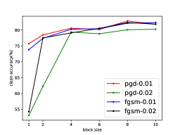
(a) Influence on clean accuracy

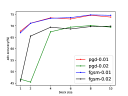
(b) Influence on adversarial accuracy

Figure 1: The effect of block size on the accuracy. In the figure, we show the clean accuracy and the adversarial accuracy of the mean classifier under PGD and FGSM attack with $\epsilon=0.01$ and $\epsilon=0.02$. The block size is choosen from $\{1,2,4,6,8,10\}$. (a) The influence on the clean accuracy; (b) The influence on the adversarial accuracy.

In this section, we conduct several experiments to support our theory. We emphasize that we are not proposing a method to try to get better robustness on the downstream tasks, we do the experiments to verify our two claims from our theoretical results: (1) As shown in Remark 11, using the blocks may improve the robust performance; (2) As shown in Remark 28, using the norms of the layers of the neural networks as the regularizer may help improve the robust performance.

Data sets. We use two data sets (Krizhevsky and Hinton, 2009) in our experiments: (1) the CIFAR-10 data set and (2) the CIFAR-100 data set. CIFAR-10 contains 50000/10000 train/test images with size $32\times 32$, which are categorized into 10 classes. CIFAR-100 contains 50000/10000 train/test images with size $32\times 32$, which are categorized into 100 classes.

Model. We use a neural network with two convolutional layers and one fully connected layer. Following He et al. (2020), we use the Stochastic Gradient Descent (SGD) optimizer with momentum $0.9$ but set the weight decay to be $5\times 10^{-4}$ and the learning rate to be $0.001$.

Evaluation of robustness. For representation $f$, we first calculate $\widehat{u}_{c}=\frac{1}{n_{c}}\sum_{i=1}^{n_{c}}f(x_{i})$ to estimate the $c$-th row of the mean classifier, where $x_{1},\dots,x_{n_{c}}$ are the data points with label $c$ in our training set. Denote $\widehat{W}^{\mu}$ as the estimator of $W$, we use the robustness of the classifier $\widehat{W}^{\mu}f$ as an evaluation of the robustness of $f$ on the downstream task.

We show the results for CIFAR-10 here; the results for CIFAR-100 can be found in the Appendix B.

6.1 Improvement from the regularizer

Inspired by our bound (13) in Theorem 24 and Theorem 8, the adversarial supervised risk can be upper bounded by the sum of the adversarial unsupervised loss and $AG_{M}$, which is related to the maximal Frobenius-norm of the network layers. We choose to simultaneously optimize the contrastive upstream pre-train risk and the Frobenius norm of the parameters of the model. We set the norm of the parameters for the layers as a regularizer and test the performance of the mean classifier; here, $W^{\mu}$ is calculated by averaging all features of the training data set as done in Nozawa et al. (2020). We use a hyper-parameter $\lambda$ to balance the trade-off of the the contrastive upstream pre-train risk and the Frobenius norm of the parameters of the model. We choose to minimize the following regularized empirical risk:

$$L(f)=\widehat{\widetilde{L}}_{sun}(f)+\lambda N(f)$$ (14)

where $N(f)$ is a regularizer that constrains the Frobenius norm of the parameters of the model $f$, here we choose $N(f)=\sum_{l=1}^{d}{\left|\kern-1.07639pt\left|\kern-1.07639pt\left|W_{l}\right|\kern-1.07639pt\right|\kern-1.07639pt\right|}_{F}$ where ${\left|\kern-1.07639pt\left|\kern-1.07639pt\left|W_{l}\right|\kern-1.07639pt\right|\kern-1.07639pt\right|}_{F}$ is the Frobenius norm of the parameters for the $l$-th layer of $f$ and:

$$\widehat{\widetilde{L}}_{sun}(f)\!\!=\!\!\frac{1}{M}\sum_{j=1}^{M}\!\underset{x_{j}^{\prime}\in\mathcal{U}(x_{j})}{\max}\ell(\!\{f(x_{j}^{\prime})^{T}\!(f(x_{j}^{+})\!-\!f(x_{ji}^{-}))\}_{i=1}^{k}).$$

More details about our algorithm are in Algorithm 1.

Input : The training data set $\mathcal{S}=\left\{(x_{j},x_{j}^{+},x_{j1}^{-},\dots,x_{jk}^{-})\right\}_{j=1}^{M}$ sampled from $\mathcal{D}_{sim}\times\mathcal{D}_{neg}^{k}$; the hyper-parameter $\lambda$ in (14); the adversarial perturbation $\mathcal{U}$; learning rate $\alpha$; the total iteration number $T$;

1 initialize $\theta^{0}$ to be randomized parameters;

2 $t\leftarrow 0$;

3 while $t<T$ do

4       randomly sample a batch of data with size $N$: $\mathcal{B}\subseteq\mathcal{S}$ ;

5       $\widetilde{\mathcal{B}}\leftarrow\emptyset$;

6       for $(x,x^{+},x_{1}^{-},\dots,x_{k}^{-})$ in $\mathcal{B}$ do

7             calculate adversarial example $\tilde{x}\in\underset{x^{\prime}\in\mathcal{U}(x)}{\arg\sup}\ \ell\left(\left\{f_{\theta^{t}}(x^{\prime})^{T}\left(f_{\theta^{t}}(x^{+})-f_{\theta^{t}}(x_{i}^{-})\right)\right\}_{i=1}^{k}\right)$;

8             $\widetilde{\mathcal{B}}\leftarrow\widetilde{\mathcal{B}}\cup\{(\tilde{x},x^{+},x_{1}^{-},\dots,x_{k}^{-})\}$;

9            

10       end for

11      $L(f_{\theta^{t}})=\frac{1}{N}\sum_{(\tilde{x},x^{+},x_{1}^{-},\dots,x_{k}^{-})\in\widetilde{\mathcal{B}}}\ell\left(\left\{f_{\theta^{t}}(\tilde{x})^{T}\left(f_{\theta^{t}}(x^{+})-f_{\theta^{t}}(x_{i}^{-})\right)\right\}_{i=1}^{k}\right)+\lambda N(f_{\theta^{t}})$;

12       $\theta^{t+1}\leftarrow\theta^{t}-\alpha\nabla_{\theta^{t}}L(f_{\theta^{t}})$;

13       $t\leftarrow t+1$;

14      

15 end while

Output : The feature extractor $f_{\theta^{T}}\in\mathcal{F}$ that tries to minimize (14);

Algorithm 1 The AERM algorithm for adversarial contrastive learning

The results are shown in Table 1. From Table 1, we can see that the $F$-norm regularizer can improve the adversarial accuracy (the prediction performance of a model on adversarial examples generated by attacker) of the mean classifier, which is in line with our Theorem 24.

6.2 Effect of block size

To verify Theorem 10, we analyze the effect of block size on the adversarial accuracy of the mean classifier. Figure 1 presents the results for clean accuracy and adversarial accuracy, respectively. From Figure 1, we can see that a larger block size will yield better adversarial accuracy. The results are consistent with Theorem 10: as the block size grows, Theorem 10 shows that we are optimizing a tighter bound, which leads to better performance as shown in Figure 1.

7 Conclusion

This paper studies the generalization performance of adversarial contrastive learning. We first extend the contrastive learning framework to the adversarial case, then we upper bound the average adversarial risk of the downstream tasks with the adversarial unsupervised risk of the upstream task and an adversarial Rademacher complexity term. Furthermore, we provide the upper bound of the adversarial Rademacher complexity for linear models and multi-layer neural networks. Finally, we conduct several experiments and the experimental results are consistent with our theory.

Acknowledgments and Disclosure of Funding

This work is supported by the National Natural Science Foundation of China under Grant 61976161.

Appendix A Proofs

In this section, we display the proofs of our theorems, lemmas and corollaries. For reading convenience, we will restate the theorem before proving.

A.1 Proof of Theorem 8

In the below, we present some useful lemmas that will be used in the proofs of our main theorems.

Lemma 29

For any $f\in\mathcal{F}$, we have:

$$\widetilde{L}_{sup}(f) \leq\widetilde{L}_{sup}^{\mu}(f)\leq\frac{1}{1-\tau}(\widetilde{L}_{un}(f)-\tau\ell(0))\leq\frac{1}{1-\tau}(\widetilde{L}_{sun}(f)-\tau\ell(0)).$$ (A.1)

Remark 30

$\widehat{\widetilde{L}}_{sun}(f)$ denotes the empirical $\widetilde{L}_{sun}(f)$ and $\widehat{f}\in\underset{f\in\mathcal{F}}{\arg\min}\ \widehat{\widetilde{L}}_{sun}(f)$. Applying Lemma 29 to $\widehat{f}$ shows that, if we can train a robust feature extractor with low surrogate adversarial unsupervised risk, we can obtain a robust classifier with low adversarial supervised risk on the downstream task.

Lemma 31

Let $\ell:\mathbb{R}^{k}\xrightarrow[]{}\mathbb{R}$ be bounded by $B$. Then, for any $\delta\in(0,1)$, with a probability of at least $1-\delta$ over the choice of the training set $\mathcal{S}=\{(x_{j},x_{j}^{+},x_{j1}^{-},\dots,x_{jk}^{-})\}_{j=1}^{M}=\{z_{j}\}_{j=1}^{M}$, for any $f\in\mathcal{F}$:

$$\widetilde{L}_{sun}(\widehat{f})\leq\widetilde{L}_{sun}(f)+AG_{M},$$

where $AG_{M}=O(\frac{\mathcal{R}_{\mathcal{S}}(\mathcal{G})}{M}+B\sqrt{\frac{log\frac{1}{\delta}}{M}}),\ \ \mathcal{R}_{\mathcal{S}}(\mathcal{G})\coloneqq\underset{\bm{\sigma}\sim\{\pm 1\}^{M}}{\mathbb{E}}\left[\underset{f\in\mathcal{F}}{\sup}\left<\bm{\sigma},(g_{f})_{|\mathcal{S}}\right>\right],$ and $\mathcal{G}\coloneqq\{g_{f}(x,x^{+},x_{1}^{-},\dots,x_{k}^{-})=\underset{x^{\prime}\in\mathcal{U}(x)}{\sup}\ell\left(\{f(x^{\prime})^{T}(f(x^{+})-f(x_{i}^{-}))\}_{i=1}^{k}\right)|f\in\mathcal{F}\},$ where $\bm{\sigma}$ is an $M$-dimensional Rademacher random vector with i.i.d. entries and $(g_{f})_{|\mathcal{S}}=\left(g_{f}(z_{1}),\dots,g_{f}(z_{M})\right)$.

Proof [Proof of Lemma 29] By the definition of $\widetilde{L}_{sup}(\mathcal{T},f)$, i.e., (3), it’s obvious that $\widetilde{L}_{sup}(f)\leq\widetilde{L}_{sup}^{\mu}(f)$, so we only need to prove the second part of (A.1). From definition (2), we have, $\forall{f\in\mathcal{F}}$:

$$\widetilde{L}_{un}(f) =\underset{c^{+},c^{-}\sim\rho^{2}}{\mathbb{E}}\left\{\underset{x\sim\mathcal{D}_{c^{+}}}{\mathbb{E}}\left[\underset{x^{\prime}\in\mathcal{U}(x)}{\sup}\left(\underset{x^{-}\sim\mathcal{D}_{c^{-}}}{\underset{x^{+}\sim\mathcal{D}_{c^{+}}}{\mathbb{E}}}\left(\ell\left(f(x^{\prime})^{T}\left(f(x^{+})-f(x^{-})\right)\right)\right)\right)\right]\right\}$$ (A.2)

$$\overset{(\text{i})}{\geq}\underset{c^{+},c^{-}\sim\rho^{2}}{\mathbb{E}}\left\{\underset{x\sim\mathcal{D}_{c^{+}}}{\mathbb{E}}\left[\underset{x^{\prime}\in\mathcal{U}(x)}{\sup}\ell\left(f(x^{\prime})^{T}(\mu_{c^{+}}-\mu_{c^{-}})\right)\right]\right\}$$

$$\overset{(\text{ii})}{=}(1-\tau)\underset{c^{+},c^{-}\sim\rho^{2}}{\mathbb{E}}\left\{\underset{x\sim\mathcal{D}_{c^{+}}}{\mathbb{E}}\left[\underset{x^{\prime}\in\mathcal{U}(x)}{\sup}\ell\left(f(x^{\prime})^{T}(\mu_{c^{+}}-\mu_{c^{-}})\right)\right]\Bigg{|}c^{+}\neq c^{-}\right\}+\tau\ell(0),$$

where $(\text{i})$ comes from the convexity of $\ell$ and Jensen’s Inequality, and $(\text{ii})$ comes from the property of conditional expectations. Then we have:

$$\underset{c^{+},c^{-}\sim\rho^{2}}{\mathbb{E}}\left\{\underset{x\sim\mathcal{D}_{c^{+}}}{\mathbb{E}}\left[\underset{x^{\prime}\in\mathcal{U}(x)}{\sup}\ell\left(f(x^{\prime})^{T}(\mu_{c^{+}}-\mu_{c^{-}})\right)\right]\Bigg{|}c^{+}\neq c^{-}\right\}$$ (A.3)

$$\overset{(\text{i})}{=}\underset{c^{+},c^{-}\sim\rho^{2}}{\mathbb{E}}\Bigg{\{}D_{\mathcal{T}}(c^{+})\underset{x\sim\mathcal{D}_{c^{+}}}{\mathbb{E}}\left[\underset{x^{\prime}\in\mathcal{U}(x)}{\sup}\ell\left(f(x^{\prime})^{T}(\mu_{c^{+}}-\mu_{c^{-}})\right)\right]$$

$$\ \ \ \ \ \ \ \ \ \ \ \ +D_{\mathcal{T}}(c^{-})\underset{x\sim\mathcal{D}_{c^{-}}}{\mathbb{E}}\left[\underset{x^{\prime}\in\mathcal{U}(x)}{\sup}\ell\left(f(x^{\prime})^{T}(\mu_{c^{-}}-\mu_{c^{+}})\right)\right]\Bigg{|}c^{+}\neq c^{-}\Bigg{\}}$$

$$\overset{(\text{ii})}{=}\underset{c^{+},c^{-}\sim\rho^{2}}{\mathbb{E}}\Bigg{\{}D_{\mathcal{T}}(c^{+})\underset{x\sim\mathcal{D}_{c^{+}}}{\mathbb{E}}\left[\underset{x^{\prime}\in\mathcal{U}(x)}{\sup}\ell\left(g(x^{\prime})_{c^{+}}-g(x^{\prime})_{c^{-}}\right)\right]$$

$$\ \ \ \ \ \ \ \ \ \ \ \ +D_{\mathcal{T}}(c^{-})\underset{x\sim\mathcal{D}_{c^{-}}}{\mathbb{E}}\left[\underset{x^{\prime}\in\mathcal{U}(x)}{\sup}\ell\left(g(x^{\prime})_{c^{-}}-g(x^{\prime})_{c^{+}}\right)\right]\Bigg{|}c^{+}\neq c^{-}\Bigg{\}},$$

where $\mathcal{T}=\{c^{+},c^{-}\}$, $g(x)=\begin{bmatrix}\mu_{c^{+}}^{T}f(x)\\ \mu_{c^{-}}^{T}f(x)\end{bmatrix}=W^{\mu}f(x)$ and $(\text{i})$ comes from the symmetry of $c^{+},c^{-}$; $(\text{ii})$ is directly from some linear algebras. From (A.3) we know that:

$$\underset{c^{+},c^{-}\sim\rho^{2}}{\mathbb{E}}\left\{\underset{x\sim\mathcal{D}_{c^{+}}}{\mathbb{E}}\left[\underset{x^{\prime}\in\mathcal{U}(x)}{\sup}\ell\left(f(x^{\prime})^{T}(\mu_{c^{+}}-\mu_{c^{-}})\right)\right]\Bigg{|}c^{+}\neq c^{-}\right\}$$ (A.4)

$$\overset{(\text{i})}{=}\underset{c^{+},c^{-}\sim\rho^{2}}{\mathbb{E}}\left\{\underset{c\sim\mathcal{D}_{\mathcal{T}}}{\mathbb{E}}\underset{x\sim\mathcal{D}_{c}}{\mathbb{E}}\left[\underset{x^{\prime}\in\mathcal{U}(x)}{\sup}\ell\left(\left\{g(x^{\prime})_{c}-g(x^{\prime})_{c^{\prime}}\right\}_{c^{\prime}\neq c}\right)\right]\Bigg{|}c^{+}\neq c^{-}\right\}$$

$$\overset{(\text{ii})}{=}\underset{c^{+},c^{-}\sim\rho^{2}}{\mathbb{E}}\left[\widetilde{L}_{sup}\left(\left\{c^{+},c^{-}\right\},W^{\mu}f\right)\Bigg{|}c^{+}\neq c^{-}\right]$$

$$\overset{(\text{iii})}{=}\underset{c^{+},c^{-}\sim\rho^{2}}{\mathbb{E}}\left[\widetilde{L}_{sup}^{\mu}\left(\left\{c^{+},c^{-}\right\},f\right)\Bigg{|}c^{+}\neq c^{-}\right]\overset{(\text{iv})}{=}\widetilde{L}_{sup}^{\mu}(f),$$

where $(\text{i})$ is due to the tower property of expectation;$(\text{ii})$ is obvious by the definition of $\widetilde{L}_{sup}(\mathcal{T},g)$; $(\text{iii})$ comes from the definition of $\widetilde{L}_{sup}^{\mu}(\mathcal{T},f)$ and $(\text{iv})$ is from the definition of $\widetilde{L}_{sup}^{\mu}(f)$. Combine (A.2) with (A.4), we conclude that:

$$\widetilde{L}_{un}(f)\geq(1-\tau)\widetilde{L}_{sup}^{\mu}(f)+\tau\ell(0),\forall{f\in\mathcal{F}}.$$

So we have:

$$(1-\tau)\widetilde{L}_{sup}(f)+\tau\ell(0)\leq(1-\tau)\widetilde{L}_{sup}^{\mu}(f)+\tau\ell(0)\leq\widetilde{L}_{un}(f),\forall{f\in\mathcal{F}}.$$ (A.5)

Rearranging (A.5) yields (A.1).  

Proof [Proof of Lemma 31] Denote $(x,x^{+},x_{1}^{-},\cdots,x_{k}^{-})$ by $z$, then by the Theorem 3.3 in Mohri et al. (2012), we have: With probability at least $1-\frac{\delta}{2}$ over the choice of the training set $\mathcal{S}$,

$$\underset{z}{\mathbb{E}}\left[\frac{1}{B}g_{f}(z)\right]\leq\frac{1}{M}\sum_{i=1}^{M}\frac{1}{B}g_{f}(z_{i})+\frac{2}{M}\mathcal{R}_{\mathcal{S}}(\frac{\mathcal{G}}{B})+3\sqrt{\frac{log\frac{4}{\delta}}{M}},$$

which is equivalent to:

$$\widetilde{L}_{sun}(f)\leq\widehat{\widetilde{L}}_{sun}(f)+\frac{2}{M}\mathcal{R}_{\mathcal{S}}(\mathcal{G})+3B\sqrt{\frac{log\frac{4}{\delta}}{M}},\forall{f\in\mathcal{F}}.$$ (A.6)

Let $f^{*}=\underset{f\in\mathcal{F}}{\arg\min}\ \widetilde{L}_{sun}(f)$, since $\underset{\mathcal{S}}{\mathbb{E}}\left[\widehat{\widetilde{L}}_{sun}(f)\right]=\widetilde{L}_{sun}(f)$ and $\ell$ is bounded by $B$, Hoeffding’s inequality tells us that: $\forall{f\in\mathcal{F}}$, $\forall{t\in\mathbb{R}}$:

$$\mathbb{P}\left[\widehat{\widetilde{L}}_{sun}(f)-\widetilde{L}_{sun}(f)\geq t\right]\leq e^{-\frac{2Mt^{2}}{B^{2}}}.$$

Set $t=B\sqrt{\frac{log\frac{2}{\delta}}{2M}}$, we have: $\forall{f\in\mathcal{F}}$, with probability at least $1-\frac{\delta}{2}$,

$$\widehat{\widetilde{L}}_{sun}(f)-\widetilde{L}_{sun}(f)\leq B\sqrt{\frac{log\frac{2}{\delta}}{2M}}.$$ (A.7)

Combine (A.6) with (A.7), the union bound tells us that: $\forall{f\in\mathcal{F}}$, with probability at least $1-\delta$ over the choice of the training set $\mathcal{S}$,

$$\widetilde{L}_{sun}(\widehat{f}) \overset{(\text{i})}{\leq}\widehat{\widetilde{L}}_{sun}(\widehat{f})+O\left(\frac{\mathcal{R}_{\mathcal{S}}(\mathcal{G})}{M}+B\sqrt{\frac{log\frac{1}{\delta}}{M}}\right)\overset{(\text{ii})}{\leq}\widehat{\widetilde{L}}_{sun}(f^{*})+O\left(\frac{\mathcal{R}_{\mathcal{S}}(\mathcal{G})}{M}+B\sqrt{\frac{log\frac{1}{\delta}}{M}}\right)$$

$$\overset{(\text{iii})}{\leq}\widetilde{L}_{sun}(f^{*})+O\left(\frac{\mathcal{R}_{\mathcal{S}}(\mathcal{G})}{M}+B\sqrt{\frac{log\frac{1}{\delta}}{M}}\right)\overset{(\text{iv})}{\leq}\widetilde{L}_{sun}(f)+O\left(\frac{\mathcal{R}_{\mathcal{S}}(\mathcal{G})}{M}+B\sqrt{\frac{log\frac{1}{\delta}}{M}}\right),$$

where $(\text{i})$ comes from (A.6);$(\text{ii})$ is directly from the fact that $\widehat{\widetilde{L}}_{sun}(\widehat{f})\leq\widehat{\widetilde{L}}_{sun}(f^{*})$, which is from the definition of $\widehat{f}$;$(\text{iii})$ is a result of (A.7) and $(\text{iv})$ is obvious by the definition of $f^{*}$.  

Theorem 8

Let $\ell:\mathbb{R}^{k}\xrightarrow[]{}\mathbb{R}$ be bounded by $B$. Then, for any $\delta\in(0,1)$,with a probability of at least $1-\delta$ over the choice of the training set $\mathcal{S}=\{(x_{j},x_{j}^{+},x_{j}^{-})\}_{j=1}^{M}$, for any $f\in\mathcal{F}$:

$$\widetilde{L}_{sup}(\widehat{f})\leq\widetilde{L}_{sup}^{\mu}(\widehat{f})\leq\frac{1}{1-\tau}(\widetilde{L}_{sun}(f)-\tau\ell(0))+\frac{1}{1-\tau}AG_{M}.$$

Proof  From Lemma 29 we know that:

$$\widetilde{L}_{sup}(\widehat{f})\leq\widetilde{L}_{sup}^{\mu}(\widehat{f})\leq\frac{1}{1-\tau}(\widetilde{L}_{un}(\widehat{f})-\tau\ell(0))\leq\frac{1}{1-\tau}(\widetilde{L}_{sun}(\widehat{f})-\tau\ell(0)),$$

Then Lemma 31 directly yields the result we need.  

A.2 Proof of Theorem 10

Theorem 10

For any $f\in\mathcal{F}$, we have:

$$\widetilde{L}_{sup}(f) \leq\frac{1}{1-\tau}\left(\widetilde{L}_{sun}^{block}(f)-\tau\ell(0)\right)\leq\frac{1}{1-\tau}\left(\widetilde{L}_{sun}(f)-\tau\ell(0)\right).$$

Proof  By the convexity of $\ell$ and Jensen’s inequality, we have: $\forall{x^{\prime},x_{i}^{+},x_{i}^{-}}$:

$$\ell\left(f(x^{\prime})^{T}\left(\frac{\sum_{i=1}^{b}f(x_{i}^{+})}{b}-\frac{\sum_{i=1}^{b}f(x_{i}^{-})}{b}\right)\right) =\ell\left(\frac{1}{b}\sum_{i=1}^{b}f(x^{\prime})^{T}\left(f(x_{i}^{+})-f(x_{i}^{-})\right)\right)$$

$$\leq\frac{1}{b}\sum_{i=1}^{b}\ell\left(f(x^{\prime})^{T}\left(f(x_{i}^{+})-f(x_{i}^{-})\right)\right).$$

Take maximization about $x^{\prime}$ both sides, we have:

$$\underset{x^{\prime}\in\mathcal{U}(x)}{\sup}\!\ell\!\left(\!f(x^{\prime})^{T}\!\!\left(\frac{\sum_{i=1}^{b}f(x_{i}^{+}\!)}{b}\!-\!\frac{\sum_{i=1}^{b}f(x_{i}^{-}\!)}{b}\right)\!\!\!\right) \!\leq\!\frac{1}{b}\underset{x^{\prime}\in\mathcal{U}(x)}{\sup}\!\!\left[\sum_{i=1}^{b}\!\ell\!\left(f(x^{\prime})^{T}\!\!\left(f(x_{i}^{+}\!)\!-\!f(x_{i}^{-})\right)\right)\!\right]$$

$$\!\leq\!\frac{1}{b}\sum_{i=1}^{b}\!\left[\underset{x^{\prime}\in\mathcal{U}(x)}{\sup}\!\ell\!\left(f(x^{\prime})^{T}\!\!\left(f(x_{i}^{+}\!)\!-\!f(x_{i}^{-}\!)\!\right)\!\right)\!\right].$$

Taking expectations both sides yields:

$$\widetilde{L}_{sun}^{block}(f) =\underset{x,x_{i}^{+},x_{i}^{-}}{\mathbb{E}}\left[\underset{x^{\prime}\in\mathcal{U}(x)}{\sup}\ell\left(f(x^{\prime})^{T}\left(\frac{\sum_{i=1}^{b}f(x_{i}^{+})}{b}-\frac{\sum_{i=1}^{b}f(x_{i}^{-})}{b}\right)\right)\right]$$

$$\leq\underset{x,x_{i}^{+},x_{i}^{-}}{\mathbb{E}}\left\{\frac{1}{b}\sum_{i=1}^{b}\left[\underset{x^{\prime}\in\mathcal{U}(x)}{\sup}\ell\left(f(x^{\prime})^{T}\left(f(x_{i}^{+})-f(x_{i}^{-})\right)\right)\right]\right\}$$

$$=\underset{x,x^{+},x^{-}}{\mathbb{E}}\left[\underset{x^{\prime}\in\mathcal{U}(x)}{\sup}\ell\left(f(x^{\prime})^{T}\left(f(x^{+})-f(x^{-})\right)\right)\right]=\widetilde{L}_{sun}(f),$$

which proves the second inequality. For the first inequality, we have, $\forall{f\in\mathcal{F}}$:

$$\widetilde{L}_{sun}^{block}(f) =\underset{c^{+},c^{-}\sim\rho^{2}}{\mathbb{E}}\left\{\underset{x_{i}^{-}\sim\mathcal{D}_{c^{-}}^{b}}{\underset{x,x_{i}^{+}\sim\mathcal{D}_{c^{+}}^{b+1}}{E}}\left[\underset{x^{\prime}\in\mathcal{U}(x)}{\sup}\ell\left(f(x^{\prime})^{T}\left(\frac{\sum_{i=1}^{b}f(x_{i}^{+})}{b}-\frac{\sum_{i=1}^{b}f(x_{i}^{-})}{b}\right)\right)\right]\right\}$$

$$\overset{(\text{i})}{\geq}\!\!\underset{c^{+},c^{-}\sim\rho^{2}}{\mathbb{E}}\!\!\!\left\{\!\underset{x\sim\mathcal{D}_{c^{+}}}{\mathbb{E}}\!\!\left\{\underset{x^{\prime}\in\mathcal{U}(x)}{\sup}\underset{x_{i}^{-}\sim\mathcal{D}_{c^{-}}^{b}}{\underset{x_{i}^{+}\sim\mathcal{D}_{c^{+}}^{b}}{E}}\!\!\left[\ell\!\left(f(x^{\prime})^{T}\!\!\left(\frac{\sum_{i=1}^{b}f(x_{i}^{+})}{b}\!-\!\frac{\sum_{i=1}^{b}f(x_{i}^{-})}{b}\right)\right)\right]\right\}\right\}$$

$$\overset{(\text{ii})}{\geq}\!\!\underset{c^{+},c^{-}\sim\rho^{2}}{\mathbb{E}}\!\!\!\left\{\!\underset{x\sim\mathcal{D}_{c^{+}}}{\mathbb{E}}\!\!\left\{\underset{x^{\prime}\in\mathcal{U}(x)}{\sup}\ell\!\!\left[\underset{x_{i}^{-}\sim\mathcal{D}_{c^{-}}^{b}}{\underset{x_{i}^{+}\sim\mathcal{D}_{c^{+}}^{b}}{E}}\!\!\!\left(f(x^{\prime})^{T}\!\!\left(\frac{\sum_{i=1}^{b}f(x_{i}^{+})}{b}\!-\!\frac{\sum_{i=1}^{b}f(x_{i}^{-})}{b}\right)\right)\right]\right\}\right\}$$

$$\overset{(\text{iii})}{=}\underset{c^{+},c^{-}\sim\rho^{2}}{\mathbb{E}}\left\{\underset{x\sim\mathcal{D}_{c^{+}}}{\mathbb{E}}\left[\underset{x^{\prime}\in\mathcal{U}(x)}{\sup}\ell\left(f(x^{\prime})^{T}(\mu_{c^{+}}-\mu_{c^{-}})\right)\right]\right\}\overset{(\text{iv})}{=}(1-\tau)\widetilde{L}_{sup}^{\mu}(f)+\tau\ell(0),$$

where $(\text{i})$ and $(\text{ii})$ are directs result of Jensen’s Inequality and convexity of maximization function and $\ell$; $(\text{iii})$ is from the linearity of expectation and the last equality follows the same argumentation as in (A.4), which proves the Theorem.  

A.3 Proof of (5)

Proof  For any $f\in\mathcal{F}$, we have:

$$\widetilde{\mathcal{L}}_{sup}(f) =\!\!\underset{\mathcal{T}\sim\mathcal{D}}{\mathbb{E}}\left[\widetilde{L}_{sup}(\mathcal{T},f)\right]\!\overset{(\text{i})}{=}\!p\!\ \underset{\mathcal{T}\sim\mathcal{D}}{\mathbb{E}}\left[\widetilde{L}_{sup}(\mathcal{T},f)\Big{|}E_{distinct}\right]\!+\!(1\!-\!p)\underset{\mathcal{T}\sim\mathcal{D}}{\mathbb{E}}\left[\widetilde{L}_{sup}(\mathcal{T},f)\Big{|}\bar{E}_{distinct}\right]$$

$$\geq p\ \underset{\mathcal{T}\sim\mathcal{D}}{\mathbb{E}}\left[\widetilde{L}_{sup}(\mathcal{T},f)\Big{|}E_{distinct}\right]\overset{(\text{ii})}{=}p\ \widetilde{L}_{sup}(f),$$

where $E_{distinct}$ is the event that $\{c^{+},c_{1}^{-},\dots,c_{k}^{-}\}$ is distinct and $p=\underset{(c^{+},c_{1}^{-},\dots,c_{k}^{-})\sim\mathcal{D}}{P}[E_{distinct}]$ and $(\text{i})$ is from the property of conditional expectation and $(\text{ii})$ comes from the definition of $\widetilde{L}_{sup}(f)$.  

A.4 Proof of Proposition 15

Proposition 15

The hinge loss and the logistic loss satisfy Assumption 14.

Proof  Since $I_{1}$ and $I_{2}$ are symmetric, We only need to prove (6). For the Hinge Loss:

$$\ell\left(\{v_{i}\}_{i\in I_{1}}\right) =\max\left\{0,1+\underset{i\in I_{1}}{\max}\{-v_{i}\}\right\} \overset{(\text{i})}{\leq}\max\left\{0,1+\underset{i\in[d]}{\max}\{-v_{i}\}\right\}=\ell\left(\{v_{i}\}_{i\in[d]}\right),$$

where $(\text{i})$ is from the fact that $I_{1}\subseteq[d]$, so the first inequality is proved, for the second one:

$$\ell\left(\{v_{i}\}_{i\in[d]}\right) =\max\left\{0,1+\underset{i\in[d]}{\max}\{-v_{i}\}\right\}=\max\left\{0,1+\underset{i\in I_{1}\cup I_{2}}{\max}\{-v_{i}\}\right\},$$

where the last equality is directly from the definition of $I_{1}$ and $I_{2}$.

1. if   $1+\underset{i\in I_{1}\cup I_{2}}{\max}\{-v_{i}\}\leq 0$, then $\ell\left(\{v_{i}\}_{i\in I_{1}\cup I_{2}}\right)=0$, since Hinge Loss is non-negative, we have:

   $$\ell\left(\{v_{i}\}_{i\in I_{1}\cup I_{2}}\right)=0+0\leq\ell\left(\{v_{i}\}_{i\in I_{1}}\right)+\ell\left(\{v_{i}\}_{i\in I_{2}}\right).$$

2. if   $1+\underset{i\in I_{1}\cup I_{2}}{\max}\{-v_{i}\}>0$

   1. if  $1+\underset{i\in I_{1}}{\max}\{-v_{i}\}\leq 0$, then $\ell\left(\{v_{i}\}_{i\in I_{1}}\right)=\max\left\{0,1+\underset{i\in I_{1}}{\max}\{-v_{i}\}\right\}=0$. So we have:

      $$\ell\left(\{v_{i}\}_{i\in I_{1}\cup I_{2}}\right) =\max\left\{0,1+\underset{i\in I_{1}\cup I_{2}}{\max}\{-v_{i}\}\right\}=\max\left\{0,1+\underset{i\in I_{2}}{\max}\{-v_{i}\}\right\}$$

      $$=0+\ell\left(\{v_{i}\}_{i\in I_{2}}\right)=\ell\left(\{v_{i}\}_{i\in I_{1}}\right)+\ell\left(\{v_{i}\}_{i\in I_{2}}\right).$$

   2. if  $1+\underset{i\in I_{2}}{\max}\{-v_{i}\}\leq 0$, by the same discussion of (a), we have:

      $$\ell\left(\{v_{i}\}_{i\in I_{1}\cup I_{2}}\right)\leq\ell\left(\{v_{i}\}_{i\in I_{1}}\right)+\ell\left(\{v_{i}\}_{i\in I_{2}}\right).$$

   3. if  $1+\underset{i\in I_{1}}{\max}\{-v_{i}\}>0$   and   $1+\underset{i\in I_{2}}{\max}\{-v_{i}\}>0$,

      $$\ell\left(\{v_{i}\}_{i\in I_{1}\cup I_{2}}\right) =\!\max\!\left\{0,1\!+\!\!\!\underset{i\in I_{1}\cup I_{2}}{\max}\{-v_{i}\}\!\right\}\!\leq\!\max\!\left\{0,1\!+\!\!\underset{i\in I_{1}}{\max}\{-v_{i}\}\!+\!1\!+\!\!\underset{i\in I_{2}}{\max}\{-v_{i}\}\right\}$$

      $$\leq\max\left\{0,1+\underset{i\in I_{1}}{\max}\{-v_{i}\}\right\}+\max\left\{0,1+\underset{i\in I_{2}}{\max}\{-v_{i}\}\right\}$$

      $$=\ell\left(\{v_{i}\}_{i\in I_{1}}\right)+\ell\left(\{v_{i}\}_{i\in I_{2}}\right).$$

So the second inequality is proved. For the Logistic Loss:

$$\ell\left(\{v_{i}\}_{i\in I_{1}}\right) =log_{2}\left(1+\sum_{i\in I_{1}}e^{-v_{i}}\right)\leq log_{2}\left(1+\sum_{i\in[d]}e^{-v_{i}}\right)=\ell\left(\{v_{i}\}_{i\in[d]}\right).$$

So the first inequality is proved. For the second one:

$$\ell\left(\{v_{i}\}_{i\in I_{1}\cup I_{2}}\right) =log_{2}\left(1+\sum_{i\in I_{1}\cup I_{2}}e^{-v_{i}}\right)\leq log_{2}\left(1+\sum_{i\in I_{1}}e^{-v_{i}}+\sum_{i\in I_{2}}e^{-v_{i}}\right)$$

$$\leq log_{2}\left(1+\sum_{i\in I_{1}}e^{-v_{i}}+\sum_{i\in I_{2}}e^{-v_{i}}+\left(\sum_{i\in I_{1}}e^{-v_{i}}\right)\left(\sum_{i\in I_{2}}e^{-v_{i}}\right)\right)$$

$$=log_{2}\left[\left(1+\sum_{i\in I_{1}}e^{-v_{i}}\right)\left(1+\sum_{i\in I_{2}}e^{-v_{i}}\right)\right]$$

$$=log_{2}\left(1+\sum_{i\in I_{1}}e^{-v_{i}}\right)+log_{2}\left(1+\sum_{i\in I_{2}}e^{-v_{i}}\right)=\ell\left(\{v_{i}\}_{i\in I_{1}}\right)+\ell\left(\{v_{i}\}_{i\in I_{2}}\right),$$

which proves the second inequality.  

A.5 Proof of Theorem 32

We here introduce some further notations, which will be used in our main results. For a tuple $(c^{+},c_{1}^{-},\dots,c_{k}^{-})$, we define $I^{+}\coloneqq\{i\in[k]|c_{i}^{-}=c^{+}\}$ and $Q$ as the set of distinct classes in $(c^{+},c_{1}^{-},\dots,c_{k}^{-})$. We define $p_{\max}(\mathcal{T})\coloneqq\max_{c}\mathcal{D}_{\mathcal{T}}(c)$, $\tau_{k}\coloneqq\underset{c^{+},c_{i}^{-}\sim\rho^{k+1}}{\mathbb{P}}[I^{+}\neq\emptyset]$, while $\ell_{N}(\vec{0})$ is defined as the loss of the $N$-dimensional zero vector. Let $\mathcal{T}$ be a task sample from distribution $\mathcal{D}$ and $\rho^{+}(\mathcal{T})$ be a distribution of $c^{+}$ when $(c^{+},c_{1}^{-},\dots,c_{k}^{-})$ are sampled from $\rho^{k+1}$ conditioned on $Q=\mathcal{T}$ and $I^{+}=\emptyset$ and $\rho_{\min}^{+}(\mathcal{T})\coloneqq\underset{c\in\mathcal{T}}{\min}\ \rho^{+}(\mathcal{T})(c)$.

Theorem 32

Assume that $\ell$ satisfies Assumption 14. With a probability of at least $1-\delta$ over the choice of the training set $\mathcal{S}$, for any $f\in\mathcal{F}$, we have:

$$\underset{\mathcal{T}\sim\mathcal{D}}{\mathbb{E}}\!\!\left[\frac{\rho_{\min}^{+}(\mathcal{T})}{p_{\max}(\mathcal{T})}\widetilde{L}_{sup}(\mathcal{T},\widehat{f})\right]\!\!\!\leq\!\!\underset{\mathcal{T}\sim\mathcal{D}}{\mathbb{E}}\!\!\left[\frac{\rho_{\min}^{+}(\mathcal{T})}{p_{\max}(\mathcal{T})}\widetilde{L}_{sup}^{\mu}(\mathcal{T},\widehat{f})\right]$$ (A.8)

$$\leq\frac{1}{1-\tau_{k}}\left(\widetilde{L}_{sun}(f)+AG_{M}\right)-\frac{\tau_{k}}{1-\tau_{k}}\underset{c^{+},c_{i}^{-}\sim\rho^{k+1}}{\mathbb{E}}\left[\ell_{|I^{+}|}(\vec{0})|I^{+}\neq\emptyset\right],$$

where $|I^{+}|$ is the cardinality of set $I^{+}$.

Before proceeding with the proof of Theorem 32, we introduce some useful lemmas.

Lemma 33

For any $\mathcal{T}$ sampled from $\mathcal{D}$, we have: $\rho^{+}(\mathcal{T})(c)\geq\frac{\rho_{\min}^{+}(\mathcal{T})}{p_{\max}(\mathcal{T})}\mathcal{D}_{\mathcal{T}}(c),\forall{c\in\mathcal{T}}.$

Lemma 34

Assume that $f$ satisfies Assumption 14. For any $f\in\mathcal{F}$, we have:

$$(1-\tau_{k})\underset{\mathcal{T}\sim\mathcal{D}}{\mathbb{E}}\left[\frac{\rho_{\min}^{+}(\mathcal{T})}{p_{\max}(\mathcal{T})}\widetilde{L}_{sup}(\mathcal{T},f)\right]\leq(1-\tau_{k})\underset{\mathcal{T}\sim\mathcal{D}}{\mathbb{E}}\left[\frac{\rho_{\min}^{+}(\mathcal{T})}{p_{\max}(\mathcal{T})}\widetilde{L}_{sup}^{\mu}(\mathcal{T},f)\right]$$

$$\leq\widetilde{L}_{sun}(f)-\tau_{k}\underset{c^{+},c_{i}^{-}\sim\rho^{k+1}}{\mathbb{E}}\left[\ell_{|I^{+}|}(\vec{0})|I^{+}\neq\emptyset\right].$$

Proof [Proof of Lemma 33] By the definition of $\rho^{+}(\mathcal{T})$ and $\rho_{\min}^{+}(\mathcal{T})$, we can find that:

$$\forall{c\in\mathcal{T}},\rho_{\min}^{+}(\mathcal{T})\leq\rho^{+}(\mathcal{T})(c).$$

So we have:

$$\forall{c\in\mathcal{T}},\frac{\rho^{+}(\mathcal{T})(c)}{\rho_{\min}^{+}(\mathcal{T})}\geq 1.$$ (A.9)

By the definition of $p_{\max}(\mathcal{T})$, we have:

$$\forall{c\in\mathcal{T}},\frac{\mathcal{D}_{\mathcal{T}}(c)}{p_{\max}(\mathcal{T})}\leq 1.$$ (A.10)

Combine (A.9) and (A.10), we have:

$$\forall{c\in\mathcal{T}},\rho^{+}(\mathcal{T})(c)\geq\frac{\rho_{\min}^{+}(\mathcal{T})}{p_{\max}(\mathcal{T})}\mathcal{D}_{\mathcal{T}}(c).$$

 

Proof [Proof of Lemma 34] By the definition of $\widetilde{L}_{sun}(f)$, we have:

$$\widetilde{L}_{sun}(f) =\underset{x,x^{+}\sim\mathcal{D}_{c^{+}}^{2};x_{i}^{-}\sim\mathcal{D}_{c_{i}^{-}}}{\underset{c^{+},c_{i}^{-}\sim\rho^{k+1}}{\mathbb{E}}}\left[\underset{x^{\prime}\in\mathcal{U}(x)}{\sup}\ell\left(\left\{f(x^{\prime})^{T}\left(f(x^{+})-f(x_{i}^{-})\right)\right\}_{i=1}^{k}\right)\right]$$ (A.11)

$$=\underset{x\sim\mathcal{D}_{c^{+}}}{\underset{c^{+},c_{i}^{-}\sim\rho^{k+1}}{\mathbb{E}}}\left\{\underset{x_{i}^{-}\sim\mathcal{D}_{c_{i}^{-}}}{\underset{x^{+}\sim\mathcal{D}_{c^{+}}}{\mathbb{E}}}\left[\underset{x^{\prime}\in\mathcal{U}(x)}{\sup}\ell\left(\left\{f(x^{\prime})^{T}\left(f(x^{+})-f(x_{i}^{-})\right)\right\}_{i=1}^{k}\right)\right]\right\}$$

$$\overset{(\text{i})}{\geq}\underset{x\sim\mathcal{D}_{c^{+}}}{\underset{c^{+},c_{i}^{-}\sim\rho^{k+1}}{\mathbb{E}}}\left\{\underset{x^{\prime}\in\mathcal{U}(x)}{\sup}\left[\underset{x_{i}^{-}\sim\mathcal{D}_{c_{i}^{-}}}{\underset{x^{+}\sim\mathcal{D}_{c^{+}}}{\mathbb{E}}}\ell\left(\left\{f(x^{\prime})^{T}\left(f(x^{+})-f(x_{i}^{-})\right)\right\}_{i=1}^{k}\right)\right]\right\}$$

$$\overset{(\text{ii})}{\geq}\underset{x\sim\mathcal{D}_{c^{+}}}{\underset{c^{+},c_{i}^{-}\sim\rho^{k+1}}{\mathbb{E}}}\left[\underset{x^{\prime}\in\mathcal{U}(x)}{\sup}\ell\left(\left\{f(x^{\prime})^{T}\left(\mu_{c^{+}}-\mu_{c_{i}^{-}}\right)\right\}_{i=1}^{k}\right)\right]\triangleq R_{1},$$

where $(\text{i}),(\text{ii})$ is from the Jensen’s inequality and convexity of $\ell$. Then we analyze lower bound of $R_{1}$:

$$R_{1} \overset{(\text{i})}{=}(1-\tau_{k})\underset{x\sim\mathcal{D}_{c^{+}}}{\underset{c^{+},c_{i}^{-}\sim\rho^{k+1}}{\mathbb{E}}}\left[\underset{x^{\prime}\in\mathcal{U}(x)}{\sup}\ell\left(\left\{f(x^{\prime})^{T}\left(\mu_{c^{+}}-\mu_{c_{i}^{-}}\right)\right\}_{i=1}^{k}\right)\bigg{|}I^{+}=\emptyset\right]$$ (A.12)

$$\ \ \ \ \ \ \ \ \ \ \ \ \ \ \ \ \ \ \ \ +\tau_{k}\underset{x\sim\mathcal{D}_{c^{+}}}{\underset{c^{+},c_{i}^{-}\sim\rho^{k+1}}{\mathbb{E}}}\left[\underset{x^{\prime}\in\mathcal{U}(x)}{\sup}\ell\left(\left\{f(x^{\prime})^{T}\left(\mu_{c^{+}}-\mu_{c_{i}^{-}}\right)\right\}_{i=1}^{k}\right)\bigg{|}I^{+}\neq\emptyset\right]$$

$$\overset{(\text{ii})}{\geq}(1-\tau_{k})\underset{x\sim\mathcal{D}_{c^{+}}}{\underset{c^{+},c_{i}^{-}\sim\rho^{k+1}}{\mathbb{E}}}\left[\underset{x^{\prime}\in\mathcal{U}(x)}{\sup}\ell\left(\left\{f(x^{\prime})^{T}\left(\mu_{c^{+}}-\mu_{c}\right)\right\}_{c\sim Q,c\neq c^{+}}\right)\bigg{|}I^{+}=\emptyset\right]$$

$$\ \ \ \ \ \ \ \ \ \ \ \ \ \ \ \ \ \ \ \ +\tau_{k}\underset{x\sim\mathcal{D}_{c^{+}}}{\underset{c^{+},c_{i}^{-}\sim\rho^{k+1}}{\mathbb{E}}}\left[\underset{x^{\prime}\in\mathcal{U}(x)}{\sup}\ell\left(\left\{f(x^{\prime})^{T}\left(\mu_{c^{+}}-\mu_{c_{i}^{-}}\right)\right\}_{i=1}^{k}\right)\bigg{|}I^{+}\neq\emptyset\right]$$

$$\overset{(\text{iii})}{\geq}(1-\tau_{k})\underset{x\sim\mathcal{D}_{c^{+}}}{\underset{c^{+},c_{i}^{-}\sim\rho^{k+1}}{\mathbb{E}}}\left[\underset{x^{\prime}\in\mathcal{U}(x)}{\sup}\ell\left(\left\{f(x^{\prime})^{T}\left(\mu_{c^{+}}-\mu_{c}\right)\right\}_{c\sim Q,c\neq c^{+}}\right)\bigg{|}I^{+}=\emptyset\right]$$

$$\ \ \ \ \ \ \ \ \ \ \ \ \ \ \ \ \ \ \ \ +\tau_{k}\underset{c^{+},c_{i}^{-}\sim\rho^{k+1}}{\mathbb{E}}\left[\ell_{|I^{+}|}(\vec{0})\bigg{|}I^{+}\neq\emptyset\right],$$

where $(\text{i})$ comes from the property of conditional expectation, $(\text{ii})$ is a result of the fact that $Q\subseteq[k]$ and $\ell$ satisfies Assumption 14 and $(\text{iii})$ is from the fact that $[|I^{+}|]\subseteq[k]$ and $\ell$ satisfies Assumption 14. Let $R_{2}=\underset{x\sim\mathcal{D}_{c^{+}}}{\underset{c^{+},c_{i}^{-}\sim\rho^{k+1}}{\mathbb{E}}}\left[\underset{x^{\prime}\in\mathcal{U}(x)}{\sup}\ell\left(\left\{f(x^{\prime})^{T}\left(\mu_{c^{+}}-\mu_{c}\right)\right\}_{c\sim Q,c\neq c^{+}}\right)\bigg{|}I^{+}=\emptyset\right]$, we have:

$$R_{2} =\underset{x\sim\mathcal{D}_{c^{+}}}{\underset{c^{+},c_{i}^{-}\sim\rho^{k+1}}{\mathbb{E}}}\left[\underset{x^{\prime}\in\mathcal{U}(x)}{\sup}\ell\left(\left\{f(x^{\prime})^{T}\left(\mu_{c^{+}}-\mu_{c}\right)\right\}_{c\sim Q,c\neq c^{+}}\right)\bigg{|}I^{+}=\emptyset\right]$$ (A.13)

$$\overset{(\text{i})}{=}\underset{\mathcal{T}\sim\mathcal{D}}{E}\left\{\underset{x\sim\mathcal{D}_{c^{+}}}{\underset{c^{+},c_{i}^{-}\sim\rho^{k+1}}{\mathbb{E}}}\left[\underset{x^{\prime}\in\mathcal{U}(x)}{\sup}\ell\left(\left\{f(x^{\prime})^{T}\left(\mu_{c^{+}}-\mu_{c}\right)\right\}_{c\sim Q,c\neq c^{+}}\right)\bigg{|}Q=\mathcal{T},I^{+}=\emptyset\right]\right\}$$

$$\overset{(\text{ii})}{=}\underset{\mathcal{T}\sim\mathcal{D}}{E}\left\{\underset{x\sim\mathcal{D}_{c^{+}}}{\underset{c^{+}\sim\rho^{+}(\mathcal{T})}{\mathbb{E}}}\left[\underset{x^{\prime}\in\mathcal{U}(x)}{\sup}\ell\left(\left\{f(x^{\prime})^{T}\left(\mu_{c^{+}}-\mu_{c}\right)\right\}_{c\sim\mathcal{T},c\neq c^{+}}\right)\right]\right\},$$

where $(\text{i})$ is from the tower property of expectation and $(\text{ii})$ is directly obtained by the definition of $\rho^{+}(\mathcal{T})$. Let $R_{3}=\underset{x\sim\mathcal{D}_{c^{+}}}{\underset{c^{+}\sim\rho^{+}(\mathcal{T})}{\mathbb{E}}}\left[\underset{x^{\prime}\in\mathcal{U}(x)}{\sup}\ell\left(\left\{f(x^{\prime})^{T}\left(\mu_{c^{+}}-\mu_{c}\right)\right\}_{c\sim\mathcal{T},c\neq c^{+}}\right)\right]$, we have:

$$R_{3} =\underset{x\sim\mathcal{D}_{c^{+}}}{\underset{c^{+}\sim\rho^{+}(\mathcal{T})}{\mathbb{E}}}\left[\underset{x^{\prime}\in\mathcal{U}(x)}{\sup}\ell\left(\left\{f(x^{\prime})^{T}\left(\mu_{c^{+}}-\mu_{c}\right)\right\}_{c\sim\mathcal{T},c\neq c^{+}}\right)\right]$$ (A.14)

$$\overset{(\text{i})}{\geq}\frac{\rho_{\min}^{+}(\mathcal{T})}{p_{\max}(\mathcal{T})}\ \ \underset{x\sim\mathcal{D}_{c^{+}}}{\underset{c^{+}\sim\mathcal{D}_{\mathcal{T}}}{\mathbb{E}}}\left[\underset{x^{\prime}\in\mathcal{U}(x)}{\sup}\ell\left(\left\{f(x^{\prime})^{T}\left(\mu_{c^{+}}-\mu_{c}\right)\right\}_{c\sim\mathcal{T},c\neq c^{+}}\right)\right]$$

$$\overset{(\text{ii})}{=}\frac{\rho_{\min}^{+}(\mathcal{T})}{p_{\max}(\mathcal{T})}\ \ \widetilde{L}_{sup}^{\mu}(\mathcal{T},f)\overset{(\text{iii})}{\geq}\frac{\rho_{\min}^{+}(\mathcal{T})}{p_{\max}(\mathcal{T})}\ \ \widetilde{L}_{sup}(\mathcal{T},f),$$

where $(\text{i})$ is directly from Lemma 33;$(\text{ii})$ and $(\text{iii})$ are from the definition of $\widetilde{L}_{sup}^{\mu}(\mathcal{T},f)$ and $\widetilde{L}_{sup}(\mathcal{T},f)$, respectively. Combing (A.11) (A.12) (A.13) and (A.14) yields:

$$(1-\tau_{k})\underset{\mathcal{T}\sim\mathcal{D}}{\mathbb{E}}\left[\frac{\rho_{\min}^{+}(\mathcal{T})}{p_{\max}(\mathcal{T})}\widetilde{L}_{sup}(\mathcal{T},f)\right] \leq(1-\tau_{k})\underset{\mathcal{T}\sim\mathcal{D}}{\mathbb{E}}\left[\frac{\rho_{\min}^{+}(\mathcal{T})}{p_{\max}(\mathcal{T})}\widetilde{L}_{sup}^{\mu}(\mathcal{T},f)\right]$$

$$\leq\widetilde{L}_{sun}(f)-\tau_{k}\underset{c^{+},c_{i}^{-}\sim\rho^{k+1}}{\mathbb{E}}\left[\ell_{|I^{+}|}(\vec{0})|I^{+}\neq\emptyset\right].$$

 

Equipped with the above lemmas, now we can turn to the proof of Theorem 32.

Proof [Proof of Theorem 32] From Lemma 31 we know that with probability at least $1-\delta$ over the choice of the training set $\mathcal{S}$, $\forall{f\in\mathcal{F}}$:

$$\widetilde{L}_{sun}(\widehat{f})\leq\widetilde{L}_{sun}(f)+AG_{M}.$$

Combing this with Lemma 34 directly yields (A.8).  

A.6 Proof of Theorem 16

Theorem 16

Suppose $\mathcal{C}$ is finite. For any $c\in\mathcal{C}$, $\rho(c)>0$, and $\ell$ satisfies Assumption 14. Then, with a probability of at least $1-\delta$ over the choice of the training set $\mathcal{S}$, $\forall{f\in\mathcal{F}}$:

$$\widetilde{\mathcal{L}}_{sup}(\widehat{f})\leq\alpha(\rho)\left(\widetilde{L}_{sun}(f)+AG_{M}\right)-\beta,$$

where $\alpha(\rho)=\frac{1}{1-\tau_{k}}\underset{Tdistinct}{\underset{|\mathcal{T}|\leq k+1}{\max}}\frac{p_{\max}(\mathcal{T})}{\rho_{\min}^{+}(\mathcal{T})}$ is a positive constant depending on $\rho$ and

$$\beta=\alpha(\rho)\tau_{k}\underset{c^{+},c_{i}^{-}\sim\rho^{k+1}}{\mathbb{E}}\left[\ell_{|I^{+}|}(\vec{0})|I^{+}\neq\emptyset\right].$$

Proof  Since $\mathcal{C}$ is finite and $\rho(c)>0$ for any $c\in\mathcal{C}$, we can see that:

$$\frac{1}{\alpha(1-\tau_{k})}=\underset{|\mathcal{T}|\leq k+1,\mathcal{T}\text{distinct}}{\min}\ \ \left\{\frac{\rho_{\min}^{+}(\mathcal{T})}{p_{\max}(\mathcal{T})}\right\}>0.$$ (A.15)

By Theorem 32 and the definition of $\widetilde{\mathcal{L}}_{sup}(f)$, we have: $\forall{f\in\mathcal{F}}$, with probability at least $1-\delta$ over the choice of the training set $\mathcal{S}$,

$$\frac{1}{\alpha(1-\tau_{k})}\widetilde{\mathcal{L}}_{sup}(\widehat{f}) \overset{(\text{i})}{=}\underset{\mathcal{T}\sim\mathcal{D}}{\mathbb{E}}\left[\frac{1}{\alpha(1-\tau_{k})}\widetilde{L}_{sup}(\mathcal{T},\widehat{f})\right]\overset{(\text{ii})}{\leq}\underset{\mathcal{T}\sim\mathcal{D}}{\mathbb{E}}\left[\frac{\rho_{\min}^{+}(\mathcal{T})}{p_{\max}(\mathcal{T})}\widetilde{L}_{sup}(\mathcal{T},\widehat{f})\right]$$

$$\overset{(\text{iii})}{\leq}\frac{1}{1-\tau_{k}}\left(\widetilde{L}_{sun}(f)+AG_{M}\right)-\frac{\tau_{k}}{1-\tau_{k}}\ \ \underset{c^{+},c_{i}^{-}\sim\rho^{k+1}}{\mathbb{E}}\left[\ell_{|I^{+}|}(\vec{0})|I^{+}\neq\emptyset\right],$$

where $(\text{i})$ is from the definition of $\widetilde{\mathcal{L}}_{sup}(\widehat{f})$;$(\text{ii})$ is from (A.15) and $(\text{iii})$ is from Theorem 32. Rearranging yields the result.  

A.7 Proof of Lemma 18

Lemma 18

Let $\mathbb{B}_{p}(r)$ be the $p$-norm ball in $\mathbb{R}^{d}$ with radius $r$. The $\delta$-covering number of $\mathbb{B}_{p}(r)$ with respect to $\|\cdot\|_{p}$ thus obeys the following bound:

$$\mathcal{N}(\delta;\mathbb{B}_{p}(r),\|\cdot\|_{p})\leq\left(1+\frac{2r}{\delta}\right)^{d},$$

where $\mathcal{N}(\delta;\mathbb{B},\|\cdot\|)$ is the $\delta$-covering number of $\mathbb{B}$ with respect to the norm $\|\cdot\|$.

Proof  Set $\|\cdot\|,\|\cdot\|^{\prime}$ in Lemma 17 to be $\|\cdot\|_{p}$, we have:

$$\mathcal{N}(\delta;\mathbb{B}_{p}(1),\|\cdot\|_{p}) \leq\frac{vol\left(\frac{2}{\delta}\mathbb{B}_{p}(1)+\mathbb{B}_{p}(1)\right)}{vol\left(\mathbb{B}_{p}(1)\right)}=\frac{vol\left(\left(1+\frac{2}{\delta}\right)\mathbb{B}_{p}(1)\right)}{vol\left(\mathbb{B}_{p}(1)\right)}$$

$$\overset{(\text{i})}{\leq}\left(1+\frac{2}{\delta}\right)^{d}\frac{vol\left(\mathbb{B}_{p}(1)\right)}{vol\left(\mathbb{B}_{p}(1)\right)}=\left(1+\frac{2}{\delta}\right)^{d},$$

where $(\text{i})$ is true because $\mathbb{B}_{p}(1)\subset\mathbb{R}^{d}$. Now suppose that $\{x^{1},\cdots,x^{N}\}$ is the minimal $\delta$-covering of $\mathbb{B}_{p}(1)$, then:

$$\forall{x\in\mathbb{B}_{p}(1)},\exists{x^{i}\in\{x^{1},\cdots,x^{N}\}}\ \ s.t.\|x-x^{i}\|_{p}\leq\delta.$$

So we have:

$$\forall{rx\in\mathbb{B}_{p}(r)},\exists{rx^{i}\in\{rx^{1},\cdots,rx^{N}\}}\ \ s.t.\|rx-rx^{i}\|_{p}\leq r\delta.$$

So $\{rx^{1},\cdots,rx^{N}\}$ is a $r\delta$-covering of $\mathbb{B}_{p}(r)$, so we have:

$$\mathcal{N}(r\delta;\mathbb{B}_{p}(r),\|\cdot\|_{p})\leq\mathcal{N}(\delta;\mathbb{B}_{p}(1),\|\cdot\|_{p})\leq\left(1+\frac{2}{\delta}\right)^{d}.$$

Letting $\frac{\delta}{r}$ take place of $\delta$, we have $\mathcal{N}(\delta;\mathbb{B}_{p}(r),\|\cdot\|_{p})\leq\left(1+\frac{2r}{\delta}\right)^{d}.$  

A.8 Proof of Theorem 22

Theorem 22

Let $\mathcal{U}(x)=\left\{x^{\prime}|\|x^{\prime}-x\|_{r}\leq\epsilon\right\}$ (i.e. consider the $\ell_{r}$ attack). We then have :

$$\mathcal{R}_{\mathcal{S}}(\mathcal{H})=O\left(\left[PP^{*}+\epsilon R^{*}s(r^{*},p,m)\right]\left[ms(p^{*},p,m)w^{2}\sqrt{M}\right]\right),$$

where $s(p,q,n)\coloneqq n^{\max\left\{\frac{1}{p}-\frac{1}{q},\frac{1}{q}-\frac{1}{p}\right\}}$, $\frac{1}{p}+\frac{1}{p^{*}}=1,\frac{1}{r}+\frac{1}{r^{*}}=1$, and $R^{*}$ is defined similarly to (11).

Before giving the proof of the theorem, we introduce some lemmas will be used in our proof.

Lemma 35

For any $x\in\mathbb{R}^{n}$,$0<p_{2}\leq p_{1}$, we have: $\|x\|_{p_{1}}\leq\|x\|_{p_{2}}\leq n^{\frac{1}{p_{2}}-\frac{1}{p_{1}}}\|x\|_{p_{1}}.$

Proof [Proof of Lemma 35] Firstly, we prove $\|x\|_{p_{1}}\leq\|x\|_{p_{2}}$. For any $x\in\mathbb{R}^{n}$, suppose $a_{i}=|x_{i}|$, lep $f(p)=\left(\sum_{i=1}^{n}a_{i}^{p}\right)^{\frac{1}{p}}$. In order to prove $\|x\|_{p_{1}}\leq\|x\|_{p_{2}}$, it suffices to prove that: $\forall{a_{i}\geq 0,i=1,2,\dots,n},f(p)$ is non-increasing on $(0,1]$.

1. if $a_{i}=0,\forall{i}$, f is a constant function, so f is non-increasing.

2. if $\exists{i},a_{i}\neq 0$, suppose $\{a_{i}|a_{i}\neq 0\}$ has $K$ elements, without loss of generality, suppose $\{a_{i}|a_{i}\neq 0\}=\{a_{1},a_{2},\cdots,a_{K}\}$ and $a_{1}=\underset{1\leq k\leq K}{\max}\{a_{k}\}$, then we have:

   $$0<\left(\frac{a_{k}}{a_{1}}\right)^{p}\leq 1,\sum_{k=1}^{K}\left(\frac{a_{k}}{a_{1}}\right)^{p}\geq 1,ln\left(\sum_{k=1}^{K}\left(\frac{a_{k}}{a_{1}}\right)^{p}\right)\geq 0,k=1,2,\dots,K.$$ (A.16)

   We can write $f(p)=\left(\sum_{i=1}^{n}a_{i}^{p}\right)^{\frac{1}{p}}=a_{1}\left(\sum_{k=1}^{K}\left(\frac{a_{k}}{a_{1}}\right)^{p}\right)^{\frac{1}{p}}=a_{1}exp\{\frac{1}{p}ln\left(\sum_{k=1}^{K}\left(\frac{a_{k}}{a_{1}}\right)^{p}\right)\}$, let $g(p)=\frac{1}{p}ln\left(\sum_{k=1}^{K}\left(\frac{a_{k}}{a_{1}}\right)^{p}\right)$, by the monotone property of composite functions, to prove $f(p)$ is non-increasing, it suffices to prove $g(p)$ is non-increasing.Taking derivation of $g$ yields:

   $$g^{\prime}(p)=\frac{\sum_{k=1}^{K}\left[\left(\frac{a_{k}}{a_{1}}\right)^{p}ln\left(\frac{a_{k}}{a_{1}}\right)\right]}{p\sum_{k=1}^{K}\left(\frac{a_{k}}{a_{1}}\right)^{p}}-\frac{ln\left(\sum_{k=1}^{K}\left(\frac{a_{k}}{a_{1}}\right)^{p}\right)}{p^{2}}.$$

   From (A.16) we know that $\frac{\sum_{k=1}^{K}\left[\left(\frac{a_{k}}{a_{1}}\right)^{p}ln\left(\frac{a_{k}}{a_{1}}\right)\right]}{p\sum_{k=1}^{K}\left(\frac{a_{k}}{a_{1}}\right)^{p}}\leq 0$ and $\frac{ln\left(\sum_{k=1}^{K}\left(\frac{a_{k}}{a_{1}}\right)^{p}\right)}{p^{2}}\geq 0$, so we have $g^{\prime}(p)\leq 0$, so $g$ is non-increasing, which means that $\|x\|_{p_{1}}\leq\|x\|_{p_{2}},\forall{x\in\mathbb{R}^{n}}$.

Nextly, we prove that $\|x\|_{p_{2}}\leq n^{\frac{1}{p_{2}}-\frac{1}{p_{1}}}\|x\|_{p_{1}}$. By the definition of $\|\cdot\|_{p}$, we have: $\|x\|_{p_{2}}^{p_{1}}=\left(\sum_{i=1}^{n}|x_{i}|^{p_{2}}\right)^{\frac{p_{1}}{p_{2}}}=\left(\frac{1}{n}\sum_{i=1}^{n}|x_{i}|^{p_{2}}\right)^{\frac{p_{1}}{p_{2}}}\cdot n^{\frac{p_{1}}{p_{2}}}$.Since $p_{2}\leq p_{1}$, i.e. $\frac{p_{1}}{p_{2}}\geq 1$, we know the function $h(t)=t^{\frac{p_{1}}{p_{2}}}$ is convex. By Jensen’s Inequality we know that:

$$\forall{\lambda_{i}\ s.t.\ \lambda_{i}\geq 0\ and\ \sum_{i=1}^{n}\lambda_{i}=1},\forall{t_{i}\in\mathbb{R}}:h\left(\sum_{i=1}^{n}\lambda_{i}t_{i}\right)\leq\sum_{i=1}^{n}\lambda_{i}h(t_{i}).$$ (A.17)

Set $\lambda_{1}=\lambda_{2}=\cdots=\lambda_{n}=\frac{1}{n},t_{i}=|x_{i}|^{p_{2}},i=1,2,\dots,n$ in (A.17), we have:

$$\left(\frac{1}{n}\sum_{i=1}^{n}|x_{i}|^{p_{2}}\right)^{\frac{p_{1}}{p_{2}}}\leq\frac{1}{n}\sum_{i=1}^{n}\left(|x_{i}|^{p_{2}}\right)^{\frac{p_{1}}{p_{2}}}=\frac{1}{n}\sum_{i=1}^{n}|x_{i}|^{p_{1}}.$$

Multiplying both sides by $n^{\frac{p_{1}}{p_{2}}}$ yields $\left(\frac{1}{n}\sum_{i=1}^{n}|x_{i}|^{p_{2}}\right)^{\frac{p_{1}}{p_{2}}}\cdot n^{\frac{p_{1}}{p_{2}}}\leq\frac{1}{n}\sum_{i=1}^{n}|x_{i}|^{p_{1}}\cdot n^{\frac{p_{1}}{p_{2}}},$ i.e.

$$\|x\|_{p_{2}}^{p_{1}}\leq n^{\frac{p_{1}}{p_{2}}-1}\cdot\|x\|_{p_{1}}^{p_{1}}.$$

Taking both sides the $p_{1}$th power yields $\|x\|_{p_{2}}\leq n^{\frac{1}{p_{2}}-\frac{1}{p_{1}}}\|x\|_{p_{1}}.$  

Lemma 36

Suppose that $\exists{A,B}\in\mathbb{R^{+}}\ s.t.\ A\|x\|_{p}\leq\|x\|_{q}\leq B\|x\|_{p}\ (p,q\geq 1)$ for any $x\in\mathbb{R}^{n}$, then $\forall{W\in\mathbb{R}^{m\times n}}$: ${\left|\kern-1.07639pt\left|\kern-1.07639pt\left|W\right|\kern-1.07639pt\right|\kern-1.07639pt\right|}_{p}\leq\frac{B}{A}{\left|\kern-1.07639pt\left|\kern-1.07639pt\left|W\right|\kern-1.07639pt\right|\kern-1.07639pt\right|}_{q}.$

Proof [Proof of Lemma 36] If we have $A\|x\|_{p}\leq\|x\|_{q}\leq B\|x\|_{p}$, then:

$${\left|\kern-1.07639pt\left|\kern-1.07639pt\left|W\right|\kern-1.07639pt\right|\kern-1.07639pt\right|}_{p} =\underset{\|x\|_{p}\leq 1}{\max}\|Wx\|_{p}\overset{(\text{i})}{\leq}\underset{\|x\|_{p}\leq B}{\max}\|Wx\|_{p}\overset{(\text{ii})}{\leq}\underset{\|x\|_{p}\leq B}{\max}\frac{1}{A}\|Wx\|_{q}=\underset{\|x\|_{p}\leq 1}{\max}\frac{B}{A}\|Wx\|_{q}=\frac{B}{A}{\left|\kern-1.07639pt\left|\kern-1.07639pt\left|W\right|\kern-1.07639pt\right|\kern-1.07639pt\right|}_{q},$$

where $(\text{i})$ is from the fact that $\|x\|_{q}\leq B\|x\|_{p}$, which means that $\{x|\|x\|_{p}\leq 1\}\subseteq\{x|\|x\|_{q}\leq 1\}$ and $(\text{ii})$ is from the condition that $A\|x\|_{p}\leq\|x\|_{q}$.  

Lemma 37

For any $p,q\geq 1$, then $\forall{W\in\mathbb{R}^{m\times n}}$: ${\left|\kern-1.07639pt\left|\kern-1.07639pt\left|W\right|\kern-1.07639pt\right|\kern-1.07639pt\right|}_{q}\leq n^{\max\{\frac{1}{p}-\frac{1}{q},\frac{1}{q}-\frac{1}{p}\}}{\left|\kern-1.07639pt\left|\kern-1.07639pt\left|W\right|\kern-1.07639pt\right|\kern-1.07639pt\right|}_{p}.$

Remark 38

If we denote $n^{\max\{\frac{1}{p}-\frac{1}{q},\frac{1}{q}-\frac{1}{p}\}}$ by $s(p,q,n)$, then we have: $\forall{W\in\mathbb{R}^{m\times n}},{\left|\kern-1.07639pt\left|\kern-1.07639pt\left|W\right|\kern-1.07639pt\right|\kern-1.07639pt\right|}_{q}\leq s(p,q,n){\left|\kern-1.07639pt\left|\kern-1.07639pt\left|W\right|\kern-1.07639pt\right|\kern-1.07639pt\right|}_{p}$.

Proof  [Proof of Lemma 37] We discuss it in two cases.

1. If $p\leq q$, by Lemma 35, we have: $\forall{x\in\mathbb{R}^{n}}$, $\|x\|_{q}\leq\|x\|_{p}\leq n^{\frac{1}{p}-\frac{1}{q}}\|x\|_{q}.$ By Lemma 36, we know that $\forall{W\in\mathbb{R}^{m\times n}}$, ${\left|\kern-1.07639pt\left|\kern-1.07639pt\left|W\right|\kern-1.07639pt\right|\kern-1.07639pt\right|}_{q}\leq n^{\frac{1}{p}-\frac{1}{q}}{\left|\kern-1.07639pt\left|\kern-1.07639pt\left|W\right|\kern-1.07639pt\right|\kern-1.07639pt\right|}_{p}.$

2. If $p\geq q$, by Lemma 35, we have: $\forall{x\in\mathbb{R}^{n}}$, $\|x\|_{p}\leq\|x\|_{q}\leq n^{\frac{1}{q}-\frac{1}{p}}\|x\|_{p},$ i.e.

   $$n^{\frac{1}{p}-\frac{1}{q}}\|x\|_{q}\leq\|x\|_{p}\leq\|x\|_{q}.$$

   By Lemma 36, we know that $\forall{W\in\mathbb{R}^{m\times n}}$, ${\left|\kern-1.07639pt\left|\kern-1.07639pt\left|W\right|\kern-1.07639pt\right|\kern-1.07639pt\right|}_{q}\leq n^{\frac{1}{q}-\frac{1}{p}}{\left|\kern-1.07639pt\left|\kern-1.07639pt\left|W\right|\kern-1.07639pt\right|\kern-1.07639pt\right|}_{p}.$

So we conclude that $\forall{W\in\mathbb{R}^{m\times n}},{\left|\kern-1.07639pt\left|\kern-1.07639pt\left|W\right|\kern-1.07639pt\right|\kern-1.07639pt\right|}_{q}\leq n^{\max\{\frac{1}{p}-\frac{1}{q},\frac{1}{q}-\frac{1}{p}\}}{\left|\kern-1.07639pt\left|\kern-1.07639pt\left|W\right|\kern-1.07639pt\right|\kern-1.07639pt\right|}_{p}$.  
Now we turn to bound the Rademacher complexity of $\mathcal{H}$, where

$$\mathcal{H} =\left\{h(x,x^{+},x^{-})=\underset{x^{\prime}\in\mathcal{U}(x)}{\min}\left(f(x^{\prime})^{T}\left(f(x^{+})-f(x^{-})\right)\right)|f\in\mathcal{F}\right\},$$

$$\mathcal{F} =\{f:x\xrightarrow[]{}Wx|W\in\mathbb{R}^{n\times m},{\left|\kern-1.07639pt\left|\kern-1.07639pt\left|W\right|\kern-1.07639pt\right|\kern-1.07639pt\right|}_{p}\leq w\}.$$

Let

$$\mathcal{H}_{0} =\left\{h(x,x^{+},x^{-})=f(x)^{T}\left(f(x^{+})-f(x^{-})\right)|f\in\mathcal{F}\right\}$$

$$=\left\{(x,x^{+},x^{-})\xrightarrow[]{}x^{T}W^{T}W(x^{+}-x^{-})\big{|}W\in\mathbb{R}^{n\times m},{\left|\kern-1.07639pt\left|\kern-1.07639pt\left|W\right|\kern-1.07639pt\right|\kern-1.07639pt\right|}_{p}\leq w\right\}.$$

Proof  [Proof of Theorem 22] Firstly, we drop the complicated and unwieldy min operate by directly solving the minimization problem.

$$h(x,x^{+},x^{-}) =\underset{\|x^{\prime}-x\|_{r}\leq\epsilon}{\min}f(x^{\prime})^{T}\left(f(x^{+})-f(x^{-})\right)=\underset{\|\delta\|_{r}\leq\epsilon}{\min}\left(W(x+\delta)\right)^{T}\left(Wx^{+}-Wx^{-}\right)$$

$$=x^{T}W^{T}W(x^{+}-x^{-})+\underset{\|\delta\|_{r}\leq\epsilon}{\min}\delta^{T}W^{T}W(x^{+}-x^{-})$$

$$\overset{(\text{i})}{=}x^{T}W^{T}W(x^{+}-x^{-})-\epsilon\|W^{T}W(x^{+}-x^{-})\|_{r^{*}},$$

where $(\text{i})$ is from Holder’s Inequality and taking the value of $\delta$ that can get equality. Define:

$$\mathcal{H}_{1} =\left\{(x,x^{+},x^{-})\xrightarrow[]{}\|W^{T}W(x^{+}-x^{-})\|_{r^{*}}\big{|}W\in\mathbb{R}^{n\times m},{\left|\kern-1.07639pt\left|\kern-1.07639pt\left|W\right|\kern-1.07639pt\right|\kern-1.07639pt\right|}_{p}\leq w\right\},$$

$$\mathcal{H}_{0}^{w} =\left\{(x,x^{+},x^{-})\xrightarrow[]{}x^{T}A(x^{+}-x^{-})\big{|}A\in\mathbb{R}^{m\times m},{\left|\kern-1.07639pt\left|\kern-1.07639pt\left|A\right|\kern-1.07639pt\right|\kern-1.07639pt\right|}_{p}\leq w\right\},$$

$$\mathcal{H}_{1}^{w} =\left\{(x,x^{+},x^{-})\xrightarrow[]{}\|A(x^{+}-x^{-})\|_{r^{*}}\big{|}A\in\mathbb{R}^{m\times m},{\left|\kern-1.07639pt\left|\kern-1.07639pt\left|A\right|\kern-1.07639pt\right|\kern-1.07639pt\right|}_{p}\leq w\right\}.$$

Since $\forall{W\in\mathbb{R}^{n\times m}}\ s.t.\ {\left|\kern-1.07639pt\left|\kern-1.07639pt\left|W\right|\kern-1.07639pt\right|\kern-1.07639pt\right|}_{p}\leq w$, we have:

$${\left|\kern-1.07639pt\left|\kern-1.07639pt\left|W^{T}W\right|\kern-1.07639pt\right|\kern-1.07639pt\right|}_{p}\overset{(\text{i})}{\leq}{\left|\kern-1.07639pt\left|\kern-1.07639pt\left|W^{T}\right|\kern-1.07639pt\right|\kern-1.07639pt\right|}_{p}\cdot{\left|\kern-1.07639pt\left|\kern-1.07639pt\left|W\right|\kern-1.07639pt\right|\kern-1.07639pt\right|}_{p}={\left|\kern-1.07639pt\left|\kern-1.07639pt\left|W\right|\kern-1.07639pt\right|\kern-1.07639pt\right|}_{p^{*}}\cdot{\left|\kern-1.07639pt\left|\kern-1.07639pt\left|W\right|\kern-1.07639pt\right|\kern-1.07639pt\right|}_{p}\overset{(\text{ii})}{\leq}s(p^{*},p,m){\left|\kern-1.07639pt\left|\kern-1.07639pt\left|W\right|\kern-1.07639pt\right|\kern-1.07639pt\right|}_{p}^{2}\leq s(p^{*},p,m)w^{2},$$

where $\frac{1}{p}+\frac{1}{p^{*}}=1$ and $(\text{i})$ comes from the Submultiplicativity of matrix norm and $(\text{ii})$ is from Lemma 37. So we have:

$$\left\{W\Big{|}{\left|\kern-1.07639pt\left|\kern-1.07639pt\left|W\right|\kern-1.07639pt\right|\kern-1.07639pt\right|}_{p}\leq w\right\}\subseteq\left\{W\Big{|}{\left|\kern-1.07639pt\left|\kern-1.07639pt\left|W^{T}W\right|\kern-1.07639pt\right|\kern-1.07639pt\right|}_{p}\leq s(p^{*},p,m)w^{2}\right\}.$$

And since $W^{T}W$ is positive semi-definite, it’s easy to see that:

$$\left\{W^{T}W\Big{|}{\left|\kern-1.07639pt\left|\kern-1.07639pt\left|W^{T}W\right|\kern-1.07639pt\right|\kern-1.07639pt\right|}_{p}\leq s(p^{*},p,m)w^{2}\right\}\subseteq\left\{A\Big{|}{\left|\kern-1.07639pt\left|\kern-1.07639pt\left|A\right|\kern-1.07639pt\right|\kern-1.07639pt\right|}_{p}\leq s(p^{*},p,m)w^{2}\right\}.$$

So we have:

$$\mathcal{H}_{0} =\left\{(x,x^{+},x^{-})\xrightarrow[]{}x^{T}W^{T}W(x^{+}-x^{-})\big{|}W\in\mathbb{R}^{n\times m},{\left|\kern-1.07639pt\left|\kern-1.07639pt\left|W\right|\kern-1.07639pt\right|\kern-1.07639pt\right|}_{p}\leq w\right\}$$

$$\subseteq\left\{(x,x^{+},x^{-})\xrightarrow[]{}x^{T}W^{T}W(x^{+}-x^{-})\big{|}W\in\mathbb{R}^{n\times m},{\left|\kern-1.07639pt\left|\kern-1.07639pt\left|W^{T}W\right|\kern-1.07639pt\right|\kern-1.07639pt\right|}_{p}\leq s(p^{*},p,m)w^{2}\right\}$$

$$\subseteq\left\{(x,x^{+},x^{-})\xrightarrow[]{}x^{T}A(x^{+}-x^{-})\big{|}A\in\mathbb{R}^{m\times m},{\left|\kern-1.07639pt\left|\kern-1.07639pt\left|A\right|\kern-1.07639pt\right|\kern-1.07639pt\right|}_{p}\leq s(p^{*},p,m)w^{2}\right\}=\mathcal{H}_{0}^{s(p^{*},p,m)w^{2}}.$$

Similarly, $\mathcal{H}_{1}\subseteq\mathcal{H}_{1}^{s(p^{*},p,m)w^{2}}.$ Given the training set $\mathcal{S}=\{(x_{i},x_{i}^{+},x_{i}^{-})\}_{i=1}^{M}$, we have:

$$\mathcal{R}_{\mathcal{S}}(\mathcal{H}) =\underset{\bm{\sigma}}{\mathbb{E}}\left\{\underset{{\left|\kern-1.07639pt\left|\kern-1.07639pt\left|W\right|\kern-1.07639pt\right|\kern-1.07639pt\right|}_{p}\leq w}{\sup}\sum_{i=1}^{M}\bm{\sigma}_{i}\left[x_{i}^{T}W^{T}W(x_{i}^{+}-x_{i}^{-})-\epsilon\|W^{T}W(x_{i}^{+}-x_{i}^{-})\|_{r^{*}}\right]\right\}$$ (A.18)

$$\overset{(\text{i})}{\leq}\underset{\bm{\sigma}}{\mathbb{E}}\left\{\underset{{\left|\kern-1.07639pt\left|\kern-1.07639pt\left|W\right|\kern-1.07639pt\right|\kern-1.07639pt\right|}_{p}\leq w}{\sup}\sum_{i=1}^{M}\bm{\sigma}_{i}\left[x_{i}^{T}W^{T}W(x_{i}^{+}-x_{i}^{-})\right]\right\}$$

$$\ \ \ \ \ \ \ \ \ \ \ \ \ \ \ \ \ \ \ \ \ \ \ \ \ +\epsilon\ \underset{\bm{\sigma}}{\mathbb{E}}\left\{\underset{{\left|\kern-1.07639pt\left|\kern-1.07639pt\left|W\right|\kern-1.07639pt\right|\kern-1.07639pt\right|}_{p}\leq w}{\sup}\sum_{i=1}^{M}\left[-\bm{\sigma}_{i}\|W^{T}W(x_{i}^{+}-x_{i}^{-})\|_{r^{*}}\right]\right\}$$

$$\overset{(\text{ii})}{=}\underset{\bm{\sigma}}{\mathbb{E}}\left\{\underset{{\left|\kern-1.07639pt\left|\kern-1.07639pt\left|W\right|\kern-1.07639pt\right|\kern-1.07639pt\right|}_{p}\leq w}{\sup}\sum_{i=1}^{M}\bm{\sigma}_{i}\left[x_{i}^{T}W^{T}W(x_{i}^{+}-x_{i}^{-})\right]\right\}$$

$$\ \ \ \ \ \ \ \ \ \ \ \ \ \ \ \ \ \ \ \ \ \ \ \ \ +\epsilon\ \underset{\bm{\sigma}}{\mathbb{E}}\left\{\underset{{\left|\kern-1.07639pt\left|\kern-1.07639pt\left|W\right|\kern-1.07639pt\right|\kern-1.07639pt\right|}_{p}\leq w}{\sup}\sum_{i=1}^{M}\left[\bm{\sigma}_{i}\|W^{T}W(x_{i}^{+}-x_{i}^{-})\|_{r^{*}}\right]\right\}$$

$$\overset{(\text{iii})}{=}\mathcal{R}_{\mathcal{S}}(\mathcal{H}_{0})+\epsilon\ \mathcal{R}_{\mathcal{S}}(\mathcal{H}_{1})\overset{(\text{iv})}{\leq}\mathcal{R}_{\mathcal{S}}(\mathcal{H}_{0}^{s(p^{*},p,m)w^{2}})+\epsilon\ \mathcal{R}_{\mathcal{S}}(\mathcal{H}_{1}^{s(p^{*},p,m)w^{2}}),$$

where $\bm{\sigma}$ is a Random Vector whose elements are i.i.d. Rademacher Random Variables and $(\text{i})$ comes from the subadditivity of sup function;$(\text{ii})$ is from the fact that $-\bm{\sigma}_{i}$ has the same distribution as $\bm{\sigma}_{i}$, $\forall{i=1,2,\dots,M}$; $(\text{iii})$ is by the definition of $\mathcal{R}_{\mathcal{S}}(\mathcal{H}_{0})$ and $\mathcal{R}_{\mathcal{S}}(\mathcal{H}_{1})$ and $(\text{iv})$ is from the monotone property of Rademacher Complexity and the fact that $\mathcal{H}_{0}\subseteq\mathcal{H}_{0}^{s(p^{*},p,m)w^{2}}$ and $\mathcal{H}_{1}\subseteq\mathcal{H}_{1}^{s(p^{*},p,m)w^{2}}$. Secondly, we upper bound the Rademacher Complexity of $\mathcal{H}_{0}^{w}$ and $\mathcal{H}_{1}^{w}$. For $\mathcal{R}_{\mathcal{S}}(\mathcal{H}_{0}^{w})$: Given the training set $\mathcal{S}=\{(x_{i},x_{i}^{+},x_{i}^{-})\}_{i=1}^{M}=\{(z_{i})\}_{i=1}^{M}$, define the $\ell_{2}$-norm for a function in $\mathcal{H}_{0}^{w}$ as:

$$\forall{h\in\mathcal{H}_{0}^{w}},\ \|h\|_{2}\coloneqq\sqrt{\sum_{i=1}^{M}\left[h(z_{i})\right]^{2}},$$

Define $\mathcal{H}_{0}^{w}(\mathcal{S})=\left\{\left(h(z_{1}),h(z_{2}),\dots,h(z_{M})\right)\Big{|}h\in\mathcal{H}_{0}^{w}\right\}$, we have that for any $h\in\mathcal{H}_{0}^{w}$ and $v_{h}=\left(h(z_{1}),h(z_{2}),\dots,h(z_{M})\right)$ be the corresponding vector in $\mathcal{H}_{0}^{w}(\mathcal{S})$, we have:

$$\|h\|_{2}=\|v_{h}\|_{2}.$$

So we know that any $\delta$-covering of $\mathcal{H}_{0}^{w}$ ($\left\{h^{1},h^{2},\cdots,h^{N}\right\}$) with respect to $\ell_{2}$ norm in the functional space, corresponds to a $\delta$-covering of $\mathcal{H}_{0}^{w}(\mathcal{S})$ with respect to the $\ell_{2}$ norm in the Euclidean Space, i.e.

$$\left\{\left(\begin{array}[]{c}h^{1}(z_{1})\\ h^{1}(z_{2})\\ \vdots\\ h^{1}(z_{M})\end{array}\right),\left(\begin{array}[]{c}h^{2}(z_{1})\\ h^{2}(z_{2})\\ \vdots\\ h^{2}(z_{M})\end{array}\right),\cdots,\left(\begin{array}[]{c}h^{N}(z_{1})\\ h^{N}(z_{2})\\ \vdots\\ h^{N}(z_{M})\end{array}\right)\right\}.$$

So we have:

$$\mathcal{N}\left(\delta;\mathcal{H}_{0}^{w}(\mathcal{S}),\|\cdot\|_{2}\right)=\mathcal{N}\left(\delta;\mathcal{H}_{0}^{w},\|\cdot\|_{2}\right).$$ (A.19)

By the definition of Rademacher Complexity, we know that $\mathcal{R}_{\mathcal{S}}(\mathcal{H}_{0}^{w})$ is just the expectation of the Rademacher Process with respect to $\mathcal{H}_{0}^{w}(\mathcal{S})$, which is $\mathbb{E}[\underset{\theta\in\mathcal{H}_{0}^{w}(\mathcal{S})}{\sup}X_{\theta}]$. To use Lemma 20, we must show that Rademacher Process is a sub-Gaussian Process with respect to some metric $\rho_{X}$. Denote the Euclidean metric by $\rho_{2}$, we have: for Rademacher Process $\{X_{\theta},\theta\in\mathbb{T}\}$, $\forall{\theta,\widetilde{\theta}\in\mathbb{T}\ and\ \lambda\in\mathbb{R}}$:

$$\mathbb{E}\left[e^{\lambda(X_{\theta}-X_{\widetilde{\theta}})}\right] \overset{(\text{i})}{=}\mathbb{E}\left[e^{\lambda\left(\left<\bm{\sigma},\theta\right>-\left<\bm{\sigma},\widetilde{\theta}\right>\right)}\right]=\mathbb{E}\left[e^{\lambda\left(\left<\bm{\sigma},\theta-\widetilde{\theta}\right>\right)}\right]\overset{(\text{ii})}{\leq}\prod_{i=1}^{M}\underset{\bm{\sigma}_{i}}{\mathbb{E}}\left[e^{\lambda\bm{\sigma}_{i}(\theta_{i}-\widetilde{\theta}_{i})}\right]$$

$$\overset{(\text{iii})}{\leq}\prod_{i=1}^{M}e^{\frac{\lambda^{2}(\theta_{i}-\widetilde{\theta}_{i})^{2}}{2}}=e^{\frac{\lambda^{2}}{2}\sum_{i=1}^{M}(\theta_{i}-\widetilde{\theta}_{i})^{2}}=e^{\frac{\lambda^{2}}{2}\rho_{X}^{2}(\theta,\widetilde{\theta})},$$

where $\bm{\sigma}$ is a Random Vector whose elements are i.i.d. Rademacher Random Variables and $(\text{i})$ is from the definition of Rademacher Process; $(\text{ii})$ is from the expectation property of i.i.d. random variables and $(\text{iii})$ is from Example 2.3 in Wainwright (2019). So we proved that the Rademacher Process is a sub-Gaussian Process with respect to the Euclidean metric $\rho_{2}$. So by Lemma 20 and (9), we know that: $\forall{\delta\in(0,D]}$,

$$\mathcal{R}_{\mathcal{S}}(\mathcal{H}_{0}^{w})\!=\!\mathbb{E}[\underset{\theta\in\mathcal{H}_{0}^{w}(\mathcal{S})}{\sup}X_{\theta}]\!\leq\!\mathbb{E}\left[\underset{\theta,\widetilde{\theta}\in\mathcal{H}_{0}^{w}(\mathcal{S})}{\sup}\!(X_{\theta}\!-\!X_{\widetilde{\theta}})\!\right]\!\leq\!2\mathbb{E}\left[\underset{\underset{\rho_{X}(\gamma,\gamma^{\prime})\leq\delta}{\gamma,\gamma^{\prime}\in\mathcal{H}_{0}^{w}(\mathcal{S})}}{\sup}\!(X_{\gamma}\!-\!X_{\gamma^{\prime}})\!\right]\!+\!32\mathcal{J}(\delta/4;D),$$

where

$$D =\underset{\theta,\theta^{\prime}\in\mathcal{H}_{0}^{w}(\mathcal{S})}{\sup}\|\theta-\theta^{\prime}\|_{2}\leq 2\underset{\theta\in\mathcal{H}_{0}^{w}(\mathcal{S})}{\sup}\|\theta\|_{2}=2\underset{h\in\mathcal{H}_{0}^{w}}{\sup}\|h\|_{2}=2\underset{h\in\mathcal{H}_{0}^{w}}{\sup}\sqrt{\sum_{i=1}^{M}\left[h(z_{i})\right]^{2}}$$ (A.20)

$$\overset{(\text{i})}{\leq}2\sqrt{M}\underset{1\leq i\leq M}{\underset{{\left|\kern-1.07639pt\left|\kern-1.07639pt\left|A\right|\kern-1.07639pt\right|\kern-1.07639pt\right|}_{p}\leq w}{\sup}}|x_{i}^{T}A(x_{i}^{+}-x_{i}^{-})|\overset{(\text{ii})}{\leq}2\sqrt{M}\underset{1\leq i\leq M}{\underset{{\left|\kern-1.07639pt\left|\kern-1.07639pt\left|A\right|\kern-1.07639pt\right|\kern-1.07639pt\right|}_{p}\leq w}{\sup}}\ \|x_{i}\|_{p^{*}}\|A(x_{i}^{+}-x_{i}^{-})\|_{p}$$

$$\overset{(\text{iii})}{\leq}2\sqrt{M}\underset{1\leq i\leq M}{\underset{{\left|\kern-1.07639pt\left|\kern-1.07639pt\left|A\right|\kern-1.07639pt\right|\kern-1.07639pt\right|}_{p}\leq w}{\sup}}\ \|x_{i}\|_{p^{*}}{\left|\kern-1.07639pt\left|\kern-1.07639pt\left|A\right|\kern-1.07639pt\right|\kern-1.07639pt\right|}_{p}\|x_{i}^{+}-x_{i}^{-}\|_{p}\overset{(\text{iv})}{\leq}4\sqrt{M}P^{*}Pw,$$

and $\mathcal{J}(a;b)=\int_{a}^{b}\sqrt{ln\mathcal{N}\left(u;\mathcal{H}_{0}^{w}(\mathcal{S}),\|\cdot\|_{2}\right)}du=\int_{a}^{b}\sqrt{ln\mathcal{N}\left(u;\mathcal{H}_{0}^{w},\|\cdot\|_{2}\right)}du$. Where $(\text{i})$ is from the definition of $f$; $(\text{ii})$ is from the Holder’s Inequality; $(\text{iii})$ is a result of properties of matrix norm and $(\text{iv})$ is from the definition of $P^{*}$ and $P$. Similar to the discussion of upper bound for $D$, for all $h_{1},h_{2}\in\mathcal{H}_{0}^{w}$, we have:

$$\|h_{1}-h_{2}\|_{2} =\sqrt{\sum_{i=1}^{M}\left[h_{1}(z_{i})-h_{2}(z_{i})\right]^{2}}\leq\sqrt{M}\underset{1\leq i\leq M}{\sup}|h_{1}(z_{i})-h_{2}(z_{i})|$$ (A.21)

$$=\sqrt{M}\underset{1\leq i\leq M}{\sup}|x_{i}^{T}(A_{1}-A_{2})(x_{i}^{+}-x_{i}^{-})|$$

$$\overset{(\text{i})}{\leq}\sqrt{M}\underset{1\leq i\leq M}{\sup}\|x_{i}\|_{p^{*}}\ {\left|\kern-1.07639pt\left|\kern-1.07639pt\left|A_{1}-A_{2}\right|\kern-1.07639pt\right|\kern-1.07639pt\right|}_{p}\|x_{i}^{+}-x_{i}^{-}\|_{p}\overset{(\text{ii})}{\leq}2\sqrt{M}P^{*}P{\left|\kern-1.07639pt\left|\kern-1.07639pt\left|A_{1}-A_{2}\right|\kern-1.07639pt\right|\kern-1.07639pt\right|}_{p},$$

where $A_{1},A_{2}$ are the matrices corresponding to $h_{1},h_{2}$, respectively and $(\text{i})$ is from the same argument as $(\text{ii}),(\text{iii})$ in (A.20) and $(\text{ii})$ is from the definition of $P^{*}$ and $P$. Suppose $N_{A}=\left\{A^{1},\cdots,A^{N}\right\}$ is a $\frac{\delta}{2PP^{*}\sqrt{M}}$-covering of $S_{A}=\left\{A\Big{|}{\left|\kern-1.07639pt\left|\kern-1.07639pt\left|A\right|\kern-1.07639pt\right|\kern-1.07639pt\right|}_{p}\leq w\right\}$ with respect to ${\left|\kern-1.07639pt\left|\kern-1.07639pt\left|\cdot\right|\kern-1.07639pt\right|\kern-1.07639pt\right|}_{p}$ , i.e.:

$$\forall{A\in S_{A}}\ ,\exists{A^{j}\in N_{A}},s.t.\ {\left|\kern-1.07639pt\left|\kern-1.07639pt\left|A-A^{j}\right|\kern-1.07639pt\right|\kern-1.07639pt\right|}_{p}\leq\frac{\delta}{2PP^{*}\sqrt{M}}.$$

Combine this with (A.21), let $A$ be the matrix corresponding to $h$ and $A^{j}$ be the matrix corresponding to $h^{j}$ and let $N_{h}=\left\{h^{1},h^{2},\cdots,h^{N}\right\}$, we have:

$$\forall{h\in\mathcal{H}_{0}^{w}}\ ,\exists{h^{j}\in N_{h}},s.t.\ \|h-h^{j}\|_{2}\leq 2\sqrt{M}P^{*}P\ \frac{\delta}{2PP^{*}\sqrt{M}}=\delta.$$

So $N_{h}$ is a $\delta$-covering of $\mathcal{H}_{0}^{w}$ with respect to $\|\cdot\|_{2}$ , so we have:

$$\mathcal{N}(\delta;\mathcal{H}_{0}^{w},\|\cdot\|_{2})\leq\mathcal{N}(\frac{\delta}{2PP^{*}\sqrt{M}};S_{A},{\left|\kern-1.07639pt\left|\kern-1.07639pt\left|\cdot\right|\kern-1.07639pt\right|\kern-1.07639pt\right|}_{p}).$$

By Lemma 18, we know that:

$$\mathcal{N}(\delta;\mathcal{H}_{0}^{w},\|\cdot\|_{2})\leq\mathcal{N}(\frac{\delta}{2PP^{*}\sqrt{M}};S_{A},{\left|\kern-1.07639pt\left|\kern-1.07639pt\left|\cdot\right|\kern-1.07639pt\right|\kern-1.07639pt\right|}_{p})\leq\left(1+\frac{4PP^{*}w\sqrt{M}}{\delta}\right)^{m^{2}}.$$ (A.22)

So we have:

$$\mathcal{J}(0;D) =\int_{0}^{D}\sqrt{ln\ \mathcal{N}\left(u;\mathcal{H}_{0}^{w},\|\cdot\|_{2}\right)}du\overset{(\text{i})}{\leq}\int_{0}^{D}\sqrt{m^{2}ln\left(1+\frac{4PP^{*}w\sqrt{M}}{u}\right)}du$$

$$\overset{(\text{ii})}{\leq}m\int_{0}^{D}\sqrt{\frac{4PP^{*}w\sqrt{M}}{u}}du=2m\sqrt{PP^{*}w}\sqrt[4]{M}\int_{0}^{D}u^{-\frac{1}{2}}du$$

$$=4m\sqrt{PP^{*}wD}\sqrt[4]{M}\overset{(\text{iii})}{\leq}8mPP^{*}w\sqrt{M},$$

where $(\text{i})$ is from (A.22); $(\text{ii})$ is because that for any $x\geq 0$, $ln(1+x)\leq x$ and $(\text{iii})$ is from (A.20). So take $\delta\xrightarrow[]{}0^{+}$, we have:

$$\mathcal{R}_{\mathcal{S}}(\mathcal{H}_{0}^{w})\leq 32\mathcal{J}(0;D)\leq 256mPP^{*}w\sqrt{M}.$$

For $\mathcal{R}_{\mathcal{S}}(\mathcal{H}_{1}^{w})$: The same as $\mathcal{R}_{\mathcal{S}}(\mathcal{H}_{0}^{w})$, we consider $\ell_{2}$ norm for a function $h\in\mathcal{H}_{1}^{w}$ and define $\mathcal{H}_{1}^{w}(\mathcal{S})=\left\{\left(h(z_{1}),h(z_{2}),\dots,h(z_{M})\right)\Big{|}h\in\mathcal{H}_{1}^{w}\right\}$, by similar argument in (A.19), we have:

$$\mathcal{N}\left(\delta;\mathcal{H}_{1}^{w}(\mathcal{S}),\|\cdot\|_{2}\right)=\mathcal{N}\left(\delta;\mathcal{H}_{1}^{w},\|\cdot\|_{2}\right).$$

By the definition of Rademacher Complexity, we know that $\mathcal{R}_{\mathcal{S}}(\mathcal{H}_{1}^{w})$ is just the expectation of the Rademacher Process with respect to $\mathcal{H}_{1}^{w}(\mathcal{S})$, which is $\mathbb{E}[\underset{\theta\in\mathcal{H}_{1}^{w}(\mathcal{S})}{\sup}X_{\theta}]$. By Lemma 20 and (9), we know that: $\forall{\delta\in(0,D]}$,

$$\mathcal{R}_{\mathcal{S}}(\mathcal{H}_{1}^{w}) =\!\mathbb{E}[\underset{\theta\in\mathcal{H}_{1}^{w}(\mathcal{S})}{\sup}\!X_{\theta}]\!\leq\!\mathbb{E}\!\left[\underset{\theta,\widetilde{\theta}\in\mathcal{H}_{1}^{w}(\mathcal{S})}{\sup}\!\!(X_{\theta}-X_{\widetilde{\theta}})\!\right]\!\leq\!2\mathbb{E}\!\left[\underset{\underset{\rho_{X}(\gamma,\gamma^{\prime})\leq\delta}{\gamma,\gamma^{\prime}\in\mathcal{H}_{1}^{w}(\mathcal{S})}}{\sup}\!\!(X_{\gamma}-X_{\gamma^{\prime}})\!\right]\!+\!32\mathcal{J}(\delta/4;D),$$

where

$$D =\underset{\theta,\theta^{\prime}\in\mathcal{H}_{1}^{w}(\mathcal{S})}{\sup}\|\theta-\theta^{\prime}\|_{2}\leq 2\underset{\theta\in\mathcal{H}_{1}^{w}(\mathcal{S})}{\sup}\|\theta\|_{2}=2\underset{h\in\mathcal{H}_{1}^{w}}{\sup}\|h\|_{2}=2\underset{h\in\mathcal{H}_{1}^{w}}{\sup}\sqrt{\sum_{i=1}^{M}\left[h(z_{i})\right]^{2}}$$ (A.23)

$$\overset{(\text{i})}{\leq}2\sqrt{M}\underset{1\leq i\leq M}{\underset{{\left|\kern-1.07639pt\left|\kern-1.07639pt\left|A\right|\kern-1.07639pt\right|\kern-1.07639pt\right|}_{p}\leq w}{\sup}}\|A(x_{i}^{+}-x_{i}^{-})\|_{r^{*}}\overset{(\text{ii})}{\leq}2\sqrt{M}\underset{1\leq i\leq M}{\underset{{\left|\kern-1.07639pt\left|\kern-1.07639pt\left|A\right|\kern-1.07639pt\right|\kern-1.07639pt\right|}_{p}\leq w}{\sup}}\ {\left|\kern-1.07639pt\left|\kern-1.07639pt\left|A\right|\kern-1.07639pt\right|\kern-1.07639pt\right|}_{r^{*}}\|x_{i}^{+}-x_{i}^{-}\|_{r^{*}}$$

$$\overset{(\text{iii})}{\leq}4\sqrt{M}R^{*}\underset{{\left|\kern-1.07639pt\left|\kern-1.07639pt\left|A\right|\kern-1.07639pt\right|\kern-1.07639pt\right|}_{p}\leq w}{\sup}{\left|\kern-1.07639pt\left|\kern-1.07639pt\left|A\right|\kern-1.07639pt\right|\kern-1.07639pt\right|}_{r^{*}}\overset{(\text{iv})}{\leq}4\sqrt{M}R^{*}\underset{{\left|\kern-1.07639pt\left|\kern-1.07639pt\left|A\right|\kern-1.07639pt\right|\kern-1.07639pt\right|}_{p}\leq w}{\sup}s(r*,p,m){\left|\kern-1.07639pt\left|\kern-1.07639pt\left|A\right|\kern-1.07639pt\right|\kern-1.07639pt\right|}_{p}\leq 4wR^{*}s(r^{*},p,m)\sqrt{M},$$

and $\mathcal{J}(a;b)=\int_{a}^{b}\sqrt{ln\mathcal{N}\left(u;\mathcal{H}_{1}^{w}(\mathcal{S}),\|\cdot\|_{2}\right)}du=\int_{a}^{b}\sqrt{ln\mathcal{N}\left(u;\mathcal{H}_{1}^{w},\|\cdot\|_{2}\right)}du$. Where $(\text{i})$ is from the definition of $f$; $(\text{ii})$ is a result of the properties of matrix norm; $(\text{iii})$ is from the definition of $R^{*}$ and $(\text{iv})$ comes from Lemma 37. Similar to the discussion of upper bound for $D$, for all $h_{1},h_{2}\in\mathcal{H}_{1}^{w}$, we have:

$$\|h_{1}-h_{2}\|_{2} =\sqrt{\sum_{i=1}^{M}\left[h_{1}(z_{i})-h_{2}(z_{i})\right]^{2}}\leq\sqrt{M}\underset{1\leq i\leq M}{\sup}|h_{1}(z_{i})-h_{2}(z_{i})|$$ (A.24)

$$=\sqrt{M}\underset{1\leq i\leq M}{\sup}\|(A_{1}-A_{2})(x_{i}^{+}-x_{i}^{-})\|_{r^{*}}\overset{(\text{i})}{\leq}\sqrt{M}\underset{1\leq i\leq M}{\sup}\ {\left|\kern-1.07639pt\left|\kern-1.07639pt\left|A_{1}-A_{2}\right|\kern-1.07639pt\right|\kern-1.07639pt\right|}_{r^{*}}\|x_{i}^{+}-x_{i}^{-}\|_{r^{*}}$$

$$\overset{(\text{ii})}{\leq}2\sqrt{M}R^{*}{\left|\kern-1.07639pt\left|\kern-1.07639pt\left|A_{1}-A_{2}\right|\kern-1.07639pt\right|\kern-1.07639pt\right|}_{r^{*}}\overset{(\text{iii})}{\leq}2R^{*}s(r*,p,m)\sqrt{M}\ {\left|\kern-1.07639pt\left|\kern-1.07639pt\left|A_{1}-A_{2}\right|\kern-1.07639pt\right|\kern-1.07639pt\right|}_{p},$$

where $A_{1},A_{2}$ are the matrices corresponding to $h_{1},h_{2}$, respectively and $(\text{i})$ from the properties of matrix norm and $(\text{ii})$ is from the definition of $R^{*}$ and $(\text{iii})$ comes from Lemma 37. Suppose $N_{A}=\left\{A^{1},\cdots,A^{N}\right\}$ is a $\frac{\delta}{2R^{*}s(r*,p,m)\sqrt{M}}$-covering of $S_{A}=\left\{A\Big{|}{\left|\kern-1.07639pt\left|\kern-1.07639pt\left|A\right|\kern-1.07639pt\right|\kern-1.07639pt\right|}_{p}\leq w\right\}$ with respect to ${\left|\kern-1.07639pt\left|\kern-1.07639pt\left|\cdot\right|\kern-1.07639pt\right|\kern-1.07639pt\right|}_{p}$ , i.e.:

$$\forall{A\in S_{A}}\ ,\exists{A^{j}\in N_{A}},s.t.\ {\left|\kern-1.07639pt\left|\kern-1.07639pt\left|A-A^{j}\right|\kern-1.07639pt\right|\kern-1.07639pt\right|}_{p}\leq\frac{\delta}{2R^{*}s(r*,p,m)\sqrt{M}}.$$

Combine this with (A.24), let $A$ be the matrix corresponding to $h$ and $A^{j}$ be the matrix corresponding to $h^{j}$ and let $N_{h}=\left\{h^{1},h^{2},\cdots,h^{N}\right\}$, we have:

$$\forall{h\in\mathcal{H}_{1}^{w}}\ ,\exists{h^{j}\in N_{h}},s.t.\ \|h-h^{j}\|_{2}\leq 2R^{*}s(r*,p,m)\sqrt{M}\ \frac{\delta}{2R^{*}s(r*,p,m)\sqrt{M}}=\delta.$$

So $N_{h}$ is a $\delta$-covering of $\mathcal{H}_{1}^{w}$ with respect to $\|\cdot\|_{2}$ , so we have:

$$\mathcal{N}(\delta;\mathcal{H}_{1}^{w},\|\cdot\|_{2})\leq\mathcal{N}(\frac{\delta}{2R^{*}s(r*,p,m)\sqrt{M}};S_{A},{\left|\kern-1.07639pt\left|\kern-1.07639pt\left|\cdot\right|\kern-1.07639pt\right|\kern-1.07639pt\right|}_{p}).$$

By Lemma 18, we know that:

$$\mathcal{N}(\delta;\mathcal{H}_{1}^{w},\|\cdot\|_{2})\leq\mathcal{N}(\frac{\delta}{2R^{*}s(r*,p,m)\sqrt{M}};S_{A},{\left|\kern-1.07639pt\left|\kern-1.07639pt\left|\cdot\right|\kern-1.07639pt\right|\kern-1.07639pt\right|}_{p})\leq\left(1+\frac{4R^{*}s(r*,p,m)w\sqrt{M}}{\delta}\right)^{m^{2}}.$$ (A.25)

So we have:

$$\mathcal{J}(0;D) =\int_{0}^{D}\sqrt{ln\ \mathcal{N}\left(u;\mathcal{H}_{1}^{w},\|\cdot\|_{2}\right)}du\overset{(\text{i})}{\leq}\int_{0}^{D}\sqrt{m^{2}ln\left(1+\frac{4R^{*}s(r*,p,m)w\sqrt{M}}{u}\right)}du$$

$$\overset{(\text{ii})}{\leq}m\int_{0}^{D}\sqrt{\frac{4R^{*}s(r*,p,m)w\sqrt{M}}{u}}du=2m\sqrt{R^{*}s(r*,p,m)w}\sqrt[4]{M}\int_{0}^{D}u^{-\frac{1}{2}}du$$

$$=4m\sqrt{R^{*}s(r*,p,m)wD}\sqrt[4]{M}\overset{(\text{iii})}{\leq}8mR^{*}s(r*,p,m)w\sqrt{M},$$

where $(\text{i})$ is from (A.25); $(\text{ii})$ is because that for any $x\geq 0$, $ln(1+x)\leq x$ and $(\text{iii})$ is from (A.23). So take $\delta\xrightarrow[]{}0^{+}$, we have:

$$\mathcal{R}_{\mathcal{S}}(\mathcal{H}_{1}^{w})\leq 32\mathcal{J}(0;D)\leq 256mR^{*}s(r*,p,m)w\sqrt{M}.$$

Combine upper bounds of $\mathcal{R}_{\mathcal{S}}(\mathcal{H}_{0}^{w})$ and $\mathcal{R}_{\mathcal{S}}(\mathcal{H}_{1}^{w})$ with (A.18), we have:

$$\mathcal{R}_{\mathcal{S}}(\mathcal{H}) \leq\mathcal{R}_{\mathcal{S}}(\mathcal{H}_{0}^{s(p^{*},p,m)w^{2}})+\epsilon\ \mathcal{R}_{\mathcal{S}}(\mathcal{H}_{1}^{s(p^{*},p,m)w^{2}})$$

$$\leq 256mPP^{*}s(p^{*},p,m)w^{2}\sqrt{M}+\epsilon\ 256mR^{*}s(r*,p,m)s(p^{*},p,m)w^{2}\sqrt{M}$$

$$=256m\ s(p^{*},p,m)w^{2}\sqrt{M}\left(PP^{*}+\epsilon R^{*}s(r*,p,m)\right)$$

$$=O\left(\left(PP^{*}+\epsilon R^{*}s(r*,p,m)\right)\left(m\ s(p^{*},p,m)w^{2}\sqrt{M}\right)\right).$$

 

A.9 Proof of Theorem 24

Theorem 24

Let $\mathcal{U}(x)=\left\{x^{\prime}|\|x^{\prime}-x\|_{p}\leq\epsilon\right\}$ (i.e. consider the $\ell_{p}$ attack), $\sigma(0)=0$ with Lipschitz constant $L$ and let $\mathcal{F}=\left\{W_{d}\sigma(W_{d-1}\sigma(\cdots\sigma(W_{1}x)))\big{|}{\left|\kern-1.07639pt\left|\kern-1.07639pt\left|W_{l}\right|\kern-1.07639pt\right|\kern-1.07639pt\right|}_{F}\!\!\leq\!\!M_{l}^{F},l=\!1,\dots,d\!\right\}$. We then have:

$$\mathcal{R}_{\mathcal{S}}(\mathcal{H})=O\left(\sqrt{\sum_{l=1}^{d}h_{l}h_{l-1}}K\sqrt{d}\sqrt{M}\right),$$

where $K=2B_{X,\epsilon}^{F}\cdot\left(B_{X^{+}}^{F}+B_{X^{-}}^{F}\right)$, where

$$B_{X,\epsilon}^{F}\!=\!L^{d-1}\!\prod_{l=1}^{d}M_{l}^{F}\max\left\{1,m^{\frac{1}{2}-\frac{1}{p}}\right\}\!\left(\|X\|_{p,\infty}\!+\!\epsilon\right),\ B_{X}^{F}\!=\!L^{d-1}\!\prod_{l=1}^{d}M_{l}^{F}\max\left\{1,m^{\frac{1}{2}-\frac{1}{p}}\right\}\!\|X\|_{p,\infty}.$$

Before giving the proof, we firstly introduce some useful lemmas.

Lemma 39

If $x_{i}^{*}\in\mathcal{U}(x_{i})=\left\{x_{i}^{\prime}\big{|}\|x_{i}-x_{i}^{\prime}\|_{p}\leq\epsilon\right\}$, then for $\frac{1}{r^{*}}+\frac{1}{r}=1$, we have:

$$\|x_{i}^{*}\|_{r^{*}}\leq\max\left\{1,m^{1-\frac{1}{r}-\frac{1}{p}}\right\}\left(\|X\|_{p,\infty}+\epsilon\right).$$

Proof  [Proof of Lemma 39] We divide it into two cases.

1. If $p\geq r^{*}$, then by Holder’s Inequality with $\frac{1}{r^{*}}=\frac{1}{p}+\frac{1}{s}$, we have:

   $$\|x_{i}^{*}\|_{r^{*}}\leq\sup\ \|\bm{1}\|_{s}\cdot\|x_{i}^{*}\|_{p}=\|\bm{1}\|_{s}\cdot\|x_{i}^{*}\|_{p}=m^{\frac{1}{s}}\|x_{i}^{*}\|_{p}=m^{1-\frac{1}{r}-\frac{1}{p}}\|x_{i}^{*}\|_{p},$$

   where the equality holds when all the entries are equal.

2. If $p<r^{*}$, by Lemma 35, we have $\|x_{i}^{*}\|_{r^{*}}\leq\|x_{i}^{*}\|_{p},$ where the equality holds when one of the entries of $x_{i}^{*}$ equals to one and the others equal to zero.

Then we have:

$$\|x_{i}^{*}\|_{r^{*}} \leq\max\left\{1,m^{1-\frac{1}{r}-\frac{1}{p}}\right\}\ \|x_{i}^{*}\|_{p}\leq\max\left\{1,m^{1-\frac{1}{r}-\frac{1}{p}}\right\}\left(\|x_{i}\|_{p}+\|x_{i}-x_{i}^{*}\|_{p}\right)$$

$$\leq\max\left\{1,m^{1-\frac{1}{r}-\frac{1}{p}}\right\}\left(\|X\|_{p,\infty}+\epsilon\right).$$

 

Lemma 40

Let $A\in\mathbb{R}^{m\times n},b\in\mathbb{R}^{n}$, then we have: $\|A\cdot b\|_{2}\leq{\left|\kern-1.07639pt\left|\kern-1.07639pt\left|A\right|\kern-1.07639pt\right|\kern-1.07639pt\right|}_{F}\cdot\|b\|_{2}.$

Proof  [Proof of Lemma 40] Let $A_{i}$ be the rows of $A,i=1,2,\dots,m$, we have:

$$\|A\cdot b\|_{2}=\sqrt{\sum_{i=1}^{m}\left(A_{i}b\right)^{2}}\overset{(\text{i})}{\leq}\sqrt{\sum_{i=1}^{m}\|A_{i}\|_{2}^{2}\cdot\|b\|_{2}^{2}}=\sqrt{\sum_{i=1}^{m}\|A_{i}\|_{2}^{2}}\cdot\sqrt{\|b\|_{2}^{2}}={\left|\kern-1.07639pt\left|\kern-1.07639pt\left|A\right|\kern-1.07639pt\right|\kern-1.07639pt\right|}_{F}\cdot\|b\|_{2},$$

where $(\text{i})$ is from Holder’s Inequality.  

Lemma 41

Suppose $\sigma$ is a $L$-Lipschitz function, then the elementwise vector map corresponding to $\sigma$ is also $L$-Lipschitz with respect to $\|\cdot\|_{2}$.

Proof  [Proof of Lemma 41]

$$\|\sigma(x)-\sigma(y)\|_{2} =\sqrt{\sum_{i=1}^{n}\left(\sigma(x)_{i}-\sigma(y)_{i}\right)^{2}}=\sqrt{\sum_{i=1}^{n}\left(\sigma(x_{i})-\sigma(y_{i})\right)^{2}}$$

$$\overset{(\text{i})}{\leq}\sqrt{\sum_{i=1}^{n}L^{2}(x_{i}-y_{i})^{2}}=L\sqrt{\sum_{i=1}^{n}(x_{i}-y_{i})^{2}}=L\cdot\|x-y\|_{2},$$

where $(\text{i})$ is because $\sigma$ is $L$-Lipschitz.  
Now we can turn to the proof of Theorem 24.

Proof  [Proof of Theorem 24] In this case, let $\mathcal{U}(x)=\left\{x^{\prime}\big{|}\|x^{\prime}-x\|_{p}\leq\epsilon\right\}$, we have:

$$\mathcal{F}=\left\{x\xrightarrow[]{}W_{d}\sigma(W_{d-1}\sigma(\cdots\sigma(W_{1}x)))\ \big{|}\ {\left|\kern-1.07639pt\left|\kern-1.07639pt\left|W_{l}\right|\kern-1.07639pt\right|\kern-1.07639pt\right|}_{F}\leq M_{l}^{F},l=1,\dots,d\right\},$$

$$\mathcal{H}=\left\{h(x,x^{+},x^{-})=\underset{x^{\prime}\in\mathcal{U}(x)}{\min}\left(f(x^{\prime})^{T}\left(f(x^{+})-f(x^{-})\right)\right)|f\in\mathcal{F}\right\}.$$

Let $S_{l}^{F}=\left\{W_{l}\in\mathbb{R}^{h_{l}\times h_{l-1}}\big{|}{\left|\kern-1.07639pt\left|\kern-1.07639pt\left|W_{l}\right|\kern-1.07639pt\right|\kern-1.07639pt\right|}_{F}\leq M_{l}^{F}\right\},l=1,2,\dots,d$. Let $\mathcal{C}_{l}^{F}$ be the $\delta_{l}$-covering of $S_{l}^{F}$ and define:

$$\mathcal{F}^{c}=\left\{f^{c}:x\xrightarrow[]{}W_{d}^{c}\sigma\left(W_{d-1}^{c}\sigma\left(\cdots\sigma(W_{1}^{c}x)\right)\right)\Big{|}W_{l}^{c}\in\mathcal{C}_{l}^{F},l=1,2,\dots,d\right\}\subseteq\mathcal{F},$$

$$\mathcal{H}^{c}=\left\{h^{c}(x,x^{+},x^{-})=\underset{x^{\prime}\in\mathcal{U}(x)}{\min}\left(f(x^{\prime})^{T}\left(f(x^{+})-f(x^{-})\right)\right)|f\in\mathcal{F}^{c}\right\}\subseteq\mathcal{H}.$$

Similar to the proof of Theorem 22, we know that the Rademacher Process is a sub-Gaussian Process with respect to the Euclidean metric, which induces the $\ell_{2}$ norm.

Given the training set $\mathcal{S}=\{(x_{i},x_{i}^{+},x_{i}^{-})\}_{i=1}^{M}\triangleq\{z_{i}\}_{i=1}^{M}$, define the $\ell_{2}$-norm for a function in $\mathcal{H}$ as:

$$\forall{h\in\mathcal{H}},\ \|h\|_{2}\coloneqq\sqrt{\sum_{i=1}^{M}\left[h(z_{i})\right]^{2}}.$$

Define $\mathcal{H}(\mathcal{S})=\left\{\left(h(z_{1}),h(z_{2}),\dots,h(z_{M})\right)\Big{|}h\in\mathcal{H}\right\}$, we have that for any $h\in\mathcal{H}$ and $v_{h}=\left(h(z_{1}),h(z_{2}),\dots,h(z_{M})\right)$ be the corresponding vector in $\mathcal{H}(\mathcal{S})$, we have $\|h\|_{2}=\|v_{h}\|_{2}.$ So we know that any $\delta$-covering of $\mathcal{H}$ ($\left\{h^{1},h^{2},\cdots,h^{N}\right\}$) with respect to $\ell_{2}$ norm in the functional space, corresponds to a $\delta$-covering of $\mathcal{H}(\mathcal{S})$ with respect to the $\ell_{2}$ norm in the Euclidean Space, i.e.

$$\left\{\left(\begin{array}[]{c}h^{1}(z_{1})\\ h^{1}(z_{2})\\ \vdots\\ h^{1}(z_{M})\end{array}\right),\left(\begin{array}[]{c}h^{2}(z_{1})\\ h^{2}(z_{2})\\ \vdots\\ h^{2}(z_{M})\end{array}\right),\cdots,\left(\begin{array}[]{c}h^{N}(z_{1})\\ h^{N}(z_{2})\\ \vdots\\ h^{N}(z_{M})\end{array}\right)\right\}.$$

So we have:

$$\mathcal{N}\left(\delta;\mathcal{H}(\mathcal{S}),\|\cdot\|_{2}\right)=\mathcal{N}\left(\delta;\mathcal{H},\|\cdot\|_{2}\right).$$

By the definition of Rademacher Complexity, we know that $\mathcal{R}_{\mathcal{S}}(\mathcal{H})$ is just the expectation of the Rademacher Process with respect to $\mathcal{H}(\mathcal{S})$, which is $\mathbb{E}[\underset{\theta\in\mathcal{H}(\mathcal{S})}{\sup}X_{\theta}]$.

So by Lemma 20 and (9), we know that: $\forall{\delta\in(0,D]}$:

$$\mathcal{R}_{\mathcal{S}}(\mathcal{H})\!=\!\mathbb{E}[\underset{\theta\in\mathcal{H}(\mathcal{S})}{\sup}X_{\theta}]\leq\mathbb{E}\left[\underset{\theta,\widetilde{\theta}\in\mathcal{H}(\mathcal{S})}{\sup}\!\!(X_{\theta}\!-\!X_{\widetilde{\theta}})\right]\leq 2\mathbb{E}\left[\underset{\underset{\|\gamma^{\prime}-\gamma\|_{2}\leq\delta}{\gamma,\gamma^{\prime}\in\mathcal{H}(\mathcal{S})}}{\sup}\!\!(X_{\gamma}\!-\!X_{\gamma^{\prime}})\right]+32\mathcal{J}(\delta/4;D),$$

where

$$D\!=\!\underset{\theta,\theta^{\prime}\in\mathcal{H}(\mathcal{S})}{\sup}\!\|\theta-\theta^{\prime}\|_{2}\!\leq\!2\underset{\theta\in\mathcal{H}(\mathcal{S})}{\sup}\|\theta\|_{2}\!=\!2\underset{h\in\mathcal{H}}{\sup}\|h\|_{2}\!=\!2\underset{h\in\mathcal{H}}{\sup}\sqrt{\sum_{i=1}^{M}\left[h(z_{i})\right]^{2}}\leq 2\sqrt{M}\underset{1\leq i\leq M}{\underset{h\in\mathcal{H}}{\sup}}|h(z_{i})|,$$ (A.26)

and $\mathcal{J}(a;b)=\int_{a}^{b}\sqrt{ln\mathcal{N}\left(u;\mathcal{H}(\mathcal{S}),\|\cdot\|_{2}\right)}du=\int_{a}^{b}\sqrt{ln\mathcal{N}\left(u;\mathcal{H},\|\cdot\|_{2}\right)}du$.

For any $f\in\mathcal{F},x\in\mathcal{X}$, let $x^{l}$ be the output of $x$ passing through the first $l-1$ layers, we have:

$$\|f(x)\|_{2} =\!\|W_{d}\sigma(W_{d-1}x^{d-1})\|_{2}\!\overset{(\text{i})}{\leq}\!{\left|\kern-1.07639pt\left|\kern-1.07639pt\left|W_{d}\right|\kern-1.07639pt\right|\kern-1.07639pt\right|}_{F}\!\cdot\!\|\sigma(W_{d-1}x^{d-1})\|_{2}\!\overset{(\text{ii})}{=}\!{\left|\kern-1.07639pt\left|\kern-1.07639pt\left|W_{d}\right|\kern-1.07639pt\right|\kern-1.07639pt\right|}_{F}\!\cdot\!\|\sigma(W_{d-1}x^{d-1})\!-\!\sigma(\bm{0})\|_{2}$$

$$\overset{(\text{iii})}{\leq}LM_{d}^{F}\|W_{d-1}x^{d-1}\|_{2}\leq\cdots\leq L^{d-1}\prod_{l=2}^{d}M_{l}^{F}\ \|W_{1}x\|_{2}\leq L^{d-1}\prod_{l=1}^{d}M_{l}^{F}\ \|x\|_{2}$$

$$\overset{(\text{iv})}{\leq}L^{d-1}\prod_{l=1}^{d}M_{l}^{F}\ \max\left\{1,m^{\frac{1}{2}-\frac{1}{p}}\right\}\|x\|_{p}\leq L^{d-1}\prod_{l=1}^{d}M_{l}^{F}\ \max\left\{1,m^{\frac{1}{2}-\frac{1}{p}}\right\}\|X\|_{p,\infty},$$

where $(\text{i})$ is from Lemma 40; $(\text{ii})$ is from the fact that $\sigma(0)=0$; $(\text{iii})$ comes from the assumption that $\sigma$ is $L$-Lipschitz and ${\left|\kern-1.07639pt\left|\kern-1.07639pt\left|W_{d}\right|\kern-1.07639pt\right|\kern-1.07639pt\right|}_{F}\leq M_{d}^{F}$ and $(\text{iv})$ is attained by setting $r=r^{*}=2$ in the proof of Lemma 39.

To simplify the notations, we define:

$$B_{X,\epsilon}^{F}\!=\!L^{d-1}\!\prod_{l=1}^{d}\!M_{l}^{F}\max\!\left\{1,m^{\frac{1}{2}-\frac{1}{p}}\right\}\!\left(\|X\|_{p,\infty}\!+\!\epsilon\right),B_{X}^{F}\!=\!L^{d-1}\!\prod_{l=1}^{d}M_{l}^{F}\max\left\{1,m^{\frac{1}{2}-\frac{1}{p}}\right\}\!\|X\|_{p,\infty}.$$

So we have:

$$\forall{x\in\mathcal{X},f\in\mathcal{F}},\|f(x)\|_{2}\leq B_{X}^{F}.$$ (A.27)

Similarly, we have:

$$\forall{x\in\mathcal{X},f\in\mathcal{F}},\ \forall{\ \|x^{\prime}-x\|_{p}\leq\epsilon},\|f(x^{\prime})\|_{2}\leq B_{X,\epsilon}^{F}.$$ (A.28)

For any $h\in\mathcal{H},z\in\mathcal{X}^{3}$, let $x^{*}=\underset{\|x^{\prime}-x\|_{p}\leq\epsilon}{\arg\min}f(x^{\prime})^{T}\left(f(x^{+})-f(x^{-})\right)$ and let $x^{l}$ be the output of $x^{*}$ passing through the first $l-1$ layers, we have:

$$|h(z)| =|\underset{\|x^{\prime}-x\|_{p}\leq\epsilon}{\inf}f(x^{\prime})^{T}\left(f(x^{+})-f(x^{-})\right)|=|f(x^{*})^{T}\left(f(x^{+})-f(x^{-})\right)|$$

$$\leq\|f(x^{*})\|_{2}\cdot\|f(x^{+})-f(x^{-})\|_{2}\overset{(\text{i})}{\leq}B_{X,\epsilon}^{F}\cdot(B_{X^{+}}^{F}+B_{X^{-}}^{F}),$$

where $(\text{i})$ is from (A.27) and (A.28). So we have:

$$D\overset{(\text{i})}{\leq}2\sqrt{M}\underset{1\leq i\leq M}{\underset{h\in\mathcal{H}}{\sup}}|h(z_{i})|\leq 2\sqrt{M}B_{X,\epsilon}^{F}\cdot(B_{X^{+}}^{F}+B_{X^{-}}^{F})\triangleq\sqrt{M}K,$$ (A.29)

where $(\text{i})$ is from (A.26). Now, we need to find the smallest distance between $\mathcal{H}$ and $\mathcal{H}^{c}$, i.e.

$$\underset{h\in\mathcal{H}}{\sup}\underset{h^{c}\in\mathcal{H}^{c}}{\inf}\|h-h^{c}\|_{2}.$$

By the discussion in (A.26), we have $\|h-h^{c}\|_{2}\leq\sqrt{M}\underset{1\leq i\leq M}{\max}|h(z_{i})-h^{c}(z_{i})|$. For any $z_{i}=(x_{i},x_{i}^{+},x_{i}^{-}),i=1,2,\dots,M$, given $h$ and $h^{c}$ such that ${\left|\kern-1.07639pt\left|\kern-1.07639pt\left|W_{l}-W_{l}^{c}\right|\kern-1.07639pt\right|\kern-1.07639pt\right|}_{F}\leq\delta_{l},l=1,2,\dots,d$, we have:

$$|h(z_{i})-h^{c}(z_{i})|=\big{|}\underset{\|x_{i}^{\prime}-x_{i}\|_{p}\leq\epsilon}{\inf}f(x_{i}^{\prime})^{T}\left(f(x_{i}^{+})-f(x_{i}^{-})\right)-\underset{\|x_{i}^{\prime}-x_{i}\|_{p}\leq\epsilon}{\inf}f^{c}(x_{i}^{\prime})^{T}\left(f^{c}(x_{i}^{+})-f^{c}(x_{i}^{-})\right)\big{|}.$$

Let $x_{i}^{*}=\underset{\|x_{i}^{\prime}-x_{i}\|_{p}\leq\epsilon}{\arg\inf}f(x_{i}^{\prime})^{T}\left(f(x_{i}^{+})-f(x_{i}^{-})\right)$ and $x_{i}^{c}=\underset{\|x_{i}^{\prime}-x_{i}\|_{p}\leq\epsilon}{\arg\inf}f^{c}(x_{i}^{\prime})^{T}\left(f^{c}(x_{i}^{+})-f^{c}(x_{i}^{-})\right)$, and let

$$y_{i}=\left\{\begin{array}[]{rcl}x_{i}^{c}&&{f(x_{i}^{*})^{T}\left(f(x_{i}^{+})-f(x_{i}^{-})\right)\geq f^{c}(x_{i}^{c})^{T}\left(f^{c}(x_{i}^{+})-f^{c}(x_{i}^{-})\right)}\\ x_{i}^{*}&&{otherwise}\end{array}\right..$$

Then we have:

$$|h(z_{i})-h^{c}(z_{i})| =|f(x_{i}^{*})^{T}\left(f(x_{i}^{+})-f(x_{i}^{-})\right)-f^{c}(x_{i}^{c})^{T}\left(f^{c}(x_{i}^{+})-f^{c}(x_{i}^{-})\right)|$$ (A.30)

$$\overset{(\text{i})}{\leq}|f(y_{i})^{T}\left(f(x_{i}^{+})-f(x_{i}^{-})\right)-f^{c}(y_{i})^{T}\left(f^{c}(x_{i}^{+})-f^{c}(x_{i}^{-})\right)|$$

$$=|f(y_{i})^{T}\left(f(x_{i}^{+})-f(x_{i}^{-})\right)-f^{c}(y_{i})^{T}\left(f(x_{i}^{+})-f(x_{i}^{-})\right)$$

$$\ \ \ \ \ \ \ \ \ \ \ \ \ \ \ \ \ +f^{c}(y_{i})^{T}\left(f(x_{i}^{+})-f(x_{i}^{-})\right)-f^{c}(y_{i})^{T}\left(f^{c}(x_{i}^{+})-f^{c}(x_{i}^{-})\right)|$$

$$\overset{(\text{ii})}{\leq}|\left(f(y_{i})-f^{c}(y_{i})\right)^{T}\left(f(x_{i}^{+})-f(x_{i}^{-})\right)|$$

$$\ \ \ \ \ \ \ \ \ \ \ \ \ \ \ \ \ +|f^{c}(y_{i})^{T}\left(f(x_{i}^{+})-f^{c}(x_{i}^{+})\right)|+|f^{c}(y_{i})^{T}\left(f(x_{i}^{-})-f^{c}(x_{i}^{-})\right)|$$

$$\overset{(\text{iii})}{\leq}(B_{X^{+}}^{F}+B_{X^{-}}^{F})\|f(y_{i})-f^{c}(y_{i})\|_{2}+B_{X,\epsilon}^{F}\|f(x_{i}^{+})-f^{c}(x_{i}^{+})\|_{2}$$

$$\ \ \ \ \ \ \ \ \ \ \ \ \ \ \ \ \ +B_{X,\epsilon}^{F}\|f(x_{i}^{-})-f^{c}(x_{i}^{-})\|_{2},$$

where $(\text{i})$ is easily verified by the definition of $y_{i}$; $(\text{ii})$ is from the triangle inequality and $(\text{iii})$ is from (A.27) and (A.28).

Define $g_{b}^{a}(\cdot)$ as:

$$g_{b}^{a}(y)=W_{b}\sigma\left(W_{b-1}\sigma\left(\cdots W_{a+1}\sigma\left(W_{a}^{c}\cdots\sigma(W_{1}^{c}y)\right)\right)\right).$$

Then we have:

$$\|f(y_{i})-f^{c}(y_{i})\|_{2} =\|g_{d}^{0}(y_{i})-g_{d}^{d}(y_{i})\|_{2}$$

$$=\|g_{d}^{0}(y_{i})-g_{d}^{1}(y_{i})+g_{d}^{1}(y_{i})-g_{d}^{2}(y_{i})+\cdots+g_{d}^{d-1}(y_{i})-g_{d}^{d}(y_{i})\|_{2}$$

$$\overset{(\text{i})}{\leq}\|g_{d}^{0}(y_{i})-g_{d}^{1}(y_{i})\|_{2}+\cdots+\|g_{d}^{d-1}(y_{i})-g_{d}^{d}(y_{i})\|_{2},$$

where $(\text{i})$ is from the triangle inequality.

Then we calculate $\|g_{d}^{l-1}(y_{i})-g_{d}^{l}(y_{i})\|_{2},l=1,2,\dots,d$:

$$\|g_{d}^{l-1}(y_{i})-g_{d}^{l}(y_{i})\|_{2} =\|W_{d}\sigma\left(g_{d-1}^{l-1}(y_{i})\right)-W_{d}\sigma\left(g_{d-1}^{l}(y_{i})\right)\|_{2}$$ (A.31)

$$\overset{(\text{i})}{\leq}{\left|\kern-1.07639pt\left|\kern-1.07639pt\left|W_{d}\right|\kern-1.07639pt\right|\kern-1.07639pt\right|}_{F}\cdot\|\sigma\left(g_{d-1}^{l-1}(y_{i})\right)-\sigma\left(g_{d-1}^{l}(y_{i})\right)\|_{2}$$

$$\overset{(\text{ii})}{\leq}LM_{d}^{F}\|g_{d-1}^{l-1}(y_{i})-g_{d-1}^{l}(y_{i})\|_{2}\leq\cdots$$

$$\overset{(\text{iii})}{\leq}L^{d-l}\cdot\prod_{j=l+1}^{d}M_{j}^{F}\cdot\|W_{l}\sigma\left(g_{l-1}^{l-1}(y_{i})\right)-W_{l}^{c}\sigma\left(g_{l-1}^{l-1}(y_{i})\right)\|_{2}$$

$$=L^{d-l}\cdot\prod_{j=l+1}^{d}M_{j}^{F}\cdot\|\left(W_{l}-W_{l}^{c}\right)\sigma\left(g_{l-1}^{l-1}(y_{i})\right)\|_{2}$$

$$\overset{(\text{iv})}{\leq}L^{d-l}\cdot\prod_{j=l+1}^{d}M_{j}^{F}\cdot\delta_{l}\cdot\|\sigma\left(g_{l-1}^{l-1}(y_{i})\right)\|_{2},$$

where $(\text{i})$ is from Lemma 40; $(\text{ii})$ comes from the assumption that $\sigma$ is $L$-Lipschitz and ${\left|\kern-1.07639pt\left|\kern-1.07639pt\left|W_{d}\right|\kern-1.07639pt\right|\kern-1.07639pt\right|}_{F}\leq M_{d}^{F}$; $(\text{iii})$ is from the definition of $g_{b}^{a}(\cdot)$ and $(\text{iv})$ is from Lemma 40 and the choice of $h^{c}$ when $h$ is fixed, which means that ${\left|\kern-1.07639pt\left|\kern-1.07639pt\left|W_{l}-W_{l}^{c}\right|\kern-1.07639pt\right|\kern-1.07639pt\right|}_{F}\leq\delta_{l}$.

Next, we upper bound $\|\sigma\left(g_{l-1}^{l-1}(y_{i})\right)\|_{2}$:

$$\|\sigma\left(g_{l-1}^{l-1}(y_{i})\right)\|_{2} =\|\sigma\left(g_{l-1}^{l-1}(y_{i})\right)-\sigma(\bm{0})\|_{2}\overset{(\text{i})}{\leq}L\cdot\|g_{l-1}^{l-1}(y_{i})\|_{2}=L\cdot\|W_{l-1}^{c}\sigma\left(g_{l-2}^{l-2}(y_{i})\right)\|_{2}$$ (A.32)

$$\overset{(\text{ii})}{\leq}L\cdot{\left|\kern-1.07639pt\left|\kern-1.07639pt\left|W_{l-1}^{c}\right|\kern-1.07639pt\right|\kern-1.07639pt\right|}_{F}\cdot\|\sigma\left(g_{l-2}^{l-2}(y_{i})\right)\|_{2}\overset{(\text{iii})}{\leq}L\ M_{l-1}^{F}\|\sigma\left(g_{l-2}^{l-2}(y_{i})\right)\|_{2}$$

$$\leq\cdots\leq L^{l-1}\cdot\prod_{j=1}^{l-1}M_{j}^{F}\cdot\|y_{i}\|_{2},$$

where $(\text{i})$ is because $\sigma$ is $L$-Lipschitz; $(\text{ii})$ is from Lemma 40 and $(\text{iii})$ is because ${\left|\kern-1.07639pt\left|\kern-1.07639pt\left|W_{l-1}^{c}\right|\kern-1.07639pt\right|\kern-1.07639pt\right|}_{F}\leq M_{l-1}^{F}$.

From (A.31) and (A.32) we have:

$$\|g_{d}^{l-1}(y_{i})-g_{d}^{l}(y_{i})\|_{2} \leq L^{d-1}\frac{\prod_{j=1}^{d}M_{j}^{F}}{M_{l}^{F}}\delta_{l}\|y_{i}\|_{2}$$

$$\overset{(\text{i})}{\leq}L^{d-1}\frac{\prod_{j=1}^{d}M_{j}^{F}}{M_{l}^{F}}\ \delta_{l}\ \max\left\{1,m^{\frac{1}{2}-\frac{1}{p}}\right\}\left(\|X\|_{p,\infty}+\epsilon\right)=B_{X,\epsilon}^{F}\ \frac{\delta_{l}}{M_{l}^{F}},$$

where $(\text{i})$ is from Lemma 39.

Similarly:

$$\|g_{d}^{l-1}(x_{i}^{+})-g_{d}^{l}(x_{i}^{+})\|_{2} \leq L^{d-1}\frac{\prod_{j=1}^{d}M_{j}^{F}}{M_{l}^{F}}\delta_{l}\|x_{i}^{+}\|_{2}$$

$$\leq L^{d-1}\frac{\prod_{j=1}^{d}M_{j}^{F}}{M_{l}^{F}}\ \delta_{l}\ \max\left\{1,m^{\frac{1}{2}-\frac{1}{p}}\right\}\|X^{+}\|_{p,\infty}=B_{X^{+}}^{F}\ \frac{\delta_{l}}{M_{l}^{F}},$$

$$\|g_{d}^{l-1}(x_{i}^{-})-g_{d}^{l}(x_{i}^{-})\|_{2} \leq L^{d-1}\frac{\prod_{j=1}^{d}M_{j}^{F}}{M_{l}^{F}}\delta_{l}\|x_{i}^{-}\|_{2}$$

$$\leq L^{d-1}\frac{\prod_{j=1}^{d}M_{j}^{F}}{M_{l}^{F}}\ \delta_{l}\ \max\left\{1,m^{\frac{1}{2}-\frac{1}{p}}\right\}\|X^{-}\|_{p,\infty}=B_{X^{-}}^{F}\ \frac{\delta_{l}}{M_{l}^{F}}.$$

Combining the above with (A.30) yields:

$$|h(z_{i})-h^{c}(z_{i})| \leq\left(B_{X^{+}}^{F}+B_{X^{-}}^{F}\right)\left(\|g_{d}^{0}(y_{i})-g_{d}^{1}(y_{i})\|_{2}+\cdots+\|g_{d}^{d-1}(y_{i})-g_{d}^{d}(y_{i})\|_{2}\right)$$

$$\ \ \ \ \ \ \ \ +B_{X,\epsilon}^{F}\left(\|g_{d}^{0}(x_{i}^{+})-g_{d}^{1}(x_{i}^{+})\|_{2}+\cdots+\|g_{d}^{d-1}(x_{i}^{+})-g_{d}^{d}(x_{i}^{+})\|_{2}\right)$$

$$\ \ \ \ \ \ \ \ +B_{X,\epsilon}^{F}\left(\|g_{d}^{0}(x_{i}^{-})-g_{d}^{1}(x_{i}^{-})\|_{2}+\cdots+\|g_{d}^{d-1}(x_{i}^{-})-g_{d}^{d}(x_{i}^{-})\|_{2}\right)$$

$$=(B_{X^{+}}^{F}+B_{X^{-}}^{F})B_{X,\epsilon}^{F}\sum_{l=1}^{d}\frac{\delta_{l}}{M_{l}^{F}}+B_{X,\epsilon}^{F}B_{X^{+}}^{F}\sum_{l=1}^{d}\frac{\delta_{l}}{M_{l}^{F}}+B_{X,\epsilon}^{F}B_{X^{-}}^{F}\sum_{l=1}^{d}\frac{\delta_{l}}{M_{l}^{F}}$$

$$=2B_{X,\epsilon}^{F}(B_{X^{+}}^{F}+B_{X^{-}}^{F})\sum_{l=1}^{d}\frac{\delta_{l}}{M_{l}^{F}}=K\sum_{l=1}^{d}\frac{\delta_{l}}{M_{l}^{F}}.$$

So $\|h-h^{c}\|_{2}=\sqrt{M}\underset{1\leq i\leq M}{\max}|h(z_{i})-h^{c}(z_{i})|\leq\sqrt{M}\sum_{l=1}^{d}\frac{K\delta_{l}}{M_{l}^{F}}$. Let $\delta_{l}=\frac{M_{l}^{F}\delta}{dK\sqrt{M}}$, we have:

$$\|h-h^{c}\|_{2}\leq\sqrt{M}\sum_{l=1}^{d}\frac{K}{M_{l}^{F}}\cdot\frac{M_{l}^{F}\delta}{dK\sqrt{M}}\leq\delta.$$

Then: $\forall{h\in\mathcal{H}},\exists{h^{c}\in\mathcal{H}^{c}}\ s.t.\ \|h-h^{c}\|_{2}\leq\delta$, which means that $\underset{h\in\mathcal{H}}{\sup}\underset{h^{c}\in\mathcal{H}^{c}}{\inf}\|h-h^{c}\|_{2}\leq\delta$ when choosing $\delta_{l}=\frac{M_{l}^{F}\delta}{dK\sqrt{M}}$.

So $\mathcal{H}^{c}$ is a $\delta$-covering of $\mathcal{H}$, and $\mathcal{N}(\delta;\mathcal{H},\|\cdot\|_{2})\leq|\mathcal{H}^{c}|=\prod_{l=1}^{d}|\mathcal{C}_{l}^{F}|$. By Lemma 18 we know that $|\mathcal{C}_{l}^{F}|=\mathcal{N}(\frac{M_{l}^{F}\delta}{dK\sqrt{M}};S_{l}^{F},{\left|\kern-1.07639pt\left|\kern-1.07639pt\left|\cdot\right|\kern-1.07639pt\right|\kern-1.07639pt\right|}_{F})\leq\left(1+\frac{2dK\sqrt{M}}{\delta}\right)^{h_{l}\times h_{l-1}}$. So we have:

$$\mathcal{N}(\delta;\mathcal{H},\|\cdot\|_{2})\leq|\mathcal{H}^{c}|=\prod_{l=1}^{d}|\mathcal{C}_{l}^{F}|\leq\left(1+\frac{2dK\sqrt{M}}{\delta}\right)^{\sum_{l=1}^{d}h_{l}\cdot h_{l-1}}.$$ (A.33)

So we can conclude that:

$$\mathcal{J}(0;D) =\int_{0}^{D}\sqrt{ln\ \mathcal{N}\left(u;\mathcal{H},\|\cdot\|_{2}\right)}du\overset{(\text{i})}{\leq}\int_{0}^{D}\sqrt{\left(\sum_{l=1}^{d}h_{l}\cdot h_{l-1}\right)ln\left(1+\frac{2dK\sqrt{M}}{u}\right)}du$$

$$\overset{(\text{ii})}{\leq}\sqrt{\sum_{l=1}^{d}h_{l}\cdot h_{l-1}}\int_{0}^{D}\sqrt{\frac{2dK\sqrt{M}}{u}}du=\sqrt{2dK\sum_{l=1}^{d}h_{l}\cdot h_{l-1}}\sqrt[4]{M}\int_{0}^{D}u^{-\frac{1}{2}}du$$

$$=2\sqrt{2dKD\sum_{l=1}^{d}h_{l}\cdot h_{l-1}}\sqrt[4]{M}\overset{(\text{iii})}{\leq}2\sqrt{2}\sqrt{\sum_{l=1}^{d}h_{l}\cdot h_{l-1}}\sqrt{d}K\sqrt{M},$$

where $(\text{i})$ is from (A.33); $(\text{ii})$ comes from the fact that $ln(1+x)\leq x,\forall{x\geq 0}$ and $(\text{iii})$ comes from (A.29).

Since we shows that $\mathcal{R}_{\mathcal{S}}(\mathcal{H})\leq 2\mathbb{E}\left[\underset{\underset{\|\gamma^{\prime}-\gamma\|_{2}\leq\delta}{\gamma,\gamma^{\prime}\in\mathcal{H}(\mathcal{S})}}{\sup}(X_{\gamma}-X_{\gamma^{\prime}})\right]+32\mathcal{J}(\delta/4;D)$ before, take $\delta\xrightarrow[]{}0^{+}$, we have:

$$\mathcal{R}_{\mathcal{S}}(\mathcal{H})\leq 32\mathcal{J}(0;D)\leq 64\sqrt{2}\sqrt{\sum_{l=1}^{d}h_{l}\cdot h_{l-1}}\sqrt{d}K\sqrt{M}=O\left(\sqrt{\sum_{l=1}^{d}h_{l}\cdot h_{l-1}}\sqrt{d}K\sqrt{M}\right).$$

 

A.10 Proof of Theorem 26

Theorem 26

Let $\mathcal{U}(x)=\left\{x^{\prime}|\|x^{\prime}-x\|_{p}\leq\epsilon\right\}$ (i.e. consider the $\ell_{p}$ attack), $\sigma(0)=0$ with Lipschitz constant $L$; moreover, let $\mathcal{F}=\left\{\!W_{d}\sigma(\!W_{d-1}\sigma(\!\cdots\!\sigma(\!W_{1}x)))\big{|}\|W_{l}\|_{1,\infty}\!\!\leq\!\!M_{l}^{1,\infty},l\!\!=\!\!1\!,\dots,\!d\!\right\}$. We then have:

$$\mathcal{R}_{\mathcal{S}}(\mathcal{H})=O\left(\sqrt{\sum_{l=1}^{d}h_{l}h_{l-1}}\sqrt{dK_{0}K_{1}}\sqrt{M}\right),$$

where

$$K_{0} =2B_{X,\epsilon}^{1,\infty}\cdot\left(B_{X^{+}}^{\prime}+B_{X^{-}}^{\prime}\right),\ K_{1}=\frac{K_{0}}{2}+B_{X,\epsilon}^{\prime}\cdot\left(B_{X^{+}}^{1,\infty}+B_{X^{-}}^{1,\infty}\right),$$

where

$$B_{X,\epsilon}^{\prime} =L^{d-1}\prod_{l=1}^{d}h_{l}M_{l}^{1,\infty}\ m^{1-\frac{1}{p}}\left(\|X\|_{p,\infty}+\epsilon\right),\ B_{X}^{\prime}=L^{d-1}\prod_{l=1}^{d}h_{l}M_{l}^{1,\infty}\ m^{1-\frac{1}{p}}\|X\|_{p,\infty},$$

$$B_{X,\epsilon}^{1,\infty} =L^{d-1}\prod_{l=1}^{d}M_{l}^{1,\infty}\ \left(\|X\|_{p,\infty}+\epsilon\right),\ B_{X}^{1,\infty}=L^{d-1}\prod_{l=1}^{d}M_{l}^{1,\infty}\ \|X\|_{p,\infty}.$$

Before giving the proof, we firstly introduce some useful lemmas.

Lemma 42

Let $A\in\mathbb{R}^{m\times n},b\in\mathbb{R}^{n}$, then we have: $\|A\cdot b\|_{\infty}\leq\|A\|_{1,\infty}\cdot\|b\|_{\infty}.$

Proof  [Proof of Lemma 42] Let $A_{i}$ be the rows of $A,i=1,2,\dots,m$, we have:

$$\|A\cdot b\|_{\infty}=\underset{1\leq i\leq m}{\max}|A_{i}b|\overset{(\text{i})}{\leq}\underset{1\leq i\leq m}{\max}\left(\|A_{i}\|_{1}\cdot\|b\|_{\infty}\right)=\|A\|_{1,\infty}\cdot\|b\|_{\infty},$$

where $(\text{i})$ is from the Holder’s Inequality.  

Lemma 43

Let $A\in\mathbb{R}^{m\times n},b\in\mathbb{R}^{n}$, then we have:

$$\|A\cdot b\|_{1}\leq\|A\|_{\infty,1}\cdot\|b\|_{1}\leq m\|A\|_{1,\infty}\cdot\|b\|_{1}.$$

Proof  [Proof of Lemma 43] Let $A_{i}$ be the rows of $A,i=1,2,\dots,m$, we have:

$$\|A\cdot b\|_{1}=\sum_{i=1}^{m}|A_{i}b|\overset{(\text{i})}{\leq}\sum_{i=1}^{m}\left(\|A_{i}\|_{\infty}\cdot\|b\|_{1}\right)=\|A\|_{\infty,1}\cdot\|b\|_{1},$$

where $(\text{i})$ is from the Holder’s Inequality. And we have:

$$\|A\|_{\infty,1} =\|\left(\|A_{1}\|_{\infty},\cdots,\|A_{m}\|_{\infty}\right)\|_{1}\overset{(\text{i})}{\leq}\|\left(\|A_{1}\|_{1},\cdots,\|A_{m}\|_{1}\right)\|_{1}$$

$$\overset{(\text{ii})}{\leq}m\|\left(\|A_{1}\|_{1},\cdots,\|A_{m}\|_{1}\right)\|_{\infty}=m\|A\|_{1,\infty},$$

where $(\text{i})$ is from the fact that $\|x\|_{\infty}\leq\|x\|_{1}$ and $(\text{ii})$ is the from the fact that for all $x\in\mathcal{R}^{m},\|x\|_{1}\leq m\|x\|_{\infty}$. So we have: $\|A\cdot b\|_{1}\leq\|A\|_{\infty,1}\cdot\|b\|_{1}\leq m\|A\|_{1,\infty}\cdot\|b\|_{1}$.  

Lemma 44

Suppose $\sigma$ is a $L$-Lipschitz function, then the elementwise vector map corresponding to $\sigma$ is also $L$-Lipschitz with respect to $\|\cdot\|_{\infty}$.

Proof  [Proof of Lemma 44]

$$\|\sigma(x)-\sigma(y)\|_{\infty} =\underset{1\leq i\leq n}{\max}|\sigma(x)_{i}-\sigma(y)_{i}|=\underset{1\leq i\leq n}{\max}|\sigma(x_{i})-\sigma(y_{i})|$$

$$\overset{(\text{i})}{\leq}\underset{1\leq i\leq n}{\max}L|x_{i}-y_{i}|=L\cdot\|x-y\|_{\infty},$$

where $(\text{i})$ is because $\sigma$ is $L$-Lipschitz.  
Now we can turn to the proof of Theorem 26.

Proof  [Proof of Theorem 26] In this case, let $\mathcal{U}(x)=\left\{x^{\prime}\big{|}\|x^{\prime}-x\|_{p}\leq\epsilon\right\}$, we have:

$$\mathcal{F}=\left\{x\xrightarrow[]{}W_{d}\sigma(W_{d-1}\sigma(\cdots\sigma(W_{1}x)))\ \big{|}\ \|W_{l}\|_{1,\infty}\leq M_{l}^{1,\infty},l=1,\dots,d\right\},$$

$$\mathcal{H}=\left\{h(x,x^{+},x^{-})=\underset{x^{\prime}\in\mathcal{U}(x)}{\min}\left(f(x^{\prime})^{T}\left(f(x^{+})-f(x^{-})\right)\right)|f\in\mathcal{F}\right\}.$$

Let $S_{l}^{1,\infty}=\left\{W_{l}\in\mathbb{R}^{h_{l}\times h_{l-1}}\big{|}\|W_{l}\|_{1,\infty}\leq M_{l}^{1,\infty}\right\},l=1,2,\dots,d$. Let $\mathcal{C}_{l}^{1,\infty}$ be the $\delta_{l}$-covering of $S_{l}^{1,\infty}$ and define:

$$\mathcal{F}^{c}=\left\{f^{c}:x\xrightarrow[]{}W_{d}^{c}\sigma\left(W_{d-1}^{c}\sigma\left(\cdots\sigma(W_{1}^{c}x)\right)\right)\Big{|}W_{l}^{c}\in\mathcal{C}_{l}^{1,\infty},l=1,2,\dots,d\right\}\subseteq\mathcal{F},$$

$$\mathcal{H}^{c}=\left\{h^{c}(x,x^{+},x^{-})=\underset{x^{\prime}\in\mathcal{U}(x)}{\min}\left(f(x^{\prime})^{T}\left(f(x^{+})-f(x^{-})\right)\right)|f\in\mathcal{F}^{c}\right\}\subseteq\mathcal{H}.$$

Similar to the proof of Theorem 22, we know that the Rademacher Process is a sub-Gaussian Process with respect to the Euclidean metric, which induces the $\ell_{2}$ norm.

Similar to the proof of Theorem 24, given the training set $\mathcal{S}=\{(x_{i},x_{i}^{+},x_{i}^{-})\}_{i=1}^{M}\triangleq\{z_{i}\}_{i=1}^{M}$, define the $\ell_{2}$-norm for a function in $\mathcal{H}$ as:

$$\forall{h\in\mathcal{H}},\ \|h\|_{2}\coloneqq\sqrt{\sum_{i=1}^{M}\left[h(z_{i})\right]^{2}}.$$

Define $\mathcal{H}(\mathcal{S})=\left\{\left(h(z_{1}),h(z_{2}),\dots,h(z_{M})\right)\Big{|}h\in\mathcal{H}\right\}$, with the same argument as in proof of Theorem 24, we have:

$$\mathcal{N}\left(\delta;\mathcal{H}(\mathcal{S}),\|\cdot\|_{2}\right)=\mathcal{N}\left(\delta;\mathcal{H},\|\cdot\|_{2}\right),$$

and

$$\mathcal{R}_{\mathcal{S}}(\mathcal{H})=\mathbb{E}[\underset{\theta\in\mathcal{H}(\mathcal{S})}{\sup}X_{\theta}].$$

So by Lemma 20 and (9), we know that: $\forall{\delta\in(0,D]}$:

$$\mathcal{R}_{\mathcal{S}}(\mathcal{H})\!=\!\mathbb{E}[\underset{\theta\in\mathcal{H}(\mathcal{S})}{\sup}X_{\theta}]\!\leq\!\mathbb{E}\left[\underset{\theta,\widetilde{\theta}\in\mathcal{H}(\mathcal{S})}{\sup}(X_{\theta}\!-\!X_{\widetilde{\theta}})\right]\leq 2\mathbb{E}\left[\underset{\underset{\|\gamma^{\prime}-\gamma\|_{2}\leq\delta}{\gamma,\gamma^{\prime}\in\mathcal{H}(\mathcal{S})}}{\sup}(X_{\gamma}\!-\!X_{\gamma^{\prime}})\right]\!+\!32\mathcal{J}(\delta/4;D),$$

where

$$D\!=\!\!\underset{\theta,\theta^{\prime}\in\mathcal{H}(\mathcal{S})}{\sup}\|\theta-\theta^{\prime}\|_{2}\!\leq\!2\underset{\theta\in\mathcal{H}(\mathcal{S})}{\sup}\|\theta\|_{2}\!=\!2\underset{h\in\mathcal{H}}{\sup}\|h\|_{2}\!=\!2\underset{h\in\mathcal{H}}{\sup}\sqrt{\sum_{i=1}^{M}\left[h(z_{i})\right]^{2}}\leq 2\sqrt{M}\underset{1\leq i\leq M}{\underset{h\in\mathcal{H}}{\sup}}|h(z_{i})|,$$ (A.34)

and $\mathcal{J}(a;b)=\int_{a}^{b}\sqrt{ln\mathcal{N}\left(u;\mathcal{H}(\mathcal{S}),\|\cdot\|_{2}\right)}du=\int_{a}^{b}\sqrt{ln\mathcal{N}\left(u;\mathcal{H},\|\cdot\|_{2}\right)}du$

Then for any $f\in\mathcal{F},x\in\mathcal{X}$, let $x^{l}$ be the output of $x$ passing through the first $l-1$ layers, we have:

$$\|f(x)\|_{\infty} =\|W_{d}\sigma(W_{d-1}x^{d-1})\|_{\infty}\overset{(\text{i})}{\leq}\|W_{d}\|_{1,\infty}\cdot\|\sigma(W_{d-1}x^{d-1})\|_{\infty}$$

$$\overset{(\text{ii})}{=}\|W_{d}\|_{1,\infty}\cdot\|\sigma(W_{d-1}x^{d-1})-\sigma(\bm{0})\|_{\infty}\overset{(\text{iii})}{\leq}LM_{d}^{1,\infty}\|W_{d-1}x^{d-1}\|_{\infty}\leq\cdots$$

$$\leq\!L^{d-1}\!\prod_{l=2}^{d}\!M_{l}^{1,\infty}\|W_{1}x\|_{\infty}\!\leq\!L^{d-1}\!\prod_{l=1}^{d}M_{l}^{1,\infty}\|x\|_{\infty}\!\overset{(\text{iv})}{\leq}\!L^{d-1}\!\prod_{l=1}^{d}\!M_{l}^{1,\infty}\max\left\{1,m^{-p}\right\}\|x\|_{p}$$

$$=L^{d-1}\prod_{l=1}^{d}M_{l}^{1,\infty}\ \|x\|_{p}\leq L^{d-1}\prod_{l=1}^{d}M_{l}^{1,\infty}\ \|X\|_{p,\infty},$$

where $(\text{i})$ is from Lemma 42; $(\text{ii})$ is from the fact that $\sigma(0)=0$; $(\text{iii})$ comes from the assumption that $\sigma$ is $L$-Lipschitz and ${\left|\kern-1.07639pt\left|\kern-1.07639pt\left|W_{d}\right|\kern-1.07639pt\right|\kern-1.07639pt\right|}_{1,\infty}\leq M_{d}^{1,\infty}$ and $(\text{iv})$ is attained by setting $r=1,r^{*}=\infty$ in the proof of Lemma 39.

To simplify the notations, we define:

$$B_{X}^{1,\infty}=L^{d-1}\cdot\prod_{l=1}^{d}M_{l}^{1,\infty}\cdot\|X\|_{p,\infty},B_{X}^{\prime}=L^{d-1}\cdot\left(\prod_{l=1}^{d}h_{l}\cdot M_{l}^{1,\infty}\right)m^{1-\frac{1}{p}}\cdot\|X\|_{p,\infty}$$

$$B_{X,\epsilon}^{1,\infty}=L^{d-1}\cdot\prod_{l=1}^{d}M_{l}^{1,\infty}\cdot\left(\|X\|_{p,\infty}+\epsilon\right),B_{X,\epsilon}^{\prime}=L^{d-1}\cdot\left(\prod_{l=1}^{d}h_{l}\cdot M_{l}^{1,\infty}\right)m^{1-\frac{1}{p}}\cdot\left(\|X\|_{p,\infty}+\epsilon\right).$$

So:

$$\forall{x\in\mathcal{X},f\in\mathcal{F}},\|f(x)\|_{\infty}\leq B_{X}^{1,\infty}.$$

Similarly, we have:

$$\forall{x\in\mathcal{X},f\in\mathcal{F}},\ \forall{\ \|x^{\prime}-x\|_{p}\leq\epsilon},\|f(x^{\prime})\|_{\infty}\leq B_{X,\epsilon}^{1,\infty}.$$ (A.35)

Similarly,

$$\|f(x)\|_{1} =\|W_{d}\sigma(W_{d-1}x^{d-1})\|_{1}\overset{(\text{i})}{\leq}h_{d}\cdot\|W_{d}\|_{1,\infty}\cdot\|\sigma(W_{d-1}x^{d-1})\|_{1}$$

$$\overset{(\text{ii})}{=}h_{d}\cdot\|W_{d}\|_{1,\infty}\cdot\|\sigma(W_{d-1}x^{d-1})-\sigma(\bm{0})\|_{1}\overset{(\text{iii})}{\leq}h_{d}\cdot L\cdot M_{d}^{1,\infty}\|W_{d-1}x^{d-1}\|_{1}\leq\cdots$$

$$\leq L^{d-1}\prod_{l=2}^{d}h_{l}M_{l}^{1,\infty}\ \|W_{1}x\|_{1}\leq L^{d-1}\prod_{l=1}^{d}h_{l}M_{l}^{1,\infty}\ \|x\|_{1}$$

$$\overset{(\text{iv})}{\leq}L^{d-1}\left(\prod_{l=1}^{d}h_{l}M_{l}^{1,\infty}\right)\ \max\left\{1,m^{1-\frac{1}{p}}\right\}\|x\|_{p}$$

$$=L^{d-1}\left(\prod_{l=1}^{d}h_{l}M_{l}^{1,\infty}\right)m^{1-\frac{1}{p}}\|x\|_{p}\leq L^{d-1}\left(\prod_{l=1}^{d}h_{l}M_{l}^{1,\infty}\right)m^{1-\frac{1}{p}}\|X\|_{p,\infty},$$

where $(\text{i})$ is from Lemma 43; $(\text{ii})$ is from the fact that $\sigma(0)=0$; $(\text{iii})$ comes from the assumption that $\sigma$ is $L$-Lipschitz and ${\left|\kern-1.07639pt\left|\kern-1.07639pt\left|W_{d}\right|\kern-1.07639pt\right|\kern-1.07639pt\right|}_{1,\infty}\leq M_{d}^{1,\infty}$ and $(\text{iv})$ is attained by setting $r=\infty,r^{*}=1$ in the proof of Lemma 39.

So we know that:

$$\forall{x\in\mathcal{X},f\in\mathcal{F}},\|f(x)\|_{1}\leq B_{X}^{\prime}.$$ (A.36)

Similarly, we have:

$$\forall{x\in\mathcal{X},f\in\mathcal{F}},\ \forall{\ \|x^{\prime}-x\|_{p}\leq\epsilon},\|f(x^{\prime})\|_{1}\leq B_{X,\epsilon}^{\prime}.$$ (A.37)

For any $h\in\mathcal{H},z\in\mathcal{X}^{3}$, let $x^{*}=\underset{\|x^{\prime}-x\|_{p}\leq\epsilon}{\arg\min}f(x^{\prime})^{T}\left(f(x^{+})-f(x^{-})\right)$ and let $x^{l}$ be the output of $x^{*}$ passing through the first $l-1$ layers, we have:

$$|h(z)| =|\underset{\|x^{\prime}-x\|_{p}\leq\epsilon}{\inf}f(x^{\prime})^{T}\left(f(x^{+})-f(x^{-})\right)|=|f(x^{*})^{T}\left(f(x^{+})-f(x^{-})\right)|$$

$$\leq\|f(x^{*})\|_{\infty}\cdot\|f(x^{+})-f(x^{-})\|_{1}\overset{(\text{i})}{\leq}B_{X,\epsilon}^{1,\infty}\cdot(B_{X^{+}}^{\prime}+B_{X^{-}}^{\prime}),$$

where $(\text{i})$ is from (A.35) and (A.36). So we get:

$$D\overset{(\text{i})}{\leq}2\sqrt{M}\underset{1\leq i\leq M}{\underset{h\in\mathcal{H}}{\sup}}|h(z_{i})|\leq 2\sqrt{M}B_{X,\epsilon}^{1,\infty}\cdot(B_{X^{+}}^{\prime}+B_{X^{-}}^{\prime})\triangleq\sqrt{M}K_{0},$$ (A.38)

where $(\text{i})$ is from (A.34). Now, we need to find the smallest distance between $\mathcal{H}$ and $\mathcal{H}^{c}$, i.e.

$$\underset{h\in\mathcal{H}}{\sup}\underset{h^{c}\in\mathcal{H}^{c}}{\inf}\|h-h^{c}\|_{2}.$$

By the discussion in (A.34), we have $\|h-h^{c}\|_{2}\leq\sqrt{M}\underset{1\leq i\leq M}{\max}|h(z_{i})-h^{c}(z_{i})|$. For any $z_{i}=(x_{i},x_{i}^{+},x_{i}^{-}),i=1,2,\dots,M$, given $h$ and $h^{c}$ such that $\|W_{l}-W_{l}^{c}\|_{1,\infty}\leq\delta_{l},l=1,2,\dots,d$, we have:

$$|h(z_{i})-h^{c}(z_{i})|=\big{|}\underset{\|x_{i}^{\prime}-x_{i}\|_{p}\leq\epsilon}{\inf}f(x_{i}^{\prime})^{T}\left(f(x_{i}^{+})-f(x_{i}^{-})\right)-\underset{\|x_{i}^{\prime}-x_{i}\|_{p}\leq\epsilon}{\inf}f^{c}(x_{i}^{\prime})^{T}\left(f^{c}(x_{i}^{+})-f^{c}(x_{i}^{-})\right)\big{|}.$$

Let $x_{i}^{*}=\underset{\|x_{i}^{\prime}-x_{i}\|_{p}\leq\epsilon}{\arg\inf}f(x_{i}^{\prime})^{T}\left(f(x_{i}^{+})-f(x_{i}^{-})\right)$ and $x_{i}^{c}=\underset{\|x_{i}^{\prime}-x_{i}\|_{p}\leq\epsilon}{\arg\inf}f^{c}(x_{i}^{\prime})^{T}\left(f^{c}(x_{i}^{+})-f^{c}(x_{i}^{-})\right)$, and let

$$y_{i}=\left\{\begin{array}[]{rcl}x_{i}^{c}&&{f(x_{i}^{*})^{T}\left(f(x_{i}^{+})-f(x_{i}^{-})\right)\geq f^{c}(x_{i}^{c})^{T}\left(f^{c}(x_{i}^{+})-f^{c}(x_{i}^{-})\right)}\\ x_{i}^{*}&&{otherwise}\end{array}\right..$$

Then we have:

$$|h(z_{i})-h^{c}(z_{i})| =|f(x_{i}^{*})^{T}\left(f(x_{i}^{+})-f(x_{i}^{-})\right)-f^{c}(x_{i}^{c})^{T}\left(f^{c}(x_{i}^{+})-f^{c}(x_{i}^{-})\right)|$$ (A.39)

$$\overset{(\text{i})}{\leq}|f(y_{i})^{T}\left(f(x_{i}^{+})-f(x_{i}^{-})\right)-f^{c}(y_{i})^{T}\left(f^{c}(x_{i}^{+})-f^{c}(x_{i}^{-})\right)|$$

$$=|f(y_{i})^{T}\left(f(x_{i}^{+})-f(x_{i}^{-})\right)-f^{c}(y_{i})^{T}\left(f(x_{i}^{+})-f(x_{i}^{-})\right)$$

$$\ \ \ \ \ \ \ \ \ \ \ \ \ \ \ \ \ +f^{c}(y_{i})^{T}\left(f(x_{i}^{+})-f(x_{i}^{-})\right)-f^{c}(y_{i})^{T}\left(f^{c}(x_{i}^{+})-f^{c}(x_{i}^{-})\right)|$$

$$\overset{(\text{ii})}{\leq}|\left(f(y_{i})-f^{c}(y_{i})\right)^{T}\left(f(x_{i}^{+})-f(x_{i}^{-})\right)|$$

$$\ \ \ \ \ \ \ \ \ \ \ \ \ \ \ \ \ +|f^{c}(y_{i})^{T}\left(f(x_{i}^{+})-f^{c}(x_{i}^{+})\right)|+|f^{c}(y_{i})^{T}\left(f(x_{i}^{-})-f^{c}(x_{i}^{-})\right)|$$

$$\overset{(\text{iii})}{\leq}(B_{X^{+}}^{\prime}+B_{X^{-}}^{\prime})\|f(y_{i})-f^{c}(y_{i})\|_{\infty}+B_{X,\epsilon}^{\prime}\|f(x_{i}^{+})-f^{c}(x_{i}^{+})\|_{\infty}$$

$$\ \ \ \ \ \ \ \ \ \ \ \ \ \ \ \ \ +B_{X,\epsilon}^{\prime}\|f(x_{i}^{-})-f^{c}(x_{i}^{-})\|_{\infty},$$

where $(\text{i})$ is easily verified by the definition of $y_{i}$; $(\text{ii})$ is from the triangle inequality and $(\text{iii})$ is from (A.36) and (A.37). Again we define $g_{b}^{a}(\cdot)$ as:

$$g_{b}^{a}(y)=W_{b}\sigma\left(W_{b-1}\sigma\left(\cdots W_{a+1}\sigma\left(W_{a}^{c}\cdots\sigma(W_{1}^{c}y)\right)\right)\right).$$

Then:

$$\|f(y_{i})-f^{c}(y_{i})\|_{\infty} =\|g_{d}^{0}(y_{i})-g_{d}^{d}(y_{i})\|_{\infty}$$

$$=\|g_{d}^{0}(y_{i})-g_{d}^{1}(y_{i})+g_{d}^{1}(y_{i})-g_{d}^{2}(y_{i})+\cdots+g_{d}^{d-1}(y_{i})-g_{d}^{d}(y_{i})\|_{\infty}$$

$$\overset{(\text{i})}{\leq}\|g_{d}^{0}(y_{i})-g_{d}^{1}(y_{i})\|_{\infty}+\cdots+\|g_{d}^{d-1}(y_{i})-g_{d}^{d}(y_{i})\|_{\infty},$$

where $(\text{i})$ is from the triangle inequality.

Then we calculate $\|g_{d}^{l-1}(y_{i})-g_{d}^{l}(y_{i})\|_{\infty},l=1,2,\dots,d$:

$$\|g_{d}^{l-1}(y_{i})-g_{d}^{l}(y_{i})\|_{\infty} =\|W_{d}\sigma\left(g_{d-1}^{l-1}(y_{i})\right)-W_{d}\sigma\left(g_{d-1}^{l}(y_{i})\right)\|_{\infty}$$ (A.40)

$$\overset{(\text{i})}{\leq}\|W_{d}\|_{1,\infty}\cdot\|\sigma\left(g_{d-1}^{l-1}(y_{i})\right)-\sigma\left(g_{d-1}^{l}(y_{i})\right)\|_{\infty}$$

$$\overset{(\text{ii})}{\leq}LM_{d}^{1,\infty}\|g_{d-1}^{l-1}(y_{i})-g_{d-1}^{l}(y_{i})\|_{\infty}\leq\cdots$$

$$\overset{(\text{iii})}{\leq}L^{d-l}\cdot\prod_{j=l+1}^{d}M_{j}^{1,\infty}\cdot\|W_{l}\sigma\left(g_{l-1}^{l-1}(y_{i})\right)-W_{l}^{c}\sigma\left(g_{l-1}^{l-1}(y_{i})\right)\|_{\infty}$$

$$=L^{d-l}\cdot\prod_{j=l+1}^{d}M_{j}^{1,\infty}\cdot\|\left(W_{l}-W_{l}^{c}\right)\sigma\left(g_{l-1}^{l-1}(y_{i})\right)\|_{\infty}$$

$$\overset{(\text{iv})}{\leq}L^{d-l}\cdot\prod_{j=l+1}^{d}M_{j}^{1,\infty}\cdot\delta_{l}\cdot\|\sigma\left(g_{l-1}^{l-1}(y_{i})\right)\|_{\infty},$$

where $(\text{i})$ is from Lemma 42; $(\text{ii})$ comes from the assumption that $\sigma$ is $L$-Lipschitz and $\|W_{d}\|_{1,\infty}\leq M_{d}^{1,\infty}$; $(\text{iii})$ is from the definition of $g_{b}^{a}(\cdot)$ and $(\text{iv})$ is from Lemma 42 and the choice of $h^{c}$ when $h$ is fixed, which means that $\|W_{l}-W_{l}^{c}\|_{1,\infty}\leq\delta_{l}$.

Next, we upper bound $\|\sigma\left(g_{l-1}^{l-1}(y_{i})\right)\|_{\infty}$:

$$\|\sigma\left(g_{l-1}^{l-1}(y_{i})\right)\|_{\infty} =\|\sigma\left(g_{l-1}^{l-1}(y_{i})\right)-\sigma(\bm{0})\|_{\infty}\overset{(\text{i})}{\leq}L\cdot\|g_{l-1}^{l-1}(y_{i})\|_{\infty}$$ (A.41)

$$=L\cdot\|W_{l-1}^{c}\sigma\left(g_{l-2}^{l-2}(y_{i})\right)\|_{\infty}\overset{(\text{ii})}{\leq}L\cdot\|W_{l-1}^{c}\|_{1,\infty}\cdot\|\sigma\left(g_{l-2}^{l-2}(y_{i})\right)\|_{\infty}$$

$$\overset{(\text{iii})}{\leq}L\ M_{l-1}^{1,\infty}\|\sigma\left(g_{l-2}^{l-2}(y_{i})\right)\|_{\infty}\leq\cdots\leq L^{l-1}\cdot\prod_{j=1}^{l-1}M_{j}^{1,\infty}\cdot\|y_{i}\|_{\infty},$$

where $(\text{i})$ is because $\sigma$ is $L$-Lipschitz; $(\text{ii})$ is from Lemma 42 and $(\text{iii})$ is because $\|W_{l-1}^{c}\|_{1,\infty}\leq M_{l-1}^{1,\infty}$.

(A.40) and (A.41) show that:

$$\|g_{d}^{l-1}(y_{i})-g_{d}^{l}(y_{i})\|_{\infty} \leq L^{d-1}\frac{\prod_{j=1}^{d}M_{j}^{1,\infty}}{M_{l}^{1,\infty}}\delta_{l}\|y_{i}\|_{\infty}$$

$$\overset{(\text{i})}{\leq}L^{d-1}\frac{\prod_{j=1}^{d}M_{j}^{1,\infty}}{M_{l}^{1,\infty}}\ \delta_{l}\ \left(\|X\|_{p,\infty}+\epsilon\right)=B_{X,\epsilon}^{1,\infty}\ \frac{\delta_{l}}{M_{l}^{1,\infty}},$$

where $(\text{i})$ is from Lemma 39.

Similarly, we have:

$$\|g_{d}^{l-1}(x_{i}^{+})-g_{d}^{l}(x_{i}^{+})\|_{\infty} \leq L^{d-1}\frac{\prod_{j=1}^{d}M_{j}^{1,\infty}}{M_{l}^{1,\infty}}\delta_{l}\|x_{i}^{+}\|_{\infty}$$

$$\leq L^{d-1}\frac{\prod_{j=1}^{d}M_{j}^{1,\infty}}{M_{l}^{1,\infty}}\ \delta_{l}\ \|X^{+}\|_{p,\infty}=B_{X^{+}}^{1,\infty}\ \frac{\delta_{l}}{M_{l}^{1,\infty}},$$

$$\|g_{d}^{l-1}(x_{i}^{-})-g_{d}^{l}(x_{i}^{-})\|_{\infty} \leq L^{d-1}\frac{\prod_{j=1}^{d}M_{j}^{1,\infty}}{M_{l}^{1,\infty}}\delta_{l}\|x_{i}^{-}\|_{\infty}$$

$$\leq L^{d-1}\frac{\prod_{j=1}^{d}M_{j}^{1,\infty}}{M_{l}^{1,\infty}}\ \delta_{l}\ \|X^{-}\|_{p,\infty}=B_{X^{-}}^{1,\infty}\ \frac{\delta_{l}}{M_{l}^{1,\infty}}.$$

Combine the above with (A.39):

$$|h(z_{i})-h^{c}(z_{i})| \leq\left(B_{X^{+}}^{\prime}+B_{X^{-}}^{\prime}\right)\left(\|g_{d}^{0}(y_{i})-g_{d}^{1}(y_{i})\|_{\infty}+\cdots+\|g_{d}^{d-1}(y_{i})-g_{d}^{d}(y_{i})\|_{\infty}\right)$$

$$\ \ \ \ \ \ \ \ +B_{X,\epsilon}^{\prime}\left(\|g_{d}^{0}(x_{i}^{+})-g_{d}^{1}(x_{i}^{+})\|_{\infty}+\cdots+\|g_{d}^{d-1}(x_{i}^{+})-g_{d}^{d}(x_{i}^{+})\|_{\infty}\right)$$

$$\ \ \ \ \ \ \ \ +B_{X,\epsilon}^{\prime}\left(\|g_{d}^{0}(x_{i}^{-})-g_{d}^{1}(x_{i}^{-})\|_{\infty}+\cdots+\|g_{d}^{d-1}(x_{i}^{-})-g_{d}^{d}(x_{i}^{-})\|_{\infty}\right)$$

$$=(B_{X^{+}}^{\prime}+B_{X^{-}}^{\prime})B_{X,\epsilon}^{1,\infty}\sum_{l=1}^{d}\frac{\delta_{l}}{M_{l}^{1,\infty}}+B_{X,\epsilon}^{\prime}B_{X^{+}}^{1,\infty}\sum_{l=1}^{d}\frac{\delta_{l}}{M_{l}^{1,\infty}}+B_{X,\epsilon}^{\prime}B_{X^{-}}^{1,\infty}\sum_{l=1}^{d}\frac{\delta_{l}}{M_{l}^{1,\infty}}$$

$$=\left[B_{X,\epsilon}^{1,\infty}(B_{X^{+}}^{\prime}+B_{X^{-}}^{\prime})+B_{X,\epsilon}^{\prime}(B_{X^{+}}^{1,\infty}+B_{X^{-}}^{1,\infty})\right]\sum_{l=1}^{d}\frac{\delta_{l}}{M_{l}^{1,\infty}}\triangleq K_{1}\sum_{l=1}^{d}\frac{\delta_{l}}{M_{l}^{1,\infty}}.$$

So $\|h-h^{c}\|_{2}=\sqrt{M}\underset{1\leq i\leq M}{\max}|h(z_{i})-h^{c}(z_{i})|\leq\sqrt{M}\sum_{l=1}^{d}\frac{K_{1}\delta_{l}}{M_{l}^{1,\infty}}$. Let $\delta_{l}=\frac{M_{l}^{1,\infty}\delta}{dK_{1}\sqrt{M}}$, then:

$$\|h-h^{c}\|_{2}\leq\sqrt{M}\sum_{l=1}^{d}\frac{K_{1}}{M_{l}^{1,\infty}}\cdot\frac{M_{l}^{1,\infty}\delta}{dK_{1}\sqrt{M}}\leq\delta,$$

which means that: $\forall{h\in\mathcal{H}},\exists{h^{c}\in\mathcal{H}^{c}}\ s.t.\ \|h-h^{c}\|_{2}\leq\delta$, so we have $\underset{h\in\mathcal{H}}{\sup}\underset{h^{c}\in\mathcal{H}^{c}}{\inf}\|h-h^{c}\|_{2}\leq\delta$ when choosing $\delta_{l}=\frac{M_{l}^{1,\infty}\delta}{dK_{1}\sqrt{M}}$.

So $\mathcal{H}^{c}$ is a $\delta$-covering of $\mathcal{H}$, and $\mathcal{N}(\delta;\mathcal{H},\|\cdot\|_{2})\leq|\mathcal{H}^{c}|=\prod_{l=1}^{d}|\mathcal{C}_{l}^{1,\infty}|$. By Lemma 18 we know that: $|\mathcal{C}_{l}^{1,\infty}|=\mathcal{N}(\frac{M_{l}^{1,\infty}\delta}{dK_{1}\sqrt{M}};S_{l}^{1,\infty},\|\cdot\|_{1,\infty})\leq\left(1+\frac{2dK_{1}\sqrt{M}}{\delta}\right)^{h_{l}\times h_{l-1}}$.

This means:

$$\mathcal{N}(\delta;\mathcal{H},\|\cdot\|_{2})\leq|\mathcal{H}^{c}|=\prod_{l=1}^{d}|\mathcal{C}_{l}^{1,\infty}|\leq\left(1+\frac{2dK_{1}\sqrt{M}}{\delta}\right)^{\sum_{l=1}^{d}h_{l}\cdot h_{l-1}}.$$ (A.42)

So we can conclude that:

$$\mathcal{J}(0;D) =\int_{0}^{D}\sqrt{ln\ \mathcal{N}\left(u;\mathcal{H},\|\cdot\|_{2}\right)}du\overset{(\text{i})}{\leq}\int_{0}^{D}\sqrt{\left(\sum_{l=1}^{d}h_{l}\cdot h_{l-1}\right)ln\left(1+\frac{2dK_{1}\sqrt{M}}{u}\right)}du$$

$$\overset{(\text{ii})}{\leq}\sqrt{\sum_{l=1}^{d}h_{l}\cdot h_{l-1}}\int_{0}^{D}\sqrt{\frac{2dK_{1}\sqrt{M}}{u}}du=\sqrt{2dK_{1}\sum_{l=1}^{d}h_{l}\cdot h_{l-1}}\sqrt[4]{M}\int_{0}^{D}u^{-\frac{1}{2}}du$$

$$=2\sqrt{2dK_{1}D\sum_{l=1}^{d}h_{l}\cdot h_{l-1}}\sqrt[4]{M}\overset{(\text{iii})}{\leq}2\sqrt{2}\sqrt{\sum_{l=1}^{d}h_{l}\cdot h_{l-1}}\sqrt{dK_{0}K_{1}}\sqrt{M},$$

where $(\text{i})$ is from (A.42); $(\text{ii})$ comes from the fact that $ln(1+x)\leq x,\forall{x\geq 0}$ and $(\text{iii})$ comes from (A.38).

Since we shows that $\mathcal{R}_{\mathcal{S}}(\mathcal{H})\leq 2\mathbb{E}\left[\underset{\underset{\|\gamma^{\prime}-\gamma\|_{2}\leq\delta}{\gamma,\gamma^{\prime}\in\mathcal{H}(\mathcal{S})}}{\sup}(X_{\gamma}-X_{\gamma^{\prime}})\right]+32\mathcal{J}(\delta/4;D)$ before, take $\delta\xrightarrow[]{}0^{+}$, we have:

$$\mathcal{R}_{\mathcal{S}}(\mathcal{H})\!\leq\!32\mathcal{J}(0;D)\!\leq\!64\sqrt{2}\sqrt{\sum_{l=1}^{d}h_{l}\cdot h_{l-1}}\sqrt{dK_{0}K_{1}}\sqrt{M}\!=\!O\!\!\left(\!\sqrt{\sum_{l=1}^{d}h_{l}\cdot h_{l-1}}\sqrt{dK_{0}K_{1}}\sqrt{M}\right)\!.$$

 

Appendix B Extra Experimental Results

In this section, we present our experimental results for CIFAR-100. The basic settings are the same as $\S$6.

B.1 Improvement from Regularizer

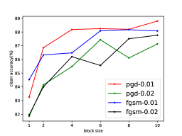
(a) Influence on clean accuracy

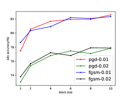
(b) Influence on adversarial accuracy

Figure B.1: The effect of block size on the accuracy. In the figure, we show the clean accuracy and the adversarial accuracy of the mean classifier under PGD and FGSM attack with $\epsilon=0.01$ and $\epsilon=0.02$. The block size is choosen from $\{1,2,4,6,8,10\}$. (a) The influence on the clean accuracy; (b) The influence on the adversarial accuracy.

Attack	$\epsilon$	Type	$\lambda$
			$0$	$0.002$	$0.005$	$0.01$	$0.02$
PGD	0.01	Clean	$84.07$	$\bm{85.65}$	$85.48$	$85.52$	$58.53$
		Adv	$78.49$	$\bm{79.55}$	$79.39$	$79.41$	$79.44$
	0.02	Clean	$81.87$	$81.91$	$81.93$	$\bm{82.08}$	$81.97$
		Adv	$73.01$	$73.05$	$73.07$	$\bm{73.16}$	$73.07$
FGSM	0.01	Clean	$84.61$	$84.53$	$\bm{84.95}$	$84.58$	$84.55$
		Adv	$78.70$	$78.64$	$\bm{79.18}$	$78.70$	$78.63$
	0.02	Clean	$80.47$	$80.48$	$80.39$	$80.44$	$\bm{82.09}$
		Adv	$72.45$	$72.45$	$72.36$	$72.41$	$\bm{73.87}$

Table B.1: Results of experiments on the regularizer on data set CIFAR-100. In this table, we list the clean accuracy (Clean) and adversarial accuracy (Adv) of the mean classifier under the PGD and FGSM attack with $\epsilon=0.01$ and $\epsilon=0.02$. $\lambda$ is chosen from $\{0,0.002,0.005,0.01,0.02\}$, and $\lambda=0$ indicates no regularizer.

Table B.1 shows that the $F$-norm regularizer helps to improve the adversarial robustness of the model, which agrees with our Theorem 24.

B.2 Effect of Block Size

Figure B.1 records the influence of block size on the clean accuracy and the adversarial accuracy of the model, from which we can see that a larger block size will yield better adversarial accuracy.

References

- Awasthi et al. (2020) Pranjal Awasthi, Natalie Frank, and Mehryar Mohri. Adversarial learning guarantees for linear hypotheses and neural networks. In ICML, volume 119, pages 431–441, 2020.
- Carlini and Wagner (2017) Nicholas Carlini and David A. Wagner. Towards evaluating the robustness of neural networks. In SP, pages 39–57, 2017.
- Chen et al. (2020) Ting Chen, Simon Kornblith, Mohammad Norouzi, and Geoffrey E. Hinton. A simple framework for contrastive learning of visual representations. In ICML, volume 119, pages 1597–1607, 2020.
- Gao and Wang (2021) Qingyi Gao and Xiao Wang. Theoretical investigation of generalization bounds for adversarial learning of deep neural networks. Journal of Statistical Theory and Practice, 15(2):51, 2021.
- Gidaris et al. (2018) Spyros Gidaris, Praveer Singh, and Nikos Komodakis. Unsupervised representation learning by predicting image rotations. In ICLR, 2018.
- Goodfellow et al. (2015) Ian J. Goodfellow, Jonathon Shlens, and Christian Szegedy. Explaining and harnessing adversarial examples. In ICLR, 2015.
- He et al. (2020) Kaiming He, Haoqi Fan, Yuxin Wu, Saining Xie, and Ross B. Girshick. Momentum contrast for unsupervised visual representation learning. In CVPR, pages 9726–9735, 2020.
- Ho and Vasconcelos (2020) Chih-Hui Ho and Nuno Vasconcelos. Contrastive learning with adversarial examples. In NeurIPS, 2020.
- Jiang et al. (2020) Ziyu Jiang, Tianlong Chen, Ting Chen, and Zhangyang Wang. Robust pre-training by adversarial contrastive learning. In NeurIPS, 2020.
- Kim et al. (2020) Minseon Kim, Jihoon Tack, and Sung Ju Hwang. Adversarial self-supervised contrastive learning. In NeurIPS, 2020.
- Krizhevsky and Hinton (2009) Alex Krizhevsky and Geoffrey Hinton. Learning multiple layers of features from tiny images. 2009.
- Kurakin et al. (2017) Alexey Kurakin, Ian J. Goodfellow, and Samy Bengio. Adversarial examples in the physical world. In ICLR, 2017.
- Ledoux and Talagrand (2013) Michel Ledoux and Michel Talagrand. Probability in Banach Spaces: isoperimetry and processes. Springer Science & Business Media, 2013.
- Li and Liu (2023) Boqi Li and Weiwei Liu. Wat: Improve the worst-class robustness in adversarial training, 2023.
- Li et al. (2022) Xiyuan Li, Xin Zou, and Weiwei Liu. Defending against adversarial attacks via neural dynamic system. In NeurIPS, 2022.
- Ma et al. (2022) Xinsong Ma, Zekai Wang, and Weiwei Liu. On the tradeoff between robustness and fairness. In NeurIPS, 2022.
- Madry et al. (2018) Aleksander Madry, Aleksandar Makelov, Ludwig Schmidt, Dimitris Tsipras, and Adrian Vladu. Towards deep learning models resistant to adversarial attacks. In ICLR, 2018.
- Maiorov and Pinkus (1999) Vitaly Maiorov and Allan Pinkus. Lower bounds for approximation by MLP neural networks. Neurocomputing, 25(1-3):81–91, 1999.
- Mao et al. (2020) Chengzhi Mao, Amogh Gupta, Vikram Nitin, Baishakhi Ray, Shuran Song, Junfeng Yang, and Carl Vondrick. Multitask learning strengthens adversarial robustness. In ECCV, pages 158–174, 2020.
- Mohri et al. (2012) Mehryar Mohri, Afshin Rostamizadeh, and Ameet Talwalkar. Foundations of Machine Learning. Adaptive computation and machine learning. MIT Press, 2012.
- Montasser et al. (2019) Omar Montasser, Steve Hanneke, and Nathan Srebro. VC classes are adversarially robustly learnable, but only improperly. In COLT, pages 2512–2530, 2019.
- Moosavi-Dezfooli et al. (2016) Seyed-Mohsen Moosavi-Dezfooli, Alhussein Fawzi, and Pascal Frossard. Deepfool: A simple and accurate method to fool deep neural networks. In CVPR, pages 2574–2582, 2016.
- Neyshabur et al. (2015) Behnam Neyshabur, Ryota Tomioka, and Nathan Srebro. Norm-based capacity control in neural networks. In COLT, volume 40, pages 1376–1401, 2015.
- Noroozi and Favaro (2016) Mehdi Noroozi and Paolo Favaro. Unsupervised learning of visual representations by solving jigsaw puzzles. In ECCV, volume 9910, pages 69–84, 2016.
- Nozawa et al. (2020) Kento Nozawa, Pascal Germain, and Benjamin Guedj. Pac-bayesian contrastive unsupervised representation learning. In UAI, volume 124, pages 21–30, 2020.
- Saunshi et al. (2019) Nikunj Saunshi, Orestis Plevrakis, Sanjeev Arora, Mikhail Khodak, and Hrishikesh Khandeparkar. A theoretical analysis of contrastive unsupervised representation learning. In ICML, volume 97, pages 5628–5637, 2019.
- Schmidt et al. (2018) Ludwig Schmidt, Shibani Santurkar, Dimitris Tsipras, Kunal Talwar, and Aleksander Madry. Adversarially robust generalization requires more data. In NeurIPS, pages 5019–5031, 2018.
- Szegedy et al. (2014) Christian Szegedy, Wojciech Zaremba, Ilya Sutskever, Joan Bruna, Dumitru Erhan, Ian J. Goodfellow, and Rob Fergus. Intriguing properties of neural networks. In ICLR, 2014.
- Wainwright (2019) Martin J. Wainwright. High-dimensional statistics: A non-asymptotic viewpoint, volume 48. Cambridge University Press, 2019.
- Wang and Liu (2022) Zekai Wang and Weiwei Liu. Robustness verification for contrastive learning. In ICML, pages 22865–22883, 2022.
- Xu and Liu (2022) Jingyuan Xu and Weiwei Liu. On robust multiclass learnability. In NeurIPS, 2022.
- Yin et al. (2019) Dong Yin, Kannan Ramchandran, and Peter L. Bartlett. Rademacher complexity for adversarially robust generalization. In ICML, volume 97, pages 7085–7094, 2019.
- Zhang et al. (2017) Chiyuan Zhang, Samy Bengio, Moritz Hardt, Benjamin Recht, and Oriol Vinyals. Understanding deep learning requires rethinking generalization. In ICLR, 2017.
- Zhang et al. (2019) Hongyang Zhang, Yaodong Yu, Jiantao Jiao, Eric P. Xing, Laurent El Ghaoui, and Michael I. Jordan. Theoretically principled trade-off between robustness and accuracy. In ICML, volume 97, pages 7472–7482, 2019.