Distributed Empirical Risk Minimization With Differential Privacy

Abstract

This work studies the distributed empirical risk minimization (ERM) problem under differential privacy (DP) constraint. Standard distributed algorithms achieve DP typically by perturbing all local subgradients with noise, leading to significantly degenerated utility. To tackle this issue, we develop a class of private distributed dual averaging (DDA) algorithms, which activates a fraction of nodes to perform optimization. Such subsampling procedure provably amplifies the DP guarantee, thereby achieving an equivalent level of DP with reduced noise. We prove that the proposed algorithms have utility loss comparable to centralized private algorithms for both general and strongly convex problems. When removing the noise, our algorithm attains the optimal $\mathcal{O}(1/t)$ convergence for non-smooth stochastic optimization. Finally, experimental results on two benchmark datasets are given to verify the effectiveness of the proposed algorithms.

, ,

1 Introduction

Consider a group of $n$ nodes, where each node $i$ has a local dataset ${D}_{i}=\{\xi_{i}^{(1)},\dots,\xi_{i}^{(q)}\}$ that contains a finite number $q$ of data samples. The nodes are connected via a communication network. They aim to collaboratively solve the empirical risk minimization (ERM) problem, where the machine learning models are trained by minimizing the average of empirical prediction loss over known data samples. Formally, the optimization problem is given by

$$\min_{x\in\mathbb{R}^{m}}\left\{F(x):=\frac{1}{n}\sum_{i=1}^{n}f_{i}(x)+h(x)\right\},$$ (1)

where $f_{i}(x)=\frac{1}{q}\sum_{j=1}^{q}{l}_{i}(x,\xi_{i}^{(j)})$ represents the empirical risk on node $i$, $l_{i}(x,\xi)$ is the loss of the model $x$ over the data instance $\xi$, and $h(x)$ is the regularization term shared across the nodes. This setup has been commonly considered in machine learning [18], where $h(x)$ is used to promote sparsity or model the constraints.

As the loss and its gradient in ERM are characterized by data samples, potential privacy issues arise when the datasets are sensitive [2]. In particular, when $l_{i}$ is the hinge loss, the solution to Problem (1), i.e., support vector machine (SVM), in its dual form typically discloses data points [2]. Advanced attacks such as input data reconstruction [43] and attribute inference [22] can extract private information from the gradients. To defend privacy attacks, differential privacy (DP) has become prevalent in cryptography and machine learning [8, 1], due to its precise notion and computational simplicity. Informally, DP requires the outcome of an algorithm to remain stable under any possible changes to an individual in the database, and therefore protects individuals from attacks that try to steal the information particular to them. The DP constraint induces a tradeoff between privacy and utility in learning algorithms [2, 16, 3, 29].

In this work, we are interested in solving Problem (1) while providing rigorous DP guarantee for each data sample in $D:=\cup_{i=1}^{n}D_{i}$.

1.1 Related work

For problems without regularization, i.e., $h\equiv 0$, the authors in [14] developed a differentially private distributed gradient descent (DGD) algorithm by perturbing the local output with Laplace noise. Notably, the learning rate is designed to be linearly decaying such that the sensitivity of the algorithm also decreases linearly. Then, one can decompose the prescribed DP parameter $\varepsilon$ into a sequence $\{\varepsilon_{t}\}_{t\geq 1}$, such that $\sum_{\tau=1}^{\infty}\varepsilon_{\tau}=\varepsilon$ and the operation at each time instant $t$ can be made $\varepsilon_{t}$-DP. However, such choice of learning rate slows down the convergence dramatically and results in a utility loss in the order of $\mathcal{O}(m/\varepsilon^{2})$, where $m$ denotes the dimension of the decision variable. Under the more reasonable learning rate $\Theta(1/\sqrt{t})$, the utility loss can be improved to $\mathcal{O}\left(\sqrt[4]{{mn^{2}}/{\varepsilon}}\right)$ [12], where $n$ denotes the number of nodes. Along this line of research, the authors in [42, 34, 11] extended the algorithm to time-varying objective functions, and the authors in [6] advanced the convergence rate to linear based on an additional gradient-tracking scheme. The authors in [30] developed a distributed algorithm with DP for stochastic aggregative games. The differentially private distributed optimization problem with coupled equality constraints has been studied in [4]. In these works, however, $\varepsilon$-DP is proved only for each iteration, leading to a cumulative privacy loss of $t\varepsilon$ after $t$ iterations. To attenuate the noise effect while ensuring DP, the authors in [28] constructed topology-aware noise, with which each node perturbs the messages to its neighbors (including itself) with different perturbations whose weighted sum is $0$.

For federated learning (FL) with heterogeneous data, the authors in [13] developed a personalized linear model training algorithm with DP. In [24], general models were considered. In particular, the subsampling of users and local data has been explicitly considered to amplify the DP guarantee and improve the utility.

To tackle regularized learning problems, the alternating direction method of multipliers (ADMM) has been used to design distributed algorithms with DP [40, 37, 41]. However, an explicit tradeoff analysis between privacy and utility was missing. The authors in [32] investigated the privacy guarantee produced not only by random noise injection but also by mixup [38], i.e., a random convex combination of inputs. Approximate DP and advanced composition [15] were used to keep track of the cumulative privacy loss. The privacy–utility tradeoff in linearized ADMM and DGD were captured by the bound $\mathcal{O}\left({m}/{(\sqrt{n}\varepsilon)}\right)$.

To summarize, existing private distributed optimization algorithms applied to Problem (1) typically require each node to make a gradient query to the local dataset at each time instant. Since the sizes of local datasets are considerably smaller than that of the original dataset, local gradient queries have larger sensitivity parameters than that in centralized settings. Therefore, private distributed optimization paradigms in the literature typically employed a larger magnitude of noise to secure the same level of DP, and suffered from relatively low utility. Recently, an asynchronous DGD method with DP was developed in [35], which achieved a lower utility loss. The algorithm assumed that each local mini-batch is a subset of data instances uniformly sampled from the overall dataset without replacement, which appears to be restrictive in distributed settings.

1.2 Contribution

We develop a class of differentially private distributed dual averaging (DDA) algorithms for solving Problem (1). At each iteration, a fraction of nodes is activated uniformly at random to perform local stochastic subgradient query and local update with perturbed subgradient. Such subsampling procedure provably amplifies the DP guarantee and therefore helps achieve the same level of DP with weaker noise. To ensure a user-defined level of DP, we provide sufficient conditions on the noise variance in Theorem 1, which admits a smaller bound of variance than existing results.

The properties of the proposed algorithms in terms of convergence and the privacy-utility tradeoff are analyzed. First, a non-asymptotic convergence analysis is conducted for dual averaging with inexact oracles under general choices of hyperparameters, and the results are summarized in Theorem 2. This piece of result illustrates how the lack of global information and the DP noise in private DDA quantitively affect the convergence, which lays the foundation for subsequent analysis. Then, we investigate the convergence rate of the non-private (noiseless) version of DDA for both strongly convex and general convex objective functions under two sets of hyperparameters in Corollaries 3.2 and 3.4, respectively. We remark that Corollary 3.2 advances the best known convergence rate of DDA for nonsmooth stochastic optimization, i.e., $\mathcal{O}(1/\sqrt{t})$, to $\mathcal{O}(1/t)$. The key to obtaining the improved rate is the use of a new class of parameters.

The privacy–utility tradeoff of the proposed algorithm is examined in Corollaries 3.5 and 3.6. In particular, when the objective function is non-smooth and strongly convex, the utility loss is characterized by $\mathcal{O}(m\iota^{2}/(q^{2}\varepsilon^{2}))$, where $m$, $\iota$, $q$, $\varepsilon$ denote the variable dimension, node sampling ratio, number of samples per node, and DP parameter, respectively. For comparison, we present in Table 1 a comparison of some of the most relevant works.

Finally, we verify the effectiveness of the proposed algorithms via distributed SVM on two open-source datasets. Several comparison results are also presented to support our theoretical findings.

1.3 Outline

The rest of the paper is organized as follows. Section 2 introduces some preliminaries. We present our algorithms and their theoretical properties in Section 3, whose proofs are postponed to Section 4. Some experimental results are given in Section 5. Section 6 concludes the paper.

Table 1: A Comparison of Some Related Works

	Privacy	Noise	Perturbed	Utility Upper Bound		Non-smooth
			Term	Convex	Strongly Convex	Regularizer
[24] (FL)	($\varepsilon$, $\delta$)-DP	Gaussian	Gradient	$\mathcal{O}\left(\frac{\sqrt{m}}{nq\varepsilon}\right)$	$\mathcal{O}\left(\frac{m}{n^{2}q^{2}\varepsilon^{2}}\right)$	No
[14]	$\varepsilon$-DP	Laplace	Output	–	$\mathcal{O}(\frac{m}{\varepsilon^{2}})$	No
[32] (ADMM)	$(\varepsilon,\delta)$-DP	Gaussian	Output	$\mathcal{O}\left(\frac{{n}^{3/2}\varepsilon}{m}\right)$	–	No
[32] (DGD)	$(\varepsilon,\delta)$-DP	Gaussian	Gradient	${\mathcal{O}}(\frac{m}{\sqrt{n}\varepsilon})$	–	No
[35]	$(\varepsilon,\delta)$-DP	Gaussian	Gradient	${\mathcal{O}}(\frac{\sqrt{m}}{q\varepsilon})$	–	No
This work	($\varepsilon$, $\delta$)-DP	Gaussian	Gradient	$\mathcal{O}\left(\frac{\sqrt{m\iota}}{q\varepsilon}\right)$	$\mathcal{O}\left(\frac{m\iota^{2}}{q^{2}\varepsilon^{2}}\right)$	Yes

2 Preliminaries

2.1 Basic setup

We consider the distributed ERM in (1), in which $h$ is a closed convex function with non-empty domain $\mbox{dom}(h)$. Examples of $h(x)$ include $l_{1}$-regularization, i.e., $h(x)=\lambda\lVert x\rVert_{1},\lambda>0$, and the indicator function of a closed convex set. The regularization term $h$ and the loss functions $l_{i}$ for all $i=1,\dots,n$ satisfy the following assumptions.

Assumption 1.

i) $h(\cdot)$ is a proper closed convex (strongly convex) function with modulus $\mu=0$ (resp. $\mu>0$), i.e., for any $x,y\in dom(h)$,

$$h(\alpha x+(1-\alpha)y)\leq\alpha h(x)+(1-\alpha)h(y)-\frac{\mu\alpha(1-\alpha)}{2}\lVert x-y\rVert^{2};$$

ii) each $l_{i}(\cdot,\xi_{i})$ is convex on $dom(h)$.

When $q=1$, Problem (1) reduces to a deterministic distributed optimization problem. In Problem (1), the information exchange only occurs between connected nodes. Similar to existing research [23, 7], we use a doubly stochastic matrix $W\in[0,1]^{n\times n}$ to encode the network topology and the weights of connected links at time $t$. In particular, its $(i,j)$-th entry, $w_{ij}$, denotes the weight used by $i$ when counting the message from $j$. When $w_{ij}=0$, nodes $i$ and $j$ are disconnected.

2.2 Conventional DDA

The DDA algorithm originally proposed by [7] can be applied to solve Problem (1). In particular, let $d(\cdot)\geq 0$ be a strongly convex function with modulus $1$ on $\mbox{dom}(h)$. Each node, starting with $z_{i}^{(1)}=0$, iteratively generates $\{z_{i}^{(t)},x_{i}^{(t)}\}_{t\geq 1}$ according to

$$\begin{split}x_{i}^{(t)}=\operatorname*{argmin}_{x\in\mathbb{R}^{m}}\left\{\langle z_{i}^{(t)},x\rangle+t(h(x))+\gamma_{t}d(x)\right\}\end{split}$$ (2)

and

$$z_{i}^{(t+1)}=\sum_{j=1}^{n}w_{ij}\left(z_{j}^{(t)}+\hat{g}_{j}^{(t)}\right),$$ (3)

where $\{\gamma_{t}\}_{t\geq 1}$ is a non-decreasing sequence of parameters, $w_{ij}$ is the $(i,j)$-th entry of matrix $W$, $\hat{g}_{j}^{(t)}\in\partial l_{j}(x_{j}^{(t)},\xi_{j}^{(t)})$ denotes the stochastic subgradient of local loss over $x_{j}^{(t)}$ with $\xi_{j}^{(t)}$ uniformly sampled from $D_{j}$, and $\partial l_{j}(x_{j}^{(t)},\xi_{j}^{(t)})$ represents the corresponding subdifferential. Throughout the process, each node only passes $z_{i}$ to its immediate neighbors and updates $x_{i}$ according to (2). Existing DDA algorithms, when applied to solve Problem (1), converge as $\mathcal{O}(1/\sqrt{t})$ [7, 5].

2.3 Threat model and DP

In a distributed optimization algorithm, messages bearing information about the local training data are exchanged among the nodes, which leads to privacy risk. In this work, we consider the following two types of attackers.

• Honest-but-curious nodes are assumed to follow the algorithm to perform communication and computation. However, they may record the intermediate results to infer the sensitive information about the other nodes.

• External eavesdroppers stealthily listen to the private communications between the nodes.

By collecting the confidential messages, the attackers are abele to infer private information about the users [43]. To defend them, we employ tools from DP. Indeed, DP has been recognized as the gold standard in quantifying individual privacy preservation for randomized algorithms. It refers to the property of a randomized algorithm that the presence or absence of an individual in a dataset cannot be distinguished based on the output of the algorithm. Formally, we introduce the following definition of DP for distributed optimization algorithms [41].

Definition 1.

Consider a communication network, in which each node has its own dataset $D_{i}$. Let $\{z_{i}^{(t)}:i=1,\dots,n\}$ denote the set of messages exchanged among the nodes at iteration $t$. A distributed algorithm satisfies $(\varepsilon,\delta)$-DP during $T$ iterations, if for every pair of neighboring datasets $D=\cup_{i=1}^{n}D_{i}$ and $D^{\prime}=\cup_{i=1}^{n}D^{\prime}_{i}$, and for any set of possible outputs $\mathcal{O}$ during $T$ iterations we have

$$\begin{split}&Pr[\{z_{i}^{(t)},i=1,\dots,n\}_{t=1}^{T}\in\mathcal{O}|D]\\ &\leq e^{\varepsilon}Pr[\{z_{i}^{(t)},i=1,\dots,n\}_{t=1}^{T}\in\mathcal{O}|D^{\prime}]+\delta.\end{split}$$

3 Differentially private DDA algorithm

In this section, we develop the differentially private DDA algorithm, followed by its privacy-preserving and convergence properties.

3.1 Node subsampling in distributed optimization

As explained in Section 1, parallelized local gradient queries in distributed optimization necessitate stronger noise to achieve DP and therefore deteriorate utility. To circumvent this problem, we only activate a random fraction of the nodes at each time instant to perform averaging and local optimization. This allows us to amplify the privacy of the algorithm, and thereby achieving the same level of DP with noise weaker than in existing works.

Definition 2.

For every $t\geq 1$, an integer number of $n\iota$ nodes are sampled uniformly at random with some $\iota\in(0,1]$.

The sampling procedure gives rise to a time-varying stochastic communication network. Slightly adjusted to the notation in Section 2.1, we let $W^{(t)}\in[0,1]^{n\times n}$ be a random gossip matrix at time $t$, where the $(i,j)$-th entry, $w_{ij}^{(t)}$, denotes the weight of the link $(i,j)$ at time $t$. Denote by $\mathcal{N}^{(t)}$ and $\mathcal{N}_{i}^{(t)}:=\{j|j\neq i,w_{ij}^{(t)}>0\}$ the set of activated nodes and the set of $i$’s neighbors at time $t$, respectively. It is worthwhile to point out that $W^{(t)}$ and $\iota$ are dependent. That is, we have $w_{ij}^{(t)}>0$ for $i\in\mathcal{N}^{(t)}$ and $j\in\mathcal{N}_{i}^{(t)}$, and $w_{ij}^{(t)}=0$ otherwise.

For the gossip matrix $W^{(t)}$, we assume the following standard condition [20].

Assumption 2.

For every $t\geq 1$, i) $W^{(t)}$ is doubly stochastic; ii) $W^{(t)}$ is independent of the random events that occur up to time $t-1$; and iii) there exists a constant $\beta\in(0,1)$ such that

$$\sqrt{\rho\left(\mathbb{E}_{W}\left[{W^{(t)}}^{T}W^{(t)}\right]-\frac{\mathbf{1}\mathbf{1}^{T}}{n}\right)}\leq\beta,$$ (4)

where $\rho(\cdot)$ denotes the spectral radius and the expectation $\mathbb{E}[\cdot]$ is taken with respect to the distribution of $W^{(t)}$ at time $t$.

3.2 Private DDA with stochastic subgradient perturbation

Next, we introduce a differentially private DDA algorithm presented as Algorithm 1.

The update for the local dual variable $z_{i}^{(t)}$ reads

$$z_{i}^{(t+1)}=\sum_{j=1}^{n}w_{ij}^{(t)}\left(z_{j}^{(t)}+a_{t}\eta_{j}^{(t)}\zeta_{j}^{(t)}\right),$$ (5)

where $\zeta_{j}^{(t)}=\hat{g}_{j}^{(t)}+\nu_{j}^{(t)}$, $\nu_{j}^{(t)}\sim\mathcal{N}(0,\sigma^{2}I)$, $\hat{g}_{j}^{(t)}\in\partial l_{j}(x_{j}^{(t)},\xi_{j}^{(t)})$ with $\xi_{j}^{(t)}$ uniformly sampled from $D_{j}$, $\eta_{i}^{(t)}$ indicates whether node $i$ performs local update at time $t$, i.e.,

$$\eta_{i}^{(t)}=\left\{\begin{aligned} &1,&\mbox{if}\,\,i\,\,\mbox{active}\\ &0,&\mbox{ otherwise}\end{aligned}\right.$$

and $\{a_{t}>0\}_{t\geq 1}$ is a sequence of non-decreasing parameters. The non-decreasing property of $\{a_{t}\}_{t\geq 1}$ is motivated by that, when the objective exhibits some desirable properties, e.g., strong convexity, assigning heavier weights to fresher subgradients can speed up convergence [21, 27]. In the special case where $a_{t}=1$, $\eta_{i}^{(t)}=1$ and $\sigma=0$, (5) reduces to the conventional update in (3).

Equipped with (5), node $i$, active at time $t$, can perform a local computation to derive its estimate about the global optimum:

$$\begin{split}{x}_{i}^{(t+1)}=\operatorname*{argmin}_{x\in\mathbb{R}^{m}}\left\{\langle z_{i}^{(t+1)},x\rangle+\iota A_{t+1}h(x)+\gamma_{t+1}d(x)\right\},\end{split}$$ (6)

where $\iota$ is defined in Definition 2, $A_{t}=\sum_{\tau=1}^{t}a_{\tau}$ and $\{\gamma_{t}\}_{t\geq 1}$ is a non-decreasing sequence of positive parameters. By convention, we let $A_{0}=a_{0}=0$ and $\gamma_{0}=0$.

Algorithm 1 Differentially Private DDA

1:Input: $\mu\geq 0$, $a>0$, a strongly convex function $d$ with modulus $1$ on $\mbox{dom}(h)$, and $T>0$

2:Output: $\tilde{x}_{i}^{(T)}=A_{T}^{-1}\sum_{t=1}^{T}a_{t}x_{i}^{(t)}$

3:Initialize: set $z_{i}^{(1)}=0$ and identify $x_{i}^{(1)}$ according to (6) for all $i=1,\dots,n$

4:for $t=1,2,\dots,T$ do

5: For active nodes $i\in\mathcal{N}^{(t)}$:

6:   $\xi_{i}^{(t)}\sim\text{Uniform}\{1,\dots,q\}$ and $\nu_{i}{(t)}\sim\mathcal{N}(0,\sigma^{2}I)$

7:   release $\hat{g}_{i}^{(t)}+\nu_{i}^{(t)}$

8:   collect $z_{j}^{(t)}+a_{t}(\hat{g}_{j}^{(t)}+\nu_{j}^{(t)})$ from all nodes $j\in\mathcal{N}_{i}^{(t)}$

9:   update $z_{i}^{(t+1)}$ by (5)

10:   compute $x_{i}^{(t+1)}$ by (6)

11: For inactive nodes $i\notin\mathcal{N}^{(t)}$:

12:   set $z_{i}^{(t+1)}=z_{i}^{(t)}$ and $x_{i}^{(t+1)}=x_{i}^{(t)}$

13:end for

For general regularization $h(x)$, the update in (6) requires the knowledge of $\iota$. This requirement is necessary due to technical reasons. More precisely, due to node sampling, the term $\langle z_{i}^{(t+1)},x\rangle$ in (6) serves as a linear approximation of $\iota f_{i}(x)/n$ rather than $f_{i}(x)/n$ in standard DDA [7]. Thus, one scales up $h(x)$ also with $\iota$ in (6) in order to solve the original problem in (1). In the special case where $h(x)$ is the indicator function of a convex set, the knowledge of $\iota$ is not needed since $\iota h(x)\equiv h(x)$.

The overall procedure is summarized in Algorithm 1. Each node $i=1,\dots,n$ initializes $z_{i}^{(1)}=0$ in Step 1. At each time instant $t$, only active nodes $i\in\mathcal{N}^{(t)}$ update $z_{i}^{(t+1)}$ and $x_{i}^{(t+1)}$ by following Steps 3–7. In particular, each active node computes and then perturbs the local stochastic subgradient in Step 3 and 4, respectively, followed by the information exchange with neighboring nodes in Step 5. Then, $z_{i}^{(t+1)}$ and $x_{i}^{(t+1)}$ are updated in Steps 6 and 7. For inactive nodes at each time instant $t$, they simply set $z_{i}^{(t+1)}=z_{i}^{(t)}$ and $x_{i}^{(t+1)}=x_{i}^{(t)}$.

Remark 1.

There are two common approaches to achieve DP for optimization methods. The first type disturbs the output of a non-private algorithm [39], and the second type perturbs the subgradient [2, 29]. The former involves recursively estimating the (time-varying) sensitivity of updates [31]. This makes the propagation of DP noise and its effect on convergence difficult to quantify [31]. In this work, we adopt the latter approach in Algorithm 1, where we introduce Gaussian noise to perturb the stochastic subgradient $\hat{g}_{i}$. By leveraging the time-invariant sensitivity of the gradient query, we can effectively conduct both privacy and utility analyses in the presence of non-smooth regularization. It is worth noting that, in this scenario, the step-size scheduling rule allows for control over utility.

3.3 Privacy analysis

To establish the privacy-preserving property of Algorithm 1, we make the following assumption.

Assumption 3.

Each $l_{i}(\cdot,\xi_{i})$ is $L$-Lipschitz, i.e., for any $x,y\in dom(h)$,

$$\lvert l_{i}(x,\xi_{i})-l_{i}(y,\xi_{i})\rvert\leq L\lVert x-y\rVert.$$

By Assumption 3, we readily have that each $f_{i}(\cdot)$ is $L$-Lipschitz. Next, we state the privacy guarantee for Algorithm 1. The proof can be found in Section 4.1.

Theorem 1.

Suppose Assumption 3 is satisfied, and a random fraction of the nodes with ratio $\iota\in(0,1]$ is active at each time instant. Given parameters ${q}$, $\varepsilon\in(0,1]$, and $\delta_{0}\in(0,1]$, if

$$\sigma^{2}\geq\frac{32\iota^{2}L^{2}T\log(2/\delta_{0})}{q^{2}\varepsilon^{2}}$$

and $T\geq 5q^{2}\varepsilon^{2}/(4\iota^{2})$, then Algorithm 1 is $(\varepsilon,\delta)$-DP for some constant $\delta\in(0,1]$.

Remark 3.1.

A few remarks on the results in Theorem 1 are in order:

• It can be verified from the proof of Theorem 1 that Algorithm 1 is ($\hat{\varepsilon},\delta$)-DP after $t\leq T$ iterations with

  $$\hat{\varepsilon}\leq\sqrt{\frac{3t}{5T}}{\varepsilon}+\frac{t}{5T}{\varepsilon^{2}}.$$ (7)

• Theorem 1 emphasizes that, to achieve a prescribed privacy budget during $T$ iterations, the noise variance $\sigma^{2}$ is related to the DP parameters $(\varepsilon,\delta)$, the Lipschitz constant $L$ of the loss, the number of samples per local dataset, and the iteration number $T$. Notably, the lower bound for variance is weighted by $\iota^{2}\leq 1$, meaning that the same level of DP can be achieved with reduced noise.

3.4 Privacy–utility tradeoff

Next, we perform a non-asymptotic analysis of Algorithm 1, followed by an explicit privacy–utility tradeoff.

Motivated by [7], we define an auxiliary sequence of variables:

$$y^{(t+1)}=\operatorname*{argmin}_{x\in\mathbb{R}^{m}}\left\{\langle\overline{z}^{(t+1)},x\rangle+\iota A_{t+1}h(x)+\gamma_{t+1}d(x)\right\},$$ (8)

where $\overline{z}^{(t)}=\frac{1}{n}\sum_{i=1}^{n}z_{i}^{(t)}$ and $\{z_{i}^{(t)}:i=1,\dots,n\}_{t\geq 1}$ are generated by Algorithm 1. The convergence property of $y^{(t)}$ is summarized in Theorem 2, whose proof is provided in Section 4.2.

Theorem 2.

Suppose Assumptions 1, 2, and 3 are satisfied. For all $t\geq 1$, we have

$$\begin{split}&A_{t}\mathbb{E}[F(\tilde{y}^{(t)})-F(x^{*})]\\ &\leq\frac{\gamma_{t}}{\iota}d(x^{*})+\sum_{\tau=1}^{t}\frac{a_{\tau}^{2}}{\mu\iota A_{\tau}+\gamma_{\tau}}\Big{(}M+\frac{m\iota\sigma^{2}}{2}+\frac{2\sqrt{m\iota}L\sigma}{1-\beta}\Big{)},\end{split}$$ (9)

where $\sigma$ is defined in Theorem 1, $\tilde{y}^{(t)}=A_{t}^{-1}\sum_{\tau=1}^{t}a_{\tau}y^{(\tau)}$, $M={\iota L^{2}}/{2}+{2\sqrt{\iota}L^{2}}/{(1-\beta)}$, and the expectation is over the randomness of the algorithm.

From the error bound in (9), we observe that the last two terms are contributed by the noise. How the noise affects the error bound is determined in part by the hyperparameters of the algorithm. Next, we first investigate the choices of $a_{t}$ that lead to optimal convergence rates for Algorithm 1 with $\sigma=0$; the results for strongly convex and general convex functions are presented in Corollaries 3.2 and 3.4, whose proofs are given in Appendices C and D, respectively.

Corollary 3.2.

Suppose Assumptions 2 and 3 are satisfied. In addition, Assumption 1 holds with $\mu>0$, i.e., $h(x)$ is $\mu$-strongly convex. If $\sigma=0$,

$$a_{t}=t\ \ \mbox{and}\ \ \gamma_{t}=0,$$

then for all $t\geq 1$, and $i=1,\dots,n$, we have

$$\begin{split}\frac{1}{n}\sum_{i=1}^{n}\mathbb{E}[\lVert\tilde{x}_{i}^{(t)}-x^{*}\rVert^{2}]\leq\frac{16}{t+1}\left(\frac{L^{2}(\log t+1)}{\mu^{2}\iota(1-\beta)^{2}t}+\frac{M}{\mu^{2}\iota}\right),\end{split}$$ (10)

where $\tilde{x}_{i}^{(t)}=A_{t}^{-1}\sum_{\tau=1}^{t}a_{\tau}x_{i}^{(\tau)}$ and $M$ is a positive constant given in Theorem 2.

Remark 3.3.

Corollary 3.2 indicates that the non-private version of Algorithm 1, i.e., $\sigma=0$, attains the optimal convergence rate $\mathcal{O}(1/t)$ when Problem (1) is strongly convex. Compared to the algorithm in [36], where the authors focused on constrained problems, the proposed algorithm handles general non-smooth regularizers. Furthermore, the results can be extended to the case where each $f_{i}(x)$ but not $h(x)$ is strongly convex by following a similar idea in [20].

Corollary 3.4.

Suppose Assumptions 2 and 3 are satisfied. In addition, Assumption 1 holds with $\mu=0$, i.e., $h(x)$ is general convex. If $\sigma=0$,

$$a_{t}=1\ \ \mbox{and}\ \ \gamma_{t}=\gamma\sqrt{t},$$

then for all $t\geq 1$, and $i=1,\dots,n$, we have

$$\mathbb{E}\left[F(\tilde{y}^{(t)})-F(x^{*})\right]\leq\frac{d(x^{*})+2\iota M}{\iota\gamma\sqrt{t}},$$ (11)

where $\tilde{y}^{(t)}=t^{-1}\sum_{\tau=1}^{t}y^{(\tau)}$ and $M$ is a positive constant given in Theorem 2. In addition, for all $t\geq 1$, and $i=1,\dots,n$, we have

$$\frac{1}{n}\sum_{i=1}^{n}\mathbb{E}[\lVert\tilde{x}_{i}^{(t)}-\tilde{y}^{(t)}\rVert]\leq\frac{2L\sqrt{\iota}}{\gamma(1-\beta)\sqrt{t}},$$ (12)

where $\tilde{x}_{i}^{(t)}=t^{-1}\sum_{\tau=1}^{t}{x}_{i}^{(\tau)}$.

Under the same hyperparameters, we study the privacy–utlity tradeoff of Algorithm 1 with $\sigma\neq 0$ for strongly convex and general convex functions in Corollaries 3.5 and 3.6, whose proofs are presented in Appendices E and F, respectively.

Corollary 3.5.

Suppose Assumptions 2 and 3 are satisfied. In addition, Assumption 1 holds with $\mu>0$, i.e., $h(x)$ is $\mu$-strongly convex. If

$$a_{t}={t},\ \ \ \gamma_{t}=0,$$

and $\beta\in(1-\sqrt{1/e},1]$, then for $T=\mathcal{O}\left(\frac{q^{2}\varepsilon^{2}}{\iota^{3}(1-\beta)^{2}m\log(1/\delta_{0})}\right)$ and $i=1,\dots,n$:

$$\begin{split}\frac{1}{n}\sum_{i=1}^{n}\mathbb{E}\left[\lVert\tilde{x}_{i}^{(T)}-x^{*}\rVert^{2}\right]\leq{\mathcal{O}}\left(\frac{m\iota^{2}L^{2}\log(1/\delta_{0})}{\mu^{2}q^{2}\varepsilon^{2}}\right),\end{split}$$ (13)

where $\tilde{x}_{i}^{(T)}=A_{T}^{-1}\sum_{t=1}^{T}a_{t}x_{i}^{(t)}$, and $\delta_{0}$ is defined in Theorem 1.

Corollary 3.6.

Suppose Assumptions 2 and 3 are satisfied. In addition, Assumption 1 holds with $\mu=0$, i.e., $h(x)$ is general convex. If

$$a_{t}=1,\ \ \gamma_{t}=\gamma\sqrt{t},$$ (14)

and $\iota\leq 1-\beta$, then the following holds for $T=\mathcal{O}\left(\frac{q^{2}\varepsilon^{2}}{\iota^{3}(1-\beta)^{2}{m\log(1/\delta_{0})}}\right)$:

$$\begin{split}\mathbb{E}[F(\tilde{y}^{(T)})-F(x^{*})]\leq\mathcal{O}\left(\frac{\left(L^{2}+d(x^{*})\right)\sqrt{m\iota\log(1/\delta_{0})}}{\gamma q\varepsilon}\right)\end{split}$$ (15)

and

$$\begin{split}\frac{1}{n}\sum_{i=1}^{n}\mathbb{E}[\lVert\tilde{x}_{i}^{(T)}-\tilde{y}^{(T)}\rVert]\leq\frac{L\sqrt{m\iota\log(1/\delta_{0})}}{\gamma q\varepsilon}\end{split}$$

for $i=1,\dots,n$, where $\tilde{y}^{(T)}=\frac{1}{T}\sum_{t=1}^{T}{y}^{(t)}$, $\tilde{x}_{i}^{(T)}=\frac{1}{T}\sum_{t=1}^{T}{x}_{i}^{(t)}$, and $\delta_{0}$ is defined in Theorem 1.

Corollaries 3.5 and 3.6 highlight that the sampling procedure lowers down the utility loss for both strongly convex and general convex problems. In particular, the utility loss in the strongly convex case becomes $\iota^{2}\approx 1/n^{2}$ times smaller than that without sampling. For general convex problems, the utility loss is $\sqrt{\iota}$ times smaller. They also suggest that the number of iterations increases in order to achieve a lower utility loss.

4 Proofs of main results

This section presents the proof of Theorems 1 and 2.

4.1 Proof of Theorem 1

We start by introducing some useful properties of DP [8, 15, 9].

Lemma 4.1 (Gaussian Mechanism).

Consider the Gaussian mechanism for answering the query $r:\mathcal{D}\rightarrow\mathbb{R}^{m}$:

$$\mathcal{\mathcal{M}}=r({D})+\nu,$$

where $D\in\mathcal{D}$, $\nu\sim\mathcal{N}(0,\sigma^{2}I)$. The mechanism $\mathcal{M}$ is ($\sqrt{2\log(2/\delta)}\Delta/\sigma,\delta$)-DP where $\Delta$ denotes the sensitivity of $r$, i.e., $\Delta=\sup_{{D},{D}^{\prime}}\lVert r({D})-r({D}^{\prime})\rVert.$

Recall from Algorithm 1 that, at each iteration, $n\iota$ nodes are sampled from $n$ nodes at random, and each activated node randomly selects a data sample from $q$ instances to compute stochastic gradients. Although such a sub-sampling is not uniform, i.e., the subsets of $n\iota$ data samples are not necessarily chosen with equal probability, it still helps amplify the privacy [9, Lemma 10].

Lemma 4.2 (Privacy Amplification by Subsampling).

Suppose $\mathcal{M}$ is an $(\varepsilon,\delta)$-DP mechanism. Let $\text{samp}_{r_{1},r_{2}}:\mathcal{U}^{r_{1}}\rightarrow\mathcal{U}^{r_{2}}$ be the subsampling operation that takes a dataset belonging to $\mathcal{U}^{r_{1}}$ as input and selects uniformly at random a subset of $r_{2}\leq r_{1}$ elements from the input dataset. Then, the mechanism

$$\mathcal{A}(\mathcal{D})=\text{samp}_{n,n\iota}(\mathcal{G}_{1},\dots,\mathcal{G}_{n})$$

where $\mathcal{G}_{i}=\text{samp}_{q,1}(\mathcal{M}(\hat{g}_{i}(\xi_{i}^{(1)})),\dots,\mathcal{M}(\hat{g}_{i}(\xi_{i}^{(q)})))$ and $\hat{g}_{i}(\xi)$ is a subgradient of $l_{i}$ evaluated over data point $\xi$ is $(\ln(1+\iota(e^{\varepsilon}-1)/q),\iota\delta/q)$-DP,

Lemma 4.3 (Composition of DP).

Given $T$ randomized algorithms $\mathcal{A}_{1},\dots,\mathcal{A}_{\tau},\dots,\mathcal{A}_{T}:\mathcal{D}\rightarrow\mathcal{R}$, each of which is ($\varepsilon_{i},\delta_{i}$)-DP with $\varepsilon_{i}\in(0,0.9]$ and $\delta_{i}\in(0,1]$. Then $\mathcal{A}:\mathcal{D}\rightarrow\mathcal{R}^{t}$ with $\mathcal{A}(\mathcal{D})=(\mathcal{A}_{1}(\mathcal{D}),\dots,\mathcal{A}_{t}(\mathcal{D}))$ is $(\tilde{\varepsilon},\tilde{\delta})$-DP with

$$\tilde{\varepsilon}=\sqrt{\sum_{i=1}^{k}2\varepsilon_{i}^{2}\log(e+\frac{\sqrt{\sum_{i=1}^{k}\varepsilon_{i}^{2}}}{\delta^{\prime}})}+\sum_{i=1}^{k}\varepsilon_{i}^{2}$$

and

$$\tilde{\delta}=1-(1-\delta^{\prime})\prod_{i=1}^{k}(1-\delta_{i})$$

for any $\delta^{\prime}\in(0,1]$.

Lemma 4.4 (Post-Processing).

Given a randomized algorithm $\mathcal{A}$ that is $(\varepsilon,\delta)$-DP. For arbitrary mapping $p$ from the set of possible outputs of $\mathcal{A}$ to an arbitrary set, $p(\mathcal{A}(\cdot))$ is $(\varepsilon,\delta)$-DP.

We are now in a position to prove Theorem 1.

DP at each time $t$: We begin by noting that the subgradient perturbation procedure at time $t$, denoted by $\mathcal{M}_{t}$, is a Gaussian mechanism whose sensitivity, by Assumption 3, is $\Delta\leq{2L}.$ Based on Lemma 4.1, $\mathcal{M}_{t}$ is ($\varepsilon_{t},\delta_{0}$)-DP with

$$\varepsilon_{t}=\frac{2L\sqrt{2\log(2/\delta_{0})}}{\sigma}$$

for any $\delta_{0}\in[0,1]$. Due to the conditions on $\sigma$ and $T$, we obtain

$$\begin{split}\varepsilon_{t}^{2}=\frac{8L^{2}\log(2/\delta_{0})}{\sigma^{2}}=\frac{q^{2}\varepsilon^{2}}{4\iota^{2}T}\leq 0.2.\end{split}$$ (16)

Denote by $\mathcal{A}_{t}$ the composition of $\mathcal{M}_{t}$ and the subsampling procedure. Upon using Lemma 4.2 and (16), we obtain that $\mathcal{A}_{t}$ is $(\varepsilon_{t}^{\prime},\iota\delta_{0}/q)$-DP with

$$\varepsilon_{t}^{\prime}=\frac{2\iota\varepsilon_{t}}{q}\geq\frac{\iota(e^{\varepsilon_{t}}-1)}{q}\geq\ln\left(1+\frac{\iota(e^{\varepsilon_{t}}-1)}{q}\right).$$

In addition, because of (16), we get $\varepsilon_{t}^{\prime}=2\iota\varepsilon_{t}/q\leq 2\varepsilon_{t}\leq 0.9$ and

$$\begin{split}&\sum_{t=1}^{T}{\varepsilon_{t}^{\prime}}^{2}=\frac{4\iota^{2}}{q^{2}}\sum_{t=1}^{T}\frac{8L^{2}\log(2/\delta_{0})}{\sigma^{2}}=\sum_{t=1}^{T}\frac{\varepsilon^{2}}{T}\leq 1.\end{split}$$ (17)

DP after $T$ iterations: Consider the composition of $\mathcal{A}_{1},\dots,\mathcal{A}_{\tau},\dots,\mathcal{A}_{T}$, denoted by $\mathcal{A}$. Based on the advanced composition rule for DP in Lemma 4.3, we obtain $\mathcal{A}$ is ($\tilde{\varepsilon},\tilde{\delta}$)-DP with

$$\begin{split}\tilde{\varepsilon}=\sqrt{2\sum_{t=1}^{T}{\varepsilon_{t}^{\prime}}^{2}\log(e+\frac{\sqrt{\sum_{t=1}^{T}{\varepsilon_{t}^{\prime}}^{2}}}{\delta^{\prime}})}+\sum_{t=1}^{T}{\varepsilon_{t}^{\prime}}^{2}\end{split}$$

and $\tilde{\delta}=1-(1-\delta^{\prime})(1-\iota\delta_{0})^{T}$ for any $\delta^{\prime}\in(0,1]$. Furthermore, there holds

$$\begin{split}&\tilde{\varepsilon}\leq\sqrt{2\sum_{t=1}^{T}{\varepsilon_{t}^{\prime}}^{2}\log(e+\frac{\sqrt{\sum_{t=1}^{T}{\varepsilon_{t}^{\prime}}^{2}}}{\delta^{\prime}})}+\frac{1}{5}\varepsilon^{2}\\ &\leq\sqrt{3\sum_{t=1}^{T}{\varepsilon_{t}^{\prime}}^{2}}+\frac{1}{5}\varepsilon=\sqrt{\frac{3}{5}\varepsilon^{2}}+\frac{1}{5}\varepsilon\\ &\leq\varepsilon,\end{split}$$

where we fix $\delta^{\prime}=\sqrt{\sum_{t=1}^{T}{\varepsilon_{t}^{\prime}}^{2}}\leq 1$ and use (17) to get the second inequality. By setting $\delta=\tilde{\delta}$, we have that $\mathcal{A}$ is $(\varepsilon,\delta)$-DP.

DP after postprocessing: The intermediate results $\{{\bf z}^{(\tau)}\}_{\tau=1}^{T}$ are computed based on the output of $\mathcal{A}$, i.e., perturbed subgradients. By the post-processing property of DP in Lemma 4.4, Algorithm 1 also satisfies ($\varepsilon,\delta$)-DP specified in Definition 1.

4.2 Proof of Theorem 2

Before proving Theorem 2, we present two useful lemmas whose proofs are given in Appendices A and B.

Lemma 4.5.

For the sequence $\{x_{i}^{(t)}:i=1,\dots,n\}_{t\geq 1}$ generated by Algorithm 1 and the auxiliary sequence $\{y^{(t)}\}_{t\geq 1}$ defined in (8), one has that for all $t\geq 1$ and $i=1,\dots,n$,

$$\frac{1}{n}\sum_{i=1}^{n}\mathbb{E}\left[\lVert x_{i}^{(t)}-y^{(t)}\rVert\right]\leq\frac{a_{t}(L+\sqrt{m}\sigma)\sqrt{\iota}}{(1-\beta)(\mu\iota A_{t}+\gamma_{t})}$$ (18)

and

$$\frac{1}{n}\sum_{i=1}^{n}\mathbb{E}\left[\lVert x_{i}^{(t)}-y^{(t)}\rVert^{2}\right]\leq\frac{a_{t}^{2}(L^{2}+m\sigma^{2}){\iota}}{(1-\beta)^{2}(\mu\iota A_{t}+\gamma_{t})^{2}}.$$ (19)

Lemma 4.6.

For all $t\geq 1$, we have

$$\begin{split}&\frac{1}{n}\sum_{i=1}^{n}\sum_{\tau=1}^{t}a_{\tau}\left(\frac{1}{\iota}\left\langle\eta_{i}^{(\tau)}\zeta_{i}^{(\tau)},{y}^{(\tau)}-x^{*}\right\rangle+h(y^{(\tau)})-h(x^{*})\right)\\ &\leq\frac{1}{2}\sum_{\tau=1}^{t}\frac{a_{\tau}^{2}}{\iota\left(\mu\iota A_{\tau}+\gamma_{\tau}\right)}\left\lVert\frac{1}{n}\sum_{i=1}^{n}\eta_{i}^{(\tau)}\zeta_{i}^{(\tau)}\right\rVert^{2}+\frac{\gamma_{t}}{\iota}d(x^{*}).\end{split}$$ (20)

Now we are ready to prove Theorem 2. Upon using $A_{t}=\sum_{\tau=1}^{t}a_{\tau}$, convexity of $f:={n}^{-1}\sum_{i=1}^{n}f_{i}$, and $L$-Lipschitz continuity of each $f_{j}$, we have

$$\begin{split}&A_{t}\left(f(\tilde{y}^{(t)})-f(x^{*})\right)\\ &\leq\sum_{\tau=1}^{t}a_{\tau}\left(f(y^{(\tau)})-f(x^{*})\right)\\ &=\frac{1}{n}\sum_{\tau=1}^{t}\sum_{j=1}^{n}a_{\tau}\big{(}f_{j}(y^{(\tau)})-f_{j}(x_{j}^{(\tau)})+f_{j}(x_{j}^{(\tau)})-f_{j}(x^{*})\big{)}\\ &\leq\frac{1}{n}\sum_{\tau=1}^{t}\sum_{j=1}^{n}a_{\tau}L\lVert y^{(\tau)}-x_{j}^{(\tau)}\rVert+\frac{1}{n}\sum_{\tau=1}^{t}{\phi^{(\tau)}},\end{split}$$ (21)

where $\phi^{(\tau)}=\sum_{j=1}^{n}a_{\tau}\left(f_{j}(x_{j}^{(\tau)})-f_{j}(x^{*})\right)$. Further using convexity of $f_{j},j=1,\dots,n$, we have

$$\begin{split}&\phi^{(\tau)}\leq\sum_{j=1}^{n}a_{\tau}\left\langle g_{j}^{(\tau)},x_{j}^{(\tau)}-x^{*}\right\rangle\\ &=na_{\tau}\left\langle\overline{\zeta}^{(\tau)},y^{(\tau)}-x^{*}\right\rangle+\sum_{j=1}^{n}a_{\tau}\Big{(}\left\langle g_{j}^{(\tau)},x_{j}^{(\tau)}-y^{(\tau)}\right\rangle\\ &\quad+\left\langle g_{j}^{(\tau)}-\zeta_{j}^{(\tau)},y^{(\tau)}-x^{*}\right\rangle\Big{)},\end{split}$$ (22)

where $\overline{{\zeta}}^{(t)}=n^{-1}\sum_{i=1}^{n}\zeta_{i}^{(t)}$. Therefore,

$$\begin{split}&A_{t}\left(F(\tilde{y}^{(t)})-F(x^{*})\right)\\ &\leq A_{t}\left(f(\tilde{y}^{(t)})-f(x^{*})\right)+\sum_{\tau=1}^{t}a_{\tau}\left(h(y^{(\tau)})-h(x^{*})\right)\\ &\leq\sum_{\tau=1}^{t}a_{\tau}\left(\frac{2}{n}\sum_{j=1}^{n}L\lVert x_{j}^{(\tau)}-y^{(\tau)}\rVert+h(y^{(\tau)})-h(x^{*})\right)\\ &\quad+\sum_{\tau=1}^{t}a_{\tau}\left\langle\overline{\zeta}^{(\tau)},y^{(\tau)}-x^{*}\right\rangle\\ &\quad+\frac{1}{n}\sum_{\tau=1}^{t}\sum_{j=1}^{n}a_{\tau}\left\langle g_{j}^{(\tau)}-\zeta_{j}^{(\tau)},y^{(\tau)}-x^{*}\right\rangle,\end{split}$$ (23)

where we use

$$\sum_{\tau=1}^{t}a_{\tau}\left(h(x^{*})-h(y^{(\tau)})\right)\leq A_{t}\left(h(x^{*})-h(\tilde{y}^{(t)})\right)$$

and $F=f+h$ in the first inequality, and use (21), (22) in the last inequality. Due to uniform node sampling with probability $\iota$, we have

$$\frac{1}{n}\mathbb{E}_{\tau}\left[\sum_{i\in\mathcal{N}^{(t)}}\zeta_{i}^{(\tau)}\right]=\frac{\iota}{n}\sum_{i=1}^{n}\mathbb{E}_{\tau}\left[\zeta_{i}^{(\tau)}\right]=\iota\mathbb{E}_{\tau}\left[\overline{\zeta}^{(\tau)}\right],$$

where $\mathbb{E}_{\tau}$ denotes expectation conditioned on $\{x_{i}^{(\tau)},i=1,\dots,n\}$. Therefore, by putting the conditioned expectation on (23) and using the law of total expectation, we obtain

$$\begin{split}&A_{t}\mathbb{E}\left[F(\tilde{y}^{(t)})-F(x^{*})\right]\\ &\leq\sum_{\tau=1}^{t}a_{\tau}\left(\frac{2}{n}\sum_{j=1}^{n}L\mathbb{E}[\lVert x_{j}^{(\tau)}-y^{(\tau)}\rVert]+\mathbb{E}[h(y^{(\tau)})-h(x^{*})]\right)\\ &\quad+\frac{1}{\iota}\sum_{\tau=1}^{t}a_{\tau}\mathbb{E}\left[\left\langle\frac{1}{n}\sum_{i=1}^{n}\eta_{i}^{(\tau)}\zeta_{i}^{(\tau)},y^{(\tau)}-x^{*}\right\rangle\right]\\ &\quad+\frac{1}{n}\sum_{\tau=1}^{t}\sum_{j=1}^{n}a_{\tau}\mathbb{E}\left[\left\langle g_{j}^{(\tau)}-\zeta_{j}^{(\tau)},y^{(\tau)}-x^{*}\right\rangle\right].\end{split}$$

Since $\nu_{j}^{(\tau)}$ and $\hat{g}_{j}^{(\tau)}$ are independent of $y^{(\tau)}$ and $\mathbb{E}[\hat{g}_{j}^{(\tau)}]={g}_{j}^{(\tau)}$, we have

$$\begin{split}&\mathbb{E}\left[\left\langle g_{j}^{(\tau)}-\zeta_{j}^{(\tau)},y^{(\tau)}-x^{*}\right\rangle\right]\\ &=\mathbb{E}\left[\left\langle g_{j}^{(\tau)}-\hat{g}_{j}^{(\tau)},y^{(\tau)}-x^{*}\right\rangle\right]+\mathbb{E}\left[\left\langle-\nu_{j}^{(\tau)},y^{(\tau)}-x^{*}\right\rangle\right]\\ &=0.\end{split}$$ (24)

Therefore, we obtain from Lemma 4.6 that

$$\begin{split}&A_{t}\mathbb{E}[F(\tilde{y}^{(t)})-F(x^{*})]\\ &\leq\frac{1}{2}\sum_{\tau=1}^{t}\frac{a_{\tau}^{2}}{\iota\left(\mu\iota A_{\tau}+\gamma_{\tau}\right)}\mathbb{E}\left[\left\lVert\frac{1}{n}\sum_{i=1}^{n}\eta_{i}^{(\tau)}\zeta_{i}^{(\tau)}\right\rVert^{2}\right]\\ &\quad+\frac{\gamma_{t}}{\iota}d(x^{*})+{\frac{2}{n}\sum_{\tau=1}^{t}\sum_{j=1}^{n}La_{\tau}\mathbb{E}\left[\lVert x_{j}^{(\tau)}-y^{(\tau)}\rVert\right]}.\end{split}$$ (25)

Furthermore, we have

$$\begin{split}\left\lVert\frac{1}{n}\sum_{i=1}^{n}\eta_{i}^{(\tau)}\zeta_{i}^{(\tau)}\right\rVert^{2}=\frac{1}{n^{2}}\left\lVert\sum_{i\in\mathcal{N}^{(t)}}^{n}\zeta_{i}^{(\tau)}\right\rVert^{2}\leq\frac{\iota}{n}\sum_{i\in\mathcal{N}^{(t)}}\left\lVert{\zeta}_{i}^{(\tau)}\right\rVert^{2}.\end{split}$$

Since

$$\mathbb{E}_{\tau}\left[\sum_{i\in\mathcal{N}^{(t)}}\left\lVert{\zeta}_{i}^{(\tau)}\right\rVert^{2}\right]=\iota\sum_{i=1}^{n}\mathbb{E}_{\tau}\left[\left\lVert{\zeta}_{i}^{(\tau)}\right\rVert^{2}\right],$$

we remove the conditioning based on the law of total expectation to obtain

$$\begin{split}&\mathbb{E}\left[\left\lVert\frac{1}{n}\sum_{i=1}^{n}\eta_{i}^{(\tau)}\zeta_{i}^{(\tau)}\right\rVert^{2}\right]\leq\frac{\iota^{2}}{n}\sum_{i=1}^{n}\mathbb{E}\left[\left\lVert{\zeta}_{i}^{(\tau)}\right\rVert^{2}\right]\\ &\leq\frac{\iota^{2}}{n}\sum_{i=1}^{n}\left(\mathbb{E}\left[\left\lVert{\hat{g}}_{i}^{(\tau)}\right\rVert^{2}\right]+\mathbb{E}\left[\left\lVert\nu_{i}^{(\tau)}\right\rVert^{2}\right]\right)\\ &\leq\iota^{2}(L^{2}+m\sigma^{2}),\end{split}$$

where we use the fact that $\nu_{i}^{(\tau)}$ is independent of $\hat{g}_{i}^{(\tau)}$. By plugging the above into (25) and using Lemma 4.5, we arrive at (9) as desired.

5 Experiments

In this section, we present experimental results of the proposed algorithms.

5.1 Setup

We use the benchmark datasets epsilon [26] and rcv1 [17] in the experiments. Some information about the datasets is given in Table 2. We randomly assign the data samples evenly among the $n=20$ working nodes. The working nodes aim to solve the following regularized SVM problem:

$$\min_{x}\left\{F(x)=\frac{1}{n}\sum_{i=1}^{n}f_{i}(x)+h(x)\right\},$$ (26)

where

$$f_{i}(x)=\frac{1}{q}\sum_{j=1}^{q}\max\left\{0,1-y_{i}^{(j)}\left\langle C_{i}^{(j)},x\right\rangle\right\},$$ (27)

$\{C_{i}^{(j)},y_{i}^{(j)}\}_{j=1}^{q}:=D_{i}$ are data samples private to node $i$. In the experiment, we consider two choices of the regularizer, i.e., $h(x)=\phi\lVert x\rVert_{1}$ and $h(x)=\mu\lVert x\rVert_{2}^{2}$ where $\phi>0$ and $\mu>0$ will be specified later.

Table 2: Properties of the datasets

Datasets	# of samples	# of features
epsilon	400000	2000
rcv1	677399	47236

Throughout the experiments, we consider a complete graph with $n=20$ nodes as the supergraph. Based on it, we consider two edge sampling strategies, that is, $1$ or $2$ edges are sampled uniformly at random from the set of all edges at each time instant. The corresponding gossip matrices are created with Metropolis weights [33].

Some common parameters used in the two sets of experiments are introduced in the following. For the parameters of DP, we consider $\varepsilon\in\{0.2,0.4,0.6,0.8,1\}$ and $\delta_{0}=0.01$. The random noises in these two cases are generated accordingly based on Theorem 1. The convergence performance of the algorithm is captured by suboptimality, i.e., $F({n}^{-1}\sum_{i=1}^{n}\tilde{x}_{i}^{(t)})-F(x^{*})$, versus the number of iterations, where the ground truth is obtained by the optimizer SGDClassifier from scikit-learn [25].

5.2 Results for $l_{2}$-regularized SVM

Set $h(x)=\mu\lVert x\rVert^{2}/2$ with $\mu=0.0005$. Since the problem is strongly convex, we set $a_{t}=t$ and $\gamma_{t}=20$.

We set $\varepsilon=0.8$ and compare the convergence performance between [19] and Algorithm 1 under different choices of $\iota\in\{0.1,0.2\}$. Fig. 1 shows that Algorithm 1 with both choices of $\iota$ outperform [19] in terms of convergence speed and model accuracy. Furthermore, the use of larger $\iota$ in Algorithm 1 leads to higher utility loss, which verifies Corollary 3.5. We observe that selecting a higher number of sampled nodes at each step leads to improved network connectivity as well as increased noise. The findings from Fig. 1 indicate that, in this specific example, the impact of increased noise on convergence performance may outweigh the benefits of enhanced connectivity.

Next, we examine the performance of [19] and Algorithm 1 under a set of DP parameters. The result in Fig. 2 illustrates that increasing the value of $\varepsilon$–indicating a less stringent privacy requirement–results in decreased utility loss across all the methods. This can be attributed to the fact that a smaller value of $\varepsilon$ corresponds to a more stringent differential privacy (DP) constraint, necessitating a stronger noise to perturb the subgradient. In addition, the performance gap between Algorithm 1 and [19] is more significant for the case with smaller $\varepsilon$, i.e., a tighter DP requirement.

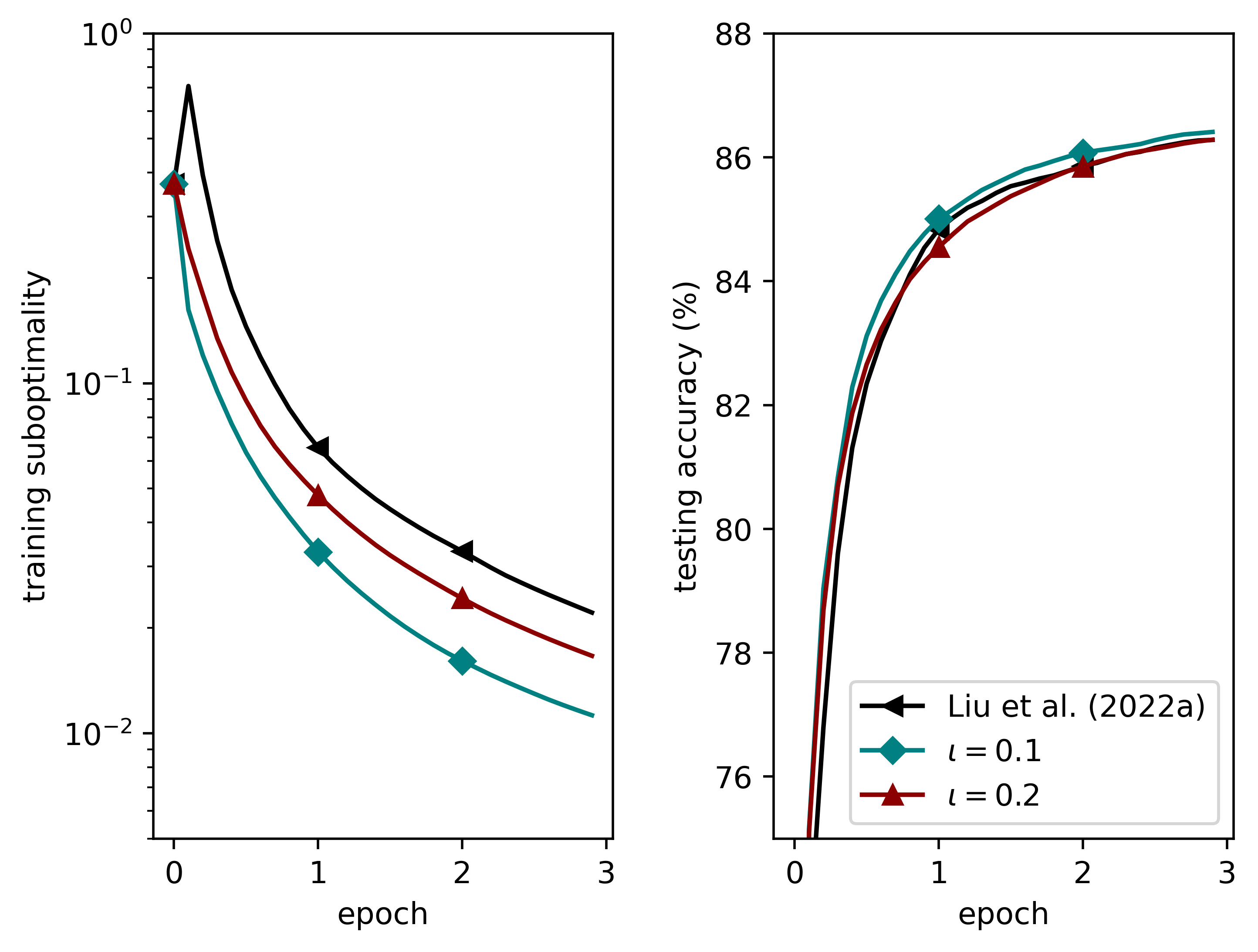
Figure 1: Performance comparison between Algorithm 1 and [19] for $l_{2}$-regularized SVM with $\varepsilon=0.8$.

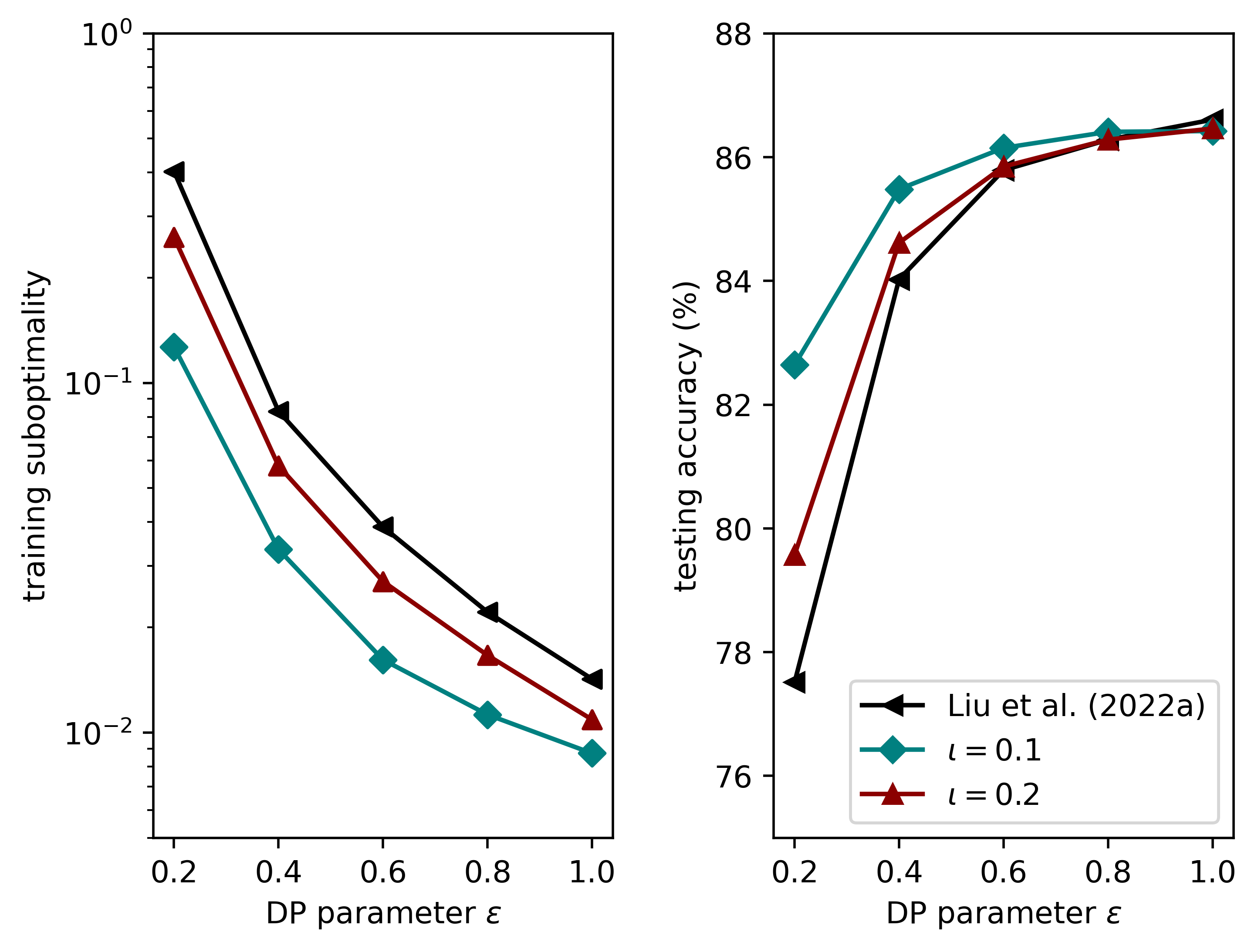
Figure 2: Privacy–utility tradeoff in $l_{2}$-regularized SVM. The suboptimality and accuracy are evaluated after $3$-epoch training.

5.3 Results for $l_{1}$-regularized SVM

Set $h(x)=\phi\lVert x\rVert_{1}$ with $\phi=0.0005$. In this case, the problem in (26) is convex with a non-smooth regularization term. According to Corollary 3.4, we set $\gamma_{t}=0.01\sqrt{t}$ and $a_{t}=1$ in the experiment.

First, we set $\varepsilon=0.4$ and compare Algorithm 1 under different subsampling ratios. The findings depicted in Fig. 3 illustrate a similar trend: As the subsampling ratio $\iota$ decreases, the utility loss diminishes correspondingly. Additionally, we present the results for Algorithm 1 with various DP parameters in Fig. 4. Notably, for both selected subsampling ratios, we observe a degradation in utility as the DP parameter $\varepsilon$ decreases.

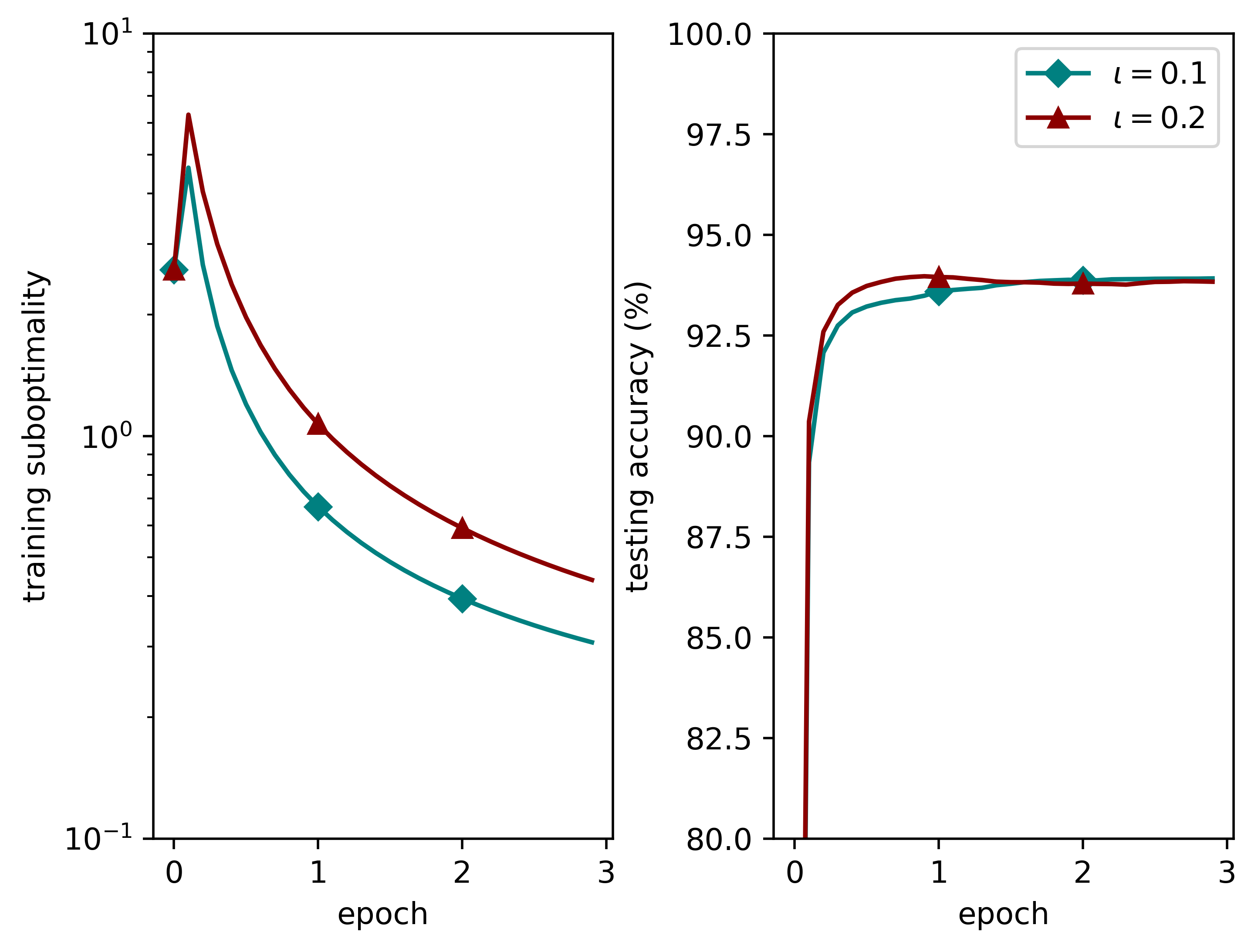
Figure 3: Performance comparison between Algorithm 1 with different $\iota$ for $l_{1}$-regularized SVM with $\varepsilon=0.4$.

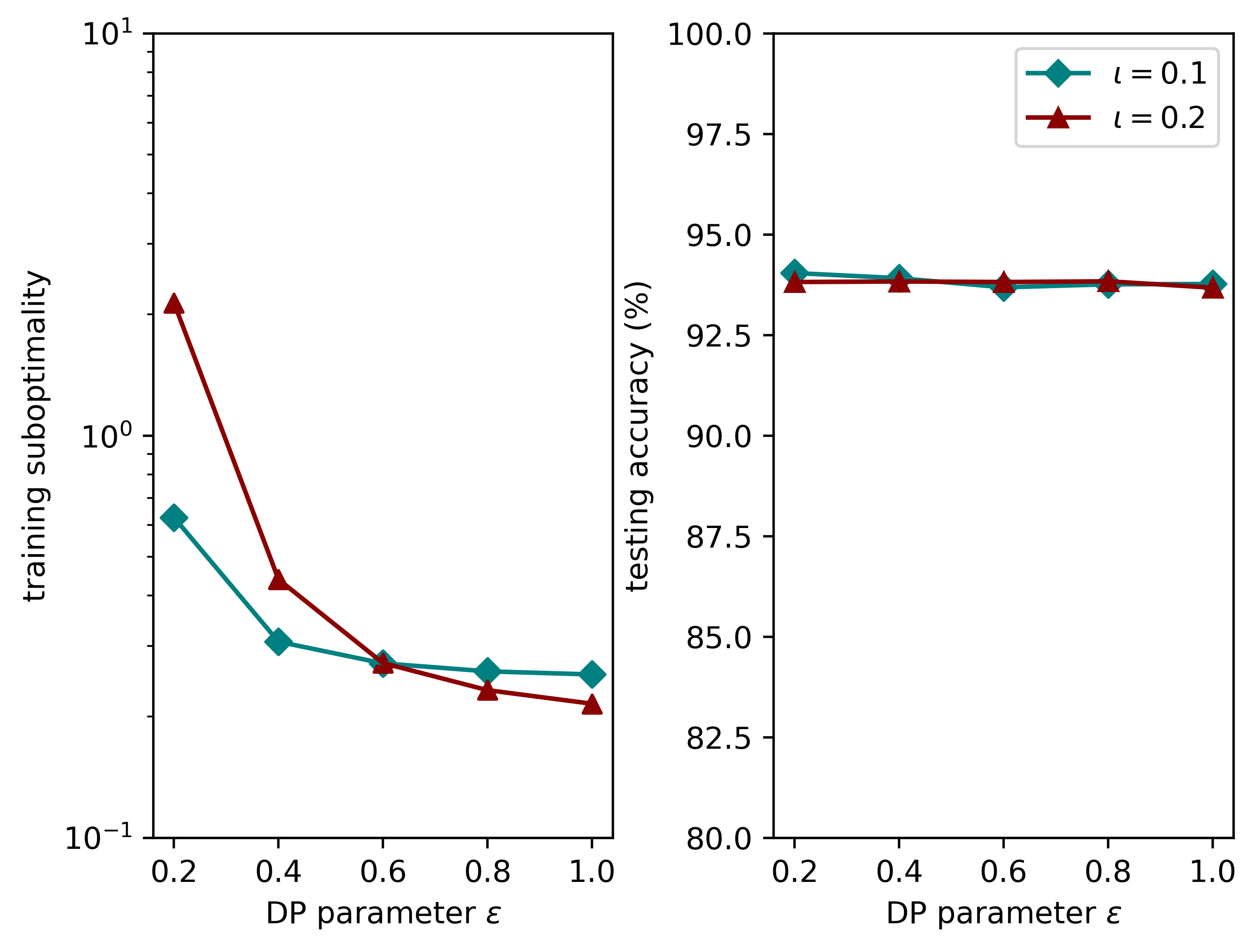
Figure 4: Privacy–utility tradeoff in $l_{1}$-regularized SVM. The suboptimality and accuracy are evaluated after $3$-epoch training.

In summary, the experimental results reveal the effectiveness of the proposed algorithms and validate our theoretical findings.

6 Conclusion

In this work, we presented a class of differentially private DDA algorithms for solving ERM over networks. The proposed algorithms achieve DP by i) randomly activating a fraction of nodes at each time instant and ii) perturbing the stochastic subgradients over individual data samples within activated nodes. We proved that our algorithms substantially improve over existing ones in terms of utility loss.

There are numerous promising directions for future endeavors. Firstly, an intriguing avenue to explore is the heterogeneous case, where nodes exhibit substantial variations in dataset size and/or Lipschitz constants. Secondly, it is worthwhile to investigate the high probability convergence of the proposed algorithms.

Appendix A Proof of Lemma 4.5

Notation: To facilitate the presentation, we introduce the following notation. Define ${\bm{W}}^{(t)}=W^{(t)}\otimes I$. Given a real-valued random vector $x$, we let

$$\lVert x\rVert_{\mathbb{E}}=\sqrt{\mathbb{E}[\lVert x\rVert^{2}]}.$$ (28)

Accordingly, for a square random matrix $W$, we denote $\lVert W\rVert_{\mathbb{E}}=\sup_{\lVert x\rVert_{\mathbb{E}}=1}\lVert Wx\rVert_{\mathbb{E}}$. Denote ${\bf y}^{(t)}={\bf 1}\otimes y^{(t)}$ and

$${\bf z}^{(t)}=\begin{bmatrix}z_{1}^{(t)}\\ \vdots\\ z_{n}^{(t)}\end{bmatrix},{\bf x}^{(t)}=\begin{bmatrix}x_{1}^{(t)}\\ \vdots\\ x_{n}^{(t)}\end{bmatrix},{{\bm{\zeta}}}^{(t)}=\begin{bmatrix}{\zeta}_{1}^{(t)}\\ \vdots\\ {\zeta}_{n}^{(t)}\end{bmatrix},{\bm{\eta}}^{(t)}=\begin{bmatrix}{\eta}_{1}^{(t)}\\ \vdots\\ {\eta}_{n}^{(t)}\end{bmatrix}.$$ (29)

This proof consists of three parts. First, we prove

$$\begin{split}\lVert{\bf x}^{(t)}-{\bf y}^{(t)}\rVert\leq\frac{1}{\gamma_{t}+\mu\iota A_{t}}\left\lVert{\bf z}^{(t)}-{\bm{1}}\otimes\overline{z}^{(t)}\right\rVert,\end{split}$$ (30)

where $\overline{z}(t)=n^{-1}\sum_{i=1}^{n}z_{i}(t)$. Second, we prove

$$\left\lVert\frac{{\bf z}^{(t)}}{a_{t}}-\frac{{\bf 1}\otimes\overline{z}^{(t)}}{a_{t}}\right\rVert^{2}_{\mathbb{E}}\leq\frac{n\iota(L^{2}+m\sigma^{2})}{(1-\beta)^{2}}.$$ (31)

Finally, we conclude the proof using these two inequalities.

Part i) Following [20, Lemma 5], we have $\iota A_{\tau}h(x)+\gamma_{\tau}d(x)$ is $(\mu\iota A_{\tau}+\gamma_{\tau})$-strongly convex, and $\Psi_{\tau}^{*}$, defined by

$$\begin{split}\Psi_{\tau}^{*}(w)=\sup_{{x}}\left\{\langle w,x\rangle-\iota A_{\tau}h(x)-\gamma_{\tau}d(x)\right\},\end{split}$$ (32)

has $(\mu\iota A_{\tau}+\gamma_{\tau})^{-1}$-Lipschitz continuous gradients. Let ${\theta}^{(t)}=n^{-1}\sum_{i=1}^{n}\eta_{i}^{(t)}{\zeta}_{i}^{(t)}$ and $\circ$ be the Hadamard product. Due to

$$\begin{split}&\overline{z}^{(t+1)}=\frac{1}{n}({\bf 1}^{T}\otimes I){\bf z}^{(t+1)}\\ &=\frac{{\bf 1}^{T}\otimes I}{n}{\bm{W}}^{(t)}\left({\bf z}^{(t)}+a_{t}{\bm{\eta}}^{(t)}\circ{\bm{\zeta}}^{(t)}\right)\\ &=\frac{({\bf 1}^{T}\otimes I)}{n}\left({\bf z}^{(t)}+{a_{t}}{\bm{\eta}}^{(t)}\circ{\bm{\zeta}}^{(t)}\right)\\ &=\overline{z}^{(t)}+a_{t}\theta^{(t)},\end{split}$$

we have $y^{(\tau)}=\nabla\Psi_{\tau}^{*}\left(-\sum_{k=1}^{\tau-1}a_{k}\theta^{(k)}\right)=\nabla\Psi_{\tau}^{*}\left(-z^{(t)}\right).$ In addition, $x_{i}^{(\tau)}=\nabla\Psi_{\tau}^{*}(-{z}_{i}^{(\tau)}),\,\forall i=1,\dots,n,$ which gives us (30).

Part ii) When $t=1$, since $z_{i}^{(1)}=0$ for all $i$, we have $\overline{z}^{(1)}=0$ and therefore (31) satisfied. Next, we consider the case with $t\geq 1$.

Let $\tilde{\bf z}^{(t+1)}={\bf z}^{(t+1)}-{\bf 1}\otimes\overline{z}^{(t+1)}$. Then,

$$\begin{split}{\tilde{\bf z}^{(\tau+1)}}=\tilde{\bm{W}}^{(\tau)}\left({\tilde{\bf z}^{(\tau)}}+a_{\tau}\left({\bm{\eta}}^{(\tau)}\circ{\bm{\zeta}}^{(\tau)}-{\bf 1}\otimes\theta^{(\tau)}\right)\right),\end{split}$$ (33)

where $\tilde{\bm{W}}^{(\tau-1)}=\tilde{W}^{(\tau-1)}\otimes I$ and $\tilde{W}^{(\tau-1)}={W}^{(\tau-1)}-\frac{{\bf 1}{\bf 1}^{T}}{n}$. By iterating (33), we obtain

$$\begin{split}&{\tilde{\bf z}^{(t)}}=\sum_{\tau=1}^{t-1}\tilde{\bm{W}}^{(\tau,t-1)}a_{\tau}\left({\bm{\eta}}^{(\tau)}\circ{\bm{\zeta}}^{(\tau)}-{\bf 1}\otimes\theta^{(\tau)}\right)\\ &=\sum_{\tau=1}^{t-1}\tilde{\bm{W}}^{(\tau,t-1)}a_{\tau}\left({\bm{\eta}}^{(\tau)}\circ{\bm{\zeta}}^{(\tau)}\right),\end{split}$$ (34)

where $\tilde{\bm{W}}^{(\tau,t-1)}=\tilde{\bm{W}}^{(t-1)}\dots\tilde{\bm{W}}^{(\tau)}$. Since ${\bf 1}\otimes\theta^{(\tau)}=({\bf 1}\otimes I)\theta^{(\tau)}$ and $(A\otimes B)(C\otimes D)=(AC)\otimes(BD)$, we have $\left(\tilde{W}^{(\tau,t-1)}\otimes I\right)({\bf 1}\otimes\theta^{(\tau)})=\left(\left(\tilde{W}^{(\tau,t-1)}{\bf 1}\right)\otimes I\right)\theta^{(\tau)}=0$. Therefore, (34) can be rewritten as, $\forall t\geq 1$,

$$\begin{split}{\tilde{\bf z}^{(t)}}=\sum_{\tau=1}^{t-1}\tilde{\bm{W}}^{(\tau,t-1)}a_{\tau}\left({\bm{\eta}}^{(\tau)}\circ{\bm{\zeta}}^{(\tau)}\right).\end{split}$$

Upon taking the norm defined in (28) on both sides and using the Minkowski inequality [10], we obtain

$$\begin{split}&\lVert\tilde{\bf{z}}^{(t)}\rVert_{\mathbb{E}}\leq\sum_{\tau=1}^{t-1}a_{\tau}\left\lVert\tilde{\bm{W}}^{(\tau,t-1)}\left({\bm{\eta}}^{(\tau)}\circ{\bm{\zeta}}^{(\tau)}\right)\right\rVert_{\mathbb{E}}.\end{split}$$ (35)

Consider

$$\begin{split}&\left\lVert\tilde{\bm{W}}^{(\tau,t-1)}\left({\bm{\eta}}^{(\tau)}\circ{\bm{\zeta}}^{(\tau)}\right)\right\rVert^{2}_{\mathbb{E}}\\ &\overset{(i)}{=}\mathbb{E}\Big{[}\left({\bm{\eta}}^{(\tau)}\circ{\bm{\zeta}}^{(\tau)}\right)^{T}(\tilde{\bm{W}}^{(\tau,t-2)})^{T}\Big{(}(\tilde{\bm{W}}^{(t-1)})^{T}\tilde{\bm{W}}^{(t-1)}\Big{)}\\ &\quad\quad\,\,\times\tilde{\bm{W}}^{(\tau,t-2)}\left({\bm{\eta}}^{(\tau)}\circ{\bm{\zeta}}^{(\tau)}\right)\Big{]}\\ &\overset{(ii)}{\leq}\left\lVert\tilde{\bm{W}}^{(\tau,t-2)}\left({\bm{\eta}}^{(\tau)}\circ{\bm{\zeta}}^{(\tau)}\right)\right\rVert^{2}_{\mathbb{E}}\rho\left(\mathbb{E}_{W}\left[(\tilde{W}^{(t-1)})^{T}\tilde{W}^{(t-1)}\right]\right)\\ &\overset{(iii)}{\leq}\beta^{2}\left\lVert\tilde{\bm{W}}^{(\tau,t-2)}\left({\bm{\eta}}^{(\tau)}\circ{\bm{\zeta}}^{(\tau)}\right)\right\rVert^{2}_{\mathbb{E}}\\ &\overset{(iv)}{\leq}\beta^{2(t-\tau-1)}\left\lVert\tilde{\bm{W}}^{(\tau)}\left({\bm{\eta}}^{(\tau)}\circ{\bm{\zeta}}^{(\tau)}\right)\right\rVert^{2}_{\mathbb{E}},\end{split}$$

where we use $(A\otimes B)(C\otimes D)=(AC)\otimes(BD)$ and that $\tilde{W}^{(t-1)}$ is independent of the random events that occur up to time $t-2$ to obtain (i) and (ii), respectively, (iii) is due to $\mathbb{E}[(\tilde{W}^{(t-1)})^{T}\tilde{W}^{(t-1)}]=\mathbb{E}[(W^{(t-1)})^{T}W^{(t-1)}]-\frac{{\bf 1}{\bf 1}^{T}}{n}$ and (iv) is by iteration. Therefore, we get from (35) that

$$\begin{split}&\lVert\tilde{\bf{z}}^{(t)}\rVert_{\mathbb{E}}\leq\sum_{\tau=1}^{t-1}\beta^{t-\tau-1}a_{\tau}\left\lVert\tilde{\bm{W}}^{(\tau)}\left({\bm{\eta}}^{(\tau)}\circ{\bm{\zeta}}^{(\tau)}\right)\right\rVert_{\mathbb{E}}\\ &\leq\sum_{\tau=1}^{t-1}\beta^{t-\tau-1}a_{\tau}\left\lVert\tilde{\bm{W}}^{(\tau)}\right\rVert_{\mathbb{E}}\left\lVert{\bm{\eta}}^{(\tau)}\circ{\bm{\zeta}}^{(\tau)}\right\rVert_{\mathbb{E}}\\ &\leq\sum_{\tau=1}^{t-1}\beta^{t-\tau-1}a_{\tau}\left\lVert{\bm{\eta}}^{(\tau)}\circ{\bm{\zeta}}^{(\tau)}\right\rVert_{\mathbb{E}},\end{split}$$

where the last inequality is due to $\left\lVert\tilde{\bm{W}}^{(\tau)}\right\rVert_{\mathbb{E}}\leq 1$, leading to

$$\begin{split}&\lVert\tilde{\bf{z}}^{(t)}\rVert^{2}_{\mathbb{E}}\leq\left(\sum_{\tau=1}^{t-1}a_{\tau}\beta^{t-\tau-1}\left\lVert{\bm{\eta}}^{(\tau)}\circ{\bm{\zeta}}^{(\tau)}\right\rVert_{\mathbb{E}}\right)^{2}\\ &\leq\left(\sum_{\tau=1}^{t-1}\left(\beta^{\frac{t-\tau-1}{2}}\right)^{2}\right)\left(\sum_{\tau=1}^{t-1}\left(a_{\tau}\beta^{\frac{t-\tau}{2}}\left\lVert{\bm{\eta}}^{(\tau)}\circ{\bm{\zeta}}^{(\tau)}\right\rVert_{\mathbb{E}}\right)^{2}\right)\\ &\leq\frac{1}{1-\beta}\sum_{\tau=1}^{t}a_{\tau}^{2}\beta^{t-\tau-1}\left\lVert{\bm{\eta}}^{(\tau)}\circ{\bm{\zeta}}^{(\tau)}\right\rVert^{2}_{\mathbb{E}},\end{split}$$

where the second inequality is due to $(w+v)^{2}\leq 2w^{2}+2v^{2}$. Upon dividing both sides by $a_{t}^{2}$ and using $0<a_{\tau}\leq a_{t},\forall\tau\leq t$, we have

$$\begin{split}&\left\lVert\frac{\tilde{\bf{z}}^{(t)}}{a_{t}}\right\rVert^{2}_{\mathbb{E}}\leq\frac{1}{1-\beta}\sum_{\tau=1}^{t}\frac{a_{\tau}^{2}}{a_{t}^{2}}\beta^{t-\tau-1}\left\lVert{\bm{\eta}}^{(\tau)}\circ{\bm{\zeta}}^{(\tau)}\right\rVert^{2}_{\mathbb{E}}\\ &\leq\frac{n\iota(L^{2}+m\sigma^{2})}{(1-\beta)^{2}}.\end{split}$$

Part iii) Based on (30) and (31), we have

$$\begin{split}\frac{{n}\iota(L^{2}+m\sigma^{2})a_{t}^{2}}{(1-\beta)^{2}(\mu\iota A_{t}+\gamma_{t})^{2}}\geq\lVert{\bf x}^{(t)}-{\bf y}^{(t)}\rVert^{2}_{\mathbb{E}}\geq\sum_{i=1}^{n}\lVert{x}_{i}^{(t)}-{y}^{(t)}\rVert^{2}_{\mathbb{E}}.\end{split}$$

By the Jensen’s inequality, we have

$$\begin{split}\mathbb{E}\left[\lVert{\bf x}^{(t)}-{\bf y}^{(t)}\rVert\right]\leq\sqrt{\lVert{\bf x}^{(t)}-{\bf y}^{(t)}\rVert^{2}_{\mathbb{E}}}\leq\frac{\sqrt{n\iota}(L+\sqrt{m}\sigma)a_{t}}{(\gamma_{t}+\mu\iota A_{t})(1-\beta)}.\end{split}$$

This together with the bound between $l_{1}$ and $l_{2}$-norms, i.e., $\frac{1}{\sqrt{n}}\sum_{i=1}^{n}\lVert x_{i}^{(t)}-y^{(t)}\rVert\leq\lVert{\bf x}^{(t)}-{\bf y}^{(t)}\rVert$ yields

$$\sum_{i=1}^{n}\mathbb{E}[\lVert x_{i}^{(t)}-y^{(t)}\rVert]\leq\frac{{n\iota}(L+\sqrt{m}\sigma)a_{t}}{(\gamma_{t}+\mu\iota A_{t})(1-\beta)}.$$ (36)

This completes the proof.

Appendix B Proof of Lemma 4.6

Recall (32)

$$\begin{split}\Psi_{\tau}^{*}(w)=\sup_{{x}}\left\{\langle w,x\rangle-\iota A_{\tau}h(x)-\gamma_{\tau}d(x):=R_{\tau}(x,w)\right\}.\end{split}$$

Since $-R_{\tau}(\cdot,w)$ is $(\mu\iota A_{\tau}+\gamma_{\tau})$-strongly convex, we have

$$\nabla\Psi_{\tau}^{*}\left(-\sum_{k=1}^{\tau-1}a_{k}{\theta}^{(k)}\right)=y^{(\tau)},$$

where ${\theta}^{(t)}=n^{-1}\sum_{i=1}^{n}\eta_{i}^{(t)}{\zeta}_{i}^{(t)}$, and $\Psi_{{\tau}}^{*}$ has $(\mu\iota A_{\tau}+\gamma_{\tau})^{-1}$-Lipschitz continuous gradients, see, e.g., [20, Lemma 5], implying

$$\begin{split}&\Psi_{{\tau}}^{*}\left(-\sum_{k=1}^{\tau}a_{k}{\theta}^{(k)}\right)\\ &\leq\Psi_{{\tau}}^{*}\left(-\sum_{k=1}^{\tau-1}a_{k}{\theta}^{(k)}\right)-{a_{\tau}}\langle{y}^{(\tau)},{\theta}^{(\tau)}\rangle+\frac{a_{\tau}^{2}\left\lVert{\theta}^{(\tau)}\right\rVert^{2}}{2(\mu\iota A_{\tau}+\gamma_{\tau})}.\end{split}$$ (37)

Upon using $\gamma_{\tau}$ is non-decreasing and $d(x)\geq 0$, we have

$$\begin{split}&\Psi_{{\tau}}^{*}\left(-\sum_{k=1}^{\tau-1}a_{k}{\theta}^{(k)}\right)=R_{\tau}\left(y^{(\tau)},-\sum_{k=1}^{\tau-1}a_{k}{\theta}^{(k)}\right)\\ &=R_{\tau-1}\left(y^{(\tau)},-\sum_{k=1}^{\tau-1}a_{k}{\theta}^{(k)}\right)-\iota a_{\tau}h(y^{(\tau)})\\ &\quad+(\gamma_{\tau-1}-\gamma_{\tau})d(y^{(\tau)})\\ &\leq R_{\tau-1}\left(y^{(\tau)},-\sum_{k=1}^{\tau-1}a_{k}{\theta}^{(k)}\right)-\iota a_{\tau}h(y^{(\tau)})\\ &\leq\Psi_{{\tau-1}}^{*}\left(-\iota\sum_{k=1}^{\tau-1}a_{k}{\theta}^{(k)}\right)-\iota a_{\tau}h(y^{(\tau)}).\end{split}$$ (38)

Upon plugging (38) into (37) and summing up the resultant inequality from $\tau=1$ to $\tau=t$, we have

$$\begin{split}&\sum_{\tau=1}^{t}a_{\tau}\left(\langle{\theta}^{(\tau)},{y}^{(\tau)}\rangle+\iota h(y^{(\tau)})\right)\\ &\leq\Psi_{0}^{*}(0)-\Psi_{\tau}^{*}\left(-\sum_{k=1}^{\tau}a_{k}{\theta}^{(k)}\right)+\sum_{\tau=1}^{t}\frac{a_{\tau}^{2}\lVert{\theta}^{(\tau)}\rVert^{2}}{2(\mu\iota A_{\tau}+\gamma_{\tau})}.\end{split}$$

Note that $y^{(1)}=\nabla\Psi_{{1}}^{*}(0)$, $A_{0}=0$ and $\gamma_{0}=0$ by definition, implying that $\Psi_{0}^{*}(0)=0$. Further considering

$$\begin{split}&\sum_{\tau=1}^{t}a_{\tau}\langle\theta^{(\tau)},-x^{*}\rangle\leq\iota A_{t}h(x^{*})+\gamma_{t}d(x^{*})\\ &\quad+\sup_{x}\left\{-\sum_{k=1}^{\tau}a_{k}\langle\theta^{(k)},x\rangle-\iota A_{t}h(x)-\gamma_{t}d(x)\right\}\\ &\leq\Psi_{t}^{*}\left(-\sum_{k=1}^{\tau}a_{k}\theta^{(k)}\right)+\iota A_{t}h(x^{*})+\gamma_{t}d(x^{*}),\end{split}$$

we obtain

$$\begin{split}&\sum_{\tau=1}^{t}a_{\tau}\Big{(}\langle\theta^{(\tau)},{y}^{(\tau)}-x^{*}\rangle+\iota\left(h(y^{(\tau)})-h(x^{*})\right)\Big{)}\\ &\leq\sum_{\tau=0}^{t}\frac{a_{\tau}^{2}\lVert\theta^{(\tau)}\rVert^{2}}{2(\mu\iota A_{\tau}+\gamma_{\tau})}+\gamma_{t}d(x^{*}).\end{split}$$ (39)

Dividing both sides by $\iota>0$ leads to the desired inequality.

Appendix C Proof of Corollary 3.2

We obtain from the update of $A_{t}$ in Algorithm 1 that

$$\sum_{\tau=1}^{t}\frac{a_{\tau}^{2}}{\mu\iota A_{\tau}+\gamma_{\tau}}=\sum_{\tau=1}^{t}\frac{2\tau^{2}}{\mu\iota\tau(\tau+1)}\leq\frac{2t}{\mu\iota}.$$ (40)

Due to $\mu$-strong convexity of $F$, we have

$$\begin{split}&\sum_{i=1}^{n}\lVert\tilde{x}_{i}^{(t)}-x^{*}\rVert^{2}\leq 2\sum_{i=1}^{n}\lVert\tilde{x}_{i}^{(t)}-\tilde{y}^{(t)}\rVert^{2}+2n\lVert\tilde{y}^{(t)}-x^{*}\rVert^{2}\\ &\leq 2\lVert\tilde{x}_{i}^{(t)}-\tilde{y}^{(t)}\rVert^{2}+\frac{4n}{\mu}\Big{(}F(\tilde{y}^{(t)})-F(x^{*})\Big{)}.\end{split}$$ (41)

Upon using convexity of the $l_{2}$-norm and (19), we obtain

$$\begin{split}&\sum_{i=1}^{n}\mathbb{E}\left[\lVert\tilde{x}_{i}^{(t)}-\tilde{y}^{(t)}\rVert^{2}\right]\leq\mathbb{E}\left[\frac{1}{A_{t}}\sum_{\tau=0}^{t}\sum_{i=1}^{n}a_{\tau}\lVert x_{i}^{(\tau)}-y^{(\tau)}\rVert^{2}\right]\\ &\leq\frac{1}{A_{t}}\sum_{\tau=1}^{t}\frac{a_{\tau}^{3}}{(\mu\iota A_{\tau}+\gamma_{\tau})^{2}}\left(\frac{\iota nL^{2}}{(1-\beta)^{2}}\right)\\ &\leq\frac{4nL^{2}}{\mu^{2}\iota A_{t}(1-\beta)^{2}}\sum_{\tau=1}^{t}\frac{1}{a_{\tau}}\leq\frac{4nL^{2}(\log t+1)}{\mu^{2}\iota A_{t}(1-\beta)^{2}}.\end{split}$$ (42)

By putting expectations on (41) and using (42) and (9), we arrive at (10) as desired.

Appendix D Proof of Corollary 3.4

Under the choices of $a_{t}=1$ and $\gamma_{t}=\gamma\sqrt{t}$, we have

$$\sum_{\tau=1}^{t}\frac{a_{\tau}^{2}}{\mu\iota A_{\tau}+\gamma_{t}}=\frac{1}{\gamma}\sum_{\tau=1}^{t}\frac{1}{\sqrt{\tau}}\leq\frac{2}{\gamma}\sqrt{t}.$$

Therefore, by using (9) and (18), we obtain for all $t\geq 1$,

$$\mathbb{E}\left[F(\tilde{y}^{(t)})-F(x^{*})\right]\leq\frac{d(x^{*})+2\iota M}{\iota\gamma\sqrt{t}}$$

and

$$\frac{1}{n}\sum_{i=1}^{n}\mathbb{E}\left[\lVert x_{i}^{(t)}-y^{(t)}\rVert\right]\leq\frac{L\sqrt{\iota}}{\gamma(1-\beta)\sqrt{t}},\quad i=1,\dots,n$$

respectively. Since $l_{2}$-norm is convex, we have

$$\frac{1}{n}\sum_{i=1}^{n}\mathbb{E}[\lVert\tilde{x}_{i}^{(t)}-\tilde{y}^{(t)}\rVert]\leq\frac{1}{t}\sum_{\tau=1}^{t}\frac{L\sqrt{\iota}}{\gamma(1-\beta)\sqrt{t}}\leq\frac{2L\sqrt{\iota}}{\gamma(1-\beta)\sqrt{t}}.$$ (43)

Appendix E Proof of Corollary 3.5

By (40), we have

$$\begin{split}&\mathbb{E}[F(\tilde{y}^{(T)})-F(x^{*})]\leq\frac{4M}{\mu\iota(T+1)}+\frac{80m\log(2/\delta_{0})\iota^{2}L^{2}}{\mu q^{2}\varepsilon^{2}}\\ &\quad\quad\quad\quad\quad\quad\quad\quad\quad\quad+\frac{16\sqrt{10m\log(2/\delta_{0})\iota}L^{2}}{\mu q\varepsilon(1-\beta)\sqrt{T+1}},\end{split}$$

where $M$ is a positive constant defined in Theorem 2. Similar to (42), we have

$$\begin{split}\frac{1}{n}\sum_{i=1}^{n}\mathbb{E}\left[\lVert\tilde{x}_{i}^{(T)}-\tilde{y}^{(T)}\rVert^{2}\right]\leq\frac{8(L^{2}+m\sigma^{2})(\log T+1)}{\mu^{2}\iota T(T+1)(1-\beta)^{2}}.\end{split}$$

Following (41), we set $T=\mathcal{O}\left(\frac{q^{2}\varepsilon^{2}}{\iota^{3}(1-\beta)^{2}m\log(1/\delta_{0})}\right)$ to obtain (13).

Appendix F Proof of Corollary 3.6

By the specific choices of parameters in (14), we obtain from (9) that

$$\begin{split}&\mathbb{E}[F(\tilde{y}^{(T)})-F(x^{*})]\\ &\leq\frac{d(x^{*})+2\iota M}{\gamma\iota\sqrt{T}}+\frac{40m\iota^{3}L^{2}\log(2/\delta_{0})}{\gamma{q^{2}}\varepsilon^{2}}\sum_{t=1}^{T}\frac{1}{\sqrt{t}}\\ &\quad+\frac{4\sqrt{10m\iota\log(2/\delta_{0})}\iota L^{2}}{\gamma q\varepsilon(1-\beta)\sqrt{T}}\sum_{t=1}^{T}\frac{1}{\sqrt{t}}\\ &\leq\frac{d(x^{*})+2\iota M}{\gamma\iota\sqrt{T}}+\frac{8\sqrt{10m\iota\log(2/\delta_{0})}\iota L^{2}}{\gamma q\varepsilon(1-\beta)}\\ &\quad+\frac{80m\iota^{3}L^{2}\log(2/\delta_{0})\sqrt{T}}{{\gamma}{q^{2}}\varepsilon^{2}},\end{split}$$

where the last inequality is due to $\sum_{t=1}^{T}\frac{1}{\sqrt{t}}\leq 1+\int_{1}^{T}\frac{1}{\sqrt{t}}dt\leq 2\sqrt{t}.$ Upon using $\iota\leq 1-\beta$ and $T=\mathcal{O}\left(\frac{q^{2}\varepsilon^{2}}{\iota^{3}(1-\beta)^{2}{m\log(1/\delta_{0})}}\right)$, we arrive at (15). In addition, similar to (43), we have

$$\begin{split}&\frac{1}{n}\sum_{i=1}^{n}\mathbb{E}[\lVert\tilde{x}_{i}^{(T)}-\tilde{y}^{(T)}\rVert]\\ &\leq\frac{2(L+\sqrt{m}\sigma)\sqrt{\iota}}{\gamma(1-\beta)\sqrt{T}}\leq\mathcal{O}\left(\frac{L\sqrt{m\iota\log(1/\delta_{0})}}{\gamma q\varepsilon}\right).\end{split}$$

References

- [1] Martin Abadi, Andy Chu, Ian Goodfellow, H Brendan McMahan, Ilya Mironov, Kunal Talwar, and Li Zhang. Deep learning with differential privacy. In Proceedings of the 2016 ACM SIGSAC Conference on Computer and Communications Security, pages 308–318, 2016.
- [2] Raef Bassily, Adam Smith, and Abhradeep Thakurta. Private empirical risk minimization: Efficient algorithms and tight error bounds. In 2014 IEEE 55th Annual Symposium on Foundations of Computer Science, pages 464–473. IEEE, 2014.
- [3] Kamalika Chaudhuri, Anand Sarwate, and Kaushik Sinha. Near-optimal differentially private principal components. Advances in Neural Information Processing Systems, 25:989–997, 2012.
- [4] Fei Chen, Xiaozheng Chen, Linying Xiang, and Wei Ren. Distributed economic dispatch via a predictive scheme: heterogeneous delays and privacy preservation. Automatica, 123:109356, 2021.
- [5] Igor Colin, Aurélien Bellet, Joseph Salmon, and Stéphan Clémençon. Gossip dual averaging for decentralized optimization of pairwise functions. In International Conference on Machine Learning, pages 1388–1396. PMLR, 2016.
- [6] Tie Ding, Shanying Zhu, Jianping He, Cailian Chen, and Xinping Guan. Differentially private distributed optimization via state and direction perturbation in multiagent systems. IEEE Transactions on Automatic Control, 67(2):722–737, 2021.
- [7] John C Duchi, Alekh Agarwal, and Martin J Wainwright. Dual averaging for distributed optimization: Convergence analysis and network scaling. IEEE Transactions on Automatic Control, 57(3):592–606, 2011.
- [8] Cynthia Dwork. Differential privacy. In International Colloquium on Automata, Languages, and Programming, pages 1–12. Springer, 2006.
- [9] Antonious M Girgis, Deepesh Data, Suhas Diggavi, Peter Kairouz, and Ananda Theertha Suresh. Shuffled model of federated learning: Privacy, accuracy and communication trade-offs. IEEE Journal on Selected Areas in Information Theory, 2(1):464–478, 2021.
- [10] Allan Gut. Probability: A Graduate Course, volume 75. Springer Science & Business Media, 2013.
- [11] Dongyu Han, Kun Liu, Yeming Lin, and Yuanqing Xia. Differentially private distributed online learning over time-varying digraphs via dual averaging. International Journal of Robust and Nonlinear Control, 32(5):2485–2499, 2022.
- [12] Shuo Han, Ufuk Topcu, and George J Pappas. Differentially private distributed constrained optimization. IEEE Transactions on Automatic Control, 62(1):50–64, 2016.
- [13] Rui Hu, Yuanxiong Guo, Hongning Li, Qingqi Pei, and Yanmin Gong. Personalized federated learning with differential privacy. IEEE Internet of Things Journal, 7(10):9530–9539, 2020.
- [14] Zhenqi Huang, Sayan Mitra, and Nitin Vaidya. Differentially private distributed optimization. In Proceedings of the 2015 International Conference on Distributed Computing and Networking, pages 1–10, 2015.
- [15] Peter Kairouz, Sewoong Oh, and Pramod Viswanath. The composition theorem for differential privacy. In International Conference on Machine Learning, pages 1376–1385. PMLR, 2015.
- [16] Daniel Kifer, Adam Smith, and Abhradeep Thakurta. Private convex empirical risk minimization and high-dimensional regression. In Proceedings of the 25th Annual Conference on Learning Theory, volume 23, pages 25.1–25.40. PMLR, 2012.
- [17] David D Lewis, Yiming Yang, Tony Russell-Rose, and Fan Li. RCV1: A new benchmark collection for text categorization research. Journal of Machine Learning Research, 5:361–397, 2004.
- [18] Xiangru Lian, Ce Zhang, Huan Zhang, Cho-Jui Hsieh, Wei Zhang, and Ji Liu. Can decentralized algorithms outperform centralized algorithms? a case study for decentralized parallel stochastic gradient descent. In Advances in Neural Information Processing Systems, pages 5330–5340, 2017.
- [19] Changxin Liu, Karl H. Johansson, and Yang Shi. Private stochastic dual averaging for decentralized empirical risk minimization. IFAC-PapersOnLine, 55(13):43–48, 2022.
- [20] Changxin Liu, Zirui Zhou, Jian Pei, Yong Zhang, and Yang Shi. Decentralized composite optimization in stochastic networks: A dual averaging approach with linear convergence. IEEE Transactions on Automatic Control, 2022.
- [21] Haihao Lu, Robert M Freund, and Yurii Nesterov. Relatively smooth convex optimization by first-order methods, and applications. SIAM Journal on Optimization, 28(1):333–354, 2018.
- [22] Luca Melis, Congzheng Song, Emiliano De Cristofaro, and Vitaly Shmatikov. Exploiting unintended feature leakage in collaborative learning. In 2019 IEEE Symposium on Security and Privacy (SP), pages 691–706. IEEE, 2019.
- [23] Angelia Nedic and Asuman Ozdaglar. Distributed subgradient methods for multi-agent optimization. IEEE Transactions on Automatic Control, 54(1):48–61, 2009.
- [24] Maxence Noble, Aurélien Bellet, and Aymeric Dieuleveut. Differentially private federated learning on heterogeneous data. In International Conference on Artificial Intelligence and Statistics, pages 10110–10145. PMLR, 2022.
- [25] F. Pedregosa, G. Varoquaux, A. Gramfort, V. Michel, B. Thirion, O. Grisel, M. Blondel, P. Prettenhofer, R. Weiss, V. Dubourg, J. Vanderplas, A. Passos, D. Cournapeau, M. Brucher, M. Perrot, and E. Duchesnay. Scikit-learn: Machine learning in Python. Journal of Machine Learning Research, 12:2825–2830, 2011.
- [26] Sören Sonnenburg, Gunnar Rätsch, Christin Schäfer, and Bernhard Schölkopf. Large scale multiple kernel learning. Journal of Machine Learning Research, 7:1531–1565, 2006.
- [27] Wei Tao, Wei Li, Zhisong Pan, and Qing Tao. Gradient descent averaging and primal-dual averaging for strongly convex optimization. In Proceedings of the AAAI Conference on Artificial Intelligence, volume 35, pages 9843–9850, 2021.
- [28] Stefan Vlaski and Ali H Sayed. Graph-homomorphic perturbations for private decentralized learning. In ICASSP 2021-2021 IEEE International Conference on Acoustics, Speech and Signal Processing (ICASSP), pages 5240–5244. IEEE, 2021.
- [29] Di Wang, Minwei Ye, and Jinhui Xu. Differentially private empirical risk minimization revisited: faster and more general. In Proceedings of the 31st International Conference on Neural Information Processing Systems, pages 2719–2728, 2017.
- [30] Jimin Wang, Ji-Feng Zhang, and Xingkang He. Differentially private distributed algorithms for stochastic aggregative games. Automatica, 142:110440, 2022.
- [31] Yongqiang Wang and Angelia Nedić. Tailoring gradient methods for differentially-private distributed optimization. IEEE Transactions on Automatic Control, 2023.
- [32] Hanshen Xiao and Srinivas Devadas. Towards understanding practical randomness beyond noise: Differential privacy and mixup. Cryptology ePrint Archive, 2021.
- [33] Lin Xiao, Stephen Boyd, and Seung-Jean Kim. Distributed average consensus with least-mean-square deviation. Journal of Parallel and Distributed Computing, 67(1):33–46, 2007.
- [34] Yongyang Xiong, Jinming Xu, Keyou You, Jianxing Liu, and Ligang Wu. Privacy-preserving distributed online optimization over unbalanced digraphs via subgradient rescaling. IEEE Transactions on Control of Network Systems, 7(3):1366–1378, 2020.
- [35] Jie Xu, Wei Zhang, and Fei Wang. : Asynchronous decentralized parallel stochastic gradient descent with differential privacy. IEEE Transactions on Pattern Analysis and Machine Intelligence, 2021.
- [36] Deming Yuan, Yiguang Hong, Daniel WC Ho, and Guoping Jiang. Optimal distributed stochastic mirror descent for strongly convex optimization. Automatica, 90:196–203, 2018.
- [37] Chunlei Zhang, Muaz Ahmad, and Yongqiang Wang. ADMM based privacy-preserving decentralized optimization. IEEE Transactions on Information Forensics and Security, 14(3):565–580, 2018.
- [38] Hongyi Zhang, Moustapha Cisse, Yann N Dauphin, and David Lopez-Paz. mixup: Beyond empirical risk minimization. In International Conference on Learning Representations, 2018.
- [39] Jiaqi Zhang, Kai Zheng, Wenlong Mou, and Liwei Wang. Efficient private ERM for smooth objectives. In Proceedings of the 26th International Joint Conference on Artificial Intelligence, pages 3922–3928, 2017.
- [40] Tao Zhang and Quanyan Zhu. Dynamic differential privacy for ADMM-based distributed classification learning. IEEE Transactions on Information Forensics and Security, 12(1):172–187, 2016.
- [41] Xueru Zhang, Mohammad Mahdi Khalili, and Mingyan Liu. Improving the privacy and accuracy of ADMM-based distributed algorithms. In International Conference on Machine Learning, pages 5796–5805. PMLR, 2018.
- [42] Junlong Zhu, Changqiao Xu, Jianfeng Guan, and Dapeng Oliver Wu. Differentially private distributed online algorithms over time-varying directed networks. IEEE Transactions on Signal and Information Processing over Networks, 4(1):4–17, 2018.
- [43] Ligeng Zhu and Song Han. Deep leakage from gradients. In Federated Learning, pages 17–31. Springer, 2020.