The spectrum of QCD with one flavour: A Window for Supersymmetric Dynamics

Abstract

We compute the spectrum of the low-lying mesonic states with vector, scalar and pseudoscalar quantum numbers in QCD with one flavour. With three colours the fundamental and the two-index anti-symmetric representations of the gauge group coincide. The latter is an orientifold theory that maps into the bosonic sector of $\mathcal{N}=1$ super Yang-Mills theory in the large number of colours limit.

We employ Wilson fermions along with tree-level improvement in the gluonic and fermionic parts of the action. In this setup the Dirac operator can develop real negative eigenvalues. We therefore perform a detailed study in order to identify configurations where the fermion determinant is negative and eventually reweight them. We finally compare results with effective field theory predictions valid in the large $N_{C}$ limit and find reasonably consistent values despite $N_{C}$ being only three. Additionally, the spin-one sector provides a novel window for supersymmetric dynamics.

I Introduction

Understanding the dynamics of strongly coupled gauge theories, such as QCD, has motivated the construction of several expansions complementary to the standard, perturbative, weak coupling expansion. One of the most prominent examples is the large $N_{C}$ limit (where $N_{C}$ is the number of colours), introduced by ’t Hooft in Ref. ’t Hooft (1974). In this case one keeps quarks in the fundamental representation of the gauge group $SU(N_{C})$ and organises an expansion in $1/N_{C}$ using a diagrammatic approach. Several properties of QCD can then be understood in a simple way, suggesting that $N_{C}=3$ is “large”. However, since quark loops are suppressed in this expansion, the properties of the $\eta^{\prime}$-meson are not well reproduced in the ’t Hooft large $N_{C}$ limit. Baryons also become increasingly heavy as $N_{C}$ grows.

Partly motivated by that, Corrigan and Ramond (CR) introduced a different large $N_{C}$ expansion in Ref. Corrigan and Ramond (1979), in which quarks transform according to the two-index antisymmetric representation of the gauge group. While ’t Hooft and CR expansions coincide for $N_{C}=3$, they are very different in the large $N_{C}$ limit. Notably, in the CR expansion, quark loops are not suppressed as $N_{C}\to\infty$. A simple scaling of the dimensionality of the representations of the quark fields suggests that the CR large $N_{C}$ limit may share non-trivial dynamical properties with supersymmetric theories. This relation has been made precise by Armoni, Shifman and Veneziano in Refs. Armoni et al. (2003a, b), where a connection between the mesonic sectors of the two-index (anti-)symmetric theories and of $\mathcal{N}=1$ super Yang-Mills theory (sYM) is established. The subtle issues of the confinement properties and (in)equivalences at large $N_{C}$ were investigated in Ref. Sannino (2005). Further developing the correspondence, in Ref. Sannino and Shifman (2004) supersymmetry inspired effective Lagrangians have been constructed for gauge theories featuring one Dirac fermion transforming either in the symmetric or in the anti-symmetric two-index representation of the gauge group $SU(N_{C})$ (orientifold theories). At leading order in the $1/N_{C}$ expansion such effective theories coincide with that of supersymmetric gluodynamics restricted to its mesonic sector. These correspondences imply that non-perturbative quantities computed in orientifold theories can be related, up to $1/N_{C}$ effects, to the analogous ones in sYM. By considering $1/N_{C}$ supersymmetry breaking effects, including the explicit ones due to a finite quark mass, a number of predictions are made in Ref. Sannino and Shifman (2004) concerning the spectrum of the low-lying mesonic states. In this work we confront such predictions with non-perturbative results produced by means of lattice simulations. For simplicity, in this first study we only consider $N_{C}=3$, which corresponds to one-flavour QCD. This has the advantage that available simulation packages for lattice QCD can be used without having to develop new code for handling representations of the fermionic fields different from the fundamental one. Future studies will be devoted to the extension to $N_{C}>3$. Intriguingly, by flipping the point of view (cf. Refs. Sannino (2005); Feo et al. (2004)), we can use QCD results to learn about the spectrum and dynamics of supersymmetric theories, in particular $\mathcal{N}=1$ sYM. Analytic and numerical studies can now be employed to investigate several dynamical properties, including the theta-angle Sannino and Shifman (2004).

One-flavour QCD has been the object of several previous lattice studies. The qualitative behaviour of the theory has been discussed in Ref. Creutz (2007). In Ref. DeGrand et al. (2006) the quark condensate has been computed by comparing the density of low-lying eigenvalues of the overlap Dirac operator to predictions from Random Matrix Theory Leutwyler and Smilga (1992); Shuryak and Verbaarschot (1993). The result is consistent with the prediction for the gluino condensate in sYM obtained in Ref. Armoni et al. (2004). Using Wilson fermions, Ref. Farchioni et al. (2007) presents a computation of the low-lying hadronic spectrum of one-flavour QCD. We improve here on that computation by considering a finer lattice spacing, larger volumes and a tree-level improved fermionic action. In Ref. Francis et al. (2018) the one-flavour $SU(2)$ vector gauge theory with the fermion in the fundamental representation is studied as a possible composite model for Dark Matter (DM). The Dirac operator is discretised using Wilson’s regularisation. The fundamental representation of $SU(2)$ is pseudo-real making the global symmetries and dynamics different from three colours QCD. In particular, the dark-matter model of Ref. Francis et al. (2018) features a mass-gap with vector mesons being the lightest triplet of the enhanced $SU(2)$ global symmetry. A similar DM model based on $SU(2)$ gauge theory with scalar quarks was proposed in Ref. Hambye and Tytgat (2010).

Finally, in Ref. Athenodorou et al. (2021) the single flavour $SU(2)$ theory is considered with the fermion in the adjoint representation. The goal in this case is to gain insights on the emergence of the conformal window. Again the Wilson Dirac operator is used in the numerical simulations. As is highlighted by this brief review, one-flavour QCD is implemented on the lattice by adopting either overlap (or more generally Ginsparg-Wilson) or Wilson fermions. That is because in those cases the single-flavour lattice Dirac operator can be rigorously defined. Wilson fermions are computationally cheaper but in such regularisation the spectrum of the Dirac operator may contain real negative eigenvalues for positive (but small) quark masses. That might cause a sign problem as the fermion determinant may become negative on some configurations. Following Refs. Edwards et al. (1998a, b); Akemann et al. (2011); Mohler and Schaefer (2020) we discuss in detail how we monitor such cases.

Earlier numerical investigations of orientifold theories Lucini et al. (2010); Armoni et al. (2008) used the quenched approximation where the sign problem is absent.

Directly simulating supersymmetric gauge theories on the lattice has been an active research field for many years. Since the literature is vast we refer the reader to the recent review in Ref. Schaich (2023) and references within for a discussion of the status and open problems.

A preliminary account of the results we present in this paper appeared in Refs. Ziegler et al. (2022); Della Morte et al. (2022). The latter in particular contains some algorithmic exploratory studies for $N_{C}=4,5$ and $6$.

The remainder of this paper is organised as follows. In Section II we describe our computational setup and provide algorithmic details. In Section III we investigate the consequences of the sign problem in our simulations. In Section IV we report on the correlation function fits required to extract the spectrum at non-zero quark masses, before extrapolating the meson spectrum to vanishing quark masses in Sec. V. Finally, in Section VI we confront the effective field theory predictions with our results and provide an outlook.

II Simulation setup

For the gauge part of the action, we employ the Symanzik improved gauge action Iwasaki (1983) with a fixed value for the gauge coupling of $\beta=4.5$. As fermion action we use one flavour of tree-level improved Wilson fermions Sheikholeslami and Wohlert (1985) and set the parameter of the clover term to 1. The Wilson-Dirac operator $D$ in clover improved form is defined as follows

$$D(m_{0})= \frac{1}{2}\sum_{\nu=0}^{3}\left(\gamma_{\nu}(\nabla_{\nu}^{*}+\nabla_{\nu})-a\nabla_{\nu}^{*}\nabla_{\nu}\right)$$

$$+\ ac_{\mathrm{SW}}\sum_{\nu,\rho=0}^{3}\frac{i}{4}\sigma_{\nu\rho}\hat{F}_{\nu\rho}+m_{0}\,,$$ (1)

where $a$ is the lattice spacing, $m_{0}$ is the bare quark mass and $\nabla_{\nu}^{(*)}$ denotes the covariant forward (backward) derivative. The hopping parameter $\kappa$ is related to the bare mass $m_{0}$ by $1/\kappa~{}=~{}2(am_{0}+4)$.

$L/a$	$\kappa$	ML steps	$\tau_{MD}$	$\Delta\text{cfg}$ [MDU]	$N_{\text{config}}$	Acceptance
12	0.1350	1,1,6	2.0	64	877	0.998
12	0.1370	1,1,6	2.0	64	778	0.997
12	0.1390	1,1,6	2.0	64	731	0.996
12	0.1400	1,1,6	2.0	64	674	0.996
16	0.1350	1,1,8	3.0	120	1512	0.999
16	0.1370	1,1,8	3.0	120	539	0.998
16	0.1390	1,1,8	3.0	120	1189	0.997
16	0.1400	1,1,8	3.0	120	959	0.994
16	0.1405	1,1,8	3.0	120	686	0.991
16	0.1410	1,1,10	3.0	120	989	0.957
20	0.1350	1,1,6	2.0	64	503	0.996
20	0.1370	1,1,6	2.0	64	180	0.993
20	0.1390	1,1,8	3.0	120	346	0.993
24	0.1350	1,1,10	2.0	64	360	0.999
24	0.1390	1,1,6	2.0	64	324	0.986
24	0.1405	1,1,6	2.0	64	286	0.966
24	0.1410	1,1,9	2.0	64	593	0.841
32	0.1390	1,1,6	2.0	64	180	0.979
32	0.1400	1,1,6	2.0	64	376	0.967

Table 1: Overview of the lattice ensembles generated in this study. All configurations are at a fixed gauge coupling of $\beta=4.5$ and a fixed temporal extent of $T/a=64$. The simulation parameters were tuned to achieve a high acceptance with a large trajectory length $\tau_{MD}$. We refer the reader to the text for the definitions of the parameters.

In order to map out the relevant parameter space we generated 19 gauge field ensembles covering different hopping parameters $\kappa$ between 0.1350 and 0.1410 and volumes ranging from $12^{3}\times 64$ to $32^{3}\times 64$. An overview of the simulation parameters can be found in Table 1.

We measure the topological charge $Q$ by integrating the Wilson flow Lüscher (2010) using a third-order Runge-Kutta scheme with a step-size of $\epsilon=0.01$ and $1600$ integration steps. The topological charge at the largest flow time ($t/a^{2}=16$) is shown for all ensembles in Fig. 19 in Appendix A. The topological charge behaves as expected: its distribution is narrower for lighter quark masses and broader for larger volumes Leutwyler and Smilga (1992). The Wilson flow further allows us to estimate the lattice spacing (via the reference flow scale $t_{0}$) by studying the Yang-Mills gauge action density as a function of flow-time Lüscher (2010). Since our goal is to determine dimensionless quantities, we only quote the lattice spacing in order to enable qualitative comparison with other lattice calculations. As there is no reference scale for a single flavour ($N_{f}=1$), we use the average of $t_{0}$ from $N_{f}=0$ Lüscher (2010) and $N_{f}=2$ Bruno and Sommer (2014) as an estimate for the lattice spacing with $N_{f}=1$. In practice, we use a value of $\sqrt{8t_{0}}=0.45\,$fm. This allows us to obtain an indicative value for the lattice spacing of $a\approx 0.06\,$fm.

All configurations are generated using the openQCD software package Lüscher, M. and Schäfer, S. . Since we only simulate a single fermion in the sea, it is necessary to use the rational hybrid Monte Carlo (RHMC) algorithm Clark and Kennedy (2007). In the rational approximation we adopt a Zolotarev functional of degree 10. In the absence of prior knowledge about the optimal Zolotarev approximation – in particular for just one flavour – we choose a conservative range of $0.002$ and $9.0$ as a lower and upper bound for the position of the poles. In comparison with Ref. Mohler and Schaefer (2020) this is a rather loose approximation, which is relevant for the tunnelling between regions of configuration space with positive and negative determinants of the Dirac operator. In addition, we include frequency splitting, i.e. we factorise the Zolotarev rational into two terms, where the first factor contains the poles $1$ to $5$ and the second term the contribution from poles $6$ to $10$. Throughout the entire generation, we adopt three levels of integration schemes. The outermost employs a second-order Omelyan integrator I.P. Omelyan and I.M. Mryglod and R. Folk (2003) with $\lambda=1/6$, which is used for the contributions from poles $6$ to $10$. For the inner two levels we use fourth-order Omelyan integrators, where the remaining fermion force is calculated in the second, and the gauge forces in the innermost level. We tune the number of fermion integration steps (ML steps) in the different levels to achieve a high acceptance (between $84\%$ and $99.9\%$, c.f. Table 1). The pseudofermion actions and forces are obtained using a simple multi-shift conjugate gradient solver. For ensembles with a lighter quark mass, i.e. with larger values of $\kappa$, we take advantage of the deflated SAP Luscher (2007a, b) preconditioned solver given in the openQCD framework. The trajectory lengths of our ensembles are typically between 2 and 3 molecular dynamic (MD) units. In our analysis, we use every 32nd (or 40th) trajectory, which implies that configurations are at least 64 MD units apart from each other. For each ensemble the resulting number of configurations $N_{\mathrm{config}}$ on which we perform all measurements is listed in Table 1. To increase the amount of statistics and to utilise smaller computing resources more efficiently, we branch our simulation stream into multiple replicas after thermalisation is reached.

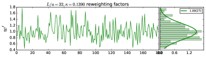
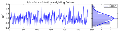
Figure 1: Normalised reweighting factors on two example ensemble.

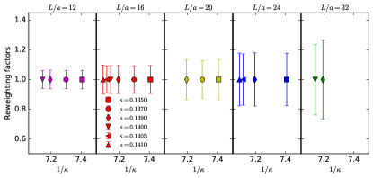
Figure 2: Typical spread of normalised reweighting factors as a function of volume and quark mass.

Since the Zolotarev approximation in the RHMC is not exact, we correct our observables by using a reweighting scheme. To achieve this, on each configuration we compute four estimators for the reweighting factors $w_{i}$ using code from the openQCD package. The correctly reweighted gauge average of an observable $O$ is then given by

$$\left<O\right>_{\mathrm{rew}}=\frac{\left<wO\right>}{\left<w\right>}=\left<w^{\prime}O\right>\,,$$ (2)

where we define $w^{\prime}=w/\left<w\right>$. Figure 1 shows these normalised reweighting factors $w^{\prime}$ as a function of the trajectory length (excluding any thermalisation times) for two representative ensembles ($L/a=32$, $\kappa=0.1390$ and $L/a=24$, $\kappa=0.1405$). In Fig. 2 we show the variation of the reweighting factors for all ensembles and observe that the fluctuations increase with volume, but are insensitive to the quark mass.

As the phase space of this theory in the regularisation we have chosen is a priori unknown, we computed the trace of the Polyakov loop. We find that the Polyakov loop vanishes within errors on each ensemble, which indicates that we are simulating in the confined phase.

III Eigenvalue analysis

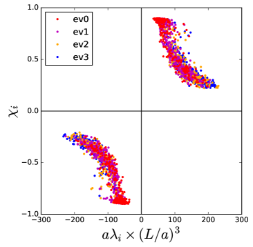
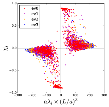
Figure 3: Scatter plot of the lowest four eigenvalues and chiralities for $L/a=16$ and $\kappa=0.1405$ (left) and $\kappa=0.1410$ (right).

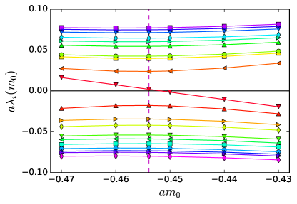
Figure 4: Tracking analysis of the lowest 20 eigenvalues on a $L/a=16$, $\kappa=0.1410$ configuration with a negative fermion determinant.

The use of Wilson fermions for lattice QCD with an odd number of quark flavours or with non-mass-degenerate (light) quarks can introduce a sign problem. This occurs because the configuration space is divided into two sectors, one associated to a positive sign of the fermion determinant and one to a negative sign. These sectors are separated by a zero of the fermionic measure. Note that the latter translates into a pole of the fermionic force in the molecular dynamics algorithm. With exact integration and an exact expression for the square root function, the negative sector cannot be reached from the positive one. In practice the algorithmic choices for the rational approximation yield a finite (rather than infinite) barrier between the two sectors.

In the thermodynamic and continuum limit the trajectory is expected to be constrained to the positive sector. However, at finite volume, the presence of the negative sector has to be accounted for by sign reweighting which requires knowledge of the sign of the fermion determinant $\det(D)$. A direct computation is numerically (prohibitively) expensive. Instead we follow a strategy in which the sign of $\det(D)$ is inferred from computing a few of the lowest eigenvalues of the Dirac operator. This can be achieved at a cost linear in the lattice volume and using the approach we will now sketch:

Due to $\gamma_{5}$-Hermiticity of the Wilson-Dirac operator, i.e.

$$D^{\dagger}=\gamma_{5}D\gamma_{5}\,,$$ (3)

the matrix $Q=\gamma_{5}D$ is Hermitian and its spectrum is real. Furthermore, it holds that $\det(D)=\det(\gamma_{5})\det(D)=\det(Q)$ and that a zero eigenvalue of $D$ is also a zero eigenvalue of $Q$. Recalling that the eigenvalues of $D$ come in complex conjugate pairs, for $\det(D)$ to be negative there must be an odd number of negative real eigenvalues of $D$.

Since the fermion determinant $\det(D)$ is assumed to be positive for large quark masses, we can infer that the determinant at the unitary mass $m_{0}^{*}$, used in the actual simulation, is negative if and only if there is an odd number of eigenvalues that cross zero as the mass is decreased from large quark masses to $m_{0}^{*}$. The idea is to locate (on each gauge configuration) the largest value $m_{t}$ of the quark mass such that $Q(m_{t})$, and therefore $D(m_{t})$, has a zero eigenvalue. If $m_{0}^{*}$ is larger than this value $m_{t}$ then $D(m_{0}^{*})=D(m_{t})+(m_{0}^{*}-m_{t})I$ has no negative eigenvalues. Conversely, if $m_{0}^{*}<m_{t}$, we need to determine the number of zero crossings of the lowest eigenvalue(s) $\lambda(m_{0})$ of $Q(m_{0})$ by varying the bare mass $m_{0}$ from above $m_{t}$ down to $m_{0}^{*}$. To that end we combine the PRIMME package with openQCD as mentioned in Ref. Mohler and Schaefer (2020).

In practice we proceed in two steps: First we perform a preselection to identify potential candidate configurations with a negative fermion determinant and for this subset of configurations we perform a tracking analysis to identify the configurations that indeed display a negative fermion determinant.

We start the preselection by measuring the lowest O(10) eigenpairs $(\lambda_{i},\psi_{i})(m_{0}^{*})$ and their chiralities $\chi_{i}(m_{0}^{*})$, defined by

$$\chi_{i}(m_{0}^{*})=\left<\psi_{i}\vphantom{\gamma_{5}\psi_{i}}\right|\left.\gamma_{5}\psi_{i}\vphantom{\psi_{i}}\right>(m_{0}^{*})=\left.\frac{d\lambda_{i}(m_{0})}{dm_{0}}\right|_{m_{0}=m_{0}^{*}}\,,$$ (4)

where the last equality follows from the Feynman-Hellman theorem Akemann et al. (2011); Mohler and Schaefer (2020). The chirality hence corresponds to the slope of the eigenvalue function. This allows to categorise the eigenvalues of $Q$ into those which approach zero as $m_{0}$ is increased and those which move away from it. In Figure 3 we plot the results of the eigenvalue-chirality analysis for the four lowest lying eigenvalues of the two $L/a=16$ ensembles with $\kappa=0.1405$ (left) and $\kappa=0.1410$ (right). If a datapoint falls into the north-east or south-west quadrant, the eigenvalue moves further away from zero when the quark mass is increased, implying that there is no zero crossing for values larger than $m_{0}^{*}$. This is the case for all configurations with $\kappa=0.1405$. Conversely, if a datapoint falls into the north-west or south-east quadrant this implies that the eigenvalue approaches zero as the quark mass is increased and a zero crossing is possible. Configurations with eigenvalues which display this feature can potentially have a negative determinant and therefore require further monitoring. As can be seen in Fig. 3, on the $\kappa=0.1410$ ensembles we find a small number of these cases for which the second step, the tracking analysis, is performed.

We find that datapoints close to the horizontal axis but in the “safe” quadrants, tend to occur only for comparably large values of $\left|\lambda\right|$. Under the assumption that the chirality changes slowly in the range of masses explored, even if the sign of $\chi$ were to change, the corresponding eigenvalues are not expected to be at risk of changing sign. This assumption is justified a posteriori in the tracking analysis.

On the configurations that displayed datapoints in the north-west or south-east quadrants we now measure the lowest 20 eigenpairs for several partially quenched masses around $m_{0}^{*}$. The eigenvalue functions $\lambda_{i}(m_{0})$ and the eigenbasis $\{\psi_{i}\}$ are assumed to vary slowly and continuously with $m_{0}$. Assuming that the different partially quenched masses are sufficiently close to each other it is possible to track how a particular eigenvalue behaves as a function of the quark mass as follows. For each set of neighbouring masses $m_{0}$ and $m_{0}+\Delta m_{0}$ we construct the matrix $M_{ij}=\left<\psi_{i}(m_{0})\vphantom{\psi_{j}(m_{0}+\Delta m_{0})}\right|\left.\psi_{j}(m_{0}+\Delta m_{0})\vphantom{\psi_{i}(m_{0})}\right>$ of scalar products between the $i$th eigenvector $\psi_{i}(m_{0})$ at $m_{0}$ and the $j$th eigenvector $\psi_{j}(m_{0}+\Delta m_{0})$ at $m_{0}+\Delta m_{0}$. We determine the largest entry $M_{ij}$ and interpret this to mean that the eigenvalue $i$ at $m_{0}$ evolves to be the eigenvalue $j$ at $m_{0}+\Delta m_{0}$. We then remove row $i$ and column $j$ from the matrix and iterate the procedure until each eigenpair at $m_{0}$ has been assigned a corresponding eigenpair at $m_{0}+\Delta m_{0}$. Figure 4 displays a configuration of the $L/a=16$ and $\kappa=0.1410$ ensemble where a negative determinant was detected. We observe that the line connecting the red downward facing triangles does cross zero as the mass $m_{0}$ is increased from $m_{0}^{*}$ (highlighted as the vertical dashed line). Since there is only a single eigenvalue crossing zero in the region $m_{0}>m_{0}^{*}$, we conclude that the fermion determinant is negative on this particular configuration.

We see from the representative example shown in Figure 4 that the assumption discussed above is indeed valid and the derivatives of the eigenvalues change very little in the range of masses explored. We also see that such derivatives are either of $O(1)$ or small. This is expected and in agreement with the discussion in Ref. Itoh et al. (1987), where approximate relations are derived between the eigenpairs corresponding to small eigenvalues of $Q$ and those of $D$. The chiralities are expected to be significantly different from zero (and in that case close to $\pm 1$) only for eigenvectors corresponding to almost real eigenvalues of $D$.

We performed the above analysis for the two smallest values of the quark mass corresponding to $\kappa=0.1405$ and $0.1410$ for which we each have a $L/a=16$ and a $L/a=24$ ensemble. As discussed above (cf. left panel in Fig. 3) we did not observe any cases of a negative determinant for $\kappa=0.1405$ on either of the two available volumes. Since negative eigenvalues are expected to have a higher likelihood to occur at small quark masses, we did not perform this analysis for any of the remaining larger masses. At $\kappa=0.1410$ we found 6 configurations with a negative determinant for each of the two volumes. Furthermore, we observed that the negative sector is visited at most for the Monte Carlo time corresponding to two consecutive measurements. This might be related to our choice of parameters for the rational approximation of $\sqrt{D^{\dagger}D}$ yielding a relatively low barrier between the two sectors. We conclude that in our computational setup the sign problem for $N_{f}=1$ QCD is mild and the relative frequency of a negative determinant of the Dirac matrix is at the sub-percent level.

IV Correlator analysis

In order to obtain the spectrum of one-flavour QCD, we create mesonic correlation functions for states with a variety of quantum numbers. We are particularly interested in states with scalar (S), pseudoscalar (P) and vector (I) quantum numbers. We employ the Laplacian Heaviside (LapH) method Morningstar et al. (2011); Peardon et al. (2009) which allows us to efficiently compute quark-line disconnected contributions that appear in the computation of mesonic quantities with a single flavour.

IV.1 Construction of correlation functions

Following Ref. Morningstar et al. (2011) and, where possible, using the same notation we compute the $N_{v}$ lowest eigenpairs $(\lambda_{i},v_{i})$ of the three-dimensional gauge-covariant Laplacian using a stout smeared gauge field. On each time slice $t$ we arrange these eigenvectors into a matrix $V_{s}$ as

$$V_{s}(t)=\left(v_{1},v_{2},\cdots,v_{N_{v}}\right)$$ (5)

from which we then define the Hermitian smearing matrix as a function of the number of eigenpairs that were computed as

$$\mathcal{S}(N_{v},t)=V_{s}(t)V_{s}^{\dagger}(t).$$ (6)

Using a low number of eigenpairs corresponds to a broad smearing profile, whereas using a large number of eigenpairs corresponds to “less” smearing and taking the limit of all eigenpairs recovers the identity. Quark lines $\mathcal{Q}$ are computed as

$$\mathcal{Q}(t_{0},t) =\mathcal{S}(t)(\gamma_{4}D)^{-1}\mathcal{S}(t_{0})$$ (7)

$$=V_{s}(t)\left[V_{s}^{\dagger}(t)(\gamma_{4}D)^{-1}V_{s}(t_{0})\right]V_{s}^{\dagger}(t_{0}).$$

The inversion $(\gamma_{4}D)^{-1}V_{s}(t_{0})$ is done by solving the equation

$$(\gamma_{4}D)_{\alpha\beta}(t_{0},t)y^{i}_{\beta}(t)=v_{i}(t_{0})$$ (8)

for $y^{i}_{\beta}(t)$. This is done for each eigenvector $v_{i}$ ($i=1,\ldots,N_{v}$), each spin component ($\alpha=1,\ldots,4$) and each time slice ($t_{0}=0,\ldots,T-1$), amounting to $N_{t}\times N_{v}\times 4$ inversions per configuration.

In our simulation, we keep the number of eigenvalues $N_{v}=20$ fixed for all ensembles. However, from these inversions we can construct operators which use fewer than $20$ eigenvalues by truncating the elements of the square matrix $V_{s}^{\dagger}(t)(\gamma_{4}D)^{-1}V_{s}(t_{0})$. Using this we compute meson correlation functions for $N_{v}\in\{1,2,3,4,5,6,7,8,9,10,12,15,17,20\}$, which describe the same spectrum but have different smearing functions.

In all three channels (P, S, I), we use the appropriate interpolation operator ($\mathcal{P}$, $\mathcal{S}$, $\mathcal{I}$) in the finite volume irreducible representation. For the S–channel we additionally construct a purely gluonic operator $\mathcal{G}$ Brett et al. (2020) which induces the same quantum numbers as the $\mathcal{S}$ operator. We consider all mutual combinations of $\mathcal{G}$ and $\mathcal{S}$ in the ’scalar-glue’ system.

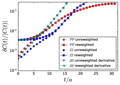
Figure 5: Impact of the reweighting on the relative uncertainties of the correlation functions.

IV.2 Reweighting and vacuum expectation value subtraction

The vacuum subtracted correlation function $C_{\mathcal{X}\mathcal{Y}}$ can be derived from the un-subtracted correlation function $C^{\mathrm{raw}}_{\mathcal{X}\mathcal{Y}}(t)$ and the vacuum expectation values (vevs) $v_{\mathcal{X}}$ and $v_{\mathcal{Y}}$ as

$$C_{\mathcal{X}\mathcal{Y}}(t)=\left<C^{\mathrm{raw}}_{\mathcal{X}\mathcal{Y}}(t)\right>-\left<v_{\mathcal{X}}\right>\left<v_{\mathcal{Y}}\right>\,,$$ (9)

where $\left<\cdot\right>$ denotes the gauge average. Whilst the vev is exactly zero for the $\mathcal{P}$ operator and numerically zero for the $\mathcal{I}$ operator, it is sizable for the $\mathcal{S}$ and $\mathcal{G}$ operators. We find that the statistical signal for correlation functions including $\mathcal{G}$ or $\mathcal{S}$ deteriorates when reweighting (cf. Sec. II) is combined with the naive vacuum expectation value subtraction defined in Eq. (9).

This is due to the fact that the product of the vevs is many orders of magnitude larger than the exponentially decaying part of the correlator and as a consequence even the little noise introduced by the reweighting factors destroys the signal for the latter almost completely.

Since the vacuum expectation value is time-independent, an alternative way to perform the vev subtraction is to take the temporal derivative of the un-subtracted correlation function. We find that this results in a significantly better signal when combined with reweighting and are therefore utilising this.

Figure 5 displays the effect of reweighting for the example of the $N_{v}=20$ correlation functions on the $L/a=20$, $\kappa=0.1390$ ensemble. The figure shows the relative uncertainties of the correlation function for the $\mathcal{PP}$ (red), $\mathcal{II}$ (blue) and the time derivative of the $\mathcal{SS}$ (cyan) operators. The dotted lines connect the un-reweighted data points, whilst the solid lines connect the reweighted ones. We observe that only for the earliest time slices the uncertainty of the reweighted data is limited by the accuracy of the reweighting factors.

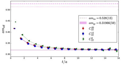
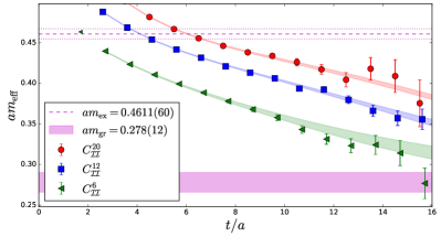
Figure 6: Example fit for the vector two point function for the $L/a=32$, $\kappa=0.1400$ (top) and the $L/a=16$, $\kappa=0.1390$ (bottom) ensembles. The datapoints show the effective masses of the underlying correlation functions, whilst the correspondingly coloured bands show the effective mass obtained from the results of the correlation function fits. Finally the magenta horizontal band (dashed line) show the results for the extracted ground (excited) state energies.

IV.3 Correlation function fits

For a given channel (P, I or S), the correlation function $C$ of operators $O_{\mathcal{X}}^{n}$ with $\mathcal{X}\in\{\mathcal{S},\mathcal{P},\mathcal{I},\mathcal{G}\}$ using $n$ eigenvalues can be approximated by the first $N$ states $X_{i}$ as

$$C^{n}_{\mathcal{X}\mathcal{Y}}(t) =\sum_{i=0}^{N}\left|(Z_{\mathcal{X}}^{n})^{*}_{i}(Z_{\mathcal{Y}}^{n})_{i}\right|\frac{e^{-m^{X}_{i}t}+e^{-m^{X}_{i}(T-t)}}{2m^{X}_{i}}\,,$$ (10)

where $(Z_{\mathcal{X}}^{n})_{i}=\left<X_{i}\vphantom{(O_{\mathcal{X}}^{n})^{\dagger}0}\right|(O_{\mathcal{X}}^{n})^{\dagger}\left|0\vphantom{X_{i}(O_{\mathcal{X}}^{n})^{\dagger}}\right>$. We emphasise that the induced masses $m^{X}_{i}$ depend on the channel $X$, rather than the specific operator $\mathcal{X}$, in particular all combinations of $\mathcal{S},\mathcal{G}$ induce the same spectrum $m_{i}^{S}$.

We extract the three lowest–lying states of the spectrum by performing simultaneous correlated fits to the symmetrised correlation functions $C_{\mathcal{X}\mathcal{Y}}^{n}(t)$ for several choices of $n$ (between 2 and 4). We illustrate two such fits for the example of the vector channel in Fig. 6. We defer the discussion on the slow approach to the ground state for the bottom panel to Sec. V.2. In order to assess systematic uncertainties associated with the choice of smearing radii, we vary which $n$ enter into a particular fit. In particular, for the vector and pseudoscalar channels we perform three different fits, simultaneously fitting $N_{v}=(20,12,6),(17,10,3)$ or $(20,15,10,5)$ and labelled ‘fit1’, ‘fit2’ and ‘fit3’, respectively. For the scalar-glue basis we simultaneously fit $N_{v}=(20,3)$ or $N_{v}=(17,5)$ (‘fit1’ and ‘fit2’) but jointly fitting $C_{\mathcal{S}\mathcal{S}}$, $C_{\mathcal{S}\mathcal{G}}$ and $C_{\mathcal{G}\mathcal{G}}$. In all cases, we fit three states ($N=2$ in (10)), but only the lowest two potentially enter any subsequent analysis. We list the numerical results for the lowest two states (’gr’ and ’ex’, respectively) in Table 2 in Appendix B. In all further steps of the analysis we consider all choices of ‘fit1’, ‘fit2’ and ‘fit3’ to propagate any systematic uncertainties.

Finally, we also compute the connected correlation function for the pseudoscalar meson, which corresponds to a non-existent state in a $N_{f}=1$ theory and in the following is therefore referred to as “fake pion”. As we will discuss in the following section, $m_{\pi}^{\mathrm{fake}}\to 0$ can be used as a proxy for the massless limit (see also Ref. Francis et al. (2018)). These correlation functions are generated from standard point sources and follow the same functional form as Eq. (10) with the replacement $Z_{\mathcal{X}}^{n}\to\left<\pi\vphantom{(\bar{q}\gamma_{5}q)^{\dagger}0}\right|(\bar{q}\gamma_{5}q)^{\dagger}\left|0\vphantom{\pi(\bar{q}\gamma_{5}q)^{\dagger}}\right>$. For these states we perform fits with $N=0$ and $N=1$. We note that for both $\kappa=0.1410$ ensembles we expect large finite size effects as $m_{\pi}^{\mathrm{fake}}L<3$ and therefore discard them from the subsequent analysis.

V Analysis of the spectrum

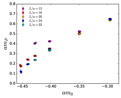
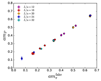
Figure 7: The spectrum of the pseudoscalar meson as a function of the bare quark mass (left) and as a function of the fake pion mass (right). Here and in the following, shown triplets (or pairs) of points correspond to the fit results of ‘fit1’, ‘fit2’, ‘fit3’, respectively.

The goal of this section it so extrapolate the results for the meson spectrum ($m_{P}$, $m_{I}$ and $m_{S}$) to the chiral and infinite volume limit to provide results for ratios of these masses.

V.1 Defining the chiral limit

We start by determining what the best proxy for the quark mass is. Figure 7 shows the lowest lying state for the pseudoscalar channel. The left panel displays this as a function of the bare quark mass, the right panel as a function of the fake pion mass. By comparing the two panels, it is evident that the fake pion mass is the more suitable choice to define the massless limit as the bare quark mass suffers from large finite volume effects. Those are due to discretisation effects in the computation of the critical parameter $\kappa_{c}$ entering the definition of the bare subtracted  quark mass (see Ref. Sommer et al. (2004) for a discussion in the case of QCD). In addition, in Ref. Francis et al. (2018) it has been numerically shown, for the one-flavour $SU(2)$ gauge theory, that the definition of the massless point from the vanishing of the fake pion mass is consistent with the rigorous definition from the continuum relation between the topological susceptibility and the quark mass. In the following we therefore choose the fake pion mass to define the massless limit.

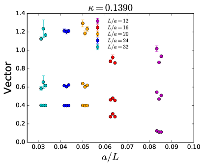
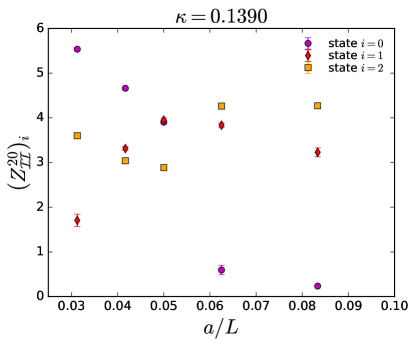
Figure 8: Volume dependence of the vector meson at fixed $\kappa=0.1390$. The top panel shows the dependence of the spectrum, the bottom panel the dependence of the corresponding matrix elements for the $N=20$ correlation function.

V.2 Assignment of states

To understand the behaviour of the spectrum we induced by means of our chosen interpolating fields, we investigate how the hadron masses vary as a function of quark mass and volume. We are predominantly interested in mesonic states dominated by $q\bar{q}$ contributions. These are expected to display a strong quark mass dependence but at most a mild dependence on the volume, whereas any glueball state should only depend weakly on quark mass and volume. Contrary to these, states that depend mildly on the quark mass but strongly on the volume do not correspond to physical states and might be interpreted to be torelon states Michael (1987); Michael and Perantonis (1992).

In Section V.1 we noted that the pseudoscalar mass is largely volume independent, but depends smoothly and strongly on the quark mass set by $m_{\pi}^{\mathrm{fake}}$. We therefore identify this with the desired $q\bar{q}$-state. In the case of the scalar and vector channels, the situation is more complicated. When comparing results of simulations at the same $\kappa$ but on different volumes, there are cases that display significant volume dependence on smaller volumes.

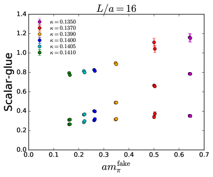
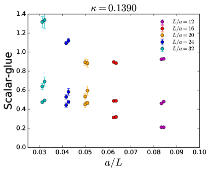
Figure 9: The spectrum of the scalar meson as a function of the quark mass at fixed volume $L/a=16$ (top) and as a function of the volume at fixed $\kappa=0.1390$ (bottom).

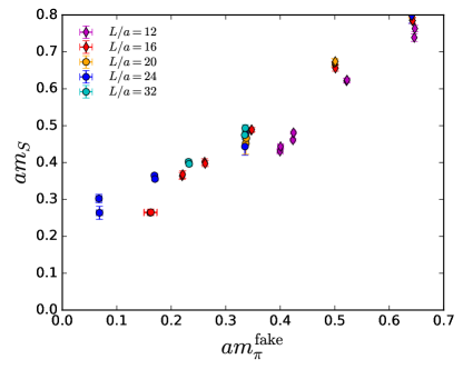
Figure 10: Mass dependence of the states identified as $q\bar{q}$ states for the vector (top) and the scalar (bottom).

For example, the top panel of Figure 8 shows the spectrum as a function of the inverse spatial volume but at fixed $\kappa=0.1390$. We observe that the three largest volumes yield very consistent ground state masses. Contrary, for the two smallest volumes, we see that a lighter state is present in the spectrum, which displays a strong volume dependence. We note that the first excited state on these two volumes is numerically close to the ground state mass extracted on the larger volumes. This picture is further substantiated by investigating the behaviour of the amplitude for the matrix element as we will illustrate with the example of $(Z_{\mathcal{I}}^{20})_{i}$: In the bottom panel of Figure 8 we show these values for the three states we are fitting. For the three largest volumes, which are displaying a consistent ground state mass, we find that the ground state matrix element (left three magenta circles) is of similar size or larger than the other matrix elements. In contrast to this, for the smallest two volumes the situation is reversed and we find the matrix element of the lowest lying state (right two magenta circles) to be significantly smaller than that of the first and second excited states. We further note that for these two smallest volumes, the matrix element corresponding to the first excited state (rightmost two red diamonds) shows a qualitatively similar behaviour to that of the ground state for the larger volumes. In other words, for the smallest two volumes, the correlation function couples more strongly to the first excited state than the ground state. This is also the reason for the slow approach to the plateau for example in the case of the $L/a=16$ and $\kappa=0.1390$ ensemble (c.f. bottom panel of Fig. 6). The strong volume dependence and qualitatively different behaviour with respect to the matrix element indicate that the lowest lying state for the small volumes is not the $q\bar{q}$-state we are interested in. Instead, as indicated by the values of the mass and the amplitudes we identify the first excited state with the $q\bar{q}$ state. In summary, for the vector channel at fixed $\kappa=0.1390$, the $q\bar{q}$ state corresponds to the lowest lying state for $L/a=32,24,20$ and to the first excited state for $L/a=16,12$. Corresponding analyses for the other quark masses yield a similar picture.

Figure 9 addresses the scalar channel. The top panel shows the mass dependence at fixed volume $L/a=16$. The lowest lying state is mass independent in the range of masses we simulate, but the first excited state displays a strong mass dependence. The bottom panel shows the volume dependence at fixed $\kappa=0.1390$. Again, for small volumes, we find a state whose energy increases as the volume increases (lowest state at $L/a=12,16$), as well as a volume insensitive state (lowest state at $L/a=32,24,20$ and first excited state at $L/a=16,12$). Furthermore, the latter coincides with the state that displayed the strong mass dependence in the top panel. In analogy with the discussion of the vector meson, we conclude that those correspond to a (mass dependent, volume independent) scalar meson state and a (mass independent, volume dependent) torelon state.

By means of similar investigations of the volume and quark mass dependence, we categorise the two lowest lying states on each ensemble and in each channel into the lowest quark mass dependent state ($q\bar{q}$) and the remaining state, which in principle can be a torelon, an excited $q\bar{q}$ or a glueball state. Figure 10 shows the state that has been identified as the relevant $q\bar{q}$ state for the vector (top) and scalar (bottom) channels. For the large volumes, good agreement is found for all quark masses, whereas for light quark masses and small volumes finite size effects are sizable. We therefore exclude the $L/a=12$ and $L/a=16$ from our subsequent analysis.

Summarising the discussion in this Section, the $q\bar{q}$ states we are interested in are easily identified at large volumes and small quark masses as the lowest lying states in the respective channels. Such determinations have the largest impact in the chiral and infinite volume extrapolations we discuss next. However, especially for small volumes, the identification required a more detailed study of the volume and mass dependence of both the energy levels and the overlap factors describing the correlation functions. Those are important lessons we will take into account for future studies at large values of $N_{C}$.

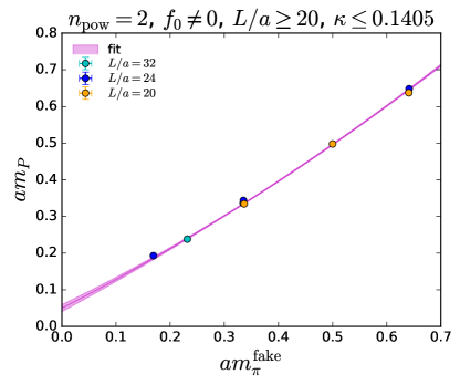
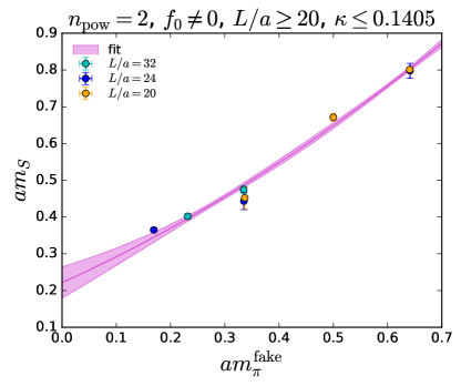
Figure 11: Extrapolation to the chiral limit for a given fit ansatz for the pseudoscalar mass (top) and the scalar mass (bottom).

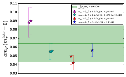
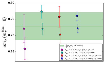
Figure 12: Comparison of the fit results when varying the correlator fit choice and the fit ansatz for the pseudoscalar (top) and the scalar mass (bottom).

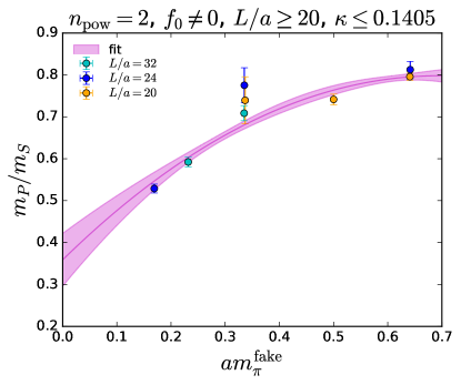
Figure 13: Example extrapolation to the chiral limit of the ratio of pseudoscalar to scalar mass via method 1.

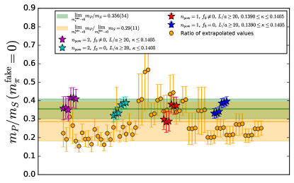
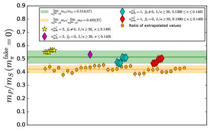
Figure 14: Comparison of fit results for different choices of the extrapolation of the ratio of $m_{P}/m_{S}$. The left plot shows the extrapolation results including even and odd powers in $m_{\pi}^{\mathrm{fake}}$ the right plot for only even powers.

V.3 Extrapolation to zero quark mass

We are interested in the spectrum at vanishing quark mass. Since we have not performed a scale setting analysis we focus on ratios of masses in the chiral limit. As discussed above, we will use the fake pion mass to define the zero quark mass limit. A completely model independent fit function would have to include even and odd powers of the fake pion mass. To give a rigorous definition of the fake pion correlator one would have to consider a partially quenched theory constructed by introducing a quark field with the same mass parameter as the original one and quenching it away by a corresponding ghost field Della Morte and Juttner (2010). Such a theory would be invariant (at zero quark mass) under transformations in an extended (graded) chiral symmetry group. Depending on whether the symmetry is realised à la Wigner-Weyl or à la Nambu-Goldstone, one would obtain different relations between the fake pion mass and the quark mass. In the second case (where the symmetry is broken spontaneously by the vacuum and explicitly by the quark mass) the quark mass would turn out to be proportional to the fake pion mass squared. In this case a fit in terms of only even powers of the fake pion mass would be more appropriate.

Any such Gell-Mann-Oakes-Renner-like Gell-Mann et al. (1968) relation is valid at low energies or very close to the massless limit and in the same limit the fake pion and the pseudoscalar masses should differ significantly, as the first is expected to vanish while the second not. Since in our data we only see small differences between such masses we cannot claim with confidence to be in the regime where such relations apply. We hence favour the more general fit function including even and odd powers of the fake pion mass for our final results.

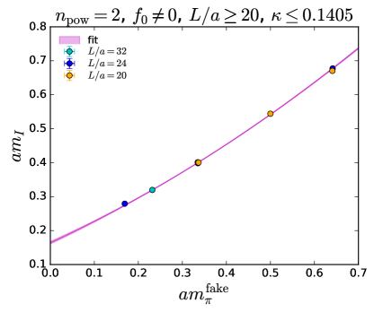
Figure 15: Extrapolation of the vector mass to the chiral limit, analogous to Fig. 11 for different choices.

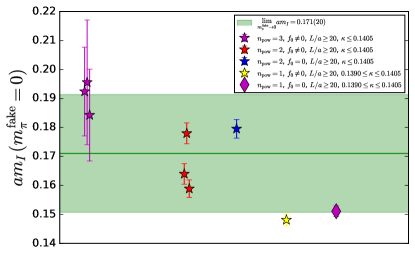
Figure 16: Variations of the extrapolation of the vector mass to the chiral limit, analogous to Fig. 12.

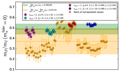
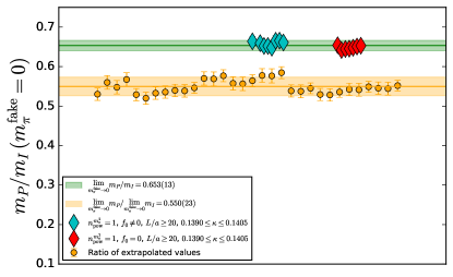
Figure 17: Variations of the extrapolation of the ratio of the pseudoscalar and the vector mass using even and odd powers of $m_{\pi}^{\mathrm{fake}}$ (top) and only even powers of $m_{\pi}^{\mathrm{fake}}$ (bottom).

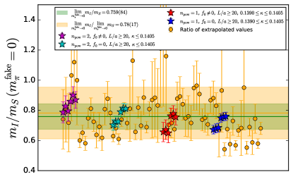
Figure 18: Results of fits to the ratio of the vector and the scalar mass.

The fit functions we explore for this extrapolation are

$$M(m_{\pi}^{\mathrm{fake}},L)=\left[\sum_{i=0}^{\mathrm{n_{\mathrm{pow}}}}c_{i}\left(m^{\mathrm{fake}}_{\pi}\right)^{i}\right]\left(1+f_{0}e^{-m_{P}L}\right)\,,$$ (11)

where $M$ is either a mass ($m_{P}$, $m_{S}$, $m_{I}$) or ratios thereof. In line with what we discussed above, we separately consider choices where $i$ takes even and odd values or only even values and in both cases either leaving $f_{0}$ as a free parameter or setting it to zero. In addition to varying the fit function, we consider cuts to the data, in particular removing the smallest volumes and/or the lightest and/or heaviest masses.

An example fit for the case of the pseudoscalar mass (top) and the scalar mass (bottom) is shown in Figure 11. In both of these cases we take the results obtained by ‘fit1’, keep $f_{0}$ as a free parameter and choose $n_{\mathrm{pow}}=2$. Due to concerns about the finite volume effects, we exclude the smallest volumes ($L/a=12,16$) and the lightest quark mass ($\kappa=0.1410$).

We repeat all extrapolations for the various choices of the correlation function fits, whether or not $f_{0}$ is kept as a free parameter and for different choices of $n_{\mathrm{pow}}$. For the lowest order polynomial we restrict the mass range that enters the fit. The datapoints in Fig. 12 show the results for these variations for the pseudoscalar (top) and the scalar (bottom). Only fits with an acceptable $p$-value of $p>0.05$ are shown. The green band in these plots is derived by taking the 68th percentile of the distribution of the underlying bootstrap samples of all the fits which produced an acceptable $p$-value. We interpret this number to be a good approximation of systematic effects due to correlator fit choices, variations of the chiral fit ansatz and the data included in such a fit.

Ultimately we are interested in the ratio of masses in the chiral limit. We can obtain this in two ways as we will now illustrate on the example of the ratio of the pseudoscalar to the scalar mass: We can either build the ratio $m_{P}/m_{S}$ at finite $m_{\pi}^{\mathrm{fake}}$ and then extrapolate this to the massless limit (method 1), or we can separately extrapolate the pseudoscalar and the scalar masses and then build their ratio (method 2). One example fit of the former is shown in Fig. 13. We observe that part of the mass dependence cancels in the ratios, resulting in a less steep curve than that observed in the individual fits (cf. Fig 11). The coloured stars in the left panel of Fig. 14 show different variations of the fit ansatz, analogous to Fig. 12. In addition to the extrapolation of the ratio of masses (method 1), we also show ratios of the chirally extrapolated values (orange circles; method 2). Here we computed all mutual combinations of acceptable fits displayed in Fig. 12. The green (orange) band is the result of taking the 68th percentile of all the bootstrap samples for the fits of method 1 (method 2) that produced an acceptable $p$-value.

In general, we notice that the ratio of separate chiral extrapolations leads to larger variations than the extrapolation of the ratio of masses. This is unsurprising as, ensemble by ensemble, the underlying datapoints are statistically correlated, and therefore statistical fluctuations are reduced for the individual ratios of datapoints. Furthermore the extrapolation of the individual datapoints is more difficult to control since the slope with the fake pion mass is steeper. Our preferred number is therefore the direct extrapolation (green band in Fig. 14) whilst the orange band provides a sanity check.

We are now in a position to compare the results of the fits including even and odd powers of $m_{\pi}^{\mathrm{fake}}$ to those only using even powers. These two choices are compared in the two panels of Fig. 14 for the example of the ratio of pseudoscalar to scalar masses. The green bands of the two panels are in $\sim 2\sigma$ agreement, lending confidence in the results. However the errorbands of the direct and indirect methods do not overlap for the fit of the even powers only. This is even more pronounced for the case of the ratio $m_{P}/m_{I}$ (c.f. the bottom panel of Fig 17). This numerical evidence further supports our preference for the more conservative fit ansatz including even and odd powers of $m_{\pi}^{\mathrm{fake}}$ and we therefore quote results from this choice as our final numbers.

In addition to $m_{P}$, $m_{S}$ we have data for the vector mass $m_{I}$. An example fit for the extrapolation of the vector mass is shown in Fig. 15 (cf. Fig. 11) whilst different fit variations are shown in Fig. 16 (cf. Fig. 12). Finally, we also construct the ratios $m_{P}/m_{I}$ (see Fig. 17) and $m_{I}/m_{S}$ (see Fig. 18) in the chiral limit via the two methods described above.

VI Discussion and Outlook

We have presented a detailed study of the spectrum of one-flavour QCD using Wilson fermions with tree-level O$(a)$ improvement.

Results are obtained at one single lattice spacing (approximatively $0.06$ fm) for different volumes (up to $32^{3}\times 64$) and several quark masses. After extrapolating to the massless limit we obtain

$$\frac{m_{P}}{m_{S}}=0.356(54)\;,$$ (12)

for the pseudoscalar to scalar meson mass ratio and

$$\frac{m_{P}}{m_{I}}=0.489(49)\;,$$ (13)

for the pseudoscalar to vector ratio. In Ref. Sannino and Shifman (2004) a prediction using an effective field theory approach and a $1/N_{C}$ expansion was derived. In the massless limit this reads

$$\frac{m_{P}}{m_{S}}=1-\frac{22}{9N_{C}}-\frac{4}{9}\beta+O\left(\frac{1}{N_{C}^{2}}\right)\;,$$ (14)

where $\beta$ is a positive constant of order $1/N_{C}$. The equation above therefore provides an estimate for an upper bound, that for $N_{C}=3$ reads

$$\frac{m_{P}}{m_{S}}\lesssim 0.185\;,$$ (15)

up to higher order effects starting at $1/N_{C}^{2}$.

Our results are somewhat larger than this bound, but considering their uncertainty and terms of size $O(1/N_{C}^{2})$, they are reasonably close. This might indicate that $1/N_{C}^{2}$ corrections and the parameter $\beta$ are small. Obviously this finding needs to be corroborated by extending our studies to larger values of $N_{C}$.

Those are further motivated, firstly, by the observation about the slope in the mass for the extrapolation of $m_{P}/m_{S}$ having the opposite sign compared to the prediction in Ref. Sannino and Shifman (2004). Corrections to that start at $O(1/N_{C})$ and can therefore be quite large. Secondly, results at larger values of $N_{C}$ will allow assessing the range of validity of the two different theoretical predictions in Refs. Sannino and Shifman (2004) and Armoni and Imeroni (2005). The latter predicts a value of $1/3$ for the ratio $m_{P}/m_{S}$ at $N_{C}=3$ in the massless limit.

We have provided an improved estimate, concerning cutoff effects and assessment of systematic errors, compared to previous results that appeared as Proceedings in Ref. Farchioni et al. (2008) (based on Ref. Farchioni et al. (2007)), where a value of 0.410(41) was found for the pseudoscalar to scalar mass ratio.

Besides having tested the predictions made in Refs. Sannino and Shifman (2004); Armoni and Imeroni (2005) for the spin-zero one flavour QCD mesonic state, we further provided information on the vector spectrum that can be interpreted as the leading order prediction for the $\mathcal{N}=1$ super Yang-Mills vector states.

In order to assess the size of higher order effects we are extending the computation considering $N_{C}=4,5$ and 6. A preliminary account appeared in Ref. Della Morte et al. (2022).

VII Acknowledgements

We thank John Bulava for discussions and his early work. We thank the members of the SDU lattice group for useful discussions. The project leading to this application has received funding from the European Union’s Horizon 2020 research and innovation programme under the Marie Skłodowska-Curie grant agreement No 894103 and by the Independent Research Fund Denmark, Research Project 1, grant number 8021-00122B. F.P.G.Z. acknowledges support from UKRI Future Leader Fellowship MR/T019956/1. This work was partially supported by DeiC National HPC (g.a. DeiC-SDU-N5-202200006). Part of the computation done for this project was performed on the UCloud interactive HPC system and ABACUS2.0 supercomputer, which is managed by the eScience Center at the University of Southern Denmark.

Appendix A Distribution of the topological charge

In Figure 19 we show the normalised distributions of the topological charge on all ensembles. The number $N$ corresponds to the number of distinct configuration on which all measurements have been performed and which are spaced by a minimum of 32 trajectories (cf. Sec II). We clearly observe that the topological charge becomes more peaked as the volume is decreased and as the quark mass is lowered (larger values of $\kappa$) Leutwyler and Smilga (1992).

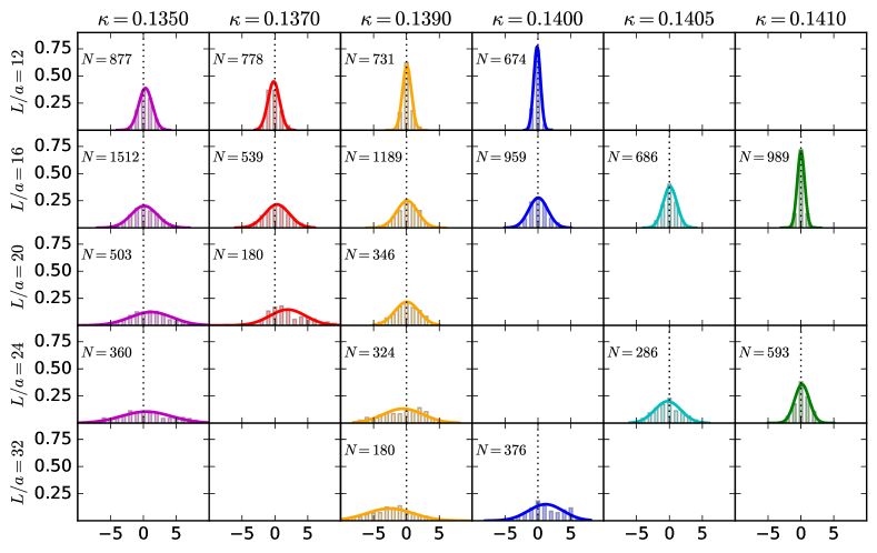
Figure 19: Topological charge distribution for the various ensembles.

Appendix B Results of the correlation function fits

Table 2 shows the relevant results obtained by fitting the reweighted and vacuum-subtracted correlation functions as described in Sec IV.

$L/a$	$\kappa$		Pseudoscalar			Vector			Scalar		$m_{\pi}^{\mathrm{fake}}$
			fit1	fit2	fit3	fit1	fit2	fit3	fit1	fit2
12	0.1350	gr	0.6503(24)	0.6468(18)	0.6497(23)	0.1944(90)	0.1800(68)	0.1884(82)	0.2248(70)	0.2189(68)	0.6457(13)
		ex	0.859(20)	0.787(29)	0.859(16)	0.6929(54)	0.6856(43)	0.6936(58)	0.739(10)	0.7632(88)
	0.1370	gr	0.5250(23)	0.5202(28)	0.5239(23)	0.1500(66)	0.1663(71)	0.1367(53)	0.1987(76)	0.1957(81)	0.5207(21)
		ex	0.794(12)	0.737(15)	0.7796(99)	0.5998(60)	0.6041(52)	0.5842(55)	0.6215(62)	0.6236(57)
	0.1390	gr	0.4246(28)	0.4238(30)	0.4262(27)	0.1237(41)	0.1110(42)	0.1115(33)	0.2117(84)	0.2113(89)	0.4229(36)
		ex	0.6845(87)	0.667(11)	0.7019(71)	0.5447(76)	0.470(10)	0.5091(61)	0.4613(37)	0.4809(39)
	0.1400	gr	0.4028(35)	0.4026(39)	0.4097(34)	0.1081(39)	0.1209(48)	0.1101(31)	0.272(21)	0.283(23)	0.4008(45)
		ex	0.6912(91)	0.683(14)	0.7198(87)	0.503(12)	0.530(11)	0.4916(86)	0.4307(50)	0.4432(58)
16	0.1350	gr	0.6371(25)	0.6367(31)	0.64301(92)	0.540(47)	0.370(43)	0.507(39)	0.352(14)	0.350(14)	0.64189(36)
		ex	0.901(31)	0.859(34)	0.832(16)	0.6765(70)	0.6734(39)	0.6809(19)	0.7858(88)	0.7848(78)
	0.1370	gr	0.5046(21)	0.5023(23)	0.5036(17)	0.356(41)	0.358(29)	0.396(31)	0.340(17)	0.374(22)	0.50102(84)
		ex	0.763(26)	0.786(35)	0.794(18)	0.5568(66)	0.5561(48)	0.5590(24)	0.6655(74)	0.6557(81)
	0.1390	gr	0.3506(21)	0.3517(21)	0.3506(20)	0.278(12)	0.309(11)	0.2782(96)	0.314(12)	0.320(13)	0.34695(93)
		ex	0.619(20)	0.618(31)	0.621(18)	0.4611(60)	0.4796(96)	0.4551(46)	0.4879(65)	0.4890(55)
	0.1400	gr	0.2782(34)	0.2798(35)	0.2777(33)	0.2118(76)	0.2134(69)	0.2203(60)	0.305(11)	0.318(13)	0.2623(17)
		ex	0.510(18)	0.514(25)	0.516(16)	0.4186(66)	0.4122(56)	0.4199(53)	0.4014(88)	0.3972(84)
	0.1405	gr	0.2419(36)	0.2418(46)	0.2398(36)	0.1768(74)	0.1819(70)	0.1872(58)	0.2856(56)	0.2977(77)	0.2239(38)
		ex	0.554(18)	0.563(32)	0.554(15)	0.3985(90)	0.4000(79)	0.4100(62)	0.3638(93)	0.368(10)
	0.1410	gr	0.1856(76)	0.173(10)	0.1760(65)	0.1595(78)	0.1520(61)	0.1554(66)	0.2639(78)	0.2651(87)	0.162(12)
		ex	0.468(18)	0.427(25)	0.462(14)	0.422(11)	0.4194(99)	0.4108(89)	0.310(10)	0.313(11)
20	0.1350	gr	0.6375(50)	0.6451(46)	0.6419(39)	0.6705(38)	0.6735(18)	0.6746(21)	0.484(37)	0.500(40)	0.64106(34)
		ex	0.815(36)	0.802(43)	0.805(76)	0.86(11)	0.936(40)	0.854(32)	0.8011(58)	0.7992(89)
	0.1370	gr	0.4978(42)	0.4990(42)	0.5006(35)	0.5442(17)	0.5400(25)	0.5430(18)	0.309(51)	0.356(68)	0.49905(77)
		ex	0.783(32)	0.777(21)	0.766(24)	0.737(19)	0.722(24)	0.711(19)	0.671(11)	0.6741(64)
	0.1390	gr	0.3344(13)	0.3325(15)	0.3353(14)	0.4004(10)	0.3982(14)	0.3993(10)	0.452(30)	0.466(17)	0.33608(80)
		ex	0.6757(92)	0.6686(70)	0.6683(90)	0.6387(73)	0.6030(92)	0.6193(70)	0.535(28)	0.596(49)
24	0.1350	gr	0.6484(25)	0.6488(15)	0.6480(22)	0.6777(15)	0.6759(11)	0.6757(12)	0.564(92)	0.71(13)	0.64141(26)
		ex	0.862(25)	0.852(36)	0.866(24)	0.861(29)	0.933(25)	0.873(24)	0.798(20)	0.834(28)
	0.1390	gr	0.3437(26)	0.3445(34)	0.3428(25)	0.39849(67)	0.39851(81)	0.39934(58)	0.443(24)	0.477(15)	0.33522(45)
		ex	0.601(18)	0.596(24)	0.602(18)	0.6159(68)	0.604(11)	0.6234(68)	0.530(23)	0.583(36)
	0.1405	gr	0.1930(30)	0.1942(33)	0.1957(29)	0.2791(15)	0.2804(16)	0.2815(14)	0.3649(51)	0.3553(51)	0.1691(14)
		ex	0.525(10)	0.513(12)	0.515(11)	0.5108(78)	0.5078(86)	0.5172(73)	0.623(42)	0.571(40)
	0.1410	gr	-	0.120(21)	0.117(12)	0.2466(28)	0.2423(28)	0.2451(27)	0.302(11)	0.264(18)	0.0673(57)
		ex	-	0.501(70)	0.468(58)	0.503(11)	0.491(13)	0.498(11)	0.598(42)	0.559(52)
32	0.1390	gr	0.3363(38)	0.3383(34)	0.3387(31)	0.40116(57)	0.4004(17)	0.40054(42)	0.475(11)	0.4933(93)	0.33484(42)
		ex	0.562(24)	0.556(34)	0.592(21)	0.585(23)	0.655(69)	0.616(16)	0.640(32)	0.691(49)
	0.1400	gr	0.2380(22)	0.2372(22)	0.2379(17)	0.31966(59)	0.32121(45)	0.31876(50)	0.4019(71)	0.3963(63)	0.23229(39)
		ex	0.541(18)	0.549(19)	0.553(12)	0.528(13)	0.640(20)	0.5240(98)	0.571(34)	0.564(26)

Table 2: Fit results from correlation function fits for the pseudoscalar, vector and scalar channels as well as the fake pion mass. Only statistical uncertainties are quoted.

Appendix C Determination of $t_{0}$

Table 3 shows values obtained for $t_{0}$ on each ensemble. We use two different action densities to compare systematic effects of setting the scale, i.e. the Wilson plaquette action ($t^{\mathrm{Wilson}}_{0}$) and the Yang-Mills action ($t^{\mathrm{YM}}_{0}$). As mentioned before, we quote these values only as reference for other lattice simulations. The quoted uncertainties originate from the numerical integration scheme and are statistical only. As an example we show the dependence of $t^{\mathrm{YM}}_{0}$ on the fake pion mass in Fig. 20. We note that $t_{0}^{\mathrm{YM}}$ displays large finite size effects for the smallest ensembles.

$L/a$	$\kappa$	$t^{\mathrm{Wilson}}_{0}/a^{2}$	$t^{\mathrm{YM}}_{0}/a^{2}$	$a^{\mathrm{Wilson}}$	$a^{\mathrm{YM}}$
12	0.1350	7.40(8)	7.10(5)	0.058(1)	0.060(1)
12	0.1370	8.25(8)	7.95(5)	0.055(1)	0.056(1)
12	0.1390	10.75(8)	10.40(15)	0.049(1)	0.049(1)
12	0.1400	12.55(8)	12.25(15)	0.045(1)	0.045(1)
16	0.1350	6.15(5)	5.95(5)	0.064(1)	0.065(1)
16	0.1370	6.60(5)	6.40(5)	0.062(1)	0.063(1)
16	0.1390	7.40(5)	7.20(5)	0.058(1)	0.059(1)
16	0.1400	8.10(5)	7.90(5)	0.056(1)	0.057(1)
16	0.1405	8.80(5)	8.55(5)	0.054(1)	0.054(1)
16	0.1410	10.10(5)	9.80(5)	0.050(1)	0.051(1)
20	0.1350	6.10(5)	5.85(5)	0.064(1)	0.066(1)
20	0.1370	6.50(5)	6.30(5)	0.062(1)	0.063(1)
20	0.1390	7.15(5)	6.95(5)	0.059(1)	0.060(1)
24	0.1350	6.05(5)	5.85(5)	0.065(1)	0.066(1)
24	0.1390	7.15(5)	6.95(5)	0.059(1)	0.060(1)
24	0.1405	8.05(5)	7.85(5)	0.056(1)	0.057(1)
24	0.1410	8.60(5)	8.35(5)	0.054(1)	0.055(1)
32	0.1390	7.10(5)	6.90(5)	0.060(1)	0.061(1)
32	0.1400	7.75(5)	7.50(5)	0.057(1)	0.058(1)

Table 3: Results for the $t_{0}$ using the Wilson flow Lüscher (2010). The quoted uncertainties are statistical only and discrete by construction, as the Wilson flow is numerically integrated and saved every step of length 0.05. We quote two estimates using the Wilson plaquette action ($t^{\mathrm{Wilson}}_{0}$) and the Yang-Mills action ($t^{\mathrm{YM}}_{0}$). The difference can be seen as an estimate for systematic uncertainties of the overall procedure.

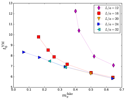
Figure 20: Results for the $t_{0}^{\mathrm{YM}}$ using the Wilson flow Lüscher (2010) as a function of fake pion mass. The equivalent plot for $t_{0}^{\mathrm{Wilson}}$ displays the same qualitative features.

References

- ’t Hooft (1974) G. ’t Hooft, Nucl. Phys. B 72, 461 (1974).
- Corrigan and Ramond (1979) E. Corrigan and P. Ramond, Phys. Lett. B 87, 73 (1979).
- Armoni et al. (2003a) A. Armoni, M. Shifman, and G. Veneziano, Nucl. Phys. B 667, 170 (2003a), arXiv:hep-th/0302163 .
- Armoni et al. (2003b) A. Armoni, M. Shifman, and G. Veneziano, Phys. Rev. Lett. 91, 191601 (2003b), arXiv:hep-th/0307097 .
- Sannino (2005) F. Sannino, Phys. Rev. D 72, 125006 (2005), arXiv:hep-th/0507251 .
- Sannino and Shifman (2004) F. Sannino and M. Shifman, Phys. Rev. D 69, 125004 (2004), arXiv:hep-th/0309252 .
- Armoni and Imeroni (2005) A. Armoni and E. Imeroni, Phys. Lett. B 631, 192 (2005), arXiv:hep-th/0508107 .
- Feo et al. (2004) A. Feo, P. Merlatti, and F. Sannino, Phys. Rev. D 70, 096004 (2004), arXiv:hep-th/0408214 .
- Creutz (2007) M. Creutz, Annals Phys. 322, 1518 (2007), arXiv:hep-th/0609187 .
- DeGrand et al. (2006) T. DeGrand, R. Hoffmann, S. Schaefer, and Z. Liu, Phys. Rev. D 74, 054501 (2006), arXiv:hep-th/0605147 .
- Leutwyler and Smilga (1992) H. Leutwyler and A. V. Smilga, Phys. Rev. D 46, 5607 (1992).
- Shuryak and Verbaarschot (1993) E. V. Shuryak and J. J. M. Verbaarschot, Nucl. Phys. A 560, 306 (1993), arXiv:hep-th/9212088 .
- Armoni et al. (2004) A. Armoni, M. Shifman, and G. Veneziano, Phys. Lett. B 579, 384 (2004), arXiv:hep-th/0309013 .
- Farchioni et al. (2007) F. Farchioni, I. Montvay, G. Munster, E. E. Scholz, T. Sudmann, and J. Wuilloud, Eur. Phys. J. C 52, 305 (2007), arXiv:0706.1131 [hep-lat] .
- Francis et al. (2018) A. Francis, R. J. Hudspith, R. Lewis, and S. Tulin, JHEP 12, 118 (2018), arXiv:1809.09117 [hep-ph] .
- Hambye and Tytgat (2010) T. Hambye and M. H. G. Tytgat, Phys. Lett. B 683, 39 (2010), arXiv:0907.1007 [hep-ph] .
- Athenodorou et al. (2021) A. Athenodorou, Bennett, G. Bergner, and B. Lucini, (2021), arXiv:2103.10485 [hep-lat] .
- Edwards et al. (1998a) R. G. Edwards, U. M. Heller, R. Narayanan, and J. Singleton, Robert L., Nucl. Phys. B 518, 319 (1998a), arXiv:hep-lat/9711029 .
- Edwards et al. (1998b) R. G. Edwards, U. M. Heller, and R. Narayanan, Nucl. Phys. B 535, 403 (1998b), arXiv:hep-lat/9802016 .
- Akemann et al. (2011) G. Akemann, P. Damgaard, K. Splittorff, and J. Verbaarschot, Phys. Rev. D 83, 085014 (2011), arXiv:1012.0752 [hep-lat] .
- Mohler and Schaefer (2020) D. Mohler and S. Schaefer, Phys. Rev. D 102, 074506 (2020), arXiv:2003.13359 [hep-lat] .
- Bergner and Wuilloud (2012) G. Bergner and J. Wuilloud, Comput. Phys. Commun. 183, 299 (2012), arXiv:1104.1363 [hep-lat] .
- Lucini et al. (2010) B. Lucini, G. Moraitis, A. Patella, and A. Rago, Phys. Rev. D 82, 114510 (2010), arXiv:1008.5180 [hep-lat] .
- Armoni et al. (2008) A. Armoni, B. Lucini, A. Patella, and C. Pica, Phys. Rev. D 78, 045019 (2008), arXiv:0804.4501 [hep-th] .
- Schaich (2023) D. Schaich, Eur. Phys. J. ST 232, 305 (2023), arXiv:2208.03580 [hep-lat] .
- Ziegler et al. (2022) F. P. G. Ziegler, M. Della Morte, B. Jäger, F. Sannino, and J. T. Tsang, PoS LATTICE2021, 225 (2022), arXiv:2111.12695 [hep-lat] .
- Della Morte et al. (2022) M. Della Morte, B. Jäger, S. Martins, F. Sannino, J. T. Tsang, and F. P. G. Ziegler, in 39th International Symposium on Lattice Field Theory (2022) arXiv:2212.06709 [hep-lat] .
- Iwasaki (1983) Y. Iwasaki, (1983), arXiv:1111.7054 [hep-lat] .
- Sheikholeslami and Wohlert (1985) B. Sheikholeslami and R. Wohlert, Nucl. Phys. B 259, 572 (1985).
- Lüscher (2010) M. Lüscher, JHEP 08, 071 (2010), [Erratum: JHEP 03, 092 (2014)], arXiv:1006.4518 [hep-lat] .
- Bruno and Sommer (2014) M. Bruno and R. Sommer (ALPHA), PoS LATTICE2013, 321 (2014), arXiv:1311.5585 [hep-lat] .
- (32) Lüscher, M. and Schäfer, S., “OpenQCD 1.6,” https://luscher.web.cern.ch/luscher/openQCD/.
- Clark and Kennedy (2007) M. A. Clark and A. D. Kennedy, Phys. Rev. Lett. 98, 051601 (2007), arXiv:hep-lat/0608015 .
- I.P. Omelyan and I.M. Mryglod and R. Folk (2003) I.P. Omelyan and I.M. Mryglod and R. Folk, Computer Physics Communications 151, 272 (2003).
- Luscher (2007a) M. Luscher, JHEP 12, 011 (2007a), arXiv:0710.5417 [hep-lat] .
- Luscher (2007b) M. Luscher, JHEP 07, 081 (2007b), arXiv:0706.2298 [hep-lat] .
- Itoh et al. (1987) S. Itoh, Y. Iwasaki, and T. Yoshie, Phys. Rev. D 36, 527 (1987).
- Morningstar et al. (2011) C. Morningstar, J. Bulava, J. Foley, K. J. Juge, D. Lenkner, M. Peardon, and C. H. Wong, Phys. Rev. D 83, 114505 (2011), arXiv:1104.3870 [hep-lat] .
- Peardon et al. (2009) M. Peardon, J. Bulava, J. Foley, C. Morningstar, J. Dudek, R. G. Edwards, B. Joo, H.-W. Lin, D. G. Richards, and K. J. Juge (Hadron Spectrum), Phys. Rev. D 80, 054506 (2009), arXiv:0905.2160 [hep-lat] .
- Brett et al. (2020) R. Brett, J. Bulava, D. Darvish, J. Fallica, A. Hanlon, B. Hörz, and C. Morningstar, AIP Conf. Proc. 2249, 030032 (2020), arXiv:1909.07306 [hep-lat] .
- Sommer et al. (2004) R. Sommer, S. Aoki, M. Della Morte, R. Hoffmann, T. Kaneko, F. Knechtli, J. Rolf, I. Wetzorke, and U. Wolff (ALPHA, CP-PACS, JLQCD), Nucl. Phys. B Proc. Suppl. 129, 405 (2004), arXiv:hep-lat/0309171 .
- Michael (1987) C. Michael, J. Phys. G 13, 1001 (1987).
- Michael and Perantonis (1992) C. Michael and S. J. Perantonis, J. Phys. G 18, 1725 (1992).
- Della Morte and Juttner (2010) M. Della Morte and A. Juttner, JHEP 11, 154 (2010), arXiv:1009.3783 [hep-lat] .
- Gell-Mann et al. (1968) M. Gell-Mann, R. J. Oakes, and B. Renner, Phys. Rev. 175, 2195 (1968).
- Farchioni et al. (2008) F. Farchioni, G. Munster, T. Sudmann, J. Wuilloud, I. Montvay, and E. E. Scholz, PoS LATTICE2008, 128 (2008), arXiv:0810.0161 [hep-lat] .