Homotopy solution to non-linear evolution for heavy nuclei

Abstract

In the paper we suggest the homotopy method for solving of the non linear evolution equation. This method consists of two steps. First is the analytical solution for the linearized version of the non-linear evolution deep in the saturation region. Second, the perturbative procedure is suggested to take into account the remaining parts of the non-linear corrections. It turns out that these corrections are rather small and can be estimated in the regular iterative procedure.

I Introduction

The Colour Glass Condensate approachGLR ; MUQI ; MUCD ; MV ; KLBOOK ; BK ; JIMWLK (CGC) has reached a mature stage and has become the common language to discuss high energy scattering where the dense system of partons (quarks and gluons) is produced. The most theoretical progress has been reached in the description of dilute-dense parton system scatteringREV . The deep inelastic scattering (DIS) of electron with hadrons is well known example of such process. For these processes we know their main qualitative features as well as the non-linear evolution equationBK ; JIMWLK , that describes them. For DIS with protons it has been shown that at high energies the density of partons reaches the saturation and dipole-hadron amplitude tends to approach unityGLR . The analytical form of the scattering amplitude at high energies has been foundLT . At high energies the scattering amplitude shows the scaling behaviour LT ; BALE ; SGBK ; IIM , which leads to the amplitude being a function of one variable $x^{2}_{10}Q^{2}_{s}(Y,b)$. In two regions we have the analytical solution to the non-linear Balitsky-KovchegovBK (BK) equation: (i) for $x^{2}_{10}Q^{2}_{s}(Y,b)\,\,\gg\,\,1$LT and (ii) for $x^{2}_{10}Q^{2}_{s}(Y,b)\,\,\sim\,\,1$MUT .

In other words, the non-linear evolution BK equation for the scattering amplitude $N_{ik}=N\left(Y,\boldsymbol{x}_{ik},\boldsymbol{b}\right)$ has the following general form:

$$\frac{\partial N_{01}}{\partial Y}\,=\,\bar{\alpha}_{S}\int\frac{d^{2}\,x_{02}}{2\pi}\frac{x^{2}_{01}}{x^{2}_{02}\,x^{2}_{12}}\Big{\{}N_{02}+N_{12}-N_{02}N_{12}-N_{01}\Big{\}}$$ (1)

and it has the analytical solutions in these two regions. Indeed, for $x^{2}_{10}Q^{2}_{s}(Y)\,\,\gg\,\,1$ the scattering amplitude approaches unity and has the formLT :

$$N_{01}\left(z\right)\,\,\,=\,\,1\,\,\,-\,\,\,\mbox{Const}\,\exp\Big{(}-\frac{z^{2}}{2\,\kappa}\Big{)}$$ (2)

where $z$ and $\kappa$ are determined by the following equations:

$$\kappa\,\,\equiv\,\,\frac{\chi\left(\gamma_{cr}\right)}{1-\gamma_{cr}}\,\,=\,\,-\frac{d\chi\left(\gamma_{cr}\right)}{d\gamma_{cr}}~{}~{}~{}\,\,\,\mbox{and}\,\,\,~{}~{}~{}\chi\left(\gamma\right)\,=\,\,2\,\psi\left(1\right)\,-\,\psi\left(\gamma\right)\,-\,\psi\left(1-\gamma\right)$$ (3)

and for new variable $z$ we have

$$z\,\,=\,\,\ln\left(x^{2}_{01}\,Q^{2}_{s}\left(Y,b\right)\right)\,\,\,=\,\,\,\,\bar{\alpha}_{S}\,\kappa\,\left(Y\,-\,Y_{A}\right)\,\,+\,\,\xi\,\,\,=\,\,\xi_{s}\,\,+\,\,\xi$$ (4)

where $\xi\,\,=\,\,\ln\left(x^{2}_{10}\,Q^{2}_{s}\left(Y=Y_{A},b\right)\right)$ and $Q^{2}_{s}(Y,b)$ is equal to

$$Q^{2}_{s}\left(Y,b\right)\,\,=\,\,Q^{2}_{s}\left(Y=Y_{A},b\right)\,e^{\bar{\alpha}_{S}\,\kappa\left(Y-Y_{A}\right)}\$$ (5)

In Eq. (4) and Eq. (5) $Y_{A}$ denotes $Y_{A}=\ln A^{1/3}$, where $A$ is the number of nucleons in a nucleus.

In the vicinity of the saturation scale $x^{2}_{10}\,Q^{2}_{s}\left(Y,b\right)\,\sim\,1$ the scattering amplitude has the formMUT :

$$N_{01}\left(z\right)\,\,\,=\,\,\,\mbox{Const}\left(x^{2}_{10}\,Q^{2}_{s}\left(Y,b\right)\right)^{\bar{\gamma}}$$ (6)

with $\bar{\gamma}=1-\gamma_{cr}$.

From Eq. (6) one can see that at $x_{01}\,Q_{s}=1(z=0)$ we have the following boundary conditions for the saturation region:

$$N_{01}\left(z=0\right)\,\,=\,\,N_{0};~{}~{}~{}~{}~{}~{}~{}~{}\frac{dN_{01}\left(z\right)}{d\,z}\Bigg{|}_{z=0}\,\,=\,\,\bar{\gamma}\,N_{0}.$$ (7)

Finally, for $x^{2}_{10}\,Q^{2}_{s}\left(Y,b\right)\,\ll\,1$ the scattering amplitude satisfies the linear BFKL equation and is a function of two variables: $Y$ and $\xi$.

We have defined the saturation region as $x^{2}_{10}\,Q^{2}_{s}\left(Y,b\right)\,>\,1$. However, in Refs.GOST ; BEST it has been noted that actually for very large $x_{10}$ the non-linear corrections are not important and we have to solve linear BFKL equation. This feature can be seen directly from the eigenfunction of this equation. Indeed, the eigenfunction (the scattering amplitude of two dipoles with sizes $r\equiv x_{10}$ and $R$) has the following form LIP

$$\phi_{\gamma}\left(\boldsymbol{r},\boldsymbol{R},\boldsymbol{b}\right)\,\,\,=\,\,\,\left(\frac{r^{2}\,R^{2}}{\left(\boldsymbol{b}+\frac{1}{2}(\boldsymbol{r}-\boldsymbol{R})\right)^{2}\,\left(\boldsymbol{b}-\frac{1}{2}(\boldsymbol{r}-\boldsymbol{R})\right)^{2}}\right)^{\gamma}~{}~{}~{}~{}\mbox{with}\,\,0\,<\,Re\gamma\,<\,1$$ (8)

One can see that for $r=x_{10}\,>\,min[R,b]$, $\phi_{\gamma}$ starts to be small and the non-linear term in the BK equation could be neglected. In this paper we consider the interaction with nucleus and the scattering amplitude of the dipole with a nucleus for the exchange of the BFKL Pomeron has the following form:

$$A_{dA}\left(\boldsymbol{r},\boldsymbol{R}_{N},\boldsymbol{b}\right)\,=\,\phi_{\gamma}\left(\boldsymbol{r},\boldsymbol{R}_{N},\boldsymbol{c}\right)\,\,S_{A}\left(\boldsymbol{b}-\boldsymbol{c}\right)d^{2}c$$ (9)

where $R_{N}$ is the size of a nucleon, $\boldsymbol{c}$ is the impact parameter for dipole-nucleon amplitude and $\boldsymbol{b}-\boldsymbol{c}$ is the position of the nucleon with respect to the center of the nucleus. $S_{A}\left(\boldsymbol{b}-\boldsymbol{c}\right)$ is the number of nucleons in a nucleus. Since $c\,\ll\,b$ we can integrate over $\boldsymbol{c}$ replacing $\boldsymbol{b}-\boldsymbol{c}$ by $\boldsymbol{b}$ and obtain the expression:

$$A_{dA}\left(\boldsymbol{r},\boldsymbol{R}_{N},\boldsymbol{b}\right) = \int\phi_{\gamma}\left(\boldsymbol{r},\boldsymbol{R}_{N},\boldsymbol{c}\right)\,\,S_{A}\left(\boldsymbol{b}-\boldsymbol{c}\right)d^{2}c=\int d^{2}c\,\phi_{\gamma}\left(\boldsymbol{r},\boldsymbol{R}_{N},\boldsymbol{c}\right)\,\,S_{A}\left(\boldsymbol{b}\right)$$ (10)

$$= \left(\frac{r^{2}}{R^{2}_{N}}\right)^{\gamma}\!\!R^{2}_{N}S_{A}\left(\boldsymbol{b}\right)=\left(r^{2}\,Q^{2}_{s}\left(Y=Y_{A},b\right)\right)^{\gamma}\,$$

Therefore, in this case we can absorb all dependence on the impact parameter in the $b$ dependence of the saturation scale. In Eq. (10) we implicitly assume that $r\leq R_{N}$. The typical process, that we bear in mind, is the deep inelastic scattering(DIS) with a nucleus at $Q^{2}\,\geq\,1GeV^{2}$ and at small values of $x$.

For getting more quantitative information, which is needed for comparison with the experimental data, the BK equation has to be solved numerically. However, the CGC approach suffers the principle difficulty: the power-like behaviour of the scattering amplitude at large impact parameters $b$ KW1 ; KW2 ; KW3 ; FIIM , which leads the violation of the Froissart theorem FROI . The widely accepted phenomenological way to heal this problem is to introduce the non-perturbative dependence of $Q^{2}_{s}\left(Y=0,b\right)\propto\exp\left(-\mu\,b\right)$ (see Refs.IIMU ; BKL ; RESH ; CLP and references therein). One can see that a numerical solution of the BK equation does not allow us to introduce these corrections since the BK equation does not have an explicit dependence on $Q_{s}$. The standard way of dealing with the non-perturbative corrections is to change the BFKL kernel introducing a soft scale. In doing this we violate the conformal symmetry of the kernel, which is the basis of our understanding of many features of the solution. We consider the non-perturbative corrections to the saturation scale, which the new and the only dimensional scale in our problem, as more attractive way of introducing the soft scale. Bearing this in mind we need to have the analytical solution in which we can see explicitly the dependence of the scattering amplitude on $Q_{s}(Y,b)$.

In this paper we have two goals. First we suggest a procedure to find the solution to the BK equation as a sequence of iterations, based on homotopy approach HE1 ; HE2 . This approach gives us a tool to introduce the saturation momentum in our calculation, starting from the first iteration, and allow us the insert the non-perturbative changes in $b$ dependence of $Q_{s}(b)$.

The homotopy method we can use in the case when you equation has a general form:

$$\mathscr{L}[u]+\mathscr{N_{L}}[u]=0$$ (11)

where the linear part $\mathscr{L}[u]$ is a differential or integral-differential operator, but non-linear part $\mathscr{N_{L}}[u]$ has an arbitrary form. For solution we introduce the following equation for the homotopy function ${\cal H}\left(p,u\right)$:

$${\cal H}\left(p,u\right)\,\,=\,\,\mathscr{L}[u_{p}]\,+\,p\,\mathscr{N_{L}}[u_{p}]\,\,=\,\,0$$ (12)

Solving Eq. (12) we reconstruct the function

$$u_{p}\left(Y,\boldsymbol{x}_{10},\boldsymbol{b}\right)\,\,=\,\,u_{0}\left(Y,\boldsymbol{x}_{10},\boldsymbol{b}\right)\,\,+\,\,p\,u_{1}\left(Y,\boldsymbol{x}_{10},\boldsymbol{b}\right)\,+\,p^{2}\,u_{3}\left(Y,\boldsymbol{x}_{10},\boldsymbol{b}\right)\,\,+\,\,\dots$$ (13)

with $\mathscr{L}[u_{0}]=0$. Eq. (13) gives the solution to the non-linear equation at $p$=1. The hope is that several terms in series of Eq. (13) will give a good approximation to the solution of the non-linear equation. This method has been applied to the solution of the BK equationSPS , but we suggest a quite different procedure that allow us to see the geometric scaling behaviour as well as the dependence on the saturation scale in explicit form on each stage of the solution.

The second goal of this paper is to find the efficient procedure to solve the BK equation for interaction with nuclei. In this case, as the initial conditions at $Y=Y_{A}$ for DIS with nuclei we have McLerran-Venugopalan formulaMV for the imaginary part of the dipole-nucleus amplitude, which takes the following form (see Fig. 1)

$$N\left(x^{2}_{10},Y=Y_{A},b\right)\,\,\,=\,\,1\,\,\,-\,\,\,\exp\Big{(}-r^{2}\,Q^{2}_{s}\left(Y=Y_{A},b\right)/4\Big{)}\,\,=\,\,1\,\,\,-\,\,\exp\left(-\frac{1}{4}\,e^{\xi}\right)$$ (14)

where $r=x_{10}$ and we will use this notation for the size of the dipole below.

One can see from Fig. 1, that for large $Y_{A}\,=\,\frac{1}{3}\ln A$, these initial conditions, which violate the geometric scaling behaviour, give the scattering amplitude in the saturation region. Comparing Eq. (14) and Eq. (2) we see that the geometric scaling behaviour cannot be correct in the entire saturation region. This problem is not new and we have discussed it in our previous papers LTHI ; KLT ; CLM . Having a new iteration procedure we hope to suggest a practical way to take into account the initial conditions of Eq. (14).

Eq. (14) in the region, where we can trust perturbative QCD, has the form: $\frac{1}{4}e^{\xi_{0}^{A}}$. Hence the equation for $\xi_{0}^{A}$(see Fig. 1) takes the following form:

$$\frac{1}{4}e^{\xi_{0}^{A}}\,=\,\,\mbox{Const}\left(x^{2}_{10}\,Q^{2}_{s}\left(Y,b\right)\right)^{\bar{\gamma}}$$ (15)

It should be noted that Eq. (7) for any value of $z$ in the vicinity of the saturation scale: $x^{2}_{10}\,Q^{2}_{s}\left(Y,b\right)\,\sim\,1$.

In the next section we introduce the non-linear Balitsky-Kovchegov equation in the momentum space and discuss the homotopy approach for solving this equation. The suggested approach consists of two steps. First, we introduce the linearized vesion of the non-linear equation deep in the saturation region.Using the solution of this linear equation we develop the homotopy approach that gives us a regular procedure how to take into account the non-linear correction which could be sizable in the saturation region. In section 3 we discuss in detail the first two iterations of the homotopy approach. In particular, we demonstrate that the first iteration gives a rather small contribution. This, in our opinion, indicates that the homotopy approach gives the regular way to account the non-linear corrections, which are non-perturbative in their origin, in the perturbative way after subtracting the contributions of them deep in the saturation region. In conclusions we summarize our results.

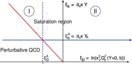
Figure 1: Saturation region of QCD. The critical line (z=0) is shown in red. The initial condition for scattering with the dilute system of partons (with proton) is given at $\xi_{s}=0$. For heavy nuclei the initial conditions are placed at $Y_{A}=(1/3)\ln\,A\gg\,1$, where $A$ is the number of nucleon in a nucleus. The line, where they are given, is shown in blue.

II Equation and solution in the momentum space

II.1 Rewriting BK equation in the convenient for the homotopy approach form

We re-write the Balitsky-Kovchegov equation of Eq. (1) in the momentum space introducing

$$N\left(r^{2},b,Y\right)\,\,=\,\,r^{2}\,\int\frac{d^{2}k_{\perp}}{2\pi}\,e^{i\boldsymbol{k}_{\perp}\cdot\boldsymbol{r}}\,\widetilde{N}\left(k_{\perp},b,Y\right)\,=\,r^{2}\int\limits^{\infty}_{0}k_{\perp}dk_{\perp}J_{0}\left(rk_{\perp}\right)\,\widetilde{N}\left(k_{\perp},b,Y\right)$$ (16)

In Eq. (16) we assume that the amplitude has radial symmetry and it takes the formGLR ; KOV

$$\frac{\partial\widetilde{N}\left(k_{\perp},b,Y\right)}{\partial Y}\,\,=\,\,\bar{\alpha}_{S}\Bigg{\{}\chi\left(-\,\frac{\partial}{\partial\tilde{\xi}}\right)\widetilde{N}\left(k_{\perp},b,Y\right)\,\,\,-\,\,\widetilde{N}^{2}\left(k_{\perp},b,Y\right)\Bigg{\}}$$ (17)

where

$$\tilde{\xi}\,\,=\,\,\,\,\ln\left(Q^{2}_{s}\left(Y=Y_{A},b\right)/k^{2}_{\perp}\right)~{}~{}~{}\mbox{and}~{}~{}~{}\tilde{z}\,\,=\,\,\bar{\alpha}_{S}\kappa\left(Y-Y_{A}\right)\,\,+\,\,\tilde{\xi}\,\,=\,\,\ln\left(Q^{2}_{s}\left(Y,b\right)/k^{2}_{\perp}\right)$$ (18)

The advantage of the non-linear equation in Eq. (17), that the non-linear term depends only on external variables and does not contain the integration over momenta. The BFKL kernelBFKL : $\chi\left(-\,\frac{\partial}{\partial\tilde{\xi}}\right)$, can be written as the series over positive powers of $\partial/\partial\tilde{\xi}$ except of the first term

$$\frac{1}{\gamma}\,\widetilde{N}\left(\gamma,b,Y\right)\,\,\,\to\,\,\,\int\limits^{k^{2}_{\perp}}\frac{dk^{\prime 2}_{\perp}}{k^{\prime 2}_{\perp}}\widetilde{N}\left(k^{\prime}_{\perp},b,Y\right)$$ (19)

where $\widetilde{N}\left(\gamma,b,Y\right)$ is the image of the scattering amplitude in $\gamma$-representation:

$$\widetilde{N}\left(k_{\perp},b,Y\right)=\int\limits^{\epsilon+i\infty}_{\epsilon-i\infty}\!\!\!\frac{d\gamma}{2\pi i}\left(k^{2}_{\perp}\right)^{\gamma}\widetilde{N}\left(\gamma,b,Y\right).$$ (20)

Differentiating Eq. (17) over $\tilde{\xi}$ one can see that it can be re-written as

$$\frac{\partial^{2}\widetilde{N}\left(k_{\perp},b,Y\right)}{\partial Y\,\partial\tilde{\xi}}\,\,\,=$$ (21)

$$\,\,\,\bar{\alpha}_{S}\Bigg{\{}\chi_{0}\left(-\frac{\partial}{\partial\tilde{\xi}}\right)\,\,\frac{\partial\widetilde{N}\left(k_{\perp},b,Y\right)}{\partial\,\tilde{\xi}}\,\,+\,\,\widetilde{N}\left(k_{\perp},b,Y\right)\,\,-\,\,2\frac{\partial\widetilde{N}\left(k_{\perp},b,Y\right)}{\partial\,\tilde{\xi}}\widetilde{N}\left(k_{\perp},b,Y\right)\Bigg{\}}$$

with $\chi_{0}(\gamma)\,=\,\chi(\gamma)\,\,-\dfrac{1}{\gamma}$ where $\chi\left(\gamma\right)$ is given by Eq. (3).

Introducing the variable $\tilde{z}$ instead of $\tilde{\xi}$ and the new functions $M$ and $\Phi$ as

$$\frac{\partial\widetilde{N}\left(k_{\perp},b,Y\right)}{\partial\,\tilde{z}}\,\,=\,\,\frac{1}{2}+M\left(\tilde{z},b,\delta\tilde{Y}\right)~{}~{}~{}~{}\mbox{or}~{}~{}~{}~{}\widetilde{N}\left(\tilde{z},b,\delta\tilde{Y}\right)\,\,=\,\,\frac{1}{2}\tilde{z}\,\,+\,\,\int\limits^{\tilde{z}}_{0}d\tilde{z}^{\prime}M\left(\tilde{z}^{\prime},b,Y\right)\,\,+\,\,\Phi\left(\delta\tilde{Y}\right)$$ (22)

we can re-write Eq. (21) in the form

$$\frac{\partial M\left(\tilde{z},b,\delta\tilde{Y}\right)}{\partial\delta\tilde{Y}}\,\,+\,\,\kappa\,\frac{\partial M\left(\tilde{z},b,\delta\tilde{Y}\right)}{\partial\tilde{z}}\,\,\,=\chi_{0}\left(\frac{\partial}{\partial\tilde{z}}\right)\ M\left(\tilde{z},b,\delta\tilde{Y}\right)\,\,-\,\,\,\tilde{z}\,M\left(\tilde{z},b,\delta\tilde{Y}\right)\,\ -2\,\Phi\left(\delta\tilde{Y}\right)\,M\left(\tilde{z},\delta\tilde{Y}\right)\,\,-\dfrac{\partial A}{\partial\tilde{z}}$$ (23)

with $\delta\tilde{Y}=\overline{\alpha}_{S}\left(Y-Y_{A}\right)$ and

$$A(\tilde{z},b,\delta\tilde{Y})=\left(\int_{0}^{\tilde{z}}M(z^{\prime},b,\delta\tilde{Y})dz^{\prime}\right)^{2}$$ (24)

In Eq. (22) we introduce a new function $M$, which approaches zero at large $\tilde{z}$, since $\frac{1}{2}$ is the correct asymptotic behaviour in the momentum representation. It corresponds to the amplitude in the coordinate representation, that is equal to unity deep in the saturation region.

Looking for $N(r,b,Y)$, that depend only on |r|, we can rewrite Eq. (16) as follows

$$\widetilde{N}(k_{\perp},b,\delta\tilde{Y})=\int\limits_{0}^{\infty}rdr\dfrac{J_{0}(rk_{\perp})}{r^{2}}N(r,b,\delta\tilde{Y})$$ (25)

On the other hands, differentiating Eq. (25) with respect to $k_{\perp}$ we have

$$\dfrac{\partial\widetilde{N}(k_{\perp},b,\delta\tilde{Y})}{\partial k_{\perp}}=-\int\limits_{0}^{\infty}drJ_{1}(rk_{\perp})N(r,b,\delta\tilde{Y})$$ (26)

From Eq. (22) and Eq. (26) we obtain for $M(\tilde{z},b,\delta\tilde{Y})$ the following formula:

$$M(\tilde{z},b,\delta\tilde{Y})\,\,=\,\,k_{\perp}\int\limits_{0}^{\infty}drJ_{1}(rk_{\perp})\Bigg{\{}\frac{N(r,b,\delta\tilde{Y})\,\,-\,\,1}{2}\Bigg{\}}$$ (27)

II.2 Homotopy approach

We rewrite the non-linear evolution equation in momentum representation (see Eq. (23)), choosing the linear and non-linear parts of the BK equation, in the following form:

$$\mathscr{L}[F]=\dfrac{\partial F}{\partial\tilde{Y}}+\kappa\dfrac{\partial F}{\partial\tilde{z}}-\chi_{0}\left(\dfrac{\partial}{\partial\tilde{z}}\right)F+\tilde{z}F+2\,\Phi\left(\delta\tilde{Y}\right)\,F\,,\quad\mathscr{N_{L}}[F]=\dfrac{\partial}{\partial\tilde{z}}\left(\int\limits_{0}^{\tilde{z}}Fdz^{\prime}\right)^{2}$$ (28)

The homotopy equation takes the following form:

$${\cal H}\left(p,M_{p}(\tilde{z},b,\delta\tilde{Y})\right)\,\,=\,\,\mathscr{L}[M_{p}]+p\mathscr{A}_{p}\,\,=\,\,0$$ (29)

We are looking for the solution of Eq. (28) in the form:

$$F\,\equiv\,\,M_{p}(\tilde{z},b,\delta\tilde{Y})=\sum_{n=0}^{\infty}M_{n}(\tilde{z},b,\delta\tilde{Y})\,p^{n}$$ (30)

Plugging Eq. (30) into the homotopy equation (see Eq. (29)) we obtain the following equation for functions $M_{n}$:

$$\mathscr{L}[M_{n}]+p\mathscr{A}_{n-1}\,\,=\,\,0$$ (31)

where $\mathscr{A}_{p}=\sum_{n=0}^{\infty}A_{n}(\tilde{z},b,\delta\tilde{Y})p^{n}$ being

$$A_{n}(\tilde{z},b,\delta\tilde{Y})=\sum_{j=0}^{n}\left(\int\limits_{0}^{\tilde{z}}M_{j}(z^{\prime},b,\delta\tilde{Y})\right)\left(\int\limits_{0}^{\tilde{z}}M_{n-j}(z^{\prime},b,\delta\tilde{Y})\right)$$ (32)

In the explicit form Eq. (31) takes the form:

$$\dfrac{\partial M_{n}}{\partial\tilde{Y}}+\kappa\dfrac{\partial M_{n}}{\partial\tilde{z}}=\chi_{0}\left(\dfrac{\partial}{\partial\tilde{z}}\right)M_{n}-\tilde{z}M_{n}-2\,\sum_{j=0}^{n}\Phi_{n-j}\left(\delta\tilde{Y}\right)\,M_{j}-\dfrac{\partial A_{n-1}}{\partial\tilde{z}}$$ (33)

where $\Phi\left(\delta\tilde{Y}\right)\,\,=\,\,\sum_{n}\,\Phi_{n}\left(\delta\tilde{Y}\right)\,p^{n}$. As we discuss below, we start from finding solution at $p=0$ which satisfies Eq. (7) at $z=\xi^{A}_{0}$ and Eq. (14) at $\delta\tilde{Y}=0$. It turns out that we need to introduce $\Phi_{0}\left(\delta\tilde{Y}\right)=\frac{1}{2}\zeta$. For such $\Phi_{0}$ Eq. (33) can be rewritten in the form:

$$\dfrac{\partial M_{n}}{\partial\tilde{Y}}+\kappa\dfrac{\partial M_{n}}{\partial\tilde{z}}=\chi_{0}\left(\dfrac{\partial}{\partial\tilde{z}}\right)M_{n}-\left(\tilde{z}\,+\,\zeta\right)M_{n}-2\,\sum_{j=0}^{n-1}\Phi_{n-j}\left(\delta\tilde{Y}\right)\,M_{j}-\dfrac{\partial A_{n-1}}{\partial\tilde{z}}$$ (34)

In the case of $n=0$ we do not have two last terms of Eq. (34).

III Solution in the saturation region

III.1 Zero iteration (p=0) solution

For $p=0$ we need to solve the linear equation for $M_{0}(\tilde{z},b,\delta\tilde{Y})$. The equation does not depend on $A(\tilde{z},b,\delta\tilde{Y})$ of Eq. (24) but the term $\tilde{z}M_{0}$ in Eq. (33) actually stems from the term $\tilde{N}^{2}$ in the BK equation.

From Eq. (34) we see that the equation for $M_{0}(\tilde{z},b,\delta\tilde{Y})$ takes the form:

$$\dfrac{\partial M_{0}}{\partial\,\delta\tilde{Y}}+\kappa\dfrac{\partial M_{0}}{\partial\tilde{z}}=\chi_{0}\left(\dfrac{\partial}{\partial\tilde{z}}\right)M_{0}-(\tilde{z}+\zeta)M_{0}$$ (35)

The particular solution to this equation depends only on $\tilde{z}$ and it can be found from the equation:

$$\kappa\frac{dM_{0}\left(\tilde{z},b\right)}{d\tilde{z}}\,\,\,=\,\,\,\chi_{0}\left(\dfrac{d}{d\tilde{z}}\right)M_{0}\left(\tilde{z},b\right)\,\,-\,\,\,(\tilde{z}\,+\,\zeta)\,M_{0}\left(\tilde{z},b\right)$$ (36)

We are looking for the solution, which has the following form in two kinematic regions, which are shown in Fig. 1

$$M_{0}\left(\tilde{z},\delta\tilde{Y}\right)\,\,=\,\,\left\{\begin{array}[]{l}\,\,M^{I}_{0}\left(\tilde{z}\right)\,\,\,\,\,\,\,\,\,\,\mbox{for}\,\,\,\,-\kappa\delta\tilde{Y}\,\,<\,\,\tilde{\xi}\,\,<\,\tilde{\xi}^{A}_{0};\\ \\ \,\,M^{II}_{0}\left(\tilde{z},\delta\tilde{Y}\right)\,\,\,\,\,\mbox{for}\,\,\,\tilde{\xi}\,>\,\tilde{\xi}^{A}_{0};\\ \end{array}\right.$$ (40)

where $M_{0}^{II}\left(\tilde{z},\delta\tilde{Y}\right)$ is the solution to the general equation (see Eq. (35)). Note, that we use the momentum representation instead of the coordinate one, which is shown in Fig. 1. Eq. (18) leads to $\xi^{A}=\ln\left(r^{2}Q^{2}_{A}(Y_{A},b)\right)\to\tilde{\xi}^{A}=\ln\left(Q^{2}_{A}(Y_{A},b)/k^{2}_{T}\right)$. The boundary and initial conditions for $M_{0}\left(\tilde{z},\delta\tilde{Y}\right)$ in the saturation region we take the same as for the full equation (see Eq. (23) and Fig. 1):

$$\mbox{region}\,I: M^{I}_{0}\left(\tilde{z}\,=\,\tilde{\xi}_{0}^{A},b\right)=\,\phi_{0}(b)-\frac{1}{2}=M_{0}~{}~{}~{}~{}~{}\phi_{0}(b)\,\ll\,\frac{1}{2};\,\,$$ (41a)

$$\mbox{region}\,II: M^{II}_{0}(\tilde{z},\delta\tilde{Y}=0;b)=-\dfrac{1}{2}\left(1-\exp(-\exp(-\tilde{\xi}))\right),M_{0}=-\dfrac{1}{2}\left(1-\exp(-\exp(-\tilde{\xi}^{A}_{0}))\right)~{}\mbox{for}~{}\tilde{\xi}>\tilde{\xi}^{A}_{0}\,\,$$ (41b)

Note, that this equation for $\tilde{\xi}\,>\,\tilde{\xi}^{A}_{0}$ we obtain directly from McLerran-Venugopalan formula of Eq. (14), using Eq. (27). $\phi_{0}\left(b\right)$ is the value of the scattering amplitude at $\tilde{z}=\tilde{\xi}^{A}_{0}$. As one can see from these equations, we put the boundary condition of Eq. (41a) for the $M^{I}_{0}$ while for $M^{II}_{0}$ we are using the initial condition of Eq. (14).

III.1.1 Geometric scaling solution $M^{I}_{0}\left(\tilde{z}\right)$

We solve Eq. (36) using the Mellin transform

$$M_{0}\left(\tilde{z},b\right)=\int\limits^{\epsilon+i\infty}_{\epsilon-i\infty}\frac{d\gamma}{2\pi i}e^{\gamma(\tilde{z}+\zeta)}m_{0}\left(\gamma,b\right)$$ (42)

where $m_{0}\left(\gamma,b\right)$ satisfies the equation:

$$\left(\kappa\gamma-\chi\left(\gamma\right)+1/\gamma\right)\,m_{0}\left(\gamma,b\right)=\frac{dm_{0}\left(\gamma,b\right)}{d\gamma}.$$ (43)

The solution for $m_{0}\left(\gamma,b\right)$ takes the following form

$$m_{0}\left(\gamma\right)\,\,=\,\,m(0)\exp\Bigg{(}\int\limits^{\gamma}_{0}d\gamma^{\prime}\Big{(}\kappa\gamma^{\prime}-\chi\left(\gamma^{\prime}\right)+1/\gamma^{\prime}\Big{)}\Bigg{)}$$ (44)

Taking into account the explicit form of the BFKL kernel given by Eq. (3) one can re-write Eq. (44) in the form of the product of two Mellin’s transforms

$$m_{0}\left(\gamma\right)\,\,=\,\,m(0)\exp\Bigg{(}\kappa\gamma^{2}/2-2\psi(1)\gamma\Bigg{)}\,\Bigg{(}\frac{\gamma\Gamma(\gamma)}{\Gamma(1-\gamma)}\Bigg{)}$$ (45)

In Eq. (44) and Eq. (45)

$$m(0)=\frac{\phi_{0}(b)-(1/2)}{C\left(\zeta\right)}~{}~{}~{}~{}\mbox{where}~{}~{}~{}C\left(\zeta\right)=\int\limits^{\epsilon+i\infty}_{\epsilon-i\infty}\dfrac{d\gamma}{2\pi i}e^{(\zeta+2\psi(1))\gamma}e^{\frac{1}{2}\kappa\gamma^{2}}\frac{\Gamma\left(1+\gamma\right)}{\Gamma\left(1-\gamma\right)}.$$

From Eq. (45) we obtain

$$M_{0}^{I}(\tilde{z})\,=\,\int_{\epsilon-i\infty}^{\epsilon+i\infty}\dfrac{d\gamma}{2\pi i}e^{\gamma(\delta\tilde{Y}+\zeta)}\,m(0)\,\left(\dfrac{k_{\perp}}{Q_{s}(Y_{A},b)}\right)^{-2\gamma}\dfrac{\Gamma(1+\gamma)}{\Gamma(1-\gamma)}e^{\kappa\gamma^{2}/2}e^{-2\psi(1)\gamma}$$ (46)

Formula 6.561.14 of Ref.RY leads to the following expression in the coordinate representation:

$$\int_{0}^{\infty}M_{0}^{I}(\tilde{z})J_{1}(k_{\perp}r)dk_{\perp}\,=\,\dfrac{m(0)}{r}\,\int_{\epsilon-i\infty}^{\epsilon+i\infty}\dfrac{d\gamma}{2\pi i}\left(\dfrac{r^{2}Q_{s}^{2}(Y_{A},b)\,e^{\kappa\delta\tilde{Y}+\zeta-2\psi(1)}}{4}\right)^{\gamma}\,e^{\kappa\gamma^{2}/2}$$ (47)

Taking into account Eq. (27) and using

$$\int_{0}^{\infty}k_{\perp}\,dk_{\perp}\,J_{1}(k_{\perp}\,r)J_{1}(k_{\perp}r^{\prime})\,=\,\dfrac{1}{r}\delta(r-r^{\prime})$$ (48)

we reduce Eq. (47) to

$$N^{I}_{0}(z)\,=\,1\,+\,2\,m(0)\,\int_{\epsilon-i\infty}^{\epsilon+i\infty}\dfrac{d\gamma}{2\pi i}\left(\dfrac{r^{2}Q_{s}^{2}(Y_{A},b)\,e^{\kappa\delta\tilde{Y}+\zeta-2\psi(1)}}{4}\right)^{\gamma}\,e^{\kappa\gamma^{2}/2}$$ (49)

Introducing $z=\kappa\delta\tilde{Y}+\ln(r^{2}Q_{s}^{2}(Y_{A},b))$ and $z_{0}=2(\psi(1)+\ln 2)$ we obtain from formula 7.2.1 of Ref.BATEMAN :

$$N^{I}_{0}(z)\,=\,1\,+\,\dfrac{4m(0)}{\sqrt{2\pi\kappa}}\,\exp\left(-\dfrac{(z+\zeta-z_{0})^{2}}{2\kappa}\right)$$ (50)

Finally, if we write $\tilde{N}_{0}=\int_{0}^{\infty}rdr\frac{J_{0}(rk_{\perp})}{r^{2}}(1-\Delta_{01})$ with $\Delta_{01}$ presented in Eq. (2), from Eq. (50) Eq.(4.11) of Ref.LT is recovered.

III.1.2 Transient solution $M^{II}_{0}\left(\tilde{z},\delta\tilde{Y}\right)$

Assuming $\Phi^{II}_{0}\left(\delta\tilde{Y}\right)=\zeta/2$, for the region II in Fig. 1 for finding $M^{II}_{0}\left(\tilde{z},\delta\tilde{Y}\right)$ we need to solve a general Eq. (35). Going to the Mellin transform:

$$M^{II}_{0}\left(\tilde{z},\delta\tilde{Y}\right)\,\,=\,\,\int\limits^{\epsilon+i\infty}_{\epsilon-i\infty}\frac{d\gamma}{2\pi i}e^{(\tilde{z}+\zeta)\,\gamma}m^{II}_{0}\left(\gamma,\delta\tilde{Y}\right)$$ (51)

we can rewrite Eq. (35) in the form:

$$\dfrac{\partial m^{II}_{0}}{\partial\delta\tilde{Y}}+(\kappa\gamma-\chi(\gamma)+1/\gamma)m^{II}_{0}-\dfrac{\partial m^{II}_{0}}{\partial\gamma}=0$$ (52)

To solve Eq. (52) we introduce $m^{II}_{0}\left(\gamma,\delta\tilde{Y};b\right)\,\,=\,\,m_{0}(\gamma)\,\mu\left(\gamma,\delta\tilde{Y};b\right)$. For $\mu$ we have:

$$m_{0}(\gamma)\Bigg{(}\dfrac{\partial\mu\left(\gamma,\delta\tilde{Y};b\right)}{\partial\tilde{Y}}\,\,-\,\,\dfrac{\partial\mu\left(\gamma,\delta\tilde{Y};b\right)}{\partial\gamma}\Bigg{)}\,\,=\,\,0$$ (53)

The solution to Eq. (53) is an arbitrary function of $\delta\tilde{Y}+\gamma$:

$$m^{II}_{0}\left(\gamma,\delta\tilde{Y}\right)\,\,=\,\,m_{0}(\gamma)\,\,F\left(\delta\tilde{Y}+\gamma\right)$$ (54)

Function $F$ we can find from the initial conditions of Eq. (40) in the region of $\tilde{\xi}\,>\,\tilde{\xi}^{A}_{0}$, which has the following form at $\delta\tilde{Y}=0$:

$$M^{II}_{0}\left(\tilde{z},\delta\tilde{Y}=0\right)=\!\!\int\limits_{\epsilon-i\infty}^{\epsilon+i\infty}\!\!\!\dfrac{d\gamma}{2\pi i}e^{\gamma\,(\tilde{\xi}+\zeta)}\,m^{II}_{0}(\gamma,\delta\tilde{Y}=0)\,\,=\,\,\frac{1}{2}\Bigg{(}1-\exp\left(-\,e^{-\tilde{\xi}}\right)\Bigg{)}=\int\limits_{\epsilon-i\infty}^{\epsilon+i\infty}\!\!\!\dfrac{d\gamma}{2\pi i}e^{\gamma\,\tilde{\xi}}\,\frac{1}{2}\Gamma(\gamma)$$ (55)

Note, that $\epsilon$ in Eq. (55) is in the range: $-1\,<\,\epsilon\,<\,0$.

Using Eq. (45) for $m_{0}\left(\gamma\right)$ we obtain from Eq. (55) :

$$F\left(\gamma\right)\,\,=\,\,-\,\frac{1}{2\,m(0)}\,\Gamma\left(-\gamma\right)\,e^{-\frac{1}{2}\kappa\,\gamma^{2}-\zeta\gamma+2\psi(1)\,\gamma}$$ (56)

This form of function $F$ leads to

$$e^{\zeta\,\gamma}m^{II}_{0}\left(\gamma,\delta\tilde{Y}\right)\,\,=\,\,-\,\frac{1}{2}\dfrac{\Gamma\left(1+\gamma\right)}{\Gamma\left(1-\gamma\right)}\,\Gamma\left(-(\gamma+\delta\tilde{Y})\right)\,f_{1}\left(\delta\tilde{Y}\right)e^{-\kappa\delta\tilde{Y}\gamma}$$ (57)

with

$$f_{1}\left(\delta\tilde{Y}\right)\,\,=\,\,\exp\left(-\frac{1}{2}\kappa(\delta\tilde{Y})^{2}-\zeta\delta\tilde{Y}+2\psi(1)\,\delta\tilde{Y}\right)$$ (58)

and with:

$$M^{II}_{0}\left(\tilde{z},b\right)\,=\,f_{1}\left(\delta\tilde{Y}\right)\,\int\limits_{\epsilon-i\infty}^{\epsilon+i\infty}\frac{d\gamma}{2\pi i}u_{1}^{-\gamma}\left(-\,\frac{1}{2}\dfrac{\Gamma\left(1+\gamma\right)}{\Gamma\left(1-\gamma\right)}\,\Gamma\left(-(\gamma+\delta\tilde{Y})\right)\right)$$ (59)

where $u_{1}=\frac{k_{\perp}^{2}}{Q^{2}_{s}\left(\delta\tilde{Y},b\right)}$. Note, that at $\delta\tilde{Y}>0$ we do not have singularities in choosing $-1\,<\,\epsilon\,<\,1$. Using Eq. (46) as for $M_{0}^{I}$, we estimate

$$\int_{0}^{\infty}M_{0}^{II}(\tilde{z},\delta\tilde{Y})\,J_{1}(k_{\perp}\,r)dk_{\perp}\,=\,-\dfrac{1}{2}f_{1}(\delta\tilde{Y})\,\int_{\epsilon-i\infty}^{\epsilon+i\infty}\dfrac{d\gamma}{2\pi i}\,\left(\dfrac{r^{2}Q_{s}^{2}(Y_{A},b)}{4}\right)^{\gamma}\,\Gamma(-(\gamma+\delta\tilde{Y}))$$ (60)

Taking $\gamma^{\prime}=\gamma+\delta\tilde{Y}$ we have

$$\int_{0}^{\infty}M_{0}^{II}(\tilde{z},\delta\tilde{Y})\,J_{1}(k_{\perp}\,r)dk_{\perp}\,=\,-\dfrac{1}{2}f_{1}(\delta\tilde{Y})\,\left(\dfrac{r^{2}Q^{2}_{s}(Y_{A},b)}{4}\right)^{-\delta\tilde{Y}}\int_{\epsilon^{\prime}-i\infty}^{\epsilon^{\prime}+i\infty}\dfrac{d\gamma^{\prime}}{2\pi i}\,\left(\dfrac{r^{2}Q_{s}^{2}(Y_{A},b)}{4}\right)^{\gamma^{\prime}}\,\Gamma(-\gamma^{\prime})$$ (61)

It can be checked by direct calculations that $M^{II}_{0}\left(\tilde{z},\delta\tilde{Y}=0\right)$ satisfies the initial condition of Eq. (55). From Eq. (61) we obtain

$$N_{0}^{II}(r,\delta\tilde{Y})=\,1\,-\,f_{1}(\delta\tilde{Y})\,\left(\dfrac{r^{2}Q^{2}_{s}(Y_{A},b)}{4}\right)^{-\delta\tilde{Y}}\exp\left(-\dfrac{r^{2}Q^{2}_{s}(Y_{A},b)}{4}\right)$$ (62)

It worthwhile mentioning that Eq. (62), can be trusted only for $z\,>\,0$ while for $z\,<\,0$ we need to use the solution of the linear BFKL equation which in the vicinity of the saturation scale has the form of Eq. (6). Eq. (27) allows us to reconstruct $N^{II}_{0}(r,\delta\tilde{Y})$ in this kinematic region.

III.1.3 Matching at $\xi=\xi^{A}_{0}$

For matching at $\xi=\xi^{A}_{0}$ we rewrite Eq. (50) in the form

$$N^{I}_{0}\left(z\right)\,\,=\,\,1\,-\,{\rm D_{1}}\exp\left(-\frac{(z\,+\,\zeta\,-z_{0})^{2}}{2\,\kappa}\right)$$ (63)

with $z_{0}=2(\ln 2\,+\,\psi(1))$. Coefficient $D_{1}=-4m(0)/\sqrt{2\,\pi\,\kappa}$ has to be found from the amplitude at $\xi=\xi^{A}_{0}$ and can be found from the equation (see Eq. (7)):

$${\rm D_{1}}\exp\left(-\frac{(\xi^{A}_{0}\,+\,\zeta\,-z_{0})^{2}}{2\,\kappa}\right)=\exp\left(-\frac{1}{4}e^{\xi^{A}_{0}}\right)\,\,\equiv\,\,1\,-\,N_{0};$$ (64)

and the value of $\zeta$ can be found from the condition (see Eq. (7)):

$$\frac{dN_{0}\left(z\right)}{d\,z}\Bigg{|}_{z=0}=\bar{\gamma}\,N_{0}$$ (65)

which translates as the following equation for $\zeta$:

$$\frac{(\zeta\,-\,z_{0})}{\kappa}(1-N_{0})=\bar{\gamma}N_{0}$$ (66)

Introducing

$$\Phi(z,\xi,b)=(z+\zeta-z_{0})^{2}-(\xi+\zeta-z_{0})^{2}+\kappa\dfrac{e^{\xi}}{2}$$ (67)

Eq. (62) takes the form:

$$N^{II}_{0}(r,b,\delta\tilde{Y})=1-\exp\left\{-\dfrac{\Phi(z,\xi,b)}{2\kappa}\right\}$$ (68)

On the other hands, introducing

$$G_{0}(\xi)=\exp\left\{\dfrac{(\xi+\zeta-z_{0})^{2}}{2\kappa}-\dfrac{e^{\xi}}{4}\right\}$$ (69)

we can rewrite Eq. (62) as follows:

$$N^{II}_{0}(\xi,z)=1-G_{0}(\xi)\exp\left\{-\dfrac{(z+\zeta-z_{0})^{2}}{2\kappa}\right\}$$ (70)

The matching condition for $N^{I}_{0}$ and $N^{II}_{0}$ reads as follows:

$$N^{I}_{0}\left(z=\kappa\delta\tilde{Y}+\xi^{A}_{0}\right)\,\,=\,\,N^{II}_{0}(\xi=\xi^{A}_{0},z=\kappa\delta\tilde{Y}+\xi^{A}_{0})$$ (71)

From Eq. (71) we obtain that the equation for $\xi^{A}_{0}$ has the form of Eq. (15). Hence these two solutions satisfy the matching conditions. In Fig. 2 we present the solution at $p=0$. From the analytical solution as well as from the numerical estimates in Fig. 2 one can see that the geometric scaling behaviour preserves only in the region I while in the region II we see large scaling violation.

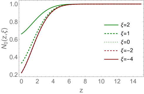
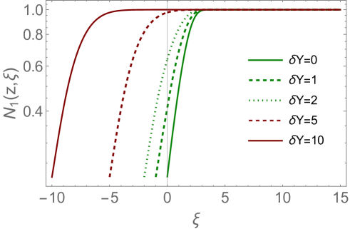
Fig. 2-a	Fig. 2-b

Figure 2: Fig. 2-a: $N_{0}(z,\xi)$ versus $z$ at fixed values of $\tilde{\xi}$. Fig. 2-b: $N_{0}(z,\xi)$ versus $\xi$ at fixed $\delta\tilde{Y}$ ($z=\kappa\delta\tilde{Y}+\xi$). $N_{0}=0.22;\\ \bar{\gamma}=0.63,\,\zeta-z_{0}=0.867,\,C_{1}=0.842,\,\xi^{A}_{0}=0$.

III.2 First iteration (linear in p)

For the first iteration, that takes into account the non-linear corrections we have the following equation for $M_{1}(\tilde{z},b,\delta\tilde{Y})$ (see Eq. (30):

$$\dfrac{\partial M_{1}}{\partial\delta\tilde{Y}}+\kappa\dfrac{\partial M_{1}}{\partial\tilde{z}}=\chi_{0}\left(\dfrac{\partial}{\partial\tilde{z}}\right)M_{1}-(\tilde{z}+\zeta)M_{1}\,-\,2\,\Phi_{1}\left(\delta\tilde{Y}\right)\,M_{0}-\dfrac{\partial A_{0}}{\partial\tilde{z}}$$ (72)

with $A_{0}(\tilde{z},\delta\tilde{Y},b)=\left(\int_{0}^{\tilde{z}}M_{0}(z^{\prime},\delta\tilde{Y})dz^{\prime}\right)^{2}$ (see Eq. (32)).

$M_{1}(\tilde{z},b,\delta\tilde{Y})$ is the solution to linear Eq. (72), which satisfies the following boundary and initial condition (see Fig. 1):

$$\mbox{region}\,I:\,\,M_{1}(\tilde{z}=\tilde{\xi}^{A}_{0})\,\,=\,\,0;~{}~{}~{}~{}\mbox{region}\,II:~{}~{}~{}M_{1}(\tilde{z},b,\delta\tilde{Y}=0)=\,\,0.$$ (73)

These boundaries and initial conditions show that both Eq. (7) at $z=\xi^{A}_{0}$ and Eq. (14) at $\delta\tilde{Y}=0$ have been satisfied by $N_{0}\left(\tilde{z},\delta\tilde{Y}\right)$.

III.2.1 $M^{I}_{1}\left(\tilde{z}\right)$ and $N^{I}_{1}\left(z\right)$

In the region I we are looking for the solution which is a function of $\boldsymbol{z}$. In addition we assume that $\Phi^{I}_{1}\left(\delta\tilde{Y}\right)=0$ Hence, the equation takes the form:

$$\kappa\dfrac{dM_{1}^{I}}{d\tilde{z}}\,=\,\chi_{0}\left(\dfrac{d}{d\tilde{z}}\right)M_{1}^{I}-(\tilde{z}+\zeta)M_{1}^{I}-\dfrac{dA_{0}^{I}}{d\tilde{z}},\quad\textrm{with}\quad\dfrac{dA_{0}^{I}}{d\tilde{z}}\,=\,2M_{0}^{I}\int_{0}^{\tilde{z}}M^{I}_{0}(z^{\prime})dz^{\prime}$$ (74)

Introducing $m_{1}^{I}(\gamma,\delta\tilde{Y})$ and $a_{0}^{I}(\gamma)$ such that

$$M_{1}^{I}(\tilde{z})\,=\,\int_{\epsilon-i\infty}^{\epsilon+i\infty}\dfrac{d\gamma}{2\pi i}e^{(\tilde{z}+\zeta)\gamma}m_{1}^{I}(\gamma,\delta\tilde{Y}),\quad\,\dfrac{dA_{0}^{I}}{d\tilde{z}}=\,\int_{\epsilon-i\infty}^{\epsilon+i\infty}\dfrac{d\gamma}{2\pi i}e^{(\tilde{z}+\zeta)\gamma}\,a_{0}(\gamma)$$ (75)

we reduce Eq. (74) to the form:

$$\dfrac{dm_{1}^{I}}{d\gamma}-\left(\kappa\gamma-\chi(\gamma)+\dfrac{1}{\gamma}\right)m_{1}^{I}\,=\,\,a_{0}(\gamma)$$ (76)

Using variation of parameter, one can see that the general solution of Eq. (76) looks as follows:

$$m_{1}^{I}(\gamma)\,=\,\left(C_{1}\,+\,\int_{0}^{\gamma}d\gamma^{\prime}\dfrac{a_{0}(\gamma^{\prime})}{m_{0}(\gamma^{\prime})}\right)\,m_{0}(\gamma)$$ (77)

In Eq. (77) the first term is a general solution of the homogeneous equation (see Eq. (43)) and the second one is the particular solution to the inhomogeneous equation. In Eq. (77) $C_{1}$ is chosen such that $M_{1}^{I}(\tilde{z}=\tilde{\xi}^{A}_{0})\,=\,0$.

Since

$$M_{1}^{I}(\tilde{z})\,=\,\dfrac{1}{2}\int_{0}^{\infty}dr^{\prime}\,J_{1}(r^{\prime}\,k_{\perp})N_{1}^{I}(r^{\prime})$$ (78)

and using the same procedure as for $M_{0}^{I}$ and $M_{0}^{II}$ we obtain

$$N_{1}^{I}(z)\,=\,2\,m(0)\,\int\limits_{\epsilon-i\infty}^{\epsilon+i\infty}\dfrac{d\gamma}{2\pi i}e^{(z+\zeta-z_{0})\gamma}\,e^{\frac{1}{2}\kappa\gamma^{2}}\left(C_{1}\,+\,\int_{0}^{\gamma}d\gamma^{\prime}\dfrac{a_{0}(\gamma^{\prime})}{m_{0}(\gamma^{\prime})}\right)$$ (79)

where

$$C_{1}\,=\,-\left(\int\limits_{\epsilon-i\infty}^{\epsilon+i\infty}\dfrac{d\gamma}{2\pi i}e^{(\xi^{A}_{0}\,+\,\zeta-z_{0})\gamma}\,e^{\frac{1}{2}\kappa\gamma^{2}}\,\int_{0}^{\gamma}d\gamma^{\prime}\dfrac{a_{0}(\gamma^{\prime})}{m_{0}(\gamma^{\prime})}\right)/\left(\int\limits_{\epsilon-i\infty}^{\epsilon+i\infty}\dfrac{d\gamma}{2\pi i}e^{(\xi_{0}^{A}+\zeta-z_{0})\gamma}\,e^{\frac{1}{2}\kappa\gamma^{2}}\right)$$ (80)

Finally, the solution takes the form

$$N^{I}_{1}\left(z\right)\,\,=\,\,C_{1}\left(N^{I}_{0}\left(z\right)\,-\,1\right)\,+\,\Delta^{I}_{1}\left(z\right)=\,\,C_{1}\left(N^{I}_{0}\left(z\right)\,\,-\,\,1\right)\,+\,\int\limits_{\epsilon-i\infty}^{\epsilon+i\infty}\dfrac{d\gamma}{2\pi i}e^{(z+\zeta-z_{0})\gamma}\,m(0)e^{\frac{1}{2}\kappa\gamma^{2}}\int_{0}^{\gamma}d\gamma^{\prime}\dfrac{a_{0}(\gamma^{\prime})}{m_{0}(\gamma^{\prime})}$$ (81)

whereas an estimative about their qualitative behavior (type of contribution) can be expressed as follows

$$N_{1}^{I}(z)\,\sim\,-\frac{c_{1}^{I}(\zeta)\,m(0)}{2\kappa\sqrt{2\pi\kappa}}\,(z-z_{0}^{A})\,\Delta_{01}(z)$$ (82)

with $c_{1}^{I}(\zeta)\,=\,-2\int\limits_{\epsilon-i\infty}^{\epsilon+i\infty}\frac{d\gamma}{2\pi i}\,\frac{d\gamma}{2\pi i}e^{\zeta\gamma}\frac{1}{\gamma}m_{0}^{I}(\gamma)$, being fulfilled $|N_{1}^{I}(z)|\ll N_{0}^{I}(z)$. See Appendix A for more details.

In our approach we have $\Delta_{01}(z)\,=\,e^{-\frac{1}{2\kappa}(z+\zeta-z_{0})^{2}}$, with $\dfrac{1}{\kappa}(\zeta-z_{0})\,=\,\frac{N_{0}}{(1-N_{0})}\,\overline{\gamma}$, see Eq. (66). Therefore, Eq. (82), can be rewritten as

$$N_{1}^{I}(z)\,\sim\,\exp\left(-\dfrac{z^{2}}{2\kappa}\right)\times\exp\left(-\left(\frac{N_{0}}{1-N_{0}}\right)\,\overline{\gamma}\,z\,+\,\ln(z-z_{0}^{A})\right)$$ (83)

with $\overline{\gamma}\,=\,1-\gamma_{cr}$.

III.2.2 $M_{1}^{II}(\tilde{z},\delta\tilde{Y})$ and $N_{1}^{II}(z,\delta\tilde{Y})$

In the region II the solution depends on two variables: $\tilde{z}$ and $\delta\tilde{Y}$. The term $\dfrac{\partial A^{II}_{0}}{\partial\tilde{z}}$ in the master equation has the form:

$$\dfrac{\partial A^{II}_{0}}{\partial\tilde{z}}\,=\,2M^{II}_{0}(\tilde{z},\delta\tilde{Y})\left(\lambda_{0}(\delta\tilde{Y})\,-\,\int_{\tilde{z}}^{\infty}d\tilde{z}^{\prime}M_{0}^{II}(\tilde{z}^{\prime},\delta\tilde{Y})\right)$$ (84)

where

$$\lambda_{0}(\delta\tilde{Y})\,=\,\int_{0}^{\kappa\delta\tilde{Y}}d\tilde{z}^{\prime}M_{0}^{I}(\tilde{z}^{\prime})\,+\,\int_{\kappa\delta\tilde{Y}}^{\infty}d\tilde{z}^{\prime}M^{II}_{0}(\tilde{z}^{\prime},\delta\tilde{Y})$$ (85)

Introducing the Mellin transforms for $m_{1}^{II}(\gamma,\delta\tilde{Y})$ and $a_{0}^{II}(\gamma,\delta\tilde{Y})$ such that

$$M_{1}^{II}(\tilde{z},\delta\tilde{Y})\,=\,\int_{\epsilon-i\infty}^{\epsilon+i\infty}\dfrac{d\gamma}{2\pi i}e^{(\tilde{z}+\zeta)\gamma}m_{1}^{II}(\gamma,\delta\tilde{Y}),\quad 2\,M_{0}^{II}(\tilde{z},\delta\tilde{Y})\int_{\tilde{z}}^{\infty}d\tilde{z}^{\prime}M^{II}_{0}(\tilde{z}^{\prime},\delta\tilde{Y})\,=\,\int_{\epsilon-i\infty}^{\epsilon+i\infty}\dfrac{d\gamma}{2\pi i}e^{(\tilde{z}+\zeta)\gamma}a_{0}^{II}(\gamma,\delta\tilde{Y})$$ (86)

Choosing $\Phi_{1}^{II}(\delta\tilde{Y})=-\lambda_{0}(\delta\tilde{Y})\,+\,\tilde{\Phi}_{1}^{(II)}\left(\delta\tilde{Y}\right)$ and repeating the same procedure as in Eq. (77), we reduce Eq. (72) to the form:

$$\dfrac{\partial m_{1}}{\partial\delta\tilde{Y}}+(\kappa\gamma-\chi(\gamma)+1/\gamma)m_{1}-\dfrac{\partial m_{1}}{\partial\gamma}\,+\,2\,\tilde{\Phi}^{(II)}_{1}\left(\delta\tilde{Y}\right)m_{0}=\,\,\,\,a^{II}_{0}(\gamma,\delta\tilde{Y})$$ (87)

In Eq. (86) we consider both $M_{1}\left(\tilde{z},\delta\tilde{Y}\right)$ and $A_{0}\left(\tilde{z},\delta\tilde{Y}\right)$ being equal to zero for negative $z$.

To solve Eq. (74) we introduce $m_{1}\left(\gamma,\delta\tilde{Y}\right)\,=\,-\,2\,\int\limits^{\delta\tilde{Y}}_{0}\!\!\!d\delta\tilde{Y}^{\prime}\tilde{\Phi}^{(II)}_{1}\left(\delta\tilde{Y}^{\prime}\right)m_{0}(\gamma,\delta\tilde{Y})+\tilde{m}_{1}\left(\gamma,\delta\tilde{Y}\right)$. Plugging this form of $m_{1}\left(\gamma,\tilde{Y}\right)$ in Eq. (78) we obtain

$$-\,2\,\int\limits^{\delta\tilde{Y}}_{0}\!\!\!d\delta\tilde{Y}^{\prime}\tilde{\Phi}^{(II)}_{1}\left(\delta\tilde{Y}^{\prime}\right)\underbrace{\Bigg{\{}\frac{\partial m^{II}_{0}\left(\gamma,\delta\tilde{Y}\right)}{\partial\delta\tilde{Y}}+(\kappa\gamma-\chi(\gamma)+1/\gamma)m^{II}_{0}\left(\gamma,\delta\tilde{Y}\right)-\dfrac{\partial m^{II}_{0}\left(\gamma,\delta\tilde{Y}\right)}{\partial\gamma}\Bigg{\}}}_{\mbox{ = 0 ( see {Eq.~{}(\ref{GSOL2})})}}$$

$$+\dfrac{\partial\tilde{m}_{1}}{\partial\delta\tilde{Y}}+(\kappa\gamma-\chi(\gamma)+1/\gamma)\tilde{m}_{1}-\dfrac{\partial\tilde{m}_{1}}{\partial\gamma}=\,\,\,\,a^{II}_{0}(\gamma,\delta\tilde{Y})$$ (88)

Searching a solution in the following form: $\tilde{m}_{1}\left(\gamma,\delta\tilde{Y}\right)\,\,=\,\,m_{0}(\gamma)\,\mu_{1}\left(\gamma,\delta\tilde{Y};b\right)$, we have for $\mu_{1}$:

$$m_{0}(\gamma)\Bigg{(}\dfrac{\partial\mu_{1}\left(\gamma,\delta\tilde{Y};b\right)}{\partial\tilde{Y}}\,\,-\,\,\dfrac{\partial\mu_{1}\left(\gamma,\delta\tilde{Y};b\right)}{\partial\gamma}\Bigg{)}\,-\,a^{II}_{0}(\gamma,\delta\tilde{Y})\,\,=\,\,0;~{}~{}~{}\dfrac{\partial\mu_{1}\left(\gamma,\tilde{Y};b\right)}{\partial\tilde{Y}}\,\,-\,\,\dfrac{\partial\mu_{1}\left(\gamma,\delta\tilde{Y};b\right)}{\partial\gamma}=\,\,\,\dfrac{a^{II}_{0}(\gamma,\delta\tilde{Y})}{m_{0}(\gamma)}$$ (89)

The solution to Eq. (89) can be found in the $\tilde{z}$ - representation, introducing

$$\tilde{\mu}_{1}\left(\tilde{z},\delta\tilde{Y}\right)\,\,=\,\,\int\limits^{\epsilon+i\infty}_{\epsilon-i\infty}\frac{d\gamma}{2\pi i}e^{\gamma\,\tilde{z}}\frac{\tilde{m}_{1}\left(\gamma,\delta\tilde{Y}\right)}{m_{0}\left(\gamma\right)};~{}~{}~{}~{}~{}~{}~{}\tilde{A}\left(\tilde{z},\delta\tilde{Y}\right)\,\,=\,\,\,\int\limits^{\epsilon+i\infty}_{\epsilon-i\infty}\frac{d\gamma}{2\pi i}e^{\gamma\,\tilde{z}}\frac{a^{II}_{0}\left(\gamma,\delta\tilde{Y}\right)}{m_{0}\left(\gamma\right)};$$ (90)

Eq. (89) takes the form

$$\frac{\partial\tilde{\mu}_{1}\left(\tilde{z},\delta\tilde{Y}\right)}{\partial\,\delta\tilde{Y}}\,\,+\,\,\tilde{z}\,\tilde{\mu}_{1}\left(\tilde{z},\delta\tilde{Y}\right)=\tilde{A}\left(\tilde{z},\delta\tilde{Y}\right)$$ (91)

The general solution to Eq. (91) can be found in the form: $\tilde{\mu}_{1}\left(\tilde{z},\delta\tilde{Y}\right)\,\,=\,\,e^{-\,\tilde{z}\,\delta\tilde{Y}}H\left(\tilde{z},\delta\tilde{Y}\right)$, with the following equation for $H$:

$$\frac{\partial H\left(\tilde{z},\delta\tilde{Y}\right)}{\partial\,\delta\tilde{Y}}=e^{\tilde{z}\,\delta\tilde{Y}}\tilde{A}\left(\tilde{z},\delta\tilde{Y}\right)$$ (92)

Finally, the solution, which satisfies the initial condition at $\delta\tilde{Y}=0$ (see Eq. (73)), has the form:

$$\tilde{\mu}_{1}\left(\tilde{z},\delta\tilde{Y}\right)=e^{-\tilde{z}\,\delta\tilde{Y}}\,\int\limits_{0}^{\delta\tilde{Y}}dte^{\tilde{z}t}\tilde{A}\left(\tilde{z},\,t\right)$$ (93)

For the Mellin image of $\tilde{\mu}_{1}\left(\tilde{z},\delta\tilde{Y}\right)$ we have:

$$\mu_{1}\left(\gamma,\delta\tilde{Y}\right)\,\,=\,\,\int\limits^{\delta\tilde{Y}}_{0}dt\frac{a^{II}_{0}\left(\gamma+\delta\tilde{Y}-t,t\right)}{m_{0}\left(\gamma+\delta\tilde{Y}-t\right)}$$ (94)

Hence, the general solution to Eq. (87), which satisfies the initial and boundary conditions of Eq. (73) takes the following form:

$$m^{(II)}_{1}\left(\gamma,\delta\tilde{Y}\right)\,\,=\,\,\,-\,2\,\int\limits^{\delta\tilde{Y}}_{0}\!\!dt\tilde{\Phi}^{II}_{1}\left(t\right)m_{0}(\gamma,\delta\tilde{Y})\,\,+\,\,m_{0}(\gamma)\int\limits^{\delta\tilde{Y}}_{0}dt\frac{a^{II}_{0}\left(\gamma+\delta\tilde{Y}-t,t\right)}{m_{0}\left(\gamma+\delta\tilde{Y}-t\right)}$$ (95)

The general solution for $N_{1}^{II}\left(r,\delta\tilde{Y}\right)$ has the following form

$$N^{II}_{1}\left(z,\delta\tilde{Y}\right)\,\,\,=\,\,\,\,2\,m(0)\int\limits^{\epsilon+i\infty}_{\epsilon-i\infty}\!\!\!\!\dfrac{d\,\gamma}{2\,\pi\,i}\,e^{(z+\zeta-z_{0})\,\gamma}e^{\frac{1}{2}\kappa\gamma^{2}}\,\int\limits^{\delta\tilde{Y}}_{0}dt\frac{a^{II}_{0}\left(\gamma+\delta\tilde{Y}-t,t\right)}{m_{0}\left(\gamma+\delta\tilde{Y}-t\right)}+I\left(z,\delta\tilde{Y}\right)$$ (96)

where $I\left(z,\delta\tilde{Y}\right)\,=\,-\,\int\limits^{\delta\tilde{Y}}_{0}d\delta\tilde{Y}^{\prime}\tilde{\Phi}^{II}_{1}\left(\delta\tilde{Y}^{\prime}\right)\Big{(}N^{II}_{0}\left(z,\delta\tilde{Y}\right)\,-\,1\Big{)}$. The developments for the analysis of the behavior of the contributions in Eq. (96) are presented in the appendix section, see Eq. (120). Our analysis led us to the following approximation

$$N_{1}^{II}(z,\delta\tilde{Y})\,=\,h(\delta Y)\,\exp\left(-\frac{1}{2}(z+\zeta-z_{0})\delta\tilde{Y}\right)\,\exp\left(-\frac{1}{2}(\xi+\zeta-z_{0})\delta\tilde{Y}\right)\,\exp\left(-\dfrac{r^{2}Q^{2}_{s}(Y_{A},b)}{4}\right)\,(1+o(1))$$ (97)

with $h(\delta\tilde{Y})\,=\,-\int_{0}^{\delta\tilde{Y}}d\delta\tilde{Y}^{\prime}\tilde{\Phi}_{1}^{II}(\delta\tilde{Y}^{\prime})$.

III.2.3 Matching at $\xi=\xi^{A}_{0}$

The matching condition at $\xi=\xi^{A}_{0}$ is

$$N^{I}_{1}\left(z\right)\,\,=\,\,N^{II}_{1}\left(z,\delta\tilde{Y}\right)~{}~{}~{}\mbox{for}~{}~{}~{}z=\kappa\,\delta\tilde{Y}+\xi^{A}_{0}$$ (98)

Plugging in Eq. (98) the solutions presented in Eq. (79) and Eq. (96) one can see that Eq. (98) takes the following form

$$N^{I}_{1}\left(z=\xi^{A}_{0}+\kappa\delta\tilde{Y}\right)\,\,=\,\,-2\,m(0)\,\int\limits^{\epsilon+i\infty}_{\epsilon-i\infty}\!\!\dfrac{d\,\gamma}{2\,\pi\,i}e^{(\xi^{A}_{0}+\kappa\delta\tilde{Y})\gamma}e^{\frac{1}{2}\kappa\,\gamma^{2}}\,\,\int\limits^{\delta\tilde{Y}}_{0}dt\frac{a^{II}_{0}\left(\gamma+\delta\tilde{Y}-t,t\right)}{m_{0}\left(\gamma+\delta\tilde{Y}-t\right)}\,+\,I\left(\xi^{A}_{0}+\kappa\delta\tilde{Y},\delta\tilde{Y}\right)$$ (99)

We need to recall, that $a_{0}(\gamma^{\prime},\delta\tilde{Y})$ has different forms for $M^{I}_{1}\left(\tilde{z}\right)$ and for $M^{II}_{1}\left(\tilde{z},\delta\tilde{Y}\right)$. For the region I $a^{I}_{0}(\gamma)$ it is a Mellin image of $2\,M^{I}_{0}\left(\tilde{z}\right)\int\limits^{\tilde{z}}_{0}d\tilde{z}^{\prime}\,M^{I}_{0}\left(\tilde{z}^{\prime}\right)$, while the region II $a^{II}_{0}(\gamma,\delta\tilde{Y})$ it is a Mellin image of Eq. (84) and Eq. (85). Actually the contribution of $M^{I}_{0}$ leads to the change of function $\Phi^{II}_{1}\left(\delta\tilde{Y}\right)$, and, therefore

$$a_{0}^{II}\left(\gamma,\delta\tilde{Y}\right)\,\,=\,\,\int\limits^{\infty}_{0}d\,\tilde{z}\,e^{-\gamma\,\tilde{z}}\,2\,M^{II}_{0}\left(\tilde{z},\delta\tilde{Y}\right)\,\,\int\limits^{z}_{\kappa\,\delta\tilde{Y}}d\tilde{z}^{\prime}\,M^{II}_{0}\left(\tilde{z}^{\prime},\delta\tilde{Y}\right)$$ (100)

Function $\Phi\left(\delta\tilde{Y}\right)$ has to be found from the following equation:

$$\int\limits^{\delta\tilde{Y}}_{0}d\delta\tilde{Y}^{\prime}\Phi^{II}_{1}\left(\delta\tilde{Y}^{\prime}\right)\Big{(}N^{II}_{0}\left(\xi^{A}_{0}+\kappa\delta\tilde{Y},\delta\tilde{Y}\right)\,-\,1\Big{)}=N^{I}_{1}\left(\xi^{A}_{0}+\kappa\,\delta\tilde{Y}\right)\,+\,2\,\int\limits^{\epsilon+i\infty}_{\epsilon-i\infty}\dfrac{d\,\gamma}{2\,\pi\,i}e^{(\xi^{A}_{0}+\kappa\delta\tilde{Y})\gamma}\,e^{\frac{1}{2}\kappa\,\gamma^{2}}\int\limits^{\delta\tilde{Y}}_{0}dt\frac{a^{II}_{0}\left(\gamma+\delta\tilde{Y}-t,t\right)}{m_{0}\left(\gamma+\delta\tilde{Y}-t\right)}$$ (101)

III.2.4 Numerical estimates

$N^{I}_{1}\left(z\right)$:

For numerical estimates we use Eq. (79) calculating the integral over $\gamma$ along the imaginary axis. The integral is concentrated in vicinity of small $\gamma$ due to the factor $\exp\left(-\frac{1}{2}\kappa\left({\rm Im}\,\gamma\right)^{2}\right)$. The second term in Eq. (79) can be rewritten in more convenient form for numerical estimates, viz.:

$$-2\!\!\int\limits^{\epsilon+i\infty}_{\epsilon-i\infty}\!\!\!\frac{d\gamma}{2\,\pi\,i}e^{(z+\zeta-z_{0})\,\gamma}e^{\frac{1}{2}\kappa\gamma^{2}}\,\int\limits^{\gamma}_{0}d\gamma^{\prime}\dfrac{a_{0}(\gamma^{\prime})}{m_{0}(\gamma^{\prime})}\,\,=\,\,-2\int\limits^{\infty}_{0}\!\frac{d\nu}{\pi}{\rm Re}\Bigg{(}e^{i(z+\zeta-z_{0})\,\nu}\,i\,\int^{\nu}_{0}\!\!\!dt\exp\left(-\frac{1}{2}\kappa\,\nu(2\nu-t)\right)a_{0}\left(\nu-t\right)\Bigg{)}$$ (102)

One can see from Eq. (102) that integral over $\nu$ is well converged at $\nu$ close to 0.

In Fig. 3-a we plot the numerical estimates of $N^{I}_{1}\left(z\right)$ for $\xi^{A}_{0}=0$. One can see that the value of $N^{I}_{1}$ turns out to be very small. Hence, we see that out homotopy approach leads to a regular way to take into account the non linear corrections. We can recall that our approach consists of two steps. First we solve the linearized version of the non linear evolution equation at large values of $z$ (see Ref.LT ). Second, we calculate the corrections to this solution, using the homotopy approach. The small values of $N^{I}_{1}$ shows that homotopy approach gives the efficient way to take into account the shadowing corrections.

$N^{II}_{1}\left(z,\delta\tilde{Y}\right)$:

In Fig. 3-b we plot the first correction to the scattering amplitude. It should be noted that we did not face any difficulties in estimating the integrals over $\gamma$ for $N^{II}_{1}\left(z,\delta Y\right)$, since the factor $\exp\left(+\frac{1}{2}\kappa\,\gamma^{2}\right)$ provides the good convergence of the integrals at our imaginary values of $\gamma$. This figure shows that at $z\leq\delta\tilde{Y}$ we have the geometric scaling behaviour of the scattering amplitude while for $z>\delta\tilde{Y}$ the amplitude started to depend on $\delta\tilde{Y}$ violating the geometric scaling behaviour.

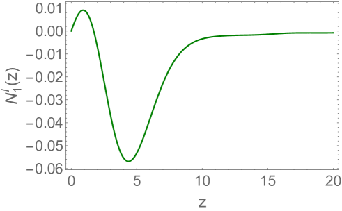
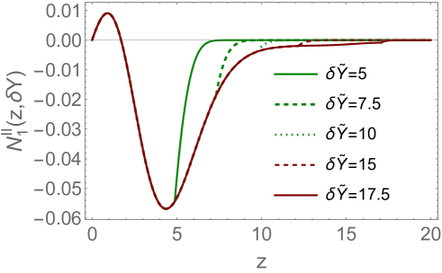
Fig. 3-a	Fig. 3-b

Figure 3: Fig. 3-a: $N^{I}_{1}\left(z\right)$ versus $z$. Fig. 3-b: $N_{1}\left(z,\delta Y\right)$ versus $z$ at fixed $\delta\tilde{Y}=\bar{\alpha}_{S}(Y-Y_{A})$. The value of $\xi^{A}_{0}=0$.

III.3 General case $p=n$

The general equation for $M_{n}$ has been written in Eq. (33) with $A_{n-1}$ defined in Eq. (32). The boundary and initial condition for all $M_{n}$ are the same as for $M_{1}$ and they are given by Eq. (73). In the same way as has been done in the first iteration, the analysis of the corrections should be developed in two different regions.

III.3.1 $M^{I}_{n}\left(\tilde{z}\right)$ and $N^{I}_{n}\left(z\right)$

Assuming $\Phi^{I}_{j}(\delta\tilde{Y})=0$ for $j\geq 1$, the contribution is obtained solving:

$$\kappa\,\dfrac{dM_{n}^{I}}{d\tilde{z}}\,=\,\chi_{0}\left(\dfrac{d}{d\tilde{z}}\right)M_{n}^{I}-(\tilde{z}-\zeta)\,M_{n}^{I}-\dfrac{dA_{n-1}^{I}}{d\tilde{z}},\quad\textrm{with}\,\dfrac{dA_{n-1}^{I}}{d\tilde{z}}\,=\,2\,\sum_{j=0}^{n-1}M^{I}_{j}(\tilde{z})\,\int_{0}^{\tilde{z}}M^{I}_{n-1-j}(z^{\prime})dz^{\prime}$$ (103)

Introducing Mellin transforms again

$$M_{n}^{I}(\tilde{z})\,=\,\int_{\epsilon-i\infty}^{\epsilon+i\infty}\dfrac{d\gamma}{2\pi i}\,e^{(\tilde{z}+\zeta)\gamma}\,m_{n}^{I}(\gamma),\quad\dfrac{dA_{n-1}}{d\tilde{z}}\,=\,\int_{\epsilon-i\infty}^{\epsilon+i\infty}\dfrac{d\gamma}{2\pi i}\,e^{(\tilde{z}+\zeta)\gamma}\,a_{n-1}^{I}(\gamma)$$ (104)

we obtain the ordinary differential equation for $m_{n}^{I}$ with the same structure as Eq. (76), with non homogeneous term $-a_{n-1}^{I}(\gamma)$, which depends recursively on the previous solutions.

Using a similar procedure as for $N_{1}^{I}(z)$ (see Appendix A), we obtain

$$\kappa\dfrac{dN_{n}^{I}}{d\tilde{z}}\,+\,(z+\zeta-z_{0})\,N_{n}^{I}\,=\,-\,\underbrace{\int_{\epsilon-i\infty}^{\epsilon+i\infty}\dfrac{d\gamma}{2\pi i}\,u^{-\gamma}e^{2\psi(1)\gamma}\,a_{n-1}^{I}(\gamma)\dfrac{\Gamma(1-\gamma)}{\Gamma(1+\gamma)}}_{H^{I}_{n}(z)}$$ (105)

where $u=e^{-(z+\zeta-z_{0})}$. Eq. (105) satisfies the condition $N_{n}^{I}(z_{0}^{A})\,=\,0$, with an approximate contribution given by

$$N_{n}^{I}(z)\,\sim\,-\frac{c_{n}^{I}(\zeta)\,m(0)}{2\kappa\sqrt{2\pi\kappa}}\,(z-z_{0}^{A})\,\Delta_{01}(z)$$ (106)

for some constant $c_{n}(\zeta)$ which depends on the previous solutions: $m_{j}^{I}(\gamma)$. As we discuss in the appendix, this contribution is small, confirming our numerical estimates.

III.3.2 $M^{II}_{n}\left(\tilde{z},\delta\tilde{Y}\right)$ and $N^{II}_{n}\left(z,\delta\tilde{Y}\right)$

The nonhomogeneous term takes the form:

$$\dfrac{\partial A^{II}_{n-1}}{\partial\tilde{z}}\,=\,2\sum_{j=0}^{n-1}\,M^{II}_{j}(\tilde{z},\delta\tilde{Y})\,\int_{0}^{\tilde{z}}d\tilde{z}^{\prime}\,M^{II}_{n-1-j}(\tilde{z}^{\prime},\delta\tilde{Y})$$ (107)

The differences in the expressions with respect to the regions are treated considering

$$\int_{0}^{\tilde{z}}d\tilde{z}^{\prime}\,M_{l}(\tilde{z}^{\prime},\delta\tilde{Y})\,=\,\lambda_{l}(\delta\tilde{Y})\,+\,\int_{\tilde{z}}^{\infty}d\tilde{z}^{\prime}M^{II}_{l}(\tilde{z}^{\prime},\delta\tilde{Y}),$$

with $\lambda_{l}(\delta\tilde{Y})\,=\,\int_{0}^{\infty}d\tilde{z}^{\prime}\,M_{l}(\tilde{z}^{\prime},\delta\tilde{Y})$. Writing $\Phi_{l+1}^{II}\,=\,-\,\lambda_{l}(\delta\tilde{Y})\,+\,\tilde{\Phi}_{l+1}^{II}(\delta\tilde{Y})$, we have

$$-2\sum_{j=0}^{n-1}\Phi_{n-j}^{II}(\delta\tilde{Y})\,M_{j}^{II}(\tilde{z},\delta\tilde{Y})\,-\,\dfrac{\partial A_{n-1}}{\partial\tilde{z}}\,=\,-2\,\sum_{j=0}^{n-1}\tilde{\Phi}_{n-j}^{II}(\delta\tilde{Y})\,M^{II}_{j}(\tilde{z},\delta\tilde{Y})\,+\,\underbrace{2\sum_{j=0}^{n-1}M_{j}^{II}(\tilde{z},\delta\tilde{Y})\,\int_{0}^{\tilde{z}}d\tilde{z}^{\prime}M^{II}_{n-1-j}(\tilde{z}^{\prime},\delta\tilde{Y})}_{\tilde{A}_{n-1}(\tilde{z},\delta\tilde{Y})}$$

Eq. (33) for the Mellin images takes the form:

$$\dfrac{\partial m_{n}\left(\gamma,\delta\tilde{Y}\right)}{\partial\delta\tilde{Y}}+(\kappa\gamma-\chi(\gamma)+1/\gamma)m_{n}\left(\gamma,\delta\tilde{Y}\right)-\dfrac{\partial m_{n}\left(\gamma,\delta\tilde{Y}\right)}{\partial\gamma}\,+\,2\,\sum_{j=0}^{n-1}\tilde{\Phi}^{II}_{n-j}\left(\delta\tilde{Y}\right)\,m_{j}\left(\gamma,\delta\tilde{Y}\right)=\,\,\,\,a_{n-1}^{II}(\gamma,\delta\tilde{Y})$$ (108)

where $\tilde{A}_{n-1}=\int_{\epsilon-i\infty}^{\epsilon+i\infty}\frac{d\gamma}{2\pi i}e^{(\tilde{z}+\zeta)\gamma}a_{n-1}^{II}(\gamma,\delta\tilde{Y})$.

Note, that for $n\geq 2$ we need to consider extra contributions in comparison with Eq. (III.2.2), since the solution for each $p=1,\dots,n-1$ satisfies a non-homogeneous equation. Thus, from the linearity of the equation, we can solve Eq. (108) considering a superposition of non-homegeneous contributions, i.e, $b_{n}(\gamma,\delta\tilde{Y})=-2\sum_{j=0}^{n-1}\tilde{\Phi}_{n-j}(\delta\tilde{Y})m_{j}(\gamma,\delta\tilde{Y})\,+\,a_{n-1}^{II}(\gamma,\delta\tilde{Y})$. Writing $m_{n}(\gamma,\delta\tilde{Y})\,=\,m_{0}(\gamma)\,\mu_{n}(\gamma,\delta\tilde{Y})$ we obtain the following equation for $\mu_{n}$:

$$\dfrac{\partial\mu_{n}\left(\gamma,\delta\tilde{Y}\right)}{\partial\delta\tilde{Y}}\,\,-\,\,\dfrac{\partial\mu_{n}\left(\gamma,\delta\tilde{Y}\right)}{\partial\gamma}=\,\,\,\dfrac{b_{n}(\gamma,\delta\tilde{Y})}{m_{0}(\gamma)}$$ (109)

Following similar procedure as in Eq. (96), we see that the solution in coordinate space has the form:

$$N^{II}_{n}\left(z,\delta\tilde{Y}\right)\,\,\,=\,\,\,\,2\,m(0)\int\limits^{\epsilon+i\infty}_{\epsilon-i\infty}\!\!\!\!\dfrac{d\,\gamma}{2\,\pi\,i}\,e^{(z+\zeta-z_{0})\,\gamma}e^{\frac{1}{2}\kappa\gamma^{2}}\,\int\limits^{\delta\tilde{Y}}_{0}dt\frac{b_{n}\left(\gamma+\delta\tilde{Y}-t,t\right)}{m_{0}\left(\gamma+\delta\tilde{Y}-t\right)}$$ (110)

Finally, plugging $b_{n}(\gamma,\delta\tilde{Y})=-2\sum_{j=0}^{n-1}\tilde{\Phi}_{n-j}(\delta\tilde{Y})m_{j}(\gamma,\delta\tilde{Y})\,+\,a_{n-1}^{II}(\gamma,\delta\tilde{Y})$ into Eq. (110) we obtain the integral representation of the solution from the recursive definition for each $m_{j}(\gamma,\delta\tilde{Y})$.

IV Conclusions

In this paper we developed the homotopy approach for solving the non-linear evolution Balitsky-Kovchegov equationBK . The solution consists of two steps. First, we solved the linearized version of the BK equation LT in the momentum space deep in the saturation region. We found that this solution has the geometric scaling behaviour for $\xi\leq\xi^{A}_{0}$ (see Fig. 1). For $\xi\,>\,\xi^{A}_{0}$, we observe the strong violation of the geometric scaling behaviour in the saturation region. This solution satisfies the boundary and initial conditions which are given perturbative QCD approach for $r\,Q_{s}<1$ (see Eq. (7)) and by McLerran-Venugopalan formula of Eq. (14) for $Y=Y_{A}$.

In the second step of our approach we are taking into account the remaining part of the non-linear correction that have not been included in the linearized form of BK equation. It turns out that these corrections are rather small indicating that our procedure gives a self consistent way to account them.

We believe that we suggest the method of finding solution, which allow us to treat the most essential part of the scattering amplitude analytically. The numerical part of the calculations is expressed through well converged integrals and can be easily estimated. However, in this paper we have not investigated the corrections $N^{I}\left(z\right)$ and $N^{II}\left(z,\delta\tilde{Y}\right)$ in full using that dependence of $z$ of ${A}_{0}(z,\delta\tilde{Y})$ is determined by the contribution of $M^{I}_{0}$ and $M^{II}_{0}$. These study would make the paper long and unreadable. Hence, we decided to put this in a separate paper with more mathematical content, which will be prepared shortly.

V Acknowledgements

We thank our colleagues at Tel Aviv University and UTFSM for encouraging discussions. CC thanks the department of particle physics of Tel Aviv University for hospitality and support during his stay. This research was supported by ANID PIA/APOYO AFB180002 (Chile) and Fondecyt (Chile) grant 1191434.

Appendix A Representations and qualitative aspects

In this appendix we collected our findings of analytical estimates of $N_{1}^{I}(z)$ and $N_{1}^{II}(z,\delta\tilde{Y})$. We believe that these estimates show that these functions are small and illustrate our main result: the practical approach to solution of the BK non-linear equation in which we can find analytically the main part of the solution leaving the small corrections to be treated numerically.

A.0.1 $N_{1}^{I}(z)$ in the geometrical scaling region

Introducing $N_{1}^{I}(z)\,=\,C_{1}^{I}\,(N^{I}_{0}(z)-1)\,+\,\Delta_{1}^{I}(z)$, with

$$\Delta_{1}^{I}(z)\,=\,\int_{\epsilon-i\infty}^{\epsilon+i\infty}\dfrac{d\gamma}{2\pi i}e^{(z+\zeta-z_{0})\gamma}\underbrace{m(0)e^{\frac{1}{2}\kappa\gamma^{2}}\int_{0}^{\gamma}d\gamma^{\prime}\dfrac{a_{0}(\gamma^{\prime})}{m_{0}(\gamma^{\prime})}}_{g_{1}(\gamma)}$$

and with $N_{0}^{I}(z)-1=C_{1}\,\Delta_{01}(z)$ where $C_{1}=-4m(0)/\sqrt{2\pi\kappa}$ and $\Delta_{01}(z)=e^{-\frac{(z+\zeta-z_{0})^{2}}{2\kappa}}$ is asymptotic formula of Ref.LT , we have $N_{1}^{I}(z)\,=\,\widetilde{C}_{1}\,\Delta_{01}(z)\,+\,\Delta_{1}^{I}(z)$ where $\widetilde{C}_{1}=-(\Delta_{1}^{I}(z^{A}_{0})/\Delta_{01}(z^{A}_{0}))$, with $z_{0}^{A}=\xi_{0}^{A}$.

From the equation for $g_{1}(\gamma)$:

$$\dfrac{dg_{1}}{d\gamma}\,=\,\kappa\gamma g_{1}\,+\,e^{2\psi(1)\gamma}\dfrac{\Gamma(1-\gamma)}{\Gamma(1+\gamma)}a_{0}^{I}(\gamma)$$

we can conclude

$$\kappa\dfrac{d\Delta_{1}^{I}}{dz}\,+\,(z+\zeta-z_{0})\Delta_{1}^{I}\,=\,-\,\underbrace{\int_{\epsilon-i\infty}^{\epsilon+i\infty}\dfrac{d\gamma}{2\pi i}\,u^{-\gamma}e^{2\psi(1)\gamma}\,a_{0}^{I}(\gamma)\dfrac{\Gamma(1-\gamma)}{\Gamma(1+\gamma)}}_{H^{I}_{1}(z)}$$

with $u=e^{-(z+\zeta-z_{0})}$. The solution to this equation has the form:

$$\Delta_{1}^{I}(z)\,=\,-\dfrac{1}{\kappa}\,\Delta_{01}(z)\int_{z_{0}^{A}}^{z}\dfrac{1}{\Delta_{01}(z^{\prime})}H_{1}^{I}(z^{\prime})\,dz^{\prime}\,+\,(\Delta_{1}^{I}(z^{A}_{0})/\Delta_{01}(z^{A}_{0}))$$

which leads us

$$N_{1}^{I}(z)\,=\,-\left(\dfrac{1}{\kappa}\int_{z_{0}^{A}}^{z}\dfrac{1}{\Delta_{01}(z^{\prime})}H_{1}^{I}(z^{\prime})\,dz^{\prime}\,\right)\,\Delta_{01}(z)$$ (111)

It is worthwhile mentioning that $N_{1}^{I}(z)$ satisfies

$$\dfrac{dN_{1}^{I}}{dz}+\dfrac{(z+\zeta-z_{0})}{\kappa}\,N_{1}^{I}\,=\,-\dfrac{1}{\kappa}H_{1}^{I}(z),$$ (112)

with leads to a general case of Eq. (105)). Note that $\Delta_{10}(z)$ is the homogeneous solution of Eq. (112).

On the other hands, the non-homogeneous term $H_{1}^{I}(z)$ can be expressed in term of convolution product between Mellin transforms (see formula 6.1.14 of Ref.BATEMAN ) as follows:

$$H_{1}^{I}(z)\,=\,e^{\psi(1)}e^{(z+\zeta-z_{0})/2}\,\int_{0}^{\infty}B_{0}^{I}(\eta)\,J_{1}\left(2\,e^{\psi(1)}e^{(z+\zeta-z_{0})/2}\sqrt{\eta}\right)\,\dfrac{d\eta}{\sqrt{\eta}}$$ (113)

with $B_{0}^{I}(u)=\frac{dA_{0}^{I}}{d\tilde{z}}$. Form Eq. (74) we have $B_{0}^{I}(u)=2\,M_{0}^{I}(\tilde{z})\,\int_{0}^{\tilde{z}}d\tilde{z}^{\prime\prime}\,M_{0}^{I}(\tilde{z}^{\prime\prime})$, where

$$\int_{0}^{\tilde{z}}d\tilde{z}^{\prime\prime}\,M_{0}^{I}(\tilde{z}^{\prime\prime})\,=\,\int_{\epsilon-i\infty}^{\epsilon+i\infty}\dfrac{d\gamma}{2\pi i}e^{(\tilde{z}+\zeta)\gamma}\dfrac{1}{\gamma}m_{0}^{I}(\gamma)\,-\,\int_{\epsilon-i\infty}^{\epsilon+i\infty}\dfrac{d\gamma}{2\pi i}e^{\zeta\gamma}\dfrac{1}{\gamma}m_{0}^{I}(\gamma)$$ (114)

Assuming that the principal contribution is given by the constant term in Eq. (114), we estimate Eq. (113) considering the following approximation

$$\widetilde{H}_{1}^{I}(z)\,=\,c_{1}^{I}(\zeta)\,e^{\psi(1)}e^{(z+\zeta-z_{0})/2}\,\int_{0}^{\infty}M_{0}^{I}(\tilde{z}^{\prime})J_{1}\left(2\,e^{\psi(1)}e^{(z+\zeta-z_{0})/2}\sqrt{\eta}\right)\,\dfrac{d\eta}{\sqrt{\eta}}$$

with $c_{1}^{I}(\zeta)=-\,2\,\int_{\epsilon-i\infty}^{\epsilon+i\infty}\frac{d\gamma}{2\pi i}e^{\zeta\gamma}\frac{1}{\gamma}m_{0}^{I}(\gamma)$, and $M^{I}_{0}(\tilde{z}^{\prime})\,=\,\int_{\epsilon-i\infty}^{\epsilon+i\infty}\frac{d\gamma}{2\pi i}\eta^{-\gamma}m_{0}^{I}(\gamma)$. Introducing $r^{\prime}=e^{(z+\zeta)/2}$ and $\eta^{\prime}=\sqrt{\eta}$, we can rewrite

$$\widetilde{H}_{1}^{I}(z)\,=\,c_{1}^{I}(\zeta)\,e^{(z+\zeta)/2}\,\int_{0}^{\infty}M_{0}^{I}(\tilde{z}^{\prime\prime})\,J_{1}\left(r^{\prime}\,\eta^{\prime}\right)\,d\eta^{\prime}$$ (115)

with $M_{1}^{I}(\tilde{z}^{\prime\prime})\,=\,\int_{\epsilon-i\infty}^{\epsilon+i\infty}\frac{d\gamma}{2\pi i}(\eta^{\prime})^{-2\gamma}m_{0}^{I}(\gamma)$. Taking $\gamma^{\prime}=2\gamma$ and changing the order of integration, Eq. (115) becomes

$$\widetilde{H}_{1}^{I}(z)\,=\,\frac{1}{2}c_{1}^{I}(\zeta)\,e^{(z+\zeta)/2}\,\int_{\epsilon^{\prime}-i\infty}^{\epsilon^{\prime}+i\infty}\dfrac{d\gamma^{\prime}}{2\pi i}\left(\int_{0}^{\infty}(\eta^{\prime})^{-\gamma^{\prime}}\,J_{1}\left(r^{\prime}\,\eta^{\prime}\right)\,d\eta^{\prime}\right)\,m_{0}^{I}\left(\frac{\gamma}{2}\right)$$

From formula 6.561.14 of Ref.RY follows

$$\widetilde{H}_{1}^{I}(z)\,=\,\frac{m(0)}{4}c_{1}^{I}(\zeta)\,\int_{\epsilon^{\prime}-i\infty}^{\epsilon^{\prime}+i\infty}\dfrac{d\gamma^{\prime}}{2\pi i}\left(\frac{r^{\prime}\,e^{-\psi(1)}}{2}\right)^{\gamma^{\prime}}\,e^{\frac{\kappa}{8}(\gamma^{\prime})^{2}}$$

with $r^{\prime}e^{-\psi(1)}/2\,=\,e^{(z+\zeta-z_{0})/2}$, and therefore (use 7.2.1 of Ref.BATEMAN ) we have

$$\widetilde{H}_{1}^{I}(z)\,=\,\frac{m(0)}{2\sqrt{2\pi\kappa}}c_{1}^{I}(\zeta)\,\Delta_{01}(z).$$ (116)

Plugging this approximation into Eq. (111) we obtain the following estimates:

$$N_{1}^{I}(z)\,=\,\left(\dfrac{c_{1}^{I}(\zeta)\,m(0)}{2\kappa\sqrt{2\pi\kappa}}\,(z-z_{0}^{A})\,+\,o(|z|)\right)\,\Delta_{01}(z)$$ (117)

where the corrections, which were incorporated in $o(|z|)$, are obtained from the analysis of the contribution given by the term

$$m(0)\,M_{0}^{I}(z)\,\int_{\epsilon-i\infty}^{\epsilon+i\infty}\dfrac{d\gamma}{2\pi i}\,e^{(z+\zeta-2\psi(1))\gamma}\,e^{\frac{\kappa}{2}\gamma^{2}}\dfrac{\Gamma(\gamma)}{\Gamma(1-\gamma)}\,=\,\dfrac{2m(0)}{\sqrt{2\pi\kappa}}\,M_{0}^{I}(z)\,\int_{0}^{\infty}e^{-\frac{1}{2\kappa}\ln^{2}(t^{\prime})}J_{0}\left(2\sqrt{\dfrac{u}{t}}\right)\,\dfrac{dt^{\prime}}{t^{\prime}}$$

with $u=e^{-(z+\zeta-z_{0})}$. The detailed analysis of these contributions we will publish in a separate paper in the nearest future. However, one can see that Eq. (117) leads to a contribution, which is proportional to $\Delta_{01}(z)$. Therefore, it is small at least at large $z$.

A.0.2 $N_{1}^{II}(z,\delta\tilde{Y})$ in the region II

Introducing $h_{1}(\delta\tilde{Y})\,=\,-\int_{0}^{\delta\tilde{Y}}dt\tilde{\Phi}_{1}^{II}(t)$ and $g(\gamma,\delta\tilde{Y})=2m(0)\,e^{\frac{1}{2}\kappa\gamma^{2}}\int_{0}^{\delta\tilde{Y}}dt\frac{a_{0}^{II}(\gamma+\delta\tilde{Y}-t,t)}{m_{0}(\gamma+\delta\tilde{Y}-t)}$ we write $N_{1}^{II}(z,\delta\tilde{Y})\,=\,h(\delta\tilde{Y})(N_{0}^{II}(z,\delta\tilde{Y})-1)\,+\,N_{1,p}(z,\delta\tilde{Y})$ with $N_{1,p}(z,\delta\tilde{Y})=\int_{\epsilon-i\infty}^{\epsilon+i\infty}\frac{d\gamma}{2\pi i}e^{(z+\zeta-z_{0})\gamma}g(\gamma,\delta\tilde{Y})$, where $g(\gamma,\delta\tilde{Y})$ satisfies

$$\dfrac{\partial g}{\partial\delta\tilde{Y}}-\dfrac{\partial g}{\partial\gamma}\,=\,-\kappa\,\gamma\,g\,+\,2e^{\psi(1)\gamma}\dfrac{\Gamma(1-\gamma)}{\Gamma(1+\gamma)}\,a_{0}^{II}(\gamma,\delta\tilde{Y})$$ (118)

For $H^{II}_{1}(z,\delta\tilde{Y})\,=\,2\,\int_{\epsilon-i\infty}^{\epsilon+i\infty}\frac{d\gamma}{2\pi i}u^{-\gamma}e^{2\psi(1)\gamma}a_{0}^{II}(\gamma,\delta\tilde{Y})$ with $u=e^{z+\zeta-z_{0}}$ Eq. (118) can be rewriiten as the following partial differential equation:

$$\dfrac{\partial N_{1,p}}{\partial\delta\tilde{Y}}\,+\,(z+\zeta-z_{0})\,N_{1,p}\,+\,\kappa\,\dfrac{\partial N_{1,p}}{\partial z}\,=\,H_{1}^{II}(z,\delta\tilde{Y})$$

or equivalently

$$\dfrac{\partial\mu_{1}^{II}}{\partial\delta\tilde{Y}}\,+\,\kappa\dfrac{\partial\mu_{1}^{II}}{\partial z}\,=\,\dfrac{1}{\Delta_{10}(z)}H_{1}^{II}(z,\delta\tilde{Y})$$ (119)

where $\mu_{1}^{II}(z,\delta\tilde{Y})\,=\,N_{1,p}(z,\delta\tilde{Y})/\Delta_{01}(z)$, with $\Delta_{01}(z)$ the solution of Ref.LT . From $N_{1}^{II}(z,\delta\tilde{Y}=0)=0$, the solution can be written as follows

$$N_{1}^{II}(z,\delta\tilde{Y})\,=\,h_{1}(\delta\tilde{Y})\,(N_{0}^{II}(z,\delta\tilde{Y})-1)\,+\,\Delta_{01}(z)\,\int_{0}^{\delta\tilde{Y}}\dfrac{H_{1}^{II}(z-\kappa\delta\tilde{Y}+\kappa t,t)}{\Delta_{01}(z-\kappa\delta\tilde{Y}+\kappa t)}\,dt$$ (120)

We can express $H_{1}^{II}(z,t)$ similarly to Eq. (113), as the following convolution product :

$$H_{1}^{II}(z,t)\,=\,2\,e^{\psi(1)}e^{(z+\zeta-z_{0})/2}\,\int_{0}^{\infty}B_{0}^{II}(\eta\,,\,t)\,J_{1}\left(2\,e^{\psi(1)}e^{(z+\zeta-z_{0})/2}\sqrt{\eta}\right)\,\dfrac{d\eta}{\sqrt{\eta}}$$ (121)

with $B_{0}^{II}(\eta,t)\,=\,M_{0}^{II}(z^{\prime},t)\,\int_{z^{\prime}}^{\infty}d\tilde{z}^{\prime\prime}M^{II}_{0}(\tilde{z}^{\prime\prime},t)$ (see Eq. (86)). For $\epsilon<0$, we have

$$B_{0}^{II}(\eta,t)\,=\,-\dfrac{1}{4}\,(f_{1}(t))^{2}\,\left(\int_{\epsilon-i\infty}^{\epsilon+i\infty}\dfrac{d\gamma}{2\pi i}\eta^{-\gamma}\dfrac{\Gamma(1+\gamma)}{\Gamma(1-\gamma)}\,\Gamma(-(\gamma+t))\right)\left(\int_{\epsilon-i\infty}^{\epsilon+i\infty}\dfrac{d\gamma^{\prime}}{2\pi i}\eta^{-\gamma^{\prime}}\dfrac{\Gamma(\gamma^{\prime})}{\Gamma(1-\gamma^{\prime})}\,\Gamma(-(\gamma^{\prime}+t))\right)$$ (122)

with $\eta=e^{(z^{\prime}-\kappa t)}$ (see the variable in the Mellin transform presented in Eq. (59)). Introducing $G(\eta,t)$ such that $B_{0}^{II}(\eta,t)\,=\,-\frac{1}{4}(f_{1}(t))^{2}\,G(\eta,t)$, grouping and using Eq. (121), we can rewrite the second term of Eq. (120) in the form:

$$\begin{array}[]{l}\Delta_{01}(z)\,\displaystyle{\int_{0}^{\delta\tilde{Y}}\dfrac{H_{1}^{II}(z-\kappa\delta\tilde{Y}+\kappa t,t)}{\Delta_{01}(z-\kappa\delta\tilde{Y}+\kappa t)}\,dt}\,=\,-\frac{1}{4}\exp\left(-\frac{1}{2}(z+\zeta-z_{0})\,\delta\tilde{Y}\right)\,\exp\left(-\frac{1}{2}(\xi+\zeta-z_{0})\delta\tilde{Y}\right)\times\\ \,e^{(\xi+\zeta)/2}\displaystyle{\left(\int_{0}^{\delta\tilde{Y}}\,f_{1}(t)\left(\dfrac{r^{2}Q^{2}_{s}(Y_{A},b)}{4}\right)^{t}\,e^{\kappa\,t/2}\left[\int_{0}^{\infty}G(\eta,t)\,J_{1}\left(r\,Q_{s}(Y_{A},b)\,e^{\kappa\,t/2}\,\sqrt{\eta}\right)\,\dfrac{d\eta}{\sqrt{\eta}}\right]\,dt\right)}\end{array}$$ (123)

From Eq. (123) we see that the second term in Eq. (120) is proportional to $\Delta_{01}(z)$ and, therefore, it is not larger than the first term in this equation. However, we expect from Eq. (62) that the factor in parentheses is rather small, being of the order of $\exp\left(-\dfrac{r^{2}Q^{2}_{s}(Y_{A},b)}{2}\right)$. Bearing this in mind we assume that the contribution of Eq. (123) is smaller than the first term in Eq. (120) and, therefore, we can trust Eq. (97). We are planning to give a more complete proof of this smallness in our further publications.

References

- (1) L. V. Gribov, E. M. Levin and M. G. Ryskin, Phys. Rep. 100 (1983) 1.
- (2) A. H. Mueller and J. Qiu, Nucl. Phys. B268 (1986) 427.
-
(3)
L. McLerran and R. Venugopalan,
Phys. Rev. D49 (1994) 2233, 3352; D50 (1994) 2225;
D53 (1996) 458;
D59 (1999) 09400. - (4) A. H. Mueller, Nucl. Phys. B 415, 373 (1994); Nucl. Phys. B 437 (1995) 107 [arXiv:hep-ph/9408245].
- (5) Y. V. Kovchegov and E. Levin, “Quantum chromodynamics at high energy,” Cambridge Monographs on Particle Physics, Nuclear Physics and Cosmology, Cambridge University Press, 2012 and references therein.
- (6) I. Balitsky, [arXiv:hep-ph/9509348]; Phys. Rev. D60, 014020 (1999) [arXiv:hep-ph/9812311]; Y. V. Kovchegov, Phys. Rev. D60, 034008 (1999), [arXiv:hep-ph/9901281].
- (7) J. Jalilian-Marian, A. Kovner, A. Leonidov and H. Weigert, Nucl. Phys. B 504, 415 (1997) [hep-ph/9701284]; J. Jalilian-Marian, A. Kovner, A. Leonidov and H. Weigert, Phys. Rev. D 59, 014014 (1998) [hep-ph/9706377 J. Jalilian-Marian, A. Kovner and H. Weigert, Phys. Rev. D 59, 014015 (1998) [hep-ph/9709432] A. Kovner, J. G. Milhano and H. Weigert, Phys. Rev. D62, 114005 (2000), [arXiv:hep-ph/0004014] ; E. Iancu, A. Leonidov and L. D. McLerran, Phys. Lett. B510, 133 (2001); [arXiv:hep-ph/0102009]; Nucl. Phys. A692, 583 (2001), [arXiv:hep-ph/0011241]; E. Ferreiro, E. Iancu, A. Leonidov and L. McLerran, Nucl. Phys. A703, 489 (2002), [arXiv:hep-ph/0109115]; H. Weigert, Nucl. Phys. A703, 823 (2002), [arXiv:hep-ph/0004044].
- (8) J. L. Albacete and C. Marquet, Prog. Part. Nucl. Phys. 76 (2014) 1 [arXiv:1401.4866 [hep-ph]].
- (9) E. Levin and K. Tuchin, Nucl. Phys. B 573 (2000) 833 [arXiv:hep-ph/9908317].
- (10) J. Bartels, E. Levin, Nucl. Phys. B387 (1992) 617-637.
- (11) A. M. Stasto, K. J. Golec-Biernat, J. Kwiecinski, Phys. Rev. Lett. 86 (2001) 596-599, [hep-ph/0007192];
- (12) E. Iancu, K. Itakura, L. McLerran, Nucl. Phys. A708 (2002) 327-352. [hep-ph/0203137]
- (13) A. H. Mueller and D. N. Triantafyllopoulos, Nucl. Phys. B640 (2002) 331 [arXiv:hep-ph/0205167]; D. N. Triantafyllopoulos, Nucl. Phys. B648 (2003) 293 [arXiv:hep-ph/0209121].
- (14) V. S. Fadin, E. A. Kuraev and L. N. Lipatov, Phys. Lett. B60, 50 (1975); E. A. Kuraev, L. N. Lipatov and V. S. Fadin, Sov. Phys. JETP 45, 199 (1977), [Zh. Eksp. Teor. Fiz.72,377(1977)]; I. I. Balitsky and L. N. Lipatov, Sov. J. Nucl. Phys. 28, 822 (1978), [Yad. Fiz.28,1597(1978)].
- (15) L. N. Lipatov, Sov. Phys. JETP 63, 904 (1986) [Zh. Eksp. Teor. Fiz. 90, 1536 (1986)].
- (16) K. J. Golec-Biernat and A. M. Stasto, Nucl. Phys. B 668 (2003), 345-363 [arXiv:hep-ph/0306279 [hep-ph]].
- (17) J. Berger and A. Stasto, Phys. Rev. D 83 (2011), 034015 [arXiv:1010.0671 [hep-ph]].
- (18) A. Kovner and U. A. Wiedemann, Phys. Rev. D 66, 051502 (2002) [hep-ph/0112140].
- (19) A. Kovner and U. A. Wiedemann, Phys. Rev. D 66, 034031 (2002) [hep-ph/0204277]; ,̇
- (20) A. Kovner and U. A. Wiedemann, Phys. Lett. B 551, 311 (2003) [hep-ph/0207335].
- (21) E. Ferreiro, E. Iancu, K. Itakura and L. McLerran, Nucl. Phys. A 710, 373 (2002) [hep-ph/0206241].
-
(22)
M. Froissart,
123 (1961) 1053;
A. Martin, “Scattering Theory: Unitarity, Analitysity and Crossing." Lecture Notes in Physics, Springer-Verlag, Berlin-Heidelberg-New-York, 1969. - (23) E. Iancu, K. Itakura and S. Munier, Phys. Lett. B 590, 199 (2004) [hep-ph/0310338].
- (24) S. Bondarenko, M. Kozlov, E. Levin, Nucl. Phys. A727 (2003) 139-178, [hep-ph/0305150] .
- (25) A. H. Rezaeian and I. Schmidt, Phys. Rev. D 88 (2013) 074016 [arXiv:1307.0825 [hep-ph]].
- (26) C. Contreras, E. Levin and I. Potashnikova, Nucl. Phys. A 948 (2016), 1-18 [arXiv:1508.02544 [hep-ph]].
- (27) J.H. He, Comput. Methods Appl. Mech. Engrg. 173 (1999) 257.
- (28) J.H. He, Int. J. Nonlinear Mech. 35 (2000) 37.
- (29) R. Saikia, P. Phukan and J. K. Sarma, [arXiv:2204.10111 [hep-ph]].
- (30) K. Golec-Biernat and M. Wsthoff, Phys. Rev. D 59, 014017 (1998).
- (31) E. Levin and K. Tuchin, Nucl. Phys. A 693, 787 (2001) [hep-ph/0101275].
- (32) A. Kormilitzin, E. Levin and S. Tapia, Nucl. Phys. A 872, 245-264 (2011) doi:10.1016/j.nuclphysa.2011.09.021 [arXiv:1106.3268 [hep-ph]].
- (33) C. Contreras, E. Levin and R. Meneses, JHEP 10, 138 (2014) doi:10.1007/JHEP10(2014)138 [arXiv:1406.1212 [hep-ph]].
- (34) Yu, V. Kovchegov, , Phys. Rev. D 61 (2000) 074018.
- (35) Harry Bateman, Tables of integral transforms, McGraw-Hill book company, inc. 1954.
- (36) S. Munier and R. B. Peschanski, Phys. Rev. D 69, 034008 (2004) [hep-ph/0310357]; Phys. Rev. Lett. 91, 232001 (2003) [hep-ph/0309177].
- (37) I. Gradstein and I. Ryzhik, "Tables of Series, Products, and Integrals", Fifth Edition, Academic Press, London, 1994.