Tell Model Where to Attend: Improving Interpretability of Aspect-Based Sentiment Classification via Small Explanation Annotations

Abstract

Gradient-based explanation methods play an important role in the field of interpreting complex deep neural networks for NLP models. However, the existing work has shown that the gradients of a model are unstable and easily manipulable, which impacts the model’s reliability largely. According to our preliminary analyses, we also find the interpretability of gradient-based methods is limited for complex tasks, such as aspect-based sentiment classification (ABSC). In this paper, we propose an Interpretation-Enhanced Gradient-based framework for ABSC via a small number of explanation annotations, namely IEGA. Particularly, we first calculate the word-level saliency map based on gradients to measure the importance of the words in the sentence towards the given aspect. Then, we design a gradient correction module to enhance the model’s attention on the correct parts (e.g., opinion words). Our model is model agnostic and task agnostic so that it can be integrated into the existing ABSC methods or other tasks. Comprehensive experimental results on four benchmark datasets show that our IEGA can improve not only the interpretability of the model but also the performance and robustness.

Index Terms—  Interpretability, aspect-based sentiment classification, gradient-based

1 Introduction

Interpreting complex deep neural networks to understand the reasoning behind the decision of NLP models has attached much attention [1, 2]. Understanding how such models work is an important research with wide applications such as deployment [3] and helping developers improve the quality of the models [4]. Recently, post-hoc explanation techniques have been widely used, categorized into black-box and white-box methods. In this paper, we improve upon the gradient-based explanation method [5, 6], which is one of the main methods in white-box models. Gradient-based explanation method calculates the word importance explainability by estimating the contribution of input sentence $x$ towards output $y$ [7, 8, 9]. It calculates the first derivative of $y$ with respect to $x$ to obtain the saliency map, which is a popular technique applicable to various deep learning models.

However, the existing literature has shown that the gradient-based model is easily manipulable [10] and unreliable [11]. Moreover, we also find that the gradient-based methods perform poorly on complex NLP tasks, such as aspect-based sentiment classification (ABSC). ABSC aims to judge the sentiment polarity of the given aspect in the sentence, which may contain multiple aspects whose sentiments may be opposite. For example, in the sentence "I can say that I am fully satisfied with the performance that the computer has supplied.", the user expresses a positive sentiment towards the aspect "performance" using the opinion words "satisfied" (Fig. 1). We can find that the BERT-SPC model focuses on the unrelated words (e.g., "say", "I", "of", "is") via the standard gradient. Here, we hope the model can capture the most relevant words (e.g., "satisfied", "disappointment") for predicting based on small additional explanation annotations because labeling the fine-grained opinions is expensive.

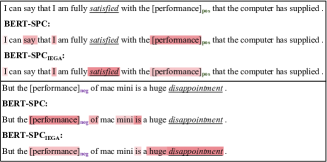
Fig. 1: Two examples of interpretability. The words marked with [] and underline are aspects and opinion words respectively. Pos and neg mean positive and negative sentiments of the aspects. Color depth indicates the importance of the words.

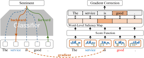
Fig. 2: The architecture of our IEGA proposed model.

Particularly, to enhance the model doing the "right thing”, we propose an Interpretation-Enhanced Grandient-based method (IEGA) for ABSC via small annotations. First, we use gradients to obtain the word-level saliency map, which measures the importance of the words for the predictions. Since labeling the opinion words toward the given aspects is time-consuming, we then aim to guide the model via small explainable annotations. Specifically, we design a gradient correction module to enforce the model to focus on the most related words (e.g., opinion words). We also conduct a series of experiments on four popular datasets for the ABSC task. The results indicate that our IEGA can improve not only the interpretability but also the performance of the model. Additionally, we also investigate the robustness of our model.

The main contributions of this paper can be summarized as follows. 1) We propose a novel framework to improve the interpretation of gradient-based methods for ABSC via a small number of additional explanation samples; 2) We design a gradient correction module to enable the model to capture the most related words based on the word-level saliency map; 3) We conduct extensive experiments to verify the great advantages of our IEGA framework, which can improve the explanation, performance, and robustness of the model.

2 Approaches

In this paper, we propose an IEGA framework for ABSC to enhance the interpretation of the model using small annotations (Fig. 2). First, we compute the gradients of $y$ with respect to $x$ based on a sentiment classifier. Second, we introduce a gradient correction module to make the word-level saliency map obtained by gradients close to the truth distributions of opinion words.

Formally, given a sentence $s=\{w_{1},...,w_{i},...,w_{|s|}\}$ and an aspect $a$, where aspect $a$ is a subsequence of $s$, $w_{i}$ is the $i$-th word in $s$, and $|s|$ is the number of the words in the sentence. The word embeddings of the sentence $s$ are $x=\{x_{1},...,x_{i},...,x_{|s|}\}$, where $x_{i}$ is the word embedding of $w_{i}$. This task aims to predict the sentiment polarity $y\in\{P,N,O\}$ of the sentence towards the given aspect $a$. $P$, $N$, $O$ represent positive, negative, and neutral, respectively. Moreover, we aim to explain the model by extracting the opinion words $o$ that express the sentiment w.r.t the aspect $a$.

2.1 Gradient Calculation

First, we train a sentiment classifier for ABSC, which aims to infer the sentiment of the sentence w.r.t. the given aspect. Let $\mathcal{F}$ be a sentiment classifier which predict the sentiment distribution $P(y|s,a)$ based on the sentence $s$ and aspect $a$.

$$P(y|s,a)=\mathcal{F}(s,a)$$ (1)

The loss function is the cross-entropy between the predicted probability and the true label,

$$\mathcal{L}_{c}(y,s,a)=-{\log P(y|s,a)}.$$ (2)

Particularly, the sentiment classifier $\mathcal{F}$ can be any existing aspect-level sentiment classifier models, such as BERT-SPC [12], RGAT-BERT [13].

If we slightly perturb the word $w_{i}$’s embedding $\mathbf{x_{i}}$ to $\mathbf{x_{i}}^{\prime}$ with $\|\mathbf{x_{i}}^{\prime}-\mathbf{x_{i}}\|\leq\varepsilon$, we can use the first-order approximation of $\mathcal{L}_{c}(y,s,a)_{\mathbf{x_{i}}}$ to compute the absolute change of the loss function, which indicates the importance of the word $w_{i}$. rl & |L_c(y, s, a)_x_i’ - L_c(y, s, a)_x_i|
≈|∇_x_iL_c(y, s, a)_x_i)^T (x_i’ - x_i)|
≤∥∇_x_iL_c(y, s, a)_x_i∥ ∥x_i’ - x_i∥
≤ε∥∇_x_iL_c(y, s, a)_x_i∥.

Thus, it is a natural approximation to metric what tokens are most relevant for a prediction using the gradient [5, 14]. The gradient of the $i$-th word $w_{i}$ is calculated as follows:

$$g_{i}=\nabla_{\mathbf{x_{i}}}\mathcal{L}_{c}(y,s,a)_{\mathbf{x_{i}}}=\frac{\partial\mathcal{F}\left(s,a\right)}{\partial x_{i}}$$ (3)

which can be computed automatically via machine learning frameworks, such as Pytorch and Tensorflow.

2.2 Gradient Correction

In order to enhance the model to focus on the correct parts (e.g., opinion words), we introduce a gradient correction module. We first calculate the importance of the words in the sentence based on the gradients to obtain the word-level saliency map. The magnitude of the gradient’s norm $\|g_{i}\|$ could be a sign of how sensitive the sentiment label is to $w_{i}$: to get the correct prediction we will prefer not to perturb those words with large gradient norms. It suggests that words with large gradient norm are contributing most towards the correct sentiment label and might be the opinion words of the aspect. Thus, we define the attribution for the word $w_{i}$ as

$$\alpha_{i}=\frac{\mathrm{score}(w_{i})}{\sum_{j}(\mathrm{score}(w_{j}))},$$

where $\mathrm{score}(w_{i})=\left|g_{i}\cdot x_{i}\right|$ converts the word gradients into weights by the dot product of the gradient $g_{i}$ and word embedding $x_{i}$. Gradients (of the output with respect to the input) are a natural analog of the model coefficients for a deep network. Therefore the product of the gradient and feature values is a proper importance score function [5, 14].

We use small labeled samples to make the word-level saliency map close to the distributions of opinion words.

$$\mathcal{L}_{g}=-\sum_{j=1}^{|s|}y^{o}_{j}\alpha_{j}$$ (4)

where $y^{o}_{j}=1$ if word $w_{j}$ is opinion word, else $y^{o}_{j}=0$.

Finally, we add the classification loss $\mathcal{L}_{c}$ and gradient correction loss $\mathcal{L}_{g}$ with a weight $\lambda$, $\mathcal{L}=\mathcal{L}_{c}+\lambda\mathcal{L}_{g}$.

3 Experiments

3.1 Experimental Setups

Datasets. To verify the effectiveness of IEGA, we conduct extensive experiments on four typical datasets: Res14, Lap14, Res15, and Res16 [15]. We follow the setting of [15], which labeled the opinion words for each aspect.

Metrics. To assess the models’ performance, we use two popular metrics, Accuracy and Macro-F1. To investigate the faithfulness of explanations, follow [10], we used Mean Reciprocal Rank (MRR) and Hit Rate (HR) to verify whether opinion words get higher scores in attribution. We also adopt the area over the perturbation curve (AOPC) [16, 17] and Post-hoc Accuracy (Ph-Acc) [18], which are widely used for explanations [19]. AOPC calculates the average change of accuracy over test data by deleting top $K$ words via the word-level saliency map. For Post-hoc Accuracy, we select the top $K$ words based on their importance weights as input to make a prediction and compare it with the ground truth. We set $K=5$ value in our experiments.

Baselines. We select four state-of-the-art baselines for aspect-based sentiment classification to investigate the performance: BERT-SPC [12], AEN-BERT [20], LCF-BERT [21], RGAT-BERT [13]. For the limitation of space, please see more details about the baselines on the original papers.

Implementation Details. While conducting our experiments, we adopt the BERT base as the pre-trained model of our sentiment classifier. Some hyperparameters like batch size, maximum epochs, and learning rate are set to 32, 20, and 2e-5. The weight $\lambda$ of gradient correction loss is fixed at 0.01.

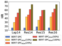
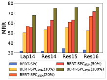
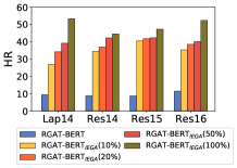
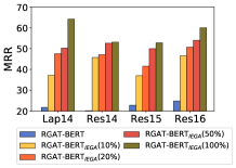
Fig. 3: The results of interpretability.

Table 1: The results of interpretability in terms of AOPC and Post-hoc Acc.

4 Model	Lap14		Res14		Res15		Res16
	AOPC$\uparrow$	Ph Acc$\uparrow$	AOPC$\uparrow$	Ph Acc$\uparrow$	AOPC$\uparrow$	Ph Acc$\uparrow$	AOPC$\uparrow$	Ph Acc$\uparrow$
BERT-SPC	07.24	33.70	07.95	56.87	06.50	64.84	03.82	65.44
BERT-SPC${}_{\texttt{IEGA}}$ (10%)	15.04(+7.80)	42.18(+8.48)	11.13(+3.18)	69.18(+12.31)	08.26(+1.76)	70.78(+5.94)	10.48(+6.66)	75.49(+10.05)
BERT-SPC${}_{\texttt{IEGA}}$ (20%)	18.54(+11.30)	42.38(+8.68)	12.35(+4.40)	74.17(+17.30)	09.65(+3.15)	71.98(+7.14)	11.49(+7.67)	76.27(+10.83)
BERT-SPC${}_{\texttt{IEGA}}$ (50%)	18.57(+11.33)	55.67(+21.97)	16.78(+8.83)	75.29(+18.42)	10.50(+4.00)	73.50(+8.66)	12.41(+8.59)	78.17(+12.73)
BERT-SPC${}_{\texttt{IEGA}}$ (100%)	21.90(+14.66)	59.73(+26.03)	20.47(+12.52)	76.12(+19.25)	11.98(+5.48)	74.65(+9.81)	15.87(+12.05)	79.82(+14.38)
RGAT-BERT	05.28	54.38	12.70	51.64	08.06	64.51	08.31	71.05
RGAT-BERT${}_{\texttt{IEGA}}$ (10%)	13.58(+8.30)	66.52(+12.14)	15.67(+2.97)	63.29(+11.65)	16.07(+8.01)	72.98(+8.47)	12.71(+4.40)	80.04(+8.99)
RGAT-BERT${}_{\texttt{IEGA}}$ (20%)	13.92(+8.64)	67.89(+13.51)	15.88(+3.18)	68.82(+17.18)	17.97(+9.91)	77.89(+13.38)	12.80(+4.49)	80.70(+9.65)
RGAT-BERT${}_{\texttt{IEGA}}$ (50%)	14.56(+9.28)	72.59(+18.21)	16.23(+3.53)	73.29(+21.65)	21.65(+13.59)	81.33(+16.82)	12.94(+4.63)	83.11(+12.06)
RGAT-BERT${}_{\texttt{IEGA}}$ (100%)	16.49(+11.21)	72.80(+18.42)	16.25(+3.55)	75.65(+24.01)	23.50(+15.44)	82.95(+18.44)	13.60(+5.29)	85.09(+14.04)
4

3.2 Experimental Analysis

Interpretability Analysis. We apply our IEGA framework to two classical ABSC models to explore the explanations of the models with different proportions of labeled opinion words (Fig. 3 and Table 1). The results show that our model captures the explanations (opinion words) more accurately. For example, both BERT-SPC${}_{\texttt{IEGA}}$ and RGAT-BERT${}_{\texttt{IEGA}}$ obtain higher HR and MRR, which indicates that they find opinion words more effectively than the corresponding models without IEGA. This is because the model can better capture the opinion words corresponding to the aspect with the help of gradient correction. For Post-hoc Accuracy, we compute the accuracy by selecting the top $5$ words based on their importance weights to make a prediction. Our model gains an increase of five points over all datasets in terms of Post-hoc Accuracy using only 10% (about 150) training samples annotated with opinion words. Also, models with IEGA perform better than ones without IEGA in terms of AOPC despite only partial training samples labeled opinion words. In summary, the improvement of these metrics shows that the interpretability of the model can be largely boosted with the help of our IEGA framework even if only 10% of the opinion words are annotated.

Table 2: Performance of our models and baselines.

4 Model	Lap14		Res14		Res15		Res16
	Acc.	F1	Acc.	F1	Acc.	F1	Acc.	F1
AEN-BERT	81.80	56.07	88.59	64.90	86.44	63.73	88.60	65.06
LCF-BERT	81.83	58.23	90.00	72.69	85.94	67.53	89.91	69.98
BERT-SPC	81.07	62.84	89.34	67.91	85.02	56.44	88.02	56.23
RGAT-BERT	82.58	65.10	91.64	77.50	87.09	69.36	90.78	67.34
BERT-SPC${}_{\texttt{IEGA}}$	82.28	62.93	90.62	72.75	85.40	59.39	88.56	62.60
Improvement	(+1.21)	(+0.09)	(+1.28)	(+4.84)	(+0.38)	(+2.95)	(+0.54)	(+6.37)
RGAT-BERT${}_{\texttt{IEGA}}$	83.08	65.56	92.36	79.30	88.25	72.49	91.76	76.02
Improvement	(+0.50)	(+0.46)	(+0.72)	(+1.80)	(+1.17)	(+3.13)	(+0.98)	(+8.68)
4

Performance Analysis. We compare our models with several ABSC models to evaluate the performance of our framework (Table 2). From the results, we obtain the following observations. First, our model performs better than the baselines over all the datasets in terms of accuracy and F1. RGAT-BERT${}_{\texttt{IEGA}}$ obtains the best results compared with all the existing state-of-the-art baselines (e.g., RGAT-BERT). Second, our IEGA framework can improve the performance of the base model. For instance, F1 improved by 3 and 8 points on Res15 and Res16 by integrating IEGA with RGAT-BERT.

Table 3: The results of robustness analysis.

4	Model	AddDiff		RevNon
		Acc.	F1	Acc.	F1
Lap14	BERT-SPC	45.21	32.01	50.20	41.61
	BERT-SPC${}_{\texttt{IEGA}}$	48.74	35.81	52.47	44.47
Res14	BERT-SPC	64.84	50.98	62.44	41.61
	BERT-SPC${}_{\texttt{IEGA}}$	67.10	52.28	66.03	58.16
Res15	BERT-SPC	46.38	33.38	56.58	38.45
	BERT-SPC${}_{\texttt{IEGA}}$	53.26	39.22	58.00	40.94
Res16	BERT-SPC	43.04	36.57	56.95	43.05
	BERT-SPC${}_{\texttt{IEGA}}$	52.19	39.68	59.07	43.60
4

Robustness Analysis. We also analyze the robustness of our proposed IEGA framework (Table 3). We test our model on two robustness testing datasets released by TextFlint [22]. RevNon reverses the sentiment of the non-target aspects with originally the same sentiment as the target aspect’s, and AddDiff adds a new non-target aspect whose sentiment is opposite to the target aspect of the sentence. We find that BERT-SPC${}_{\texttt{IEGA}}$ outperforms BERT-SPC over all datasets in terms of accuracy and F1. It shows that the model infers the sentiment based on the opinion words w.r.t the aspect stably. These observations suggest that our framework does have a large improvement in the robustness of the model.

4 Related Work

Gradient-based Analysis Models. Recently, studies on explanation methods has grown, including perturbation-based [3], gradient-based [23] and visualization-based [24] methods. We focus on the gradient-based method [5], a popular algorithm applicable to different neural network models. Gradient-based methods [25] have been widely applied into CV and NLP [24, 26]. The gradient-based approach is also used to understand the predictions of the text classification models from the token level [27, 28]. In addition, Rei et al. [29] adopted a gradient-based approach to detect the critical tokens in the sentence via the sentence-level label. The existing work also found that the gradient-based models are easily manipulable [10] and unreliable [11]. In this paper, we design an IEGA algorithm to force the model to discover the target-aware opinion words using the gradient.

Aspect-based Sentiment Classification. In recent years, thanks to the introduction of pre-trained language models, it has made tremendous progress in many NLP tasks, including aspect-based sentiment classification (ABSC) [30]. By simply connecting the aspect words with the original sentence and then inputting them into BERT for training, researchers obtain excellent results in ABSC tasks [12]. Furthermore, Song et al.[20] proposed AEN-BERT, which adopts attention-based encoders to model the interaction between context and aspect. Zeng et al. [21] proposed LCF-BERT, which uses multi-head self-attention to make the model focus on the local context words. Wang et al. [13] proposed a relation-aware graph attention network to model the tree structure knowledge for sentiment classification. However, most of them focus on improving performance, while the explanation of ABSC is not well studied. Yadav et al. [31] proposed a human-interpretable learning approach for ABSC, but there is still a big gap in accuracy compared to the state-of-the-art methods.

5 Conclusions and Future Work

In this paper, we introduce an IEGA framework to improve the explanations of the gradient-based methods for ABSC. We design a gradient correction algorithm based on the word-level saliency map via a tiny amount of labeled samples. We conduct extensive experimental results with various metrics over four popular datasets to verify the interpretation, performance, and robustness of the models using our IEGA. We also explore the influence of sample numbers and find that our framework can effectively improve the interpretation with small samples. It would be interesting to explore the performance of our model on more existing methods and tasks because IEGA is model agnostic and task agnostic.

References

- [1] Marina Danilevsky, Kun Qian, Ranit Aharonov, Yannis Katsis, Ban Kawas, and Prithviraj Sen, “A survey of the state of explainable AI for natural language processing,” in Proceedings of AACL, 2020.
- [2] Jie Zhou, Yuanbin Wu, Qin Chen, Xuan-Jing Huang, and Liang He, “Attending via both fine-tuning and compressing,” in Proceedings of ACL, 2021, pp. 2152–2161.
- [3] Marco Tulio Ribeiro, Sameer Singh, and Carlos Guestrin, “" why should i trust you?" explaining the predictions of any classifier,” in Proceedings of SIGKDD, 2016, pp. 1135–1144.
- [4] Eric Wallace, Jens Tuyls, Junlin Wang, Sanjay Subramanian, Matt Gardner, and Sameer Singh, “Allennlp interpret: A framework for explaining predictions of nlp models,” in Proceedings of EMNLP, 2019, pp. 7–12.
- [5] Karen Simonyan, Andrea Vedaldi, and Andrew Zisserman, “Deep inside convolutional networks: Visualising image classification models and saliency maps,” in Proceedings of ICLR, 2014.
- [6] Mukund Sundararajan, Ankur Taly, and Qiqi Yan, “Axiomatic attribution for deep networks,” in Proceedings of ICML, 2017, pp. 3319–3328.
- [7] Malika Aubakirova and Mohit Bansal, “Interpreting neural networks to improve politeness comprehension,” in Proceedings of EMNLP, 2016, pp. 2035–2041.
- [8] Sweta Karlekar, Tong Niu, and Mohit Bansal, “Detecting linguistic characteristics of alzheimer’s dementia by interpreting neural models,” in Proceedings of NAACL, 2018, pp. 701–707.
- [9] Jie Zhou, Yuanbin Wu, Changzhi Sun, and Liang He, “Is “hot pizza” positive or negative? mining target-aware sentiment lexicons,” in Proceedings of EACL, 2021, pp. 608–618.
- [10] Junlin Wang, Jens Tuyls, Eric Wallace, and Sameer Singh, “Gradient-based analysis of nlp models is manipulable,” in Proceedings of EMNLP, 2020, pp. 247–258.
- [11] Pieter-Jan Kindermans, Sara Hooker, Julius Adebayo, Maximilian Alber, Kristof T Schütt, Sven Dähne, Dumitru Erhan, and Been Kim, “The (un) reliability of saliency methods,” in Explainable AI: Interpreting, Explaining and Visualizing Deep Learning, pp. 267–280. Springer, 2019.
- [12] Hu Xu, Bing Liu, Lei Shu, and Philip Yu, “BERT post-training for review reading comprehension and aspect-based sentiment analysis,” in Proceedings of NAACL, 2019, pp. 2324–2335.
- [13] Kai Wang, Weizhou Shen, Yunyi Yang, Xiaojun Quan, and Rui Wang, “Relational graph attention network for aspect-based sentiment analysis,” in Proceedings of ACL, 2020, pp. 3229–3238.
- [14] David Baehrens, Timon Schroeter, Stefan Harmeling, Motoaki Kawanabe, Katja Hansen, and Klaus-Robert Müller, “How to explain individual classification decisions,” JMLR, vol. 11, pp. 1803–1831, 2010.
- [15] Zhifang Fan, Zhen Wu, Xin-Yu Dai, Shujian Huang, and Jiajun Chen, “Target-oriented opinion words extraction with target-fused neural sequence labeling,” in Proceedings of NAACL, June 2019, pp. 2509–2518.
- [16] Dong Nguyen, “Comparing automatic and human evaluation of local explanations for text classification,” in Proceedings of NAACL, 2018, pp. 1069–1078.
- [17] Wojciech Samek, Alexander Binder, Grégoire Montavon, Sebastian Lapuschkin, and Klaus-Robert Müller, “Evaluating the visualization of what a deep neural network has learned,” IEEE TNNLS, vol. 28, no. 11, pp. 2660–2673, 2016.
- [18] Jianbo Chen, Le Song, Martin Wainwright, and Michael Jordan, “Learning to explain: An information-theoretic perspective on model interpretation,” in Proceedings of ICML, 10–15 Jul 2018, vol. 80, pp. 883–892.
- [19] Hanjie Chen and Yangfeng Ji, “Learning variational word masks to improve the interpretability of neural text classifiers,” in Proceedings of EMNLP, 2020, pp. 4236–4251.
- [20] Youwei Song, Jiahai Wang, Tao Jiang, Zhiyue Liu, and Yanghui Rao, “Attentional encoder network for targeted sentiment classification,” arXiv preprint arXiv:1902.09314, 2019.
- [21] Biqing Zeng, Heng Yang, Ruyang Xu, Wu Zhou, and Xuli Han, “Lcf: A local context focus mechanism for aspect-based sentiment classification,” Applied Sciences, vol. 9, no. 16, pp. 3389, 2019.
- [22] Xiao Wang, Qin Liu, Tao Gui, Qi Zhang, Yicheng Zou, Xin Zhou, Jiacheng Ye, Yongxin Zhang, Rui Zheng, Zexiong Pang, et al., “Textflint: Unified multilingual robustness evaluation toolkit for natural language processing,” in Proceedings of ACL, 2021, pp. 347–355.
- [23] Alexander Binder, Grégoire Montavon, Sebastian Lapuschkin, Klaus-Robert Müller, and Wojciech Samek, “Layer-wise relevance propagation for neural networks with local renormalization layers,” in Proceedings of ICANN, 2016, pp. 63–71.
- [24] Matthew D. Zeiler and Rob Fergus, “Visualizing and understanding convolutional networks,” in ECCV, 2014, vol. 8689 of Lecture Notes in Computer Science, pp. 818–833.
- [25] Ian J. Goodfellow, Jonathon Shlens, and Christian Szegedy, “Explaining and harnessing adversarial examples,” in Proceedings of ICLR, 2015.
- [26] Bin Liang, Hongcheng Li, Miaoqiang Su, Pan Bian, Xirong Li, and Wenchang Shi, “Deep text classification can be fooled,” in Proceedings of IJCAI, 2018, pp. 4208–4215.
- [27] Jiwei Li, Xinlei Chen, Eduard H. Hovy, and Dan Jurafsky, “Visualizing and understanding neural models in NLP,” in Proceedings of NAACL, 2016, pp. 681–691.
- [28] Dimitrios Alikaniotis, Helen Yannakoudakis, and Marek Rei, “Automatic text scoring using neural networks,” in Proceedings of ACL, 2016.
- [29] Marek Rei and Anders Søgaard, “Zero-shot sequence labeling: Transferring knowledge from sentences to tokens,” in Proceedings of NAACL, 2018, pp. 293–302.
- [30] Jie Zhou, Jimmy Xiangji Huang, Qin Chen, Qinmin Vivian Hu, Tingting Wang, and Liang He, “Deep learning for aspect-level sentiment classification: survey, vision, and challenges,” IEEE access, vol. 7, pp. 78454–78483, 2019.
- [31] Rohan K Yadav, Lei Jiao, Ole-Christoffer Granmo, and Morten Goodwin, “Human-level interpretable learning for aspect-based sentiment analysis,” in Proceedings of AAAI, 2021, vol. 35, pp. 14203–14212.