Data-based Adaptive Refinement of Finite Element Thin Plate Spline

Abstract

The thin plate spline, as introduced by Duchon, interpolates a smooth surface through scattered data. It is computationally expensive when there are many data points. The finite element thin plate spline (TPSFEM) possesses similar smoothing properties and is efficient for large data sets. Its efficiency is further improved by adaptive refinement that adapts the precision of the finite element grid. Adaptive refinement processes and error indicators developed for partial differential equations may not apply to the TPSFEM as it incorporates information about the scattered data. This additional information results in features not evident in partial differential equations. An iterative adaptive refinement process and five error indicators were adapted for the TPSFEM. We give comprehensive depictions of the process in this article and evaluate the error indicators through a numerical experiment with a model problem and two bathymetric surveys in square and L-shaped domains.

1 Introduction

Scattered data from real-world applications often consist of noise-perturbed data points that need to be modelled and analysed [1]. The finite element thin plate spline (TPSFEM) combines the favourable properties of the thin plate spline (TPS) and finite element surface fitting, which allows it to approximate and smooth large data sets efficiently [2]. The accuracy of the TPSFEM is improved by iteratively refining its finite element grid, and the efficiency is further enhanced by using adaptive refinement that only refines certain sensitive regions marked by error indicators [3]. To construct the error indicators, we combine techniques from adaptive refinement of the finite element method (FEM) with techniques from large data approximation. To the best of the author’s knowledge, this idea has not been previously explored.

Many error indicators have been developed for the FEM to approximate partial differential equations (PDEs) and many of them also estimate errors of the solution [4]. The formulation of the TPSFEM incorporates the data and consequently these PDE-based error indicators may not be directly applicable. Alternatively, the accuracy of data approximation may be evaluated using regression metrics such as the root-mean-square error (RMSE) [5]. These regression metrics can estimate the difference between the smoother and the observed data in each element of the grid. However, their performance deteriorates in the presence of noise as discussed below in Section 4.1. Moreover, they do not work for regions without data points, which may be of interest in applications like surface reconstruction [6]. We have developed a technique that combines the PDE-based error indicators and regression metrics in a modified iterative adaptive refinement process.

A numerical experiment was conducted using the peaks function from MATLAB and two bathymetric surveys, which are public data sets released from the U.S. Geological Survey, to validate their performance. The peaks function contains three local maxima and three local minima, which makes it ideal for testing adaptive refinement. The two surveys were conducted in a crater lake and a coastal region, respectively. The Crater Lake data portrays the bottom of the lake and was collected using a state-of-the-art multibeam sonar system from a survey vessel. It aims to support both biological and geological research in the area, for example, aquatic biology and volcanic processes. The Coastal Region data contains sounding (water dept) measurements of coastal areas and may be converted to a digital terrain model to interpret the historic seafloor elevation. In contrast to previous TPSFEM studies, these two real-world data sets have more complex surfaces and boundaries. For example, the Coastal Region data’s distribution fits in an L-shaped domain. See Section 5.

The remainder of this article is organised as follows. A short description and formulation of the TPSFEM are provided in Section 2. The iterative adaptive refinement process of the TPSFEM is presented in Section 3. The four error indicators of the TPSFEM and an alternate approach that uses regression metrics are described in Section 4. Results and discussions of numerical experiments are shown in Section 5. And lastly, a conclusion of findings is given in Section 6.

2 Finite element thin plate spline

The TPS is a spline-based interpolation and smoothing technique introduced by Duchon [7]. It possesses many favourable properties including smoothness and rotation invariance and has been widely applied in fields including geological modelling [8] and rainfall interpolation [9]. However, it is computationally expensive and has a high memory requirement for large data sets. A number of techniques were developed to improve the efficiency of the traditional TPS. These techniques include local basis functions, some of which are discussed in Section 2.2, as well as finite elements-based techniques [10, 11].

The TPSFEM was presented by Roberts et al. [2] to achieve We provide detailed descriptions of the new iterative adaptive refinement process and four error indicators of smoothing properties similar to the TPS. Unlike other FEM approximations to the TPS that use second or higher-order finite elements, the TPSFEM is the first technique that is based on first-order elements. Specifically, it uses mixed finite elements to obtain a sparse system of equations. Further studies of the TPSFEM are done by several authors, including Stals and Roberts [12] for three-dimensional data sets and Stals [13] for efficient solvers. A short description of the TPSFEM is given in Section 2.1. We compare the performance of the TPSFEM and four other radial basis smoothers in Section 2.2.

2.1 Discrete formulation

The TPSFEM is discretised over a continuous piecewise polynomial space $\mathds{V}_{h}\in H^{1}(\Omega)$ parameterised by mesh size $h$. A more precise definition of $h$ is given below. The TPSFEM smoothers take the form of $s(\bm{x})=\bm{b}(\bm{x})^{T}\bm{c}$, where $\bm{b}=[b_{1},\ldots,b_{m}]^{T}$ are $m$ piecewise linear basis functions, defined on a FEM grid of dimension $d$, and $\bm{c}$ are coefficients as described by Roberts et al. [2]. An example two-dimensional FEM grid with a data set is shown in Figure 1, which consists of 25 nodes and 32 triangular elements. The mesh size is $h=0.25$. The basis function $b_{p}(x)$ is associated with the $p$-th node in the FEM grid. The value of $b_{p}(\bm{x}_{i})$ is zero if the data point $\bm{x}_{i}$ falls outside the radius of support of $b_{p}$. We want $s(\bm{x}_{i})=\sum_{p=1}^{m}c_{p}b_{p}(\bm{x}_{i})$ to approximate the value of the data at location $\bm{x}_{i}$.

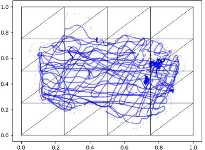
Figure 1: Data from a bathymetric survey in a triangular FEM grid. Data points are represented as blue dots.

Linear basis functions on their own are not enough to match the smoothing properties of the TPS. Consequently, a mixed finite element formulation was developed. As part of the formulation, Roberts et al. introduced auxiliary functions $\bm{u}$ to approximate the gradients of $s$, where

$$\bm{u}(\bm{x})=\begin{bmatrix}u_{1}(\bm{x})\\ \vdots\\ \ u_{d}(\bm{x})\end{bmatrix}=\begin{bmatrix}\bm{b}(\bm{x})^{T}\bm{g}_{1}\\ \vdots\\ \ \bm{b}(\bm{x})^{T}\bm{g}_{d}\end{bmatrix}.$$

Vectors $u_{k}(\bm{x})$ approximates the gradient of $s$ in dimension $k$ for $1\leq k\leq d$ and $\bm{g}_{1},\ldots,\bm{g}_{d}$ are the corresponding coefficients.

Given a data set $\left\{(\bm{x}_{i},y_{i}):i=1,2,\ldots,n\right\}$ of size $n$ and dimension $d$ on a bounded domain $\Omega$, where $\bm{x}_{i}\in\mathbb{R}^{d}$ and $y_{i}\in\mathbb{R}$ are $i$-th predictor value and response value, respectively, we find $s$ by minimising

$$J(\bm{c},\bm{g}_{1},\ldots,\bm{g}_{d}) =\frac{1}{n}\sum^{n}_{i=1}\left(\bm{b}(\bm{x}_{i})^{T}\bm{c}-y_{i}\right)^{2}+\alpha\int_{\Omega}\sum_{k=1}^{d}\nabla\left(\bm{b}\left(\bm{x}\right)^{T}\bm{g}_{k}\right)\nabla\left(\bm{b}\left(\bm{x}\right)^{T}\bm{g}_{k}\right)\,d\bm{x}$$

$$=\bm{c}^{T}A\bm{c}-2\bm{d}^{T}\bm{c}+\bm{y}^{T}\bm{y}/n+\alpha\sum_{k=1}^{d}\bm{g_{k}}^{T}L\bm{g_{k}},$$ (1)

subject to the constraint $L\bm{c}=\sum_{k=1}^{d}G_{k}\bm{g}_{k}$, where $\bm{y}=[y_{1},\ldots,y_{n}]^{T}$, $\bm{d}=\frac{1}{n}\sum_{i=1}^{n}\bm{b}(\bm{x}_{i})y_{i}$ and $A=\frac{1}{n}\sum_{i=1}^{n}\bm{b}(\bm{x}_{i})\bm{b}(\bm{x}_{i})^{T}$. Matrix $L$ is a discrete approximation to the negative Laplacian and $L_{p,q}=\int_{\Omega}\nabla\bm{b}_{p}\nabla\bm{b}_{q}\,d\bm{x}$. Matrix $G_{k}$ is a discrete approximation to the gradient operator in dimension $k$ for $1\leq k\leq d$ and $(G_{k})_{pq}=\int_{\Omega}\bm{b}_{p}\partial_{k}\bm{b}_{q}\,d\bm{x}$. The matrix $A$ and vector $\bm{d}$ are constructed by scanning the observed data, where $A=BB^{T}$ and $B_{p,i}=b_{p}(\bm{x}_{i})/\sqrt{n}$. Intuitively, the role of matrix $B$ is to project the data down onto the FEM grid. This is done by averaging the data that falls within the radius of support of a given basis function. Note that the $p$-th row of $B$ will be zero if none of the data points falls within the radius of support of $b_{p}$. Matrices $L$, $G_{k}$ and $A$ are $m\times m$ sparse matrices, where $m$ is the number of basis functions. This mixed finite element formulation is efficient for large data sets where $n>>m$.

The smoothing parameter $\alpha$ balances goodness of fit and smoothness of $s$, and may be calculated automatically using techniques such as the generalised cross-validation (GCV) discussed in Section 3.2.

By using Lagrange multipliers, Equation (2.1) and the given constraint can be rewritten as a system of linear equations [2]. For example, in a two-dimensional domain with Dirichlet boundary condition, the system is

$$\begin{bmatrix}A&\bm{0}&\bm{0}&L\\ \bm{0}&\alpha L&\bm{0}&-G_{1}^{T}\\ \bm{0}&\bm{0}&\alpha L&-G_{2}^{T}\\ L&-G_{1}&-G_{2}&\bm{0}\end{bmatrix}\begin{bmatrix}\bm{c}\\ \bm{g}_{1}\\ \bm{g}_{2}\\ \bm{w}\end{bmatrix}=\begin{bmatrix}\bm{d}\\ \bm{0}\\ \bm{0}\\ \bm{0}\end{bmatrix}-\begin{bmatrix}\bm{h}_{1}\\ \bm{h}_{2}\\ \bm{h}_{3}\\ \bm{h}_{4}\end{bmatrix},$$ (2)

where $\bm{w}$ is a Lagrange multiplier and Dirichlet boundary information is stored in $\bm{h}_{1}$, $\bm{h}_{2}$, $\bm{h}_{3}$ and $\bm{h}_{4}$. The $\bm{h}_{1},\cdots,\bm{h}_{4}$ vectors are not required in the case of Neumann boundary conditions. The original theory formulated by Roberts et al. used zero Neumann boundary conditions. We included both Dirichlet and Neumann boundary conditions in the numerical experiments as the Dirichlet boundary conditions allow us to set up and analyse problems with known solutions. Furthermore, the resulting system of equations with Dirichlet boundaries is better conditioned. In the examples presented in this paper, a sparse direct solver was used to solve the above saddle point problem. However, Stals [13] has studied the use of a preconditioned conjugate gradient method.

When using Dirichlet boundary conditions, the $\bm{g}_{k}$ vectors give an approximation to the gradient of the data. When using Neumann boundary conditions, the  $L$ and $G_{k}$ matrices have non-trivial null spaces and consequently $\bm{g}_{k}$ gives an approximation to the gradient of the data up to a constant.

Roberts et al. presented a convergence analysis for the TPSFEM with uniformly distributed data perturbed by white noise. They showed that the error convergence of the TPSFEM $s$ depends on the smoothing parameter $\alpha$, mesh size $h$ and the maximum distance between data points $d_{X}$ of its FEM grid. The mesh size $h=\max_{\tau\in\mathcal{T}^{h}}\text{diameter}(\tau)$ of a two-dimensional triangular FEM grid is defined as the longest edge of all triangles and the distance $d_{X}=\sup_{\bm{x}\in\Omega}\text{distance}\left(\bm{x},\{\bm{x}_{i}\}\right)$ be the maximum distance of any point in $\Omega$ from a data point. Suppose that the finite element spaces satisfy Assumptions 1 to 5 of [2], then there exist constants $C_{1}>1$ and $\alpha_{0}>0$ such that for all smooth function $f\in H^{2}(\Omega)$, which models response values $\bm{y}$, the expected errors of the TPSFEM satisfy

$$E||s(\bm{y})-f||_{L^{2}(\Omega)}^{2}\preceq\left(\alpha+h^{4}+d_{X}^{4}\right)||f||_{H^{2}(\Omega)}^{2}+\frac{\sigma^{2}}{\alpha^{1/2}}\frac{\left(h^{4}+d_{X}^{4}\right)}{h^{2}},$$ (3)

$$E|s(\bm{y})-f|_{H^{1}(\Omega)}^{2}\preceq\frac{1}{\alpha^{1/2}}\left(\alpha+h^{4}+d_{X}^{4}\right)||f||_{H^{2}(\Omega)}^{2}+\frac{\sigma^{2}}{\alpha}\frac{\left(h^{4}+d_{X}^{4}\right)}{h^{2}},$$ (4)

provided that $h$ and $\alpha$ satisfy $h>C_{1}d_{X}$ and $d_{X}^{4}+h^{4}<\alpha<\alpha_{0}$. The $L^{2}(\Omega)$ norm and Sobolev semi-inner-products $H^{1}(\Omega)$ and $H^{2}(\Omega)$ are defined in Section 2.1 of [2] and $\sigma^{2}$ is the variance of measurement errors.

Observe that when $\alpha$ or $d_{X}$ is large, the difference between the FEM approximation $s$ and the observed data $f$ may not necessarily be reduced by decreasing $h$ [14]. Since the distribution of data points is predetermined, $d_{X}$ cannot be modified. As opposed to PDE-based error indicators that focus solely on $h$, we must estimate an optimal $\alpha$ and $h$ to minimise the expected regression errors.

Roberts et al. assume the data points are uniformly spread in the sense that there exists a constant $C>1$ such that $d<C\min_{i\neq j}\left|\bm{x}_{i}-\bm{x}_{j}\right|$. See Assumption 5 of  [2]. We ensured this assumption held in our original study of a set of model problems used to validate the performance of the TPSFEM and our code. For the real-world problems shown in this article, the assumption no longer holds. Nevertheless, the behaviour of the numerical results is similar to what was observed previously with our model problems.

2.2 Comparison with radial basis functions

To validate the TPSFEM’s competitiveness, we compared the performance of the TPSFEM to the TPS [15] and several radial basis functions (RBFs) with compact support from Wendland [16] and Buhmann [17] using the Crater Lake survey [18] described in Section 5.

To find the control points for the RBFs, we place a rectangular grid over the domain and then randomly chose a point from each rectangle that contains any data. This idea is similar to what is shown in Figure 1, except rectangles are used instead of triangles. With this approach, it is possible to bound the maximum distance between neighbouring control points. Given the error estimate depends on the maximum distance between neighbouring points, we can construct a corresponding bound on the error estimate of the RBF that will decrease as the number of rectangles, and in turn the number of control points, is increased. Let $\bar{n}$ be the number of control points extracted from the Crate Lake data set.

Consider a control point $\bar{\bm{x}}_{i}$ where $1\leq i\leq\bar{n}$. The RBF kernel defined at point $\bar{\bm{x}}_{i}$ is $\Psi_{i}(\bm{x})=\Phi_{i}(r)$ where $r=||\bar{\bm{x}}_{i}-\bm{x}||_{2}$ is the Euclidean distance between $\bar{\bm{x}}_{i}$ and $\bm{x}$. Examples of $\Phi_{i}$ used in the paper are listed in Table 1. The function $(1-r)_{+}$ is a truncated power function and $(1-r)_{+}=0$ if $(1-r)<0$. Thus, the Wendland RBFs have compact support. The Buhmann’s RBFs also have compact support as the kernel is defined by $\Phi_{i}(r)=0$ if $r>1$. The three RBFs with compact support are scaled using a radius of support $\rho$ and the kernel values are calculated using $\Phi_{i}(r/\rho)$. An example heuristic approach to choosing $\rho$ is to aim to have a given, fixed, number of data points fall within the circle with centre $\bar{\bm{x}}_{i}$ and radius $\rho$. See [19]. In this report, the radius $\rho$ is calculated so that the local support of each kernel contains about 200 sampled data points. For instance, the radius of support when the number of sample points is 975, 3867 and 9010 are 0.15, 0.077 and 0.050, respectively.

The resulting RBF is $s_{rbf}(\bm{x})=\sum_{i=1}^{\bar{n}}w_{i}\Psi_{i}(\bm{x})$ for coefficients $w_{i}\in\mathbb{R}$. The TPSFEM is constructed using Dirichlet boundaries with uniform grids. The Dirichlet boundary conditions $\bm{h}_{i}$ are defined using constants described in Section 5.

The smoothing parameter $\alpha$ is calculated using the GCV as discussed in Section 3.2.

We compared the accuracy and efficiency of the different kernels using the five attributes listed in Table 1. The number of basis is $\bar{n}$ for the RBFs and $m$ for the TPSFEM. The accuracy of the approximation associated with each kernel is measured using the $\text{RMSE}=\big{(}\frac{1}{n}\sum_{i=1}^{n}\big{(}\hat{y}_{i}-y_{i}\big{)}^{2}\big{)}^{\frac{1}{2}}$, where $\hat{y}_{i}=s_{rbf}(\bm{x}_{i})$ for the RBF kernels and $\hat{y}_{i}=s(\bm{x}_{i})$ for the TPSFEM. We also evaluated their efficiency using the number and ratio of nonzero entries in the system of equations and the time to solve the system. The number and ratio of nonzero entries is a measure of the sparsity of the system, which may be exploited by sparse solvers [21]. Since sparse solvers may be affected by other factors like the structure of the systems, we also included the time for solving the system of equations, measured in seconds.

The program was implemented using Python 3.8, and we used a direct solver for the TPS and a sparse solver (PyPardiso) for both the TPSFEM and RBFs with compact.

Table 1: Comparison of computational costs

Technique	Kernel $\Phi_{i}$	# basis	# nonzero	Ratio	Time	RMSE
TPSFEM		4,225	181,352	7.2%	0.09	9.29
		16,641	608,642	1.5%	0.43	5.50
		33,025	1,306,933	0.8%	0.88	4.34
TPS	$r^{2}\log(r)$	975	950,625	100%	0.11	10.58
		3,867	14,953,689	100%	0.73	5.05
		9,010	81,180,100	100%	4.49	3.57
Wendland	$(1-r)^{2}_{+}$	975	77,677	8.2%	0.14	13.61
		3,867	373,575	2.5%	0.18	6.38
		9,010	955,734	1.18%	0.79	5.33
Wendland	$(1-r)^{4}_{+}(4r+1)$	975	77,671	8.17%	0.13	11.81
		3,867	373,469	2.5%	0.18	5.50
		9,010	955,700	1.18%	0.79	4.09
Buhmann	$1/3-4r^{3}/3$	975	77,677	8.17%	0.13	11.97
	$+2r^{2}\log(r)$	3,867	373,497	2.5%	0.17	5.65
		9,010	955,734	1.18%	0.69	4.51

As shown in Table 1, the RBFs with compact support achieved similar RMSE compared to the TPS, but required less time to solve the system of equations. The matrix associated with the TPS is a full matrix and therefore computationally expensive. The TPSFEM also has similar RMSE compared to the other smoothers and slightly higher system solving time despite the lower number of nonzero entries in the corresponding system.

We are aware the performance of the RBFs may be improved by adopting additional modifications such as a localised radius of support or more efficient parallel solvers [19]. Nevertheless, we believe this example demonstrates the TPSFEM’s competitiveness. While the experiment only concentrated on a single data set, a comprehensive comparison is in progress and will be provided in Stals [22]. In that paper, Stals also takes into account the time to construct the system of equations and evaluate the resulting basis function, for example. These experiments suggest that the RBFs work well in small to medium problems due to their higher accuracy. However, the TPSFEM scales much better in larger problems due to its more efficient structure. As demonstrated in Table 1, the system associated with the TPSFEM has fewer non-zeros compared to system associated with the RBFs, and that is beneficial for large data sets.

3 Adaptive refinement

Adaptive refinement is a process that iteratively refines elements in sensitive regions, such as peaks, to improve the accuracy of a solution [4]. Consequently, compared to uniform grids, adaptive grids require fewer nodes to reach a satisfactory solution. An error indicator is critical to adaptive refinement as it identifies these sensitive regions.

In this article, we examine adaptive refinement and error indicators over two-dimensional grids with triangular elements. The triangles are refined using the newest node bisection method. Each triangle will have one, and only one, vertex labelled as the newest node. A triangle is divided into two children triangles by adding an edge from the newest node to the middle point of the opposite edge [23]. That midpoint becomes the newest node for the next refinement iteration. This helps to prevent long thin triangles and limits the growth of the interpolation error [24].

In terms of the data structure we use to store the FEM grid, it is easier to work with the edges rather than the nodes. Given a triangle, the edge that sits opposite the newest nodes is labelled as a base-edge. Any two triangles that share a base-edge are called a triangle pair. During uniform refinement, all the triangles are bisected along the base-edge. The remaining old edges in each triangle become the new set of base-edges. This controls the order of refinement to, again, avoid long thin triangles. During adaptive refinement, only some of the triangle pairs are bisected. This may result in edges that are shared by coarse (old) and fine (new) triangles. Such edges are labelled as interface base-edges. Triangles can only be bisected along base-edges. If an interface base-edge is to be bisected, the coarse triangle sharing that edge is bisected first. That interface base-edge is then marked as a base-edge, and bisection can proceed for the triangle pair. This avoids hanging nodes. It is possible the neighbouring coarse triangle mentioned previously also contains an interface base-edge. A recursive algorithm is used to move down the neighbouring coarse triangles until a base-edge is found. Mitchell [3] and Stals [25] showed this recursive algorithm will terminate. These error indicators and the newest node bisection may also be extended to other dimensions [4]. We show more details of our iterative adaptive refinement process in Section 3.1 and how the smoothing parameter $\alpha$ is updated iteratively in this process in Section 3.2.

3.1 Iterative adaptive refinement process

The PDE-based iterative adaptive refinement process starts with a coarse initial grid and refines it iteratively using an error indicator until the solution reaches a given error tolerance [26]. In each iteration, elements with an error indicator value higher than a given error tolerance are marked and refined. A new solution is built using the refined grid and the error indicator values will be compared to the error tolerance to determine whether the iterative process should continue or terminate.

Error indicators developed for PDE formulations are generally based on the discretisation error of the FEM approximation. Consequently, their calculations are purely based on $h$. However, in our TPSFEM formulation, the approximation error is based on several factors, including $\alpha$, $h$ and $d_{X}$, as mentioned in Section 2.1. Therefore, standard PDE-based approaches may not work, especially in the case with large $\alpha$ or $d_{X}$ as demonstrated in Section 4 of [14].

Some PDE-based error indicators measure the rate of change and a smooth approximation will give small error indicator values, thus terminating the iterative process. However, this approach in TPSFEM may lead to premature termination. A smooth function does not necessarily fit the data and consequently the RMSE may still be high [27]. Therefore, the standard procedure described in Mitchell [3] does not work for the TPSFEM. A modified iterative process for the TPSFEM is shown in Algorithm 1 and it contains an additional inner loop at step 9. We iteratively mark and refine a small subset of elements with relatively high error indicator values in each iteration of the inner loop. This inner loop is guaranteed to add new nodes, and it terminates as soon as the FEM grid contains a preset number of nodes. In our experiments, we terminated the inner loop when the number of nodes has been doubled. The reason is that we intend to explore the use of the multigrid method as an iterative solver in future studies. However, this is a somewhat arbitrary choice and specific problems may benefit from a different choice. This inner loop avoids the limitations of a pre-set error tolerance for large $\alpha$ and $d_{X}$.

Referring to Algorithm 1, when elements are refined, new nodes added in triangular grid $\mathcal{T}_{k,j+1}$ take average values of their neighbouring nodes. We do not solve Equation (2) until the inner loop terminates. We use $s_{k}$ and $s_{k,j+1}$ to represent the smoother $s$ defined on grid $\mathcal{T}_{k}$ and $s$ that is defined on grid $\mathcal{T}_{k,j+1}$. Since new nodes take average values of neighbouring nodes, $s_{k,j+1}$ is only an approximation. We work with the approximation because solving Equation (2) each time a new node is added would be exorbitantly expensive. However, only using an approximation may affect the performance of the error indicators. This is a trade-off between cost and accuracy. After this procedure terminates, the full system is solved to improve the accuracy of $s$. This allows us to estimate the RMSE of updated $s$ stored in $s_{k+1}$ for the stopping criteria.

Algorithm 1 Solve TPSFEM with adaptive refinement

1:$k\leftarrow 0$

2:calculate optimal $\alpha_{k}$ on initial coarse grid $\mathcal{T}_{k}$

3:solve Equation (2) for TPSFEM $s_{k}$ on $\mathcal{T}_{k}$

4:evaluate RMSE of $s_{k}$

5:while RMSE is higher than error tolerance do

6:     calculate error indicators for edges in $\mathcal{T}_{k}$

7:     $j\leftarrow 0$

8:     $\mathcal{T}_{k,j}\leftarrow\mathcal{T}_{k}$

9:     while size of $\mathcal{T}_{k,j}$ is smaller than twice of size of $\mathcal{T}_{k}$ do

10:         mark a subset of elements with high error indicator values

11:         refine marked elements to construct $\mathcal{T}_{k,j+1}$ and obtain $s_{k,j+1}$ by averaging

12:         calculate error indicators for new edges in $\mathcal{T}_{k,j+1}$

13:         $j\leftarrow j+1$

14:     end while

15:     $\mathcal{T}_{k+1}\leftarrow\mathcal{T}_{k,j}$

16:     calculate optimal $\alpha_{k}$ on refined grid $\mathcal{T}_{k+1}$

17:     solve Equation (2) for TPSFEM $s_{k+1}$ on $\mathcal{T}_{k+1}$

18:     evaluate RMSE of $s_{k+1}$

19:     if RMSE is reduced less than 10% for two iterations then

20:         break

21:     end if

22:     $k\leftarrow k+1$

23:end while

Traditional stopping criteria of the iterative process are based on fixed error tolerance for errors approximated by error indicators [4]. In contrast, our new stopping criteria are a combination of fixed error tolerance and rates of change of the RMSE [28]. The iterative process stops when the RMSE of $s$ is lower than the error tolerance. Note the RMSE may not converge to zero if the data is not smooth enough or perturbed by noise [27]. We terminate the iterative process when the addition of new nodes ceases to significantly reduce the RMSE. Specifically, we terminate the iterative process when the RMSE is reduced less than 10% by one iteration of refinement for two consecutive iterations. This criterion performed well in previous experiments given various model problems, data sizes and noise levels shown in Chapter 8 of [27].

3.2 Smoothing parameter

The generalised cross-validation (GCV) is a popular statistical technique for model validation and variable selection. Golub [29] developed the GCV method to estimate the ridge parameter for use in ridge regression. The GCV must calculate the trace of a matrix inverse to estimate $\alpha$, which is expensive for medium to large-scale problems. Hutchinson [30] approximated the trace term using an unbiased stochastic estimator that was used by Roberts et al. [2] and Stals and Roberts [12].

The error convergence rates of $s$ depend on the smoothing parameter $\alpha$ as discussed in Section 2.1. The value of an optimal $\alpha$ is affected by a range of factors, including the size, noise level and smoothness of the observed data; and $h$. Stals and Roberts [13] investigated a wide range of $\alpha$ values from $10^{-10}$ to $1$ to test the robustness of solvers. In practice, the optimal $\alpha$ of the TPSFEM often ranges from $10^{-10}$ to $10^{-4}$.

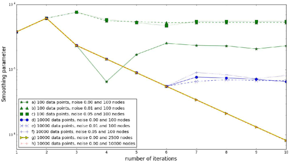
Figure 2: $\alpha$ values at each iteration of bounded minimisation with various numbers of data, nodes and noise levels.

The iterative process in Algorithm 1 calculates a new $\alpha$ in each iteration. Note that the value of $\alpha$ found in iteration $k$ is labelled as $\alpha_{k}$. We speed up the computation of $\alpha_{k}$ in iteration $k$ using $\alpha_{k-1}$ from the previous iteration [31]. Fang [27] argued the optimal $\alpha$ generally decreases as $h$ decreases with each refinement iteration until stabilising inside a fixed range. An example from Fang is shown in Figure 2, where $\alpha$ values were obtained for different $h$ using the Brent method [32]. Therefore, $\alpha_{k}$ is calculated as $\alpha_{k}=\arg\min\{V(\alpha_{k-1}),V(r_{1}\alpha_{k-1}),V(r_{2}\alpha_{k-1})\}$ where $0<r_{1},\,r_{2}<1$. Function $V(\alpha)$ is the GCV function evaluated at $\alpha$ using Hutchinson’s method to approximate the trace. In our experiments, we chose $r_{1}=0.1$ and $r_{2}=0.3$, which are consistent with the convergence of $\alpha$. The $\alpha_{0}$ value for the initial grid in Algorithm 1 is still computed using bounded minimisation within interval $[10^{-10},~{}10^{-4}]$. This approach is simple but robust, especially given that small changes in $\alpha$ do not have a marked impact on $s$. Fang showed this approach produces results similar to Brent’s method [32] which required ten evaluations of $V$. The experiments were carried out on both uniform and adaptive refinement for various data sets and noise levels.

4 Error indicators

Given our focus is on data regression, we first explore the use of regression metrics as an error indicator in Section 4.1. As an alternative approach, four PDE-based error indicators were adapted for the TPSFEM. Namely, the auxiliary problem error indicator, residual-based error indicator, recovery-based error indicator and norm-based error indicator. More details are given in Chapter 5 of [27]. Two of the error indicators use global information like the grid and smoother $s$, and the other two also use local data points directly. A brief description of the four PDE-based error indicators is given in Sections 4.2 to 4.5.

The error indicator values are assigned to the base and interface base edges introduced in Section 3. In the approaches described below, the calculations are performed on all triangles sharing the specified edge. In the interior of the domain this will be a pair of triangles, along the boundary it may be a single triangle.

4.1 Regression metric as an error indicator

Since the observed data is available for the TPSFEM, we explored several approaches that use data directly to indicate errors, including regression metrics [5]. While many regression metrics like the RMSE were developed to assess surface fitting techniques, they have not been used for adaptive refinement.

The RMSE is measured locally by computing the difference between smoother $s$ and the data points lying inside a triangle. Specifically, consider an edge $e$. Let $\tau_{e}$ be the set of triangles that have $e$ as an edge. Furthermore, let $\{(\hat{\bm{x}}_{i},\hat{y}_{i}):i=1,2,\ldots,n_{e}\}$ be the set of data points lying inside $\tau_{e}$. If a data point sits on a vertex or an edge, it is only included in the calculation for one triangle. Thus, it is not counted multiple times. The error indicator value $\eta_{e}$ is calculated as

$$\boxed{\eta_{e}=\left(\frac{1}{n_{e}}\sum_{i=1}^{n_{e}}\left(s\left(\hat{\bm{x}}_{i}\right)-\hat{y}_{i}\right)^{2}\right)^{\frac{1}{2}}.}$$

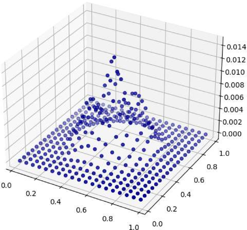
(a)

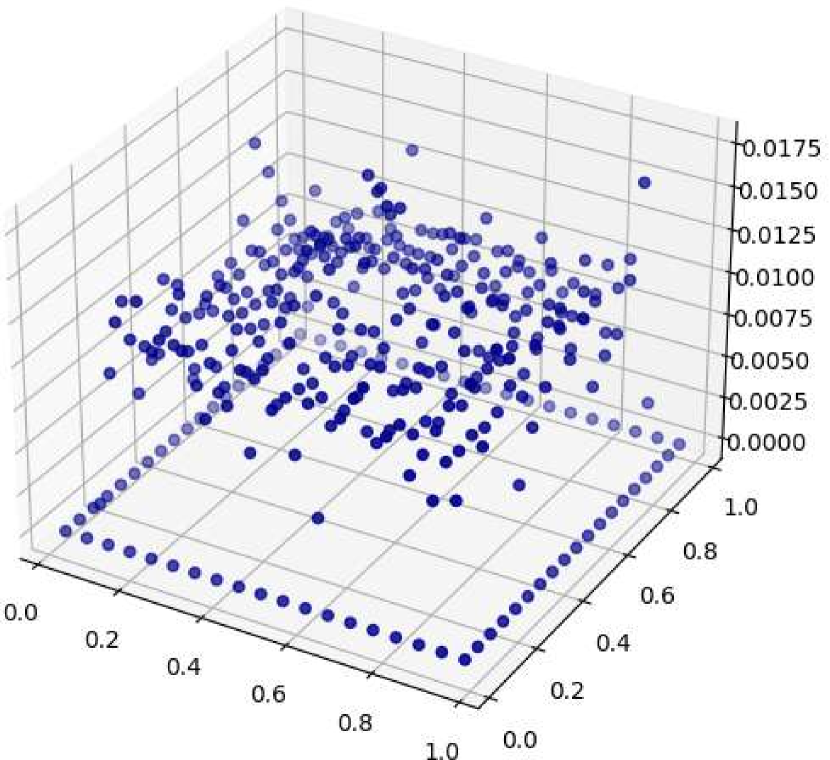
(b)

Figure 3: RMSE of $s$ against data sets modelled by $y=e^{-50(x_{1}-0.5)^{2}}e^{-50(x_{2}-0.5)^{2}}$ (a) without noise; and (b) with Gaussian noise. The points represent RMSE in each triangle pair.

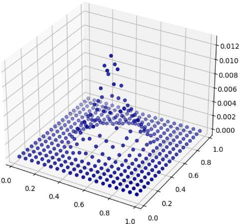
(a)

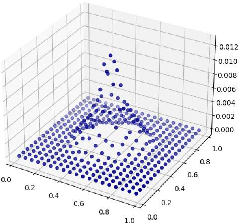
(b)

Figure 4: Recovery-based error indicator values for the data set modelled by $y=e^{-50(x_{1}-0.5)^{2}}e^{-50(x_{2}-0.5)^{2}}$ (a) without noise; and (b) with Gaussian noise. The points represent error indicator values in each triangle pair.

We tested the RMSE as an error indicator using a two-dimensional uniformly distributed data set of size $1\times 10^{4}$ in $[0,1]^{2}$ square domain using a uniform FEM grid with 400 nodes. The tests were carried out without noise and in the presence of Gaussian noise with mean zero and standard deviation 0.01. The range of $\hat{y}$ values is 0 to 1. The resulting error indicator values are shown in Figure 3. When the data is not perturbed by noise, the RMSE is high at the centre as shown in Figure 3(a). The model problem changes more rapidly in this region and indicated high RMSE suggests more refinement is required at the centre. However, the RMSE no longer provides useful information when the data is perturbed by noise as shown in Figure 3(b) and is thus not an effective error indicator in that scenario. Furthermore, the RMSE does not work if there are elements without data points, which has consequences for applications like surface reconstructions [6]. Several other regression metrics were tested, and they performed poorly in the presence of noise. Moreover, they are sensitive to changes in data distribution patterns and may lead to over-refinement.

For comparison, we reran the experiment using the PDE-based error indicator defined in Section 4.4. The results are provided in Figure 4. The recovery-based error indicator accesses the data indirectly and is less sensitive to noise. Its error indicator values in Figures 4(a) and 4(b) are almost identical. We tested the regression as an error indicator and provided more statistics and adaptive grids in Section 5.1.

4.2 Auxiliary problem error indicator

The auxiliary problem error indicator solves an auxiliary problem on smaller domains to obtain locally more accurate approximations [33, 34]. The error of the solution is approximated locally by the difference between the global approximation $s$ and a local approximation with improved accuracy. Similar ideas have also been applied in surface fitting techniques to assess approximation quality using a cluster of neighbouring data points [35].

As in Section 4.1, let $e$ be a base or interface base edge, and $\tau_{e}$ be the set of triangles sharing that edge. We then define a local grid $\mathcal{T}_{e}$ to be all the triangles that share a node with the triangles in $\tau_{e}$. For example, referring to Figure 5, $e$ is the edge between nodes $N_{1}$ and $N_{2}$, $\tau_{e}$ contains the triangles $\{N_{1},N_{2},N_{3}\}$ and $\{N_{1},N_{2},N_{4}\}$, and the local grid is all the triangles that share the nodes $N_{1}$, $N_{2}$, $N_{3}$ and $N_{4}$. Finally, let $\Omega_{e}$ be the local domain whose boundary coincides with the boundary of $\mathcal{T}_{e}$. We take $\Omega_{e}$ to have Dirichlet boundary conditions.

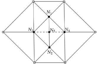
Figure 5: An example local domain. Interior nodes and boundary nodes are represented as filled circles and open circles, respectively. Accuracy is improved by refining edge $N_{1}\text{-}N_{2}$ to introduce a new vertex $N_{5}$ and new edges represented as dashed lines.

To define the improved local approximation, we bisect the triangles along the edge $e$ to obtain the grid $\hat{\mathcal{T}}$. We treat interface-base and base edges the same as this is a temporary change to the grid. The grid in Figure 5, with node $N_{5}$, is an example of $\hat{\mathcal{T}}$. Let  $\{(\hat{\bm{x}}_{i},\hat{y}_{i}):i=1,2,\ldots,n_{e}\}$ be the subset of the observed data that sits inside $\Omega_{e}$. The local approximation $\hat{s}=\hat{\bm{b}}(\bm{x})^{T}\hat{\bm{c}}$ is built by minimising the functional

$$J_{\alpha}\left(\hat{\bm{c}},\hat{\bm{g}}_{1},\ldots,\hat{\bm{g}}_{d}\right)=\frac{1}{{n_{e}}}\sum^{{n_{e}}}_{i=1}\left(\hat{\bm{b}}(\hat{\bm{x}}_{i})^{T}\hat{\bm{c}}-\hat{y}_{i}\right)^{2}+\alpha\int_{{\Omega_{e}}}\sum_{k=1}^{d}\nabla\left(\hat{\bm{b}}(\hat{\bm{x}})^{T}\hat{\bm{g}}_{k}\right)\nabla\left(\hat{\bm{b}}(\hat{\bm{x}})^{T}\hat{\bm{g}}_{k}\right)\,d\bm{x}$$ (5)

subject to constraint $\hat{L}\hat{\bm{c}}=\sum_{k=1}^{d}\hat{G}_{k}\hat{\bm{g}}_{k}$. Dirichlet boundary conditions applied to the local domain ${\Omega_{e}}$ are taken from the current global solution $s$. So, if node $p$ sits on the boundary of $\Omega_{e}$,

$$\hat{c}_{p}=c_{p},\quad\hat{g}_{1,p}=g_{1,p},\quad\hat{g}_{2,p}=g_{2,p},\,\quad\cdots\quad\hat{g}_{d,p}=g_{d,p},\,\quad\hat{w}_{p}=w_{p}$$

where ${g}_{k,p}$ is the $p$-th entry of $\bm{g}_{k}$.

The error indicator value $\eta_{e}$ of triangular elements $\tau_{e}$ is based on the energy norm as suggested by Babuvška and Rheinboldt [34], where

$$\boxed{\eta_{e}^{2}=\int_{\tau_{e}}\left[\sum_{k=1}^{2}\left(\frac{\partial}{\partial x_{k}}\left(s-\hat{s}\right)\right)^{2}\right]\,d\bm{x}.}$$

Recall from Equation (3), the expected error of the TPSFEM is written in terms of $\alpha+h^{4}+d_{X}^{4}$. Consider the data distribution illustrated by data points in an example domain with triangles $\tau_{1}$, $\tau_{2}$, $\tau_{3}$ and $\tau_{4}$ in Figure 6. We can calculate local values for $d_{X}$ using the data given in triangles $\tau_{1}$, $\tau_{2}$ or $\tau_{3}$ directly using the definition given in Section 2.1. However, the subdomain in $\tau_{4}$ only has one data point and $d_{X}$ is no longer locally defined. Consequently, the solution $s$ in $\tau_{4}$, defined on $\Omega$, can be very different to the solution $\hat{s}$ in $\tau_{4}$, defined on ${\Omega_{e}}$. Furthermore, the second term $\frac{\sigma^{2}}{\alpha^{1/2}}\frac{(h^{4}+d_{X}^{4})}{h^{2}}$ of equation (3) shows the effects of the noise may be more prominent in subdomains with few data points and thus, potentially, larger values of $d_{X}$. More specifically, due to the potential difference in data distribution patterns, the behaviour of the solution in a local domain may vary dramatically compared to that in a global domain. In examples where the data is distributed evenly across the whole domain, such as image processing, the auxiliary problem error indicator is a viable option. However, if the data distribution is uneven, the behaviour of the solution can vary rapidly in the local subdomains. The consequences are readily seen in examples in Figure 17 from the numerical experiments in Section 5.2 below.

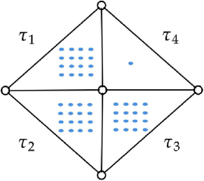
Figure 6: An example local domain with uneven data densities. Nodes and data points are represented as open circles and filled blue circles, respectively. The local domain contains four triangular elements, where elements $\tau_{1}$, $\tau_{2}$, $\tau_{3}$ have markedly more data points than $\tau_{4}$.

4.3 Residual-based error indicator

The residual-based error indicator estimates the energy norm of FEM approximation errors, which is represented as a combination of integrals of interior element residuals $r_{e}$ and jumps of gradients $j_{e}$ across the element boundaries [4]. The TPSFEM has a different formulation compared to PDEs and the residual cannot be calculated directly. Our alternative approach is to work with locally refined grids, similar to the one shown in Figure 5.

Let $e$ be a base or interface base edge, and $\tau_{e}$ be the set of triangles sharing that edge. Using the procedure described in Section 4.2, construct a grid $\mathcal{T}_{e}$ defined on a local domain ${\Omega}_{e}$. Finally, take $\hat{\mathcal{T}}$ to be the result of bisecting edge $e$ in $\mathcal{T}_{e}$.

Let $S\bm{p}=\bm{q}$ be the system defined in Equation (2) where $S$, $\bm{p}$ and $\bm{q}$ are the matrix, solution vector and right-hand side vector, respectively. And let $\hat{S}\hat{\bm{p}}=\hat{\bm{q}}$ be the corresponding system for the local grid $\hat{\mathcal{T}}$. Set $\mathbf{p}_{e}$ be the values of $\mathbf{p}$ restricted to grid $\mathcal{T}_{e}$. The residual $\bm{r}_{e}$ is then calculated as

$$\mathbf{r}_{e}=\hat{S}(I\bm{p}_{e})-\hat{\bm{q}}$$

where $I$ is a linear interpolation operator that maps from functions defined on $\mathcal{T}_{e}$ to functions defined on $\hat{\mathcal{T}}$. In terms of Figure 5, the values assigned to node $N_{5}$ is the average of the values assigned to nodes $N_{1}$ and $N_{2}$. When calculating the error indicator, only the first block of $\mathbf{r}_{e}$ that corresponds to the $\mathbf{c}$ coefficients is used. We use $\left.\mathbf{r}_{e}\right|_{c}$ to represent that block.

The jump $\mathbf{j}_{e}$ for the edge $e$ shared between triangle $\tau$ and triangle $\tau^{\prime}$ is

$$\mathbf{j}_{e}=\bm{n}\cdot\nabla s_{\tau}+\bm{n}^{\prime}\cdot\nabla s^{\prime}_{\tau},$$

where $s_{\tau}$ an $s^{\prime}_{\tau}$ are FEM approximations of $s$ on $\tau$ and $\tau^{\prime}$, respectively; and $\bm{n}$ and $\bm{n}^{\prime}$ are unit outward normal vectors to the edge $e$ in  $\tau$ and $\tau^{\prime}$, respectively. If $e$ lies on Dirichlet boundaries, $\mathbf{j}_{e}=0$. If $e$ lies on Neumann boundaries, $\mathbf{j}_{e}=-\bm{n}\cdot\nabla s_{\tau}$. The error indicator value $\eta_{e}$ of element $\tau_{e}$ is computed as

$$\boxed{\eta_{e}^{2}=c_{1}h_{e}^{2}\left\|\left.\mathbf{r}_{e}\right|_{c}\right\|_{L^{2}(\hat{\mathcal{T}})}^{2}+c_{2}h_{e}\left\|j_{e}\right\|_{L^{2}(\partial\tau_{e})}^{2},}$$

where $h_{e}$ is the mesh size of $\tau_{e}$, $c_{1}$ and $c_{2}$ are constants that balance the contributions from the residual and jump, respectively [4].

4.4 Recovery-based error indicator

The recovery-based error indicator calculates the error norm by post-processing discontinuous gradients of the TPSFEM smoother $s$ across inter-element boundaries [36]. The TPSFEM $s$ is represented by piecewise linear basis functions with zero-order continuity $C^{0}$ and the corresponding gradient approximation $D^{1}s$ are piecewise constants as illustrated in Figure 7. The gradient approximation $D^{1}s$ is post-processed to obtain an improved discrete gradient approximation $\hat{D}^{1}s$, which is closer to true gradients if the solution is smooth [4].

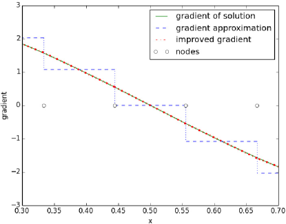
Figure 7: An one-dimensional example of improved gradients of FEM approximations.

The improved gradient $\hat{D}^{1}s$ is determined by the $L^{2}$-projection

$$\int_{\Omega}b_{p}\left(\hat{D}^{1}s-D^{1}s\right)\,d\mathbf{x}=0,\qquad p=1,\ldots,m.$$

This leads to a system of equations

$$\sum_{q=1}^{m}\int_{\Omega}b_{p}b_{q}\hat{D}^{1}s_{q}\,d\mathbf{x}=\int_{\Omega}b_{p}D^{1}s\,d\mathbf{x},\qquad p=1,\ldots,m,$$

where $\hat{D}^{1}s_{q}$ is the improved gradient $\hat{D}^{1}s$ evaluated at $q$-th node. The error is then estimated using the difference between current and improved gradients and the error indicator value $\eta_{e}$ of element $\tau_{e}$ is thus set as

$$\boxed{\eta_{\tau_{e}}^{2}=\int_{\tau_{e}}\left(\hat{D}^{1}s-D^{1}s\right)^{2}\,d\bm{x}.}$$

For PDEs, theoretical and experimental results show this error bound is asymptotically exact up to higher order terms, and it is shown to be effective for smooth functions $f\in H^{1}(\Omega)$ with surface load $g\in H^{1}(\partial\Omega_{N})$ on Neumann boundaries in Theorem 2.1 of [37]. The theory developed by Roberts et al. [2] assumes functions $f\in H^{2}(\Omega)$ with zero Neumann boundary conditions. Consequently, since the functions and boundary conditions for the TPSFEM are assumed to be smooth, we deduce this error indicator is worth considering for the TPSFEM.

The process above only uses $\bm{c}$ values to calculate improved gradient values $\hat{D}^{1}s$. We calculate both $\bm{c}$ and $\bm{g}$ values when solving Equation (2), and $\bm{g}$ values approximate the gradients of $s$. Suggesting we could use $\bm{u}$, defined in Section 2.1, when calculating the error indicator. Equations (3) and (4) show that the $L_{2}$ and $H_{1}$ norms of the TPSFEM are bounded by $\frac{\sigma^{2}}{\alpha^{1/2}}\frac{(h^{4}+d_{X}^{4})}{h^{2}}$ and $\frac{\sigma^{2}}{\alpha}\frac{(h^{4}+d_{X}^{4})}{h^{2}}$, respectively, when the variance $\sigma^{2}$ of noise is nonzero. Given that generally $\alpha\leq 1$, this suggests the gradient is more sensitive to noise. This is illustrated by a numerical experiment in Section 5.5 of [27]. Therefore, we chose to compute improved gradients using $\bm{c}$ values for the recovery-based error indicators.

4.5 Norm-based error indicator

The norm-based error indicator uses an error bound on the $L_{\infty}$ norm of the interpolation error [38]. Assuming the solution $f$ has bounded second-order derivatives, Sewell demonstrated the error of a two-dimensional FEM grid with first-order basis functions is bounded in terms of second-order derivatives $D^{2}_{\text{max}}f$, where

$$D^{2}_{\text{max}}f\left(x_{1},x_{2}\right)=\max_{i+j=2}\left|\partial^{2}f\left(x_{1},x_{2}\right)/\partial x_{1}^{i}x_{2}^{j}\right|.$$

He showed that a near-optimal grid with piecewise linear approximation will have $\int_{\tau_{i}}D^{2}_{\text{max}}f\,d\bm{x}$ equally distributed over all elements $\tau_{i}$. This error indicator identifies regions where the solution changes rapidly (high integral values) and resolves them using finer elements (smaller $h$) to achieve the required accuracy.

In contrast to the PDEs, the accuracy of the TPSFEM smoother $s$ is also affected by $\alpha$ and $d_{X}$ as shown in Equation (3). If either $\alpha$ or $d_{X}$ is large, the TPSFEM will interpolate a flat surface and this error indicator will refine evenly to distribute $\int_{\tau_{i}}D^{2}_{\text{max}}s\,d\bm{x}$ across the domain. If $\alpha$ and $d_{X}$ is sufficiently small, this error indicator will concentrate on reducing $h$ on regions with high expected errors to produce an efficient grid.

For two-dimensional grids, we approximate second-order derivatives with respect to $x_{1}$ and $x_{2}$ on each node and $D^{2}_{\text{max}}s$ is calculated as

$$D^{2}_{\text{max}}s\approx\max\left\{\left|D_{x_{1}x_{1}}s\right|,\left|D_{x_{1}x_{2}}s\right|,\left|D_{x_{2}x_{2}}s\right|\right\}.$$

The error indicator value assigned to edge $e$ is defined as

$$\boxed{\eta_{e}=\int_{\tau_{e}}D^{2}_{\text{max}}s\,d\bm{x},}$$

where $\tau_{e}$ is the set of triangles sharing the edge $e$. The error bound was derived under the assumption that the model problem has bounded second-order derivatives. Since the smoother $s$ of the TPSFEM in Equation (2.1) is minimised with respect to its second-order derivatives, the error bound naturally holds for the TPSFEM.

5 Numerical experiment

We evaluated adaptive refinement for the TPSFEM using three data sets: data generated using the peaks function from MATLAB, the 2000 Multibeam sonar survey of Crater Lake [18] and a bathymetric sounding survey of a coastal region [39]. The first data set consists of 62,500 data points uniformly distributed inside the $[-2.4,2.4]^{2}$ region of a $[-3,3]^{2}$ finite element domain and is modelled by

$$y=3\left(1-x_{1}\right)^{2}\exp\left(-\left(x_{1}^{2}\right)-\left(x_{2}+1\right)^{2}\right)-10\left(\frac{x_{1}}{5}-x_{1}^{3}-x_{2}^{5}\right)\exp\left(-x_{1}^{2}-x_{2}^{2}\right)-\frac{1}{3}\exp\left(-\left(x_{1}+1\right)^{2}-x_{2}^{2}\right)+\epsilon.$$ (6)

The peaks function has three local maxima and three local minima around the centre of the domain, and small flat surfaces near four corners. The data is perturbed by Gaussian noise $\epsilon$ with mean $0$ and standard deviation $0.02$. The performance of the TPSFEM on this model problem is discussed in Section 5.1. The Crater Lake survey comprises 12,936,068 data points consisting of latitude, longitude and elevations above sea level from a multibeam bathymetric survey of Crater Lake, Oregon in the United States. The survey collected over 16 million soundings and the data portrays the bottom of Crater Lake at a spatial resolution of 2 meters. The Crater Lake data is used to compare the performance of the TPSFEM with Dirichlet and Neumann boundaries in Section 5.2. The Coastal Region survey comprises 48,905 data points consisting of North American Datum of 1983 and modern readings of mean low water in meters. The mean low water is the average of all the low water heights observed over the National Tidal Datum Epoch. These measurements were taken to provide an estimate of historical bathymetry for the Mississippi-Alabama coastal region to aid geologic and coastal hazards studies. In Section 5.3, the Coastal Region data forms the basis of an investigation into the performance of the TPSFEM in a non-rectangular domain. The performance of uniform and adaptive grids is measured using the root-mean-square error (RMSE) versus the number of nodes, where $\text{RMSE}=\big{(}\frac{1}{n}\sum_{i=1}^{n}\left(s(\bm{x}_{i})-y_{i}\right)^{2}\big{)}^{\frac{1}{2}}$.

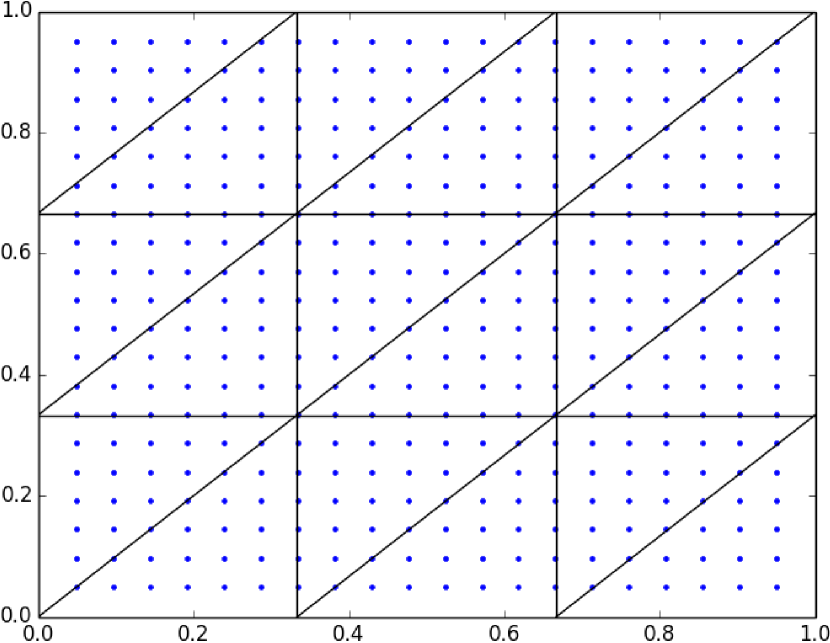
(a)

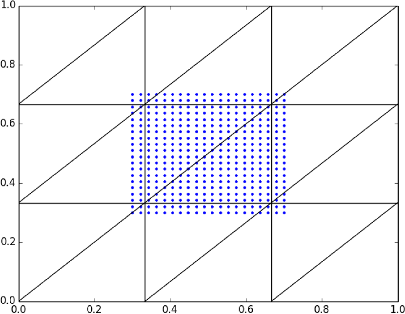
(b)

Figure 8: Example FEM grids with data points (a) close to boundaries; and (b) far away from boundaries. Data points are represented as blue points.

Dirichlet boundary conditions are set using the $\bm{h}_{1},\cdots,\bm{h}_{4}$ vectors in Equation (2). If the exact boundary conditions are known, the data can be placed near the boundaries of the domain as illustrated in Figure 8(a). In general, however, such an approach is not possible. The theoretical analysis given in [2] assumes zero Neumann boundary conditions. In other words, it assumes the solution is flat near the boundary, which is not necessarily the case. Consequently, if the boundary conditions are not known, the data points are placed well inside the domain as shown in Figure 8(b). In summary, when it is possible to approximate the boundary conditions, it is advantageous to use Dirichlet boundary conditions. Otherwise, the FEM grid is extended well past the boundary of the data set and Neumann boundary conditions are applied.

We observe in Figure 8(b) that the distribution of the data points can vary greatly from element to element. Some of the elements near the boundary only have 1 or 2 data points, whereas those in the interior have many data points. As discussed in Section 5, this may affect the accuracy of the local approximation of the auxiliary problem error indicator.

5.1 Results: peaks function

Two adaptive grids for the peaks function data in Equation (6) generated using norm-based error indicator and the regression metric are shown in Figures 9(a) and 9(b), respectively. The description of these two error indicators is given in sections 4.5 and 4.1. Refinement in the grid shown in Figure 9(a) is concentrated at the peaks in the centre of the domain. There is some refinement away from the centre of the domain. This is partly due to the use of interface base-edges to avoid hanging nodes as described in Section 3. It is also due to the fact that once the grid is fine enough in the centre, the error indicator will pick up some of the regions away from the centre of the domain. The norm-based error indicator has identified regions that change more rapidly. In contrast, the adaptive grid generated using the regression metric as an error indicator shown in Figures 9(b) contains over-refinement in many small regions. These results further confirm tha the regression metric is sensitive to noise as discussed in Section 4.1. Consequently, they are not considered for further testing.

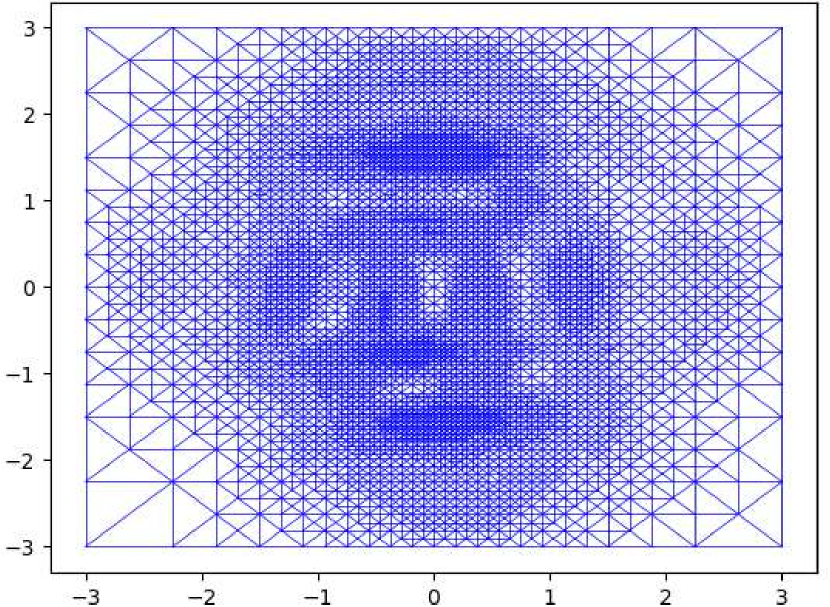
(a)

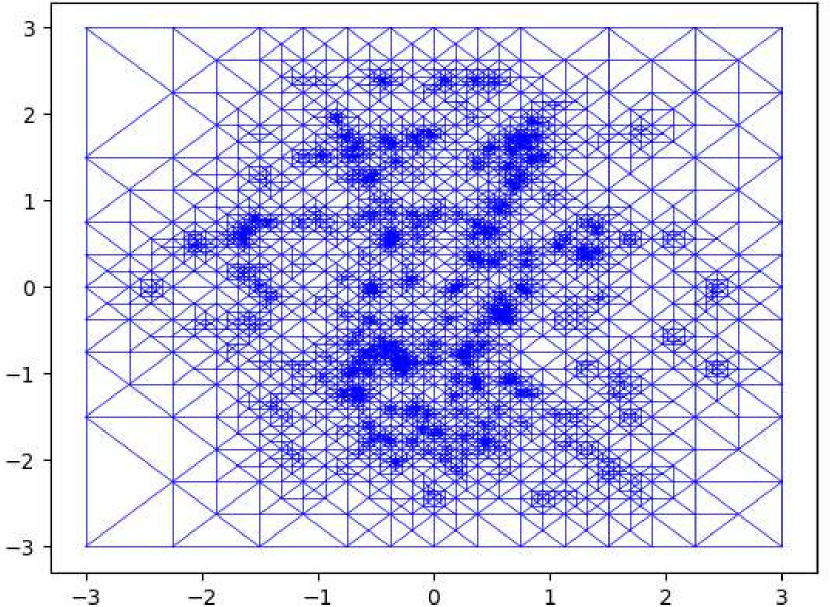
(b)

Figure 9: Adaptive grids using (a) norm-based error indicator; and (b) regression metric.

The convergence of the RMSE of the TPSFEM using uniform and adaptive grids for the peaks function data with Dirichlet and Neumann boundaries is shown in Figures 10(a) and 10(b), respectively. The initial square grids contain 25 nodes and are refined using uniform and adaptive refinement for at most 10 and 8 iterations, respectively. The adaptive grids produced by the four error indicators have similar error convergence rates for both Dirichlet and Neumann boundaries, which are significantly higher than that of the uniform grid. While the adaptive grids produced by the regression metric achieve similar error convergence for the first three iterations, the error convergence slows down, and the final grids have the highest RMSE.

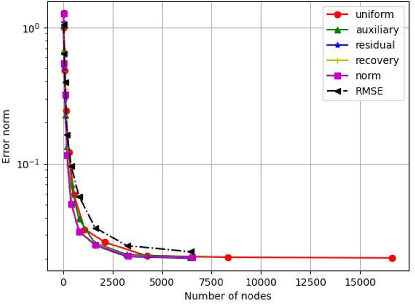
(a)

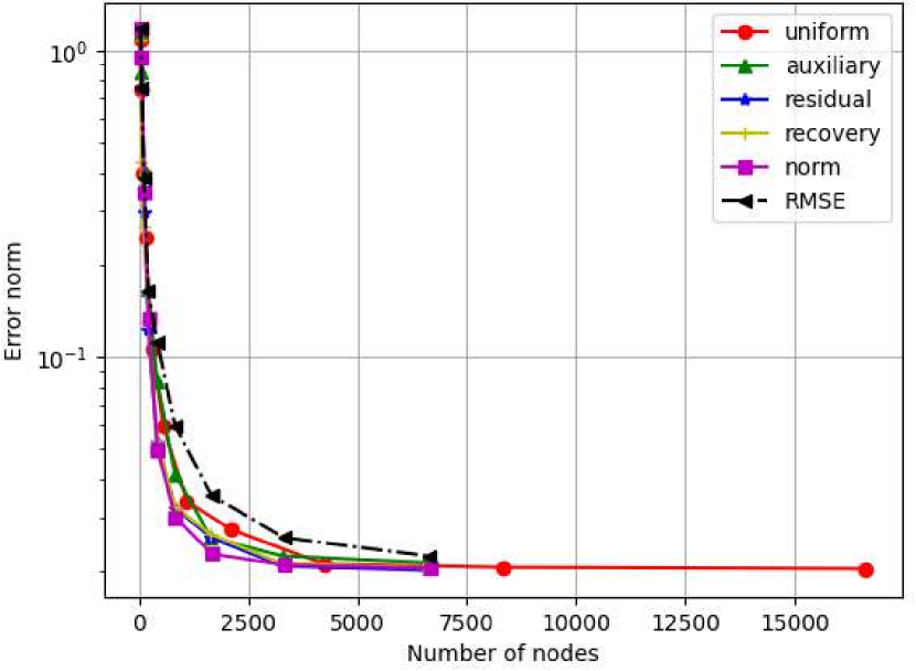
(b)

Figure 10: RMSE of TPSFEM using uniform and adaptive grids with (a) Dirichlet boundaries; and (b) Neumann boundaries.

We also list the RMSE, root-mean-square percentage errors (RMSPE), maximum residual errors (MAX), numbers of nodes of the final grids and the time to solve the system of equations in seconds in Table 2. The RMSPE is calculated as $\text{RMSPE}=\big{(}\frac{1}{n}\sum_{i=1}^{n}\left((s(\bm{x}_{i})-y_{i})/{y_{\max}}\right)^{2}\big{)}^{\frac{1}{2}}$, where $y_{\max}=\max(\bm{y})$. The adaptive grids using the four error indicators achieve similar RMSE, RMSPE and MAX using about $39.22\%$ of the number of nodes and about $46.39\%$ of the solve time compared to the uniform grids. While the adaptive grids produced by the regression metric have similar MAX to some other adaptive grids, their RMSE and RMSPE are significantly higher and are therefore less efficient.

Table 2: Regression metrics of the TPSFEM for peak function

Boundary	Metric	Uniform	Auxiliary	Residual	Recovery	Norm	Regression
Dirichlet	RMSE	0.021	0.021	0.021	0.021	0.021	0.023
	RMSPE	$2.50\times 10^{-3}$	$2.52\times 10^{-3}$	$2.47\times 10^{-3}$	$2.51\times 10^{-3}$	$2.51\times 10^{-3}$	$2.77\times 10^{-3}$
	MAX	0.093	0.093	0.11	0.094	0.093	0.11
	# nodes	16641	6404	6456	6561	6536	6468
	Time	0.41	0.21	0.21	0.20	0.19	0.21
Neumann	RMSE	0.021	0.022	0.020	0.021	0.021	0.022
	RMSPE	$2.51\times 10^{-3}$	$2.63\times 10^{-3}$	$2.48\times 10^{-3}$	$2.53\times 10^{-3}$	$2.51\times 10^{-3}$	$2.76\times 10^{-3}$
	MAX	0.095	0.10	0.10	0.11	0.10	0.11
	# nodes	16641	6538	6564	6496	6660	6627
	Time	0.49	0.22	0.22	0.22	0.20	0.22

5.2 Results: Crater lake

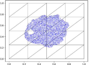
Figure 11: Randomly sampled data points in initial FEM grids for Crater Lake data. Data points are represented as blue dots.

We scaled and fitted the Crater Lake data inside the $[0.2,0.8]^{2}$ region and used $[0,1]^{2}$ as the finite element domain as illustrated in Figure 11. Note that while the FEM domain is square, the data has a complicated boundary. We tested the performance for the Crater Lake data using both Dirichlet and zero Neumann boundary conditions. The data values increase from about 1289.1 in the interior of the lake to about 1880.9 on the shoreline. As such, we would expect $s$ to smoothly increase from the interior of the lake to the boundary of the FEM domain. Furthermore, for this particular data set, the data values near the boundary are roughly constant. So, when applying Dirichlet boundary conditions, we set $s=2100$, $u_{1}=0$ and $u_{2}=0$ along the boundary of the domain.

Two contour maps of $s$ with Dirichlet and Neumann boundaries for the Crater Lake data are shown in Figures 12(a) and 12(b), respectively. The scaling for Figure 12 was determined by the minimum/maximum values of the $\bm{c}$ coefficient. Both results are similar and capture bumps and ridges of the lake in regions with densely populated data. In contrast, they behave differently near corners of the domain where there is no data and the boundary conditions are different. The TPSFEM smoother built using Neumann boundaries has a steeper ascent near the boundary compared to the one with Dirichlet boundaries.

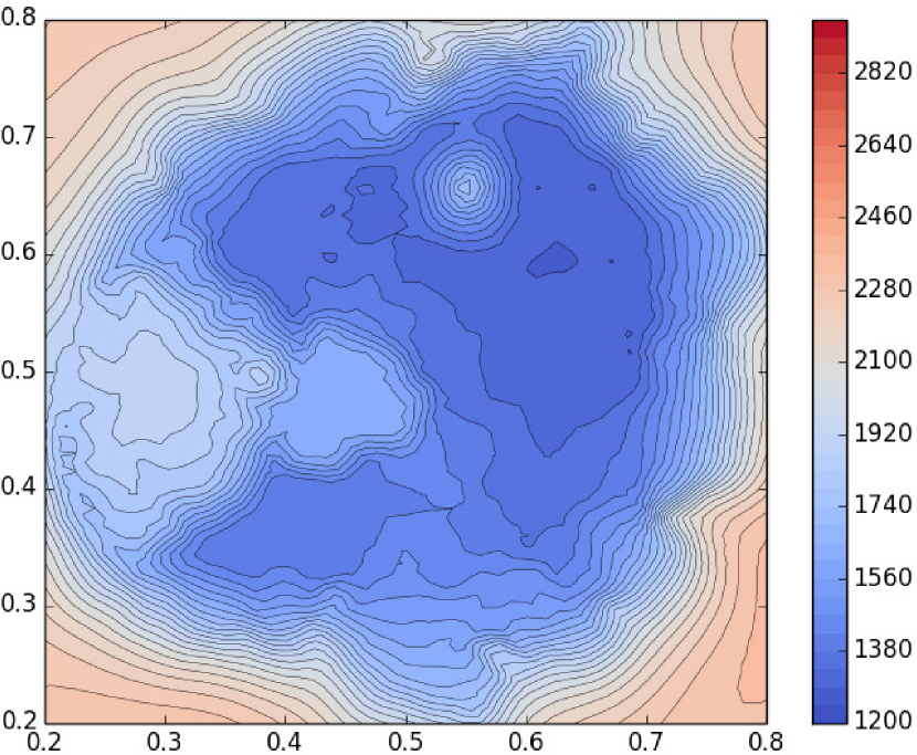
(a)

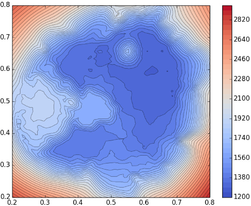
(b)

Figure 12: Contour plots of $s$ using a uniform grid of 8,321 nodes with (a) Dirichlet boundaries; and (b) Neumann boundaries.

There is an island on the Crater Lake near $\bm{x}=[0.3,0.5]$ as shown in Figure 12, and this region does not have any data points. Figure 13 compares the approximation in this region using uniform refinement (a) and adaptive refinement (b). Note the plots in Figure 13 are scaled differently compared to the plots in Figures 12 to better show the details. The plots were obtained using the auxiliary problem error indicator. Although, as discussed in Section 4.2, this error indicator depends on local data distributions, it is applicable to regions without data points. The resulting smoother shown in Figure 13(a) is similar to that obtained using a uniform grid shown in Figure 13(b).

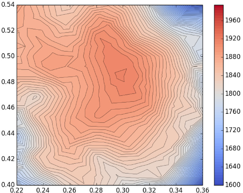
(a)

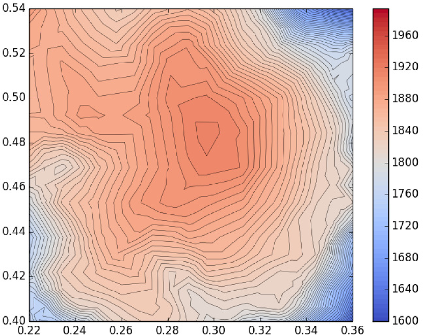
(b)

Figure 13: Contour plots of $s$ in a small region without data points using (a) uniform refinement; and (b) adaptive refinement.

The Crater lake data set consists of oscillatory and smooth regions. The contour maps of the Crater Lake data of two example oscillatory regions on an underwater hill and near shorelines are provided in Figures 14(a) and 14(b), respectively. Areas with white space represent regions without data points. The peak of the underwater hill sits near the point [0.55,0.65] in Figure 12. Figure 14(b) shows rapid changes in heights near a shoreline. In contrast, the lower right corner in Figure 14(b) is a smooth region.

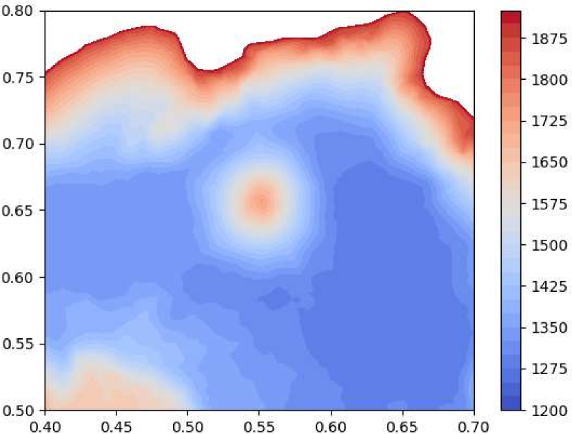
(a)

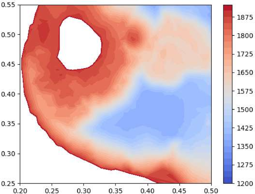
(b)

Figure 14: Contour maps for Crater Lake data at (a) underwater hill; and (b) shoreline. White spaces represent regions without data points.

Figure 15 shows the parts of the adaptive grid corresponding to the data plots in Figure 14. This is the adaptive grid constructed using the norm-based error indicator. Observe the oscillatory regions are refined to improve the accuracy of the FEM approximation. In Figure 15(a), finer elements are evident near the peak of the underwater hill that sits near the point [0.55,0.65]. In contrast, the lower right corner has coarser elements. Similarly, shorelines in Figure 15(b) have finer elements compared to the bottom of the lake at the bottom right corner. An example adaptive grid of the whole domain is shown in Figure 17(a).

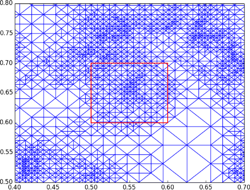
(a)

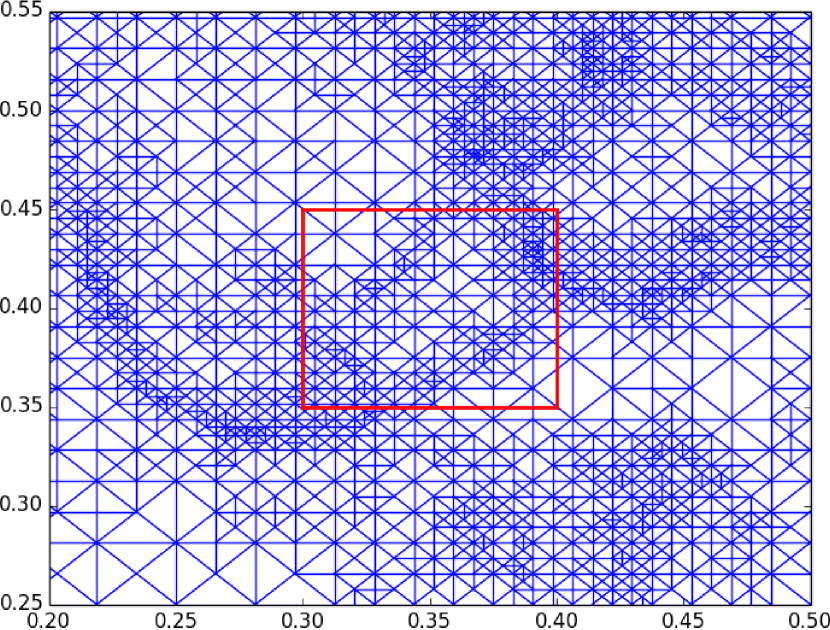
(b)

Figure 15: Adaptive grids for Crater Lake at (a) underwater hill; and (b) shoreline. The underwater hill and shoreline are highlighted by red squares in subfigures (a) and (b), respectively.

The convergence of the RMSE of the TPSFEM using uniform and adaptive grids for the Crater lake survey with Dirichlet and Neumann boundaries is shown in Figures 16(a) and 16(b), respectively. We applied the same initial grid and refinement setting used in Section 5.1. Statistics of refined grids for the Crater Lake data are provided in Table 3. The adaptive grids produced by the four error indicators with Dirichlet boundaries have similar error convergence rates, which are significantly higher than that of the uniform grid as shown in Figure 16(a). Apart from the auxiliary problem error indicator with Neumann boundaries, the adaptive grids achieve lower RMSE compared to the uniform grids using about $39.21\%$ of the number of nodes and about $47.62\%$ of solve time for Dirichlet boundaries; and about $39.04\%$ of the number of nodes and about $44.68\%$ of solve time for Neumann boundaries as shown in Table 3.

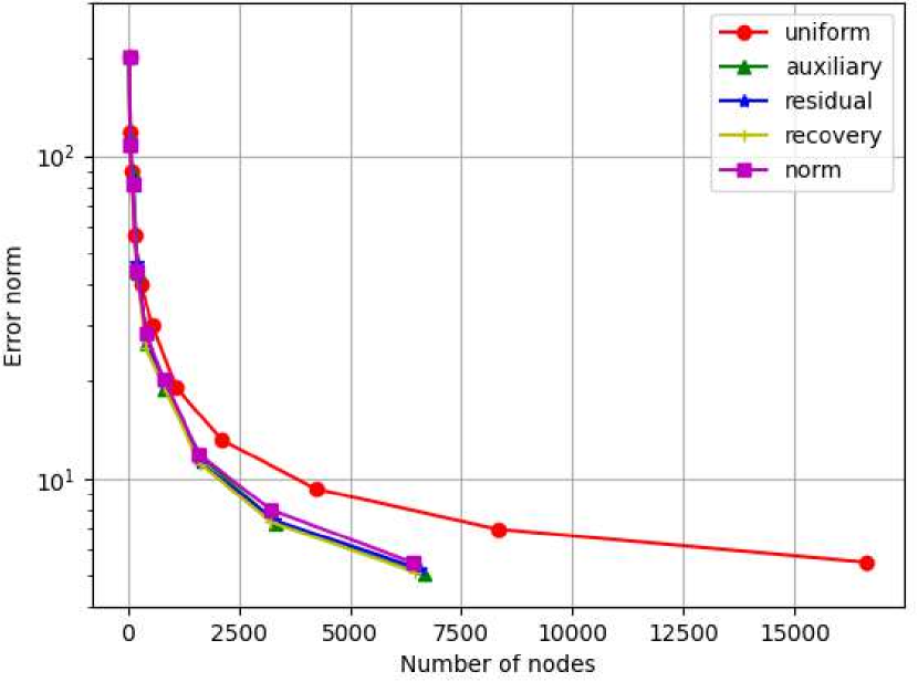
(a)

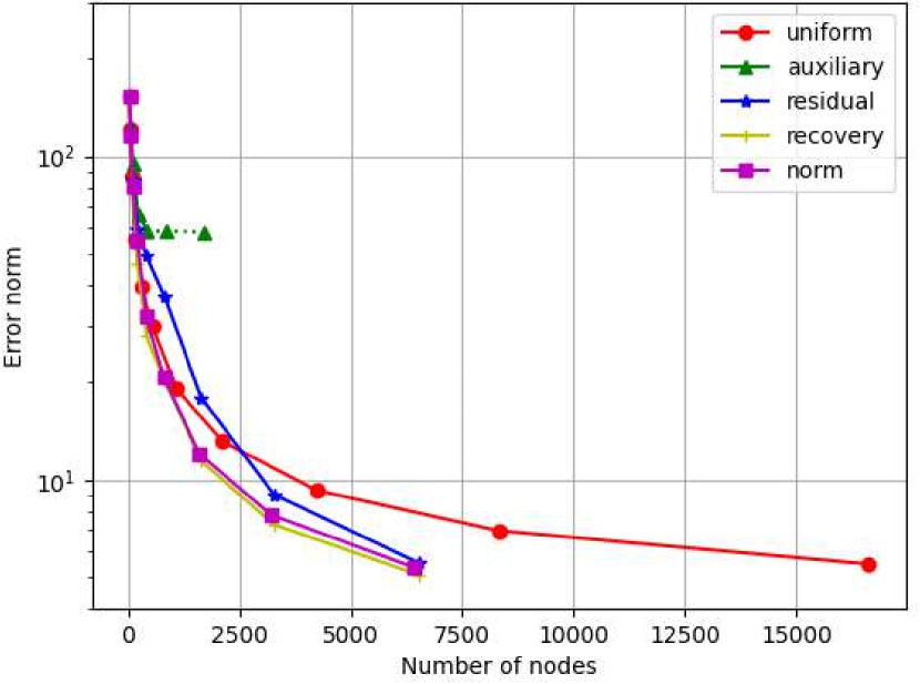
(b)

Figure 16: RMSE of TPSFEM using uniform and adaptive grids with (a) Dirichlet boundaries; and (b) Neumann boundaries.

Table 3: Regression metrics of the TPSFEM for Crater Lake data

Boundary	Metric	Uniform	Auxiliary	Residual	Recovery	Norm
Dirichlet	RMSE	5.50	5.06	5.25	5.14	5.50
	RMSPE	$2.92\times 10^{-3}$	$2.72\times 10^{-3}$	$2.82\times 10^{-3}$	$2.76\times 10^{-3}$	$2.95\times 10^{-3}$
	MAX	106.12	107.19	104.16	102.63	104.78
	# nodes	16641	6676	6563	6450	6408
	Time	0.42	0.22	0.19	0.19	0.20
Neumann	RMSE	5.50	58.39	5.53	5.09	5.38
	RMSPE	$2.92\times 10^{-3}$	$0.03$	$2.97\times 10^{-3}$	$2.72\times 10^{-3}$	$2.89\times 10^{-3}$
	MAX	106.86	366.04	114.21	112.07	105.12
	# nodes	16641	1707	6544	6544	6401
	Time	0.47	0.047	0.21	0.22	0.20

The recovery-based error indicator and norm-based error indicator perform similarly with both the Dirichlet and Neumann boundaries. However, as shown in Figure 16(b), the residual-based error indicator did not work as well for Neumann boundaries and the auxiliary problem error indicator did not converge.

Example adaptive grids obtained using the auxiliary problem error indicator with Dirichlet and Neumann boundaries are shown in Figure 17. With Dirichlet boundary conditions, this error indicator focuses on ridges and shorelines of the lake as illustrated in Figure 17(a). Compare Figure 17(a) with Figure 12. However, with Neumann boundary conditions all refinement is concentrated on the boundaries as shown in Figure 17(b). Given that the refinement concentrated on regions not containing any data points, the RMSE will remain high. Recall that the iterative process of the TPSFEM terminates when the RMSE is not reduced fast enough as shown in the stopping criteria on line 19 of Algorithm 1. Consequently, the adaptive refinement process terminated with high errors as shown in Table 3. We have argued that when using Neumann boundary conditions the data needs to be placed well within the domain. The data distribution shown in Figure 11 demonstrates that the FEM elements near the boundary in the initial coarse grid interact with the data points. The grid in Figure 11 contains $5\times 5$ nodes. We reran the above experiment with a different initial coarse grid, one containing $20\times 20$ nodes, and found that the over-refinement near the boundary disappeared and the resulting grid more closely resembled that in Figure 17(a).

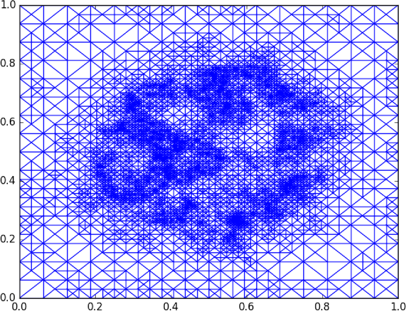
(a)

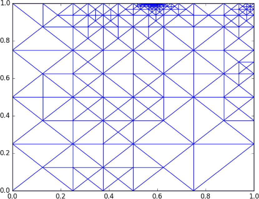
(b)

Figure 17: Adaptive grid using auxiliary problem error indicator with (a) Dirichlet boundaries; and (b) Neumann boundaries.

5.3 Results: Coastal region

With the Coastal Region data, we compared the performance of the TPSFEM in both the L-shaped domain and $[0,1]^{2}$ square domains. Similar to the Crater Lake data, the Coastal Region data was scaled so the data points fall inside the domain $[0.2,0.8]^{2}$. See Figure 18 for an example coarse grid used in the L-shaped domain. Note that we chose this scale since Coastal Region data has relatively small oscillations near $\bm{x}=[0.4,0.5]$. As the data values change drastically from the shore to nearby reefs, it is not possible to estimate appropriate values to accompany any Dirichlet boundary conditions. Therefore, we use zero Neumann boundaries.

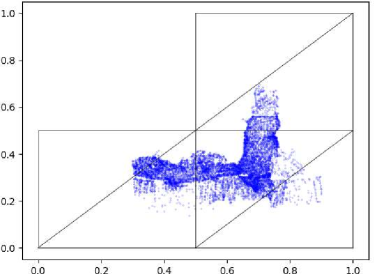
Figure 18: Randomly sampled data points in initial FEM grids for Coastal Region data. Data points are represented as blue dots.

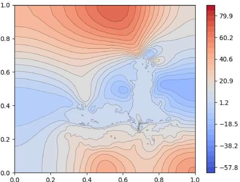
(a)

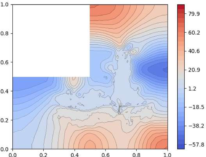
(b)

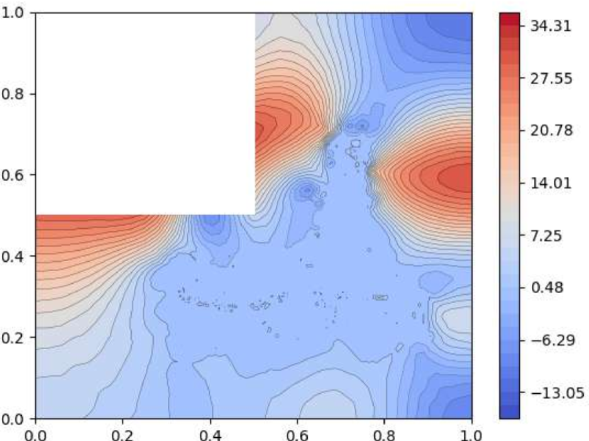
(c)

Figure 19: Contour plots of TPSFEM using auxiliary problem error indicator in (a) square domain; and (b) L-shaped domain. Contour plot of difference between these two smoothers within the L-shaped domain in (c). Note that Figure (c) is scaled differently to show more details.

Two contour plots of the approximations obtained using square and L-shaped domains for the Coastal Region data are shown in Figures 19(a) and 19(b), respectively. While both smoothers are similar in regions covered by the observed data, the approximation in the L-shaped domain has a steeper descent near the points $[0.2,0.5]$, $[0.5,0.7]$ and $[0.9,0.6]$ as illustrated in Figure 19(c). Note the scaling of Figure 19(c) is different from Figures 19(a) and 19(b) and was chosen to highlight the details.

The convergence of the RMSE of the TPSFEM using uniform and adaptive grids for the Coastal Region data using square and L-shaped domains is shown in Figures 20(a) and 20(b), respectively. The initial square and L-shaped grids contain 25 and 21 nodes, respectively. They are both refined using uniform and adaptive refinement for at most 10 and 8 iterations, respectively. Adaptive grids produced by the auxiliary problem and recovery-based error indicators achieve higher efficiency than ones of the residual-based and norm-based error indicators. Statistics of refined grids for the Coastal Region data are provided in Table 4. The adaptive grids have significantly higher error convergence rates compared to the uniform grid in both square and L-shaped domains. They achieve about $60.23\%$ of RMSE compared to the uniform grids using about $39.18\%$ of the number of nodes and about $47.78\%$ of solve time for square domains; and about $66.29\%$ of RMSE using about $44.21\%$ of the number of nodes and about $58.33\%$ of solve time for L-shaped domains as shown in Table 4. Moreover, the L-shaped domain improves the efficiency of adaptive grids for both uniform and adaptive refinement.

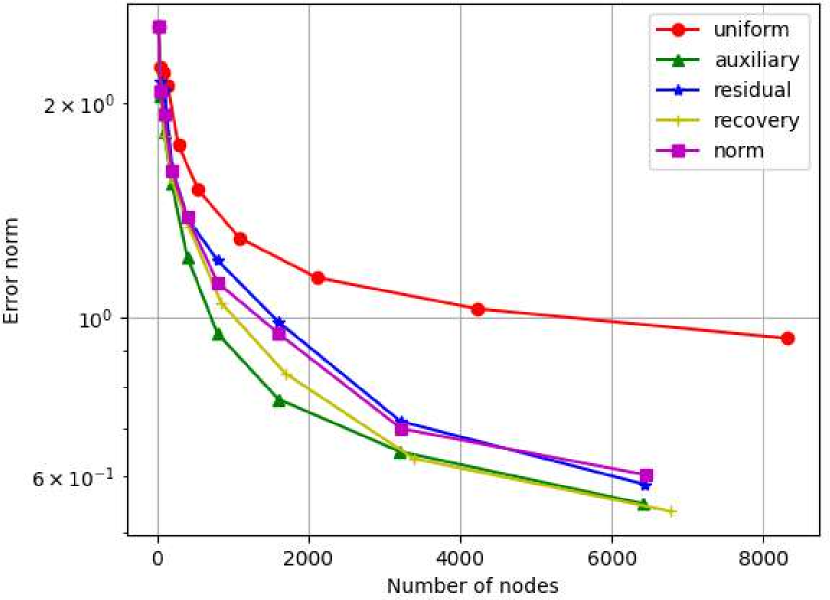
(a)

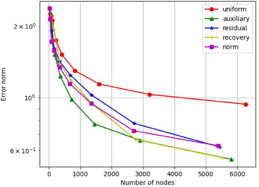
(b)

Figure 20: RMSE of TPSFEM using uniform and adaptive grids with (a) square domain; and (b) L-shaped domain.

Table 4: Regression metrics of the TPSFEM for Costal Region data

Domain	Metric	Uniform	Auxiliary	Residual	Recovery	Norm
Square	RMSE	0.88	0.58	0.55	0.54	0.55
	RMSPE	0.030	0.019	0.020	0.018	0.020
	MAX	12.51	7.07	7.12	6.17	7.07
	# nodes	16641	6416	6432	6786	6448
	Time	0.45	0.21	0.21	0.22	0.22
L-shaped	RMSE	0.89	0.55	0.62	0.56	0.63
	RMSPE	0.030	0.019	0.021	0.019	0.021
	MAX	12.60	7.02	7.08	6.22	6.36
	# nodes	12545	5818	5440	5528	5397
	Time	0.33	0.20	0.19	0.19	0.19

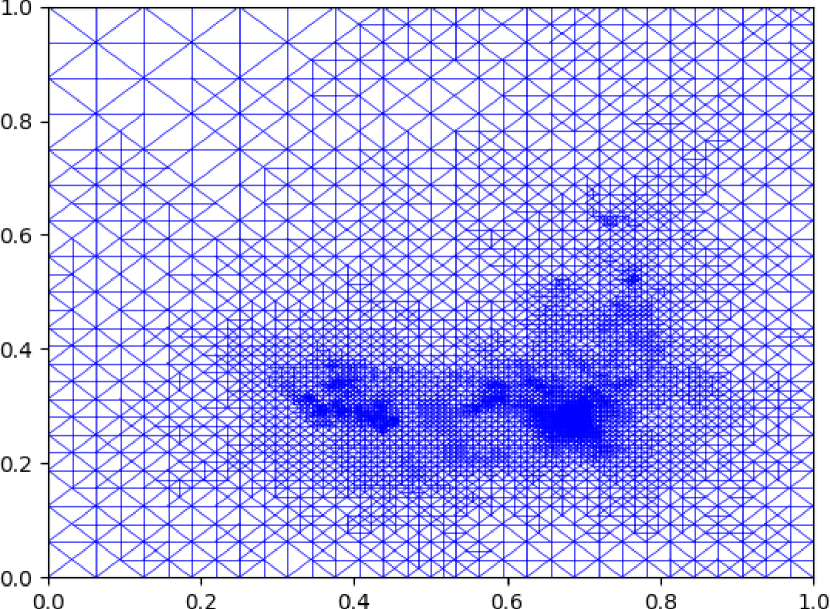
(a)

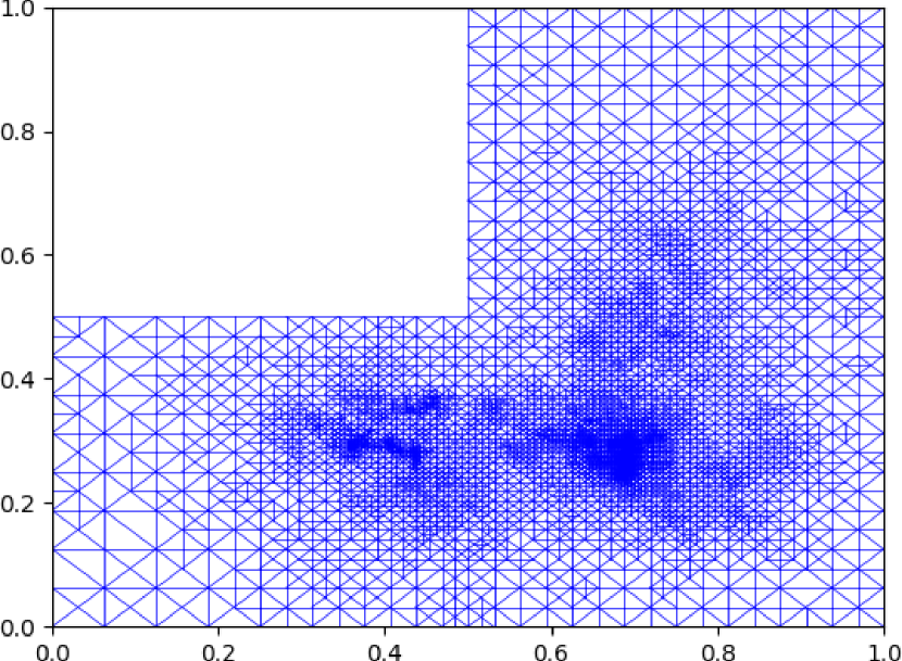
(b)

Figure 21: Adaptive grid using recovery-based error indicator with (a) square domain; and (b) L-shaped domain.

Two example adaptive grids produced using the recovery-based error indicator on the square and L-shaped domains are shown in figures 21(a) and 21(b), respectively. Refinement is concentrated at the bay area illustrated in Figure 18.

6 Conclusion

We formulated an adaptive refinement process for a FEM approximation of the thin plate spline. The FEM approximation is called the TPSFEM. We demonstrated this process needs to take into account not just the spacing of the FEM grid, as is standard with adaptive refinement techniques, but also the data distribution as well as the smoothing parameter in the thin plate spline. Given the estimated errors of the FEM approximation do not solely depend on the grid spacing, the usual stopping criteria will not work. Consequently, we provided a detailed description of a new iterative adaptive refinement process. This process adopts stopping criteria that are based on the rate of change of the root-mean-square error (RMSE). Also, a low-cost technique is used to update the smoothing parameter by using the parameter obtained in the previous iteration of the refinement process.

We studied five error indicators. One error indicator was based on the RMSE. We showed this error indicator should not be used as it is sensitive to noise in the data and leads to over-refinement. We concluded this approach is not worth considering further. The remaining four error indicators are based on examples developed for PDEs. They are the auxiliary problem error indicator, residual-based error indicator, recover-based error indicator and norm-based error indicator.

We conducted experiments using both Dirichlet and Neumann boundary conditions and the error indicators showed similar performance irrespective of the boundary conditions in most cases. The one exception was the auxiliary problem error indicator which overrefined near one of the boundaries of the FEM grid when using Neumann boundary conditions. Note that this problem did go away when we looked at another set of test problems with a finer initial coarse grid. The other three error indicators worked well with Neumann boundary conditions when the FEM grid is extended well past the position of the data points.

To evaluate the error indicators, we studied one model problem and two bathymetric surveys with varied boundaries and domains. The model problem is based on MATLAB’s peaks function. Here, the four PDE-based error indicators gave similar error convergence, which was markedly higher than that obtained when using uniform refinement. For the first bathymetric survey carried out on a crater lake, the four PDE-based error indicators again gave similar performance and are more efficient than uniform refinement when using Dirichlet boundary conditions. The auxiliary problem error indicator did not work well with Neumann boundary conditions, but the other three did. These experiments were carried out on a square domain. For the second bathymetric survey of a coastal region, both a square and an L-shaped domain were studied. Adaptive refinement outperformed uniform refinement in both domains. Additionally, the L-shaped domain improved the efficiency of the TPSFEM as the FEM grid contained fewer regions without data.

References

- [1] Z. Majdisova, V. Skala, Big geo data surface approximation using radial basis function: A comparative sutdy, Computers & Geosciences 109 (2017) 51–58. doi:10.1016/j.cageo.2017.08.007.
- [2] S. Roberts, M. Hegland, I. Altas, Approximation of a thin plate spline smoother using continuous piecewise polynomial functions, SIAM Journal on Numerical Analysis 41 (1) (2003) 208–234. doi:10.1137/S0036142901383296.
- [3] W. F. Mitchell, A comparison of adaptive refinement techniques for elliptic problems, ACM Transactions on Mathematical Software (TOMS) 15 (4) (1989) 326–347. doi:10.1145/76909.76912.
- [4] T. Grätsch, K. J. Bathe, A posteriori error estimation techniques in practical finite element analysis, Computers & Structures 83 (4-5) (2005) 235–265. doi:10.1016/j.compstruc.2004.08.011.
- [5] M. V. Shcherbakov, A. Brebels, N. L. Shcherbakova, A. P. Tyukov, T. A. Janovsky, V. A. Kamaev, A survey of forecast error measures, World Applied Sciences Journal 24 (24) (2013) 171–176. doi:10.5829/idosi.wasj.2013.24.itmies.80032.
- [6] J. C. Carr, R. K. Beatson, J. B. Cherrie, T. J. Mitchell, W. R. Fright, B. C. McCallum, T. R. Evans, Reconstruction and representation of 3d objects with radial basis functions, in: Proceedings of the 28th annual conference on Computer graphics and interactive techniques, ACM, 2001, pp. 67–76. doi:10.1145/383259.383266.
- [7] J. Duchon, Splines minimizing rotation-invariant semi-norms in Sobolev spaces (1977) 85–100doi:10.1007/BFb0086566.
- [8] J. Cowan, R. Beatson, H. J. Ross, W. R. Fright, T. J. McLennan, T. R. Evans, J. C. Carr, R. G. Lane, D. V. Bright, A. J. Gillman, P. A. Oshurst, M. Titley, Practical implicit geological modelling, 2003, pp. 89–99.
- [9] M. F. Hutchinson, Interpolation of rainfall data with thin plate smoothing splines. part i: Two dimensional smoothing of data with short range correlation, Journal of Geographic Information and Decision Analysis 2 (2) (1998) 139–151. doi:10.1080/02693799508902045.
- [10] T. Ramsay, Spline smoothing over difficult regions, Journal of the Royal Statistical Society: Series B (Statistical Methodology) 64 (2) (2002) 307–319. doi:10.1111/1467-9868.00339.
- [11] Z. M. Chen, R. Tuo, W. L. Zhang, Stochastic convergence of a nonconforming finite element method for the thin plate spline smoother for observational data, SIAM Journal on Numerical Analysis 56 (2) (2018) 635–659. doi:10.1137/16M109630X.
- [12] L. Stals, S. Roberts, Smoothing large data sets using discrete thin plate splines, Computing and Visualization in Science 9 (3) (2006) 185–195. doi:10.1007/s00791-006-0033-x.
- [13] L. Stals, Efficient solution techniques for a finite element thin plate spline formulation, Journal of Scientific Computing 63 (2) (2015) 374–409. doi:10.1007/s10915-014-9898-x.
- [14] L. Fang, Error indicators and adaptive refinement of the discrete thin plate spline smoother, ANZIAM Journal 60 (2019) 33–51. doi:10.21914/anziamj.v60i0.14061.
- [15] G. Wahba, Spline models for observational data, Vol. 59, SIAM, 1990. doi:10.1137/1.9781611970128.
- [16] H. Wendland, Piecewise polynomial, positive definite and compactly supported radial functions of minimal degree, Advances in Computational Mathematics 4 (1) (1995) 389–396. doi:10.1007/BF02123482.
- [17] M. D. Buhmann, Radial functions on compact support, Proceedings of the Edinburgh Mathematical Society 41 (1) (1998) 33–46. doi:10.1017/S0013091500019416.
- [18] J. V. Gardener, P. Dartnell, 2000 Multibeam sonar survey of Crater Lake, Oregon - Data, GIS, images and movies, https://pubs.usgs.gov/dds/dds-72/index.htm, accessed: 2021-03-10 (2001).
- [19] S. Deparis, D. Forti, A. Quarteroni, A rescaled localized radial basis function interpolation on non-cartesian and nonconforming grids, SIAM Journal on Scientific Computing 36 (6) (2014) A2745–A2762. doi:10.1137/130947179.
- [20] H. Wendland, Computational aspects of radial basis function approximation, in: Studies in Computational Mathematics, Vol. 12, Elsevier, 2006, pp. 231–256. doi:10.1016/S1570-579X(06)80010-8.
- [21] R. K. Beatson, W. A. Light, Fast evaluation of radial basis functions: methods for two-dimensional polyharmonic splines, IMA Journal of Numerical Analysis 17 (3) (1997) 343–372. doi:10.1137/S0036141099361767.
- [22] L. Stals, Radial basis functions: comparison between compact basis and finite element basis (In preparation).
- [23] O. C. Zienkiewicz, R. L. Taylor, J. Z. Zhu, The finite element method: its basis and fundamentals, Elsevier, 2005. doi:10.1016/C2009-0-24909-9.
- [24] I. Babuvška, A. K. Aziz, On the angle condition in the finite element method, SIAM Journal on Numerical Analysis 13 (2) (1976) 214226. doi:10.1137/0713021.
- [25] L. Stals, Parallel multigrid on unstructured grids using adaptive finite element methods, Ph.D. thesis, The Australian National University (1995).
- [26] F. Naddei, M. Plata, V. Couaillier, F. Coquel, A comparison of refinement indicators for p-adaptive simulations of steady and unsteady flows using discontinuous galerkin methods, Journal of Computational Physics 376 (2019) 508–533. doi:https://doi.org/10.1016/j.jcp.2018.09.045.
- [27] L. Fang, Error estimation and adaptive refinement of finite element thin plate spline, Ph.D. thesis, The Australian National University (2021).
- [28] L. Fang, L. Stals, Adaptive finite element thin-plate spline with different data distributions, Springer.
- [29] G. H. Golub, M. Heath, G. Wahba, Generalized cross-validation as a method for choosing a good ridge parameter, Technometrics 21 (2) (1979) 215–223. doi:10.1080/00401706.1979.10489751.
- [30] M. F. Hutchinson, A stochastic estimator of the trace of the influence matrix for Laplacian smoothing splines, Communications in Statistics-Simulation and Computation 19 (2) (1990) 433–450. doi:10.1080/03610919008812866.
- [31] L. Fang, L. Stals, Adaptive discrete thin plate spline smoother, ANZIAM Journal 62 (2021) 45–57. doi:10.21914/anziamj.v62.15979.
- [32] R. P. Brent, Algorithms for minimization without derivatives, Courier Corporation, 2013. doi:10.1109/TAC.1974.1100629.
- [33] M. Ainsworth, J. T. Oden, A posteriori error estimation in finite element analysis, Vol. 37, John Wiley & Sons, 2011. doi:10.1016/S0045-7825(96)01107-3.
- [34] I. Babuvška, W. C. Rheinboldt, Error estimates for adaptive finite element computations, SIAM Journal on Numerical Analysis 15 (4) (1978) 736–754. doi:10.1137/0715049.
- [35] Q. Zhang, Y. Z. Zhao, J. Levesley, Adaptive radial basis function interpolation using an error indicator, Numerical Algorithms 76 (2) (2017) 441–471. doi:10.1007/s11075-017-0265-5.
- [36] O. C. Zienkiewicz, J. Z. Zhu, A simple error estimator and adaptive procedure for practical engineerng analysis, International Journal for Numerical Methods in Engineering 24 (2) (1987) 337–357. doi:10.1002/nme.1620240206.
- [37] C. Carstensen, S. Funken, Averaging technique for FE – a posteriori error control in elasticity. Part ii: -independent estimates, Computer Methods in Applied Mechanics and Engineering 190 (2001) 4663–4675. doi:10.1016/S0045-7825(00)00338-8.
- [38] E. G. Sewell, Analysis of a finite element method: PDE/PROTRAN, Springer Science & Business Media, 2012. doi:10.1007/978-1-4684-6331-6.
- [39] J. Terrano, K. Smith, A. Muni-Morgan, N. Buster, F. Foxen, Historical bathymetry in the Mississippi-Alabama coastal region: Bathymetric soundings, gridded digital elevation model, and hydrographic sheets (ver. 2.0, march 2022), https://coastal.er.usgs.gov/data-release/doi-P9GRUK4B/, accessed: 2021-011-3 (2021). doi:10.5066/P9GRUK4B.