A Machine Learning Method for Stackelberg Mean Field Games

Abstract

In this paper, we propose a single-level numerical approach that uses machine learning techniques to solve bi-level Stackelberg problems between a principal and a mean field of agents. In Stackelberg mean field games, there is an infinite population of agents who play a non-cooperative game and choose their controls to optimize their individual objectives while interacting with the principal and other agents through the population distribution. The principal can influence the mean field game Nash equilibrium at the population level through policies, and she aims at optimizing her own objective, which depends on the population distribution. This leads to a bi-level problem between the principal and mean field of agents that cannot be solved using traditional methods for mean field games. We propose a reformulation of this problem as a single-level mean field optimal control problem through a penalization approach. We prove convergence of the reformulated problem to the original problem. We then propose a numerical method based on neural networks and illustrate it on several examples from the literature.

Keywords. mean field games, Stackelberg equilibrium, Nash equilibrium, contract theory, deep learning

AMS subject classifications. 49N90, 91A13, 91A15, 62M45.

Acknowledgments. The authors would like to thank René Carmona for helpful discussions.

1 Introduction

In policy making, finding optimal policies to solve socioeconomic problems is the ultimate goal. However, this problem has an underlying complexity: Individualistic nature of humankind prevents policy makers to directly control the behavior of people. Instead, the policymakers should take into account the reaction of the society – consisting of non-cooperative agents – to a policy while deciding on the best one. One approach to understand the emergent reactions to any given policy can be to use simulation techniques such as agent-based simulation, which is commonly used for modeling complex interactions among agents. However, it lacks the tractability of the solutions. This lack of tractability issue prevents us from solving for optimal policies. Instead, with this approach only the outcomes of different policies can be compared. Therefore, in order to attain tractability of the solutions when there are many agents interacting with each other, we can utilize game theoretical tools such as mean field games (MFGs). Intuitively, in the MFG setup, we focus on a game among a large number of indstinguishable agents that are interacting symmetrically. Then, we study the equilibrium between a representative player and the distribution of the other players’ states (and possibly actions) instead of focusing on the interactions of every player with each other. With this simplification, we can characterize an approximate Nash equilibrium in the society given an policy (i.e., incentive or contract) by using forward-backward differential equations. Even if this forward-backward system could be hard to analyze, mean field equilibria are simpler to identify and compute than equilibria of populations with finite but large number of agents because of the curse of dimensionality. The mean field equilibria provide approximate Nash equilibria for games with a large but finite number of players.

After finding a tractable solution for the non-cooperative game (i.e., Nash equilibrium) of large number of agents given any policy by using MFG approach, our second step is to find the optimal policy. This can be done by the addition of a principal to the model who has her own objectives (different than the objectives of the agents in the society) and chooses policies in order to affect the Nash equilibrium in the society. The addition of this principal changes our problem from a standard MFG to a Stackelberg MFG between a principal and a mean field population of agents. This Stackelberg MFG problem is a bi-level problem where we look for the mean field equilibrium in the society given any policy at the population level and optimize the policy of the principal by taking into account this equilibrium reaction from the society at the top level. Mathematically, this corresponds to solving an optimal control problem that is constrained by an MFG equilibrium.

In this paper, we focus on writing the Stackelberg MFG problem as a single level optimal control problem and proposing a numerical approach to solve Stackelberg MFG in a general setting.

1.1 Literature review

1.1.1 Mean field games

When there is a large number of agents in a game setting, computing a Nash equilibrium is a daunting task because of the exponentially increasing number of interactions among the agents. The MFG approach was proposed in [31] and [33, 34] simultaneously and independently to overcome theses challenges. In MFGs, it is assumed that there is infinitely many indistinguishable agents interacting in a symmetric way. The agents do not directly see the state or the action of another specific agent. Instead, each agent sees the population distribution of states (or controls or joint distribution of states and controls). In the mean-field regime, Nash equilibria can be characterized by a system of forward-backward equations. In the analytical approach, the system consists of two partial differential equations (PDEs): a Hamilton-Jacobi-Bellman and a Kolmogorov-Fokker-Plank equations. In the probabilistic approach, the system consists of two stochastic differential equations, and the system is referred to as a forward-backward stochastic differential equation (FBSDE) system. Interested readers can refer to the books [8, 14].

1.1.2 Contract theory and Stackelberg mean field games

Contract theory studies the interaction between a principal and an agent. The principal proposes a contract to the agent and the agent reacts to the given contract so as to minimize his cost (or, equivalently, to maximize her reward). For example, the agent can decide how much effort he will put in the work while working for the principal. For a given contract, the agent needs to solve an optimal control problem. The goal of the principal is to find the best contract to minimize her own cost (or to maximize her own reward). Solutions to contract theory problems are generally studied using the notion of Stackelberg equilibrium. In [27] continuous time method is used to study this type of problems, and in [39, 40] dynamic programming and martingale optimality principles are used to characterize the solution. These ideas are later generalized in [19]. In [21] the solution in a general class of principal agent problem is characterized by using the Pontryagin stochastic maximum principle.

In the model we consider in this paper, instead of having one principal and one agent, we have a population of large number of agents and we will model the large number of agents with a mean field game. In our setup, the principal tries to optimize her policies by taking the mean field Nash equilibrium reaction of the population to the given policy. This creates a Stackelberg equilibrium between the principal and the mean field of agents. In the context of MFGs, problems with a principal and a mean field of agents have been studied in [22] in the continuous state space setting and in [17] for finite state spaces. Linear-quadratic models have received particular attention for their tractability, see e.g. [6, 36, 35]. Stackelberg MFG approach is used to find equilibrium in many applications such as optimal advertisement decisions [38, 12], epidemic control [5] or optimal carbon tax regulations [13]. The theory has been extended to cover problems with delay in [7] or problems with a collaborative population [32], which corresponds to Stackelberg equilibrium between a principal and another player with McKean-Vlasov dynamics. [30] considered a model with a single agent and a mean field of principals. Last, Stackelberg MFG should be distinguished from major-minor MFGs, which usually refer to a situation in which one player interacts with a mean field of infinitesimal agents and the whole situation is described as a Nash equilibrium among all the players. Interested readers can refer to [15, Chapter 7.1]. In [12] the differences between Stackelberg mean field games and major-minor mean field games are discussed in an advertisement competition application with multiple major players.

1.1.3 Numerical approaches in Stackelberg MFGs

Even though MFGs provide a simplified way to find approximate equilibria in games with finite but large number of agents, the forward-backward differential equation systems characterizing the mean field Nash equilibrium are still difficult to solve. Explicit solutions are available only in very few cases, such as in linear-quadratic MFGs. However, these models are not sufficient to capture the complexity of real life problems. On top of this difficulty, adding the optimization of the principal in the model introduces another level of optimization to our problem and in general the solution cannot be characterized using a classical PDE or FBSDE system. As a consequence, we cannot rely directly on traditional numerical methods for MFGs based on solving PDEs or FBSDEs [2, 1, 9, 11, 18, 4] (see also [3] for a recent survey). Therefore, new numerical approaches needs to be developed to solve Stackelberg MFG problems.

Recently, a few works have considered numerical approaches for specific classes of Stackelberg MFGs. In [5], the authors are motivated by finding the optimal time dependent social distancing policies and path dependent stimulus payment to mitigate an epidemic and model the government as the principal and the people in the society as the mean field game population. In this paper, building on the method proposed in [16], a numerical approach that uses deep learning tools and Monte Carlo simulation is proposed to solve finite state Stackelberg MFG as a single-level optimization problem. However, this approach required a specific relationship between the terminal costs of principal and the agents. In [10], authors propose a deep learning method to solve Stackelberg MFG problem where the principal chooses only the terminal payment structure among piecewise-linear function set. With this simplification, they solve bi-level Stackelberg MFG where they fix a control for the principal and solve the equilibrium and then optimize over the control set of the principal. In this work, we propose a method that can tackle a much wider class of Stackelberg MFGs, in terms of cost functions and dynamics.

1.2 Contributions and paper structure

The main contributions of this paper are three-fold. First, we propose a general approach which is based on rephrasing the Stackelberg MFG as a single-level optimal control problem driven by SDEs instead of the original formulation involving bi-level optimization. Roughly speaking, the proposed approach relies on a penalty to merge the Nash equilibrium constraint with the principal’s cost, and on the approximation of the controls using parameterized functions. Second, we provide a theoretical foundation to our approach by proving convergence results in terms of the penalization and the function approximation. Third, we provide numerical experiments on several examples from the literature. In particular, even if we give the continuous space setup in our paper, our approach is suitable for both continuous and finite space models with general cost functions.

In Section 2, we introduce the model setting and the analysis of the model. Furthermore, we rewrite the Stackelberg MFG model as a single-level optimal control problem. In Section 3, we prove the convergence of the solution of rewritten optimization problem to the original problem and give results on the convergence of the numerical approach that is introduced in Section 4. In Section 4, we give details of our numerical approach and discuss some extensions in Section 4.2. In Section 5, we evaluate the proposed numerical approaches with different models with applications to contract theory and systemic risk problems.

2 Model

In this section, we introduce the mathematical model for the Stackelberg MFG. We analyze the solution of the mean field game given the policies of the principal. In the last subsection, we rewrite the bi-level Stackelberg MFG problem as a single-level problem.

2.1 Preliminaries and notation

We adopt the following notation throughout the paper. Let $T>0$ be a finite time horizon. We assume that the problem is set on a complete filtered probability space $(\Omega,\mathcal{F},\mathbb{F}=(\mathcal{F}_{t})_{t},\mathbb{P})$ supporting a $d$-dimensional Wiener process $\boldsymbol{W}=(W_{t})_{t\in[0,T]}$. The representative infinitesimal agent has an $m$-dimensional continuous state process $\boldsymbol{X}=(X_{t})_{t\in[0,T]}$ where $X_{t}\in\mathbb{R}^{{m}}$ for all $t\in[0,T]$. We endow $\mathcal{P}(\mathbb{R}^{m})$, the space of probability measures on $\mathbb{R}^{m}$, with the 2-Wasserstein distance denoted by $W_{2}$ and defined as:

$$W_{2}(\mu,\nu):=\inf_{\pi\in\Pi(\mu,\nu)}\left[\int_{\mathbb{R}^{m}\times\mathbb{R}^{m}}d(x,y)^{2}d\pi(dx,dy)\right]^{1/2},$$ (2.1)

where $\Pi(\mu,\nu)$ denotes the set of probability measures in $\mathcal{P}(\mathbb{R}^{m}\times\mathbb{R}^{m})$ with marginals $\mu$ and $\nu$. Let $M(\mathcal{P}(\mathbb{R}^{{m}}))$ be the set of measurable mappings from $[0,T]$ to $\mathcal{P}(\mathbb{R}^{{m}})$. We denote the collection of square-integrable and $\mathbb{F}$-measurable action processes $\boldsymbol{\alpha}=(\alpha_{t})_{t\in[0,T]}$ with $\mathbb{A}$. The action space is denoted by $A$ is a subset of $\mathbb{R}^{k}$ i.e., $\alpha_{t}\in A\subset\mathbb{R}^{k}$.

Furthermore, given the complete filtered probability space $(\Omega,\mathcal{F},\mathbb{F},\mathbb{P})$, we denote by $\mathcal{H}^{2,n}$ the set of $\mathbb{F}$-adapted and real-valued processes

$$\mathcal{H}^{2,n}=\left\{\boldsymbol{Z}\in\mathcal{H}^{0,n}:\mathbb{E}\int_{0}^{T}|Z_{s}|^{2}ds<\infty\right\},$$

where $\mathcal{H}^{0,n}$ is the collection of all $\mathbb{R}^{n}$-valued measurable processes on [0,T].

2.2 General setting for Stackelberg mean field game

We consider an infinite population of non-cooperative players and one principal. Since the population of non-cooperative players is infinite, each player has a negligible influence on the rest of the population. The infinitesimal agents are influenced by the actions of the principal, which can be thought of as a regulator who can influence the Nash equilibrium of the mean field population. We begin by focusing on the game between the members of the population. As is common in the MFG paradigm, we focus on a representative player. Given knowledge of how the population and the principal act over time, the representative player optimizes their cost functional.

Let $\Lambda$ be the set of possible actions for the principal. Although more general sets could be considered, to simplify the presentation, we will use $\Lambda=\mathbb{R}$ and we consider policies that are elements of $C^{0}([0,T];\mathbb{R})$, which is the set of real-valued continuous functions of time. Assume the principal has chosen policy $\boldsymbol{\lambda}=(\lambda(t))_{t\in[0,T]}\in C^{0}([0,T];\Lambda)$, and the flow of population distribution is given by $\boldsymbol{\mu}=(\mu_{t})_{t\in[0,T]}\in M(\mathcal{P}(\mathbb{R}^{{m}}))$. Consider an infinitesimal agent using control $\boldsymbol{\alpha}=(\alpha_{t})_{t\in[0,T]}\in\mathbb{A}$. Then, the state of this agent is described by an $m$-dimensional stochastic process $\boldsymbol{X}$ which has the following dynamics:

$$dX_{t}=b(t,X_{t},\alpha_{t},\mu_{t};\lambda(t))dt+\sigma dW_{t},\qquad X_{0}=\zeta,$$ (2.2)

where $b:[0,T]\times\mathbb{R}^{m}\times A\times\mathcal{P}(\mathbb{R}^{{m}})\times\Lambda\to\mathbb{R}^{{m}}$ is the drift of the agent’s state process that depends on the agent’s own state $X_{t}$, her own action $\alpha_{t}$, the mean field distribution $\mu_{t}$ and the principal’s policy $\lambda(t)$. $\sigma>0$ is a constant volatility and $\boldsymbol{W}=(W_{t})_{t\in[0,T]}$ is a $d$-dimensional Wiener process that represents the idiosyncratic noise. The initial condition of the state process is denoted by $\zeta\in L^{2}(\Omega,\mathcal{F}_{0},\mathbb{P};\mathbb{R}^{{m}})$ and has distribution $\mu_{0}=\mathcal{L}(\zeta)$, which is also the initial state distribution of the population.

The representative player pays the expected total cost:

$$J^{\boldsymbol{\lambda}}(\boldsymbol{\alpha},\boldsymbol{\mu}):=\mathbb{E}\left[\int_{0}^{T}f(t,X_{t},\alpha_{t},\mu_{t};\lambda(t))dt+g(X_{T},\mu_{T};\lambda(T))\right],$$ (2.3)

where $f:[0,T]\times\mathbb{R}^{m}\times A\times\mathcal{P}(\mathbb{R}^{{m}})\times\Lambda\to\mathbb{R}$ is a running cost which depends on the agent’s own state $X_{t}$, her own action $\alpha_{t}$, the mean field distribution $\mu_{t}$, and the principal’s policy $\lambda(t)$. Finally, $g:\mathbb{R}^{m}\times\mathcal{P}(\mathbb{R}^{{m}})\times\Lambda\to\mathbb{R}$ is the terminal cost of the agent and it depends on the agent’s own state, the mean field distribution, and the principal’s policy at the terminal time.

We stress that the representative player interacts with the population through the mean field distributions $\boldsymbol{\mu}=(\mu_{t})_{t\in[0,T]}$ in the running cost, terminal cost and the drift of the state dynamics and interacts with the principal through the policy of the principal $\boldsymbol{\lambda}=(\lambda(t))_{t\in[0,T]}$ in the running cost, terminal cost and the drift of the state dynamics. Now, we can define the equilibrium in the mean field population given the principal’s policy selection.

Definition 2.1.

Let $\boldsymbol{\lambda}\in C^{0}([0,T];\mathbb{R})$ be a policy of the principal. We say that $(\boldsymbol{\hat{\alpha},\hat{\mu}})\in\mathbb{A}$ is a mean field Nash equilibrium given the policy $\boldsymbol{\lambda}$ if the following two conditions are met:

• $\boldsymbol{\hat{\alpha}}=\arg\inf_{\boldsymbol{\alpha}\in\mathbb{A}}J^{\boldsymbol{\lambda}}(\boldsymbol{\alpha},\boldsymbol{\hat{\mu}})$;

• For all $t\in[0,T]$, $\hat{\mu}_{t}=\mathcal{L}(X_{t})$, where $\boldsymbol{X}$ has dynamics (2.2) with control $\boldsymbol{\hat{\alpha}}$.

We denote by $\mathcal{N}(\boldsymbol{\lambda})$ the set of mean field Nash equilibria.

Intuitively, the first condition in Definition 2.1 states that the representative player finds her best response given the population state distribution and the second condition says that since the players are identical, the distribution of the representative player’s state induced by her best response control should correspond to the population state distribution fixed at the beginning.

The principal’s problem is to find the policies that create the most favorable reaction of the agents to minimize the principal’s own cost. By using policy $\boldsymbol{\lambda}$ as an incentive, the principal can affect the set of mean-field Nash equilibria $\mathcal{N}(\boldsymbol{\lambda})$ and in this way she can influence the population’s behavior to minimize her own cost.

Definition 2.2.

A policy of the principal $\boldsymbol{\lambda}$ is admissible if, given the deterministic mapping $\boldsymbol{\lambda}$, $\mathcal{N}(\boldsymbol{\lambda})$ is a singleton. We denote by $\boldsymbol{\Lambda}\subseteq C^{0}([0,T];\mathbb{R})$ the set of admissible policies.

Remark 2.3.

One of the ways to ensure uniqueness is to assume Lasry-Lions monotonicity [33, 34]. Interested readers can refer to [14, Theorem 3.32] for assumptions that yield uniqueness of the solution in MFG problems.

In order to use an admissible policy $\boldsymbol{\lambda}\in\boldsymbol{\Lambda}$ the principal pays the cost:

$$J^{0}(\boldsymbol{\lambda}):=\int_{0}^{T}f_{0}(t,\hat{\mu}^{\boldsymbol{\lambda}}_{t},\lambda(t))dt+g_{0}(\hat{\mu}_{T}^{\boldsymbol{\lambda}},\lambda(T))$$ (2.4)

where $(\boldsymbol{\hat{\alpha}}^{\boldsymbol{\lambda}},\boldsymbol{\hat{\mu}}^{\boldsymbol{\lambda}})=\mathcal{N}(\boldsymbol{\lambda})$. In this way, the principal’s optimization problem is:

$$\inf_{\boldsymbol{\lambda}\in\boldsymbol{\Lambda}}J^{0}(\boldsymbol{\lambda}).$$ (2.5)

Remark 2.4.

The principal’s objective is not just merely minimizing her own cost. The principal also needs to satisfy the constraint that the population is reacting the policy with a Nash equilibrium behavior. Because of this, our problem becomes a dynamic optimal control problem that is constrained by a Nash equilibrium condition. As we will see below, this constraint can be expressed in terms of a forward-backward system of stochastic differential equations (SDEs). The full problem is given in Subsection 2.4.

2.3 Analysis of the mean field game

In this section, before discussing the full problem between the principal and the mean field population, we first analyze the mean field game in the population. We characterize the Nash equilibrium in the mean field population given a policy of the principal, $\boldsymbol{\lambda}$, and give an existence result for the mean field Nash equilibrium.

Given a policy $\boldsymbol{\lambda}\in\boldsymbol{\Lambda}$ and the mean field interactions $\boldsymbol{\mu}$, the Hamiltonian for the representative player’s optimal control problem is given by the function $H:[0,T]\times\mathbb{R}^{{m}}\times\mathcal{P}(\mathbb{R}^{{m}})\times\mathbb{R}^{{m}}\times A\times\Lambda\mapsto\mathbb{R},$

$$H(t,x,\mu,\gamma,\alpha;\lambda):=b(t,x,\alpha,\mu;\lambda)\cdot\gamma+f(t,x,\alpha,\mu;\lambda).$$ (2.6)

The minimizer of the Hamiltonian is denoted by $\hat{\alpha}_{t}(x,\mu,\gamma;\lambda)$. In other words, we have:

$$\hat{\alpha}_{t}(x,\mu,\gamma;\lambda)=\operatorname*{arg\,min}_{\alpha}H(t,x,\mu,\gamma,\alpha;\lambda).$$ (2.7)

In order to characterize the Nash equilibrium in the MFG, we follow the analysis in [14, Chapter 4.4].

Assumption 2.5.

We assume:

1. $b$ and $f$ are measurable mappings from $[0,T]\times\mathbb{R}^{m}\times A\times\mathcal{P}(\mathbb{R}^{m})\times\Lambda$ into $\mathbb{R}^{m}$ and $\mathbb{R}$, respectively. $g$ is a measurable function from $\mathbb{R}^{m}\times\mathcal{P}(\mathbb{R}^{m})\times\Lambda$ into $\mathbb{R}$.

2. For all $(t,x,\alpha,\mu,\lambda)\in[0,T]\times\mathbb{R}^{m}\times A\times\mathcal{P}(\mathbb{R}^{m})\times\Lambda$, there exists a constant $L\geq 0$ such that

   $$|b(t,x,\alpha,\mu;\lambda)| \leq L(1+|\alpha|),$$ (2.8)

   $$|f(t,x,\alpha,\mu;\lambda)| \leq L(1+|\alpha|^{2}),$$

   $$|g(x,\mu;\lambda)| \leq L.$$

3. For any $t\in[0,T]$, $x\in\mathbb{R}^{m}$, $\mu\in\mathcal{P}(\mathbb{R}^{m})$ and $\lambda\in\Lambda$, the functions $b(t,x,\cdot,\mu;\lambda)$ and $f(t,x,\cdot,\mu;\lambda)$ are continuously differentiable in $\alpha$.

4. For any $t\in[0,T]$, $\alpha\in A$, $\mu\in\mathcal{P}(\mathbb{R}^{m})$ and $\lambda\in\Lambda$, the functions $b(t,\cdot,\alpha,\mu;\lambda)$, $f(t,\cdot,\alpha,\mu;\lambda)$, and $g(\cdot,\mu;\lambda)$ are L-Lipschitz continuous in x.

5. For any $t\in[0,T]$, $x\in\mathbb{R}^{m}$, $\alpha\in A$, and $\lambda\in\Lambda$, the functions $b(t,x,\alpha,\cdot;\lambda)$, $f(t,x,\alpha,\cdot;\lambda)$, and $g(x,\cdot;\lambda)$ are continuous in the measure argument with respect to the 2-Wasserstein distance.

6. For the same constant L and for all $(t,x,\alpha,\mu,\lambda)\in[0,T]\times\mathbb{R}^{m}\times A\times\mathcal{P}(\mathbb{R}^{m})\times\Lambda$,

   $$|\partial_{\alpha}b(t,x,\alpha,\mu;\lambda)| \leq L,$$ (2.9)

   $$|\partial_{\alpha}f(t,x,\alpha,\mu;\lambda)| \leq L.$$

7. There exists a unique minimizer $\hat{\alpha}_{t}(x,\mu,\gamma;\lambda)$ of the Hamiltonian $H(t,x,\mu,\gamma,\alpha;\lambda)$ given in (2.6). It is L-Lipschitz continuous in $(x,\gamma)$ and continuous in $\mu$ and satisfies: for all $(t,x,\alpha,\mu,\lambda)\in[0,T]\times\mathbb{R}^{m}\times A\times\mathcal{P}(\mathbb{R}^{m})\times\Lambda$,

   $$|\hat{\alpha}_{t}(x,\mu,\gamma;\lambda)|\leq L(1+|\gamma|).$$ (2.10)

Theorem 2.6.

If Assumption 2.5 holds, then for any initial condition $\zeta\in L^{2}(\Omega,\mathcal{F}_{0},\mathbb{P};\mathbb{R}^{{m}})$, the forward backward stochastic differential equation (FBSDE) system

$$X_{t} =\zeta+\int_{0}^{t}b(s,X_{s},\hat{\alpha}_{s}(X_{s},\mu_{s},{\sigma^{-1}}^{\top}Z_{s};\lambda(s)),\mu_{s};\lambda(s))ds+\int_{0}^{t}\sigma dW_{s}$$ (2.11)

$$Y_{t} =g(X_{T},\mu_{T};\lambda(T))+\int_{t}^{T}f(s,X_{s},\hat{\alpha}_{s}(X_{s},\mu_{s},{\sigma^{-1}}^{\top}Z_{s};\lambda(s)),\mu_{s};\lambda(s))ds-\int_{t}^{T}Z_{s}\cdot dW_{s}$$

with $\mu_{s}=\mathcal{L}(X_{s}),\ \forall s\in[0,T]$ is solvable and the flow given by the marginal distributions forward component of any solution is an equilibrium for the associated mean field game problem.

Proof.

Proof of Theorem 2.6. Introduce

$$B(t,x,\alpha,\mu) :=b(t,x,\alpha,\mu;\lambda(t)),$$

$$F(t,x,\alpha,\mu) :=F(t,x,\alpha,\mu;\lambda(t)),$$

$$\hat{a}_{t}(x,\mu,\gamma) :=\hat{\alpha}_{t}(x,\mu,\gamma;\lambda(t)),$$

$$G(x,\mu) :=g(x,\mu;\lambda(T))$$

Then the forward backward system in (2.11) can be written as

$$X_{t} =\zeta+\int_{0}^{t}B(s,X_{s},\hat{a}_{s}(X_{s},\mu_{s},{\sigma^{-1}}^{\top}Z_{s}),\mu_{s})ds+\int_{0}^{t}\sigma dW_{s}$$ (2.12)

$$Y_{t} =G(x,\mu)+\int_{t}^{T}F(s,X_{s},\hat{a}_{s}(X_{s},\mu_{s},{\sigma^{-1}}^{\top}Z_{s}),\mu_{s})ds-\int_{t}^{T}Z_{s}\cdot dW_{s}$$

The proof follows the same ideas given in [14, Chapter 4.4]. ∎

Remark 2.7.

We stress that the process $\boldsymbol{Y}$ in the FBSDE system (2.11) represents the value function of a representative agent.

2.4 Rewriting of the Stackelberg mean field game problem

As introduced in Subsection 2.2, we have a principal that minimizes her own cost by choosing policies for the infinitesimal agents in the population and by taking their reaction to these policies into account. In order to find the optimal policies of the principal, we need to find the mean field Nash equilibrium in the population given any chosen policy by the principal. Then the principal should optimize her policies by taking into account the equilibrium behavior of the society. This creates a bi-level problem where at the higher level the principal minimizes her own cost and at the lower level the mean field Nash equilibrium in the population is found. However, in order to implement an efficient numerical approach, we need to reduce this bi-level problem to a single level problem.

The bi-level problem is given as follows:

$$\left.\inf_{\begin{subarray}{c}\boldsymbol{\lambda}\in\boldsymbol{\Lambda}\end{subarray}}\int_{0}^{T}f_{0}(t,\mu_{t}^{\boldsymbol{\lambda}},\lambda(t))dt+g_{0}(\mu_{T}^{\boldsymbol{\lambda}},\lambda(T))\right\}\;\parbox{63.0001pt}{{\color[rgb]{0,0,0}\small Optimization of the Principal}}$$

$$\left.\begin{aligned} X_{t}^{\boldsymbol{\lambda}}&=\zeta+\int_{0}^{t}b(s,X_{s}^{\boldsymbol{\lambda}},\hat{\alpha}^{\boldsymbol{\lambda}}_{s},\mu_{s}^{\boldsymbol{\lambda}};\lambda(s))ds+\int_{0}^{t}\sigma dW_{s}\\ Y_{t}^{\boldsymbol{\lambda}}&=g(X^{\boldsymbol{\lambda}}_{T},\mu^{\boldsymbol{\lambda}}_{T};\lambda(t))+\int_{t}^{T}f(s,X_{s}^{\boldsymbol{\lambda}},\hat{\alpha}^{\boldsymbol{\lambda}}_{s},\mu_{s}^{\boldsymbol{\lambda}};\lambda(s))ds-\int_{t}^{T}Z_{s}^{\boldsymbol{\lambda}}\cdot dW_{s}\end{aligned}\right\}\;\parbox{63.0001pt}{{\color[rgb]{0,0,0}\small Equilibrium in\\ the Population}}$$

where $\mu_{t}^{\boldsymbol{\lambda}}=\mathcal{L}(X_{t}^{\boldsymbol{\lambda}})$ and $\hat{\alpha}_{s}^{\boldsymbol{\lambda}}:=\hat{\alpha}_{s}(X_{s}^{\boldsymbol{\lambda}},\mu_{s}^{\boldsymbol{\lambda}},{\sigma^{-1}}^{\top}Z_{s}^{\boldsymbol{\lambda}};\lambda(s))$.

As our first step, we write the backward SDE as a forward one and add a constraint to match the terminal condition of the backward SDE. In this way our problem can be written as

$$\inf_{\begin{subarray}{c}\boldsymbol{\lambda}\in\boldsymbol{\Lambda}\\ \boldsymbol{Z}\in\mathcal{H}^{2,m}\\ Y_{0}\end{subarray}}\int_{0}^{T}f_{0}(t,\mu_{t}^{\boldsymbol{\lambda},\boldsymbol{Z},Y_{0}},\lambda(t))dt+g_{0}(\mu_{T}^{\boldsymbol{\lambda},\boldsymbol{Z},Y_{0}},\lambda(T)),$$ (2.13)

with the constraint

$$Y_{T}^{\boldsymbol{\lambda},\boldsymbol{Z},Y_{0}}=g(X^{\boldsymbol{\lambda},\boldsymbol{Z},Y_{0}}_{T},\mu_{T}^{\boldsymbol{\lambda},\boldsymbol{Z},Y_{0}};\lambda(T)),$$ (2.14)

where the trajectories of $\boldsymbol{X}^{\boldsymbol{\lambda},\boldsymbol{Z},Y_{0}}$ and $\boldsymbol{Y}^{\boldsymbol{\lambda},\boldsymbol{Z},Y_{0}}$ are determined by the following forward forward stochastic differential equations:

$$X_{t}^{\boldsymbol{\lambda},\boldsymbol{Z},Y_{0}} =\zeta+\int_{0}^{t}b(s,X_{s}^{\boldsymbol{\lambda},\boldsymbol{Z},Y_{0}},\hat{\alpha}^{\boldsymbol{\lambda},\boldsymbol{Z},Y_{0}}_{s},\mu_{s}^{\boldsymbol{\lambda},\boldsymbol{Z},Y_{0}};\lambda(s))ds+\int_{0}^{t}\sigma dW_{s}$$ (2.15)

$$Y_{t}^{\boldsymbol{\lambda},\boldsymbol{Z},Y_{0}} =Y_{0}^{\boldsymbol{\lambda},\boldsymbol{Z},Y_{0}}-\int_{0}^{t}f(s,X_{s}^{\boldsymbol{\lambda},\boldsymbol{Z},Y_{0}},\hat{\alpha}^{\boldsymbol{\lambda},\boldsymbol{Z},Y_{0}}_{s},\mu_{s}^{\boldsymbol{\lambda},\boldsymbol{Z},Y_{0}};\lambda(s))ds+\int_{0}^{t}Z_{s}\cdot dW_{s},$$

where $\mu_{t}^{\boldsymbol{\lambda},\boldsymbol{Z},Y_{0}}=\mathcal{L}(X_{t}^{\boldsymbol{\lambda},\boldsymbol{Z}^{\boldsymbol{\lambda},\boldsymbol{Z},Y_{0}},Y_{0}^{\boldsymbol{\lambda},\boldsymbol{Z},Y_{0}}})$ and $\hat{\alpha}_{s}^{\boldsymbol{\lambda},\boldsymbol{Z},Y_{0}}:=\hat{\alpha}_{s}(X_{s}^{\boldsymbol{\lambda},\boldsymbol{Z},Y_{0}},\mu_{s}^{\boldsymbol{\lambda},\boldsymbol{Z},Y_{0}},{\sigma^{-1}}^{\top}Z_{s};\lambda(s))$.

The system given in (2.15) are the same equations given in (2.11) where the dynamic of $\boldsymbol{Y}$ is written in the forward direction in time. Hence, the terminal point of the adjoint process, $Y_{T}$, is going to be determined by the initial point chosen $Y_{0}$ and the coefficient $\boldsymbol{Z}$ in front of the Wiener process. In order to penalize any deviation from the terminal condition, $Y_{T}=g(X_{T},\mu_{T};\lambda(T))$, a penalty term is added to the cost function as a second step of the rewriting of the problem. When this penalty term is equal to 0, it is implied that the FBSDE is solved and in turn the solution of the FBSDE characterizes the mean field Nash equilibrium in the agent population.

Previously, the principal had $\boldsymbol{\lambda}$ as their control. However, as it is stated before now the terminal point of the adjoint process $Y_{T}$ is determined by $Y_{0}$ and $\boldsymbol{Z}$. Therefore, in the new optimal control problem, the controls are going to be $(\boldsymbol{\lambda},\boldsymbol{Z},Y_{0})$.

Now, we introduce a penalty for not satisfying the constraint and we rewrite the above constrained problem as follows:

$$\inf_{\begin{subarray}{c}\boldsymbol{\lambda}\in\boldsymbol{\Lambda}\\ \boldsymbol{Z}\in\mathcal{H}^{2,m}\\ Y_{0}\end{subarray}}\int_{0}^{T}f_{0}(t,\mu_{t}^{\boldsymbol{\lambda},\boldsymbol{Z},Y_{0}},\lambda(t))dt+g_{0}(\mu_{T}^{\boldsymbol{\lambda},\boldsymbol{Z},Y_{0}},\lambda(T))$$ (2.16)

$$\hskip 56.9055pt+\nu\mathbb{E}\left[\mathbf{P}\Big{(}Y^{\boldsymbol{\lambda},\boldsymbol{Z},Y_{0}}_{T}-g\big{(}X^{\boldsymbol{\lambda},\boldsymbol{Z},Y_{0}}_{T},\mu_{T}^{\boldsymbol{\lambda},\boldsymbol{Z},Y_{0}};\lambda(T)\big{)}\Big{)}\right],$$

where the trajectories of $\boldsymbol{X}^{\boldsymbol{\lambda},\boldsymbol{Z},Y_{0}}$ and $\boldsymbol{Y}^{\boldsymbol{\lambda},\boldsymbol{Z},Y_{0}}$ are determined by the forward-forward SDE system given in (2.15) and $\mu_{t}^{\boldsymbol{\lambda},\boldsymbol{Z},Y_{0}}=\mathcal{L}(X_{t}^{\boldsymbol{\lambda},\boldsymbol{Z},Y_{0}})$. Here $\mathbf{P}(\cdot)$ is the penalty function such that $\mathbf{P}(0)=0$ and $\mathbf{P}(x)>0,$ for all $x\neq 0$.

In the next section, we discuss that the solution of the penalized optimal control problem given in (LABEL:eq:regulator_cost_with_penalty) converges to the solution of the stochastic optimal control problem given in (2.13) with the constraint (2.14).

3 Main theoretical results

In this section, we discuss the convergence results for the solution of the problem where a penalty term is added. Then, we discuss the convergence results for the parameterized problem on which we will build the proposed numerical approach in Section 4.

In the rewritten problem, we will denote by ${\boldsymbol{\beta}}:=(\boldsymbol{\lambda},\boldsymbol{z},y_{0})$ the control. Let $\mathbb{V}$ be the set of controls for the penalized problem, defined as:

$$\mathbb{V} =\Big{\{}{\boldsymbol{\beta}}=(\boldsymbol{\lambda},\boldsymbol{z},y_{0})\in C^{0}([0,T];\mathbb{R})\times C^{0}([0,T]\times\mathbb{R}^{m};\mathbb{R}^{d})\times C^{0}(\mathbb{R}^{m};\mathbb{R})\,:\,$$

$$\qquad\qquad\qquad\hbox{for every $t\in[0,T]$, }z(t,\cdot)\hbox{ is $L_{z}$-Lipschitz continuous }$$

$$\qquad\qquad\qquad\hbox{ and has linear growth }|z(t,x)|<L_{z}(1+|x|),x\in\mathbb{R}^{m}\Big{\}}.$$

We will sometimes view $\beta(t,x_{0},x)=(\lambda(t),z(t,x),y_{0}(x_{0}))\in\mathbb{V}$ as an element of $C^{0}([0,T]\times\mathbb{R}^{m}\times\mathbb{R}^{m};\mathbb{R}\times\mathbb{R}\times\mathbb{R}^{d})$ by writing $\beta(t,x_{0},x)=(\lambda(t),z(t,x),y_{0}(x_{0}))$. We endow $\mathbb{V}$ with the sup norm $\|\cdot\|_{\mathbb{V}}=\|\cdot\|_{\mathcal{C}^{0}([0,T]\times\mathbb{R}^{m}\times\mathbb{R}^{m})}$.

For the simplicity in notation, we also define

$$\mathcal{b}(t,x,\beta,\mu):=b(t,x,\hat{\alpha}_{t}(x,\mu,{\sigma^{-1}}^{\top}z;\lambda),\mu;\lambda),\qquad\mathcal{f}(t,x,\beta,\mu):=f(t,x,\hat{\alpha}_{t}(x,\mu,{\sigma^{-1}}^{\top}z;\lambda),\mu;\lambda).$$ (3.1)

For a given ${\boldsymbol{\beta}}=(\boldsymbol{\lambda},\boldsymbol{z},y_{0})$, we consider the forward-forward SDE system:

$$X_{t}^{{\boldsymbol{\beta}}} =X_{0}+\int_{0}^{t}\mathcal{b}(s,X_{s}^{{\boldsymbol{\beta}}},\beta_{s},\mu^{{\boldsymbol{\beta}}}_{s})ds+\int_{0}^{t}\sigma dW_{s},\qquad X_{0}\sim\mu_{0}$$ (3.2)

$$Y_{t}^{{\boldsymbol{\beta}}} =y_{0}(X_{0})-\int_{0}^{t}\mathcal{f}(s,X_{s}^{{\boldsymbol{\beta}}},\beta_{s},\mu_{s}^{{\boldsymbol{\beta}}})ds+\int_{0}^{t}z(s,X_{s}^{{\boldsymbol{\beta}}})\cdot dW_{s},$$

where $\mu^{{\boldsymbol{\beta}}}_{s}=\mathcal{L}({X^{{\boldsymbol{\beta}}}_{s}})$ and $\beta_{s}=\beta(s,X_{0},X_{s}^{{\boldsymbol{\beta}}})=(\lambda(s),z(s,X_{s}^{{\boldsymbol{\beta}}}),y_{0}(X_{0}))$.

We define the following penalty function as a function of ${\boldsymbol{\beta}}$:

$$\overline{\mathbf{P}}({\boldsymbol{\beta}})=\mathbb{E}\left[{\mathbf{P}}\Big{(}Y_{T}^{{\boldsymbol{\beta}}}-{g}\big{(}X_{T}^{{\boldsymbol{\beta}}},\mu_{T}^{{\boldsymbol{\beta}}};\lambda(T)\big{)}\Big{)}\right].$$

For ${\boldsymbol{\beta}}=(\boldsymbol{\lambda},\boldsymbol{z},y_{0})$, we will still denote by $J^{0}$ the principal’s cost in the new formulation, i.e.,

$$J^{0}({\boldsymbol{\beta}})=\int_{0}^{T}f_{0}(t,\mu_{t}^{{\boldsymbol{\beta}}},\lambda(t))dt+g_{0}(\mu_{T}^{{\boldsymbol{\beta}}},\lambda(T))$$

subject to the dynamics (3.2).

We first start by reformulating the initial problem, with the controlled two forward equations for $X$ and $Y$.

Original Problem:

$$\inf_{{\boldsymbol{\beta}}\in\mathbb{V}}J^{0}\big{(}{\boldsymbol{\beta}}\big{)}$$ (3.3)

$$\text{s.t. \eqref{eq:FFSDE_y0z} holds and }Y_{T}^{{\boldsymbol{\beta}}}={g}\big{(}X_{T}^{{\boldsymbol{\beta}}},\mu_{T}^{{\boldsymbol{\beta}}};\lambda(T)\big{)}.$$

We then introduce another problem, in which there is no terminal constraint but, instead, the total cost incorporates an extra term, weighted by a coefficient $\nu>0$, which penalizes the discrepancy between $Y_{T}^{{\boldsymbol{\beta}}}$ and ${g}\big{(}X_{T}^{{\boldsymbol{\beta}}},\mu_{T}^{{\boldsymbol{\beta}}};\lambda(T)\big{)}$. We define the notation:

$$J^{0}_{\nu}({\boldsymbol{\beta}})=J^{0}\big{(}{\boldsymbol{\beta}}\big{)}+\nu\overline{\mathbf{P}}({\boldsymbol{\beta}})$$

and we consider the following problem.

Penalized Problem:

$$\inf_{{\boldsymbol{\beta}}\in\mathbb{V}}J^{0}_{\nu}({\boldsymbol{\beta}})$$ (3.4)

$$\text{s.t. \eqref{eq:FFSDE_y0z} holds}.$$

Last, instead of optimizing over all controls ${\boldsymbol{\beta}}$ in $\mathbb{V}$, we will optimize over a class of parameterized functions. Considering a fixed class of parameterized functions (e.g., neural networks with a fixed architecture), we denote by $\theta$ a generic parameter and by $\Theta$ the set of possible parameter values. We then define:

$$\tilde{J}^{0}_{\nu}(\theta)=J^{0}\big{(}{\boldsymbol{\beta}}^{\theta}\big{)}+\nu\overline{\mathbf{P}}({\boldsymbol{\beta}}^{\theta}),$$

with ${\boldsymbol{\beta}}^{\theta}$ being the parameterized control such that ${\boldsymbol{\beta}}^{\theta}=(\boldsymbol{\lambda}_{\theta_{1}},\boldsymbol{z}_{\theta_{2}},y_{0,\theta_{3}})$ and $\theta=(\theta_{1},\theta_{2},\theta_{3})$. We then introduce the following problem.

Parameterized Problem:

$$\inf_{\theta\in\Theta}\tilde{J}^{0}_{\nu}(\theta)$$ (3.5)

s.t. (3.2) holds.

Let $\mathbb{U}$ be the subset of $\mathbb{V}$ of feasible controls for the original problem (3.3), i.e., controls such that the terminal constraint is satisfied exactly.

Remark 3.1.

By definition of the admissible policies $\boldsymbol{\Lambda}$ (see Definition 2.2), for every policy $\lambda$, there exists a unique Nash equilibrium for the MFG. Furthermore, under suitable regularity assumptions on the model, $y_{0}$ and $z$ are continuous and there exists a constant $L_{z}$ such that, for every $\lambda\in\Lambda$, $z$ is $L_{z}$-Lipschitz continuous in the spatial variable.

We now show that, if the coefficient of the penalty for the terminal condition matching increases to infinity, the optimal value of the penalized problem converges to the optimal value of the original problem, namely:

$$\inf(J^{0}_{\nu_{k}})\xrightarrow{\nu_{k}\rightarrow\infty}\inf(J^{0}),$$ (3.6)

in a sense that we make precise below.

We will work under the following assumptions.

Assumption 3.2.

We assume:

1. The fourth moment of the initial distribution is bounded i.e., $\int|x|^{4}d\mu_{0}(x)<\infty$.

2. Remember we defined $\mathcal{b}(t,x,\beta,\mu):=b(t,x,\hat{\alpha}_{t}(x,\mu,{\sigma^{-1}}^{\top}z),\mu;\lambda)$ where $\beta=(\lambda,z,y_{0})$. The function $\mathcal{b}$ is Lipschitz continuous with respect to $(x,\beta,\mu)$:

   $$|\mathcal{b}(t,x^{\prime},\beta^{\prime},\mu^{\prime})-\mathcal{b}(t,x,\beta,\mu)|\leq L_{3}\big{(}|x^{\prime}-x|+|\beta^{\prime}-\beta|+W_{2}(\mu^{\prime},\mu)\big{)}.$$ (3.7)

3. The running cost function, $f_{0}$, and the terminal cost function, $g_{0}$, of the principal are bounded from below by some constant and they are Lipschitz continuous with respect to $(\mu,\lambda)$:

   $$|f_{0}(t,\mu^{\prime},\lambda^{\prime})-f_{0}(t,\mu,\lambda)| \leq L_{4}\big{(}W_{2}(\mu^{\prime},\mu)+|\lambda^{\prime}-\lambda|\big{)}$$ (3.8)

   $$|g_{0}(\mu^{\prime},\lambda^{\prime})-g_{0}(\mu,\lambda)| \leq L_{5}\big{(}W_{2}(\mu^{\prime},\mu)+|\lambda^{\prime}-\lambda|\big{)}$$

4. The penalty function is of the form: $\mathbf{P}(x)=x^{2}$ if $|x|\leq C_{P}$ and $\mathbf{P}(x)=C_{P}|x|$ otherwise, where $C_{P}$ is a positive constant.

5. The terminal cost, $g$, of the agent is Lipschitz continuous in $(x,\mu,\lambda)$ such that

   $$|g(x^{\prime},\mu^{\prime};\lambda^{\prime})-g(x,\mu;\lambda)|\leq L_{6}\big{(}|x^{\prime}-x|+W_{2}(\mu^{\prime},\mu)+|\lambda^{\prime}-\lambda|\big{)}.$$ (3.9)

6. The function $\mathcal{f}$ is Lipschitz continuous with respect to $(x,\beta,\mu)$ such that:

   $$|\mathcal{f}(t,x^{\prime},\beta^{\prime},\mu^{\prime})-\mathcal{f}(t,x,\beta,\mu)|\leq L_{7}\big{(}|x^{\prime}-x|+|\beta^{\prime}-\beta|+W_{2}(\mu^{\prime},\mu)\big{)}.$$ (3.10)

Remark 3.3.

The Lipschitz property of $\mathcal{b}$ and $\mathcal{f}$, is satisfied for example when $b$ and $f$ are Lipschitz, as well as $\hat{\alpha}$.

Theorem 3.4 (Main result 1: Convergence of penalized cost).

Assume Assumption 3.2 holds. Let $(\nu_{k})_{k}$ be a sequence of positive numbers such that $\nu_{k}\to+\infty$. Let $(\epsilon_{k})_{k}$ be a sequence of positive numbers such that $\epsilon_{k}\to\epsilon$. Let $({\boldsymbol{\beta}}_{k})_{k}$ be a sequence in $\mathbb{V}$ such that, for every $k$, ${\boldsymbol{\beta}}_{k}$ is an $\epsilon_{k}$-minimizer for $J^{0}_{\nu_{k}}$. Then, every limit point of $({\boldsymbol{\beta}}_{k})_{k}$ is an $\epsilon$-minimizer for problem (3.3).

Remark 3.5.

In the above statement, “limit point” is understood in the following sense of the sup-norm: ${\boldsymbol{\beta}}$ is a limit point of $({\boldsymbol{\beta}}_{k})_{k}$ if there is a subsequence $({\boldsymbol{\beta}}_{k_{j}})_{j}$ such that

$$\|{\boldsymbol{\beta}}_{k_{j}}-{\boldsymbol{\beta}}\|_{\mathcal{C}^{0}([0,T]\times\mathbb{R}^{m}\times\mathbb{R}^{m})}\xrightarrow[j\to+\infty]{}0.$$

Furthermore, note that for a control ${\boldsymbol{\beta}}$, being an $\epsilon$-minimizer for problem (3.3) means, in particular, being an element of $\mathbb{U}$ so that the terminal constraint is satisfied and, among the set of controls satisfying this constraint, ${\boldsymbol{\beta}}$ is $\epsilon$-optimal.

Remark 3.6.

The existence of a limit point can be guaranteed under suitable assumptions. For example, if the controls $({\boldsymbol{\beta}}_{k})_{k}$ are uniformly Lipschitz, then the existence of a limit point can be obtained by applying Arzela-Ascoli theorem.

Lemma 3.7.

Let ${\boldsymbol{\beta}}\in\mathbb{U}$. Let ${\boldsymbol{\beta}}^{\prime}\in\mathbb{V}$ be an $\epsilon$-minimizer for the penalized problem (3.4) with penalty parameter $\nu>0$. Then, $J^{0}({\boldsymbol{\beta}})+\epsilon\geq J^{0}_{\nu}({\boldsymbol{\beta}}^{\prime})\geq J^{0}({\boldsymbol{\beta}}^{\prime})$.

Proof.

Proof of Lemma 3.7 Let ${\boldsymbol{\beta}}$ be as in the statement. In particular, it is in the feasible set of problem (3.3) so the penalty function is equal to 0. We have:

$$J^{0}({\boldsymbol{\beta}})+\epsilon =J^{0}({\boldsymbol{\beta}})+\nu\overline{\mathbf{P}}({\boldsymbol{\beta}})+\epsilon=J^{0}_{\nu}({\boldsymbol{\beta}})+\epsilon\geq J^{0}_{\nu}({\boldsymbol{\beta}}^{\prime})\geq J^{0}({\boldsymbol{\beta}}^{\prime}).$$

∎

Lemma 3.8.

Assume Assumption 3.2 holds. Then, $J^{0}$ and $\overline{\mathbf{P}}$ are continuous on $\mathbb{V}$.

Proof.

Proof of Lemma 3.8 Step 1: We show that the state process $\boldsymbol{X}^{{\boldsymbol{\beta}}}$ is continuous with respect to control ${\boldsymbol{\beta}}$. Let $\tilde{\boldsymbol{\beta}},{\boldsymbol{\beta}}\in\mathbb{V}$. We bound $\mathbb{E}|\boldsymbol{X}^{\tilde{{\boldsymbol{\beta}}}}-\boldsymbol{X}^{{{\boldsymbol{\beta}}}}|^{2}$ in terms of $\|\tilde{\boldsymbol{\beta}}-{\boldsymbol{\beta}}\|_{\mathbb{V}}^{2}$, where we recall that the norm on $\mathbb{V}$ is the sup norm. Let $\Gamma=\|\tilde{\boldsymbol{\beta}}-{\boldsymbol{\beta}}\|_{\mathbb{V}}$. Below, $C$ denotes a generic constant whose value can change from one line to the other but is independent of $\Gamma$ and $L_{z}$. By Lipschitz continuity of $\tilde{z}$ with respect to $x$, we have:

$$\mathbb{E}\Big{[}|\tilde{\beta}(t,X_{0},X^{\tilde{{\boldsymbol{\beta}}}}_{t})-\beta(t,X_{0},X^{{\boldsymbol{\beta}}}_{t})|^{2}\Big{]}$$ (3.11)

$$\leq C\mathbb{E}\Big{[}|\tilde{\beta}(t,X_{0},X_{t}^{\tilde{{\boldsymbol{\beta}}}})-\tilde{\beta}(t,X_{0},X_{t}^{{\boldsymbol{\beta}}})|^{2}+|\tilde{\beta}(t,X_{0},X_{t}^{{\boldsymbol{\beta}}})-\beta(t,X_{0},X_{t}^{{\boldsymbol{\beta}}})|^{2}\Big{]}$$

$$\leq C\Big{[}L_{z}\mathbb{E}\Big{[}|X_{t}^{\tilde{{\boldsymbol{\beta}}}}-X_{t}^{{\boldsymbol{\beta}}}|^{2}\Big{]}+\Gamma^{2}\Big{]}$$

To simplify the notation, introduce $\varepsilon_{t}^{\check{\boldsymbol{\beta}}}:=(t,X_{t}^{\check{\boldsymbol{\beta}}},\beta(t,X_{0},X^{\check{\boldsymbol{\beta}}}_{t}),\mu_{t}^{\check{\boldsymbol{\beta}}})$ where $\check{\boldsymbol{\beta}}\in\{\boldsymbol{\tilde{\beta}},{\boldsymbol{\beta}}\}$. Recall that we introduced the notations $\mathcal{b}$ and $\mathcal{f}$ defined in (3.1). With these notations we have the SDEs:

$$dX^{{\boldsymbol{\beta}}}_{t} =\mathcal{b}(\varepsilon_{t}^{{\boldsymbol{\beta}}})dt+\sigma dW_{t},\qquad X_{0}\sim\mu_{0},$$ (3.12)

$$dY^{{\boldsymbol{\beta}}}_{t} =-\mathcal{f}(\varepsilon_{t}^{{\boldsymbol{\beta}}})+z(t,X^{{\boldsymbol{\beta}}}_{t})\cdot dW_{t}, Y_{0}=y_{0}(X_{0}).$$

Using these dynamics, for all $r\in[0,T]$ we have

$$\mathbb{E}\Big{[}\sup_{s\in[0,r]}|X_{s}^{\boldsymbol{\tilde{\beta}}}-X_{s}^{{\boldsymbol{\beta}}}|^{2}\Big{]}\leq C\Big{(}\mathbb{E}\sup_{s\in[0,r]}\big{|}\int_{0}^{s}[\mathcal{b}(\varepsilon_{t}^{\tilde{{\boldsymbol{\beta}}}})-\mathcal{b}(\varepsilon_{t}^{{\boldsymbol{\beta}}})]dt\big{|}^{2}\Big{)}.$$ (3.13)

By Cauchy-Schwarz inequality and the Lipschitz property of the drift $\mathcal{b}$ (Assumption (A2.2)) we obtain that

$$\mathbb{E}\sup_{s\in[0,r]}\big{|}\int_{0}^{s}[\mathcal{b}(\varepsilon_{t}^{\tilde{{\boldsymbol{\beta}}}})-\mathcal{b}(\varepsilon_{t}^{{\boldsymbol{\beta}}})]dt\big{|}^{2}$$

$$\hskip 28.45274pt\leq\mathbb{E}\sup_{s\in[0,r]}s\int_{0}^{s}\big{[}\mathcal{b}(\varepsilon_{t}^{\tilde{{\boldsymbol{\beta}}}})-\mathcal{b}(\varepsilon_{t}^{{\boldsymbol{\beta}}})\big{]}^{2}dt$$

$$\hskip 28.45274pt\leq r\int_{0}^{r}\mathbb{E}\big{[}\mathcal{b}(\varepsilon_{t}^{\tilde{{\boldsymbol{\beta}}}})-\mathcal{b}(\varepsilon_{t}^{{\boldsymbol{\beta}}})\big{]}^{2}dt$$

$$\hskip 28.45274pt\leq C\int_{0}^{r}\Big{(}\mathbb{E}\big{|}X_{t}^{\tilde{{\boldsymbol{\beta}}}}-X_{t}^{{\boldsymbol{\beta}}}\big{|}^{2}+\mathbb{E}\big{|}\tilde{\beta}(t,X_{0},X^{\tilde{{\boldsymbol{\beta}}}}_{t})-\beta(t,X_{0},X^{{\boldsymbol{\beta}}}_{t})\big{|}^{2}+W^{2}_{2}(\mu^{\tilde{{\boldsymbol{\beta}}}}_{t},\mu^{{\boldsymbol{\beta}}}_{t})\Big{)}dt$$

$$\hskip 28.45274pt\leq C(1+L_{z})\int_{0}^{r}\mathbb{E}\sup_{0\leq s\leq t}\big{|}X_{s}^{\tilde{{\boldsymbol{\beta}}}}-X_{s}^{{\boldsymbol{\beta}}}\big{|}^{2}dt+C\Gamma^{2}+C\int_{0}^{r}W^{2}_{2}(\mu^{\tilde{{\boldsymbol{\beta}}}}_{t},\mu^{{\boldsymbol{\beta}}}_{t})dt,$$ (3.14)

where the second to last inequality holds by (3.11).

Combining (3.13) and (3.14), we obtain:

$$\mathbb{E}\Big{[}\sup_{s\in[0,r]}|X_{s}^{\tilde{{\boldsymbol{\beta}}}}-X_{s}^{{\boldsymbol{\beta}}}|^{2}\Big{]}$$

$$\hskip 14.22636pt\leq C\Big{(}(1+L_{z})\int_{0}^{r}\mathbb{E}\sup_{s\in[0,r]}\big{|}X_{s}^{\tilde{{\boldsymbol{\beta}}}}-X_{s}^{{\boldsymbol{\beta}}}\big{|}^{2}dt+\Gamma^{2}+\int_{0}^{r}W^{2}_{2}(\mu^{\tilde{{\boldsymbol{\beta}}}}_{t},\mu^{{\boldsymbol{\beta}}}_{t})dt\Big{)}$$

$$\hskip 14.22636pt\leq C\Big{(}(1+L_{z})\int_{0}^{r}\mathbb{E}\sup_{s\in[0,r]}\big{|}X_{s}^{\tilde{{\boldsymbol{\beta}}}}-X_{s}^{{\boldsymbol{\beta}}}\big{|}^{2}dt+\Gamma^{2}+\int_{0}^{r}\mathbb{E}\big{|}X_{t}^{\tilde{{\boldsymbol{\beta}}}}-X_{t}^{{\boldsymbol{\beta}}}\big{|}^{2}dt\Big{)}$$

$$\hskip 14.22636pt\leq C\Big{(}(1+L_{z})\int_{0}^{r}\mathbb{E}\sup_{s\in[0,r]}\big{|}X_{s}^{\tilde{{\boldsymbol{\beta}}}}-X_{s}^{{\boldsymbol{\beta}}}\big{|}^{2}dt+\Gamma^{2}\Big{)}.$$

By Grönwall’s inequality, we conclude that

$$\mathbb{E}\Big{[}\sup_{s\in[0,T]}|X_{s}^{\boldsymbol{\tilde{\beta}}}-X_{s}^{{\boldsymbol{\beta}}}|^{2}\Big{]}\leq Ce^{C(1+L_{z})}\Gamma^{2}.$$ (3.15)

Step 2 (Continuity of $J^{0}$): We now bound $|J^{0}(\tilde{{\boldsymbol{\beta}}})-J^{0}({\boldsymbol{\beta}})|$ in terms of $\Gamma$.
By the Lipschitzness assumption on $f_{0}$ and $g_{0}$ (Assumption (A2.3)), we infer that:

$$\Big{|}J^{0}(\tilde{{\boldsymbol{\beta}}})-J^{0}({\boldsymbol{\beta}})\Big{|}$$

$$\hskip 14.22636pt\leq\int_{0}^{T}\Big{|}f_{0}(t,\mu_{t}^{\tilde{{\boldsymbol{\beta}}}},\tilde{\lambda}(t))-f_{0}(t,\mu_{t}^{{\boldsymbol{\beta}}},\lambda(t))\Big{|}dt+\Big{|}g_{0}(\mu_{T}^{\tilde{{\boldsymbol{\beta}}}},\tilde{\lambda}(t))-g_{0}(\mu_{T}^{{\boldsymbol{\beta}}},\lambda(T))\Big{|}$$

$$\hskip 14.22636pt\leq C\left(\int_{0}^{T}\Big{|}W_{2}(\mu_{t}^{\tilde{{\boldsymbol{\beta}}}},\mu_{t}^{{\boldsymbol{\beta}}})\Big{|}dt+\int_{0}^{T}\Big{|}\tilde{\lambda}(T)-\lambda(T)\Big{|}dt+\Big{|}W_{2}(\mu_{T}^{\tilde{{\boldsymbol{\beta}}}},\mu_{T}^{{\boldsymbol{\beta}}})\Big{|}+\Big{|}\tilde{\lambda}(T)-{\lambda}(T)\Big{|}\right)$$

$$\hskip 14.22636pt\leq C\Big{(}\int_{0}^{T}\Big{(}\mathbb{E}\Big{[}\sup_{0\leq s\leq t}|X_{s}^{\tilde{{\boldsymbol{\beta}}}}-X_{s}^{{\boldsymbol{\beta}}}|^{2}\Big{]}\Big{)}^{1/2}dt+\Gamma\Big{)}$$

$$\hskip 14.22636pt\leq C(1+e^{C(1+L_{z})})\Gamma,$$

where the second to last inequality is by the fact that $\Gamma=\|\tilde{\boldsymbol{\beta}}-{\boldsymbol{\beta}}\|_{\mathbb{V}}$, and the last inequality is by (3.15).

Step 3 (Continuity of $\overline{\mathbf{P}}$): In order to bound $|\overline{\mathbf{P}}(\tilde{{\boldsymbol{\beta}}})-\overline{\mathbf{P}}({\boldsymbol{\beta}})|$ in terms of $\Gamma$, we need to show that $Y_{T}^{{\boldsymbol{\beta}}}$, $X_{T}^{{\boldsymbol{\beta}}}$ and $\mu_{T}^{{\boldsymbol{\beta}}}=\mathcal{L}(X_{T}^{{\boldsymbol{\beta}}})$ are continuous with respect to ${\boldsymbol{\beta}}$. We start with $Y_{T}^{{\boldsymbol{\beta}}}$. Remember that our SDE system with the new notations is given in (3.12). We follow the ideas used in Step 1 of this proof:

$$\mathbb{E}\Big{[}|Y_{T}^{\boldsymbol{\tilde{\beta}}}-Y_{T}^{{\boldsymbol{\beta}}}|^{2}\Big{]}$$ (3.16)

$$\leq C\Big{(}\mathbb{E}\big{|}\tilde{y}_{0}(X_{0})-y_{0}(X_{0})\big{|}^{2}+\mathbb{E}\big{|}\int_{0}^{T}[\mathcal{f}(\varepsilon_{t}^{\tilde{{\boldsymbol{\beta}}}})-\mathcal{f}(\varepsilon_{t}^{{\boldsymbol{\beta}}})]dt\big{|}^{2}+\mathbb{E}\big{|}\int_{0}^{s}[\tilde{z}_{t}(t,X_{t}^{\tilde{\boldsymbol{\beta}}})-z_{t}(t,X_{t}^{{\boldsymbol{\beta}}})]dW_{t}\big{|}^{2}\Big{)}$$

In order to bound the second term on the right hand side, we use the Lipschitz property of the function $\mathcal{f}$ (Assumption (A2.6)), and the bound given in (3.11):

$$\mathbb{E}\big{|}\int_{0}^{T}[\mathcal{f}(\varepsilon_{t}^{\tilde{{\boldsymbol{\beta}}}})-\mathcal{f}(\varepsilon_{t}^{{\boldsymbol{\beta}}})]dt\big{|}^{2}$$

$$\hskip 28.45274pt\leq T\int_{0}^{T}\mathbb{E}\big{[}\mathcal{f}(\varepsilon_{t}^{\tilde{{\boldsymbol{\beta}}}})-f(\varepsilon_{t}^{{\boldsymbol{\beta}}})\big{]}^{2}dt$$

$$\hskip 28.45274pt\leq CT\int_{0}^{T}\Big{(}\mathbb{E}\big{|}X_{t}^{\tilde{{\boldsymbol{\beta}}}}-X_{t}^{{\boldsymbol{\beta}}}\big{|}^{2}+\mathbb{E}\big{|}\tilde{\beta}(t,X_{0},X^{\tilde{{\boldsymbol{\beta}}}}_{t})-\beta(t,X_{0},X^{{\boldsymbol{\beta}}}_{t})\big{|}^{2}+W^{2}_{2}(\mu^{\tilde{{\boldsymbol{\beta}}}}_{t},\mu^{{\boldsymbol{\beta}}}_{t})\Big{)}dt$$

$$\hskip 28.45274pt\leq C\left((1+L_{z})\mathbb{E}\sup_{0\leq s\leq T}\big{|}X_{s}^{\tilde{{\boldsymbol{\beta}}}}-X_{s}^{{\boldsymbol{\beta}}}\big{|}^{2}+\Gamma^{2}\right).$$ (3.17)

For the term involving the Wiener process we use the Ito isometry, and then (3.11):

$$\mathbb{E}\big{|}\int_{0}^{T}[\tilde{z}(t,X_{t}^{\tilde{{\boldsymbol{\beta}}}})-z(t,X_{t}^{{\boldsymbol{\beta}}})]\cdot dW_{t}\big{|}^{2}$$

$$\hskip 28.45274pt\leq C\mathbb{E}\int_{0}^{T}\big{|}\tilde{z}(t,X_{t}^{\tilde{{\boldsymbol{\beta}}}})-z(t,X_{t}^{{\boldsymbol{\beta}}})\big{|}^{2}dt$$

$$\hskip 28.45274pt\leq C\left((1+L_{z})\int_{0}^{T}\mathbb{E}\big{|}X_{t}^{\tilde{{\boldsymbol{\beta}}}}-X_{t}^{{\boldsymbol{\beta}}}\big{|}^{2}dt+\Gamma^{2}\right)$$

$$\hskip 28.45274pt\leq C\Big{(}(1+L_{z})\mathbb{E}\sup_{s\in[0,T]}\big{|}X_{s}^{\tilde{{\boldsymbol{\beta}}}}-X_{s}^{{\boldsymbol{\beta}}}\big{|}^{2}+\Gamma^{2}\Big{)}.$$ (3.18)

Going back to (3.35), we now combine  (3.17) with (3.18), and we use (3.15) as well as the fact that $\Gamma=\|\tilde{\boldsymbol{\beta}}-{\boldsymbol{\beta}}\|_{\mathbb{V}}$, which yields:

$$\mathbb{E}\Big{[}|Y_{T}^{\boldsymbol{\tilde{\beta}}}-Y_{T}^{{\boldsymbol{\beta}}}|^{2}\Big{]} \leq C\Big{(}(1+L_{z})\mathbb{E}\sup_{s\in[0,T]}\big{|}X_{s}^{\tilde{{\boldsymbol{\beta}}}}-X_{s}^{{\boldsymbol{\beta}}}\big{|}^{2}+\Gamma^{2}+\mathbb{E}\big{|}\tilde{y}_{0}(X_{0})-y_{0}(X_{0})\big{|}^{2}\Big{)}$$

$$\leq C((1+L_{z})Ce^{C(1+L_{z})}+1)\Gamma^{2}.$$

Next we note that the continuity of $\mu_{T}^{{\boldsymbol{\beta}}}=\mathcal{L}(X_{T}^{{\boldsymbol{\beta}}})$ is a direct consequence of (3.15):

$$W^{2}_{2}(\mu^{\tilde{{\boldsymbol{\beta}}}}_{T},\mu^{{\boldsymbol{\beta}}}_{T}) \leq\mathbb{E}\big{|}X_{T}^{\tilde{{\boldsymbol{\beta}}}}-X_{T}^{{\boldsymbol{\beta}}}\big{|}^{2}\leq Ce^{C(1+L_{z})}\Gamma^{2}.$$ (3.19)

Finally, by using the Lipschitz property of $\mathbf{P}$ (Assumption (A2.4)) and $g$ (Assumption (A2.5)) in their arguments and also by using the previous bounds, we conclude that

$$|\overline{\mathbf{P}}(\tilde{{\boldsymbol{\beta}}})-\overline{\mathbf{P}}({\boldsymbol{\beta}})|^{2} =\mathbb{E}\left|\mathbf{P}\big{(}Y_{T}^{\tilde{{\boldsymbol{\beta}}}}-g(X_{T}^{\tilde{{\boldsymbol{\beta}}}},\mu_{T}^{\tilde{{\boldsymbol{\beta}}}};\tilde{\lambda}(T))\big{)}-\mathbf{P}\big{(}Y_{T}^{{{\boldsymbol{\beta}}}}-g(X_{T}^{{{\boldsymbol{\beta}}}},\mu_{T}^{{{\boldsymbol{\beta}}}};{\lambda}(T))\big{)}\right|^{2}$$

$$\leq C\mathbb{E}\left(\left|Y_{T}^{\tilde{{\boldsymbol{\beta}}}}-Y_{T}^{{{\boldsymbol{\beta}}}}\right|^{2}+\left|g(X_{T}^{\tilde{{\boldsymbol{\beta}}}},\mu_{T}^{\tilde{{\boldsymbol{\beta}}}};\tilde{\lambda}(T))-g(X_{T}^{{{\boldsymbol{\beta}}}},\mu_{T}^{{{\boldsymbol{\beta}}}};{\lambda}(T))\right|^{2}\right)$$

$$\leq C\left(((1+L_{z})Ce^{C(1+L_{z})}+1)+e^{C(1+L_{z})}\right)\Gamma^{2}\leq C\left(1+(1+L_{z})e^{C(1+L_{z})}\right)\Gamma^{2}.$$

∎

Proof.

Proof of Theorem 3.4 Let $\overline{{\boldsymbol{\beta}}}$ be a limit point of $({\boldsymbol{\beta}}_{k})_{k}$. Up to the extraction of subsequences, we can assume that $\nu_{k}$ is an increasing sequence and $\epsilon_{k}$ is a decreasing sequence.

Step 1. We first show that $\overline{{\boldsymbol{\beta}}}\in\mathbb{U}$, i.e., the process controlled by $\overline{{\boldsymbol{\beta}}}$ satisfies the terminal constraint in the original problem (3.3). Let ${\boldsymbol{\beta}}\in\mathbb{U}$. By Lemma 3.7, for every $k$, $J^{0}({\boldsymbol{\beta}})+\epsilon_{k}\geq J^{0}_{\nu_{k}}({\boldsymbol{\beta}}_{{k}})\geq J^{0}({\boldsymbol{\beta}}_{k})$. So, in particular,

$$\frac{1}{\nu_{k}}\left(J^{0}({\boldsymbol{\beta}})+\epsilon_{k}-J^{0}({\boldsymbol{\beta}}_{k})\right)\geq\overline{\mathbf{P}}({\boldsymbol{\beta}}_{k})\geq 0.$$ (3.20)

Using the fact that $J^{0}$ is bounded from below (Assumption (A2.3)) and using Lemma 3.8, which gives the continuity of $J^{0}$ and $\overline{\mathbf{P}}$, we have that, as $k\to+\infty$, $J^{0}({\boldsymbol{\beta}})+\epsilon_{k}-J^{0}({\boldsymbol{\beta}}_{k})\to J^{0}({\boldsymbol{\beta}})+\epsilon-J^{0}(\overline{{\boldsymbol{\beta}}})$, and $\overline{\mathbf{P}}({\boldsymbol{\beta}}_{k})\to\overline{\mathbf{P}}(\overline{{\boldsymbol{\beta}}})$. Hence $\overline{\mathbf{P}}(\overline{{\boldsymbol{\beta}}})=0$, which means that $\overline{{\boldsymbol{\beta}}}$ satisfies the constraint of the original problem (3.3).

Step 2. We now show that $\overline{{\boldsymbol{\beta}}}$ is an $\epsilon$-optimizer of the original problem (3.3).

By Lemma 3.7 again, we have: for every $k$, $J^{0}({\boldsymbol{\beta}})+\epsilon_{k}\geq J^{0}_{\nu_{k}}({\boldsymbol{\beta}}_{{k}})\geq J^{0}({\boldsymbol{\beta}}_{k})$. Passing to the limit in the left-hand side and the right-hand side, and using the continuity of $J^{0}$ provided by Lemma 3.8, we obtain that: $J^{0}({\boldsymbol{\beta}})+\epsilon\geq J^{0}(\overline{{\boldsymbol{\beta}}})$. Since this holds for every feasible ${\boldsymbol{\beta}}$, $\overline{{\boldsymbol{\beta}}}$ is $\epsilon$-optimal.

∎

Theorem 3.9 (Main result 2: approximation by neural networks).

Assume Assumption 3.2 holds. Let $\nu>0$ and let $\epsilon>0$. There exists a two-layer neural network $\tilde{\boldsymbol{\beta}}$ with sigmoid activation function such that $\tilde{\boldsymbol{\beta}}$ is an $\epsilon$-optimizer of $J^{0}_{\nu}$, i.e., $J^{0}_{\nu}(\tilde{\boldsymbol{\beta}})\leq\inf_{{\boldsymbol{\beta}}\in\mathbb{V}}J^{0}_{\nu}({\boldsymbol{\beta}})+\epsilon$.

The proof relies on two main ingredients. The first one is the approximation power of neural networks, which has been studied in various settings, see e.g. [20, 29, 28, 37]. More specifically, here we will use [37, Theorem 3.1], which states that the set of two-layer neural networks (with unbounded width) is dense in the set of continuous functions over an Euclidean space in the topology of uniform convergence on compacta if and only if the activation function is not a polynomial. The second ingredient is the regularity of the cost and the penalty term with respect to the changes in the control, using again the norm of the uniform convergence on compacta. To wit, we will use the following result.

Lemma 3.10.

Assume Assumption 3.2 holds. Let $\tilde{{\boldsymbol{\beta}}}$ and ${{\boldsymbol{\beta}}}\in\mathbb{V}$ be two controls. Then, there exists a constant $C_{B}$ depending only on the parameters of the model and on $L_{z}$ such that for all $\Gamma>0$ and $R>0$, if

$$\lVert\tilde{{\boldsymbol{\beta}}}-{{\boldsymbol{\beta}}}\rVert_{\mathcal{C}^{0}([0,T]\times\overline{B}_{m}(0,R)\times\overline{B}_{m}(0,R))}\leq\Gamma,$$ (3.21)

where $\overline{B}_{m}(0,R)$ denotes the closed m-dimensional ball with radius R, then:

$$|J^{0}(\tilde{{\boldsymbol{\beta}}})-J^{0}({{\boldsymbol{\beta}}})|\leq C_{B}\Big{(}\Gamma^{2}+\frac{1}{R}\Big{)}^{1/2}\quad\text{and}\quad|\overline{\mathbf{P}}(\tilde{{\boldsymbol{\beta}}})-\overline{\mathbf{P}}({{\boldsymbol{\beta}}})|\leq C_{B}\Big{(}\Gamma^{2}+\frac{1}{R}\Big{)}^{1/2}.$$ (3.22)

Remark 3.11.

As already mentioned above, we stress that in Lemma 3.10, we only assume that the controls are close on the compact set $[0,T]\times\overline{B}_{m}(0,R)\times\overline{B}_{m}(0,R)$ and not necessarily outside of this compact set. This is the main difference with Lemma 3.8 and is justified by the fact we want to apply this result to a neural network approximation of a given control ${\boldsymbol{\beta}}$.

Proof.

Proof of Lemma 3.10 The proof of Lemma 3.10 is similar to the proof of Lemma 3.8 except for the fact that we need to treat differently the situation inside and outside the compact set $[0,T]\times\overline{B}_{m}(0,R)\times\overline{B}_{m}(0,R)$. The proof follows similar ideas given in the proof of [16, Prop. 13]. We provide a detailed proof for the sake of completeness. Step 1: We first start by bounding the probability that a particle of the interacting system exits a bounded domain.
Denote by $\boldsymbol{X}^{{\boldsymbol{\beta}}}$ the solution of the following system controlled by ${\boldsymbol{\beta}}$:

$$dX_{t}=\mathcal{b}(\varepsilon^{{\boldsymbol{\beta}}}_{t})dt+\sigma dW_{t},\quad t\geq 0,\qquad X_{0}\sim\mu_{0},$$ (3.23)

where $\mathcal{b}(\varepsilon^{{\boldsymbol{\beta}}}_{t})=\mathcal{b}(t,X^{{\boldsymbol{\beta}}}_{t},\beta(t,X_{0},X^{{\boldsymbol{\beta}}}_{t}),\mu^{{\boldsymbol{\beta}}}_{t})$. Since we assume $\int|x|^{4}\mu_{0}(dx)<\infty$ (Assumption (A2.1)), there exists a constant $C$ only depending on the data of the problem and the Lipschitz constant of the controls $\tilde{{\boldsymbol{\beta}}}$ and ${{\boldsymbol{\beta}}}$ such that, for $\check{{\boldsymbol{\beta}}}\in\{\tilde{{\boldsymbol{\beta}}},{\boldsymbol{\beta}}\}$

$$\mathbb{E}\Big{[}\sup_{t\in[0,T]}|X_{t}^{\check{\boldsymbol{\beta}}}|^{2}\Big{]}\leq C,\qquad\mathbb{E}\Big{[}\sup_{t\in[0,T]}|X_{t}^{\check{\boldsymbol{\beta}}}|^{4}\Big{]}\leq C.$$ (3.24)

Let $\overline{E}^{\check{\boldsymbol{\beta}}}_{R}$ denote the complement of the following set

$${E}^{\check{\boldsymbol{\beta}}}_{R}=\Big{\{}\sup_{t\in[0,T]}|X_{t}^{\check{\boldsymbol{\beta}}}|\leq R\Big{\}}.$$ (3.25)

By using Markov’s inequality, we conclude that

$$\mathbb{P}\big{[}\overline{E}^{\check{\boldsymbol{\beta}}}_{R}\big{]}\leq\dfrac{C}{R^{2}}.$$ (3.26)

Step 2: Next, we show that $X$ is continuous with respect to control i.e., we bound $|\boldsymbol{X}^{\tilde{{\boldsymbol{\beta}}}}-\boldsymbol{X}^{{{\boldsymbol{\beta}}}}|$ in terms of $\Gamma$ and the probability that a particle of the interacting system exits a bounded domain.We assume that $\tilde{{\boldsymbol{\beta}}}$ and ${{\boldsymbol{\beta}}}$ are in $\mathbb{V}$ (and therefore Lipschitz continuous) that are close to each other on a compact set $[0,T]\times\overline{B}_{d}(0,R)\times\overline{B}_{d}(0,R)$ such that

$$\lVert\tilde{{\boldsymbol{\beta}}}-{{\boldsymbol{\beta}}}\rVert_{\mathcal{C}^{0}([0,T]\times\overline{B}_{d}(0,R)\times\overline{B}_{d}(0,R))}\leq\Gamma.$$ (3.27)

Below $C$ denotes a generic constant whose value can change from one line to the other and is independent of $\Gamma$ and $R$. By using (3.27), triangle inequality, Lipschitz continuity and linear growth of feedback controls (see definition of $\mathbb{V}$) we have:

$$|\tilde{\beta}(t,X_{0},X^{\tilde{{\boldsymbol{\beta}}}}_{t})-\beta(t,X_{0},X^{{{\boldsymbol{\beta}}}}_{t})|$$

$$\hskip 56.9055pt\leq\mathbbm{1}_{E^{{{\boldsymbol{\beta}}}}_{R}}\Big{[}|\tilde{\beta}(t,X_{0},X_{t}^{\tilde{{\boldsymbol{\beta}}}})-\tilde{\beta}(t,X_{0},X_{t}^{{{\boldsymbol{\beta}}}})|+|\tilde{\beta}(t,X_{0},X_{t}^{{{\boldsymbol{\beta}}}})-{\beta}(t,X_{0},X_{t}^{{{\boldsymbol{\beta}}}})|\Big{]}$$

$$\hskip 113.81102pt+\mathbbm{1}_{\overline{E}^{{{\boldsymbol{\beta}}}}_{R}}\Big{[}|\tilde{\beta}(t,X_{0},X_{t}^{\tilde{{\boldsymbol{\beta}}}})|+|{\beta}(t,X_{0},X_{t}^{{{\boldsymbol{\beta}}}})|\Big{]}$$

$$\hskip 56.9055pt\leq C\Big{\{}\mathbbm{1}_{E^{{{\boldsymbol{\beta}}}}_{R}}\Big{[}|X_{t}^{\tilde{{\boldsymbol{\beta}}}}-X_{t}^{{{\boldsymbol{\beta}}}}|+\Gamma\Big{]}+\mathbbm{1}_{\overline{E}^{{{\boldsymbol{\beta}}}}_{R}}\Big{[}|X_{t}^{\tilde{{\boldsymbol{\beta}}}}|+|X_{t}^{{{\boldsymbol{\beta}}}}|+1\Big{]}\Big{\}}$$

$$\hskip 56.9055pt\leq C\Big{\{}\Big{[}|X_{t}^{\tilde{{\boldsymbol{\beta}}}}-X_{t}^{{{\boldsymbol{\beta}}}}|+\Gamma\Big{]}+\mathbbm{1}_{\overline{E}^{{{\boldsymbol{\beta}}}}_{R}}\Big{[}|X_{t}^{\tilde{{\boldsymbol{\beta}}}}|+|X_{t}^{{{\boldsymbol{\beta}}}}|+1\Big{]}\Big{\}}.$$

We focus on bounding the following expression and make use of Cauchy-Schwarz inequality:

$$\mathbb{E}|\tilde{\beta}(t,X_{0},X^{\tilde{{\boldsymbol{\beta}}}}_{t})-\beta(t,X_{0},X^{{{\boldsymbol{\beta}}}}_{t})|^{2}$$ (3.28)

$$\hskip 28.45274pt\leq C\Big{\{}\mathbb{E}\big{[}|X_{t}^{\tilde{{\boldsymbol{\beta}}}}-X_{t}^{{{\boldsymbol{\beta}}}}|^{2}\big{]}+\Gamma^{2}+\sqrt{\mathbb{P}(\overline{E}_{R}^{{{\boldsymbol{\beta}}}})}\big{(}\mathbb{E}|X_{t}^{\tilde{{\boldsymbol{\beta}}}}|^{2}+\mathbb{E}|X_{t}^{{{\boldsymbol{\beta}}}}|^{2}+1\big{)}\Big{\}}$$

$$\hskip 28.45274pt\leq C\Big{\{}\mathbb{E}\big{[}|X_{t}^{\tilde{{\boldsymbol{\beta}}}}-X_{t}^{{{\boldsymbol{\beta}}}}|^{2}\big{]}+\Gamma^{2}+\dfrac{1}{R}\Big{\}},$$

where the last inequality holds by (3.26).

By using the notation introduced in the proof of Lemma 3.8, remember we have the following SDE system for any $\check{\boldsymbol{\beta}}\in\{\tilde{\boldsymbol{\beta}},{\boldsymbol{\beta}}\}$,

$$dX^{\check{\boldsymbol{\beta}}}_{t} =\mathcal{b}(\varepsilon_{t}^{\check{\boldsymbol{\beta}}})dt+\sigma dW_{t},\qquad X_{0}\sim\mu_{0},$$ (3.29)

$$dY^{\check{\boldsymbol{\beta}}}_{t} =-\mathcal{f}(\varepsilon_{t}^{\check{\boldsymbol{\beta}}})+\check{z}(t,X_{t}^{\check{{\boldsymbol{\beta}}}})\cdot dW_{t}, Y_{0}=y_{0}(X_{0}).$$

Using these dynamics, for all $r\in[0,T]$ we have

$$\mathbb{E}\Big{[}\sup_{s\in[0,r]}|X_{s}^{\boldsymbol{\tilde{\beta}}}-X_{s}^{\boldsymbol{{\beta}}}|^{2}\Big{]}$$ (3.30)

$$\hskip 14.22636pt\leq C\Big{(}\mathbb{E}\sup_{s\in[0,r]}\big{|}\int_{0}^{s}[\mathcal{b}(\varepsilon_{t}^{\tilde{{\boldsymbol{\beta}}}})-\mathcal{b}(\varepsilon_{t}^{{{\boldsymbol{\beta}}}})]dt\big{|}^{2}+\mathbb{E}\sup_{s\in[0,r]}\big{|}\int_{0}^{s}[\sigma-\sigma]dW_{t}\big{|}^{2}\Big{)}.$$

By using Cauchy-Schwarz inequality and the Lipschitz property of the drift (Assumption (A2.2)) as we did in the proof of Lemma 3.8, we can conclude that

$$\mathbb{E}\sup_{s\in[0,r]}\big{|}\int_{0}^{s}[\mathcal{b}(\varepsilon_{t}^{\tilde{{\boldsymbol{\beta}}}})-\mathcal{b}(\varepsilon_{t}^{{{\boldsymbol{\beta}}}})]dt\big{|}^{2}$$ (3.31)

$$\hskip 28.45274pt\leq C\int_{0}^{r}\mathbb{E}\sup_{0\leq s\leq t}\big{|}X_{s}^{\tilde{{\boldsymbol{\beta}}}}-X_{s}^{{{\boldsymbol{\beta}}}}\big{|}^{2}dt+C\left(\Gamma^{2}+\dfrac{1}{R}\right)+C\int_{0}^{r}W^{2}_{2}(\mu^{\tilde{{\boldsymbol{\beta}}}}_{t},\mu^{{{\boldsymbol{\beta}}}}_{t})dt,$$

where we used the bound in (3.28) different than the proof of Lemma 3.8.

In this way, the right hand side in (3.30) can be bounded as follows by using the definition of the Wasserstein distance in the same way of the proof of Lemma 3.8

$$\mathbb{E}\Big{[}\sup_{s\in[0,r]}|X_{s}^{\boldsymbol{\tilde{\beta}}}-X_{s}^{\boldsymbol{{\beta}}}|^{2}\Big{]}\hskip 14.22636pt\leq C\Bigg{(}\int_{0}^{r}\mathbb{E}\sup_{s\in[0,r]}\big{|}X_{s}^{\tilde{{\boldsymbol{\beta}}}}-X_{s}^{{{\boldsymbol{\beta}}}}\big{|}^{2}dt+\Big{(}\Gamma^{2}+\dfrac{1}{R}\Big{)}\Bigg{)},$$ (3.32)

where again the bound in (3.28) is used. By using Grönwall’s inequality, we conclude that

$$\mathbb{E}\Big{[}\sup_{s\in[0,r]}|X_{s}^{\boldsymbol{\tilde{\beta}}}-X_{s}^{\boldsymbol{{\beta}}}|^{2}\Big{]}\leq C\Big{(}\Gamma^{2}+\dfrac{1}{R}\Big{)}.$$ (3.33)

Step 3: Finally, we can bound $|J^{0}(\tilde{{\boldsymbol{\beta}}})-J^{0}({\boldsymbol{\beta}})|$ in terms of $\Gamma$ and $R$.

By using the Lipschitzness assumption on $f_{0}$ and $g_{0}$ (Assumption (A2.3)) as we did in the proof of Lemma 3.8, we infer that

$$\Big{|}J^{0}(\tilde{{\boldsymbol{\beta}}})-J^{0}({\boldsymbol{\beta}})\Big{|}$$ (3.34)

$$\hskip 14.22636pt\leq\mathbb{E}\int_{0}^{T}\Big{|}W_{2}(\mu_{t}^{\tilde{{\boldsymbol{\beta}}}},\mu_{t}^{{{\boldsymbol{\beta}}}})\Big{|}dt+\int_{0}^{T}\Big{|}\tilde{\lambda}(t)-{\lambda}(t)\Big{|}dt+\Big{|}W_{2}(\mu_{T}^{\tilde{{\boldsymbol{\beta}}}},\mu_{T}^{{{\boldsymbol{\beta}}}})\Big{|}+\Big{|}\tilde{\lambda}(T)-{\lambda}(T)\Big{|}$$

$$\hskip 14.22636pt\leq C\Big{(}\int_{0}^{T}\Big{(}\mathbb{E}\Big{[}\sup_{0\leq s\leq t}|X_{s}^{\tilde{{\boldsymbol{\beta}}}}-X_{s}^{{\boldsymbol{\beta}}}|^{2}\Big{]}\Big{)}^{1/2}dt+\big{(}\Gamma^{2}+\dfrac{1}{R}\big{)}^{1/2}\Big{)}$$

$$\hskip 14.22636pt\leq C\Big{(}\Gamma^{2}+\dfrac{1}{R}\Big{)}^{1/2}.$$

Step 4: In order to bound $|\overline{\mathbf{P}}(\tilde{{\boldsymbol{\beta}}})-\overline{\mathbf{P}}({\boldsymbol{\beta}})|$ in terms of $\Gamma$, we need to show that $Y_{T}$, $X_{T}$ and $\mu_{T}=\mathcal{L}(X_{T})$ are continuous with respect to control ${\boldsymbol{\beta}}$. We first start by showing that $Y_{T}$ is continuous with respect to control ${\boldsymbol{\beta}}$. Remember that our SDE system with the new notations is given in (3.12). We follow the same ideas from the proof of Lemma 3.8. We find a bound for $\mathbb{E}[|Y_{T}(\tilde{{\boldsymbol{\beta}}})-Y_{T}({{\boldsymbol{\beta}}})|^{2}]$ as follows:

$$\mathbb{E}\Big{[}|Y_{T}^{\boldsymbol{\tilde{\beta}}}-Y_{T}^{{\boldsymbol{\beta}}}|^{2}\Big{]}$$ (3.35)

$$\hskip 14.22636pt\leq C\Big{(}\mathbb{E}\big{|}\tilde{y}_{0}(X_{0})-y_{0}(X_{0})\big{|}^{2}+\mathbb{E}\big{|}\int_{0}^{T}[\mathcal{f}(\varepsilon_{t}^{\tilde{{\boldsymbol{\beta}}}})-\mathcal{f}(\varepsilon_{t}^{{\boldsymbol{\beta}}})]dt\big{|}^{2}+\mathbb{E}\big{|}\int_{0}^{s}[\tilde{z}(t,X_{t}^{\tilde{{\boldsymbol{\beta}}}})-z(t,X_{t}^{{\boldsymbol{\beta}}})]dW_{t}\big{|}^{2}\Big{)}$$

In order to bound the second term on the right hand side, we use the Lipschitz property of the function $\mathcal{f}$ (Assumption (A2.6)) as in the proof of Lemma 3.8, and the bound given in (3.28):

$$\mathbb{E}\big{|}\int_{0}^{T}[\mathcal{f}(\varepsilon_{t}^{\tilde{{\boldsymbol{\beta}}}})-\mathcal{f}(\varepsilon_{t}^{{\boldsymbol{\beta}}})]dt\big{|}^{2}\leq C\left(\mathbb{E}\sup_{0\leq s\leq T}\big{|}X_{s}^{\tilde{{\boldsymbol{\beta}}}}-X_{s}^{{\boldsymbol{\beta}}}\big{|}^{2}+\Gamma^{2}+\dfrac{1}{R}\right)$$ (3.36)

For the term involving Wiener process we use the Ito isometry as in the proof of Lemma 3.8 and bounds given in (3.28) and (3.33).

$$\mathbb{E}\big{|}\int_{0}^{T}[\tilde{z}(t,X_{t}^{\tilde{{\boldsymbol{\beta}}}})-z(t,X_{t}^{{\boldsymbol{\beta}}})]dW_{t}\big{|}^{2}\leq C\Big{(}\mathbb{E}\sup_{s\in[0,T]}\big{|}X_{s}^{\tilde{{\boldsymbol{\beta}}}}-X_{s}^{{\boldsymbol{\beta}}}\big{|}^{2}+\Gamma^{2}+\dfrac{1}{R}\Big{)}\leq C\left(\Gamma^{2}+\dfrac{1}{R}\right).$$ (3.37)

In this way, the expression in (3.35) can be bounded as follows

$$\mathbb{E}\Big{[}|Y_{T}^{\boldsymbol{\tilde{\beta}}}-Y_{T}^{{\boldsymbol{\beta}}}|^{2}\Big{]}\leq C\Bigg{(}\mathbb{E}\sup_{s\in[0,T]}\big{|}X_{s}^{\tilde{{\boldsymbol{\beta}}}}-X_{s}^{{\boldsymbol{\beta}}}\big{|}^{2}+\left(\Gamma^{2}+\dfrac{1}{R}\right)+\mathbb{E}\big{|}\tilde{y}_{0}(X_{0})-y_{0}(X_{0})\big{|}^{2}\Bigg{)}$$ (3.38)

By using the bound in (3.33), we conclude that

$$\mathbb{E}\Big{[}|Y_{T}^{\boldsymbol{\tilde{\beta}}}-Y_{T}^{\boldsymbol{\beta}}|^{2}\Big{]} \leq C\Bigg{(}\mathbb{E}\big{|}\tilde{y}_{0}(X_{0})-{y}_{0}(X_{0})\big{|}^{2}+\left(\Gamma^{2}+\dfrac{1}{R}\right)\Bigg{)}$$ (3.39)

$$\leq C\left(\Gamma^{2}+\dfrac{1}{R}\right)$$

where the last inequality follows from (3.28) at $t=0$. The continuity of $X_{T}$ with respect to the controls follow the same ideas given in the Step 2 of this proof and for the sake of space, it is omitted. Next we need to show the continuity of the $\mu_{T}=\mathcal{L}(X_{T})$. For this reason, as we did in the proof of Lemma 3.8, we use the definition of the 2-Wasserstein distance between two measures and bound it by the difference of the state processes and have the following bound

$$W^{2}_{2}(\mu^{\tilde{{\boldsymbol{\beta}}}}_{T},\mu^{{\boldsymbol{\beta}}}_{T})\leq\mathbb{E}\big{|}X_{T}^{\tilde{{\boldsymbol{\beta}}}}-X_{T}^{{\boldsymbol{\beta}}}\big{|}^{2} \leq C\left(\Gamma^{2}+\dfrac{1}{R}\right)$$ (3.40)

The first inequality comes from the definition of Wasserstein distance and the second inequality follows from the inequality (3.33).

Step 5: By using the Lipschitz property of ${\mathbf{P}}$ (Assumption (A2.4)) and $g$ (Assumption (A2.5)) in its arguments and also by using the results from Step 4, we can conclude that

$$|\overline{\mathbf{P}}(\tilde{{\boldsymbol{\beta}}})-\overline{\mathbf{P}}({{\boldsymbol{\beta}}})|\leq C\Big{(}\Gamma^{2}+\frac{1}{R}\Big{)}^{1/2}.$$

∎

Proof.

Proof of Theorem 3.9

We fix $\nu>0$ and $\epsilon>0$. Let $\tilde{\epsilon}=\frac{\epsilon}{2}$. Let $\Gamma=\frac{\tilde{\epsilon}}{\sqrt{2}C_{B}(1+\nu)}$ and $R=\frac{2C_{B}^{2}(1+\nu)^{2}}{\tilde{\epsilon}^{2}}$, where $C_{B}$ is the constant appearing in Lemma 3.10, which depends only on the data of the model.

Step 1. Let ${\boldsymbol{\beta}}\in\mathbb{V}$ be a $\tilde{\epsilon}$-optimizer. By [37, Theorem 3.1], there exists a (wide enough) two-layer neural network $\tilde{\boldsymbol{\beta}}$ with sigmoid activation function satisfying:

$$\lVert\tilde{{\boldsymbol{\beta}}}-{\boldsymbol{\beta}}\rVert_{\mathcal{C}^{0}([0,T]\times\overline{B}_{m}(0,R)\times\overline{B}_{m}(0,R))}\leq\Gamma.$$

Step 2. By the above bound, we can apply Lemma 3.10, which yields:

$$|J^{0}(\tilde{{\boldsymbol{\beta}}})-J^{0}({\boldsymbol{\beta}})|\leq C_{B}\Big{(}\Gamma^{2}+\frac{1}{R}\Big{)}^{1/2}\quad\text{and}\quad|\overline{\mathbf{P}}(\tilde{{\boldsymbol{\beta}}})-\overline{\mathbf{P}}({\boldsymbol{\beta}})|\leq C_{B}\Big{(}\Gamma^{2}+\frac{1}{R}\Big{)}^{1/2}.$$

As a consequence,

$$|J^{0}_{\nu}(\tilde{{\boldsymbol{\beta}}})-\inf_{\mathbb{V}}J^{0}_{\nu}| \leq|J^{0}_{\nu}(\tilde{{\boldsymbol{\beta}}})-J^{0}_{\nu}({\boldsymbol{\beta}})|+|J^{0}_{\nu}({\boldsymbol{\beta}})-\inf_{\mathbb{V}}J^{0}_{\nu}|$$

$$\leq C_{B}(1+\nu)\Big{(}\Gamma^{2}+\frac{1}{R}\Big{)}^{1/2}+\tilde{\epsilon}.$$

$$\leq 2\tilde{\epsilon}=\epsilon.$$

∎

4 Numerical approach

In this section, we propose the generalized single-level numerical method that make use of Monte Carlo simulation and machine learning tools to solve the Stackelberg MFG problem. Finding the optimal policies of the principal requires finding the corresponding Nash equilibrium since each policy choice affects the behavior of the population i.e., the Nash equilibrium. In the numerical approach, we generate Monte Carlo simulated particles and use the empirical distribution of these particles while training neural networks to approximate the optimal controls in the rewritten Stackelberg MFG problem (LABEL:eq:regulator_cost_with_penalty). The advantage of the proposed numerical approach is three-fold. Firstly, it is highly scalable when the dimensions of controls and states increase. Secondly, neural networks are good at approximating nonlinear functions which will help us to use more realistic complex models. Thirdly, it solves the bi-level problem as a single-level problem to increase efficiency.

After we discuss the algorithm to solve the rewritten version of the Stackelberg MFG problem, we will also discuss its extension to more complex models and then we will briefly look at a similar numerical approach for a special case that was introduced in [5].

4.1 Penalty method

In order to solve the original Stackelberg MFG problem, we need to solve the optimization problem given in (LABEL:eq:regulator_cost_with_penalty) under the dynamic constraints (2.15). Therefore, in this section, we focus on solving the optimal control problem given in (LABEL:eq:regulator_cost_with_penalty) under the dynamic constraints (2.15).

4.1.1 Monte carlo simulation

The optimization problem involves the state distribution of the population as the mean field interactions and this state distribution will be replaced by the empirical distribution obtained by simulating a system of interacting particles. In order to simulate the process trajectories of particles, we discretize the time integral. Therefore, in order to simulate the Monte Carlo trajectories of $(\boldsymbol{X},\boldsymbol{Y})$, we are going to use the time discretized versions of the expressions given in (2.15).

In the Monte Carlo simulation, on top of time discretization, we are using a finite number of particles to represent the agents in the population in order to obtain the empirical distribution in the population. The number of particles is taken as $N>0$ and we denote with $\llbracket N\rrbracket=\{1,\dots,N\}$ the set of indices of the particles. We construct the Monte Carlo trajectories $(X^{i}_{t_{k}},Y^{i}_{t_{k}})_{k,i=1,\dots,N}$ given measurable control functions $\lambda:[0,T]\mapsto\mathbb{R}$, $z:[0,T]\times\mathbb{R}^{m}\mapsto\mathbb{R}^{m}$, $y_{0}:\mathbb{R}^{m}\mapsto\mathbb{R}$ and the empirical state distribution $\bar{\mu}^{N}_{t_{k}}$. The empirical state distribution is calculated by using the sample and given as $\bar{\mu}^{N}_{t_{k}}=\frac{1}{N}\sum_{i=1}^{N}\delta_{X^{i}_{t_{k}}}$. After initialization, the iterations continue for every $k\geq 1$ as long as $t_{k}<T$. The updates over time steps are done by using the following discretized equations:

$$X^{i}_{t_{k+1}} =X^{i}_{t_{k}}+\Delta t\times b(t_{k},X^{i}_{t_{k}},\hat{\alpha}^{i}_{t_{k}},\bar{\mu}^{N}_{t_{k}};\lambda(t_{k}))+\sigma\Delta W^{i}_{t_{k}},\qquad X^{i}_{0}\sim\mu_{0}$$ (4.1)

$$Y^{i}_{t_{k+1}} =Y^{i}_{t_{k}}-\Delta t\times f(t_{k},X^{i}_{t_{k}},\hat{\alpha}^{i}_{t_{k}},\bar{\mu}^{N}_{t_{k}};\lambda(t_{k}))+z(t_{k},X_{t_{k}}^{i})\cdot\Delta W^{i}_{t_{k}}, Y_{0}^{i}=y_{0}(X_{0}^{i}),$$

where $\hat{\alpha}^{i}_{t}=\hat{\alpha}(t,X^{i}_{t},\bar{\mu}^{N}_{t},{\sigma^{-1}}^{\top}z(t,X^{i}_{t});\lambda(t))$ and $\Delta W^{i}_{t_{k}}\sim\mathcal{N}(0,\Delta t)$ with $\Delta t=t_{k+1}-t_{k}$. The details of the Monte Carlo simulation of interacting particles can be seen in Algorithm 1.

4.1.2 Approximation based on neural networks

In order to treat our problem numerically, we replace the controls $(\boldsymbol{\lambda},\boldsymbol{Z},Y_{0})$ by parameterized functions $\lambda_{\theta_{1}}:[0,T]\to\mathbb{R}$, $z_{\theta_{2}}:[0,T]\times\mathbb{R}^{m}\to\mathbb{R}^{m}$, and $y_{0,\theta_{3}}:\mathbb{R}^{m}\to\mathbb{R}$ with respective parameters $\theta_{1},\theta_{2},\theta_{3}$. We extend the approach similar to the numerical approach given in [5]. Since the dimension of states can be potentially large and since we would like to work on complex models, we choose to use neural networks in the function approximation. To be more specific, in the implementation we take feed-forward fully connected deep neural networks. Then, taking into account the time discretization and the approximation using a finite number of particles as described above, instead of (LABEL:eq:regulator_cost_with_penalty), the goal is now to minimize over $\theta=(\theta_{1},\theta_{2},\theta_{3})$ the following objective function:

$${\mathbb{J}}^{N}(\theta)= \,\mathbb{E}\Bigg{[}\sum_{k=0}^{k_{tot}-1}f_{0}\left(t_{k},\bar{\mu}_{t_{k}}^{N,\theta},\lambda_{\theta_{1}}(t_{k})\right)\Delta t+g_{0}\left(\bar{\mu}_{T}^{N,\theta},\lambda_{\theta_{1}}(T)\right)$$ (4.2)

$$\hskip 142.26378pt+\frac{1}{N}\sum_{i=1}^{N}\nu\left(Y^{i,\theta}_{T}-g\left(X^{i,\theta}_{T},\bar{\mu}^{N,\theta}_{T},\lambda_{\theta_{1}}(T)\right)\right)^{2}\Bigg{]},$$

where $(\boldsymbol{X}^{i,\theta})_{i\in\llbracket N\rrbracket}$, $(\boldsymbol{Y}^{i,\theta})_{i\in\llbracket N\rrbracket}$, and $\boldsymbol{\bar{\mu}}^{N,\theta}$ are constructed by Algorithm 1 using $(\boldsymbol{\lambda},\boldsymbol{z},y_{0})=(\lambda_{\theta_{1}},z_{\theta_{2}},y_{0,\theta_{3}})$. Here, the expected cost of the principal is estimated empirically by averaging over $M$ populations of size $N$. We stress that ${\mathbb{J}}^{N}(\theta)$ involves an expectation, which was not the case for $J^{0}_{\nu}$ because $\bar{\mu}^{N,\theta}_{T}$ is random. As a consequence, we will use a version of stochastic gradient descent in which one sample represents one population. Furthermore, in the numerical approach, we implement quadratic penalty function, which is similar to the penalty function described in Assumption (A2.4) provided the constant $C_{P}$ is large enough.

To optimize over $\theta=(\theta_{1},\theta_{2},\theta_{3})$, we rely on a variant of stochastic gradient descent (namely the Adaptive Moment Estimation algorithm) by sampling one population of size $N$ at each epoch. This kind of methods is well suited to the minimization of ${\mathbb{J}}^{N}$ in (4.2) since on the one hand the number of parameters in deep neural networks is potentially large and on the other hand this cost is written as an expectation and can thus be computed using Monte Carlo samples. This Monte Carlo simulation can be viewed as an extension of the simulation in [5] to the continuous state space. More precisely, we introduce for a sample $S=(X^{i}_{t_{n}},Y^{i}_{t_{n}},Z^{i}_{t_{n}})_{n=0,\dots,n_{tot},i\in\llbracket N\rrbracket}$ of a population of $N$ particles:

$${\mathbb{J}}_{S}^{N}(\theta)= \sum_{k=0}^{k_{tot}-1}f_{0}\left(t_{k},\bar{\mu}_{t_{k}}^{N,\theta},\lambda_{\theta_{1}}(t_{k})\right)\Delta t+g_{0}\left(\bar{\mu}_{T}^{N,\theta},\lambda_{\theta_{1}}(T)\right)$$ (4.3)

$$\hskip 85.35826pt+\frac{1}{N}\sum_{i=1}^{N}\nu\left(Y^{i,\theta}_{T}-g\left(X_{T}^{i,\theta},\bar{\mu}_{T}^{N,\theta},\lambda_{\theta_{1}}(T)\right)\right)^{2}$$

where $\bar{\mu}^{N}_{t_{k}}=\frac{1}{N}\sum_{i=1}^{N}\delta_{X^{i}_{t_{k}}}$. Note that (4.2) is simply the average of $\mathbb{J}^{N}_{S}$ over samples (here one sample corresponds to the trajectories of one population). See Algorithm 2 for more details on the stochastic gradient descent (SGD) method applied in the context of Stackelberg MFG when the cost of the principal is rewritten.

In this approach, the goal is to minimize a cost that is the mixture of the principal’s cost (first term in equation (LABEL:eq:regulator_cost_with_penalty)) and also the error of not matching the terminal condition of the backward equation (second term in equation (LABEL:eq:regulator_cost_with_penalty)). As it shown in Section 3, when the weight given to second term (i.e., $\nu$) is increased, we end up with having this term converging to 0 i.e., we manage to match the terminal condition of the backward equation. This results in solving for the equilibrium in the population. With the minimization of the first term the algorithm finds the regulator’s optimal cost while solving for the equilibrium simultaneously in a single-level optimization.

4.1.3 Algorithms

white

1

2Input: number of particles $N$; time horizon $T$; time increment $\Delta t$; initial distribution $\mu_{0}$; control functions $\lambda,z,y_{0}$

Output: Approximate sampled trajectories of $(\boldsymbol{X},\boldsymbol{Y},\boldsymbol{Z})$ solving (4.1)

1:  Let $k=0$, $t_{0}=0$; pick $X^{i}_{0}\sim\mu_{0}$ i.i.d. and set $Y^{i}_{0}=y_{0}(X^{i}_{0}),\forall i\in\llbracket N\rrbracket$

2:  while $k\times\Delta t=t_{k}<T$ do

3:     Set $Z^{i}_{t_{k}}=z({t_{n}},X^{i}_{t_{k}}),\ \Lambda_{t_{k}}=\lambda(t_{k}),\ i\in\llbracket N\rrbracket$

4:     Let $\bar{\mu}^{N}_{t_{k}}=\frac{1}{N}\sum_{i=1}^{N}\delta_{X^{i}_{t_{k}}}$

5:     Set $\hat{\alpha}^{i}_{t_{k}}=\hat{\alpha}({t_{k}},X^{i}_{t_{k}},\bar{\mu}^{N}_{t_{k}},\sigma^{{-1}^{\top}}Z^{i}_{t_{k}};\Lambda_{t_{k}}),\ i\in\llbracket N\rrbracket$

6:     Sample $\Delta W^{i}_{t_{k}}\sim\mathcal{N}(0,\Delta t),\ i\in\llbracket N\rrbracket$

7:     Let $X^{i}_{t_{k+1}}=X^{i}_{t_{k}}+b(t_{k},X^{i}_{t_{k}},\hat{\alpha}^{i}_{t_{k}},\bar{\mu}^{N}_{t_{k}};\Lambda_{t_{k}})\Delta t+\sigma\Delta W^{i}_{t_{k}}$, $i\in\llbracket N\rrbracket$

8:     Let $Y^{i}_{t_{k+1}}=Y^{i}_{t_{k}}-f(t_{k},X^{i}_{t_{k}},\hat{\alpha}^{i}_{t_{k}},\bar{\mu}^{N}_{t_{k}};\Lambda_{t_{k}})\Delta t+(Z^{i}_{t_{k}})^{\top}\Delta W^{i}_{t_{k}}$, $i\in\llbracket N\rrbracket$

9:     Set $t_{k}=t_{k}+\Delta t$ and $k=k+1$

10:  end while

11:  Set $k_{tot}=k,\ t_{k_{tot}}=T$

12:  return  $(X^{i}_{t_{k}},Y^{i}_{t_{k}},Z^{i}_{t_{k}})_{n=0,\dots,k_{tot},\ i\in\llbracket N\rrbracket}$ and $(t_{k})_{k=0,\dots,k_{tot}}$

Algorithm 1 Monte Carlo simulation of an interacting batch

1

2Input: Initial parameter $\theta_{0}$; number of iterations $K$; sequence $(\beta_{k})_{k=0,\dots,K-1}$ of learning rates; number of particles $N$; time horizon $T$; time increment $\Delta t$; initial distribution $\mu_{0}$

3Output: Approximation of $\theta^{*}$ minimizing $\mathbb{J}^{N}$ defined by  (4.2)

1:  for $k=0,1,2,\dots,K-1$ do

2:     Sample $S=(X^{i}_{t_{n}},Y^{i}_{t_{n}},Z^{i}_{t_{n}})_{n=0,\dots,n_{tot},\ i\in\llbracket N\rrbracket}$ and $(t_{n})_{n=0,\dots,n_{tot}}$ using Algorithm 1 with control functions $(\boldsymbol{\lambda},\boldsymbol{z},y_{0})=(\lambda_{\theta_{k,1}},z_{\theta_{k,2}},y_{0,\theta_{k,3}})$ and parameters: number of particles $N$; time horizon $T$; time increment $\Delta t$; initial distribution $\mu_{0}$

3:     Compute the gradient $\nabla\mathbb{J}^{N}_{S}(\theta_{k})$ of $\mathbb{J}^{N}_{S}(\theta_{k})$ defined by (4.3)

4:     Set $\theta_{k+1}=\theta_{k}-\beta_{k}\nabla\mathbb{J}^{N}_{S}(\theta_{k})$

45:  end for

6:  return  $\theta_{K}$

Algorithm 2 SGD for Stackelberg MFG

4.2 Extension to more complex models

4.2.1 General case

In this section, we will show the applicability of our numerical approach in the models that are widely used in contract theory where the principal proposes a contract with a time-dependent policy and also a path-dependent terminal incentive. In other words, the principal has an additional $\mathcal{F}_{T}$-adapted terminal incentive $\xi$ in addition to the time dependent policy $\boldsymbol{\lambda}=(\lambda(t))_{t\in[0,T]}$ that is introduced before. The cost functions for the representative agent and the principal in the new model are given below. The representative agent pays the following cost $J^{\boldsymbol{\lambda},\xi}(\boldsymbol{\alpha},\boldsymbol{\mu})$ when she chooses the control $\boldsymbol{\alpha}\in\mathbb{A}$ and interacts with the population through the mean field $\boldsymbol{\mu}\in M(\mathcal{P}(\mathbb{R}^{m}))$:

$$J^{\boldsymbol{\lambda},\xi}(\boldsymbol{\alpha},\boldsymbol{\mu}):=\mathbb{E}\left[\int_{0}^{T}f(t,X_{t},\alpha_{t},\mu_{t};\lambda(t))dt+g(X_{T},\mu_{T};\lambda(T))-U(\xi)\right],$$ (4.4)

where $f$ and $g$ are the running cost and the terminal cost of the agent that are defined in Subsection 2.2 and $U:\mathbb{R}\mapsto\mathbb{R}$ is a utility function that represents the agent’s utility from the terminal payment. The representative agent’s state dynamics are the same as in (2.2).

The principal pays the following cost when she chooses the admissible contract $(\boldsymbol{\lambda},\xi)$:

$$J^{0}(\boldsymbol{\lambda},\xi):=\mathbb{E}\left[\int_{0}^{T}f_{0}(t,\hat{\mu}^{\boldsymbol{\lambda},\xi}_{t},\lambda(t))dt+g_{0}(\hat{\mu}_{T}^{\boldsymbol{\lambda},\xi},\lambda(T))+\xi\right],$$ (4.5)

where $f_{0}$ and $g_{0}$ are the running and terminal cost of the agent that are defined in Subsection 2.2 and $(\hat{\boldsymbol{\alpha}}^{\boldsymbol{\lambda},\xi},\hat{\boldsymbol{\mu}}^{\boldsymbol{\lambda},\xi})\in\mathcal{N}(\boldsymbol{\lambda},\xi)$. Additionally, now the principal pays a $\mathcal{F}_{T}$-measurable terminal payment $\xi$ to the agent. Because of this random control, now the problem of the principal becomes stochastic and; therefore, we are analyzing the expected cost.

The last aspect of the extended problem is giving a walk-away option to the infinitesimal agents that is commonly implemented in the contract theory literature. In other words, we require that the cost of the agents should not be higher than a preset reservation threshold denoted by $\kappa$. Therefore, all Nash equilibria in which the representative agent’s expected total cost is higher than $\kappa$ are disregarded. By following the ideas we used in Section 2.4, we can rewrite the problem as follows:

$$\inf_{Y_{0}:\mathbb{E}[Y_{0}]\leq\kappa}\inf_{\begin{subarray}{c}\boldsymbol{Z}\in\mathcal{H}^{2,m}\\ (\boldsymbol{\lambda},\xi)\end{subarray}}\mathbb{E}\left[\int_{0}^{T}f_{0}(t,\mu_{t}^{\boldsymbol{\lambda},\boldsymbol{Z},Y_{0},\xi},\lambda(t))dt+g_{0}(\mu_{T}^{\boldsymbol{\lambda},\boldsymbol{Z},Y_{0},\xi},\lambda(T))+\xi\right]$$ (4.6)

$$\hskip 71.13188pt+\nu\mathbb{E}\left[\Big{(}Y^{\boldsymbol{\lambda},\boldsymbol{Z},Y_{0},\xi}_{T}-g\big{(}X^{\boldsymbol{\lambda},\boldsymbol{Z},Y_{0},\xi}_{T},\mu_{T}^{\boldsymbol{\lambda},\boldsymbol{Z},Y_{0},\xi};\lambda(T)\big{)}+U(\xi)\Big{)}^{2}\right],$$

under the dynamic constraints (2.15) and $\mu_{t}^{\boldsymbol{\lambda},\boldsymbol{Z},Y_{0},\xi}=\mathcal{L}(X_{t}^{\boldsymbol{\lambda},\boldsymbol{Z},Y_{0},\xi})$. Realize that in the rewritten problem, the controls are $(\boldsymbol{\lambda},\boldsymbol{Z},Y_{0},\xi)$.

Similar to the numerical algorithm proposed in Section 4.1, we simulate the trajectories of the dynamical constraint (2.15) by discretizing the time and for the distribution, we use the empirical distribution obtained by simulating a system of finite number of interacting particles. In order to solve the coupled forward backward equations, we write the backward equation forward in time. Our aim is to approximate control functions $(\boldsymbol{\lambda},\boldsymbol{Z},Y_{0},\xi)$ by minimizing over $\theta=(\theta_{1},\theta_{2},\theta_{3},\theta_{4})$ the discretized version of the cost (LABEL:eq:rewritten_cost_Wpenalty_complex):

$${\check{\mathbb{J}}}^{N}(\theta)= \frac{1}{M}\sum_{j=1}^{M}\Bigg{[}\sum_{k=0}^{k_{tot}-1}f_{0}\left(t_{k},\bar{\mu}_{t_{k}}^{j,N,\theta},\lambda^{j}_{\theta_{1}}(t_{k})\right)\Delta t+g_{0}\left(\bar{\mu}_{T}^{j,N,\theta},\lambda^{j}_{\theta_{1}}(T)\right)+\frac{1}{N}\sum_{i=1}^{N}\xi^{j,i}_{\theta_{4}}$$ (4.7)

$$\hskip 85.35826pt+\frac{1}{N}\sum_{i=1}^{N}\nu\left(Y^{j,i,\theta}_{T}-g\left(X^{j,i,\theta}_{T},\bar{\mu}^{j,N,\theta}_{T},\lambda^{j}_{\theta_{1}}(T)\right)+U(\xi^{j,i}_{\theta_{4}})\right)^{2}\Bigg{]},$$

where $\bar{\mu}^{j,N,\theta}_{t_{k}}=\frac{1}{N}\sum_{i=1}^{N}\delta_{X^{j,i,\theta}_{t_{k}}}$.

In order to approximate a function for $\xi$, we make use of recurrent neural networks (RNNs) that use the whole trajectory of the state of agents $(\boldsymbol{X}^{\boldsymbol{\lambda},\boldsymbol{Z},Y_{0},\xi})$ i.e., $\xi_{\theta_{4}}:\mathbb{R}^{m}_{[0,T]}\mapsto\mathbb{R}$. To optimize over $\theta=(\theta_{1},\theta_{2},\theta_{3},\theta_{4})$, we rely on a variant of stochastic gradient descent (namely the Adaptive Moment Estimation algorithm) by sampling one population of size $N$ at each epoch as we did in Section 4.1.2. We note that RNNs have been used in the context of MFGs in [24, 26, 25] to represent controls that can depend on trajectories. However, here we are using an RNN for the principal’s policy.

4.2.2 Special case

In this section, we focus on a special case of our problem and present a numerical approach different than the penalty method. This numerical approach is introduced in [5] for finite state Stackelberg MFGs and here, we present its continuous state implementation.

Assumption 4.1 (Regularity of the representative player’s terminal cost).

$g(X_{T},\mu_{T};\lambda(T))=0$

The utility function $U:\mathbb{R}\mapsto\mathbb{R}$ is invertible.

With the Assumption 4.1, the terminal condition of the adjoint process, $Y_{T}$ is equal to $-U(\xi)$. Since the utility function $U(\cdot)$ is assumed to be invertible, $\xi=U(-Y_{T})$. Now, we consider the following optimal control problem:

$$\inf_{Y_{0}:\mathbb{E}[Y_{0}]\leq\kappa}\inf_{\begin{subarray}{c}\boldsymbol{Z}\in\mathcal{H}^{2,m}\\ \boldsymbol{\lambda}\in\boldsymbol{\Lambda}\end{subarray}}\mathbb{E}\left[\int_{0}^{T}f_{0}(t,\mu^{\boldsymbol{\lambda},\boldsymbol{Z},Y_{0}}_{t},\lambda(t))dt+g_{0}(\mu_{T}^{\boldsymbol{\lambda},\boldsymbol{Z},Y_{0}},\lambda(T))+U^{-1}(-Y^{\boldsymbol{\lambda},\boldsymbol{Z},Y_{0}}_{T})\right],$$ (4.8)

under the dynamic constraints (2.15).

Previously, the principal had $(\boldsymbol{\lambda},\xi)$ as their controls. However, now $\xi$ is going to be determined by $U^{-1}(-Y^{\boldsymbol{\lambda},\boldsymbol{Z},Y_{0}}_{T})$. Furthermore, the terminal point $Y^{\boldsymbol{\lambda},\boldsymbol{Z},Y_{0}}_{T}$ is going to be determined by the initial point chosen $Y_{0}$ and the coefficient $\boldsymbol{Z}$ in front of the Wiener process. Therefore, in the new optimal control problem, the controls are going to be $(\boldsymbol{\lambda},\boldsymbol{Z},Y_{0})$. Implementation of the algorithm follows similarly the ideas introduced in the previous sections. Our aim is to approximate functions $(\boldsymbol{\lambda},\boldsymbol{Z},Y_{0})$ by minimizing over $\theta=(\theta_{1},\theta_{2},\theta_{3})$ the discretized version of the cost (4.8):

$${\tilde{\mathbb{J}}}^{N}(\theta)=\frac{1}{M}\sum_{j=1}^{M}\Bigg{[}\sum_{k=0}^{k_{tot}-1}f_{0}\left(t_{k},\bar{\mu}_{t_{k}}^{j,N,\theta},\lambda^{j}_{\theta_{1}}(t_{k})\right)\Delta t+g_{0}\left(\bar{\mu}_{T}^{j,N,\theta},\lambda^{j}_{\theta_{1}}(T)\right)+\frac{1}{N}\sum_{i=1}^{N}U^{-1}(Y_{T}^{j,i,\theta})\Bigg{]}$$ (4.9)

Again, to optimize over $\theta=(\theta_{1},\theta_{2},\theta_{3})$, we rely on a variant of stochastic gradient descent (namely the Adaptive Moment Estimation algorithm) by sampling one population of size $N$ at each epoch as we did in Section 4.1.2.

Since the $\xi$ will be determined by $Y_{0}$ and $\boldsymbol{Z}$ instead of being approximated with a neural network as it is implemented in the generalized penalty method (Section 4.2.1), this algorithm is expected to converge faster. However, the limitation of this algorithm is that it can be only used for the problems in which, at time $T$, the principal pays $\xi$ and the agent receives $U(\xi)$ for some invertible function $U$ (see Assumption 4.1). In the next section, we will look at an example where the model is in this special form to show the results of this special algorithm and also the generalized penalty algorithm.

5 Experimental results

In this section, we test numerical approaches presented in the previous section against the models in the literature with explicit solutions. First, we focus on the three versions of the explicitly solvable example analyzed in [23]. Later, we extend the systemic risk model analyzed in [14] by adding a principal and present our numerical results.

5.1 Optimal contract between a principal and many many agents

We first start by presenting the explicitly solvable contract theory model analyzed in [23] between a principal and a mean field of agents. Agents control their effort level $\alpha_{t}\in\mathbb{R}_{+}$ and their state is the value of a project $X_{t}\in\mathbb{R}$. The dynamics of the value of the project is given as

$$dX_{t}=\Big{(}\alpha_{t}+aX_{t}+\beta_{1}\int_{\mathbb{R}}xd\mu_{t}(x)+\beta_{2}\int_{\mathbb{R}}\alpha dq_{t}(\alpha)-\gamma V_{\mu}(t)\Big{)}dt+dW_{t}$$ (5.1)

where $V_{\mu}(t)=\int_{\mathbb{R}}|x|^{2}d\mu_{t}(x)-\left|\int_{\mathbb{R}}xd\mu_{t}(x)\right|^{2}$. The principal only has the $\mathcal{F}_{T}$-measurable incentive that is paid at the terminal time to agents, she does not have a time dependent policy.

The running cost of the representative agent is given as $f(t,X_{t},\alpha_{t},\mu_{t};\lambda(t))=k\frac{\alpha_{t}^{2}}{2}$ where $k>0$, the terminal cost is 0. The representative agent is taken to be risk neutral; in other words, his terminal utility is linear i.e., $U(\xi)=\xi$. Therefore, the representative agent’s cost function is as follows:

$$\mathbb{E}\left[\int_{0}^{T}k\frac{\alpha_{t}^{2}}{2}dt-\xi\right].$$ (5.2)

We further assume the principal is risk neutral and has the following objective:

$$\inf_{\xi}\mathbb{E}\big{[}\xi-X_{T}\big{]}.$$ (5.3)

As we stated before, in this example the principal only has one control, the terminal payment $\xi$. Later, in our next example, we look at a case where we have the time dependent policy term, $\boldsymbol{\lambda}$.

We write the FBSDE that characterize mean field equilibrium in the agent population by following the ideas introduced in Section 2.3. The Hamiltonian for the mean field game of agents is

$$\check{H}(t,X,\mu,q,Z,\alpha)=\Big{(}\alpha+aX+\beta_{1}\int_{\mathbb{R}}xd\mu_{t}(x)+\beta_{2}\int_{\mathbb{R}}\alpha dq_{t}(\alpha)-\gamma V_{\mu}(t)\Big{)}Z+\frac{k}{2}\alpha^{2},$$

and the minimizer of the Hamiltonian is

$$\hat{\alpha}_{t}=-\dfrac{Z_{t}}{k}.$$ (5.4)

Therefore, the system of FBSDE that characterize the equilibrium in the mean field population is given as:

$$dX_{t} =\Big{(}-\dfrac{Z_{t}}{k}+aX_{t}+\beta_{1}\int_{\mathbb{R}}xd\mu_{t}(x)-\beta_{2}\dfrac{\bar{Z}_{t}}{k}-\gamma V_{\mu}(t)\Big{)}dt+dW_{t}$$

$$dY_{t} =-\dfrac{k}{2}\left(-\dfrac{Z_{t}}{k}\right)^{2}dt+Z_{t}dW_{t}.$$

Remark 5.1.

Optimal effort of the agent is deterministic and given by:

$$\hat{\alpha}_{t}=(1+\beta_{2})\dfrac{e^{(a+\beta_{1})(T-t)}}{k}.$$ (5.5)

Interested readers can refer to [23] for the analysis of explicit solution.

5.1.1 Experiment 1: interactions through the variance of the states

First, we look at a case where the interactions among agents are through the variance of the states, i.e., we take $\beta_{1}=\beta_{2}=0$. In this case, the optimal effort of an agent is given as

$$\hat{\alpha}_{t}=\dfrac{e^{a(T-t)}}{k}.$$ (5.6)

Figure 1: Results of the contract theory experiment where we have interactions through variance of the state and where we use the algorithm proposed for the special case in Section 4.2.2. Top: the paths of $\bar{X}$ (left) and $\bar{Y}$ (right), bottom: total loss (left) and the comparison of the explicit effort level to the mean of the effort levels found by using the special numerical approach presented in Section 4.2.2 (right). It is seen that the special numerical approach is very good at mimicking the explicit results.

Since our model fits in the special case introduced in Section 4.2.2, we test two numerical approaches, the generalized penalty method and the special numerical method introduced in Section 4.2.2, against the explicit results. In Figure 1, we can see the results of the numerical approach proposed for the special case and in Figure 2, we can see the results of the generalized penalty method. In both numerical experiments we plot $\bar{X}$ and $\bar{Y}$ paths, total losses, as well as the comparison of the explicit optimal effort levels to the mean optimal effort levels found numerically. From the comparison of explicit effort levels to the numerical effort levels, we can see that both numerical approaches are good at mimicking the explicit results. In addition, in Figure 2 we also show that the penalty converges to levels close to $0$. We also stress that the special case algorithm is expected to work better as explained in Section 4.2.2.

$T$	$\Delta t$	$\mu_{0}$	$\sigma$	$k$	$a$	$\beta_{1}$	$\beta_{2}$	$\gamma$
$2.0$	$0.02$	$\delta_{1}$	$1.0$	$1.0$	$0.4$	$0.0$	$0.0$	$0.5$

Table 1: Parameters used in experiment 1.

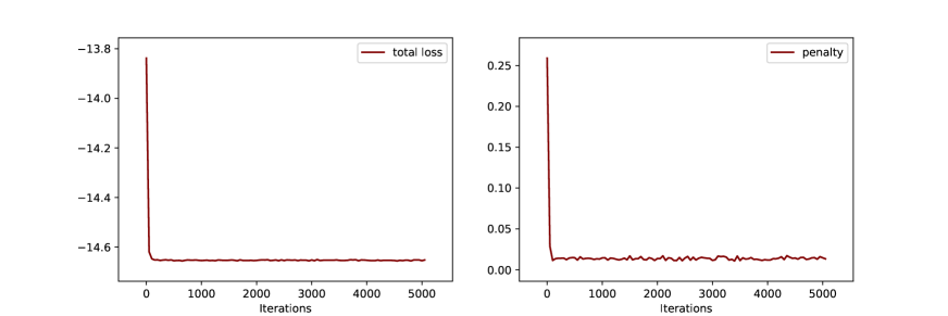
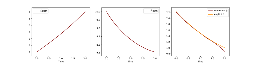
Figure 2: Results of the contract theory experiment where we have interactions through variance of the states and where we used the generalized penalty method. Top: total loss including the penalty cost (left), penalty cost (right), bottom: the paths of $\bar{X}$ (left) and $\bar{Y}$ (middle), and the comparison of the explicit effort level to the mean of the effort levels found by using the generalized penalty method (right). We see that the penalty cost is converging to levels close to $0$. It is also seen that the numerical approach is very good at mimicking the explicit results when the generalized numerical approach is used.

5.1.2 Experiment 2: interactions through the mean of the states

Second, we look at a case where the interactions among agents are through the mean of the states. In other words, we take $\beta_{2}=\gamma=0$. In this case, we expect the optimal effort of an agent is given as

$$\hat{\alpha}_{t}=\dfrac{e^{(a+\beta_{1})(T-t)}}{k}.$$ (5.7)

Again we test both numerical approaches (the one for the special case introduced in Section 4.2.2 and the generalized penalty method) against the explicit solutions and the results can be seen in Figures 3 and 4, respectively. Similar to the results of Experiment 1, we see that both methods are good at mimicking the explicit results and the penalty cost converges to the levels around $0$. Different than Experiment 1 (and Experiment 3 introduced below), in the generalized penalty method function approximator for $\xi$ is implemented with a recurrent neural network to allow it to be implemented as a function of the whole path of $\boldsymbol{X}$.

$T$	$\Delta t$	$\mu_{0}$	$\sigma$	$k$	$a$	$\beta_{1}$	$\beta_{2}$	$\gamma$
$2.0$	$0.02$	$\delta_{1}$	$1.0$	$1.0$	$0.4$	$0.25$	$0.0$	$0.0$

Table 2: Parameters used in experiment 2.

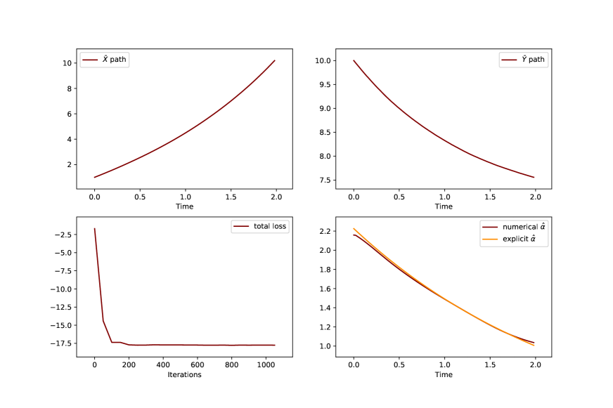
Figure 3: Results of the contract theory experiment where we have interactions through the mean of the state and where we use the algorithm proposed for the special case in Section 4.2.2. Top: the paths of $\bar{X}$ (left) and $\bar{Y}$ (right), bottom: total loss (left) and the comparison of the explicit effort level to the mean of the effort levels found by using the special numerical approach presented in Section 4.2.2 (right). It is seen that the special numerical approach is very good at mimicking the explicit results.

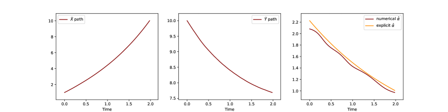
Figure 4: Results of the contract theory experiment where we have interactions through the mean of the states and where we used the generalized penalty method where $\xi$ is implemented as a recurrent neural network. Top: total loss including the penalty cost (left), penalty cost (right), bottom: the paths of $\bar{X}$ (left) and $\bar{Y}$ (middle), and the comparison of the explicit effort level to the mean of the effort levels found by using the generalized penalty method (right). We see that the penalty cost is converging to levels close to $0$. It is also seen that the numerical approach is good at mimicking the explicit results when the generalized numerical approach is used.

5.1.3 Experiment 3: interactions through the mean of the controls

In this section, in order to show the applicability of our numerical approach to extended MFGs, we look at a case where the interactions among agents are through the mean of the controls. In other words, we take $\beta_{1}=\gamma=0$. In this case, we expect the optimal effort of an agent is given as

$$\hat{\alpha}_{t}=(1+\beta_{2})\dfrac{e^{\alpha(T-t)}}{k}.$$ (5.8)

$T$	$\Delta t$	$\mu_{0}$	$\sigma$	$k$	$a$	$\beta_{1}$	$\beta_{2}$	$\gamma$
$2.0$	$0.02$	$\delta_{1}$	$1.0$	$1.0$	$0.4$	$0.0$	$0.5$	$0.0$

Table 3: Parameters used in experiment 3.

As we did in the experiments 1 and 2, we test both numerical approaches (the one for the special case introduced in Section 4.2.2 and the generalized penalty method) against the explicit solutions and the results can be seen in Figures 5 and 6, respectively. We see that in both algorithms, the numerical solutions are very good at mimicking the explicit solutions even when we have extended mean field games setup.

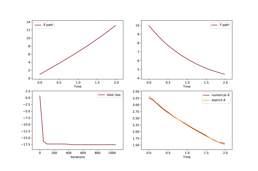
Figure 5: Results of the contract theory experiment where we have interactions through mean of the controls and where we use the algorithm proposed for the special case in Section 4.2.2. Top: the paths of $\bar{X}$ (left) and $\bar{Y}$ (right), bottom: total loss (left) and the comparison of the explicit effort level to the mean of the effort levels found by using the special numerical approach presented in Section 4.2.2 (right). It is seen that the special numerical approach is very good at mimicking the explicit results.

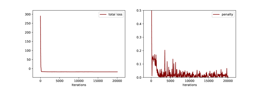
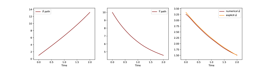
Figure 6: Results of the contract theory experiment where we have interactions through the mean of the controls and where we used the generalized penalty method. Top: total loss including the penalty cost (left), penalty cost (right), bottom: the paths of $\bar{X}$ (left) and $\bar{Y}$ (middle), and the comparison of the explicit effort level to the mean of the effort levels found by using the generalized penalty method (right). We see that the penalty cost is converging to levels close to $0$. It is also seen that the numerical approach is very good at mimicking the explicit results when the generalized numerical approach is used.

5.2 Systemic risk model under the influence of a principal

In this section, we focus on the systemic risk model that is analyzed in  [14, Ch. 3] and extend it by adding a regulator (i.e., principal). This model is introduced for modeling the borrowing and lending between banks. The state of the agents i.e., the banks is the logarithm of their cash reserve and the state of the representative agent at time $t$ is denoted as $X_{t}$. The dynamics of the log-cash reserve is given as:

$$dX_{t}=\big{[}a(\bar{X}_{t}-X_{t})+\alpha_{t}\big{]}dt+dW_{t}\,,$$ (5.9)

where $W_{t}$ is the idiosyncratic noise and $a>0$. The control of the representative bank i.e., the lending and borrowing amounts at time $t$ is denoted with $\alpha_{t}$. The objective of the representative bank is given as

$$\inf_{\alpha}\ \mathbb{E}\Big{[}\int_{0}^{T}\big{[}\dfrac{\alpha_{t}^{2}}{2}-\lambda(t)\alpha_{t}(\bar{X}_{t}-X_{t})+\dfrac{\epsilon}{2}(\bar{X}_{t}-X_{t})^{2}\big{]}dt+\dfrac{c}{2}(\bar{X}_{T}-X_{T})^{2}\Big{]}\,,$$ (5.10)

where $\epsilon,c,\lambda>0$ are coefficients and $\bar{X}_{t}=\int_{\mathbb{R}}xd\mu_{t}(x)$. Here, $\epsilon$ and $c$ balance the individual bank’s behavior with the average behavior of the other banks. $\lambda$ weighs the contribution of the components and helps to determine the sign of the control i.e., whether to borrow or to lend. Here, the model is extended by adding a regulator and the regulator’s control is the $\boldsymbol{\lambda}$. Here, if the log cash reserve of the individual bank is smaller than the empirical mean, then the bank will want to borrow and choose $\alpha_{t}>0$, and vice versa. We should assume $\lambda(t)^{2}\leq\epsilon,\ \forall t\in[0,T]$ in order to guarantee the convexity of the running cost functions while analyzing the explicit solution.

The regulator’s aim is to keep the coefficient $\lambda(t)$ around the aimed level, $\lambda^{aim}(t)$, $\forall t\in[0,T]$; furthermore, they want to minimize the proportion of banks defaulted. Mathematically the regulator’s objective is written as follows:

$$\inf_{\boldsymbol{\lambda}}\ \int_{0}^{T}(\lambda(t)-\lambda^{aim}(t))^{2}dt+\gamma\mathbb{E}\Big{[}\mathbbm{1}_{X_{T}<D}\Big{]},$$ (5.11)

where $D<0$ is a constant that represents the critical liability threshold. Below this level the bank is considered in a state of default.

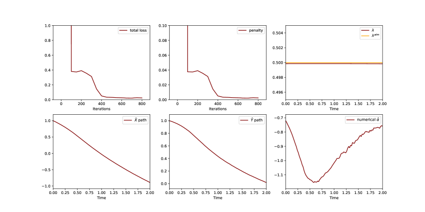
Figure 7: Results of the systemic risk experiment with the addition of a regulator that controls $\boldsymbol{\lambda}$. In this experiment, the regulator does not have a cost for the proportion of the banks defaulted, i.e., $\gamma=0$.) Top: total loss including the penalty cost (left), penalty cost (middle), comparison of the regulator’s aimed policy level and the numerical optimal policy level (right), Bottom: the paths of $\bar{X}$ (left) and $\bar{Y}$ (middle), the mean of the control of the banks found by using the generalized penalty method (right).

Following the model analysis given in Section 2.3, the Hamiltonian for the representative bank can be written as follows

$$H(t,X,\mu,z,\alpha;\lambda)=\left(a\left(\bar{X}-X\right)+\alpha\right)z+\dfrac{\alpha^{2}}{2}-\lambda\alpha\left(\bar{X}-X\right)+\dfrac{\epsilon}{2}\left(\bar{X}-X\right)^{2},$$ (5.12)

where $\bar{X}=\int_{\mathbb{R}}xd\mu(x)$. Then, the minimizer of the Hamiltonian is given as

$$\hat{\alpha}_{t}=\lambda(t)(\bar{X}_{t}-X_{t})-Z_{t}.$$ (5.13)

Finally, the system of FBSDE that characterize the mean field Nash equilibrium is given as

$$dX_{t} =\big{[}a(\bar{X}_{t}-X_{t})+\lambda(t)(\bar{X}_{t}-X_{t})-Z_{t}\big{]}dt+dW_{t}, X_{0}\sim\mu_{0}$$ (5.14)

$$dY_{t} =-\Big{[}\dfrac{(\lambda(t)(\bar{X}_{t}-X_{t})-Z_{t})^{2}}{2}-\lambda(t)(\lambda(t)(\bar{X}_{t}-X_{t})-Z_{t})(\bar{X}_{t}-X_{t})+$$

$$\hskip 170.71652pt\epsilon(\bar{X}_{t}-X_{t})^{2}\Big{]}dt+Z_{t}dW_{t},\quad Y_{T}=\dfrac{c}{2}(\bar{X}_{T}-X_{T})^{2}\,.$$

$T$	$\Delta t$	$\mu_{0}$	$a$	$c$	$\epsilon$	$\lambda^{\rm aim}$	$D$
$2.0$	$0.02$	$\delta_{1}$	$1.0$	$1.0$	$1.0$	$0.5$	$-0.001$

Table 4: Parameters used in the systemic risk experiment.

The model in this example does not fit in the special case form discussed in 4.2.2; therefore, we will be only presenting our results where we used the generalized penalty method. We first look at an example where the regulator does not have a cost for defaulting banks (i.e., $\gamma=0$). Here, we expect the regulator to choose $\hat{\lambda}(t)=\lambda(t)^{\rm aim}$. As it can be seen from Figure 7, our numerical approach is able to capture this phenomenon. Later, we also present results from an experiment where we include the cost related to the defaulted banks for the regulator (i.e., $\gamma\neq 0$). From Figure 8, we can see that the optimal policy of the regulator is different than the $\lambda(t)^{\rm aim}$ in order to decrease the proportion of banks defaulting.

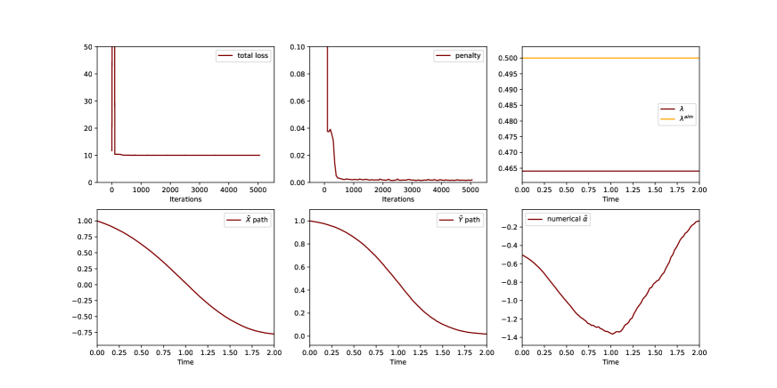
Figure 8: Results of the systemic risk experiment with the addition of a regulator that controls $\boldsymbol{\lambda}$. In this experiment, the regulator has a cost for the proportion of the banks defaulted. ($\gamma=10$) Top: total loss including the penalty cost (left), penalty cost (middle), comparison of the regulator’s aimed policy level and the numerical optimal policy level (right), Bottom: the paths of $\bar{X}$ (left) and $\bar{Y}$ (middle), the mean of the control of the banks found by using the generalized penalty method (right).

6 Conclusion

In this paper, we propose a numerical approach to solve Stackelberg MFG. In such problems, the principal aims to optimize her policy while taking into account the reaction of the strategic agents to this policy. This creates a bi-level problem where, at the population level, the agents solve a mean field Nash equilibrium given the policy and, at the upper level, the principal looks for the optimal policy. We first rewrite this problem as a single-level problem to solve it efficiently and introduce a numerical approach that uses neural networks and Monte Carlo simulation. On the theoretical side, we first show the convergence of the solution of the reformulated problem to the solution of the original problem. Second, we show the convergence of the solution of the parameterized problem to the solution of the reformulated problem to motivate our numerical approach. We also show that the numerical approach can be extended to more complex model forms where the principal has a contract theory type of problem with an additional $\mathcal{F}_{T}$-measurable incentive. Lastly, we show the effectiveness of the proposed numerical approach with two different examples.

References

• [1] Y. Achdou, F. Camilli, and I. Capuzzo-Dolcetta, Mean field games: numerical methods for the planning problem, SIAM Journal on Control and Optimization, 50 (2012), pp. 77–109.
• [2] Y. Achdou and I. Capuzzo-Dolcetta, Mean field games: numerical methods, SIAM Journal on Numerical Analysis, 48 (2010), pp. 1136–1162.
• [3] Y. Achdou, P. Cardaliaguet, F. Delarue, A. Porretta, F. Santambrogio, Y. Achdou, and M. Laurière, Mean field games and applications: Numerical aspects, Mean Field Games: Cetraro, Italy 2019, (2020), pp. 249–307.
• [4] A. Angiuli, C. V. Graves, H. Li, J.-F. Chassagneux, F. Delarue, and R. Carmona, Cemracs 2017: numerical probabilistic approach to mfg, ESAIM: Proceedings and Surveys, 65 (2019), pp. 84–113.
• [5] A. Aurell, R. Carmona, G. Dayanikli, and M. Laurière, Optimal incentives to mitigate epidemics: A stackelberg mean field game approach, SIAM Journal on Control and Optimization, 60 (2022), pp. S294–S322.
• [6] A. Bensoussan, M. Chau, Y. Lai, and S. C. P. Yam, Linear-quadratic mean field stackelberg games with state and control delays, SIAM Journal on Control and Optimization, 55 (2017), pp. 2748–2781.
• [7] A. Bensoussan, M. H. M. Chau, and S. C. P. Yam, Mean field Stackelberg games: aggregation of delayed instructions, SIAM J. Control Optim., 53 (2015), pp. 2237–2266.
• [8] A. Bensoussan, J. Frehse, P. Yam, et al., Mean field games and mean field type control theory, vol. 101, Springer, 2013.
• [9] L. M. Briceno-Arias, D. Kalise, and F. J. Silva, Proximal methods for stationary mean field games with local couplings, SIAM Journal on Control and Optimization, 56 (2018), pp. 801–836.
• [10] S. Campbell, Y. Chen, A. Shrivats, and S. Jaimungal, Deep learning for principal-agent mean field games, 2021.
• [11] E. Carlini and F. J. Silva, A fully discrete semi-lagrangian scheme for a first order mean field game problem, SIAM Journal on Numerical Analysis, 52 (2014), pp. 45–67.
• [12] R. Carmona and G. Dayanıklı, Mean field game model for an advertising competition in a duopoly, International Game Theory Review, 23 (2021), p. 2150024.
• [13] R. Carmona, G. Dayanıklı, and M. Laurière, Mean field models to regulate carbon emissions in electricity production, Dynamic Games and Applications, (2022).
• [14] R. Carmona and F. Delarue, Probabilistic Theory of Mean Field Games with Applications I: Mean Field FBSDEs, Control, and Games, Probability Theory and Stochastic Modelling, Springer International Publishing, 2018.
• [15]  , Probabilistic Theory of Mean Field Games with Applications II: Mean Field Games with Common Noise and Master Equations, Probability Theory and Stochastic Modelling, Springer International Publishing, 2018.
• [16] R. Carmona and M. Laurière, Convergence analysis of machine learning algorithms for the numerical solution of mean field control and games: II - the finite horizon case, Accepted in Annals of Applied Probability. arXiv preprint arXiv:1908.01613, (2021).
• [17] R. Carmona and P. Wang, Finite-state contract theory with a principal and a field of agents, Management Science, (2020), p. First on line.
• [18] J.-F. Chassagneux, D. Crisan, and F. Delarue, Numerical method for fbsdes of mckean–vlasov type, The Annals of Applied Probability, 29 (2019), pp. 1640–1684.
• [19] J. Cvitanić, D. Possamaï, and N. Touzi, Dynamic programming approach to principal–agent problems, Finance and Stochastics, 22 (2018), pp. 1–37.
• [20] G. Cybenko, Approximation by superpositions of a sigmoidal function, Mathematics of control, signals and systems, 2 (1989), pp. 303–314.
• [21] B. Djehiche and P. Helgesson, The principal-agent problem; a stochastic maximum principle approach. preprint, 2014.
• [22] R. Elie, T. Mastrolia, and D. Possamaï, A tale of a principal and many, many agents, Mathematics of Operations Research, 44 (2019), pp. 440–467.
• [23] R. Elie, T. Mastrolia, and D. Possamaï, A tale of a principal and many, many agents, Mathematics of Operations Research, 44 (2019), pp. 440–467.
• [24] J.-P. Fouque and Z. Zhang, Deep learning methods for mean field control problems with delay, Frontiers in Applied Mathematics and Statistics, 6 (2020), p. 11.
• [25] D. Gomes, J. Gutiérrez, and M. Laurière, Machine learning architectures for price formation models, arXiv preprint arXiv:2204.03968, (2022).
• [26] J. Han and R. Hu, Recurrent neural networks for stochastic control problems with delay, Mathematics of Control, Signals, and Systems, 33 (2021), pp. 775–795.
• [27] B. Holmstrom and P. Milgrom, Aggregation and linearity in the provision of intertemporal incentives, Econometrica: Journal of the Econometric Society, (1987), pp. 303–328.
• [28] K. Hornik, Approximation capabilities of multilayer feedforward networks, Neural networks, 4 (1991), pp. 251–257.
• [29] K. Hornik, M. Stinchcombe, and H. White, Universal approximation of an unknown mapping and its derivatives using multilayer feedforward networks, Neural networks, 3 (1990), pp. 551–560.
• [30] K. Hu, Z. Ren, and J. Yang, Principal-agent problem with multiple principals, Stochastics, (2022), pp. 1–28.
• [31] M. Huang, R. P. Malhamé, P. E. Caines, et al., Large population stochastic dynamic games: closed-loop McKean-Vlasov systems and the Nash certainty equivalence principle, Communications in Information & Systems, 6 (2006), pp. 221–252.
• [32] E. Hubert, T. Mastrolia, D. Possamaï, and X. Warin, Incentives, lockdown, and testing: from Thucydides’s analysis to the COVID-19 pandemic. preprint, 2020.
• [33] J.-M. Lasry and P.-L. Lions, Jeux à champ moyen. I–le cas stationnaire, Comptes Rendus Mathématique, 343 (2006), pp. 619–625.
• [34]  , Jeux à champ moyen. II–horizon fini et contrôle optimal, Comptes Rendus Mathématique, 343 (2006), pp. 679–684.
• [35] Y. Lin, X. Jiang, and W. Zhang, An open-loop stackelberg strategy for the linear quadratic mean-field stochastic differential game, IEEE Transactions on Automatic Control, 64 (2018), pp. 97–110.
• [36] J. Moon and T. Başar, Linear quadratic mean field stackelberg differential games, Automatica, 97 (2018), pp. 200–213.
• [37] A. Pinkus, Approximation theory of the mlp model in neural networks, Acta numerica, 8 (1999), pp. 143–195.
• [38] R. Salhab, R. Malhamé, and J. L. Ny, A dynamic collective choice model with an advertiser, 2016 IEEE 55th Conference on Decision and Control (CDC), (2016), pp. 6098–6104.
• [39] Y. Sannikov, A Continuous- Time Version of the Principal: Agent Problem, The Review of Economic Studies, 75 (2008), pp. 957–984.
• [40] Y. Sannikov, Contracts: The Theory of Dynamic Principal–Agent Relationships and the Continuous-Time Approach, vol. 1 of Econometric Society Monographs, Cambridge University Press, 2013, p. 89–124.