Tackling Shortcut Learning in Deep Neural Networks: An Iterative Approach with Interpretable Models

Abstract

We use concept-based interpretable models to mitigate shortcut learning. Existing methods lack interpretability. Beginning with a Blackbox, we iteratively carve out a mixture of interpretable experts (MoIE) and a residual network. Each expert explains a subset of data using First Order Logic (FOL). While explaining a sample, the FOL from biased BB-derived MoIE detects the shortcut effectively. Finetuning the BB with Metadata Normalization (MDN) eliminates the shortcut. The FOLs from the finetuned-BB-derived MoIE verify the elimination of the shortcut. Our experiments show that MoIE does not hurt the accuracy of the original BB and eliminates shortcuts effectively.

1 Introduction

Shortcuts pose a significant challenge to the generalizability of deep neural networks, denoted as Blackbox (BB), in real-world scenarios (Geirhos et al., 2020; Kaushik et al., 2019). Referred to as spurious correlations, shortcuts indicate statistical associations between class labels and coincidental features that lack a meaningful causal connection. When trained on a dataset with shortcuts, a BB performs poorly when applied to test data without these shortcuts. This restricted generalization capability engenders a crucial concern, particularly in critical applications e.g., medical diagnosis (Bissoto et al., 2020).

Various methods e.g., invariant learning (Arjovsky et al., 2020), correlation alignment (Sun & Saenko, 2016), variance penalty (Krueger et al., 2021), gradient alignment (Shi et al., 2021), instance reweighting (Sagawa et al., 2019; Liu et al., 2021), and data augmentation (Xu et al., 2020; Yao et al., 2022) have been employed to address the issue of shortcuts in Empirical Risk Minimization (ERM) models. However, they lack interpretability in 3 pivotal areas: 1) pinpointing the precise shortcut that the BB is aimed at, 2) clarifying the mechanism through which a particular shortcut is eradicated from the BB’s representation, and 3) establishing a dependable technique to verify the elimination of the shortcut. The application of LIME (Ribeiro et al., 2016) and proxy-based interpretable models (Rosenzweig et al., 2021) have been investigated to detect shortcuts in Explainable AI. However, they function within the pixel space rather than the human interpretable concept space (Kim et al., 2017) and fail to address the issue of shortcut learning. This paper addresses this gap utilizing concept-based models.

Concept-based interpretable by design models (Koh et al., 2020; Zarlenga et al., 2022) use 1) a concept classifier to detect the presence/absence of concepts in an image, 2) an interpretable function (e.g., linear regression or rule-based) to map the concepts to the final output. However, these approaches utilize a single interpretable model to explain the whole dataset failing to encompass the diverse instance-specific explanations and exhibiting inferior performance than their BB counterparts.

Our contributions. This paper proposes a novel method using the concept-based interpretable model to eliminate the shortcut learning problem. First we carve out a mixture of interpretable models and a residual network from a given BB. We hypothesize that a BB encodes multiple interpretable models, each pertinent to a unique data subset. As each interpretable model specializes over a subset of data, we refer to them as expert. Our design routes the samples through the interpretable models to explain them with FOL. The remaining samples are routed through a residual network. On the residual, we repeat the method until all the experts explain the desired proportion of data. Next, we employ MDN (Lu et al., 2021), a batch-level operation, to mitigate the impact of extraneous variables (metadata) on feature distributions. This approach effectively eliminates metadata effects during the training process. Specifically, we deploy a 3-step procedure to mitigate the shortcuts:

• The FOLs from biased BB detect the presence of the shortcut,

• Assuming the detected shortcut as metadata, we use MDN layers to eliminate the shortcut by finetuning the BB,

• The FOLs from the fine-tuned BB verify the elimination of the shortcut.

2 Method

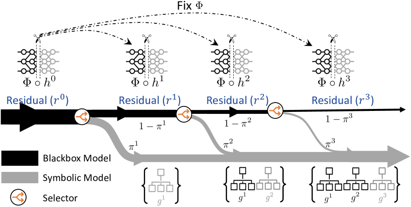
Figure 1: Schematic view of our method. Note that $f^{k}(.)=h^{k}(\Phi(.))$. At iteration $k$, the selector routes each sample either towards the expert $g^{k}$ with probability $\pi^{k}(.)$ or the residual $r^{k}=f^{k-1}-g^{k}$ with probability $1-\pi^{k}(.)$. $g^{k}$ generates FOLs to explain the samples it covers. Note $\Phi$ is fixed across iterations.

Notation: Assume $f^{0}:\mathcal{X}\rightarrow\mathcal{Y}$ is a BB, on a dataset $\mathcal{X}\times\mathcal{Y}\times\mathcal{C}$, with $\mathcal{X}$, $\mathcal{Y}$, and $\mathcal{C}$ being the images, classes, and concepts, respectively; $f^{0}=h^{0}\circ\Phi$, where $\Phi$ and $h^{0}$ is the feature extractor and the classifier respectively. $f^{0}$ predicts $\mathcal{Y}$ from the input $\mathcal{X}$. Given a learnable projection (Ghosh et al., 2023), $t:\Phi\rightarrow\mathcal{C}$, our method learns three functions: (1) a set of selectors ($\pi:\mathcal{C}\rightarrow\{0,1\}$) routing samples to an interpretable model or residual, (2) a set of interpretable models ($g:\mathcal{C}\rightarrow\mathcal{Y}$), and (3) the residuals. The interpretable models are called “experts” since they specialize in a distinct subset of data defined by that iteration’s coverage $\tau$ as shown in SelectiveNet (Rabanser et al., 2022). Fig. 1 illustrates our method.

2.1 Distilling BB to the mixture of interpretable models

The selectors: As the first step of our method, the selector $\pi^{k}$ routes the $j^{th}$ sample through the interpretable model $g^{k}$ or residual $r^{k}$ with probability $\displaystyle\pi^{k}(\boldsymbol{c_{j}})$ and $\displaystyle 1-\pi^{k}(\boldsymbol{c_{j}})$ respectively, where $k$ $\in[0,K]$, with $K$ being the number of iterations. We define the empirical coverage of the $\displaystyle k^{th}$ iteration as $\vspace{-0.08pt}\zeta(\pi^{k})=\frac{1}{m}\sum_{j=1}^{m}\pi^{k}(\boldsymbol{c_{j}})\vspace{-0.081pt}$, the empirical mean of the samples selected by the selector for the associated interpretable model $\displaystyle g^{k}$, with $\displaystyle m$ being the total number of samples in the training set. Thus, the entire selective risk is: $\mathcal{R}^{k}(\displaystyle\pi^{k},\displaystyle g^{k})=\frac{\frac{1}{m}\sum_{j=1}^{m}\mathcal{L}_{(g^{k},\pi^{k})}^{k}\big{(}\boldsymbol{x_{j}},\boldsymbol{c_{j}}\big{)}}{\zeta(\pi^{k})},$ where $\mathcal{L}_{(g^{k},\pi^{k})}^{k}$ is the optimization loss used to learn $\displaystyle g^{k}$ and $\displaystyle\pi^{k}$ together, discussed in the next section. For a given coverage of $\displaystyle\tau^{k}\in(0,1]$, we solve the following optimization problem:

$$\theta_{s^{k}}^{*},\theta_{g^{k}}^{*}= \operatorname*{arg\,min}_{\theta_{s^{k}},\theta_{g^{k}}}\mathcal{R}^{k}\Big{(}\pi^{k}(.;\theta_{s^{k}}),\displaystyle g^{k}(.;\theta_{g^{k}})\Big{)}$$

$$\text{s.t.}~{}~{}~{}\zeta\big{(}\pi^{k}(.;\theta_{s^{k}})\big{)}\geq\tau^{k},$$ (1)

where $\theta_{s^{k}}^{*},\theta_{g^{k}}^{*}$ are the optimal parameters at iteration $k$ for the selector $\pi^{k}$ and the interpretable model $g^{k}$ respectively. In this work, $\pi$s’ of different iterations are neural networks with sigmoid activation. At inference time, the selector routes the $j^{th}$ sample with concept vector $\boldsymbol{c_{j}}$ to $\displaystyle g^{k}$ if and only if $\pi^{k}(\boldsymbol{c}_{j})\geq 0.5$ for $k\in[0,K]$.

Algorithm 1 Applying MoIE to eliminate shortcuts

1:  Input: $\mathcal{D}$ = {$x_{j}$, $c_{j}$, $y_{j}$}${}_{j=1}^{n}$; biased BB $f^{0}=h^{0}(\Phi(.))$; The total iterations K; Coverages $\tau_{1},\dots,\tau_{K}$. Freeze $\Phi$.

2:  Using (Yuksekgonul et al., 2022) learn the projection $t$ to predict the concept value.

3:  Detection step. Learn the experts in MoIE $\{g\}_{k=1}^{K}$ and extract the FOLs. The FOL contains shortcuts.

4:  Elimination step. Consider the detected shortcut concept in the “Detection” step as metadata and finetune BB ($f^{0}$) with MDN (Lu et al., 2021) to remove the role of that shortcut.

5:  Retrain $t$ with $\Phi$ of finetuned BB to get the concepts.

6:  Verification step. Learn MoIE $\{g\}_{k=1}^{K}$ again from retrained $t$ and recompute the FOLs. The final FOLs do not contain spurious concepts as they have been eliminated in the “Elimination step”.

Table 1: Datasets and BlackBoxes.

DATASET	BB	# EXPERTS
CUB-200 (Wah et al., 2011)	RESNET101 (He et al., 2016)	6
CUB-200 (Wah et al., 2011)	VIT (Wang et al., 2021)	6
AWA2 (Xian et al., 2018)	RESNET101 (He et al., 2016)	4
AWA2 (Xian et al., 2018)	VIT (Wang et al., 2021)	6
HAM1000 (Tschandl et al., 2018)	INCEPTION (Szegedy et al., 2015)	6
SIIM-ISIC (Rotemberg et al., 2021)	INCEPTION (Szegedy et al., 2015)	6
EFFUSION IN MIMIC-CXR (Johnson et al., )	DENSENET121 (Huang et al., 2017)	3

The experts: For iteration $k$, the loss $\mathcal{L}_{(g^{k},\pi^{k})}^{k}$ distills the expert $g^{k}$ from $f^{k-1}$, BB of the previous iteration:

where the term $\pi^{k}(\boldsymbol{c_{j}})\prod_{i=1}^{k-1}\big{(}1-\pi^{i}(\boldsymbol{c_{j}})\big{)}$ denotes the probability of the sample going through the residuals for all the previous iterations from $1$ through $k-1$ (i.e., $\prod_{i=1}^{k-1}\big{(}1-\pi^{i}(\boldsymbol{c_{j}})\big{)}$) times the probability of going through the interpretable model at iteration $k$ (i.e., $\pi^{k}(\boldsymbol{c_{j}})$). At iteration $k$, $\pi^{1},\dots\pi^{k-1}$ are not trainable.

Table 2: MoIE does not hurt the performance of the original BB. We provide AUROC and accuracy for medical imaging (e.g., HAM10000, ISIC, and Effusion) and vision (e.g., CUB-200 and Awa2) datasets, respectively, over 5 random seeds. For MoIE, we also report the “Coverage”. We only report the performance of the convolutional CEM (Zarlenga et al., 2022), leaving the construction of VIT-based CEM as future work. As HAM10000 and ISIC have no concept annotation, interpretable-by-design models can not be constructed.

MODEL	DATASET
	CUB-200 (RESNET101)	CUB-200 (VIT)	AWA2 (RESNET101)	AWA2 (VIT)	HAM10000	SIIM-ISIC	EFFUSION
BLACKBOX	0.88	0.92	0.89	0.99	0.96	0.85	0.91
INTERPRETABLE-BY-DESIGN
CEM (Zarlenga et al., 2022)	0.77 $\pm$ 0.002	-	0.88 $\pm$ 0.005	-	NA	NA	0.76 $\pm$ 0.002
CBM (Sequential) (Koh et al., 2020)	0.65 $\pm$ 0.003	0.86 $\pm$ 0.002	0.88 $\pm$ 0.003	0.94 $\pm$ 0.002	NA	NA	0.79 $\pm$ 0.005
CBM + E-LEN (Koh et al., 2020; Barbiero et al., 2022)	0.71 $\pm$ 0.003	0.88 $\pm$ 0.002	0.86 $\pm$ 0.003	0.93 $\pm$ 0.002	NA	NA	0.79 $\pm$ 0.002
POSTHOC
PCBM (Yuksekgonul et al., 2022)	0.76 $\pm$ 0.001	0.85 $\pm$ 0.002	0.82 $\pm$ 0.002	0.94 $\pm$ 0.001	0.93 $\pm$ 0.001	0.71 $\pm$ 0.012	0.81 $\pm$ 0.017
PCBM-h (Yuksekgonul et al., 2022)	0.85 $\pm$ 0.001	0.91 $\pm$ 0.001	0.87 $\pm$ 0.002	0.98 $\pm$ 0.001	0.95 $\pm$ 0.001	0.79 $\pm$ 0.056	0.87 $\pm$ 0.072
PCBM + E-LEN (Yuksekgonul et al., 2022; Barbiero et al., 2022)	0.80 $\pm$ 0.003	0.89 $\pm$ 0.002	0.85 $\pm$ 0.002	0.96 $\pm$ 0.001	0.94 $\pm$ 0.021	0.73 $\pm$ 0.011	0.81 $\pm$ 0.014
PCBM-h + E-LEN (Yuksekgonul et al., 2022; Barbiero et al., 2022)	0.85 $\pm$ 0.003	0.91 $\pm$ 0.002	0.88 $\pm$ 0.002	0.98 $\pm$ 0.002	0.95 $\pm$ 0.032	0.82 $\pm$ 0.056	0.87 $\pm$ 0.032
OURS
MoIE (COVERAGE)	0.86 $\pm$ 0.001 (0.9)	0.91 $\pm$ 0.001 (0.95)	0.87 $\pm$ 0.002 (0.91)	0.97 $\pm$ 0.004 (0.94)	0.95 $\pm$ 0.001 (0.9)	0.84 $\pm$ 0.001 (0.94)	0.87 $\pm$ 0.001 (0.98)
MoIE + RESIDUAL	0.84 $\pm$ 0.001	0.90 $\pm$ 0.001	0.86 $\pm$ 0.002	0.94 $\pm$ 0.004	0.92 $\pm$ 0.00	0.82 $\pm$ 0.01	0.86 $\pm$ 0.00

Table 3: Performance of various shortcut elimination methods on Waterbirds dataset.

Method	Avg Acc.	Worst Acc.
ERM (Wah et al., 2011)	97.0 $\pm$ 0.2%	63.7 $\pm$ 1.9%
ERM+aug (Wah et al., 2011)	87.4 $\pm$ 0.5%	76.4 $\pm$ 2.0%
UW (Xian et al., 2018)	96.3.0 $\pm$ 0.3%	76.2 $\pm$ 1.4%
IRM (Arjovsky et al., 2020)	87.5 $\pm$ 0.7%	75.6 $\pm$ 3.1%
IB-IRM (Ahuja et al., 2022)	88.5 $\pm$ 0.9%	76.5 $\pm$ 1.2%
V-REx (Krueger et al., 2021)	88.0 $\pm$ 1.4%	73.6 $\pm$ 0.2%
CORAL (Sun & Saenko, 2016)	90.3 $\pm$ 1.1%	79.8 $\pm$ 1.8%
Fish (Shi et al., 2021)	85.6 $\pm$ 0.4%	64.0 $\pm$ 0.3%
GroupDRO (Sagawa et al., 2019)	91.8 $\pm$ 0.3%	90.6 $\pm$ 1.1%
JTT (Liu et al., 2021)	93.3 $\pm$ 0.3%	86.7 $\pm$ 1.5%
DM-ADA (Xu et al., 2020)	76.4 $\pm$ 0.3%	53.0 $\pm$ 1.3%
LISA (Yao et al., 2022)	91.8 $\pm$ 0.3%	88.5 $\pm$ 0.8%
BB w MDN (ours)	95.01 $\pm$ 0.5%	94.4 $\pm$ 0.5%
MoIE from BB w MDN (ours) (COVERAGE)	91.0 $\pm$ 0.5% (0.91)	93.7 $\pm$ 0.4% (0.87)
MoIE+R from BB w MDN (ours)	90.2 $\pm$ 0.5%	92.1 $\pm$ 0.4%

The Residuals: The last step is to repeat with the residual $r^{k}$, as $\displaystyle r^{k}(\boldsymbol{x_{j}},\boldsymbol{c_{j}})=f^{k-1}(\boldsymbol{x_{j}})-g^{k}(\boldsymbol{c_{j}})$. We fix $\Phi$ and optimize the following loss to update $h^{k}$ to specialize on those samples not covered by $g^{k}$, effectively creating a new BB $f^{k}$ for the next iteration $(k+1)$:

$$\mathcal{L}_{f}^{k}(\boldsymbol{x_{j}},\boldsymbol{c_{j}})=\underbrace{\vrule width=0.0pt,height=0.0pt,depth=11.19443pt\ell\big{(}r^{k}(\boldsymbol{x_{j}},\boldsymbol{c_{j}}),f^{k}(\boldsymbol{x_{j}})\big{)}}_{\begin{subarray}{c}\text{trainable component}\\ \text{for iteration $k$}\end{subarray}}\underbrace{\vrule width=0.0pt,height=0.0pt,depth=11.19443pt\prod_{i=1}^{k}\big{(}1-\pi^{i}(\boldsymbol{c_{j}})\big{)}}_{\begin{subarray}{c}\text{non-trainable component}\\ \text{for iteration $k$}\end{subarray}}$$ (3)

We refer to all the experts as the Mixture of Interpretable Experts (MoIE). We denote the experts, including the final residual, as MoIE+R. Each expert in MoIE constructs sample-specific FOLs using the optimization strategy in SelectiveNet (Geifman & El-Yaniv, 2019).

2.2 Applying to mitigate shortcuts

Algorithm 1 illustrates a 3-step procedure to eliminate shortcuts. The BB, trained on a dataset with shortcuts, latches on the spurious concepts to classify the labels. Detection. The FOLs from the biased BB-derived MoIE, capture the spurious concepts. Elimination. Assuming the spurious concepts as metadata, we minimize the effect of shortcuts from the representation of the BB using MDN (Lu et al., 2021) layers between two successive layers of the convolutional backbone to fine-tune the biased BB. MDN is a regression-based normalization technique to mitigate metadata effects and improve model robustness. Verfitication. Finally, we distill the MoIE from the new robust BB and generate the FOLs. The FOLs validate if the BB still uses spurious concepts for prediction.

3 Experiments

We perform experiments to show that MoIE does not compromise the accuracy of the original BB across various datasets and architectures and eliminates shortcuts using the Waterbirds dataset (Sagawa et al., 2019). As a stopping criterion, we repeat our method until MoIE covers at least 90% of samples. Furthermore, we only include concepts as input to $g$ if their validation accuracy or AUROC exceeds a certain threshold (in all of our experiments, we fix 0.7 or 70% as the threshold of validation auroc or accuracy). Refer to Table 1 for the datasets and BBs’ experimented with. For ResNets, Inception, and DenseNet121, we flatten the feature maps from the last convolutional block to extract the concepts. For VITs, we use the image embeddings from the transformer encoder to perform the same. We use SIIM-ISIC as a real-world transfer learning setting, with the BB trained on HAM10000 and evaluated on a subset of the SIIM-ISIC Melanoma Classification dataset (Yuksekgonul et al., 2022). Section A.2 and Section A.3 expand on the datasets and hyperparameters. Furthermore, we utilize E-LEN, i.e., a Logic Explainable Network (Ciravegna et al., 2023) implemented with an Entropy Layer as first layer (Barbiero et al., 2022) as the interpretable symbolic model $g$ to construct FOL explanations of a given prediction. With ResNet50 as the BB for shortcut detection, we use MDN layers between convolution blocks.

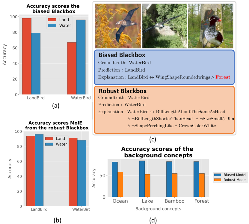
Figure 2: MoIE fixes shortcuts. Performance of (a) the biased BB and (b) final MoIE extracted from the robust BB. (c) Examples of samples (top-row) and FOLs extracted from the biased (middle-row) and robust BB (bottom-row). (d) Accuracies of the spurious concepts extracted from the biased vs. the robust BB.

Baselines: To show the efficacy of our method compared to other concept-based models, we compare our methods to two concept-based baselines – 1) interpretable-by-design and 2) posthoc. They consist of two parts: a) a concept predictor $\Phi:\mathcal{X}\rightarrow\mathcal{C}$, predicting concepts from images; and b) a label predictor $g:\mathcal{C}\rightarrow\mathcal{Y}$, predicting labels from the concepts. The end-to-end CEMs and sequential CBMs serve as interpretable-by-design baselines. Similarly, PCBM and PCBM-h serve as post hoc baselines. Convolution-based $\Phi$ includes all layers till the last convolution block. VIT-based $\Phi$ consists of the transformer encoder block. The standard CBM and PCBM models do not show how the concepts are composed to make the label prediction. So, we create CBM + E-LEN, PCBM + E-LEN, and PCBM-h + E-LEN by using the identical $g$ of MOIE (shown in Section A.3), as a replacement for the standard classifiers of CBM and PCBM. We train the $\Phi$ and $g$ in these new baselines to sequentially generate FOLs (Barbiero et al., 2022). Due to the unavailability of concept annotations, we extract the concepts from the Derm7pt dataset (Kawahara et al., 2018) using the pre-trained embeddings of the BB (Yuksekgonul et al., 2022) for HAM10000. Thus, we do not have interpretable-by-design baselines for HAM10000 and ISIC.

For shortcut-based methods, we compare our method with Empirical Risk Minimization (ERM) with and without data augmentations; Up- weighting (UW), which weights the instances of minority groups; Invariant Learning algorithms: IRM (Arjovsky et al., 2020), IB-IRM (Ahuja et al., 2022); Domain generalization/adaptation methods: V-REx (Krueger et al., 2021), CORAL (Sun & Saenko, 2016), and Fish (Shi et al., 2021); Instance reweighting methods: GroupDRO (Sagawa et al., 2020), JTT (Liu et al., 2021); Data augmentation methods: DM-ADA (Xu et al., 2020), LISA (Yao et al., 2022).

4 Results

MoIE does not compromise the performance of the original BB. As MoIE uses multiple experts covering different subsets of data compared to the single one by the baselines, MoIE outperforms the baselines for most of the datasets, shown in Table 2. Awa2 comprises rich concept annotation for zero-shot learning, resulting in better performance for the interpretable-by-design baselines. Section A.4 illustrates that MoIE captures a diverse set of concepts qualitatively. Figure 8 shows that later iterations of MoIE cover the “harder” examples.

Eliminating shortcuts. Table 3 demonstrates the efficacy of MoIE in eliminating the shortcuts than the other shortcut removal method by achieving high worst-case accuracy. First, the BB’s accuracy differs for land-based versus aquatic subsets of the bird species, as shown in Figure 2a. The Waterbird on the water is more accurate than on land (96% vs. 67% in the red bar). In the interpretable “Detection” stage, the FOLs from the biased BB-derived MoIE detect the spurious background concept forest for a waterbird, misclassified as a landbird in Figure 2c (top row). In the “Elimination” stage, the fine-tuned BB with MDN layers removes the specific background from the BB’s representation ($\Phi$). Next, we train $t$, using $\Phi$ of the finetuned BB, and compare the accuracy of the spurious concepts with the biased BB in Figure 2d. The validation accuracy of all the spurious concepts retrieved from the finetuned BB falls well short of the predefined threshold of 70% compared to the biased BB. Finally, we distill the MoIE from the robust BB. Figure 2b illustrates similar accuracies of MoIE for Waterbirds on water vs. Waterbirds on land (89% - 91%). As the shortcut concepts are removed successfully, MoIE outperforms the other shortcut removal methods in worst group accuracy in Table 3 (the last 2 rows). In the interpretable “Verification” stage, the FOL from the robust BB does not include any background concepts ( 2c, bottom row).

5 Conclusion

This paper proposes a novel method to iteratively extract a mixture of interpretable models from a flexible BB to eliminate shortcuts. We aim to leverage MoIE to eliminate shortcuts with varying complexities in the future.

Appendix A Appendix

A.1 Code

Refer to the url https://github.com/AI09-guy/ICML-Submission/ for the code.

Neuro-symbolic AI is an area of study that encompasses deep neural networks with symbolic approaches to computing and AI to complement the strengths and weaknesses of each, resulting in a robust AI capable of reasoning and cognitive modeling (Belle, 2020). Neuro-symbolic systems are hybrid models that leverage the robustness of connectionist methods and the soundness of symbolic reasoning to effectively integrate learning and reasoning (Garcez et al., 2015; Besold et al., 2017).

A.2 Dataset

CUB-200

The Caltech-UCSD Birds-200-2011 ((Wah et al., 2011)) is a fine-grained classification dataset comprising 11788 images and 312 noisy visual concepts. The aim is to classify the correct bird species from 200 possible classes. We adopted the strategy discussed in (Barbiero et al., 2022) to extract 108 denoised visual concepts. Also, we utilize training/validation splits shared in (Barbiero et al., 2022). Finally, we use the state-of-the-art classification models Resnet-101 ((He et al., 2016)) and Vision-Transformer (VIT) ((Wang et al., 2021)) as the blackboxes $f^{0}$.

Animals with attributes2 (Awa2)

AwA2 dataset (Xian et al., 2018) consists of 37322 images of a total of 50 animal classes with 85 numeric attributes. We use the state-of-the-art classification models Resnet-101 ((He et al., 2016)) and Vision-Transformer (VIT) ((Wang et al., 2021)) as the blackboxes $f^{0}$.

HAM10000

HAM10000 ((Tschandl et al., 2018)) is a classification dataset aiming to classify a skin lesion as benign or malignant. Following (Daneshjou et al., 2021), we use Inception (Szegedy et al., 2015) model, trained on this dataset as the blackbox $f^{0}$. We follow the strategy in (Lucieri et al., 2020) to extract the eight concepts from the Derm7pt ((Kawahara et al., 2018)) dataset.

SIIM-ISIC

To test a real-world transfer learning use case, we evaluate the model trained on HAM10000 on a subset of the SIIM-ISIC(Rotemberg et al., 2021)) Melanoma Classification dataset. We use the same concepts described in the HAM10000 dataset.

MIMIC-CXR

We use 220,763 frontal images from the MIMIC-CXR dataset (Johnson et al., ) aiming to classify effusion. We obtain the anatomical and observation concepts from the RadGraph annotations in RadGraph’s inference dataset ((Jain et al., 2021)), automatically generated by DYGIE++ ((Wadden et al., 2019)). We use the test-train-validation splits from (Yu et al., 2022) and Densenet121 (Huang et al., 2017) as the blackbox $f^{0}$.

Waterbirds

(Sagawa et al., 2019) creates the Waterbirds dataset by using forest and bamboo as the spurious land concepts of the Places dataset for landbirds of the CUB-200 dataset. We do the same by using oceans and lakes as the spurious water concepts for waterbirds. We utilize ResNet50 as the Blackbox $f^{0}$ to identify each bird as a Waterbird or a Landbird.

A.3 Architectural details of symbolic experts and hyperparameters

Table 4 demonstrates different settings to train the Blackbox of CUB-200, Awa2 and MIMIC-CXR respectively. For the VIT-based backbone, we used the same hyperparameter setting used in the state-of-the-art Vit-B_16 variant in (Wang et al., 2021). To train $t$, we flatten the feature maps from the last convolutional block of $\Phi$ using “Adaptive average pooling” for CUB-200 and Awa2 datasets. For MIMIC-CXR and HAM10000, we flatten out the feature maps from the last convolutional block. For VIT-based backbones, we take the first block of representation from the encoder of VIT. For HAM10000, we use the same Blackbox in (Yuksekgonul et al., 2022). Table 5, Table 6, Table 7, Table 8 enumerate all the different settings to train the interpretable experts for CUB-200, Awa2, HAM, and MIMIC-CXR respectively. All the residuals in different iterations follow the same settings as their blackbox counterparts.

Table 4: Hyperparameter setting of different convolution-based Blackboxes used by CUB-200, Awa2 and MIMIC-CXR

Setting	CUB-200	Awa2	MIMIC-CXR
Backbone	ResNet-101	ResNet-101	DenseNet-121
Pretrained on ImageNet	True	True	True
Image size	448	224	512
Learning rate	0.001	0.001	0.01
Optimization	SGD	Adam	SGD
Weight-decay	0.00001	0	0.0001
Epcohs	95	90	50
Layers used as $\Phi$	till 4th ResNet Block	till 4th ResNet Block	till 4th DenseNet Block
Flattening type for the input to $t$	Adaptive average pooling	Adaptive average pooling	Flatten

Table 5: Hyperparameter setting of interpretable experts ($g$) trained on ResNet-101 (top) and VIT (bottom) blackboxes for CUB-200 dataset

Settings based on dataset	Expert1	Expert2	Expert3	Expert4	Expert5	Expert6
CUB-200 (ResNet-101)
+ Batch size	16	16	16	16	16	16
+ Coverage ($\tau$)	0.2	0.2	0.2	0.2	0.2	0.2
+ Learning rate	0.01	0.01	0.01	0.01	0.01	0.01
+ $\lambda_{lens}$	0.0001	0.0001	0.0001	0.0001	0.0001	0.0001
+$\alpha_{KD}$	0.9	0.9	0.9	0.9	0.9	0.9
+ $T_{KD}$	10	10	10	10	10	10
+hidden neurons	10	10	10	10	10	10
+$\lambda_{s}$	32	32	32	32	32	32
+ $T_{lens}$	0.7	0.7	0.7	0.7	0.7	0.7
CUB-200 (VIT)
+ Batch size	16	16	16	16	16	16
+ Coverage ($\tau$)	0.2	0.2	0.2	0.2	0.2	0.2
+ Learning rate	0.01	0.01	0.01	0.01	0.01	0.01
+ $\lambda_{lens}$	0.0001	0.0001	0.0001	0.0001	0.0001	0.0001
+$\alpha_{KD}$	0.99	0.99	0.99	0.99	0.99	0.99
+ $T_{KD}$	10	10	10	10	10	10
+hidden neurons	10	10	10	10	10	10
+$\lambda_{s}$	32	32	32	32	32	32
+$T_{lens}$	6.0	6.0	6.0	6.0	6.0	6.0

Table 6: Hyperparameter setting of interpretable experts ($g$) trained on ResNet-101 (top) and VIT (bottom) blackboxes for Awa2 dataset

Settings based on dataset	Expert1	Expert2	Expert3	Expert4	Expert5	Expert6
Awa2 (ResNet-101)
+ Batch size	30	30	30	30	-	-
+ Coverage ($\tau$)	0.4	0.35	0.35	0.25	-	-
+ Learning rate	0.001	0.001	0.001	0.001	-	-
+ $\lambda_{lens}$	0.0001	0.0001	0.0001	0.0001	-	-
+$\alpha_{KD}$	0.9	0.9	0.9	0.9	-	-
+ $T_{KD}$	10	10	10	10	-	-
+hidden neurons	10	10	10	10	-	-
+$\lambda_{s}$	32	32	32	32	-	-
+ $T_{lens}$	0.7	0.7	0.7	0.7	-	-
Awa2 (VIT)
+ Batch size	30	30	30	30	30	30
+ Coverage ($\tau$)	0.2	0.2	0.2	0.2	0.2	0.2
+ Learning rate	0.01	0.01	0.01	0.01	0.01	0.01
+ $\lambda_{lens}$	0.0001	0.0001	0.0001	0.0001	0.0001	0.0001
+$\alpha_{KD}$	0.99	0.99	0.99	0.99	0.99	0.99
+ $T_{KD}$	10	10	10	10	10	10
+hidden neurons	10	10	10	10	10	10
+$\lambda_{s}$	32	32	32	32	32	32
+ $T_{lens}$	6.0	6.0	6.0	6.0	6.0	6.0

Table 7: Hyperparameter setting of interpretable experts ($g$) for the dataset HAM10000

Settings based on dataset	Expert1	Expert2	Expert3	Expert4	Expert5	Expert6
HAM10000 (Inception-V3)
+ Batch size	32	32	32	32	32	32
+ Coverage ($\tau$)	0.4	0.2	0.2	0.2	0.1	0.1
+ Learning rate	0.01	0.01	0.01	0.01	0.01	0.01
+ $\lambda_{lens}$	0.0001	0.0001	0.0001	0.0001	0.0001	0.0001
+$\alpha_{KD}$	0.9	0.9	0.9	0.9	0.9	0.9
+ $T_{KD}$	10	10	10	10	10	10
+hidden neurons	10	10	10	10	10	10
+$\lambda_{s}$	64	64	64	64	64	64
+ $T_{lens}$	0.7	0.7	0.7	0.7	0.7	0.7

Table 8: Hyperparameter setting of interpretable experts ($g$) for the dataset MIMIC-CXR

Settings based on dataset	Expert1	Expert2	Expert3
Effusion-MIMIC-CXR (DenseNet-121)
+ Batch size	1028	1028	1028
+ Coverage ($\tau$)	0.6	0.2	0.15
+ Learning rate	0.01	0.01	0.01
+ $\lambda_{lens}$	0.0001	0.0001	0.0001
+$\alpha_{KD}$	0.99	0.99	0.99
+ $T_{KD}$	20	20	20
+hidden neurons	20, 20	20, 20	20, 20
+$\lambda_{s}$	96	128	256
+$T_{lens}$	7.6	7.6	7.6

A.4 Expert driven explanations by MoIE

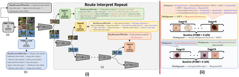
Figure 3: MoIE identifies diverse concepts for specific subsets of a class, unlike the generic ones by the baselines. (i) We construct the FOL explanations of the samples of, “Bay breasted warbler” in the CUB-200 dataset for VIT-based (a) CBM + E-LEN as an interpretable-by-design baseline, (b) PCBM + E-LEN as a posthoc baseline, (c) experts in MoIE at inference. We highlight the unique concepts for experts 1,2, and 3 in red, blue, and magenta, respectively. (ii) Comparison of FOL explanations by MoIE with the PCBM + E-LEN baselines for HAM10000 (top) and ISIC (down) to classify Malignant lesion. We highlight unique concepts for experts 3, 5, and 6 in red, blue, and violet, respectively. For brevity, we combine the local FOLs for each expert for the samples covered by them, shown in the figure.

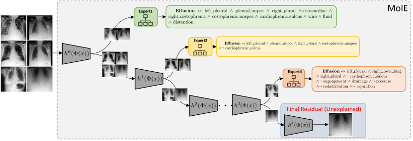
Figure 4: Construction logical explanations of the samples of “Effusion” in the MIMIC-CXR dataset for various experts in MoIE at inference. The final residual covers the unexplained sample, which is “harder” to explain (indicated in red).

Figure 5: Flexibility of FOL explanations by VIT-derived MoIE MoIE and the CBM + E-LEN and PCBM + E-LEN baselines for Awa2 dataset to classify “Otter” at inference. Both the baseline’s FOL constitutes identical concepts to distinguish all the samples. However, expert1 classifies “Otter” with hunter, group etc.as the identifying concept for the instances covered by it. Similarly expert5 classifies “Otter” using buckteeth, gray etc.. Note that, meat and gray are shared between the two experts. We highlight the shared concepts (artic) between the experts and the baselines as blue.

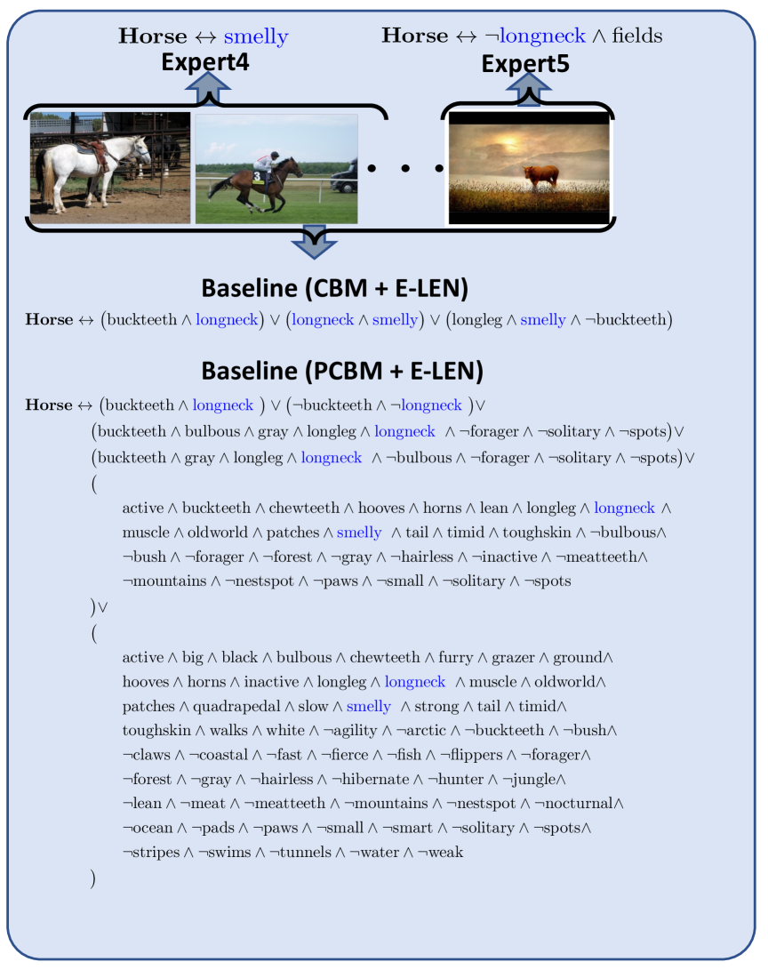
Figure 6: Flexibility of FOL explanations by VIT-derived MoIE MoIE and the CBM + E-LEN and PCBM + E-LEN baselines for Awa2 dataset to classify “Horse” at inference. Both the baseline’s FOL constitutes identical concepts to distinguish all the samples. However, expert4 classifies “Horse” with smelly as the identifying concept for the instances covered by it. Similarly, expert5 classifies the same “Horse” using longneck and fields. We highlight the shared concepts between the experts and the baselines as blue.

Heterogenity of Explanations: At each iteration of MoIE, the blackbox ($h^{k}(\Phi(.)$) splits into an interpretable expert ($g^{k}$) and a residual ($r^{k}$). Figure 3i shows this mechanism for VIT-based MoIE and compares the FOLs with CBM + E-LEN and PCBM + E-LEN baselines to classify “Bay Breasted Warbler” of CUB-200. The experts of different iterations specialize in specific instances of “Bay Breasted Warbler”. Thus, each expert’s FOL comprises its instance-specific concepts of the same class. For example, the concept, leg_color_grey is unique to expert4, but belly_pattern_solid and back_pattern_multicolored are unique to experts 1 and 2, respectively, to classify the instances of “Bay Breasted Warbler” in the  Figure 3(i)-c. Unlike MoIE, the baselines employ a single interpretable model $g$, resulting in a generic FOL with identical concepts for all the samples of “Bay Breasted Warbler” (Figure 3i(a-b)). Thus the baselines fail to capture the heterogeneity of explanations. Due to space constraints, we combine the local FOLs of different samples.

Figure 3ii shows such diverse local instance-specific explanations for HAM10000 (top) and ISIC (bottom). In Figure 3ii-(top), the baseline-FOL consists of concepts such as AtypicalPigmentNetwork and BlueWhitishVeil (BWV) to classify “Malignancy” for all the instances for HAM10000. However, expert 3 relies on RegressionStructures along with BWV to classify the same for the samples it covers. At the same time, expert 5 utilizes several other concepts e.g., IrregularStreaks, Irregular dots and globules (IrregularDG) etc. Due to space constraints, Figure 5 demonstrates similar results for the Awa2 dataset.

A.5 Identification of harder samples by successive residuals

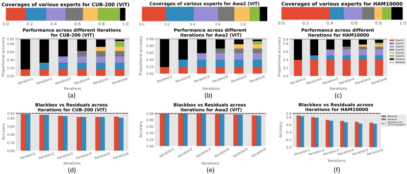
Figure 7: The performance of experts and residuals across iterations. (a-c) Coverage and proportional accuracy of the experts and residuals. (d-f) We route the samples covered by the residuals across iterations to the initial Blackbox $f^{0}$ and compare the accuracy of $f^{0}$ (red bar) with the residual (blue bar). Figures d-f show the progressive decline in performance of the residuals across iterations as they cover the samples in the increasing order of “hardness”. We observe the similar abysmal performance of the initial blackbox $f^{0}$ for these samples.

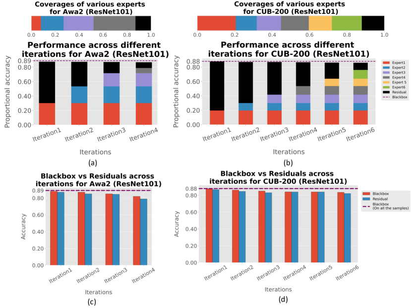
Figure 8: The performances of experts and residuals across iterations for ResNet derived MoIE for CUB-200 and Awa2. (a-b) Coverage and proportional accuracy of the experts and residuals. (c-d) We route the samples covered by the residuals across iterations to the initial Blackbox $f^{0}$ and compare the accuracy of $f^{0}$ (red bar) with the residual (blue bar).

Figure 7 (a-c) display the proportional accuracy of the experts and the residuals of our method per iteration. The proportional accuracy of each model (experts and/or residuals) is defined as the accuracy of that model times its coverage. Recall that the model’s coverage is the empirical mean of the samples selected by the selector. Figure 7a show that the experts and residual cumulatively achieve an accuracy $\sim$ 0.92 for the CUB-200 dataset in iteration 1, with more contribution from the residual (black bar) than the expert1 (blue bar). Later iterations cumulatively increase and worsen the performance of the experts and corresponding residuals, respectively. The final iteration carves out the entire interpretable portion from the Blackbox $f^{0}$ via all the experts, resulting in their more significant contribution to the cumulative performance. The residual of the last iteration covers the “hardest” samples, achieving low accuracy. Tracing these samples back to the original Blackbox $f^{0}$, it also classifies these samples poorly (Figure 7(d-f)). As shown in the coverage plot, this experiment reinforces Figure 1, where the flow through the experts gradually becomes thicker compared to the narrower flow of the residual with every iteration. Figure 8 shows the coverage (top row), performances (bottom row) of each expert and residual across iterations of - (a) ResNet101-derived Awa2 and (b) ResNet101-derived CUB-200 respectively.

References

- Ahuja et al. (2022) Ahuja, K., Caballero, E., Zhang, D., Gagnon-Audet, J.-C., Bengio, Y., Mitliagkas, I., and Rish, I. Invariance principle meets information bottleneck for out-of-distribution generalization, 2022.
- Arjovsky et al. (2020) Arjovsky, M., Bottou, L., Gulrajani, I., and Lopez-Paz, D. Invariant risk minimization, 2020.
- Barbiero et al. (2022) Barbiero, P., Ciravegna, G., Giannini, F., Lió, P., Gori, M., and Melacci, S. Entropy-based logic explanations of neural networks. In Proceedings of the AAAI Conference on Artificial Intelligence, volume 36, pp. 6046–6054, 2022.
- Belle (2020) Belle, V. Symbolic logic meets machine learning: A brief survey in infinite domains. In International Conference on Scalable Uncertainty Management, pp. 3–16. Springer, 2020.
- Besold et al. (2017) Besold, T. R., Garcez, A. d., Bader, S., Bowman, H., Domingos, P., Hitzler, P., Kühnberger, K.-U., Lamb, L. C., Lowd, D., Lima, P. M. V., et al. Neural-symbolic learning and reasoning: A survey and interpretation. arXiv preprint arXiv:1711.03902, 2017.
- Bissoto et al. (2020) Bissoto, A., Valle, E., and Avila, S. Debiasing skin lesion datasets and models? not so fast. In Proceedings of the IEEE/CVF Conference on Computer Vision and Pattern Recognition Workshops, pp. 740–741, 2020.
- Ciravegna et al. (2023) Ciravegna, G., Barbiero, P., Giannini, F., Gori, M., Lió, P., Maggini, M., and Melacci, S. Logic explained networks. Artificial Intelligence, 314:103822, 2023.
- Daneshjou et al. (2021) Daneshjou, R., Vodrahalli, K., Liang, W., Novoa, R. A., Jenkins, M., Rotemberg, V., Ko, J., Swetter, S. M., Bailey, E. E., Gevaert, O., et al. Disparities in dermatology ai: Assessments using diverse clinical images. arXiv preprint arXiv:2111.08006, 2021.
- Garcez et al. (2015) Garcez, A. d., Besold, T. R., De Raedt, L., Földiak, P., Hitzler, P., Icard, T., Kühnberger, K.-U., Lamb, L. C., Miikkulainen, R., and Silver, D. L. Neural-symbolic learning and reasoning: contributions and challenges. In 2015 AAAI Spring Symposium Series, 2015.
- Geifman & El-Yaniv (2019) Geifman, Y. and El-Yaniv, R. Selectivenet: A deep neural network with an integrated reject option. In International conference on machine learning, pp. 2151–2159. PMLR, 2019.
- Geirhos et al. (2020) Geirhos, R., Jacobsen, J.-H., Michaelis, C., Zemel, R., Brendel, W., Bethge, M., and Wichmann, F. A. Shortcut learning in deep neural networks. Nature Machine Intelligence, 2(11):665–673, 2020.
- Ghosh et al. (2023) Ghosh, S., Yu, K., Arabshahi, F., and Batmanghelich, K. Dividing and conquering a BlackBox to a mixture of interpretable models: Route, interpret, repeat. In Krause, A., Brunskill, E., Cho, K., Engelhardt, B., Sabato, S., and Scarlett, J. (eds.), Proceedings of the 40th International Conference on Machine Learning, volume 202 of Proceedings of Machine Learning Research, pp. 11360–11397. PMLR, 23–29 Jul 2023. URL https://proceedings.mlr.press/v202/ghosh23c.html.
- He et al. (2016) He, K., Zhang, X., Ren, S., and Sun, J. Deep residual learning for image recognition. In Proceedings of the IEEE conference on computer vision and pattern recognition, pp. 770–778, 2016.
- Huang et al. (2017) Huang, G., Liu, Z., Van Der Maaten, L., and Weinberger, K. Q. Densely connected convolutional networks. In Proceedings of the IEEE conference on computer vision and pattern recognition, pp. 4700–4708, 2017.
- Jain et al. (2021) Jain, S., Agrawal, A., Saporta, A., Truong, S. Q., Duong, D. N., Bui, T., Chambon, P., Zhang, Y., Lungren, M. P., Ng, A. Y., et al. Radgraph: Extracting clinical entities and relations from radiology reports. arXiv preprint arXiv:2106.14463, 2021.
- (16) Johnson, A., Lungren, M., Peng, Y., Lu, Z., Mark, R., Berkowitz, S., and Horng, S. Mimic-cxr-jpg-chest radiographs with structured labels.
- Kaushik et al. (2019) Kaushik, D., Hovy, E., and Lipton, Z. C. Learning the difference that makes a difference with counterfactually-augmented data. arXiv preprint arXiv:1909.12434, 2019.
- Kawahara et al. (2018) Kawahara, J., Daneshvar, S., Argenziano, G., and Hamarneh, G. Seven-point checklist and skin lesion classification using multitask multimodal neural nets. IEEE journal of biomedical and health informatics, 23(2):538–546, 2018.
- Kim et al. (2017) Kim, B., Wattenberg, M., Gilmer, J., Cai, C., Wexler, J., Viegas, F., and Sayres, R. Interpretability beyond feature attribution: Quantitative testing with concept activation vectors (tcav).(2017). arXiv preprint arXiv:1711.11279, 2017.
- Koh et al. (2020) Koh, P. W., Nguyen, T., Tang, Y. S., Mussmann, S., Pierson, E., Kim, B., and Liang, P. Concept bottleneck models. In International Conference on Machine Learning, pp. 5338–5348. PMLR, 2020.
- Krueger et al. (2021) Krueger, D., Caballero, E., Jacobsen, J.-H., Zhang, A., Binas, J., Zhang, D., Priol, R. L., and Courville, A. Out-of-distribution generalization via risk extrapolation (rex), 2021.
- Liu et al. (2021) Liu, E. Z., Haghgoo, B., Chen, A. S., Raghunathan, A., Koh, P. W., Sagawa, S., Liang, P., and Finn, C. Just train twice: Improving group robustness without training group information, 2021.
- Lu et al. (2021) Lu, M., Zhao, Q., Zhang, J., Pohl, K. M., Fei-Fei, L., Niebles, J. C., and Adeli, E. Metadata normalization. In Proceedings of the IEEE/CVF Conference on Computer Vision and Pattern Recognition, pp. 10917–10927, 2021.
- Lucieri et al. (2020) Lucieri, A., Bajwa, M. N., Braun, S. A., Malik, M. I., Dengel, A., and Ahmed, S. On interpretability of deep learning based skin lesion classifiers using concept activation vectors. In 2020 international joint conference on neural networks (IJCNN), pp. 1–10. IEEE, 2020.
- Rabanser et al. (2022) Rabanser, S., Thudi, A., Hamidieh, K., Dziedzic, A., and Papernot, N. Selective classification via neural network training dynamics. arXiv preprint arXiv:2205.13532, 2022.
- Ribeiro et al. (2016) Ribeiro, M. T., Singh, S., and Guestrin, C. ” why should i trust you?” explaining the predictions of any classifier. In Proceedings of the 22nd ACM SIGKDD international conference on knowledge discovery and data mining, pp. 1135–1144, 2016.
- Rosenzweig et al. (2021) Rosenzweig, J., Sicking, J., Houben, S., Mock, M., and Akila, M. Patch shortcuts: Interpretable proxy models efficiently find black-box vulnerabilities. In Proceedings of the IEEE/CVF Conference on Computer Vision and Pattern Recognition, pp. 56–65, 2021.
- Rotemberg et al. (2021) Rotemberg, V., Kurtansky, N., Betz-Stablein, B., Caffery, L., Chousakos, E., Codella, N., Combalia, M., Dusza, S., Guitera, P., Gutman, D., et al. A patient-centric dataset of images and metadata for identifying melanomas using clinical context. Scientific data, 8(1):1–8, 2021.
- Sagawa et al. (2019) Sagawa, S., Koh, P. W., Hashimoto, T. B., and Liang, P. Distributionally robust neural networks for group shifts: On the importance of regularization for worst-case generalization. arXiv preprint arXiv:1911.08731, 2019.
- Sagawa et al. (2020) Sagawa, S., Koh, P. W., Hashimoto, T. B., and Liang, P. Distributionally robust neural networks for group shifts: On the importance of regularization for worst-case generalization, 2020.
- Shi et al. (2021) Shi, Y., Seely, J., Torr, P. H. S., Siddharth, N., Hannun, A., Usunier, N., and Synnaeve, G. Gradient matching for domain generalization, 2021.
- Sun & Saenko (2016) Sun, B. and Saenko, K. Deep coral: Correlation alignment for deep domain adaptation, 2016.
- Szegedy et al. (2015) Szegedy, C., Liu, W., Jia, Y., Sermanet, P., Reed, S., Anguelov, D., Erhan, D., Vanhoucke, V., and Rabinovich, A. Going deeper with convolutions. In Proceedings of the IEEE conference on computer vision and pattern recognition, pp. 1–9, 2015.
- Tschandl et al. (2018) Tschandl, P., Rosendahl, C., and Kittler, H. The ham10000 dataset, a large collection of multi-source dermatoscopic images of common pigmented skin lesions. Scientific data, 5(1):1–9, 2018.
- Wadden et al. (2019) Wadden, D., Wennberg, U., Luan, Y., and Hajishirzi, H. Entity, relation, and event extraction with contextualized span representations. In Proceedings of the 2019 Conference on Empirical Methods in Natural Language Processing and the 9th International Joint Conference on Natural Language Processing (EMNLP-IJCNLP), pp. 5784–5789, Hong Kong, China, November 2019. Association for Computational Linguistics. doi: 10.18653/v1/D19-1585. URL https://aclanthology.org/D19-1585.
- Wah et al. (2011) Wah, C., Branson, S., Welinder, P., Perona, P., and Belongie, S. The caltech-ucsd birds-200-2011 dataset. 2011.
- Wang et al. (2021) Wang, J., Yu, X., and Gao, Y. Feature fusion vision transformer for fine-grained visual categorization. arXiv preprint arXiv:2107.02341, 2021.
- Xian et al. (2018) Xian, Y., Lampert, C. H., Schiele, B., and Akata, Z. Zero-shot learning—a comprehensive evaluation of the good, the bad and the ugly. IEEE transactions on pattern analysis and machine intelligence, 41(9):2251–2265, 2018.
- Xu et al. (2020) Xu, M., Zhang, J., Ni, B., Li, T., Wang, C., Tian, Q., and Zhang, W. Adversarial domain adaptation with domain mixup. Proceedings of the AAAI Conference on Artificial Intelligence, 34(04):6502–6509, Apr. 2020. doi: 10.1609/aaai.v34i04.6123. URL https://ojs.aaai.org/index.php/AAAI/article/view/6123.
- Yao et al. (2022) Yao, H., Wang, Y., Li, S., Zhang, L., Liang, W., Zou, J., and Finn, C. Improving out-of-distribution robustness via selective augmentation. In Chaudhuri, K., Jegelka, S., Song, L., Szepesvari, C., Niu, G., and Sabato, S. (eds.), Proceedings of the 39th International Conference on Machine Learning, volume 162 of Proceedings of Machine Learning Research, pp. 25407–25437. PMLR, 17–23 Jul 2022. URL https://proceedings.mlr.press/v162/yao22b.html.
- Yu et al. (2022) Yu, K., Ghosh, S., Liu, Z., Deible, C., and Batmanghelich, K. Anatomy-guided weakly-supervised abnormality localization in chest x-rays. arXiv preprint arXiv:2206.12704, 2022.
- Yuksekgonul et al. (2022) Yuksekgonul, M., Wang, M., and Zou, J. Post-hoc concept bottleneck models. arXiv preprint arXiv:2205.15480, 2022.
- Zarlenga et al. (2022) Zarlenga, M. E., Barbiero, P., Ciravegna, G., Marra, G., Giannini, F., Diligenti, M., Shams, Z., Precioso, F., Melacci, S., Weller, A., et al. Concept embedding models. arXiv preprint arXiv:2209.09056, 2022.