Thermal Analysis of Malignant Brain Tumors by Employing a Morphological Differentiation-Based Method in Conjunction with Artificial Neural Network

Abstract

In this study, a morphological differentiation-based method has been introduced which employs temperature distribution on the tissue surface to detect brain tumor’s malignancy. According to the common tumor CT scans, two different scenarios have been implemented to describe irregular shape of the malignant tumor. In the first scenario, tumor has been considered as a polygon base prism and in the second one, it has been considered as a star-shaped base prism. By increasing the number of sides of the polygon or wings of the star, degree of the malignancy has been increased. Constant heat generation has been considered for the tumor and finite element analysis has been conducted by the ABAQUS software linked with a PYTHON script on both tumor models to study temperature variations on the top tissue surface. This temperature distribution has been characterized by 10 parameters. In each scenario, 98 sets of these parameters has been used as inputs of a radial basis function neural network (RBFNN) and number of sides or wings has been selected to be the output. The RBFNN has been trained to identify malignancy of tumor based on its morphology. According to the RBFNN results, the proposed method has been capable of differentiating between benign and malignant tumors and estimating the degree of malignancy with high accuracy.

Keywords Brain tumor $\cdot$ Tumor differentiation $\cdot$ Morphological analysis $\cdot$ Artificial neural network $\cdot$ Finite element method

1 Introduction

Brain tumors are categorized into benign and malignant. Despite considerable advances in the diagnosis and the treatment of the brain tumors, the mortality from malignant brain tumors is still high Kateb et al. (2009). Malignant tumors are cancerous and are made up of cells that grow out of control Baish and Jain (2000). It has been found that cells in the peripheral areas of the malignant tumor have a high invasive rhythm to the surrounding tissue Guarino et al. (2007). Therefore, border of a malignant tumor has sharp edges that result in a polygonal shape or star-shaped morphology of the tumor Golston et al. (1992). Malignant tumors are deeply fixed in the surrounding tissue by the sharp edges. The sharpness increases rapidly since the tumor needs more invasions to the nearby tissue for the growth Condeelis and Pollard (2006). On the contrary, benign tumors are often smooth and round and easy to remove since they are not attached to the surrounding tissue Shah et al. (1995).
Surgery is usually the first step in the treatment of the brain tumors. The goal is to remove as much of the tumor as possible while maintaining neurological function. Surgical treatments for malignant brain tumors are not easy to handle because they do not have clear borders Argani et al. (2001). In order to improve the surgeon’s ability in defining the tumor’s border and avoid injury to vital brain areas in the operating room, image-guided surgery is performed. Intraoperative imaging is a revolutionary tool in the modern neurosurgery Illingworth (1995). Intraoperative imaging techniques especially intraoperative MRI (iMRI), help neurosurgeons achieve the goal of maximum tumor resection with least morbidity Schulder and Carmel (2003). The main drawbacks of using iMRI is the patient positioning during the surgery for a proper imaging and also limitation of using the surgical instruments because of the presence of a strong magnetic field.
In order to avoid limitations and high expenses of intraoperative imaging, many researches have focused on improving the performance of the preoperative tumor imaging techniques. These techniques mainly include magnetic resonance imaging (MRI) and computed tomography scan (CT scan). In the MRI, an injected contrast agent is used which makes the cancerous tumor brighter than the surrounding normal tissue. During the scan, there is a rapid increase in the signal intensity of a malignant tumor immediately 1 to 2 minutes after the injection. The intensity decreases in the following minutesKobayashi and Brechbiel (2005). For a benign mass, the rise in the intensity is much slower. Inaccuracy in the time and the intensity measurements results in a probability that benign and malignant tumors have overlap in their morphological appearance Barentsz et al. (1996). It was proved that the specificity of MRI to correctly predict a benign tumor is limited. Moreover, Specificity of MRI would be decreased by reducing the tumor size. Therefore, MRI is usually recommended after a malignancy is detected by other methods in order to have more information about the extent of the cancer.
CAT or CT scanning is an accurate medical test that combines x-ray with computerized technology to detect malignancy. The main drawback of this method is using high doses of radiation, leading to the possibility of lung cancer or breast cancer as a consequence Lee et al. (2004). X-rays also damage DNA itself Spotheim-Maurizot and Davidkova (2011). CT scanning provides images in shades of grey; occasionally the shades are similar, making it difficult to distinguish between the normal and abnormal tissues. To overcome such deficiency a contrast agent may be injected into the bloodstream. Main problems of the injection include pathological side-effects such as nausea and vomiting, hypotension and extravasation of the contrast which can be severe enough to require skin grafting Rull and Tidy (2015).
During recent years, many researches have focused on improving the procedure of defining tumor morphology in the preoperative imaging techniques. Wu et al. (2012) used the level set method to segment ultrasound breast tumors automatically and used a genetic algorithm to detect indicative features for the support vector machine (SVM) to detect tumor malignancy. The proposed system could discriminate benign from malignant breast tumors with high accuracy and short feature extraction time. Huang et al. (2013) evaluated the value of using 3D breast MRI morphological features to differentiate malignant and benign breast tumor. Malignancy of a tumor was investigated by using a number of extracted morphological features in the breast MRI. Jen and Yu (2015) introduced a method for abnormality detection in the mammograms based on an abnormality detection classifier (ADC) which extracts a couple of distinctive features including first-order statistical intensities and gradients. In this method, image preprocessing techniques were used to obtain more accurate breast tissue segmentation. Han et al. (2015) provided an improved segmentation algorithm which is a combination of the fuzzy clustering segmentation and the fuzzy edge enhancement. Results showed that the fuzzy clustering segmentation is highly efficient for complex brain tissues, and the images after the fuzzy clustering segmentation provide a solid foundation for 3D processing and help to acquire better 3D visualization of the brain tumors. Ramya and Sasirekha (2015) developed a robust segmentation algorithm in order to diagnose tumors in the MR images. In this method, a 4th-order partial differential equation was employed to denoise images to improve segmentation accuracy. Zhang et al. (2016) proposed a wavelet energy-based method to classify the MR images. This approach had a three-stage system which detects characteristics indicative of the abnormal brain tissues. Shirazi and Rashedi (2016) used a combination of support vector machine (SVM) and mixed gravitational search algorithm (MGSA) to improve the classification accuracy in the mammography images. Xia et al. (2016) proposed a novel voting ranking random forests (VRRF) method for the image classification and developed a center-proliferation segmentation (CPS) method. This method showed good performance in the image classification with strong robustness.
In the present study, a palpation-based method was used for scanning of the brain tissue in order to detect and follow the malignancies. The method avoids the main aforementioned drawbacks of the imaging techniques since it is only based on the tissue palpation. It is called “tactile thermography” and maps the thermal parameters of the tissue mainly the temperature and the heat flux on the tissue surface. Sadeghi-Goughari and Mojra (2015) estimated thermal parameters of the brain tumors by introducing the tactile thermography method as a new noninvasive thermal imaging method. In this method, the brain tissue was mechanically and thermally loaded and the temperature and the heat flux variations on the tissue surfaces were recorded. A number of thermal parameters were extracted and optimized by an artificial neural network to verify tumor existence and its depth. The main objective of this study is to evaluate the capability of the proposed method in detecting sharp morphology of the tumor indicative of the tumor malignancy and also to verify its sensitivity to the sharpness increase that can be used in the follow-up procedure for evaluating the tumor growth.
To this end, a malignant tumor is simulated in the brain tissue by two scenarios that represent the invading sharp edges of the tumor. Moreover, the tumor is considered as a heat source in the thermal analysis since the cell number and the overall cell metabolism are considerably increased in the tumor relative to the normal tissue. By conducting a thermal analysis, the temperature distribution on the tissue surface is obtained for tumors with varying penetration into the surrounding tissue. By the use of the artificial neural network, a number of variables are extracted from the temperature map and will be used as the malignancy indicative features.

2 Materials and Methods

Figure 1 and Figure 2 are CT scan images of two malignant brain tumors. It can be inferred that while a benign tumor has an almost smooth round shape, malignancy can be identified by the existence of invading edges. Two major morphologies of the malignant brain tumors are identified by solid lines in Figure 1 and Figure 2. The first morphology resembles a polygonal shape while the second one resembles a star. In the present numerical analysis, the tumor malignancy was simulated in two different scenarios:

1. Tumor was considered as an n-sided polygonal based prism. Area of the polygonal base and consequently the volume of the tumor and the distance of uppermost vertex (D) were kept unchanged for all number of sides (n) (Figure 3).

2. Tumor was considered as a star polygonal based prism. This star was formed by an inscribed circle with constant radius of R=10mm and different corner vertices. Tumor penetration inside the nearby tissue was increased by increasing the number of corner vertices. Each group of two intersecting edges was called a wing. The number of wings was increased by keeping the star polygonal base area constant (and the tumor volume) (Figure 4).

Table 1: Dimensions of simulated tissue containing a malignant tumor, all dimensions are in millimeters.

X	Y	Z	D	R
120	60	25	12	10

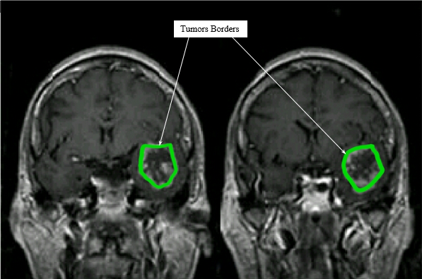
Figure 1: CT scan image of a malignant tumor resembles a polygon presented as scenario 1.

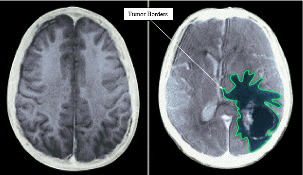
Figure 2: CT scan image of a malignant tumor resembles a star presented as scenario 2.

(a)

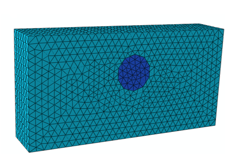
(b)

Figure 3: Mid cross section of the brain tissue model (rectangular cuboid) in the ABAQUS environment including (a) a pentagonal based prismatic tumor; (b) a decagonal based prismatic tumor.

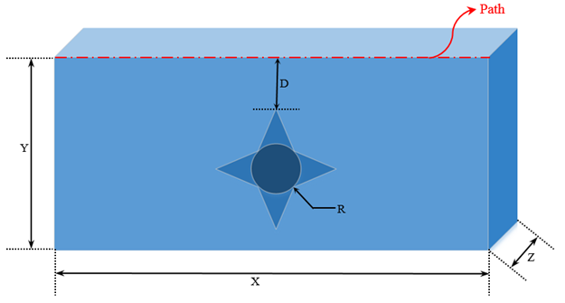
(a)

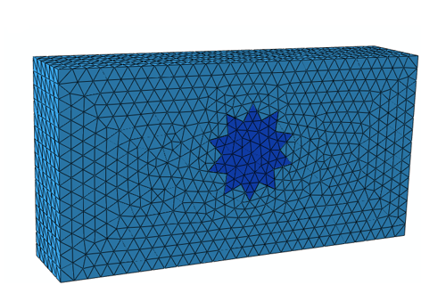
(b)

Figure 4: Mid cross section of the brain tissue model (rectangular cuboid) in the ABAQUS environment including (a) a 4 wing star polygonal based prismatic tumor; (b) a 10 wing star polygonal based prismatic tumor.

Geometrical dimensions of the sample brain tissue containing a malignant tumor is presented in Table 1. In order to describe mechanical behavior of the brain tissue, the elasticity parameters of the brain tissue obtained by Soza et al. (2005)) were used(Table 2). The Young’s modulus of tumor was considered to be 10 times of the brain tissue while the Poisson’s ratio was the same Shiddiqi et al. (2010).

Table 2: Elastic properties of the brain tissue.

Young’s modulus (Pa)	Poisson’s ratio
9210.87	0.458344

Study of energy transport in the biological systems involves various mechanisms including conduction, advection and metabolism Gore and Surawicz (2003). In this study these phenomena were considered in a steady-state thermal analysis; a constant thermal conductivity equal to 0.6 W/m2K was considered for the brain tissue Elwassif et al. (2006), blood perfusion and metabolic activities were considered by assuming a constant heat generation equal to 100000 W/m3 for the tumor. A convective heat transfer between the top tissue surface and the surrounding environment was considered with a convective heat transfer coefficient equals 20 W/m2K. The bottom surface of the brain tissue sample was assumed to have a constant temperature of 33.1°C equal to the temperature of the blood vessel which was assumed to be in contact with the tissue. Side surfaces were insulated.
ABAQUS software (version 6.14) was employed to perform finite element analysis (FEA) under 3D axisymmetric conditions. A compressive strain was applied to the top surface of the tissue and the temperature variation was recorded on it. In order to measure temperature variations while the tissue was loaded mechanically, the step named “COUPLED TEMP-DISPLACEMENT” was selected. A “time increment” and a “time period” should be assigned to the step for that the default values were assumed. For both rectangular cube and prism, a 4-noded tetrahedral with thermal coupling (C3D4T) element type was used.
Rather than thermal boundary conditions, mechanical boundary conditions were also defined. The bottom surface of the tissue was totally fixed while the top surface was loaded by a compressive strain equals to 6% which corresponds to a 4 mm compression. Adhesion of the malignant tumor to its surrounding tissue was satisfied by applying ‘TIE’ constraint between the brain tissue and the tumor.
Mesh independency was examined for the tissue sample including a decagonal based prismatic tumor. Three stages of mesh refinement were performed and temperature values were measured. For three models with 21796, 29725 and 44029 elements, the computational time was 19.27, 23.44 and 29.82 seconds, respectively. The maximum relative difference between the temperature values in the models with 21796 elements and 29725 elements was less than 1%, so the computational grid with 21796 elements was selected (Table 3).

Table 3: Mesh independency evaluation for the sample brain tissue including a malignant tumor.

decagonal based prismatic tumor				10 wing star polygonal based prismatic tumor
Number of elements	Element type	Maximum error relative to selected model (%)	Computational time (sec)	Number of elements	Element type	Maximum error relative to selected model (%)	Computational time (sec)
21796	C3D4T	0	19.27	22362	C3D4T	0	21.49
29725	C3D4T	0.0751	23.44	29869	C3D4T	0.0665	23.56
44029	C3D4T	0.0382	29.82	43366	C3D4T	0.0269	30.81

Similarly, mesh independency was examined for the tissue sample including the star polygonal based prismatic tumor with 10 wings. For three models with 22362, 29869 and 43366 elements, the computational time was 21.49, 23.56 and 30.81 seconds, respectively. The maximum relative error between the temperature values in the models with 22362 elements and 29869 elements was less than 1%, so the computational mesh with 22362 elements was selected (Table 3).
The sample model of the brain tissue was numerically analyzed while a tumor with irregular borders was included as a prism with a polygonal base or a star polygonal base. The number of sides of the polygon and wings of the star were changed to the study the effects of the irregularity increase on the thermal parameters. Table 4 lists the number of sides and wings of the tumor model. A total number of 98 polygonal based prisms and 98 star polygonal based prisms were modeled and analyzed by the ABAQUS software linked with a PYTHON script to automatically change the number of sides and wings. MATLAB software (version 8.6) was used to plot the thermal outputs and extract thermal variables that would be employed as the inputs of an artificial neural network.

Table 4: Number of sides and wings of both tumor models.

Initial value	Increment	Final value
3	1	100

2.1 Artificial neural network

Artificial neural networks (ANNS) try to model the processing capabilities of actual human nervous systems. They are consist of numerous simple computing components, called neurons that generates an input layer, one or more hidden layers and an output layer Steuber and Jaeger (2013). ANNs are mostly used for functions approximation which may be single variable or multivariable. In order to recognize inputs patterns, suitable weights for the connections must be derived. Therefore, the network should be trained to obtain proper desired results.
In this study, radial base function neural network (RBF) was used that employs the radial basis functions as the activation functions Park and Sandberg (1991). The output of this network is a linear combination of neuron parameters and radial basis function of the inputs. Properties of the employed network are listed in Table 5.

Table 5: Neural network’s properties

Performance function	Network initialization function	Network derivative function	Number of inputs	Number of outputs	Transfer function	Type of neurons in 1st layer	Type of neurons in 2nd layer	Number of epochs
MSE	initlay	defaultderiv	10	1	Tansig	Radbas	Purelin	100

Performance of this network was evaluated by mean squared error (MSE) that is the average of the squares of the errors and error is the difference between the desired value of a variable and the estimated value by the network (equation 3). The ideal performance of a neural network occurs when values of the MSE are zero. The error is defined as equation 1:

$$e_{i}=\hat{x}_{i}-x_{i}$$ (1)

Where $\hat{x}_{i}$ is the estimated value and $x_{i}$ is the desired value that is obtained from the ABAQUS runs in this study. Mean of the errors for all data (98 data for each tumor model) is then calculated by equation 2:

$$\mu=\frac{1}{n}\sum_{i=1}^{n}e_{i}$$ (2)

$$MSE=\frac{1}{n}\sum_{i=1}^{n}e_{i}^{2}$$ (3)

Where $n$ is the number of the network inputs. The variance is the average of the squared differences from the mean (equation 4):

$$\sigma^{2}=\frac{1}{n}\sum_{i=1}^{n}(e_{i}-\mu)^{2}$$ (4)

In order to have a better criterion for evaluating the network performance, it’s better to use the root mean square error (RMSE) which has the same unit as the variable being estimated (equation 5). The square root of the variance is known as the standard deviation (equation 6).

$$RMSE=\sqrt{\frac{1}{n}\sum_{i=1}^{n}e_{i}^{2}}$$ (5)

$$\sigma=\sqrt{\frac{1}{n}\sum_{i=1}^{n}(e_{i}-\mu)^{2}}$$ (6)

3 Results and Discussion

Figure 5 is a display of the temperature contours in the mid cross section of the model obtained from the ABAQUS runs. Tumor existence in the tissue increases the temperature in the vicinity of the tumor. At further distance from the tumor margin, the temperature reduces and the rate of reduction is not proportional to the distance from the tumor center. Temperature gradients are considerable in the tumor vicinity. It can be also inferred from Figure 7 that the area of the tumor-affected region depends on the tumor shape to a great extent. While the tumor effect spreads smoothly over the whole tissue area for a polygonal based prismatic tumor, it has a localized distribution for a star polygon. Consequently, temperature distribution pattern can be correlated with the shape of the malignant tumor.

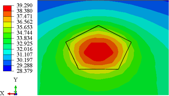
(a)

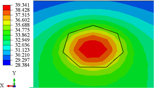
(b)

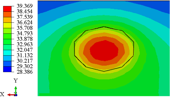
(c)

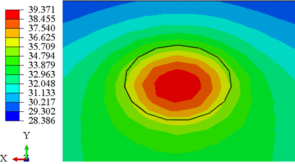
(d)

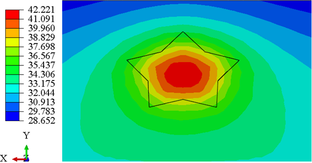
(e)

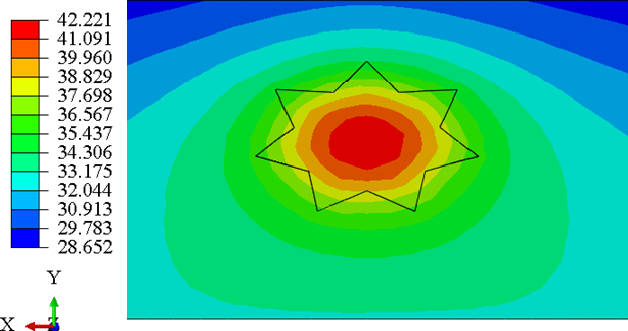
(f)

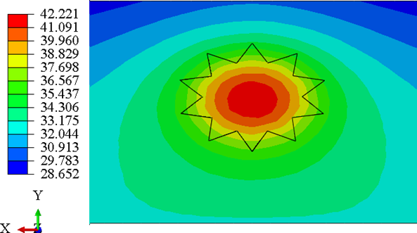
(g)

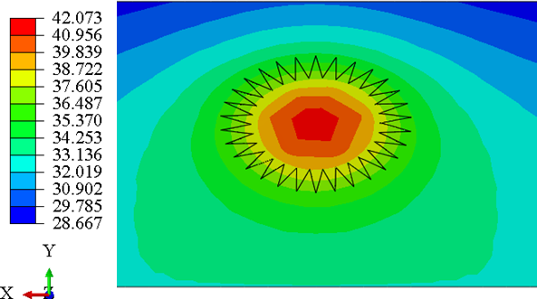
(h)

Figure 5: Temperature contours in the mid cross section of the brain tissue model including: a pentagonal, heptagonal, decagonal and 15 sided polygonal based prismatic tumor (top from left to right) and a 5 wing, 7 wing, 10 wing, and 30 wing star polygonal based prismatic tumor (bottom from left to right).

Temperature variation was studied on the paths defined in Figure 3(a) and Figure 4a. and by varying the number of sides and wings of the tumor (Figure 4(a). The diagrams show that the location of the maximum temperature on the tissue surface corresponds to the location of the tumor center inside the tissue where the tumor distance is the minimum relative to the tissue surface. Moreover, while the tumor volume was kept unchanged, increasing the number of sides and wings results in the elevation of the maximum surface temperature. These achievements offer two opportunities:

1. The temperature variation is indicative of the tumor existence. Therefore, temperature map can be used for the tumor detection task.

2. For a specific malignant tumor, the temperature map can be recorded in the successive examinations. Comparison between the maps can be indicative of the malignancy progression in a period of time.

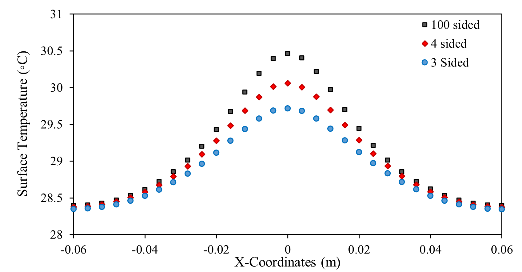
(a)

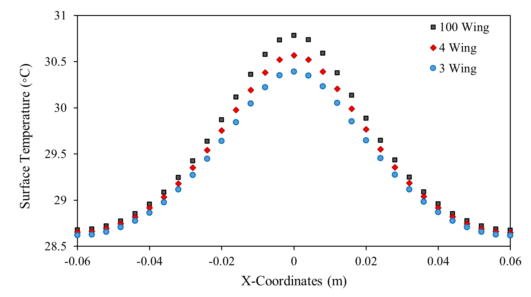
(b)

Figure 6: Temperature distribution on a path which passes from the center of the top tissue surface for brain tissue sample including a) polygonal based prismatic tumors; b) star polygonal based prismatic tumors.

In Figure 7 variation of the maximum temperature on the tissue surface is investigated by increasing the number of sides and wings. For the polygonal based tumor model, increase of the number of sides from 3 to 100 results in the elevation of the maximum surface temperature from 29.7°C to 30.5°C. For the star polygonal based tumor, by increasing the number of the wings from 3 to 100, maximum surface temperature increases from 30.3°C to 30.8°C. However, maximum temperature variations are less than 0.02°C and 0.01°C by increasing the number of sides and wings more than 20, respectively. Therefore, sensitivity of the surface temperature to the variation of the sides and wings of the tumor reduces when the sharpness of the tumor morphology increases.

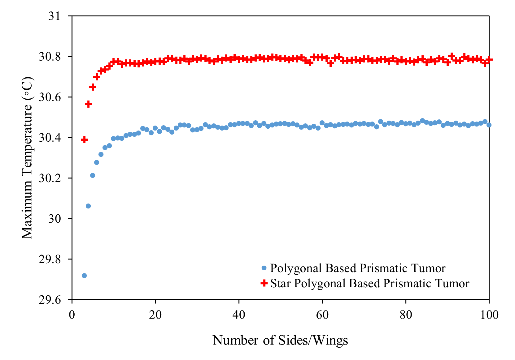
Figure 7: Correlation between the maximum surface temperature and number of sides of the polygonal based prismatic tumor and number of wings of the star polygonal based prismatic tumor.

In order to find a quantitative criterion for the tumor detection and the malignancy progression, the temperature curve on the tissue surface was interpolated by a 4th-order Fourier series (equation 7). Fitting error was less than 1% for all tumor models. By fitting this curve to each set of data achieved from the ABAQUS runs, 10 coefficients were extracted for each tumor which are $a_{i}^{\prime}$ s,$b_{i}^{\prime}$ s and w in equation 7.

$$T(x)=a_{0}+\sum_{i=1}^{4}(a_{i}coswx+b_{i}sinwx)$$ (7)

These coefficients were used as the inputs of a radial basis function (RBF) artificial neural network (ANN). This network (RBFNN) provided the link between the inputs that were the surface temperature interpolating function’s coefficients and outputs that were the corresponding number of sides or wings of the malignant tumor.

3.1 Polygonal based prismatic tumor

The RBFNN was trained to estimate number of sides by using 98 samples of the brain tissue including a polygonal based prismatic tumor with different number of sides of the polygonal base. 68 samples from the whole datasets were used randomly for training the network and 30 remaining samples were used for the testing procedure.

For a better comprehension of the extent and the distribution of the coefficients of equation 7, the mean $\bar{x}$ the minimum $x_{min}$, and maximum $x_{max}$ of these coefficients for the polygonal base tumor model are listed in Table 6. The employed neural network transfer function was "Tansig"that takes values only between $-1$ and $1$. Therefore, the coefficients were normalized in the range of $[-11]$. Normalization of the dataset would prevent misinterpretation in defining the contribution of each input in the neural network.

Table 6: Variation of the Fourier series coefficients for the polygonal based prismatic tumor.

Coefficient	$x_{min}$	$\bar{x}$	$x_{max}$
$a_{0}$	28.8860	29.1522	29.1666
$a_{1}$	0.6511	0.9437	0.9583
$a_{2}$	0.1349	0.2394	0.2462
$a_{3}$	0.0326	0.0701	0.0737
$a_{4}$	0.0101	0.0203	0.0223
$b_{1}$	0.0017	0.0042	0.0062
$b_{2}$	0.000983	0.0034	0.0059
$b_{3}$	-0.000574	0.0018	0.0043
$b_{4}$	-0.000914	0.0010	0.0031
$w$	51.7375	52.6726	53.0506

The box plot of the normalized coefficients is plotted in Figure 8 that is a standardized way of displaying the distribution of data based on five characteristics: minimum, maximum, median, first quartile, and third quartile. In a box plot, the rectangle expands from the first quartile to the third quartile and the inner line represents the median. A segment inside the rectangle shows the median and whiskers above and below the box show the minimum and the maximum of the data. It can be inferred from Figure10 that $a_{0}$,$a_{1}$,$a_{2}$ and $a_{3}$ have the most compact distributions which means that these coefficients are not too sensitive to the variation of the number of sides and consequently do not have major contribution in the proposed network training. Contribution of these coefficients in the network is providing a general similarity between the patterns of temperature variations. On the contrary, $b_{1}$,$b_{3}$ and $b_{4}$ have the widest distributions. Moreover, based on the position of the median, a coefficient may have normal or abnormal distribution. According to the box plot, $a_{2}$,$a_{4}$, $b_{3}$, and $b_{4}$ have the most normal distributions that mean that by varying the number of sides, distribution of these coefficients is not concentrated below or above the medians. Normal distribution facilitates the network training and reduces the normal deviations. Distribution of $a_{0}$, $a_{1}$ and $a_{3}$ are far from being normal.

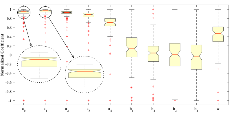
Figure 8: Box plot of the normalized coefficients for the polygon base prismatic tumor.

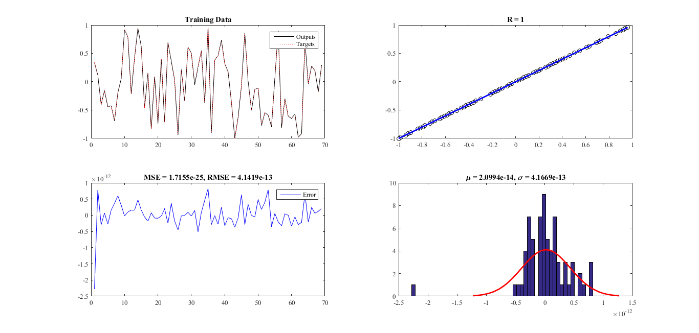
Figure 9: Performance plots of data training by the proposed RBFNN for the polygonal based prismatic tumor.

Performance of the proposed RBFNN in data training was evaluated by four different plots in Figure9. The top left figure is a plot of the network output that has overlap with the corresponding real values. The top right figure is a plot the linear regression of the real or desired values versus the network outputs. Slope of the fitted line by the RBFNN was close to 1 that means that the estimated values are very close to the real values. RMSE was equal to $4.142×10^{-13}$. Table 7 provides the value of the evaluating parameters for both training and testing datasets.

Table 7: Evaluating parameters of the proposed RBFNN for the polygonal based prismatic tumor.

Training dataset			Testing dataset
RMSE	$\mu$	$\sigma$	RMSE	$\mu$	$\sigma$
$4.142×10^{-13}$	$2.099×10^{-14}$	$4.167×10^{-13}$	$3.310×10^{-12}$	$-1.937×10^{-12}$	$2.727×10^{-12}$

3.2 Star polygonal based prismatic tumor

For the second tumor model, the RBFNN was trained to estimate the number of tumor wings by using 98 samples of the tissue including star polygonal based prismatic tumors. Number of the training and testing datasets were 68 and 30, respectively. Mean $\bar{x}$ , minimum $x_{mean}$ , and maximum $x_{max}$ of the extracted coefficients are listed in Table 8.

Table 8: Variation of the Fourier series coefficients for the star polygonal based prismatic tumor.

Coefficient	$x_{min}$	$\bar{x}$	$x_{max}$
$a_{1}$	0.8480	1.0025	1.0119
$a_{2}$	0.1652	0.2044	0.2118
$a_{3}$	0.0370	0.0441	0.0470
$a_{4}$	0.0087	0.0124	0.0155
$b_{1}$	0.0015	0.0039	0.0060
$b_{2}$	0.00019	0.0030	0.0055
$b_{3}$	-0.0015	0.0012	0.0043
$b_{4}$	-0.0019	0.0007	0.0044
$w$	51.2349	51.6295	52.1607

The box plot of the normalized coefficients is plotted in Figure 10. Similar to the polygonal based prismatic tumor, the box plot shows that $a_{0}$,$a_{1}$,and $a_{2}$ have the most compact distributions and $a_{4}$, $b_{1}$ and $b_{2}$ have the most normal distributions.

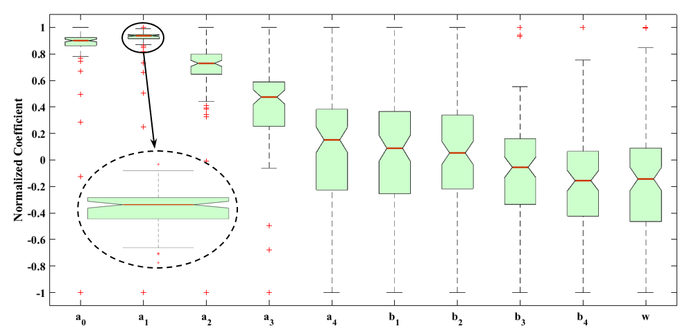
Figure 10: Box plot of the normalized coefficients for the star-shaped base prismatic tumor.

Performance of the RBFNN was evaluated by the prescribed parameters for both training and testing datasets (Table9). For both malignant tumor models, R-value was close to 1 and insignificant values of RMSE are indicative of perfect fit of the designed network to the numerical data. RMSE, errors mean ($\mu$) and standard deviation ($\sigma$) are almost zero.

Table 9: Evaluating parameters of the proposed RBFNN for the star polygonal based prismatic tumor.

Training dataset			Testing dataset
RMSE	$\mu$	$\sigma$	RMSE	$\mu$	$\sigma$
$7.028×10^{-13}$	$-2.099×10^{-13}$	$6.742×10^{-13}$	$2.846×10^{-12}$	$1.987×10^{-12}$	$2.072×10^{-12}$

4 Conclusion

In the present study, a morphologically malignant tumor was simulated in a cuboid sample of the brain tissue and thermal effect of the tumor on the surrounding tissue was investigated. Considering CT-scan images, morphology of the malignant tumor was defined by two major scenarios; polygonal based prismatic tumor and star polygonal based prismatic tumor. Main characteristic of both morphologies is having corner vertices and multiple edges. The tumor was considered as a biological heat source in the tissue and the temperature map on the tissue surface was obtained. An interpolating function was fitted to the temperature map and ten distinct variables were extracted. The tumor growth and malignancy progression was linked to the increase of the corner vertices of the tumor. Subsequently, 98 polygonal based prismatic tumors with different number of sides and 98 star polygonal based prismatic tumors with different number of wings were modeled and thermally analyzed. The aforementioned variables were extracted for all tumor models. Numerical results showed that the temperature of the normal tissue is affected by the tumor existence and the pattern of temperature variation has agreement with the tumor morphology. Moreover, the extracted thermal variables for all tumor models were used as the inputs of a radial base function neural network (RBFNN) and the number of sides and wings were estimated. The RBFNN analysis offered that the proposed method has the potential to be employed as a quantitative tool for measuring the malignancy progression over time.

References

- Kateb et al. [2009] Babak Kateb, Vicky Yamamoto, Cheng Yu, Warren Grundfest, and John Peter Gruen. Infrared thermal imaging: A review of the literature and case report. NeuroImage, 47:T154—-T162, 2009. ISSN 10538119. doi:10.1016/j.neuroimage.2009.03.043. URL http://dx.doi.org/10.1016/j.neuroimage.2009.03.043.
- Baish and Jain [2000] J W Baish and R K Jain. Fractals and cancer. Cancer Research, 60:3683–3688, 2000. ISSN 00085472. doi:10.1016/0306-9877(94)90163-5.
- Guarino et al. [2007] Marcello Guarino, Barbara Rubino, and Gianmario Ballabio. The role of epithelial-mesenchymal transition in cancer pathology. Pathology, 39:305–318, 2007. ISSN 1465-3931. doi:10.1080/00313020701329914. URL http://dx.doi.org/10.1080/00313020701329914.
- Golston et al. [1992] Jeremiah E Golston, William V Stoecker, Randy H Moss, and Inder P S Dhillon. Automatic detection of irregular borders in melanoma and other skin tumors. Computerized Medical Imaging and Graphics, 16:199–203, 1992. ISSN 08956111. doi:10.1016/0895-6111(92)90074-J. URL http://dx.doi.org/10.1016/0895-6111(92)90074-j.
- Condeelis and Pollard [2006] John Condeelis and Jeffrey W Pollard. Macrophages: Obligate partners for tumor cell migration, invasion, and metastasis. Cell, 124:263–266, 2006. ISSN 00928674. doi:10.1016/j.cell.2006.01.007. URL http://dx.doi.org/10.1016/j.cell.2006.01.007.
- Shah et al. [1995] H Shah, L Garbe, E Nussbaum, J F Dumon, P L Chiodera, and S Cavaliere. Benign tumors of the tracheobronchial tree: Endoscopic characteristics and role of laser resection. Chest, 107:1744–1751, 1995. ISSN 00123692. doi:10.1378/chest.107.6.1744. URL http://dx.doi.org/10.1378/chest.107.6.1744.
- Argani et al. [2001] Pedram Argani, Cristina R Antonescu, Peter B Illei, Man Yee Lui, Charles F Timmons, Robert Newbury, Victor E Reuter, A Julian Garvin, Antonio R Perez-atayde, Jonathan A Fletcher, J Bruce Beckwith, Julia A Bridge, and Marc Ladanyi. Primary renal neoplasms with the. The American Journal of Pathology, 159:179–192, 2001. ISSN 00029440. doi:10.1016/S0002-9440(10)61684-7. URL http://dx.doi.org/10.1016/S0002-9440(10)61684-7.
- Illingworth [1995] Rd Illingworth. Minimally Invasive Neurosurgery II, volume 59. Springer, 1995. ISBN 978-1-58829-147-9. doi:10.1136/jnnp.59.2.220-b. URL http://dx.doi.org/10.1385/1592598994.
- Schulder and Carmel [2003] Michael Schulder and Peter W Carmel. Intraoperative magnetic resonance imaging: impact on brain tumor surgery. Cancer control : journal of the Moffitt Cancer Center, 10:115–124, 2003. ISSN 1073-2748. URL http://www.ncbi.nlm.nih.gov/pubmed/12712006.
- Kobayashi and Brechbiel [2005] Hisataka Kobayashi and Martin W Brechbiel. Nano-sized mri contrast agents with dendrimer cores. Advanced Drug Delivery Reviews, 57:2271–2286, 2005. ISSN 0169409X. doi:10.1016/j.addr.2005.09.016. URL http://dx.doi.org/10.1016/j.addr.2005.09.016.
- Barentsz et al. [1996] J O Barentsz, G J Jager, J A Witjes, J H J Ruijs, and J A Witj. Primary staging of urinary bladder carcinoma: the role of mri and a comparison with ct. European radiology, 6:129–133, 1996. ISSN 0938-7994. doi:10.1007/BF00181125. URL http://www.ncbi.nlm.nih.gov/pubmed/8797968.
- Lee et al. [2004] Christoph I Lee, Andrew H Haims, Edward P Monico, James A Brink, and Howard P Forman. Diagnostic ct scans: assessment of patient, physician, and radiologist awareness of radiation dose and possible risks. Radiology, 231:393–398, 2004. ISSN 0033-8419. doi:10.1148/radiol.2312030767. URL http://dx.doi.org/10.1148/radiol.2312030767.
- Spotheim-Maurizot and Davidkova [2011] M Spotheim-Maurizot and M Davidkova. Radiation damage to dna in dna-protein complexes. Mutation Research - Fundamental and Molecular Mechanisms of Mutagenesis, 711:41–48, 2011. ISSN 00275107. doi:10.1016/j.mrfmmm.2011.02.003. URL http://dx.doi.org/10.1016/j.mrfmmm.2011.02.003.
- Rull and Tidy [2015] Gurvinder Rull and Colin Tidy. Computerised tomography (ct) scans, 2015. URL http://patient.info/doctor/computerised-tomography-ct-scans.
- Wu et al. [2012] Wen Jie Wu, Shih Wei Lin, and Woo Kyung Moon. Combining support vector machine with genetic algorithm to classify ultrasound breast tumor images. Computerized Medical Imaging and Graphics, 36:627–633, 2012. ISSN 08956111. doi:10.1016/j.compmedimag.2012.07.004. URL http://dx.doi.org/10.1016/j.compmedimag.2012.07.004.
- Huang et al. [2013] Yan Hao Huang, Yeun Chung Chang, Chiun Sheng Huang, Tsung Ju Wu, Jeon Hor Chen, and Ruey Feng Chang. Computer-aided diagnosis of mass-like lesion in breast mri: Differential analysis of the 3-d morphology between benign and malignant tumors. Computer Methods and Programs in Biomedicine, 112:508–517, 2013. ISSN 01692607. doi:10.1016/j.cmpb.2013.08.016. URL http://dx.doi.org/10.1016/j.cmpb.2013.08.016.
- Jen and Yu [2015] Chun Chu Jen and Shyr Shen Yu. Automatic detection of abnormal mammograms in mammographic images. Expert Systems with Applications, 42:3048–3055, 2015. ISSN 09574174. doi:10.1016/j.eswa.2014.11.061. URL http://dx.doi.org/10.1016/j.eswa.2014.11.061.
- Han et al. [2015] Jianning Han, Quan Zhang, Peng Yang, and Yifan Gong. Improved algorithm for image segmentation based on the three-dimensional reconstruction of tumor images. International Journal of Signal Processing, Image Processing and Pattern Recognition, 8:15–24, 2015. ISSN 20054254. doi:10.14257/ijsip.2015.8.6.03. URL http://www.sersc.org/journals/IJSIP/vol8_no6/3.pdf.
- Ramya and Sasirekha [2015] L Ramya and N Sasirekha. A robust segmentation algorithm using morphological operators for detection of tumor in mri. pages 1–4. Institute of Electrical {&} Electronics Engineers ({IEEE}), 2015. ISBN 978-1-4799-6817-6. doi:10.1109/ICIIECS.2015.7192927. URL http://ieeexplore.ieee.org/lpdocs/epic03/wrapper.htm?arnumber=7192927.
- Zhang et al. [2016] G Zhang, Z Lu, G Ji, P Sun, J Yang, and Y Zhang. Automated classification of brain mr images by wavelet-energy and k-nearest neighbors algorithm. volume 2016-Janua, pages 87–91. Institute of Electrical {&} Electronics Engineers ({IEEE}), 2016. ISBN 9781467391177. doi:10.1109/PAAP.2015.26. URL http://dx.doi.org/10.1109/PAAP.2015.26.
- Shirazi and Rashedi [2016] Fatemeh Shirazi and Esmat Rashedi. Detection of cancer tumors in mammography images using support vector machine and mixed gravitational search algorithm. pages 98–101. Institute of Electrical {&}amp ; Electronics Engineers ({IEEE}), 2016. ISBN 978-1-4673-8737-8. doi:10.1109/CSIEC.2016.7482133. URL http://ieeexplore.ieee.org/lpdocs/epic03/wrapper.htm?arnumber=7482133.
- Xia et al. [2016] Bingbing Xia, Huiyan Jiang, Huiling Liu, and Dehui Yi. A novel hepatocellular carcinoma image classification method based on voting ranking random forests. Computational and Mathematical Methods in Medicine, 2016:1–8, 2016. ISSN 1748-670X. doi:10.1155/2016/2628463. URL http://www.hindawi.com/journals/cmmm/2016/2628463/.
- Sadeghi-Goughari and Mojra [2015] Moslem Sadeghi-Goughari and Afsaneh Mojra. Finite element modeling of haptic thermography: A novel approach for brain tumor detection during minimally invasive neurosurgery. Journal of Thermal Biology, 53:53–65, 2015. ISSN 18790992. doi:10.1016/j.jtherbio.2015.08.011. URL http://dx.doi.org/10.1016/j.jtherbio.2015.08.011.
- Soza et al. [2005] G Soza, R Grosso, C Nimsky, P Hastreiter, R Fahlbusch, and G Greiner. Determination of the elasticity parameters of brain tissue with combined simulation and registration. The international journal of medical robotics + computer assisted surgery : MRCAS, 1:87–95, 2005. ISSN 1478596X. doi:10.1002/rcs.32. URL http://dx.doi.org/10.1002/rcs.32.
- Shiddiqi et al. [2010] A H Shiddiqi, R C Singh, and P Manchanda. Mathematics in Science and Technology. Wspc, 2010.
- Gore and Surawicz [2003] Julia I Gore and Christina Surawicz. Severe acute diarrhea. Gastroenterology Clinics of North America, 32:1249–1267, 2003. ISSN 08898553. doi:10.1016/S0889-8553(03)00100-6. URL http://dx.doi.org/10.1016/s0889-8553(03)00100-6.
- Elwassif et al. [2006] Maged M Elwassif, Qingjun Kong, Maribel Vazquez, and Marom Bikson. Bio-heat transfer model of deep brain stimulation induced temperature changes. pages 3580–3583. Institute of Electrical {&} Electronics Engineers ({IEEE}), 2006. ISBN 1424400325. doi:10.1109/IEMBS.2006.259425. URL http://dx.doi.org/10.1109/IEMBS.2006.259425.
- Steuber and Jaeger [2013] Volker Steuber and Dieter Jaeger. Neural Networks, volume 47. Springer Science + Business Media, 2013. ISBN 9780761914402. doi:10.4135/9781412985277. URL http://srmo.sagepub.com/view/neural-networks/SAGE.xml.
- Park and Sandberg [1991] J Park and I W Sandberg. Universal approximation using radial-basis-function networks. Neural Computation, 3:246–257, 1991. ISSN 0899-7667. doi:10.1162/neco.1991.3.2.246. URL http://dx.doi.org/10.1162/neco.1991.3.2.246.