Measuring Lattices

Abstract

Unit cells are used to represent crystallographic lattices. Calculations measuring the differences between unit cells are used to provide metrics for measuring meaningful distances between three-dimensional crystallographic lattices. This is a surprisingly complex and computationally demanding problem. We present a review of the current best practice using Delaunay-reduced unit cells in the six-dimensional real space of Selling scalar cells $\bf{S^{6}}$ and the equivalent three-dimensional complex space $\bf{C^{3}}$. The process is a simplified version of the process needed when working with the more complex six-dimensional real space of Niggli-reduced unit cells $\bf{G^{6}}$. Obtaining a distance begins with identification of the fundamental region in the space, continues with conversion to primitive cells and reduction, analysis of distances to the boundaries of the fundamental unit, and is completed by a comparison of direct paths to boundary-interrupted paths, looking for a path of minimal length.

Unit cells are used to represent crystallographic lattices. Calculations measuring the differences between unit cells are used to provide metrics for measuring meaningful distances between three-dimensional crystallographic lattices. This is a surprisingly complex and computationally demanding problem. We present a review of the current best practice using Delaunay-reduced unit cells in the six-dimensional real space of Selling scalar cells $\bf{S^{6}}$ and the equivalent three-dimensional complex space $\bf{C^{3}}$.

1 History

Human fascination with crystals has a long history. 105,000 years ago, someone had a collection of calcite crystals (Iceland spar) [wilkins2021innovative]. Theophrastus (ca. 372-287 B.C.), a student of Plato and successor to Aristotle, wrote the first known treatise on gems (”On Stones”) [enwiki:1114534722].

Figure 1 notes a few key events in cataloging crystal properties. We start with Kepler1611 (translated in kepler1966) and Steno (see authier2013early) who conjectured on the structures of crystals. hauy1800addition created the first catalog of minerals.

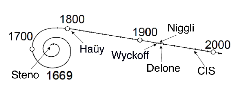
Figure 1: Some key dates in the history of modern crystallography

With the creation of the 1978 version of the Chemical Information System (CIS) [bernstein1979nih], building on the earlier CIS [feldmann1972application] which lacked cell search capabilities, online computerized retrieval systems become available for searching on ranges of unit cell parameters from the Cambridge Structural Database (CSD) [kennard1977computer]. From a few tens of thousands in 1979, the community has progressed to collection of several hundreds of thousands of sets of unit cell parameters, with approximately one million in the CSD by 2019 [taylor2019million] alone. When placed in a common SAUC database (see below), the number of cells in the Protein Data Bank and the Crystallographic Open Database total more than 600,000 entries as of summer 2022. Below, we discuss algorithms for robust searching on ranges of unit cell parameters. The need for ranges can be due to uncertainty of measurements, misidentified symmetry classes, variable composition, and searches for related materials.

There have been multiple databases that allow searching on the values of unit cell parameters, including:

• Chemical Information System (CIS) (1978 version), transferred to private management in 1984 [kadec1985transfer].

• Protein Data Bank, Rutgers Univ. [Bernstein1977] [Berman2000].

• Cambridge Structural Database. The WebCSD [hayward2019cambridge] cell search uses the [hayward2019cambridge] version of $\bf{G^{6}}$.

• American Mineralogist Crystal Structure Database [downs2003american].

• Crystal Lattice Structures. U.S. Naval Research Laboratory, now in the AFLOW library of crytallographic prototypes [mehl2017aflow].

• Crystallographic Database for Minerals and Their Structural Analogues, Russian Foundation of Basic Research [chichagov2001mincryst].

• ICSD Web: the Inorganic Crystal Structure Database, FIZ Karlsruhe [ruhl2019inorganic].

• Crystallography Open Database, University of Cambridge [gravzulis2012crystallography]

• SAUC (Search of Alternate Unit Cells), [McGill2014]

Various paradigms are used by different databases, sometimes only simple ranges on unit cell edge length. SAUC uses the methods described herein.

2 Introduction

Crystallographers, in general, seem convinced that unit cells are simple; after all, we learn about them on the first day of studying crystallography.

Likewise, lattices are considered to be simple. Of course there are complications, such as space groups, but the concept of the simple lattice is felt to be almost as simple as unit cells.

Stumbling blocks arise when the need to compare various unit cells is included in the tasks. For example, if the variations are due to temperature changes or site substitutions, it is not uncommon for the variations to be largely confined to a single parameter, such as one unit cell axial length.

A different issue arises with the need to compare the unit cells of an arbitrary group of materials. For instance, one might want to search in a database of all known materials. In those cases, more sophisticated tools are needed.

What modern problems require comparing arbitrary groups of cells?

• database searches (approximately a million unit cells are known)

• clustering for serial crystallography (thousands to hundreds of thousands of diffraction images in a single study)

• finding candidate materials for solving protein crystal structures [nanao2022id23]

• searches for minerals or alloys (both of which may have large compositional variation)

• Bravais lattice determination

• Studies in epitaxy [yang2014unit]

3 Techniques used to measure lattices

Several techniques other than common linear algebra methods will be used in measuring distances between unit cells.

• Metric vector spaces, see Section 5

• Simple topology, see Section 6

• “Fundamental region” (also called “fundamental unit”), see Section 9.1

• Unit cell reduction, see Section 9.6

• Projectors, see Appendix B

4 Unit cell parameters

If we are to measure the distance between two lattices, we will need to have a space where the measure can be performed. The conventional representation of a unit cell is the “unit cell parameters”, a, b, c, $\alpha$, $\beta$, $\gamma$. Mathematically, this is a point in $\bf{R^{3}\times R^{3}}$. That is the product of two different spaces; a point in one is not necessarily a point in the other; worse in this case is the fact that a point in the length space means nothing in the angle space. It is still possible to define a distance, but that would require inventing a unit that mixes the units of the length space and the angle space.

5 Spaces

In order to measure a meaningful distance between two objects, the objects need to be placed in a ”metric space”. For crystallographic unit cells, this will often be a vector space amenable to the tools and techniques of linear algebra, at least locally. Because six free parameters are needed to define a unit cell, the space will need to be at least six-dimensional. Depending on other criteria, more dimensions may be needed; gluing the edges of a manifold generates the need for more dimensions.

6 A digression on topology

One aspect of topology is the study of objects and the relationships of their edges, which can be “glued” together to make new objects and disclose new relationships among the parts. Here we look at a simple example that demonstrates some of the issues that arise in measuring distances between lattices.

6.1 Create a simple, 1D unit cell

Figure 2: This is just an empty single unit cell.

6.2 Put two atoms into the unit cell

Here we put atoms at the ends of the cell so that they will be close to their counterparts in the adjacent cell.

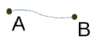
Figure 3: Put an atom at or near each of two boundaries of the unit cell

6.3 Connect the unit cell with its neighbors

Here we see that the “correct” distance between A and B is quite small compared to the distance within the fundamental cell.

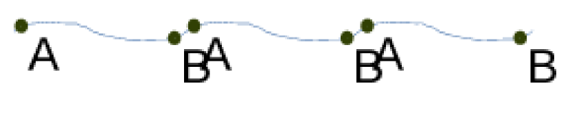
Figure 4: Here we show just the nearest neighbor cells

6.4 Another choice: wrap around into a loop

A technique based in topology is to wrap one edge of a cell through a higher dimensional space to join another edge of the cell to make a loop. Doing this can make the problem seem simpler, since there is only one cell to be considered. However, the problem of distance calculation has not been simplified. Now the distance has to be measured in both directions around the loop, and the shorter distance reported. This process of joining is termed “gluing”. In addition, the distance must be measured within the curved surface.

Gluing two edges of the one-dimensional cell turns the cell into a circle, making the problem two dimensional. If we had started with a two-dimensional cell, then gluing opposite pairs of edges could be used to make a three-dimensional torus. In either case, the dimensionality of the system would be increased by one.

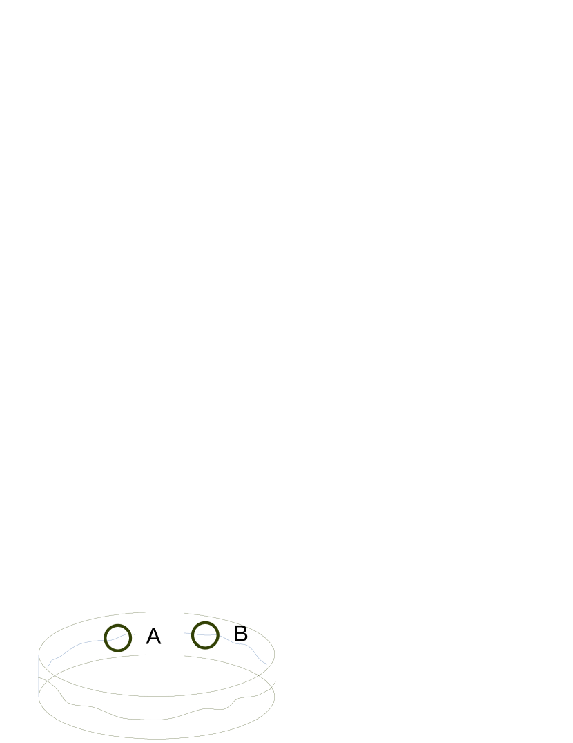
Figure 5:

6.5 Or you could twist the loop to make a Möbius strip

Consider the above case where the cell was on a 2-D surface. Instead of simply joining the ends, we can twist the loop before we glue the ends together, making a Möbius strip.

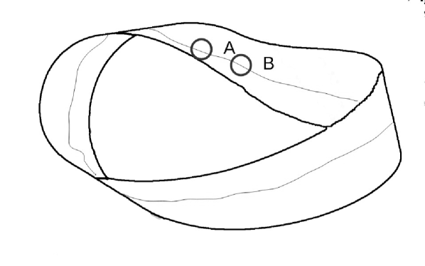
Figure 6: Twisting before joining makes a Möbius strip

6.6 Summary of the properties on joining

One aspect of gluing is that the dimensionality increases. The issue of measuring distances also become more complex. With added dimensions, the directions in which to look for shortest paths may increase. Similarly the glued boundaries themselves add to the cases to be considered in looking for shortest paths.

7 Spaces, continued

In this paper, we use several spaces to represent unit cells. Other choices of spaces are possible, but this set will suffice for the current topics.

• Lengths in Ångstroms and angles in degrees, a space of $R^{3}\times R^{3}$). Although the presentation of unit cell parameters as edge lengths and interaxial angles is familiar, it does not present an obvious metric (see Section 4). A possible alternative would be to treat each length and angle pair as a point in polar coordinates. This unexplored variation makes use of the association of each axis with its related angle, e.g. a and $\alpha$ (see appendix D).

• $\bf{G^{6}}$ (Niggli space) (see appendix E)

• $\bf{S^{6}}$ (Delone space) (see appendix F)

• $\bf{C^{3}}$ (see appendix G)

For future reference, we are in the process of extending this list by consideration of a seven-dimensional space of Wigner-Seitz cells [Bernstein2023].

8 Fundamental region

In working with a space in which there are multiple symmetry-related occurrences of items of interest (atoms, molecules, or, in this case, unit cells), it is conventional to choose a fundamental region [enwiki:1028832752]. In a two-dimensional graph, it would often be chosen as the all-plus quadrant. In crystallography, it might be a unit cell, a particular asymmetric unit of a crystal, or even a molecule.

The conventional fundamental unit for Niggli space is the region of $\bf{G^{6}}$ that contains the Niggli-reduced unit cells. This choice has the disadvantage that the fundamental region is non-convex, and the boundaries are complex [Andrews2014].

For Delone space, the fundamental unit is conventionally chosen as the all-negative orthant of $\bf{S^{6}}$, which contains all reduced cells. In this orthant, all non-boundary points (that is, those having no zero scalars) correspond to a computable unit cell. All points with one or two zero scalars also correspond to valid unit cells. Boundaries that have four, five, or six zeros have no valid cells. For three zeros, there are valid cells except for those points with a prototype of $s_{1},s_{2},s_{3},0,0,0$ [Andrews2019b].

The all-negative orthant (excluding the boundaries) is an “open” manifold in topological terms; all points there correspond to exactly one lattice. The fact that certain boundaries do not correspond to valid unit cells complicates certain aspects of its topology.

9 Measuring

Measuring the distance between two lattices comes down to finding a geodesic between them, i.e. a minimal length path between them obeying the rules for points in the space. We first give a simple example of points in a 2-D manifold, which demonstrates some of the complexity of treating lattices.

9.1 Step 1, fundamental unit

The obvious step to find the shortest distance between two lattices is to simply compute the Euclidean distance between them in the fundamental unit. That distance might not be the shortest that can be found, but no geodesic could be longer. It makes a useful starting point. Call this distance $d_{0}$.

9.2 Boundaries

The next step is to consider the boundaries of the fundamental unit. If there is no boundary with a shorter distance to either of the lattices than $d_{0}$, then $d_{0}$ is the required minimum.

If either lattice does have a boundary closer to it than $d_{0}$, call the shortest distance from the first lattice to any boundary $d_{1}$ and the shortest distance from the second lattice to any boundary $d_{2}$. If $d_{1}+d_{2}>d_{0}$ then $d_{0}$ is still the required minimum and we are done. It is only when both lattices are closer than this to some boundaries that we need to engage in a more complex search for geodesics.

As a simple example of treating boundaries, consider a plane with a single symmetry element, two-dimensional point group 4.

We choose the lower left quadrant to be the fundamental unit. This is an arbitrary choice.

Now put a single atom, A, in the plane, and apply the 4-fold operation.

Now let us consider what happens if we place three atoms, A, B, and C in the fundamental unit.

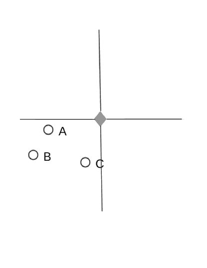
Figure 7:

It is clear that within the fundamental unit, ignoring all symmetry transforms and considering B and C, B is the atom closer to A. Draw a circle centered on A that touches B. We see that the circle crosses the boundary and a portion is outside of the fundamental unit. Any atom that is within that region outside the fundamental unit must be examined to see if it contains an atom.

Applying the 4-fold operation to the shaded segment, we see that the atom C (in the fundamental unit) is closer to A than B is to A.

The next part of the problem is how to compute the actual distance from A to C. The obvious answer is to apply the 4-fold symmetry operation either to A or to C and measure the Euclidean distance. We will see in the next section that such simplistic solutions are not sufficient for lattices.

9.3 Spaces for measuring

From this point on, only two spaces will be used for specific examples, $\bf{S^{6}}$, the space of Selling scalars as six real vector components, $(P,Q,R,S,T,U)$ = ($\mathbf{b}\cdot\mathbf{c}$, $\mathbf{a}\cdot\mathbf{c}$, $\mathbf{a}\cdot\mathbf{b}$, $\mathbf{a}\cdot\mathbf{d}$, $\mathbf{b}\cdot\mathbf{d}$, $\mathbf{c}\cdot\mathbf{d}$) where $\mathbf{d}=-\mathbf{a}-\mathbf{b}-\mathbf{c}$, and $\bf{C^{3}}$, the same scalars as $\bf{S^{6}}$, but used as the real and imaginary parts of three complex vector components, $(P+iS,Q+iT,R+iU)$, with each complex number written as a column two-vector. See sections F and G in the appendices. $\bf{C^{3}}$ is simply an alter ego of $\bf{S^{6}}$, but some operations are simpler to describe in $\bf{C^{3}}$. The reason for limiting our consideration to these two spaces is their simplicity compared to other spaces. As stated above, the fundamental unit of $\bf{S^{6}}$ is a simply-connected, convex manifold, with only a few excluded regions (multiple zeros).

For any given lattice there are infinitely many choices of cells from that lattice that can be used to represent it. The point of reduction is to unambiguously choose a single one of those choices of cells. In the absence of experimental error that is what, for example, Niggli reduction does. In the presence of experimental error things are not so simple and any of several equally valid, but very different, unit cells may end up being chosen to represent the same lattice [Gruber1973] [McGill2014].

9.4 Reflections, a simple example

Reflections in $\bf{S^{6}}$ were defined in Andrews2019b. They are the operations that create isometric copies of a lattice, always within the fundamental unit. When comparing two lattices, it is necessary to examine the distances from a reduced cell in one lattice to each of the reflections of another reduced cell in the other lattice.

Returning to Figure 7 (where the distance to objects outside the fundamental unit were considered), consider instead the two-dimensional point group 4mm. Figure 8 shows a subset of the reflections of the basic set of three points. Immediately, it is clear that in this case, the distance between two copies of point A is the shortest.

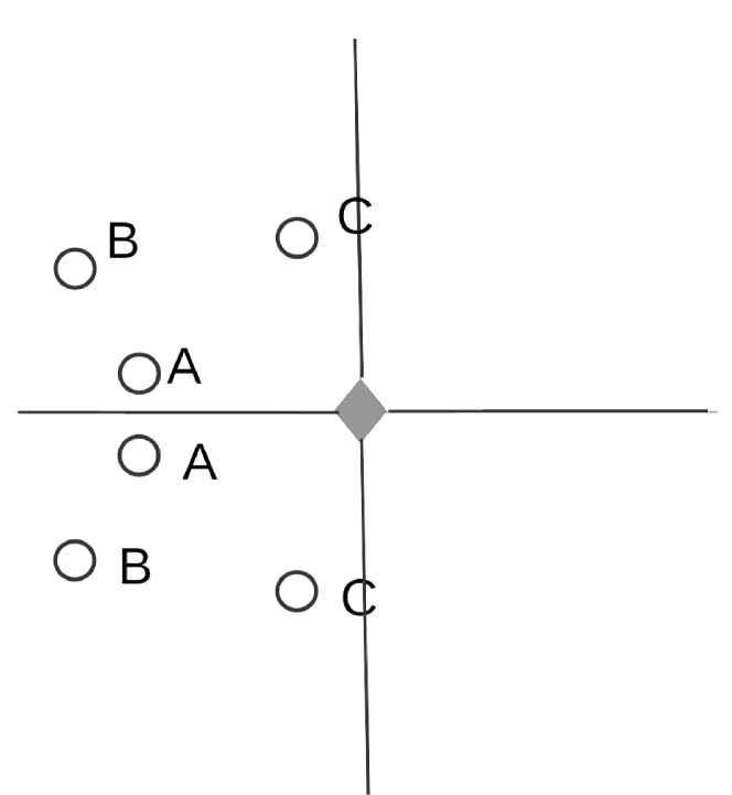
Figure 8: Recreating the above example, but with point group 4mm.

9.5 Reflections in $\bf{S^{6}}$ and $\bf{C^{3}}$

“Reflections” were defined byAndrews2019b as the 24 operations that create different, reduced versions of a reduced cell in $\bf{S^{6}}$ and $\bf{C^{3}}$ (isometric copies). By this definition, the 4-fold operation and the mirrors in point group 4mm (see Figure 8) are reflections.

An important difference between Niggli space and Delone space is that Niggli space has the vector scalars sorted by somewhat complex rules. $\bf{S^{6}}$ (that is, Delone space) being unsorted results in there being multiple points in the fundamental unit for each lattice. In general, there are 24 reflections, but equal scalars and zero scalars can lead to degeneracies.

The reflections are simpler to describe in $\bf{C^{3}}$, but, of course, the same ones exist in $\bf{S^{6}}$. Here we use the $\bf{C^{3}}$ vectors: $c_{1}$, $c_{2}$, and $c_{3}$, see Appendix G.

First there are the three interchanges of scalars: $c_{1}\Longleftrightarrow c_{2}$, $c_{1}\Longleftrightarrow c_{3}$, and $c_{2}\Longleftrightarrow c_{3}$.

There are also reflections that interchange elements within scalars.

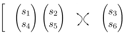
Figure 9: Example of interchanging real and imaginary scalars for the case of reduction of scalar $s_{1}$.

And finally each pair of the reflections needs to be combined giving a total of 24.

9.6 Reduction

The objective of reduction in $\bf{S^{6}}$ (and in $\bf{C^{3}}$) is to make each Selling scalar less than or equal to zero. If any scalar is greater than zero, there are two stages to a reduction step. First, a vector is composed and added to the vector being reduced. Then two scalars are interchanged as shown in Figure 10.

While any scalar can be the one to be reduced, this figure shows the operations for $s_{1}$.

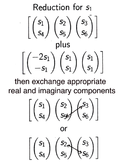
Figure 10: Steps for reduction in $\bf{C^{3}}$

9.7 Boundary transformations

The transformations for crossing boundaries of the fundamental unit are the reduction operations.

The section on fundamental regions (see Section 8) shows the problem of points outside the fundamental unit and how boundary transformations were applied there. The boundary transformations for lattices are more complex than those of space groups.

1. The boundaries must be identified.

2. The transformations at the boundaries in $\bf{G^{6}}$ and $\bf{S^{6}}$ are not isometric, meaning that they do not preserve distance measure.

3. For a particular boundary, there may be more than one allowed transformation available.

4. Applying a transformation to a point near a boundary may generate a new point that is near another boundary, requiring further searching.

5. A point that is in the fundamental unit but close to a boundary might need to be transformed in order to find other nearby points.

6. All measurements must be done in the metric of the fundamental unit. A corollary is that when two points are being treated, one must be held fixed and within the fundamental unit while the possible boundary transformations and reflections of the other are treated.

7. If a point is near more than one boundary, then there are multiple transformations and reflections to consider.

The fundamental unit in $\bf{S^{6}}$ is the all-negative orthant. The boundaries are all where one (or more) of the scalars equals zero. Two points that are close together and have a corresponding scalar that is positive in one and negative in the other may have representations in the fundamental unit that are far apart.

In Figure 11a, the two points with $\gamma=89.8^{\circ}$ and $\gamma=90^{\circ}$ are far apart.

Figure 11b demonstrates a further complexity. Because the angles $\alpha$ and $\beta$ were chosen to be $90^{\circ}$, all points in Figure 11a sit on two boundaries ($beta$=$90^{\circ}$ and $\gamma$=$90^{\circ}$, $s_{4}$=$0$ and $s_{5}$=$0$). Perturbing those boundary points may cause them to be within the fundamental unit, but, on the other hand, may cause them to be outside and thus be far from the neighboring points (after reduction). All the gray lines correspond to members of lattice pairs that are close together but are far apart in the fundamental unit (that is, Delone-reduced).

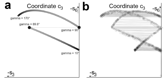
Figure 11: In both figures (a) and (b), a series of points has been generated in $\bf{S^{6}}$. The basic cell is a=10, b=10, c=10, $\alpha=90^{\circ}$, $\beta=90^{\circ}$, and $\gamma$ ranges sequentially from $10^{\circ}$ to $170^{\circ}$, in $0.2^{\circ}$ increments. Each cell was Delone-reduced. Each was then placed in the $\bf{C^{3}}$ asymmetric unit [Andrews2019b]. Then, in sequence from the first cell, for the succeeding cell, all 24 reflections of the succeeding cell were examined, and the reflection that is closest to the first cell chosen. Calculation then proceeds to the next pair (where the new first is the second chosen in the previous step). A line (shown in gray) was drawn between each successive pair of points. The individual points are shown as circles.    This figure shows the points converted to $\bf{C^{3}}$, and the c3 coordinate is displayed. In figure (a) on the left the points are generated as described. The gray connection lines, except for the one connection $\gamma=90^{\circ}$ to $\gamma=89.8^{\circ}$, are hidden by the circles. That single long line represents a case when distance measured in the fundamental unit is quite long, although the originally generated points are quite close together. In figure (b) on the right, initially, three copies of each point were generated, and all points were perturbed by 1% in a random direction orthogonal to the generated vector (point). Then (in the order of generation), the above sequencing was performed.    Because the basic structure of the point generation requires that all points be on multiple boundaries, there are many cases where the distances in the fundamental unit are long. Every gray line is a case where the simple Euclidean distance in the fundamental unit is long, but the generated points are close together.

As seen in Figure 11, points that are a small distance apart may be far apart in the fundamental unit. As an example, we choose a primitive cubic unit cell, $\bf{S^{6}}$ vector $\begin{bmatrix}{0,0,0,10,10,10}\end{bmatrix}$. In Figure 12, 1000 copies have all been perturbed by 1% in a direction orthogonal to that vector.

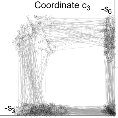
Figure 12: 1000 copies of $\bf{S^{6}}$ vector $\begin{bmatrix}{0,0,0,10,10,10}\end{bmatrix}$ were perturbed by 1% orthogonal to the vector. As in Figure 11, for each pair of points, the second point was chosen to be the reflection that is closest to the first point. The choice of reflection pairs was done by treating the list of generated points as a sequence. Long lines indicate pairs that are far apart within the fundamental unit.

10 Boundaries (and reduction) in $\bf{S^{6}}$ and $\bf{C^{3}}$

10.1 Multiple boundaries

If a point is near two boundaries, all the cases for each boundary need to be considered (recall that in $\bf{S^{6}}$ there are four possible boundary transformations at each of the six boundaries). In addition, applying the transformations of one of the boundaries and then those of the second is necessary. That means that there are 16 possible results. Further still, the case of applying them in the other order must be considered (resulting in another 16 cases).

For the case of being near three boundaries, similar complexity to the case for two boundaries must be considered: all single boundaries, all boundary pairs (in both orders) and all triples (in all possible orders).

10.2 Repeated boundaries

In some cases, applying a boundary transformation results in one of the modified scalars being near a boundary that it was not near before. Such a case requires that the new neighbor boundary also be considered.

10.3 Iteration

Much of the complexity of determining the shortest distance between two lattices is due to the need to repeat steps of reduction and reflection. Among the places in the process where this becomes necessary is when a reduction step creates a new point that is near a boundary.

10.4 Measuring lattice distances in $\bf{S^{6}}$

Figure 13: In space $\bf{S^{6}}$, choose two axes. The operations shown will be a cartoon of the operations in six-space.

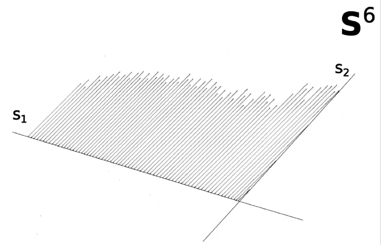
Figure 14: Define a fundamental unit (all non-positive region).

Figure 15: Put in a unit cell (a point in $\bf{S^{6}}$).

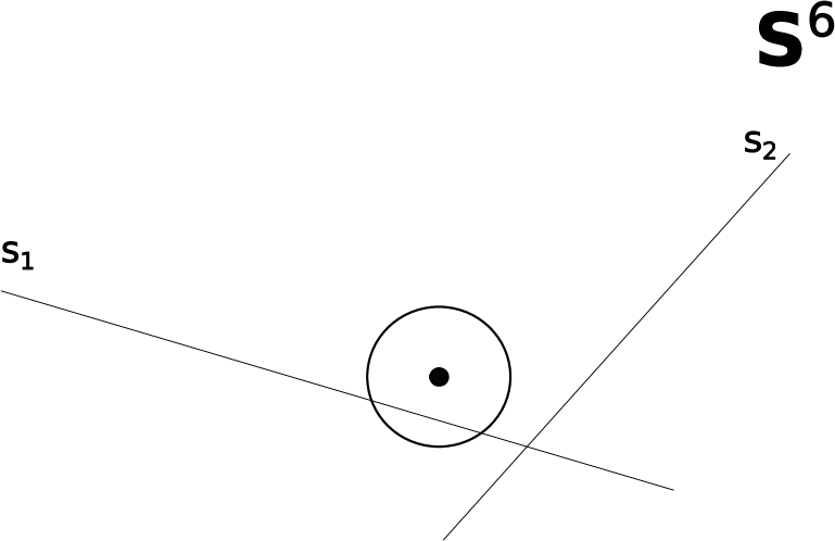
Figure 16: Define a search radius. In this case, it crosses a boundary and a region is outside the fundamental unit. Cells there are not reduced.

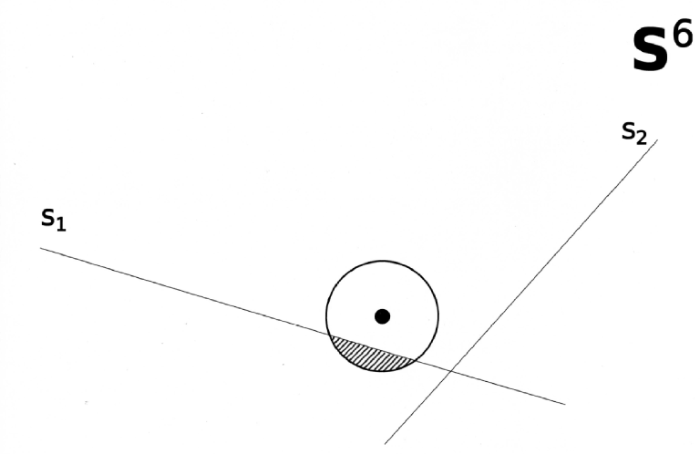
Figure 17: The non-reduced region is marked in crosshatch.

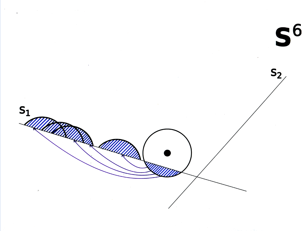
Figure 18: Unlike in the 4-fold example, there are multiple (up to 4) places to go. A further complication is that the transformations at the boundaries do not preserve distances. Distances must be measured in the frame of the fundamental unit.

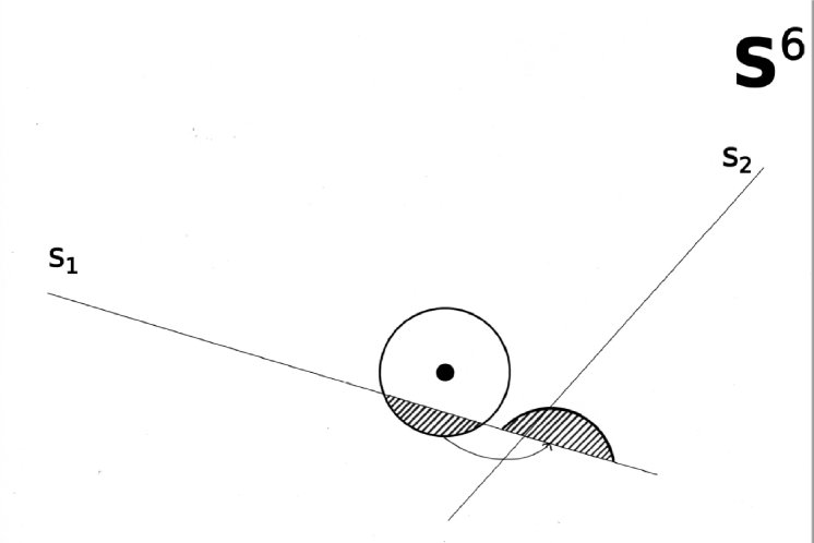
Figure 19: Sometimes, in the process, another boundary is crossed. Then further iterations may be required.

The distance between two lattices is determined by first computing $d_{0}$, the minimum of all the Euclidean distances between reflections of those two points within the fundamental unit. If either lattice is closer to any boundary than $d_{0}$, then we need to iterate through all possible paths that may cross a boundary.

If the second point is near a boundary, then the four transforms for that boundary are applied. We need to compute the tunneled distances. If the generated points are not near another boundary, then we are done. If they are near a new boundary, then we need to iteratively apply the boundary transforms.

1. Reduce both unit cells.

2. Choose one point (“first point”) to be the fixed point, and the other (“second point”) to be the one to which transformations are applied.

3. Compute $d_{0}$, the minimum of all the Euclidean distances between the first point and all reflections of the second point (the reflected points are all within the fundamental unit).

4. Compute $d_{1}$, the minimum of all the Euclidean distances between the first point and all boundaries.

5. Compute $d_{2}$, the minimum of all the Euclidean distances between the second point and all boundaries.

6. If $d_{1}+d_{2}<d_{0}$, then there may be a path between some reflection of the first point and some reflection of the second point that is shorter than $d_{0}$ that crosses a boundary. It is sufficient to explore possibly shorter paths by leaving the first point fixed and only considering reflections of the second point. For each boundary to be considered there are at most four possible paths from whichever of the two points is close enough to that boundary to satisfy $d_{1}+d_{2}<d_{0}$. For such a case we need to iterate through all four possible paths that may cross the boundary.

7. If the second point is near two or three boundaries, then each boundary needs to be treated by itself. Then all pairs (and all triples) in all permuted orders must be transformed through the boundaries by all four paths of each boundary. For a given $\bf{S^{6}}$ boundary there are four possible boundary transforms to consider which may take a reflection of the second point outside of the fundamental unit (see Figure 18).

8. If the points produced in the above steps are near new boundaries, then the above steps need to be iterated using the new points.

9. N.B., the distance must be measured in the metric of the fundamental unit; see section 10.5.

In the above discussion of gluing in topology, mention was made of the increase in dimensions as edges are glued and more if there are twists. Here, the boundary transformation operations interchange two scalars, and that is a twist operation. Counting up the gluings and twists leads to the conclusion that the required dimension of the space in which to embed the glued manifold is quite high; immediately, we understand that there are potentially going to be many paths to examine.

10.5 Measuring with the metric of the fundamental unit

The problem that arises in computing distances between lattices is that it is necessary to transform points to be outside the fundamental unit. The boundary transformations are not isometric; distance measure is not preserved on crossing out of the fundamental unit. Here we describe how to create a measure for those points that is isometric.

If the second point of a measurement is near a boundary, then project the point onto the boundary (the dashed arrow in Figure 20) and extend the line segment from the second point to the boundary to twice the length creating a transformed point creating an artificial mirror point. The “Tunneled Mirrored Boundaries” distance is found by locating the crossing point on the boundary where the line from the first point to the artificial mirror point crosses the boundary and then finding the four boundary transforms of the crossing point. Applying a boundary transform to the crossing point provides an alternate boundary point to be used for a broken path (first point to crossing point point – equivalent to boundary-mapped crossing point, followed by mapped crossing point to second point). This broken path is sometimes shorter than the direct $d_{0}$ path and is entirely in the fundamental unit. If two boundaries are close, then similar actions on both lattice points are needed.

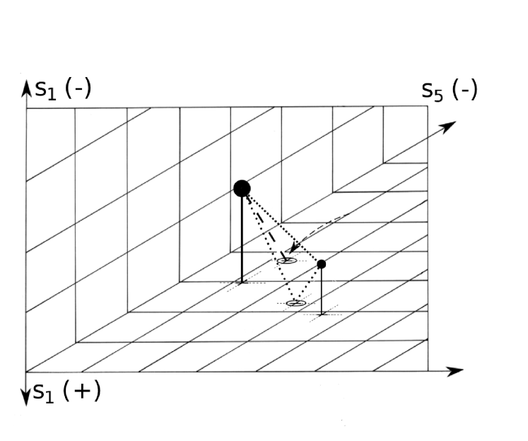
Figure 20: Tunneled Mirrored Boundary

10.6 Algorithm

For finding the shortest distance between two reduced lattices, the first step is to compute the simple Euclidean distance between them. Each lattice is considered as a point in a space of six or more dimensions with a metric derived from the cell reduction rules for that space.

If the original second point is near one (or more) boundaries, then the the boundary searches (above) are performed.

If new near-boundary-contacts are detected, then the same kind of searches is performed.

Distances must be measured in the metric of the fundamental unit not in the metric of any region outside the fundamental unit.

10.7 Nearest neighbors, the “Post Office Problem”

Up to this point, the discussion has targeted finding the shortest distance between two lattices. Sometimes, the problem is to find the collection of points that are near a particular probe. One important use is for creating and for searching within databases of crystals. Known as the nearest neighbor problem, it is also known as the post-office problem [Andrews2001], and [Andrews2016]. (see Appendix C.)

11 Determining Bravais lattice types

11.1 Notation

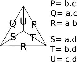
Figure 21: Bravais organized the scalars into a “tetrahedron”[Delaunay1932].

The International Tables for Crystallography define this assignment of the scalars (PQRSTU) in the tetrahedron [donnay1953international]. Other authors used alternative assignments.

As $\bf{S^{6}}$: s = $\begin{pmatrix}{P,Q,R,S,T,U}\end{pmatrix}$
= $\begin{pmatrix}{s_{1},s_{2},s_{3},s_{4},s_{5},s_{6}}\end{pmatrix}$.

As $\bf{C^{3}}$: $\begin{bmatrix}\begin{pmatrix}P\\ S\end{pmatrix}\begin{pmatrix}Q\\ T\end{pmatrix}\begin{pmatrix}R\\ U\end{pmatrix}\end{bmatrix}$

11.2 Bravais lattice types in $\bf{S^{6}}$

Delaunay1932 and Delone1975 produced a table classifying the reduced forms of the Bravais types as 24 cases. Figure 22 shows the same classification (the letter codes for crystal systems have been changed to modern notation. For some types, revised names have been given to Delone’s types where a cell included two types (for example, Delone’s “M1” is split into “M1A” and “M1B”). In Figure 22, the Bravais type is listed, and the restrictions on $\bf{S^{6}}$ scalars is shown graphically as the Bravais tetrahedron and listed as the lattice character.

Figure 23 describes the contents of each table entry in Figure 22.

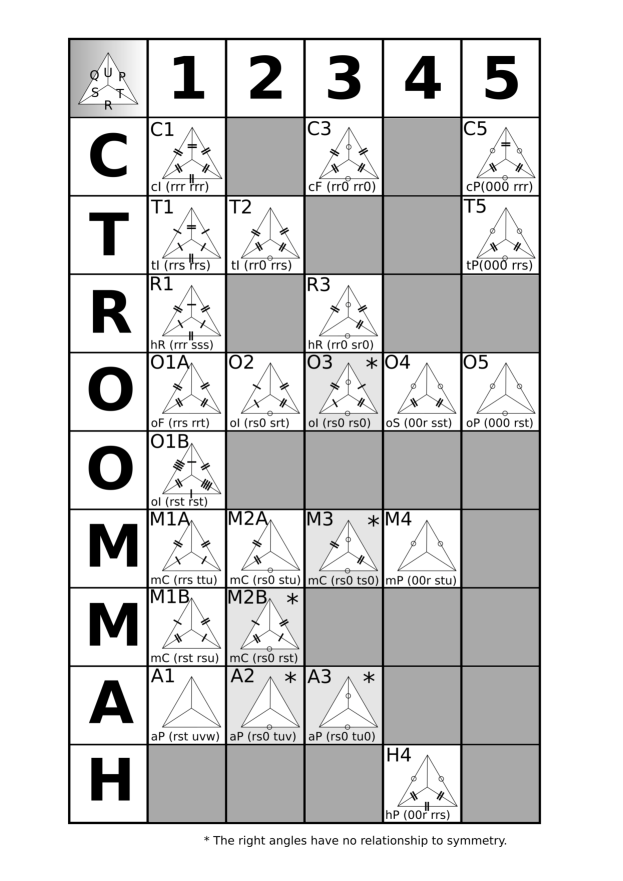
Figure 22: The table of Delaunay1932 describing the 24 Bravais types in $\bf{S^{6}}$. It has been redone removing the images of the Dirichlet cells, the non-reduced cells, and adding the “lattice character”, which describes the linear manifold of each type. The crystal family types have been renamed to modern usage: Q changed to T for tetrahedral, K changed to C for cubic, and T changed to A for anorthic. Where Delone in some places included two types in one table cell, they have been split into two (for example: “M1” is split into “M1A” and “M1B”. Note that five types (O3, M3, M2B, A2, and A3) are not normal crystallographic types. They are boundary types, and they have fewer free parameters than the generic type requires. For instance, O3 (character: rs0 rs0) has only two free parameters (r and s), whereas an ordinary orthorhombic type requires three variables.

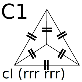
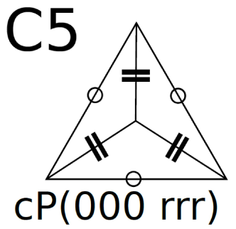
Figure 23: Explaining the information in Figure 22; it includes the name of the Delone type (e.g.: C1),the Bravais type (e.g.: cI for body-centered cubic), and the lattice character that describes the linear manifold of each Delone type (e.g.: 000 rrr). The markings on the tetrahedra describe the restriction on the $\bf{S^{6}}$ scalars; they encode the same information that is in the lattice character. A zero (circle) means that the value of that scalar is zero, several with the same lines means they are constrained to be equal; in Figure 23, they are a pair of double line hatches.

11.3 How to determine Bravais lattice types

First, the projectors for each type are necessary. There are two ways to determine the Bravais lattice type.

1. The program BGAOL uses methods essentially the same as those used for distance calculations. For a given input unit cell, the reflections and boundary transformations are applied. The original cell and each of the transformed cells, is projected onto each of the manifolds of the lattice types (24 in the cases of $\bf{S^{6}}$). The distance from the probe cell to the projected cell is the agreement factor. For each lattice type, the cell with the shortest distance is reported.

2. The program SELLA [andrews2022unnecessarily] starts from vectors representing each of the lattice types and transforms them using the reflections and first layer boundary transformations. (In the case of multiple boundaries, all combinations must be used as in distance calculations). Then the distance from the reduced probe to each of the transformed manifolds of each type is computed. The shortest distance to one of the transformed manifolds is reported. If needed, the inverse reduction of the input (unreduced) unit cell can be applied to the best projected cell to get the best approximation of the input.

11.4 What do you need to compute distances?

• Reflections

  • $\bf{G^{6}}$ [Andrews2014]

  • $\bf{S^{6}}$ [Andrews2019b]

• Boundary transforms

  • $\bf{G^{6}}$ [Andrews2014]

  • $\bf{S^{6}}$ [Andrews2019a] (only two, following Delone, but reflections generate a total of 4)

• Bravais lattice projectors

  • $\bf{G^{6}}$ [paciorek1992projection]

  • $\bf{S^{6}}$ [andrews2022generating]

• Lattice characters

  • $\bf{G^{6}}$ [Andrews2014]

  • $\bf{S^{6}}$ see Section 11.5

11.5 $\bf{S^{6}}$ Bravais lattice characters

Each Bravais type defined by Delaunay1932 corresponds to a linear manifold in $\bf{S^{6}}$. The definitions of each type were described by markings on the elements of the tetrahedra for each type in Figure 22. For implementation in software, it is more convenient to use the “lattice characters” that describe the restrictions.

type Bravais type & character C1 cI (rrr rrr) C3 cF (rr0 rr0) C5 cP (000 rrr) T1 tI (rrs rrs) T2 tI (rr0 rrs) T5 tP (000 rrs) R1 hR (rrr sss) R3 hR (rr0 sr0) H4 hP (00r rrs) type Bravais type & character O1A oF (rrs rrt) O1B oI (rst rst) O2 oI (rs0 srt) O3 oI (rs0 rs0) * O4 oS (00r sst) O5 oP (000 rst) O4 oS (00r sst) O5 oP (000 rst) type Bravais type & character M1B mC (rst rsu) M2A mC (rs0 stu) M2B mC (rs0 rst) * M3 mC (rs0 ts0) * M4 mP (00r stu) A1 aP (rst uvw) A2 aP (rs0 tuv) * A3 aP (rs0 tu0) * M1A mC (rrs ttu)

* cases of non-crystallographic $\bf{S^{6}}$ scalars ($90^{\circ}$ angles)

11.6 Lattice Matching

A common problem in crystallography is to provide a list of the unit cells of several (or many) crystals so that they can be visually compared, making it easier to identify meaningful clusters of crystals of related morphology. Data collections of unit cells have been created based on similarity of morphology (for example, see Donnay1963. In recent years, the clustering of unit cells from the myriad of images in serial crystallography has been increasingly important.

For each transformed vector, one must store the transformation that will bring it back to the original presentation.

Start with a collection of experimental unit cells. From among them, we select or create the “reference” cell; that is the one to which all the rest will be matched as closely as possible.

We transform the reference cell by many operations in the course of exploring alternative lattice representations. For each newly generated lattice representation,we accumulate the transformations needed to convert back to the original reference cell. All of these operations are be performed in $\bf{S^{6}}$.

Only accumulate transformations that have not already been found (to avoid duplication).

Next all the accumulated, transformed representations of the reference cell must be scaled to a common length and the saved transformations inverted which allows one to return a vector to its original presentation. For improved searching in the final step, it is convenient to store the the vectors in a nearest neighbor search application such as NearTree [Andrews2016]. This ends the preprocessing of the reference lattice.

To match a probe lattice to the reference cell, first the probe lattice should be Selling reduced. Then the nearest point of the collection of transformed lattice points to the reduced probe is found. The stored transform of the nearest reference is applied to the reduced probe to generate the best approximation.

As an example, consider the case of krait toxin phospholipase A2 [LeTrong2007]. Table 1 shows 6 reported forms from the Protein Data Bank. The lattice type and unit cell parameters are as initially reported.

Table 2 shows the same data in the same order after lattice matching to the first entry (1DPY). The immediate conclusion is that the crystals are likely the same crystal form.

Table 1: Unit cells of phospholipase A2 from the Protein Data Bank.

PDB		a	b	c	$\alpha$	$\beta$	$\gamma$
1DPY	R	57.98	57.98	57.98	92.02	92.02	92.02
1FE5	R	57.98	57.98	57.98	92.02	92.02	92.02
1G0Z	H	80.36	80.36	99.44	90	90	120
1G2X	C	80.95	80.57	57.10	90	90.35	90
1U4J	H	80.36	80.36	99.44	90	90	120
2OSN	R	57.10	57.10	57.10	89.75	89.75	89.75

Table 2: The data of Table 1 matching a rhombohedral reference. The reference cell is marked in boldface.

PDB	a	b	c	$\alpha$	$\beta$	$\gamma$
1DPY	57.98	57.98	57.98	92.02	92.02	92.02
1FE5	57.98	57.98	57.98	92.02	92.02	92.02
1G0Z	57.02	57.02	57.02	90.39	90.39	89.61
1G2X	57.10	57.11	57.11	89.25	90.25	90.25
1U4J	57.02	57.02	57.02	90.39	90.39	89.61
2OSN	57.10	57.10	57.10	90.25	90.25	89.75

12 Various available programs

• SAUC: Search for related unit cells

• BGAOL: Determine likely cells of higher symmetry

• Follower: Compute distances between cells along a path

• LatticeMatching: Try to match a reference cell

• SELLA: Determine likely cells of higher symmetry

• various cmd programs–

  12.1 SAUC (Search of Alternative Unit Cells)

  SAUC is software plus an online database of the Protein Data Bank unit cells and the Crystallographic Open Database unit cells.
  "https://iterate.sourceforge.net/sauc/"
  SAUC provides searching for several alternate distance measures, including $\bf{S^{6}}$ and $\bf{G^{6}}$. Searching by nearest neighbor allows specifying various criteria, such as percent range, nearest neighbors, or within a sphere of specified radius.
  

  A useful example is that of krait toxin phospholipase A2 [LeTrong2007].

  Starting from PDB entry 1u4j with cell parameters: (80.36, 80.36, 99.44, 90, 90, 120) in space group R3 with a distance cutoff of 3.5Å using the $\bf{G^{6}}$ metric, four structures of phospholipase A2 are found.

  PDB code G6 distance protein name 1u4j 0.0 Phospholipase A2 isoform 2 1g0z 0.0 Phospholipase A2 1g2x 0.9 Phospholipase A2 2osn 0.9 Phospholipase A2 isoform 3

  12.2 BGAOL - Bravais General Analysis of Lattices

  BGAOL is an online program for seeking possible Bravais lattice types for a given unit cell.

  https://iterate.sourceforge.net/bgaol/
  

  Consider 1,8-terpin [Mighell2001] with unit cell 10.912(2), 22.79(4), 10.705(2), 90, 120.64, 90.

  The BGAOL results (only the best 4, which are also 1,8-terpins) are:

  lattice	distance		unit	cell
  oF	0.025	18.419	22.790	10.912	90	90	90
  mC	0.025	10.912	18.419	12.634	90	115.585	90
  mI	0.000	10.704	22.790	10.705	90	118.713	90
  mI	0.018	14.652	10.912	14.651	90	102.109	90

  The unit cells reported in Table 12.2 are then matched to the lattice type in column 1. If the discovered lattice type is monoclinic (in this case mI), then the unit cell is projected into the manifold of the discovered type.

  A web site on which searches may be done is located at http://iterate.sourceforge.net/bgaol/.

  13 Summary

  Unit cells are used to represent crystallographic lattices. Calculations measuring the differences between unit cells are used to provide metrics for measuring meaningful distances between three-dimensional crystallographic lattices. This is a surprisingly complex and computationally demanding problem. We present a review of the current best practice using Delaunay-reduced unit cells in the six-dimensional real space of Selling scalar cells $\bf{S^{6}}$ and the equivalent three-dimensional complex space $\bf{C^{3}}$. The process is a simplified version of the process needed when working with the more complex six-dimensional real space of Niggli-reduced unit cells $\bf{G^{6}}$. Obtaining a distance begins with identification of the fundamental region in the space, continues with conversion to primitive cells and reduction, analysis of distances to the boundaries of the fundamental unit, and is completed by a comparison of direct paths to boundary-interrupted paths, looking for a path of minimal length.

  Appendix A Availability of code

  Code supporting this paper is available on github at http://github.com/duck20/LatticeRepLib.git and http://github.com/yayahjb/ncdist.git.

  Appendix B Projectors

  Orthogonal projectors onto linear subspaces can be calculated from any algebraic descriptor of that subspace that can provide a matrix $X$ with vectors that at least span that subspace. Redundant vectors can help to improve the accuracy of the calculation. If $A$ is the columnspace of $X$, then $P=A(A^{T}A)^{-1}A^{T}$ is a projector onto that linear subspace, and $PP=P$ and $P^{T}=P$.

  The application of a projector yields the least-squares best fit.

  

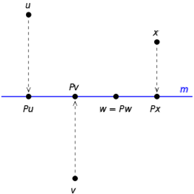
  Figure 24: Example of projectors: they are the operators that do orthogonal projection.

  Appendix C Nearest neighbor search

  Wikipedia has a useful description of nearest neighbor searching [enwiki:1103897119].

  Code for nearest neighbor searching using NearTree is available on GitHub at http://github.com/yayahjb/neartree.git. NearTree uses the algorithm of kalantari1983data with enhancements for other kinds of searches.

  Appendix D Polar coordinates

  Expressing unit cell parameters as edge lengths and angles does not lead to a easily interpreted metric: lengths and angles are not commensurate. An unexplored alternative is to express them in polar coordinates, which is equivalent to expressing them in complex coordinates.

  Delone pointed out that the “opposite” scalars form special pairs. The Bravais tetrahedron is the origin of his use of the term “opposite”. Another way to view this relationship is to organize the six scalars into three pairs, treating the first member of the each pair as the real component of a complex number and the second member of each pair as the imaginary component. Write the definition of an $\bf{S^{6}}$ vector $(s_{1},s_{2},s_{3},s_{4},s_{5},s_{6})$ in $\bf{C^{3}}$:
  

  $\begin{bmatrix}$ \begin{tabular}[]{ c c l c }$\begin{pmatrix}s_{1}\\ s_{4}\end{pmatrix}$ \par$\begin{pmatrix}s_{2}\\ s_{5}\end{pmatrix}$ \par$\begin{pmatrix}s_{3}\\ s_{6}\end{pmatrix}$\end{tabular} $\end{bmatrix}$
  
  

  Rewriting the definitions of the $\bf{S^{6}}$ scalars, we see that for each $\bf{C^{3}}$ scalar, the angle in the real position, is related to the edge vector used in the imaginary position. For instance for $c_{1}$, alpha is associated with $a$. For reflections, these associations are not changed.
  

  $\begin{bmatrix}$ \begin{tabular}[]{ c c l c }$\begin{pmatrix}\bf{b\cos{\alpha}~{}c}\\ \bf{a\cdot d}\end{pmatrix}$ \par$\begin{pmatrix}\bf{a\cos{\beta}~{}c}\\ \bf{b\cdot d}\end{pmatrix}$ \par$\begin{pmatrix}\bf{a\cos{\gamma}~{}b}\\ \bf{c\cdot d}\end{pmatrix}$\end{tabular} $\end{bmatrix}$
  

  The stability of the angle/edge length association implies that a potentially useful new coordinate system for describing unit cells might be $\begin{pmatrix}a,\alpha\end{pmatrix}$, $\begin{pmatrix}b,\beta\end{pmatrix}$, $\begin{pmatrix}c,\gamma\end{pmatrix}$.

  Appendix E The linear space $\bf{G^{6}}$ (Niggli space)

  Label the cell axes ${\textbf{a},\textbf{b},\textbf{c}}$. The scalars are ${{\bf\textbf{a}\cdot\textbf{a}}}$,  ${{\bf\textbf{b}\cdot\textbf{b}}}$,  ${{\bf\textbf{c}\cdot\textbf{c}}}$,   2${{\bf\textbf{b}\cdot\textbf{c}}}$,  2${{\bf\textbf{a}\cdot\textbf{c}}}$,  2${{\bf\textbf{b}\cdot\textbf{c}}}$ where, e.g., ${{\bf\textbf{b}\cdot\textbf{c}}}$ represents the dot product of the b and c axes. In order to organize these six quantities as a vector space in which one can compute simple Euclidean distances, we describe this set of scalars as a vector, g, with components, ${g}_{1},{g}_{2},{g}_{3},{g}_{4},{g}_{5},{g}_{6}$. [Andrews2014] It should be noted that the first three scalars of $\bf{G^{6}}$ are the diagonal elements of the metric tensor. The second three are the off-diagonal elements, doubled. One reason for doubling is that those elements occur twice within the metric tensor.

  Appendix F The linear space $\bf{S^{6}}$  (Delone space)

  $\bf{S^{6}}$: Andrews2019b presented a simple and the fastest currently known representation of lattices as the six Selling scalars obtained from the dot products of the unit cell axes in addition to the negative of their sum (a body diagonal). Labeling the cell axes ${\textbf{a},\textbf{b},\textbf{c}}$ , and d (${\textbf{d}}=$ $-{\textbf{a}}-\!{\textbf{b}}-\!{\textbf{c}}$), The scalars are ${{\bf\textbf{b}\cdot\textbf{c}}}$,  ${{\bf\textbf{a}\cdot\textbf{c}}}$,  ${{\bf\textbf{a}\cdot\textbf{b}}}$,   ${{\bf\textbf{a}\cdot\textbf{d}}}$,  ${{\bf\textbf{b}\cdot\textbf{d}}}$,  ${{\bf\textbf{c}\cdot\textbf{d}}}$ where, e.g., ${{\bf\textbf{b}\cdot\textbf{c}}}$ represents the dot product of the b and c axes. For the purpose of organizing these six quantities as a vector space in which one can compute simple Euclidean distances, we describe this set of scalars as a vector, s, with components, ${s}_{1},{s}_{2},{s}_{3},{s}_{4},{s}_{5},{s}_{6}$.
  A cell is Selling-reduced if all six components are negative or zero [Delaunay1932].

• Reversing the observation that a Buerger-reduced cell is a good stepping stone to a Selling-reduced cell [Allmann1968], a Selling-reduced cell can be a very efficient stepping stone to a Buerger-reduced cell from which a Niggli-reduced cell can quickly be derived.

• Selling showed that the all-obtuse (Selling parameters all-negative) case is unique. Every $\bf{S^{6}}$ vector with all scalars non-positive corresponds to a valid unit cell.

  Appendix G The linear space $\bf{C^{3}}$

  $\bf{C^{3}}$  is a space created from the scalars of $\bf{S^{6}}$.
  

  $\begin{bmatrix}\begin{pmatrix}s_{1}\\ s_{4}\end{pmatrix}\begin{pmatrix}s_{2}\\ s_{5}\end{pmatrix}\begin{pmatrix}s_{3}\\ s_{6}\end{pmatrix}\end{bmatrix}$

  This associates each axis with its associated angle [Andrews2019b].   
  

  $\begin{bmatrix}\begin{pmatrix}\alpha\\ \textbf{a}\end{pmatrix}\begin{pmatrix}\beta\\ \textbf{b}\end{pmatrix}\begin{pmatrix}\gamma\\ \textbf{c}\end{pmatrix}\end{bmatrix}$

  Appendix H Geodesics

  A geodesic is a curve representing in some sense the shortest path between two points in a surface [enwiki:1116672577].

  Acknowledgements

  Careful copy-editing and corrections by Frances C. Bernstein are gratefully acknowledged. Elizabeth Kincaid is to be thanked for artwork.

  Funding information

  Funding for this research was provided in part by: US Department of Energy Offices of Biological and Environmental Research and of Basic Energy Sciences (grant No. DE-AC02-98CH10886; grant No. E-SC0012704); U.S. National Institutes of Health (grant No. P41RR012408; grant No. P41GM103473; grant No. P41GM111244; grant No. R01GM117126, grant No. 1R21GM129570); Dectris, Ltd.

References

- [1] \harvarditemAllmann1968Allmann1968 Allmann, R. \harvardyearleft1968\harvardyearright. Z. Kryst.-Crystalline Materials, \volbf126(1-6), 272 – 276.
- [2] \harvarditemAndrews2001Andrews2001 Andrews, L. \harvardyearleft2001\harvardyearright. C/C++ Users Journal, \volbf19, 40 – 49. http://sf.net/projects/neartree.
- [3] \harvarditemAndrews \harvardand Bernstein2022aandrews2022unnecessarily Andrews, L. \harvardand Bernstein, H. \harvardyearleft2022a\harvardyearright. Acta Cryst. \volbfA78, a81.
- [4] \harvarditemAndrews \harvardand Bernstein2014Andrews2014 Andrews, L. C. \harvardand Bernstein, H. J. \harvardyearleft2014\harvardyearright. J. Appl. Cryst. \volbf47(1), 346 – 359.
- [5] \harvarditemAndrews \harvardand Bernstein2016Andrews2016 Andrews, L. C. \harvardand Bernstein, H. J. \harvardyearleft2016\harvardyearright. J. Appl. Cryst. \volbf49(3), 756 – 761.
- [6] \harvarditemAndrews \harvardand Bernstein2022bandrews2022generating Andrews, L. C. \harvardand Bernstein, H. J. \harvardyearleft2022b\harvardyearright. J. Appl. Cryst. \volbf55(4).
- [7] \harvarditem[Andrews et al.]Andrews, Bernstein \harvardand Sauter2019aAndrews2019a Andrews, L. C., Bernstein, H. J. \harvardand Sauter, N. K. \harvardyearleft2019a\harvardyearright. Acta Cryst. \volbfA75, 115 – 120. Discusses lesser complexity of Selling reduction and includes pseudocode.
- [8] \harvarditem[Andrews et al.]Andrews, Bernstein \harvardand Sauter2019bAndrews2019b Andrews, L. C., Bernstein, H. J. \harvardand Sauter, N. K. \harvardyearleft2019b\harvardyearright. Acta Cryst. \volbfA75(3), 593 – 599.
- [9] \harvarditemAuthier2013authier2013early Authier, A. \harvardyearleft2013\harvardyearright. Early days of X-ray crystallography. OUP Oxford.
- [10] \harvarditem[Berman et al.]Berman, Westbrook, Feng, Gilliland, Bhat, Weissig, Shindyalov \harvardand Bourne2000Berman2000 Berman, H. M., Westbrook, J., Feng, Z., Gilliland, G., Bhat, T. N., Weissig, H., Shindyalov, I. N. \harvardand Bourne, P. E. \harvardyearleft2000\harvardyearright. Nucleic Acids Res. \volbf28, 235 – 242.
- [11] \harvarditem[Bernstein et al.]Bernstein, Koetzle, Williams, Meyer, Jr., Brice, Rodgers, Kennard, Shimanouchi \harvardand Tasumi1977Bernstein1977 Bernstein, F. C., Koetzle, T. F., Williams, G. J. B., Meyer, Jr., E. F., Brice, M. D., Rodgers, J. R., Kennard, O., Shimanouchi, T. \harvardand Tasumi, M. \harvardyearleft1977\harvardyearright. J. Mol. Biol. \volbf112, 535 – 542.
- [12] \harvarditemBernstein \harvardand Andrews1979bernstein1979nih Bernstein, H. J. \harvardand Andrews, L. C. \harvardyearleft1979\harvardyearright. Database, \volbf2(1).
- [13] \harvarditem[Bernstein et al.]Bernstein, Andrews \harvardand Xerri2023Bernstein2023 Bernstein, H. J., Andrews, L. C. \harvardand Xerri, M. \harvardyearleft2023\harvardyearright. In preparation.
- [14] \harvarditem[Chichagov et al.]Chichagov, Varlamov, Dilanyan, Dokina, Drozhzhina, Samokhvalova \harvardand Ushakovskaya2001chichagov2001mincryst Chichagov, A. V., Varlamov, D. A., Dilanyan, R. A., Dokina, T. N., Drozhzhina, N. A., Samokhvalova, O. L. \harvardand Ushakovskaya, T. V. \harvardyearleft2001\harvardyearright. Crystallography Reports, \volbf46(5), 876 – 879.
- [15] \harvarditemDelaunay1932Delaunay1932 Delaunay, B. N. \harvardyearleft1932\harvardyearright. Z. Krist. \volbf84, 109 – 149.
- [16] \harvarditem[Delone et al.]Delone, Galiulin \harvardand Shtogrin1975Delone1975 Delone, B. N., Galiulin, R. V. \harvardand Shtogrin, M. I. \harvardyearleft1975\harvardyearright. J. Sov. Math. \volbf4(1), 79 – 156.
- [17] \harvarditemDonnay \harvardand Donnay1953donnay1953international Donnay, J. \harvardand Donnay, G. \harvardyearleft1953\harvardyearright. Science, \volbf118(3060), 222 – 223.
- [18] \harvarditem[Donnay et al.]Donnay, Donnay, Cox, Kennard \harvardand King1963Donnay1963 Donnay, J. D. H., Donnay, G., Cox, E. X., Kennard, O. \harvardand King, M. V. \harvardyearleft1963\harvardyearright. Crystal data: Determinative tables, vol. 547. The American Crystallographic Association, The University of California.
- [19] \harvarditemDowns \harvardand Hall-Wallace2003downs2003american Downs, R. T. \harvardand Hall-Wallace, M. \harvardyearleft2003\harvardyearright. American Mineralogist, \volbf88(1), 247 – 250.
- [20] \harvarditem[Feldmann et al.]Feldmann, Heller, Shapiro \harvardand Heller1972feldmann1972application Feldmann, R. J., Heller, S. R., Shapiro, K. P. \harvardand Heller, R. S. \harvardyearleft1972\harvardyearright. J. Chem. Doc. \volbf12(1), 41 – 47.
- [21] \harvarditem[Gražulis et al.]Gražulis, Daškevič, Merkys, Chateigner, Lutterotti, Quiros, Serebryanaya, Moeck, Downs \harvardand Le Bail2012gravzulis2012crystallography Gražulis, S., Daškevič, A., Merkys, A., Chateigner, D., Lutterotti, L., Quiros, M., Serebryanaya, N. R., Moeck, P., Downs, R. T. \harvardand Le Bail, A. \harvardyearleft2012\harvardyearright. Nucl. Acids Res. \volbf40(D1), D420 – D427.
- [22] \harvarditemGruber1973Gruber1973 Gruber, B. \harvardyearleft1973\harvardyearright. Acta Cryst. \volbfA29, 433 – 440.
- [23] \harvarditemHaüy1800hauy1800addition Haüy, R. J. \harvardyearleft1800\harvardyearright. Addition au mémoire sur l’arragonite: inséré dans le tome XI des annnales (p. 241 et suiv.).
- [24] \harvarditemHayward2019hayward2019cambridge Hayward, M. \harvardyearleft2019\harvardyearright. https://rrpress.utsa.edu/bitstream/handle/20.500.12588/121/Cambridge%20Structural%20Database%20Review%20with%20Screenshots%2020190418.pdf.
- [25] \harvarditemKadec \harvardand Jover1985kadec1985transfer Kadec, S. T. \harvardand Jover, A. \harvardyearleft1985\harvardyearright. Information Services and Use, \volbf5(5), 259 – 68.
- [26] \harvarditemKalantari \harvardand McDonald1983kalantari1983data Kalantari, I. \harvardand McDonald, G. \harvardyearleft1983\harvardyearright. IEEE Transactions on Software Engineering, \volbfSE-9(5), 631 – 634.
- [27] \harvarditem[Kennard et al.]Kennard, Allen, Brice, Hummelink, Motherwell, Rodgers \harvardand Watson1977kennard1977computer Kennard, O., Allen, F, H., Brice, M. D., Hummelink, T. W. A., Motherwell, W. D. S., Rodgers, J. R. \harvardand Watson, D. G. \harvardyearleft1977\harvardyearright. Pure Appl. Chem. \volbf49(12), 1807 – 1816.
- [28] \harvarditemKepler1611Kepler1611 Kepler, J. \harvardyearleft1611\harvardyearright. Strena Seude Niue Sexangula. Godefridum Tampach.
- [29] \harvarditem[Kepler et al.]Kepler, Hardie, Mason \harvardand Whyte1966kepler1966 Kepler, J., Hardie, C. G., Mason, B. J. \harvardand Whyte, L. L. \harvardyearleft1966\harvardyearright. The Six-cornered Snowflake.[Edited and Translated by Colin Hardie. With Essays by LL Whyte and BJ Mason. With Illustrations.] Lat. & Eng. Clarendon Press.
- [30] \harvarditemLe Trong \harvardand Stenkamp2007LeTrong2007 Le Trong, I. \harvardand Stenkamp, R. E. \harvardyearleft2007\harvardyearright. Acta Cryst. \volbfD63, 548 – 549.
- [31] \harvarditem[McGill et al.]McGill, Asadi, Karakasheva, Andrews \harvardand Bernstein2014McGill2014 McGill, K. J., Asadi, M., Karakasheva, M. T., Andrews, L. C. \harvardand Bernstein, H. J. \harvardyearleft2014\harvardyearright. J. Appl. Cryst. \volbf47(1), 360 – 364.
- [32] \harvarditem[Mehl et al.]Mehl, Hicks, Toher, Levy, Hanson, Hart \harvardand Curtarolo2017mehl2017aflow Mehl, M. J., Hicks, D., Toher, C., Levy, O., Hanson, R. M., Hart, G. \harvardand Curtarolo, S. \harvardyearleft2017\harvardyearright. Comput. Mat. Sci. \volbf136, S1 – S828.
- [33] \harvarditemMighell2001Mighell2001 Mighell, A. D. \harvardyearleft2001\harvardyearright. J. Res. Natl. Inst. Stand. Technol. \volbf106(6), 983 – 996.
- [34] \harvarditem[Nanao et al.]Nanao, Basu, Zander, Giraud, Surr, Guijarro, Lentini, Felisaz, Sinoir, Morawe et al.2022nanao2022id23 Nanao, M., Basu, S., Zander, U., Giraud, T., Surr, J., Guijarro, M., Lentini, M., Felisaz, F., Sinoir, J., Morawe, C. et al. \harvardyearleft2022\harvardyearright. J. Sync. Rad. \volbf29(2).
- [35] \harvarditemPaciorek \harvardand Bonin1992paciorek1992projection Paciorek, W. \harvardand Bonin, M. \harvardyearleft1992\harvardyearright. J. Appl. Cryst. \volbf25(5), 632 – 637. Projectors for G6 and Niggli reduction.
- [36] \harvarditemRühl2019ruhl2019inorganic Rühl, S. \harvardyearleft2019\harvardyearright. Materials Informatics: Methods, Tools and Applications, pp. 41 – 54.
- [37] \harvarditemTaylor \harvardand Wood2019taylor2019million Taylor, R. \harvardand Wood, P. A. \harvardyearleft2019\harvardyearright. Chem. Rev. \volbf119(16), 9427 – 9477.
-
[38]
\harvarditemWikipedia contributors2022aenwiki:1028832752
Wikipedia contributors, \harvardyearleft2022a\harvardyearright.
Fundamental domain — Wikipedia, the free encyclopedia.
[Online; accessed 15-July-2022].
\harvardurlhttps://en.wikipedia.org/w/index.php?title=Fundamental_domain&oldid=1028832752 -
[39]
\harvarditemWikipedia contributors2022benwiki:1116672577
Wikipedia contributors, \harvardyearleft2022b\harvardyearright.
Geodesic — Wikipedia, the free encyclopedia.
[Online; accessed 31-October-2022].
\harvardurlhttps://en.wikipedia.org/w/index.php?title=Geodesic&oldid=1116672577 -
[40]
\harvarditemWikipedia contributors2022cenwiki:1103897119
Wikipedia contributors, \harvardyearleft2022c\harvardyearright.
Nearest neighbor search — Wikipedia, the free encyclopedia.
[Online; accessed 31-October-2022].
\harvardurlhttps://en.wikipedia.org/w/index.php?title=Nearest_neighbor_search&oldid=1103897119 -
[41]
\harvarditemWikipedia contributors2022denwiki:1114534722
Wikipedia contributors, \harvardyearleft2022d\harvardyearright.
Theophrastus — Wikipedia, the free encyclopedia.
[Online; accessed 17-October-2022].
\harvardurlhttps://en.wikipedia.org/w/index.php?title=Theophrastus&oldid=1114534722 - [42] \harvarditem[Wilkins et al.]Wilkins, Schoville, Pickering, Gliganic, Collins, Brown, von der Meden, Khumalo, Meyer, Maape et al.2021wilkins2021innovative Wilkins, J., Schoville, B. J., Pickering, R., Gliganic, L., Collins, B., Brown, K. S., von der Meden, J., Khumalo, W., Meyer, M. C., Maape, S. et al. \harvardyearleft2021\harvardyearright. Nature, \volbf592(7853), 248 – 252.
- [43] \harvarditem[Yang et al.]Yang, Liu, Chen, Chen \harvardand Wang2014yang2014unit Yang, P., Liu, H., Chen, Z., Chen, L. \harvardand Wang, J. \harvardyearleft2014\harvardyearright. J. Appl. Cryst. \volbf47(1), 402 – 413.
- [44]