Quantum Relativity

Abstract

Starting with a consideration of the implication of Bell inequalities in quantum mechanics, a new quantum postulate is suggested in order to restore classical locality and causality to quantum physics: only the relative coordinates between detected quantum events are valid observables. This postulate supports the EPR view that quantum mechanics is incomplete, while also staying compatible to the Bohr view that nothing exists beyond the quantum. The new postulate follows from a more general principle of quantum relativity, which states that only correlations between experimental detections of quantum events have a real classical existence. Quantum relativity provides a framework to differentiate the quantum and classical world.

I Bell Inequalities in Quantum Mechanics

• “For in fact what is man in nature? A Nothing in comparison with the Infinite, an All in comparison with the Nothing, a mean between nothing and everything.”

  - Blaise Pascal

• “It’s a combination of both. I mean here is the natural instinct and here is control. You are to combine the two in harmony. […] If you have one to the extreme you’ll be very unscientific, if you have another to the extreme, you become all of a sudden a mechanical man. No longer a human being. […] It is a successful combination of both. […] So therefore it is not pure naturalness or un-naturalness. The ideal is:

  un-natural naturalness or natural un-naturalness.”

  - Bruce Lee

• “${\hat{x}}{\hat{p}}-{\hat{p}}{\hat{x}}=i\hbar$”

  - Heisenberg

• “$|x\rangle|p\rangle-|p\rangle|x\rangle$”

  - EPR

Einstein, Podolsky, and Rosen EPR argued that quantum mechanics was an incomplete description of physical reality. Bohr Bohr maintained that there was nothing more beyond the quantum. Bell Bell proposed a scenario that could test these perspectives.

Consider a traditional Bell scenario where some initial object with zero angular momentum breaks apart into two fragments moving in opposite directions along the same line. Each fragment is a 2D rotor that can spin in the plane perpendicular to the spatial motion. The singlet state for this system usable in a Bell scenario can be written as

$$|\psi\rangle=|V\rangle|H\rangle-|H\rangle|V\rangle$$ (1)

where the $|V\rangle$ and $|H\rangle$ states for a rotor are given by

$$\langle\theta|V\rangle=\cos(\theta),\>\>\langle\theta|H\rangle=\sin(\theta).$$ (2)

Standard normalization of the wavefunctions is ignored, it does not matter for the following discussion. These states are linear combinations of the $m=\pm 1$ angular momentum states, meaning that they are compatible with the idea that which fragment received $\pm 1$ angular momentum is not known. The double-angle wavefunction is given by

$$\psi(\theta_{1},\theta_{2}) = \langle\theta_{1},\theta_{2}|\psi\rangle$$ (3)

$$= \cos(\theta_{1})\sin(\theta_{2})-\sin(\theta_{1})\cos(\theta_{2}).$$

Now include the coordinate $\Delta\theta$ defined by $\theta_{2}=\theta_{1}+\Delta\theta$. With this coordinate the wavefunction becomes

$$\psi(\theta_{1},\Delta\theta) = \cos(\theta_{1})\sin(\theta_{1}+\Delta\theta)$$ (4)

$$-\sin(\theta_{1})\cos(\theta_{1}+\Delta\theta)$$

$$= \sin(\Delta\theta).$$

The correlated probability distribution of detecting the fragments is then given by

$$|\Psi(\theta_{1},\Delta\theta)|^{2}=|\Psi(\Delta\theta)|^{2}=\sin^{2}(\Delta\theta).$$ (5)

The wavefunction and distribution are plotted in Fig.1.

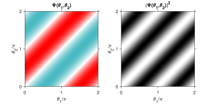
Figure 1: Left: Wavefunction of the singlet state from Eq.(4). Blue is negative, red is positive. Right: Correlated probability distribution of the singlet state from Eq.(5). White is zero, black is maximum.

As can be seen from the previous two equations or from the plots, the wavefunction and correlated probability distribution depend only on the relative angle $\Delta\theta$ between the coordinates at the isolated detectors. This is the core of the Bell inequalities. The original Bell inequality Bell and the CHSH CHSH version are procedures to test for this property. I’ll call the underlying symmetry, that the probability of correlated detection only depends on the relative angle $\Delta\theta$ of the two detections, the Bell correlation. Assuming that the singlet state represents two independent classical objects with individual hidden variables, the specific symmetry of the corresponding classical probability distribution can not reproduce the Bell correlation Bell .

II Quantum Relativity and Elements of Classical Reality

• “We do not describe the world we see, we see the world we can describe.”

  - René Descartes

• “As for my own opinion, I have said more than once, that I hold space to be something merely relative, as time is, that I hold it to be an order of coexistences, as time is an order of successions.”

  - Gottfried Leibniz

If the perspective is taken that only the single relative coordinate between the two detection events exists for quantum events, then constructing a classical distribution that exhibits the Bell correlation is trivial—it would satisfy the Bell correlation by construction. In order to make sense of the Bell situation, one way forward then is to add to quantum mechanics the additional postulate that only the relative coordinates between experimental settings are valid observables when comparing correlated measurements of quantum events. In this way, violations of Bell inequalities arise because the quantum world has fundamentally less degrees-of-freedom for the hidden variables than Bell had assumed. He was averaging over additional non-existent classical configurations in deriving the classical side of the inequality. This is the meaning of the Copenhagen interpretation—if you can not measure it, it effectively does not exist. In this sense, EPR EPR and Bohr Bohr are both correct. There really is nothing beyond the quantum, but quantum mechanics could be considered incomplete in that it was missing a postulate.

The postulate can also be thought of as a quantum relativity principle where only the relative coordinates of experimentally-detected quantum events have a real classical existence. This statement will be called “weak” quantum relativity. A “full” version will be introduced below. Consider doing a Bell experiment in a completely empty universe where nothing exists except the detectors and the singlet state. Only the relative angle between the detection events could exist in this universe since there is nothing else in it to define another angle against. Even if the two detectors are classically connected to the entire universe, there still isn’t a reference to measure anything except a single relative coordinate. Alternatively, think of measuring the position and momentum of a quantum particle. Detecting a quantum event at a single point on a position-sensitive screen gives you information about position, but absolutely no information about momentum. To be a full element of classical reality requires that a particle have both position and momentum simultaneously, but a single detection point clearly does not have a momentum. Therefore, a single quantum event does not carry a full element of classical reality.

What then is a quantum event? A single measured quantum event must be correlated with a second quantum event in order to be a valid element of classical reality. What have been called quantum particles are not full elements of classical reality. Rather, it is actually the correlations between the quantum particles that must be considered as the full elements of reality within the classical description of the world. One pair of correlated quantum events carries one element of correlation, and one element of correlation is only one element of classical reality.

III Uncertainty Principles

For clarity, it is useful to start with sound as an analogy. Sound can be represented as a single value that depends on time, $S(t)$, or as a single value that depends on frequency, $\tilde{S}(f)$, but not both. Gabor showed Gabor how this property leads to an uncertainty principle between $t$ and $f$. He believed that his treatment of acoustics was simply a curious mathematical analogy and did not suggest a serious connection with quanta of the atomic world.

Frequencies and times do not exist independent of each other. We write music as a series of pitches that occur at different times, but this is not really what is happening. Music is defined not by absolute pitch occurring at different times, but more by relative pitches changes that occur at the correct time intervals. This is why any particular song is recognizable as long as all the frequency intervals remain the same. Transposing to a different pitch does not change the song (though it might change the mood of the song as you perceive it). Likewise, any particular song will be recognizable if it is shifted in time (though you might not be in the mood to perceive it at all times).

The analogous situation holds true for position and momentum of quantum point particles. The path of a point object is fully characterized by a single coordinate, say $x(t)$ or $p(t)$, but not both. One can be derived from the other as long as we are only interested in intervals between positions and/or momenta at different points in time. In analogy with the uncertainty principle for sound, this leads to the existence of the Heisenberg uncertainty principle between $x$ and $p$ of a quantum coordinate. Uncertainty relations arise when we attempt a description of reality that is overcomplete. Only relative distances and relative momenta carry meaning when we measure the world.

The Heisenberg uncertainty principle also follows from the recognition that we are only really able measure positions and times of events, that we live in space-time. Consider measuring the momentum of an object. To do so in practice requires measuring some property of that object at two points in space-time, say for example the center-of-mass coordinate at two different times

$$p(t)=M\frac{x_{cm}(t+\Delta t)-x_{cm}(t)}{\Delta t}$$ (6)

where $M$ is the mass of the object. When momentum is measured, it is really relative distances and relative times that are being measured. Position and momentum are not independent of each other.

IV Building the Classical world

• “If you with to make an apple pie from scratch, you must first invent the universe.”

  - Carl Sagan

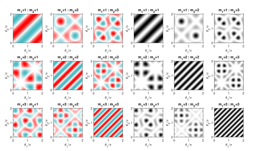
Figure 2: Wavefunctions (blue negative, red positive) and correlated probability distributions (white zero, black maximum) for a variety of negative excited-state singlets.

Can quantum relativity be reconciled with the apparent observation that classical correlations, and not Bell correlations, seem to exist all around us? That is, can the quantum relativity principle help us explain the quantum to classical transition? Let’s invent the classical universe.

Returning to the double-rotor system, allow the fragments to carry more than one unit of angular momentum. Let the system break apart from some unknown initial state into the state

$$\langle\theta_{1},\theta_{2}|\psi\rangle = \cos(m_{2}\theta_{1})\sin(m_{1}\theta_{2})$$ (7)

$$-\sin(m_{1}\theta_{1})\cos(m_{2}\theta_{2})$$

where $m_{1}$ and $m_{2}$ are the total angular momenta of each fragment. These are like excited-state singlets. A physical scenario that creates excited-state singlets using spatial coordinates is presented below when considering EPR-type dissociated diatomic scenarios. The correlated probability distribution for measurements of the two observed angles $\theta_{1}$ and $\theta_{2}$ is

$$|\langle\theta_{1},\theta_{2}|\psi\rangle|^{2} = \big{|}\cos(m_{1}\theta_{1})\sin(m_{2}\theta_{2})$$ (8)

$$-\sin(m_{2}\theta_{1})\cos(m_{1}\theta_{2})\big{|}^{2}.$$

The correlated distribution can not in general be written as a function of just the relative angle $\Delta\theta$ for all combination of $m_{1}$ and $m_{2}$. Consequently, some combinations of $m_{1}$ and $m_{2}$ will not show Bell correlations nor be able to violate a Bell inequality.

To elaborate on this point and the symmetries that appear in the distributions defined by Eq.(8), Fig.(2) shows the double-angle wavefunctions and correlated distributions for a variety of fragment momenta $m_{1}$ and $m_{2}$. Two clear symmetries can be seen. One set has wavefunctions that can be written as a function of the single relative coordinate $\Delta\theta$ with corresponding distributions that display Bell correlations. This set can violated of a Bell inequality. The other set has wavefunctions that can not be written as a function of a single relative coordinate and distributions that do not display Bell correlations. This set can not violate a Bell inequality.

From these two classes of symmetries, two classes of coordinates can be recognized: quantum and classical. Quantum coordinates arise when $m_{1}=m_{2}$ and display Bell correlations. Classical coordinates arise when $m_{1}\neq m_{2}$ and do not have the Bell correlations. The quantum or classical nature of the coordinates being measured depends of the type of initial state prepared, and therefore the design of the experiment controls whether quantum of classical effects can be seen in the measured coordinates.

Note also that the symmetry of the wavefunctions is fermionic-like under exchange of experimental coordinates.

V Positive Singlet States

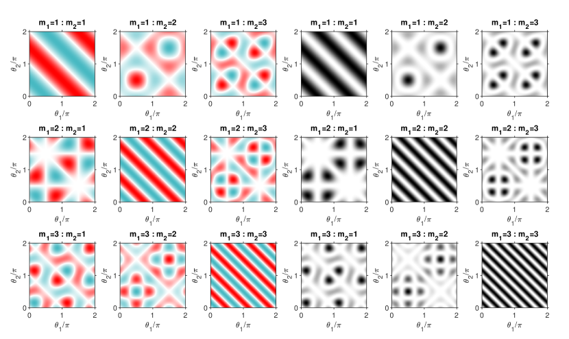
Figure 3: Wavefunctions (blue negative, red positive) and correlated probability distributions (white zero, black maximum) for a variety of positive excited-state singlets.

Instead of negative singlets $|A\rangle|B\rangle-|B\rangle|A\rangle$, consider now positive singlets $|A\rangle|B\rangle+|B\rangle|A\rangle$. For the rotor system, the wavefunctions and correlated distributions of these states are

$$\langle\theta_{1},\theta_{2}|\psi\rangle = \cos(m_{1}\theta_{1})\sin(m_{2}\theta_{2})$$ (9)

$$+\sin(m_{2}\theta_{1})\cos(m_{1}\theta_{2})$$

and

$$|\langle\theta_{1},\theta_{2}|\psi\rangle|^{2} = \big{|}\cos(m_{1}\theta_{1})\sin(m_{2}\theta_{2})$$ (10)

$$+\sin(m_{2}\theta_{1})\cos(m_{1}\theta_{2})\big{|}^{2}.$$

They are plotted in Fig.3. There are again classical-type distributions appearing for $m_{1}\neq m_{2}$ that can not be factorized into a single relative coordinate, but now the quantum-like $m_{1}=m_{2}$ states depend only on the sum of the two experimental coordinates $\theta_{sum}=\theta_{1}+\theta_{2}$ instead of $\Delta\theta$. I’ll call this symmetry the anti-Bell correlation. This symmetry could also violate a Bell inequality that was properly constructed specifically for this state.

Here is where full quantum relativity can be stated: There is only a single classically-real correlation contained in the coordinates of a pair of quantum events. This correlation can appear in either the negative ($\theta_{1}-\theta_{2})$ or positive ($\theta_{1}+\theta_{2})$ correlation of the detector coordinates, but not both. Two quantum events equals one element of correlation, one element of classical reality.

While the negative singlet wavefunctions had fermionic character, the positive singlets have bosonic character—they are symmetric under exchange of coordinates. The bosonic or fermionic character of correlated experimental coordinates depends on the character of the singlet state being measured.

VI The Dissociated Diatomic

Consider now an example closer to the original EPR state EPR , a dissociated homonuclear diatomic. Let $\varphi_{n}(r)$ be the initial eigenstate of the bond length coordinate

$$r=r_{1}-r_{2}$$ (11)

before dissociation, and $\psi(R)$ be the wavefunction of the center-of-mass coordinate

$$R=(r_{1}+r_{2})/2.$$ (12)

The total wavefunction is then

$$\Psi(r,R)=\psi(R)\varphi_{n}(r).$$ (13)

Let the diatomic dissociate into two identical neutral atoms, located at $r_{1}$ and $r_{2}$, that subsequently fly apart. In general, writing out the wavefunction explicitly in terms of $r_{1}$ and $r_{2}$ would yield a non-separable expression for all but a small set of functions $\phi(R)$ and $\varphi_{n}(r)$. However, the state is trivially always separable in $R$ and $r$ simply by construction, so the wavefunction can be written as

$$\Psi(r_{1},r_{2})=\psi(R(r_{1},r_{2}))\varphi_{n}(r(r_{1},r_{2})).$$ (14)

Since it was postulated that the two atoms at $r_{1}$ and $r_{2}$ are identical, which experimentally means that they each can be detected with the same type of detector, there should not be a difference if the two detectors are exchanged. Hence, the wavefunction must be written as

$$\Psi(r_{1},r_{2}) = \psi(R(r_{1},r_{2}))\varphi_{n}(r(r_{1},r_{2}))$$ (15)

$$\pm\psi(R(r_{2},r_{1}))\varphi_{n}(r(r_{2},r_{1})).$$

This is now in the form of an excited-state singlet similar to Eq.(7). Whether the dissociated fragments become a negative or positive singlet depends on the nature of the initial diatomic.

As in Figs.2 and 3 for the double-rotor case, the classical or quantum nature of the atomic fragments following dissociation will depend on the nature of the singlet state Eq.(15). For all but a small set of $\psi(R)$ and $\varphi_{n}(r)$, Eq.(15) will not display Bell correlations and hence $r_{1}$ and $r_{2}$ will behave classically in most cases. It should be possible experimentally to prepare various states of the singlet Eq.(15) by first exciting a beam of diatomics to specific energy eigenstates to control $\varphi(r)$, passing the beam through a double-slit to imprint sturcture onto $\psi(R)$, and then dissociating the diatomics after the slits.

VII Double-Slit Experiments

What is generally being measured in double-slit experiments is the correlated probability distribution between the initial position $\vec{x}_{i}$ at the particle jet and the final position on a detection screen $\vec{x}_{f}$

$$P(\vec{x}_{f},\vec{x}_{i})=\left\langle\vec{x}_{f}\left|\widehat{DS}\right|\vec{x}_{i}\right\rangle.$$ (16)

There are two orthogonal pathways for each possible combination of $\vec{x}_{i}$ and $\vec{x}_{f}$. The pathways are ”through slit 1, miss slit 2” and ”miss slit 1, through slit 2”. The quantum operator for the double-slit process can then be written as

$$\widehat{DS}=|T\rangle|M\rangle\langle T|\langle M|+|M\rangle|T\rangle\langle M|\langle T|$$ (17)

where $|T\rangle$ means the particle went through the slit, and $|M\rangle$ means the particle missed the slit. $\widehat{DS}$ can be further factorized into

$$\widehat{DS}=|\Psi_{DS}\rangle\langle\Psi_{DS}|$$ (18)

where

$$|\Psi_{DS}\rangle=|T\rangle|M\rangle+|M\rangle|T\rangle$$ (19)

is a positive singlet state. This is the origin of the quantum effects seen in the double-slit experiment—it is a measurement of a singlet state created by the slit. Within quantum relativity, all quantum effects comes from an experimental realization of a singlet state.

If the screen is placed directly after the slits, then the measured distribution is

$$P_{near}(\vec{x}_{f},\vec{x}_{i}) = \langle\vec{x}_{f}|\Psi_{DS}\rangle\langle\Psi_{DS}|\vec{x}_{i}\rangle$$ (20)

$$= \left|\delta(x_{s}{\rm-}d/2)+\delta(x_{s}{\rm+}d/2)\right|^{2}$$

where the slits are represented with $\delta$-functions. In practice, finite slits would imprint a narrow but finite double-peak shape upon the wavefunction. When measured with the screen placed far from the slits, the measured distribution can be written as

$$P_{far}(\vec{x}_{f},\vec{x}_{i}) = \langle\vec{x}_{f}|\Psi_{DS}\rangle\langle\Psi_{DS}|\vec{x}_{i}\rangle$$ (21)

$$= \cos^{2}\left(\frac{d}{2}\frac{p_{0}}{\hbar}\sin\theta\right).$$

Both of these measured distributions are characterized only by relative parameters. In Eq.(20), $x_{s}$ is the position along the axis that passes through each slit as measured relative to the center of the slits, and $d$ is the distance between the slits. In Eq.(21), $\theta$ is the angle of the detection position relative to the axis that intersects the center of the slits, and $p_{0}$ is a prior characterization of the average momentum of the beam that relies on many relative measurements. Expressing the measured distribution of quantum detection events in terms of only relative coordinates of the detection events is the weak quantum relativistic perspective. Alternatively, the distribution Eq.(20) can be seen as depending only on the sum ($s{\rm+}d/2$) and difference ($s{\rm-}d/2$) of detection coordinates—this is the full quantum relativistic perspective. One can switch between the weak and full perspectives with a coordinate transformation.

It is important to note that if the whole double-slit experiment is shifted in space, no one would expect the probability distributions to change. The double-slit experiment does not care about the absolute position of the experiment. This is analogous to what is happening in the traditional Bell scenario. In Bell experiments there is an angle invariance that reflects the fact that the measured probability distribution is independent of absolute angle.

When trying to measure which slit the particles passed through, the interference pattern at the far screen is removed. For example, maybe in the case of a double-slit experiment with electrons one could flip the spin as it passes one of the slits but not the other. Then the detections on the screen could be correlated with events where the spin-flipper triggers, which would give information about which slit the electron passed. This experiment is now described by

$$P^{(s)}(\vec{x}_{f},s_{f},\vec{x}_{i},s_{i})=\left\langle\vec{x}_{f},s_{f}\left|\widehat{DS}\right|\vec{x}_{i},s_{i}\right\rangle$$ (22)

where $s_{i}$ and $s_{f}$ are the initial and final spin coordinates of the electron, and the $(s)$ superscript implies this is for the spin-coupled version of the double-slit. The pathways are now ”through slit 1, miss slit 2, no spin flip” and ”miss slit 1, through slit 2, flip spin”. Assuming that the initial spin of the electron beam is uniform, the quantum operator for the spin-coupled double-slit process is

$$\widehat{DS}^{(s)} = |T\rangle|M\rangle|\alpha\rangle\langle T|\langle M|\langle\alpha|$$ (23)

$$+|M\rangle|T\rangle|\beta\rangle\langle M|\langle T|\langle\alpha|$$

where the $|\alpha\rangle$ and $|\beta\rangle$ are the two possible spin states, and the incident electron beam was prepared in the $|\alpha\rangle$ state. Unlike $\widehat{DS}$, $\widehat{DS}^{(s)}$ is not separable into a process built from a singlet state. This results in two possible processes as seen by the detection screen,

$$\widehat{DS}^{(\alpha)}=|T\rangle|M\rangle\langle T|\langle M|$$ (24)

and

$$\widehat{DS}^{(\beta)}=|M\rangle|T\rangle\langle M|\langle T|,$$ (25)

that do not interfere like in the singlet case but instead represent two different classical pathways that occur by chance. From the quantum relativity perspective, since this process does not require a singlet description it should not display any quantum effects.

When it is said that quantum particles of a given species are indistinguishable, what is really indistinguishable are particular dichotomic pathways that exist in the singlet state being prepared by experiments designed to measure those quantum particles. If these pathways are indistinguishable, then the related relative coordinates being measured behave like quantum coordinates. If the pathways are distinguishable through coupling to existing internal observed variables, then the coordinates behave like classical coordinates.

VIII Additional Thoughts and Incomplete Speculations

Relative vs Absolute Reference Frames: There seems to have been a discussion between Newton and Leibniz regarding the nature of space-time. Newton argued for an absolute coordinate system, a world stage on which his physical laws played out. Leibniz argued that only relationships between physical objects exist, that the world is fundamentally relative. While special and general relativity as well as quantum field theory removed the dependence of physical laws from an absolute reference frame for 4D macroscopic space-time, they still lacked a full relativistic view of the relationships between microscopic degrees-of-freedom. They are formulated in mixed reference frames. How are the relative and absolute world views related? Perhaps what appears local and causally-related and in a relative world appears non-local and non-causal from an absolute frame and vice versa.

Gravity and QFT: Within quantum relativity, gravity could be an emergent phenomena, not something fundamental. When we see an object or star with our eyes, we are not measuring the object or star. Rather, we are measuring the massless photons that were coupled to the object or star. Mass is directly related to the degrees-of-freedom that we do not see. This is consistent with $M=E_{i}(\vec{q}_{i})/c^{2}$, where what we call internal energy $E_{i}$ is expressible in terms of relative coordinates $\vec{q}_{i}$ that are fully internal to the object. Massive objects derive their mass from the existence of potentially-observable but currently-unobserved degrees-of-freedom that they carry. Perhaps a photon is effectively massless because it carries no further possible internal structure, although this does seem to leave the origin of polarization as an open question.

Quantum relativity might help remove infinities in quantum field theory and general relativity. Maybe no longer a need for renormalization or black hole core infinities in our descriptions? Do the infinities in QFT and GR arise from assuming infinite deegrees-of-freedom somewhere? A quantum relativistic description can be finite by construction.

Black hole information loss and Hawking radiation could be analogous to burning a page of writing to destroy the measurable classical information with the combustion fumes being analogous to the radiation. The underlying fundamental degrees-of-freedom of the objects that fall into a black hole can not be destroyed (quantum information can not be destroyed), but the observed relations between them (the classically-measurable relationships between the degrees-of-freedom) are lost.

- (1) A. Einstein, B. Podolsky, and N. Rosen, Phys. Rev. 47, 777 (1935).
- (2) N. Bohr, Phys. Rev. 48, 696 (1935).
- (3) J. Bell, Physics 1, 195 (1964).
- (4) J.F. Clauser, M.A. Horne, A. Shimony, and R.A. Holt, Phys. Rev. Lett. 23, 880 (1969).
- (5) D. Gabor, Nature 159, 591 (1947).