The Impact of Star-Formation-Rate Surface Density on the Electron Density and Ionization Parameter of High-Redshift Galaxies

Abstract

We use the large spectroscopic dataset of the MOSFIRE Deep Evolution Field (MOSDEF) survey to investigate some of the key factors responsible for the elevated ionization parameters ($U$) inferred for high-redshift galaxies, focusing in particular on the role of star-formation-rate surface density ($\Sigma_{\rm SFR}$). Using a sample of 317 galaxies with spectroscopic redshifts $z_{\rm spec}\simeq 1.9-3.7$, we construct composite rest-frame optical spectra in bins of $\Sigma_{\rm SFR}$ and infer electron densities, $n_{e}$, using the ratio of the [O II] $\lambda\lambda 3727,3730$ doublet. Our analysis suggests a significant ($\simeq 3\sigma$) correlation between $n_{e}$ and $\Sigma_{\rm SFR}$. We further find significant correlations between $U$ and $\Sigma_{\rm SFR}$ for composite spectra of a subsample of 113 galaxies, and for a smaller sample of 25 individual galaxies with inferences of $U$. The increase in $n_{e}$—and possibly also the volume filling factor of dense clumps in H II regions—with $\Sigma_{\rm SFR}$ appear to be important factors in explaining the relationship between $U$ and $\Sigma_{\rm SFR}$. Further, the increase in $n_{e}$ and SFR with redshift at a fixed stellar mass can account for most of the redshift evolution of $U$. These results suggest that the gas density, which sets $n_{e}$ and the overall level of star-formation activity, may play a more important role than metallicity evolution in explaining the elevated ionization parameters of high-redshift galaxies.

I. INTRODUCTION

Spectroscopic surveys of the rest-frame optical nebular emission lines of redshift $1\lesssim z\lesssim 7$ galaxies have enabled detailed characterization of the physical state of the interstellar medium (ISM) and its evolution from the epoch of peak star formation to the present day. One important observational finding of these surveys is the general increase in the ionization parameter (at a fixed stellar mass) with redshift (e.g., Brinchmann et al. 2008; Nakajima et al. 2013; Steidel et al. 2014; Shirazi et al. 2014; Shapley et al. 2015; Kewley et al. 2015; Bian et al. 2016; Sanders et al. 2016; Kashino et al. 2017; Kojima et al. 2017; Kaasinen et al. 2018; Strom et al. 2018; Topping et al. 2020b; Runco et al. 2021), where the ionization parameter is defined as:

$$U\equiv\frac{n_{\gamma}}{n_{\rm H}},$$ (1)

where $n_{\gamma}$ and $n_{\rm H}$ are the hydrogen-ionizing photon and hydrogen gas densities, respectively. For an ionization-bounded H II region, $U$ can be written as function of the ionizing photon rate ($Q$), electron density ($n_{e}$), and the volume filling factor of the line-emitting gas ($\epsilon$):

$$U\propto[Qn_{e}\epsilon^{2}]^{1/3}$$ (2)

(Charlot & Longhetti, 2001; Brinchmann et al., 2008). The redshift evolution of the ionization parameter at fixed stellar mass is typically attributed to lower gas-phase oxygen (O) abundances, harder ionizing spectra (reflective of lower stellar metallicities and/or younger ages), and/or higher gas (or electron) densities characteristic of high-redshift galaxies.

In particular, several recent investigations have used density-sensitive probes—such as the ratios of the [O II] or [S II] doublet lines—to infer electron densities ($n_{e}$) that are elevated by up to an order of magnitude at $z\sim 1-2$ relative to typical star-forming galaxies in the local universe (e.g., Lehnert et al. 2009; Masters et al. 2014; Steidel et al. 2014; Shimakawa et al. 2015; Bian et al. 2016; Steidel et al. 2016; Sanders et al. 2016; Davies et al. 2021). The apparent evolution of $n_{e}$ may be tied to the higher star-formation rates (SFRs), specific SFRs, and/or SFR surface densities ($\Sigma_{\rm SFR}$) of high-redshift galaxies. For example, Brinchmann et al. (2008), Liu et al. (2008), Masters et al. (2016), and Bian et al. (2016) found that nearby galaxies that are offset in the same direction as high-redshift galaxies from the local star-forming sequence in the $\text{[{O~{}III}]}/\text{H$\beta$}$ versus $\text{[{N~{}II}]}/\text{H$\alpha$}$ BPT plane exhibit higher $\Sigma_{\rm SFR}$ and/or $n_{e}$. Further, Kaasinen et al. (2017) highlighted the similarity in $n_{e}$ of local and high-redshift galaxies when matched in SFR. Shimakawa et al. (2015) used a small sample of 14 H$\alpha$ emitters at $z=2.5$ to directly demonstrate a significant correlation between $n_{e}$ and $\Sigma_{\rm SFR}$, one that has been subsequently confirmed to exist for local analogs of high-redshift Ly$\alpha$ emitters (“Green Pea” galaxies) and local Lyman-break analogs (Jiang et al. 2019; see also Herrera-Camus et al. 2016). Similarly, based on data from the KMOS-3D survey, Davies et al. (2021) suggest that the redshift evolution of $n_{e}$ may be tied to the increasing density of molecular clouds.

Thus, aside from an increase in ionizing photon rates, the higher $\Sigma_{\rm SFR}$ (or molecular gas densities) characteristic of high-redshift galaxies, accompanied by higher $n_{e}$, may be partly responsible for the elevated ionization parameters inferred for $z\sim 2$ galaxies (e.g., Shirazi et al. 2014; Bian et al. 2016; Reddy et al. 2022). Unfortunately, the physical interpretation of correlations between ionization parameter and other global galaxy properties (e.g., $\Sigma_{\rm SFR}$) is complicated by the fact that the ionization parameter is not directly observable. Rather, it is usually inferred using photoionization modeling with simplified (plane-parallel or spherical) geometries that do not faithfully capture the complicated structure of real H II regions (e.g., Pellegrini et al. 2011; see also discussion in Sanders et al. 2016). As a result, the ratio of emission lines from two different ionization stages of the same element is often used as proxy for the ionization parameter. Examining such line ratios can give useful insights into the primary factors that modulate the ionization parameter in high-redshift galaxies.

In this paper, we use the MOSFIRE Deep Evolution Field (MOSDEF) spectroscopic survey data (Kriek et al., 2015) in the CANDELS fields (Grogin et al., 2011; Koekemoer et al., 2011) in addition to predictions of photoionization models to investigate a few of the relevant factors responsible for the elevated ionization parameters inferred for high-redshift galaxies. The MOSDEF survey is particularly well-suited to address this issue since it targets many of the strong rest-frame optical emission lines that probe the ionization parameter, gas-phase oxygen abundance, and electron density. In addition, rest-frame FUV spectroscopy of a subsample of MOSDEF galaxies (MOSDEF-LRIS; Topping et al. 2020b; Reddy et al. 2022) enables direct constraints on the hardness of the ionizing spectra of the same galaxies. Finally, the deep HST imaging that exists in the CANDELS fields enables measurements of $\Sigma_{\rm SFR}$. All these elements together form an ideal dataset with which to study the evolving relationships between stellar metallicities, ages, SFRs, stellar masses, gas-phase abundances, and ionization parameters (Shapley et al., 2015; Sanders et al., 2015, 2016, 2018; Topping et al., 2020b; Runco et al., 2021).

Here, we extend these previous efforts by focusing on how electron densities and ionization parameters correlate with $\Sigma_{\rm SFR}$, and investigating the relative importance of electron or gas density in explaining the variation in ionization parameters inferred for high-redshift galaxies. Section II summarizes the MOSDEF survey and the samples analyzed in this work. Sections III and IV present our findings regarding correlations between electron density and $\Sigma_{\rm SFR}$, and between ionization parameter and $\Sigma_{\rm SFR}$, respectively. The implications of our results for the variation in $U$ among galaxies in our sample, and the redshift evolution of $U$, are discussed in Section V. The conclusions are presented in Section VI. A Chabrier (2003) initial mass function (IMF) is considered throughout the paper. Wavelengths are reported in the vacuum frame. We adopt a cosmology with $H_{0}=70$ km s^-1 Mpc^-1, $\Omega_{\Lambda}=0.7$, and $\Omega_{\rm m}=0.3$.

II. SAMPLE

The galaxies analyzed here were drawn from the MOSDEF survey (Kriek et al., 2015). This survey targeted $\approx 1500$ H-band-selected galaxies and AGNs at redshifts $1.4\lesssim z\lesssim 3.8$ in the CANDELS fields (Grogin et al., 2011; Koekemoer et al., 2011) with moderate resolution ($R\sim 3000-3600$) rest-frame optical spectroscopy using the MOSFIRE spectrometer (McLean et al., 2012) on the Keck telescope. Details of the survey, spectroscopic data reduction, and line flux measurements are provided in Kriek et al. (2015) and Reddy et al. (2015).

The analysis of electron densities (Section III) is based on the subset of MOSDEF galaxies with secure spectroscopic redshifts $z_{\rm spec}\geq 1.9$; no evidence of AGN based on the criteria of Coil et al. (2015), Azadi et al. (2017, 2018), and Leung et al. (2019); spectral coverage and no significant sky line contamination of [O II] $\lambda\lambda 3727,3730$; and reliable half-light radii, $R_{\rm eff}$, and their measurement uncertainties based on the size catalogs of van der Wel et al. (2014). These criteria result in a “density” sample consisting of 317 galaxies which span the full range of SFR and $M_{\ast}$ as the parent MOSDEF sample.

The analysis of the ionization parameter (Section IV) is based on the subset of MOSDEF galaxies with secure spectroscopic redshifts $1.59<z_{\rm spec}<2.56$; no evidence of AGN based on the criteria of Coil et al. (2015), Azadi et al. (2017, 2018), and Leung et al. (2019); spectral coverage and no significant sky line contamination of [O II], [O III], H$\beta$, and H$\alpha$; and reliable half-light radii, $R_{\rm eff}$, and their measurement uncertainties based on the size catalogs of van der Wel et al. (2014). These criteria result in an “ionization parameter” sample consisting of 113 galaxies which span the full range of SFR and $M_{\ast}$ as the parent MOSDEF sample. For reference, the distributions of SFR and $M_{\ast}$ for galaxies in the density and ionization parameter samples relative to those of the parent MOSDEF sample are shown in Figure 1.

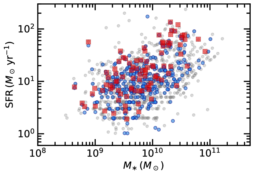
Figure 1.— Distributions of SFR and $M_{\ast}$ for the density and ionization parameter samples (blue and red symbols, respectively) relative to those of the parent MOSDEF sample (grey symbols). The SFRs shown here are mostly based on the H$\alpha$ luminosities corrected for dust based on the Balmer decrement (e.g., Reddy et al. 2015). If such measurements are not available (e.g., H$\alpha$ is not covered and/or H$\alpha$ or H$\beta$ are not significantly detected), then the SFRs are based on modeling the broadband photometry (Section II).

The $R_{\rm eff}$ for galaxies in the two aforementioned samples, along with SFRs calculated from fitting the broadband spectral energy distributions (SEDs) of the galaxies, are used to compute $\Sigma_{\rm SFR}$ as described in Reddy et al. (2022). The SED-inferred SFRs assume the same Binary Population and Spectral Synthesis (BPASS; Eldridge et al. 2017) models discussed in Reddy et al. (2022), where we adopted an SMC attenuation curve for the reddening of the stellar continuum.

Table 1Density Subsamples

Subsample	$N$	$\langle\Sigma_{\rm SFR}\rangle$	$\langle R\rangle$	$\langle n_{e}\rangle$
		$(M_{\odot}\,{\rm yr}^{-1}\,{\rm kpc}^{-2})$		$({\rm cm}^{-3})$
$\Sigma_{\rm SFR}$,Q1	79	$0.107\pm 0.005$	$1.326\pm 0.101$	$88^{+87}_{-70}$
$\Sigma_{\rm SFR}$,Q2	79	$0.260\pm 0.010$	$1.231\pm 0.064$	$170^{+66}_{-57}$
$\Sigma_{\rm SFR}$,Q3	79	$0.453\pm 0.013$	$1.247\pm 0.068$	$155^{+67}_{-58}$
$\Sigma_{\rm SFR}$,Q4	80	$1.991\pm 0.358$	$1.026\pm 0.066$	$425^{+121}_{-98}$

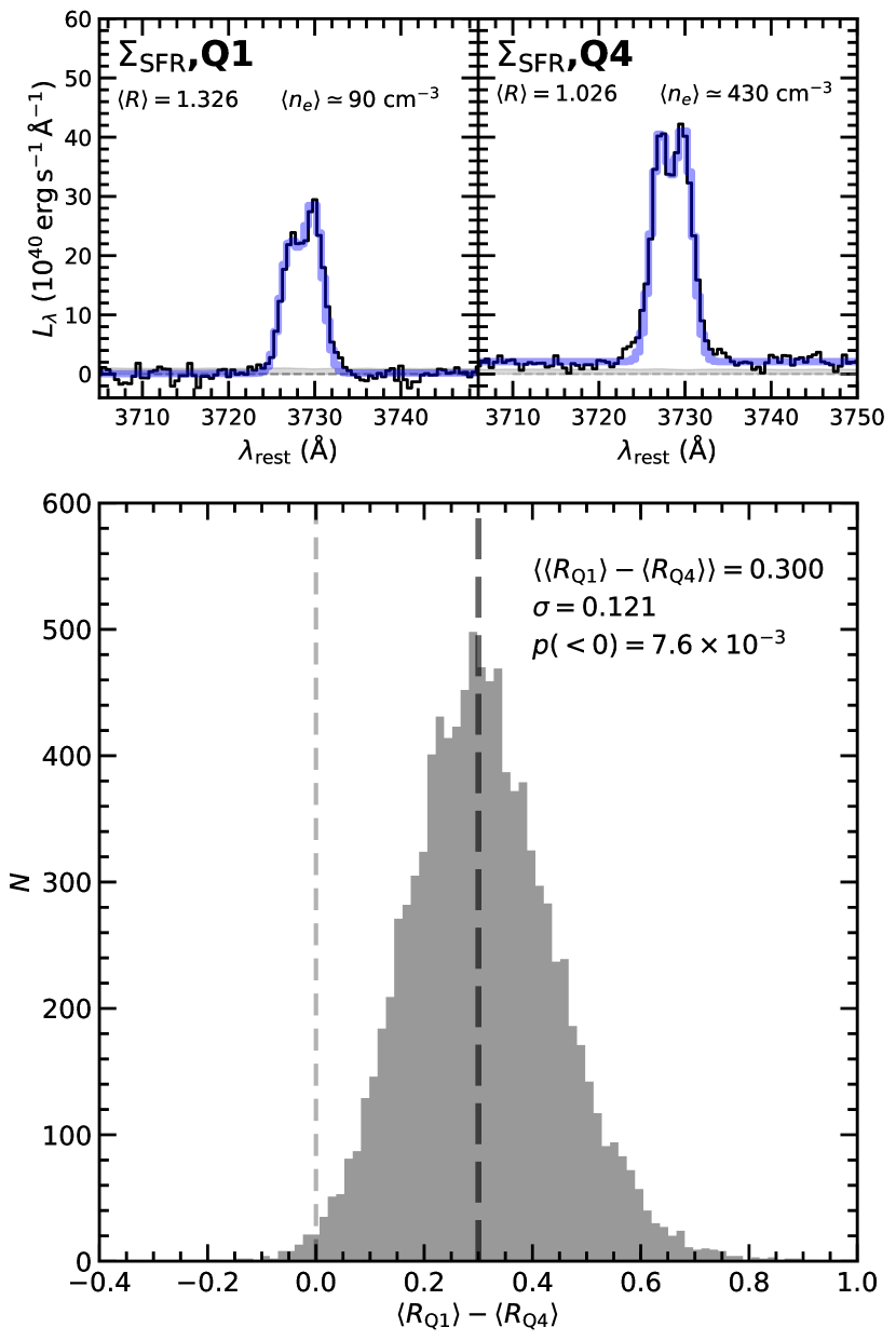
Figure 2.— Top: Composite spectra of the [O II] $\lambda\lambda 3727,3730$ doublet for galaxies in the lowest (left) and highest quartiles (right) of $\Sigma_{\rm SFR}$. The grey shaded regions indicate the composite error spectra. Model fits to the [O II] doublet are indicated in blue, with the average line ratio, $\langle R\rangle=\langle\text{[{O~{}II}]}\,\lambda 3730/\text{[{O~{}II}]}\,\lambda 3727\rangle$, and inferred density, $\langle n_{e}\rangle$, indicated in each panel. Bottom: Distribution of the difference in line ratios measured from 10,000 realizations of the composite spectra in the lowest and highest quartiles of $\Sigma_{\rm SFR}$. The long-dashed line indicates the average difference of $\langle\langle R_{\rm Q1}\rangle-\langle R_{\rm Q4}\rangle\rangle=0.300$. Also indicated are the standard deviation ($\sigma$) and the probability that the average line ratios measured for the two quartiles are equivalent.

III. ELECTRON DENSITY

Electron densities were inferred from the ratio of [O II] $\lambda 3730$ to [O II] $\lambda 3727$ ($R$) as described in Sanders et al. (2016). Robust $n_{e}$ constraints on individual galaxies require extremely high $S/N$ measurements of [O II], higher than what is typically available in the MOSDEF spectra. As a result, we focused on measuring $R$ from composite spectra to obtain the tightest constraints on $n_{e}$. The density sample was divided into four bins of $\Sigma_{\rm SFR}$, each containing roughly an equal number of galaxies. Composite spectra were constructed for galaxies in each of these bins using the methodology described in Reddy et al. (2022). Specifically, individual galaxy spectra were averaged together assuming no weighting in order to avoid biasing the composite to the more luminous galaxies in the sample. The strong rest-frame optical emission lines in the composite spectra for the four bins of $\Sigma_{\rm SFR}$ are shown in Appendix A. $R$ was measured by fitting simultaneously two Gaussian functions to the two lines of the [O II] doublet assuming an intrinsic line width equivalent to that measured for [O III] $\lambda 5008$, and calculating the ratio of the [O II] $\lambda 3730$ line flux to the [O II] $\lambda 3727$ line flux. Uncertainties in $R$ were determined by perturbing individual science spectra by the corresponding error spectra, reconstructing the composite spectra from these individual perturbed spectra many times with replacement, and remeasuring $R$.

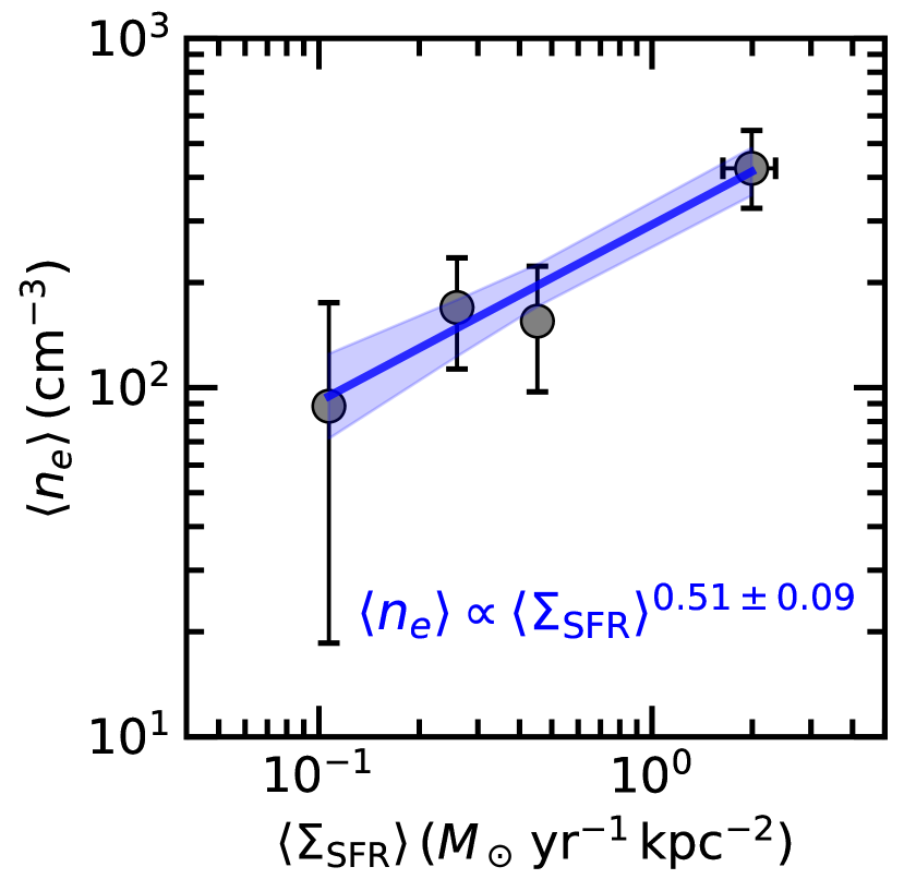
Figure 3.— Average electron density versus average $\Sigma_{\rm SFR}$ for the four quartiles of $\Sigma_{\rm SFR}$. The best-fit power law and $1\sigma$ confidence interval are indicated by the solid blue line and shaded blue region, respectively.

Table 1 lists the number of galaxies in each of the four subsamples, along with the average $\Sigma_{\rm SFR}$, $R$, and the inferred $n_{e}$ for each subsample. The top panels of Figure 2 illustrate the [O II] fits obtained for the bottom and top quartile bins of $\Sigma_{\rm SFR}$. The bottom panel of this figure shows the distribution of the difference in $\langle R\rangle$ for the bottom and top quartile bins of $\Sigma_{\rm SFR}$ obtained from 10,000 realizations of the data. A one-sided $t$ test of this distribution indicates a probability $p\simeq 7.6\times 10^{-3}$ that there is no statistical difference in the [O II] doublet line ratio for the bottom and top quartile bins of $\Sigma_{\rm SFR}$. Electron densities were calculated from the line ratios using the prescription given in Sanders et al. (2016), and are shown in Figure 3.

Our results imply a significant and close to a factor of $5$ increase in $\langle n_{e}\rangle$ for galaxies in the top quartile of $\Sigma_{\rm SFR}$ relative to those in the bottom quartile. A formal fit to $\langle n_{e}\rangle$ versus $\langle\Sigma_{\rm SFR}\rangle$ for the four bins of $\Sigma_{\rm SFR}$ implies

$$\langle n_{e}\rangle\propto\langle\Sigma_{\rm SFR}\rangle^{0.51\pm 0.09}$$ (3)

(Figure 3), consistent with the power-law index of $\approx 0.61$ found by Shimakawa et al. (2015) for a much smaller sample of 14 individual H$\alpha$ emitters at $z=2.5$. The power-law index found here is also consistent (within the $68\%$ confidence intervals) of the index obtained from fitting individual local Lyman break galaxy analogs and Ly$\alpha$ emitters (Jiang et al., 2019). Note that the scaling relation of Equation 3 is based on composite measurements of $n_{e}$. It is possible that outliers in the lowest and highest bins are averaged out in the composites in a way that produces a shallower power-law index than what would have been obtained from fitting individual measurements of $n_{e}$. Consequently, it is possible that the power-law index between $n_{e}$ and $\Sigma_{\rm SFR}$ may be larger than the value found here, strengthening our conclusion of a significant correlation between $n_{e}$ and $\Sigma_{\rm SFR}$. High signal-to-noise measurements of density-sensitive indicators such as [O II] for individual galaxies may be necessary to robustly constrain the power-law index. At any rate, the dependence of ionization parameter on $n_{e}$ (Section IV), the positive correlation between $n_{e}$ and $\Sigma_{\rm SFR}$, and the generally higher $\Sigma_{\rm SFR}$ characteristic of high-redshift galaxies, together may provide an explanation for the elevated ionization parameters inferred at high redshift, a point to which we return to below.

IV. IONIZATION PARAMETER

The ratio of [O III] to [O II], i.e.,

$${\rm O32}=\log\left[\frac{\text{[{O~{}III}]}\,\lambda 4960+\text{[{O~{}III}]}\,\lambda 5008}{\text{[{O~{}II}]}\,\lambda 3727+\text{[{O~{}II}]}\,\lambda 3730}\right]$$ (4)

is commonly used as a proxy for the ionization parameter, $U$ (e.g., Nakajima & Ouchi 2014). Here, we investigate the correlation between $U$ and $\Sigma_{\rm SFR}$, first using O32 as a proxy for the former, and then using estimates of $U$ based on photoionization modeling of individual galaxies.

Figure 4 shows the relationship between O32 and $\Sigma_{\rm SFR}$ for 93 individual galaxies in the “ionization parameter” sample (Section II) with significant (i.e., $S/N\geq 3$) detections of [O II], [O III], H$\beta$, and H$\alpha$. Both [O II] and [O III] were corrected for dust attenuation by applying a reddening correction derived from the Balmer decrement ($\text{H$\alpha$}/\text{H$\beta$}$) and assuming the Cardelli et al. (1989) extinction curve (e.g., Reddy et al. 2020; Rezaee et al. 2021). The Balmer decrements for individual galaxies vary from the theoretical value in a dust-free case, $\text{H$\alpha$}/\text{H$\beta$}\simeq 2.8$, up to $\text{H$\alpha$}/\text{H$\beta$}\simeq 8$ for the dustiest objects in our sample. Also shown in this figure are the average O32 values derived from composite spectra of galaxies in the “ionization parameter” sample in the same four $\Sigma_{\rm SFR}$ bins used to compute $n_{e}$. These average O32 values imply that the relationship between O32 and $\Sigma_{\rm SFR}$ for galaxies with significant detections of the four aforementioned emission lines is not substantially biased relative to that obtained for all 113 galaxies of the “ionization parameter” sample.

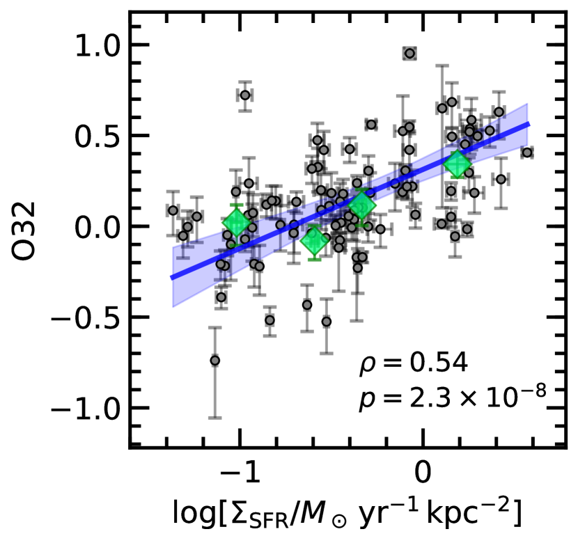
Figure 4.— O32 versus $\log[\Sigma_{\rm SFR}/M_{\odot}\,{\rm yr}^{-1}\,{\rm kpc}^{-2}]$ for 93 galaxies in the “ionization parameter” sample with $S/N\geq 3$ detections of [O II], [O III], H$\beta$, and H$\alpha$ (grey points). A Spearman test on the individual measurements for the 93 galaxies indicates a correlation coefficient of $\rho=0.54$, with a probability $p=2.3\times 10^{-8}$ that there is a null correlation between O32 and $\Sigma_{\rm SFR}$. A linear fit to the data and the $1\sigma$ confidence interval are indicated by the blue line and shaded region, respectively: ${\rm O32}=(0.415\pm 0.064)\log[\Sigma_{\rm SFR}/M_{\odot}\,{\rm yr}^{-1}\,{\rm kpc}^{-2}]+0.307\pm 0.030$. The average O32 values derived from composite spectra of galaxies in three bins of $\Sigma_{\rm SFR}$ are shown by the large green diamonds.

A Spearman test on the individual measurements indicates a significant correlation between O32 and $\Sigma_{\rm SFR}$ for the subsample of 93 galaxies, with a probability $p=2.3\times 10^{-8}$ of a null correlation between the two. At face value, these results imply a highly significant correlation between $U$ and $\Sigma_{\rm SFR}$. However, it is important to assess the degree to which the translation between O32 and $U$ may be affected by other parameters. In particular, a number of studies have investigated the effect of ionizing spectral hardness, gas-phase abundance, and $n_{e}$ on the O32 ratio (e.g., Sanders et al. 2016; Strom et al. 2018). Here, we discuss some of these dependencies in the context of updated stellar population synthesis models that include the effects of stellar binarity (i.e., the binary BPASS models). These models have generally been found to simultaneously reproduce the rest-frame far-UV photospheric features of high-redshift galaxies and their rest-frame optical nebular emission line ratios (e.g., Steidel et al. 2016; Topping et al. 2020b, a; Reddy et al. 2022).

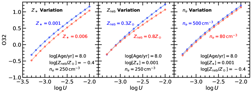
Figure 5.— Predicted relationship between O32 and $\log U$ from photoionization modeling assuming a constant star formation BPASS stellar population model with the indicated stellar metallicity and age, and the indicated nebular oxygen abundance ($Z_{\rm neb}$) and $n_{e}$ (see text).

Figure 5 shows the predicted O32 as a function of $\log U$ for BPASS v2.2.1 constant star formation models with binary stellar evolution and an upper-mass cutoff of the IMF of $100$ $M_{\odot}$ (i.e., the “100bin” models), with the input stellar population and CLOUDY (Ferland et al., 2017) parameters indicated in each panel. For instance, the left panel shows the relationship between O32 and $\log U$ for models with a $\log[{\rm Age/yr}]=8.0$ stellar population, an oxygen abundance of $\log[Z_{\rm neb}/Z_{\odot}]=-0.4$, $n_{e}=250$ cm^-3—all values which are typical of MOSDEF galaxies (e.g., Sanders et al. 2016; Topping et al. 2020b; Reddy et al. 2022)—and two stellar metallicities ($Z_{\ast}=0.001$ and $0.006$, expressed in terms of the mass fraction of metals) that bracket the range inferred from modeling the rest-frame FUV spectra of individual MOSDEF galaxies (Topping et al., 2020a). At a fixed O32, $\log U$ varies by $\simeq 0.15$ dex for the aforementioned range of $Z_{\ast}$. Similarly, the middle panel shows the relationships between O32 and $\log U$ for two values of $Z_{\rm neb}$ that bracket the range where the bulk of MOSDEF galaxies lie (e.g., Topping et al. 2020a) and where the stellar population age, $Z_{\ast}$, and $n_{e}$ are fixed to values typical of MOSDEF galaxies. Finally, the right panel indicates the relationships between O32 and $\log U$ for two values of $n_{e}$ that bracket the range inferred for the MOSDEF sample (Sanders et al. 2016; see also Section III) and where all other parameters are fixed to the typical values. The model predictions summarized in Figure 5 indicate that the translation between O32 and $\log U$ is relatively insensitive to $Z_{\ast}$, $Z_{\rm neb}$, and $n_{e}$ over the ranges of these parameters that are represented in the MOSDEF sample, changing at most by $\simeq 0.15$ dex for a factor of 6 increase in $Z_{\ast}=0.001$ to $0.006$. Thus, the $\simeq 0.8$ dex increase in O32 over the range of $\Sigma_{\rm SFR}$ shown in Figure 4 likely reflects an increase in $U$ with $\Sigma_{\rm SFR}$.

This conclusion is further corroborated by direct modeling of a subset of MOSDEF galaxies with deep rest-frame FUV spectra (i.e., the MOSDEF-LRIS sample; Topping et al. 2020b; Reddy et al. 2022). Reddy et al. (2022) self-consistently modeled the rest-frame FUV spectra and rest-frame optical emission line ratios of galaxies in the MOSDEF-LRIS sample for galaxies in each of three equal-number bins of $\Sigma_{\rm SFR}$. Galaxies in the lower, middle, and upper third of the $\Sigma_{\rm SFR}$ distribution have $\langle{\rm O32}\rangle=-0.03\pm 0.14$, $0.03\pm 0.09$, and $0.33\pm 0.07$, respectively. The modeling of the composite rest-frame FUV spectra of galaxies in these three bins of $\Sigma_{\rm SFR}$ indicates $\langle Z_{\ast}\rangle=0.0013\pm 0.0005$, $0.0021\pm 0.0008$, and $0.0017\pm 0.0004$, respectively (see Table 3 of Reddy et al. 2022). Based on the left panel of Figure 5, this variation in $\langle Z_{\ast}\rangle$ results in a negligible shift in the relationship between O32 and $\log U$. Similarly, $\langle Z_{\rm neb}/Z_{\odot}\rangle=0.28\pm 0.13$, $0.40\pm 0.03$, and $0.43\pm 0.08$, respectively, for the three aforementioned bins of $\Sigma_{\rm SFR}$ (Table 3 of Reddy et al. 2022). Based on the middle panel of Figure 5, this variation in $\langle Z_{\rm neb}\rangle$ also implies a negligible shift in the relationship between O32 and $\log U$. Finally, as per the discussion in Section III, though there is a significant correlation between $n_{e}$ and $\Sigma_{\rm SFR}$, the range of inferred $n_{e}$ implies a negligible shift in the translation between O32 and $\log U$. In summary, the variations in $\langle Z_{\ast}\rangle$, $\langle Z_{\rm neb}\rangle$, and $\langle n_{e}\rangle$ for composites constructed in bins of $\Sigma_{\rm SFR}$ are unlikely to be solely responsible for driving the observed increase in O32 with $\Sigma_{\rm SFR}$ (Figure 4). Rather, this relationship is likely driven by changes in $U$. To that point, Reddy et al. (2022) calculated $\langle\log U\rangle=-3.06\pm 0.07$, $-3.10\pm 0.06$, and $-2.70\pm 0.07$, respectively, for the three bins of $\Sigma_{\rm SFR}$ (Figure 6), implying a significantly higher $\langle\log U\rangle$ for galaxies in the upper third of the $\Sigma_{\rm SFR}$ distribution.

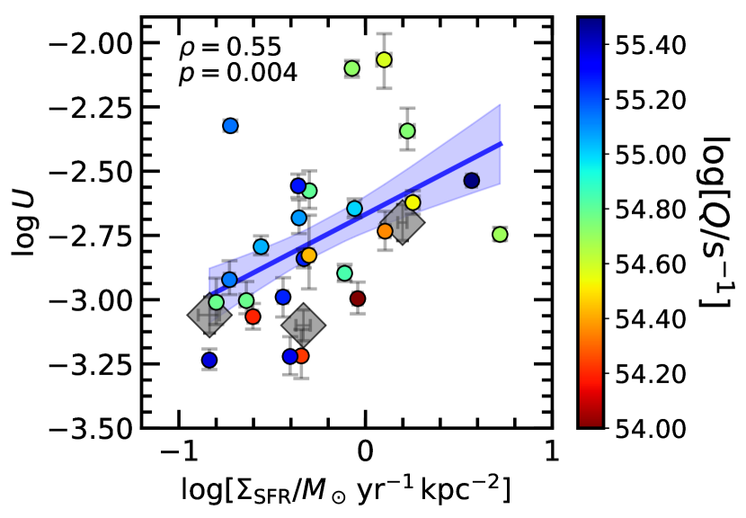
Figure 6.— Relationship between $\log U$ and $\log[\Sigma_{\rm SFR}/M_{\odot}\,{\rm yr}^{-1}\,{\rm kpc}^{-2}]$ for 25 individual galaxies in the MOSDEF-LRIS sample (Topping et al., 2020a) with robust size, and hence $\Sigma_{\rm SFR}$, measurements (circles), and detections of H$\alpha$, color coded by $\log[Q/{\rm s}^{-1}]$ (see Section V.1.1) . The Spearman correlation coefficient and $p$-value are indicated. The solid blue line and shaded region indicate a linear fit to the data and the $1\sigma$ confidence interval, respectively, with the following relation: $\log U=(0.379\pm 0.030)\log\left[\frac{\Sigma_{\rm SFR}}{M_{\odot}\,{\rm yr}^{-1}\,{\rm kpc}^{-2}}\right]-2.668\pm 0.068$. . Average values obtained from fitting composite spectra in three equal-number bins of $\Sigma_{\rm SFR}$ (from Reddy et al. 2022) are shown by the large grey diamonds.

Finally, the relationship between $\log U$ and $\Sigma_{\rm SFR}$ for a subset of 25 individual MOSDEF-LRIS galaxies from Topping et al. (2020a) with robust size measurements and $\text{$L$(H$\alpha$)}/\sigma_{\text{$L$(H$\alpha$)}}\geq 3$, where $L$(H$\alpha$) is the dust-corrected H$\alpha$ luminosity, is shown in Figure 6. A Spearman correlation test indicates a probability of $p=0.004$ that the two variables are uncorrelated, suggesting that the correlation is significant at the $\approx 3\sigma$ level. The figure also shows a linear fit to the data for the individual galaxies.

In summary, the significant correlation between O32 and $\Sigma_{\rm SFR}$ (Figure 4); the insensitivity of the translation between O32 and $U$ to $Z_{\ast}$, $Z_{\rm neb}$, and $n_{e}$ over the range of these parameters represented in the MOSDEF sample (Figure 5); and the differences in average and individually-inferred $U$ for galaxies with low and high $\Sigma_{\rm SFR}$ (Figure 6) altogether suggest a genuine correlation between $U$ and $\Sigma_{\rm SFR}$ (see also Bian et al. 2016; Runco et al. 2021; Reddy et al. 2022).

V. DISCUSSION

In this section, we examine the results on $n_{e}$ and $U$ in the context of the factors that $U$ depends on, including the ionizing photon rate (Section V.1.1), $n_{e}$ (Section V.1.2), the volume filling factor of dense clumps in H II regions (Section V.1.3), and the escape fraction of ionizing photons (Section V.1.4). The implications of our results for the redshift evolution of $U$ are discussed in Section V.2.

V.1. Key Factors that Modulate the Ionization Parameter of High-Redshift Galaxies

Several previous efforts have focused on understanding the factors responsible for the elevated ionization parameters inferred for high-redshift galaxies (e.g., Brinchmann et al. 2008; Bian et al. 2016). Here, we extend upon these previous works by concentrating on the factors responsible for the correlation between $U$ and $\Sigma_{\rm SFR}$ among high-redshift galaxies, taking advantage of the most up-to-date inferences of $n_{e}$, ionizing photon rates ($Q$), volume filling factors ($\epsilon$), and the escape fraction of ionizing photons ($f_{\rm esc}$) for the same galaxies. Equation 2 summarizes the dependencies between $U$ and $Q$, $n_{e}$, and $\epsilon$. Below, we discuss each of these factors, along with $f_{\rm esc}$, in turn.

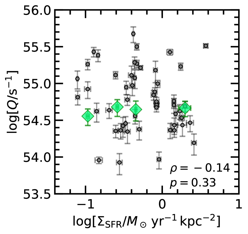
Figure 7.— Relationship between $\log[Q/{\rm s}^{-1}]$ and $\log[\Sigma_{\rm SFR}/M_{\odot}\,{\rm yr}^{-1}\,{\rm kpc}^{-2}]$ for the 51 galaxies in the “ionization parameter” sample with $Q/\sigma_{Q}\geq 3$ (grey points). The Spearman correlation coefficient and $p$-value are indicated. Average values obtained from fitting composite spectra of galaxies in the “ionization parameter” sample in the same four bins of $\Sigma_{\rm SFR}$ used to compute $n_{e}$ are shown by the large green diamonds.

V.1.1 Ionizing Photon Rates ($Q$)

Figure 7 shows the variation in $Q$ with $\Sigma_{\rm SFR}$ for the 51 galaxies in the “ionization parameter” sample with $Q/\sigma_{Q}\geq 3$, where $\sigma_{Q}$ is the uncertainty in $Q$. The Leitherer & Heckman (1995) relation was used to convert dust-corrected $L$(H$\alpha$) to $Q$. Also shown are the average values obtained from composite spectra of the 113 galaxies in the “ionization parameter” sample in the same four bins of $\Sigma_{\rm SFR}$ used to compute $n_{e}$. A Spearman correlation test on the individual measurements of $Q$ and $\Sigma_{\rm SFR}$ imply that the two are not significantly correlated, a result confirmed by the invariance of $\langle Q\rangle$ for the four $\Sigma_{\rm SFR}$ bins.

The ionizing photon rate depends on the SFR and the ionizing photon production efficiency, $\xi_{\rm ion}$ (Robertson et al., 2013; Bouwens et al., 2016; Shivaei et al., 2018; Theios et al., 2019; Reddy et al., 2022): $Q\propto\xi_{\rm ion}\times{\rm SFR}$. The ionizing photon production efficiency depends on the specific details of the massive stars, including their stellar metallicities, ages, whether they evolve as single stars or in binaries, and the IMF. Reddy et al. (2022) showed that $\xi_{\rm ion}$ does not vary significantly with $\Sigma_{\rm SFR}$ for galaxies in the MOSDEF-LRIS sample. This result, combined with the lack of a strong correlation between $L$(H$\alpha$) and $\Sigma_{\rm SFR}$ (note that the latter is based on SED-inferred SFRs; Section II), results in an average $Q$ that is invariant over the dynamic range of $\Sigma_{\rm SFR}$ probed by our sample. Thus, the increase in $U$ with $\Sigma_{\rm SFR}$ cannot be explained by changes in $Q$ alone.

V.1.2 Electron Densities ($n_{e}$)

As noted in Section III and shown in Figure 3, we find a significant correlation between $\langle n_{e}\rangle$ and $\langle\Sigma_{\rm SFR}\rangle$: galaxies with $\langle\Sigma_{\rm SFR}\rangle\simeq 2$ $M_{\odot}$ yr^-1 kpc^-2 have $\langle n_{e}\rangle\simeq 400$ cm^-3, a factor of $\approx 5$ larger than that of galaxies with $\langle\Sigma_{\rm SFR}\rangle\simeq 0.1$ $M_{\odot}$ yr^-1 kpc^-2. For fixed $Q$ and $\epsilon$, this increase in $n_{e}$ corresponds to an $\approx 0.23$ dex increase in $\log U$ based on Equation 2, and accounts for roughly half of the observed $0.4-0.5$ dex increase in $\log U$ over the aforementioned range of $\Sigma_{\rm SFR}$ (Figure 6). Thus, the dependence of $n_{e}$ on $\Sigma_{\rm SFR}$ is an important contributing factor to the dependence of $\log U$ on $\Sigma_{\rm SFR}$.

Note that $n_{e}$ and $\Sigma_{\rm SFR}$ are sensitive to gas on different physical scales. Specifically, $\Sigma_{\rm SFR}$ in the present analysis probes star formation on galactic-wide (kpc) scales, while $n_{e}$ is sensitive to dense structures within pc-scale H II regions. A simple explanation for why the two may correlate is that the Kennicutt-Schmidt relation (Kennicutt, 1998) connects $\Sigma_{\rm SFR}$ to the molecular gas density, and the latter, along with the external ambient density and/or interstellar pressure, determines $n_{e}$ of H II regions (Shirazi et al. 2014; Shimakawa et al. 2015; Kashino & Inoue 2019; Jiang et al. 2019; see further discussion in Davies et al. 2021). Higher spatial resolution measurements of molecular gas and electron densities afforded by nearby galaxies and AO-assisted observations of unlensed and/or lensed galaxies at high redshift should further elucidate the connection between $\Sigma_{\rm SFR}$ and $n_{e}$.

V.1.3 Volume Filling Factors ($\epsilon$)

The variable $\epsilon$ represents the volume filling factor of line-emitting structures within the otherwise diffuse ionized gas in H II regions, and can be approximated by

$$\epsilon\approx[n_{e,{\rm rms}}/n_{e}]^{2},$$ (5)

where $n_{e}$ is the average density of gas giving rise to the [O II] emission and $n_{e,{\rm rms}}$ is the rms electron density in H II regions (Osterbrock & Flather, 1959; Kennicutt, 1984). The latter depends on the volume of H II regions which cannot be directly constrained as individual H II regions are unresolved by our observations. If we assume that H II regions fill the entire star-forming volume, then a lower limit on $n_{e,{\rm rms}}$ can be calculated from the dust-corrected H$\alpha$ luminosity and the (e.g., spherical) volume of ionized gas within a half-light radius, $V_{\text{{H~{}II}}}(<R_{\rm eff})$:

$$n_{e,{\rm rms}}=\left[\frac{\text{$L$(H$\alpha$)}}{2\gamma_{\text{H$\alpha$}}V_{\text{{H~{}II}}}(<R_{\rm eff})}\right]^{1/2},$$ (6)

where $\gamma_{\text{H$\alpha$}}$ is the volume emissivity of H$\alpha$ (e.g., Rozas et al. 1996; Davies et al. 2021). For Case B recombination and $T_{e}=10^{4}$ K, $\gamma_{\text{H$\alpha$}}=3.56\times 10^{-25}$ erg cm³ s^-1. The factor of $2$ in the denominator of Equation 6 accounts for the fact that the volume is calculated based on the half-light radius.

Equations 5 and 6 were used to compute lower limits on $\langle n_{e,{\rm rms}}\rangle$ and $\langle\epsilon\rangle$ from the average H$\alpha$ luminosities and sizes of galaxies in the “ionization parameter” sample in the same four $\Sigma_{\rm SFR}$ bins used to compute $n_{e}$ (Section III). These lower limits span the range $\langle n_{e,{\rm rms}}\rangle\simeq 1$ to $6$ cm^-3 and $\langle\epsilon\rangle\simeq 10^{-4}-10^{-3}$. These values are broadly consistent with the average $n_{e,{\rm rms}}$ and $\epsilon$ found for star-forming galaxies at similar redshifts from the KMOS^3D survey (Davies et al., 2021). Evidently the gas that dominates the line emission likely constitutes a small fraction of the total ionized volume in high-redshift galaxies (see also Kennicutt 1984; Rozas et al. 1996; Elmegreen & Hunter 2000; Copetti et al. 2000; Hunt & Hirashita 2009; Davies et al. 2021). At any rate, given that the $n_{e,{\rm rms}}$ and $\epsilon$ calculated above represent lower limits, we cannot rule out the possibility that there may be a correlation between $\epsilon$ and $\Sigma_{\rm SFR}$ (see Section V.1.5 for further discussion).

V.1.4 Ionizing Escape Fractions ($f_{\rm esc}$)

Line diagnostics that are typically used to infer $U$, such as O32, will overestimate $U$ if there is a non-zero escape fraction of ionizing photons, $f_{\rm esc}$ (Giammanco et al., 2005; Brinchmann et al., 2008; Nakajima et al., 2013). A simple example is the case of a density-bounded nebula where the region of low-ionization emission (e.g., [O II]) is truncated, leading to higher O32 and higher apparent $U$. We can evaluate the magnitude of this effect using recent determinations of $f_{\rm esc}$ at high redshift.

In particular, Reddy et al. (2022) inferred typical average escape fractions of $\langle f_{\rm esc}\rangle\lesssim 10\%$ based on the average depths of Lyman series absorption lines in the composite spectra of galaxies in the MOSDEF-LRIS sample (see also Reddy et al. 2016), with no significant difference in the inferred $\langle f_{\rm esc}\rangle$ for galaxies in the lower- and upper-third of the distribution of $\Sigma_{\rm SFR}$ (e.g., Figure 18 in Reddy et al. 2022). The typical $\langle f_{\rm esc}\rangle$ found in that study is similar to the sample-averaged values of $\langle f_{\rm esc}\rangle\simeq 6-9\%$ derived by Steidel et al. (2018) and Pahl et al. (2021) for a sample of typical star-forming galaxies at $z\sim 3$. Based on the modeling of Giammanco et al. (2005), this low value of $f_{\rm esc}$ results in an apparent $\log U$ that is $\lesssim 0.2$ dex higher than the value when $f_{\rm esc}=0$. This small change in inferred $\log U$, combined with the lack of a significant correlation between $\langle f_{\rm esc}\rangle$ and $\langle\Sigma_{\rm SFR}\rangle$ for galaxies in the MOSDEF-LRIS sample, suggests that the trend between $\log U$ and $\Sigma_{\rm SFR}$ is unlikely to be related to variations in $f_{\rm esc}$.

V.1.5 Summary

The results of the previous sections can be summarized as follows. We find significant correlations between $n_{e}$ and $\Sigma_{\rm SFR}$ (Section III) and between $U$ and $\Sigma_{\rm SFR}$ (Section IV) for typical star-forming galaxies at $z\sim 2$. Thus, $n_{e}$ appears to be an important factor in explaining the correlation between $U$ and $\Sigma_{\rm SFR}$ (Section V.1.2). Of the factors that $U$ depends on, $\epsilon$ is perhaps the most uncertain since it requires knowledge of the volumes of spatially-unresolved H II regions, and we cannot rule out the possibility that $\epsilon$ may also play a role in shaping the correlation between $U$ and $\Sigma_{\rm SFR}$ (Section V.1.3). Indeed, it is not unreasonable to expect that the volume filling factor of H II regions increases with $\Sigma_{\rm SFR}$, in which case $\epsilon$ may play a significant role in driving the relationship between $U$ and $\Sigma_{\rm SFR}$. On the other hand, there is no significant correlation between $Q$ and $\Sigma_{\rm SFR}$ for galaxies in our sample (Section V.1.1), suggesting that changes in the ionizing photon rate are unlikely to contribute to the observed relationship between $U$ and $\Sigma_{\rm SFR}$. Similarly, $f_{\rm esc}$ inferred for galaxies in the sample are too low to account for the significant correlation between $U$ and $\Sigma_{\rm SFR}$ (Section V.1.4).

While $n_{e}$ appears to be an important factor in driving the relationship between $U$ and $\Sigma_{\rm SFR}$ at $z\sim 2$, it is clear that parameters other than $n_{e}$ may be important for explaining the scatter in this relationship. For instance, Figure 6 shows that the five galaxies with the lowest measured $Q$ in the Topping et al. (2020a) sample generally lie below the mean relation between $U$ and $\Sigma_{\rm SFR}$. Thus, variations in $Q$ may be partly responsible for the scatter in the relationship between $U$ and $\Sigma_{\rm SFR}$. Figure 6 also shows that there are some galaxies with similar $\Sigma_{\rm SFR}$ and $Q$, but which have significantly different $U$. This result suggests that variations in $\epsilon$ may also be important for explaining some of the scatter in the relationship between $U$ and $\Sigma_{\rm SFR}$.

V.2. Redshift Evolution of $U$

So far we have focused on the factors that drive the relationship between $U$ and $\Sigma_{\rm SFR}$ for $z\sim 2$ galaxies. We can further explore the extent to which the relationship between $U$ and $\Sigma_{\rm SFR}$ (or $n_{e}$) contributes to the redshift evolution of $U$, as noted by a number of recent studies (Section I). For example, Sanders et al. (2016) noted that typical star-forming galaxies at $z\sim 2$ from the MOSDEF survey have O32 that are on average $\simeq 0.6$ dex higher than local galaxies at a fixed stellar mass. This offset in O32 suggests that $z\sim 2$ galaxies have on average a higher ionization parameter relative to local galaxies at a fixed stellar mass.

In particular, the average O32 of $\sim 10^{10}$ $M_{\odot}$ galaxies at $z\sim 2$ is $\langle{\rm O32}\rangle\simeq 0.1$ (Sanders et al., 2016). Based on the model predictions shown in Figure 5, this average O32 corresponds to $\log U\simeq-3.0$ (see also Topping et al. 2020b; Runco et al. 2021; Reddy et al. 2022). Local star-forming galaxies of the same stellar mass from the SDSS sample have $\langle{\rm O32}\rangle\simeq-0.6$, corresponding to $\log U\simeq-3.6$ (Shirazi et al., 2014; Nakajima & Ouchi, 2014). Thus, at fixed stellar mass of $\sim 10^{10}$ $M_{\odot}$, galaxies at $z\sim 2$ have $\langle\log U\rangle$ that is $\approx 0.6$ dex higher than that of local galaxies. Below, we discuss some of the factors that may be responsible for the redshift evolution of $U$.

V.2.1 The Role of Electron Density and SFR

Sanders et al. (2016) found an order of magnitude increase in $\langle n_{e}\rangle$ for galaxies with stellar masses of $\sim 10^{10}$ $M_{\odot}$ from $z\sim 0$ to $z\sim 2$. In the simple spherical geometry of an ionization-bounded nebula where $U\propto n_{e}^{1/3}$ (Equation 2), such an increase in $n_{e}$ translates to an $\approx 0.3$ dex increase in $\log U$ for a fixed $Q$ and $\epsilon$. Thus, at face value, the redshift evolution of $n_{e}$ could account for a significant fraction of the $\simeq 0.6$ dex increase in $\log U$ for $z\sim 2$ galaxies relative to local galaxies at fixed stellar mass (Brinchmann et al., 2008; Shirazi et al., 2014; Bian et al., 2016).

In addition, there is an $\approx 1$ dex increase in SFR (and hence $Q$, assuming a constant $\xi_{\rm ion}$) between $z\sim 0$ and $z\sim 2$ at a fixed stellar mass of $10^{10}$ $M_{\odot}$ (e.g., Speagle et al. 2014). This redshift evolution of SFR (and $Q$) implies an $\approx 0.3$ dex increase in $\log U$ assuming the scaling relation specified in Equation 2 (see also Nakajima & Ouchi 2014; Kaasinen et al. 2018). Finally, Davies et al. (2021) present evidence that the volume filling factor, $\epsilon$, does not evolve significantly over the redshift range $0\lesssim z\lesssim 2.6$. Hence, the $0.3$ dex increase in $\log U$ due to $n_{e}$ evolution, and the $0.3$ dex increase in $\log U$ due to SFR evolution, together could account for much of the $0.6$ dex increase in $\log U$ from $z\sim 0$ to $z\sim 2$. In the next section, we evaluate this conclusion in the context of previous studies that have underscored the role of metallicity in the redshift evolution of $U$.

V.2.2 The Role of Stellar Metallicity

Several studies have attributed the redshift evolution of $U$ at a fixed stellar mass to changes in metallicity. Specifically, there is a well-established anti-correlation between $U$ and $Z_{\rm neb}$ for local star-forming galaxies (e.g., Dopita & Evans 1986; Dopita et al. 2006; Pérez-Montero 2014) which is usually explained in terms of lower-metallicity massive stars having harder ionizing spectra and more intense radiation fields (Dopita et al., 2006; Leitherer et al., 2014). In this case, $\xi_{\rm ion}$, and hence $Q$ at a fixed SFR, will be larger for lower-metallicity stellar populations. The redshift-invariance of the relationship between $U$ and $Z_{\rm neb}$ (Topping et al., 2020a; Sanders et al., 2020) then implies that the decrease in $Z_{\rm neb}$ with redshift at a fixed stellar mass (i.e., the redshift evolution of the mass-metallicity relation) is accompanied by an increase in $U$ with redshift at a fixed stellar mass (e.g., Sanders et al. 2016). In the following discussion, we examine the extent to which metallicity affects the redshift evolution of $U$.

The ionizing spectra of massive stars are more directly connected to stellar metallicity (or Fe abundance) than O abundance ($Z_{\rm neb}$), since the former dominates the opacity of stellar atmospheres and regulates the launching of stellar winds and the absorption of ionizing photons by those winds (e.g., Dopita et al. 2006). As such, we frame our discussion in terms of $Z_{\ast}$ rather than $Z_{\rm neb}$. Figure 8 shows how $Q$ is predicted to vary with $Z_{\ast}$ for the BPASS 100bin stellar population synthesis models with an age of $10^{8}$ yr and a constant star-formation rate of $1$ $M_{\odot}$ yr^-1. Also indicated are $\langle Z_{\ast}\rangle$ inferred for $z\sim 0$ and $z\sim 2.2$ galaxies with $M_{\ast}\sim 10^{10}$ $M_{\odot}$ based on the relationships between stellar metallicity and stellar mass at those redshifts (Kashino et al., 2022). Based on the model predictions, the difference in $\langle Z_{\ast}\rangle$ inferred at these two redshifts results in $\Delta\log[Q/{\rm s}^{-1}]\simeq 0.23$ dex. If all other parameters affecting $Q$ are held fixed (i.e., the details of the stellar population model including the star-formation history, age, inclusion of binaries, IMF, and SFR), and if $n_{e}$ and $\epsilon$ are held fixed, then the difference in $Z_{\ast}$ between $z\sim 0$ and $z\sim 2.2$ galaxies implies $\Delta\log U\simeq 0.08$ dex assuming $U\propto Q^{1/3}$ (Equation 2).

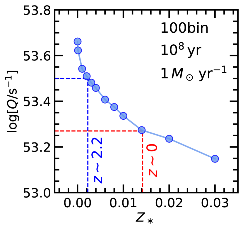
Figure 8.— $Q$ as function of $Z_{\ast}$ for the BPASS 100bin models with an age of $10^{8}$ yr and a constant star-formation rate of $1$ $M_{\odot}$ yr^-1. Also indicated are the $\langle Z_{\ast}\rangle$ inferred for $z\sim 0$ and $z\sim 2.2$ galaxies at a fixed stellar mass of $\sim 10^{10}$ $M_{\odot}$ from Kashino et al. (2022): $\langle Z_{\ast}\rangle\simeq 0.0142$ (roughly solar) and $\langle Z_{\ast}\rangle\simeq 0.002$, respectively. The model predictions indicate $\langle\log[Q/{\rm s}^{-1}]\rangle\simeq 53.50$ and 53.27, respectively, for the these two values of $\langle Z_{\ast}\rangle$.

Note that the stellar population characteristics (star-formation, history, age, etc.) of $10^{10}$ $M_{\odot}$ galaxies at $z\sim 0$ may be different that those of similar-mass galaxies at $z\sim 2$. Varying these other properties can also influence $Q$. However, our goal here is to determine the effects of metallicity alone on $Q$, keeping all other parameters fixed. In that case, the $0.08$ dex change in $\log U$ due to metallicity effects alone is smaller than the $0.3$ dex change in $\log U$ that can be attributed to either the evolution of $n_{e}$ or SFR with redshift at a fixed stellar mass (Section V.2.1).

Note also that there are non-negligible systematic uncertainties in $Z_{\ast}$ due to SPS-model variations in the predicted strengths of stellar photospheric lines at a fixed $Z_{\ast}$, and the specific wavelength ranges used to fit these models to observed spectra at different redshifts (e.g., Cullen et al. 2019; Kashino et al. 2022). However, even in the extreme comparison of stellar populations with primordial and super-solar abundances, the models predict $\Delta\log[Q/{\rm s}^{-1}]\simeq 0.51$ dex, corresponding to $\Delta\log U\simeq 0.17$ dex, which is still smaller than the changes in $U$ induced by $n_{e}$ or SFR evolution. Thus, if we assume the scaling relations specified by Equation 2 hold for both local and high-redshift H II regions, then our results suggest that the redshift evolution of $U$ at a fixed stellar mass is primarily due to variations in $n_{e}$ and SFR, with metallicity being a subdominant factor.

On the other hand, Sanders et al. (2016) suggest that metallicity is the primary factor driving the evolution in $U$ at a fixed stellar mass. They point out that an increase in $n_{e}$ could be compensated by a decrease in $\epsilon$, resulting in $U$ that is dominated by variations in $Q$. For this to occur, $\epsilon$ would have to decrease with increasing redshift, which is at odds with the apparent lack of redshift evolution of $\langle\epsilon\rangle$ (Davies et al., 2021). Aside from the joint evolution of $n_{e}$ and $\epsilon$, one would also have to account for the impact of the evolving SFR (at a fixed stellar mass) on $Q$.

There are two additional points to consider. First, our conclusions regarding the importance of $n_{e}$ and SFR on the redshift evolution of $U$ rely on the scaling relations of Equation 2. These simple relations may not apply to real H II regions with geometries that depart from that of a simple ionization-bounded Strömgren sphere (see discussion in Sanders et al. 2016). Recall that $Q\propto\xi_{\rm ion}\times{\rm SFR}$ (Section V.1.1). For metallicity to be a dominant factor in the redshift evolution of $U$, one would have to conceive of a scenario where $U$ scales more strongly with $\xi_{\rm ion}$ than with SFR, which seems unlikely given that $U$ depends on the total ionizing photon rate, $Q$; or that $U$ scales strongly with $\xi_{\rm ion}$ and scales weakly with some combination of SFR, $n_{e}$, and $\epsilon$. It is unclear what H II region geometries or ISM states could satisfy these conditions.

Second, $U$ may depend more strongly on stellar metallicity if the shape of the ionizing spectrum at a fixed stellar metallicity becomes harder with increasing redshift (i.e., if the relationship between $Q/{\rm SFR}$, or $\xi_{\rm ion}$, and $Z_{\ast}$ shown in Figure 8 evolves with redshift). However, this scenario would pose a problem for self-consistently explaining both the stellar metallicities and the ionizing photons rates inferred for $z\sim 2$ galaxies. Instead, the BPASS models that best fit the rest-frame far-UV stellar photospheric features (which determines $Z_{\ast}$) also predict SFRs based on the total ionizing photon rate (e.g., H$\alpha$-based SFRs) that are consistent with those derived from the non-ionizing UV continuum (Reddy et al., 2022).

V.2.3 Concluding Remarks

Given the above discussion, we favor the simplest explanation for the redshift evolution of $U$ at a fixed stellar mass; i.e., one in which this evolution is driven by the order of magnitude increases in $n_{e}$ and SFR from $z\sim 0$ to $z\sim 2$ at a fixed stellar mass. This result does not necessarily conflict with the finding that galaxies at a fixed nebular abundance (O/H) have similar $U$ irrespective of redshift (e.g., Topping et al. 2020a; Sanders et al. 2020), or that $U$ strongly anti-correlates with $Z_{\rm neb}$ at $z\sim 0$ for the reasons given in Strom et al. (2018). The anti-correlation between $U$ and $Z_{\rm neb}$ does not necessarily imply that $Z_{\rm neb}$ is the causative factor in explaining the redshift evolution in $U$ at a fixed stellar mass. Rather, we suggest that there are other factors that anti-correlate with $Z_{\rm neb}$ (i.e., gas density) that are responsible for much of the redshift evolution in $U$ at a fixed stellar mass.

Here, we simply point out that local galaxies with the same $Z_{\ast}$ as $10^{10}$ $M_{\odot}$ galaxies at $z\sim 2$ are inferred to have stellar masses that are at least two orders of magnitude lower (i.e., $M_{\ast}\lesssim 10^{8}$ $M_{\odot}$) based on the local and $z\sim 2.2$ relations between stellar metallicity and stellar mass. These low-mass local galaxies generally exhibit higher specific SFRs (sSFRS) than more massive local star-forming galaxies (e.g., Lara-López et al. 2010; Cook et al. 2014), with the former being similar to the sSFRs of typical star-forming galaxies at $z\sim 2$. Furthermore, there is tentative evidence for a significant ($4\sigma$) correlation between sSFR and $n_{e}$ at $z\sim 2$ (Shimakawa et al., 2015). The existence of a similar correlation at $z\sim 0$ (Bian et al., 2016; Kashino & Inoue, 2019) implies that $\lesssim 10^{8}$ $M_{\odot}$ galaxies in the local universe have $n_{e}$ that are more similar to typical star-forming galaxies at $z\sim 2$.

Along these lines, while Sanders et al. (2016) found no correlation between $n_{e}$ and $M_{\ast}$ for local SDSS galaxies with $M_{\ast}\gtrsim 10^{9}$ $M_{\odot}$, a limited number of studies have suggested that $n_{e}$ is typically at least a factor of a few larger in metal-poor and/or low-mass ($\lesssim 10^{8}$ $M_{\odot}$) galaxies compared to more massive galaxies in the local universe (e.g., Kewley et al. 2007; Kojima et al. 2020; Izotov et al. 2021; see also Kashino & Inoue 2019). Such a correlation between sSFR and $n_{e}$ may be expected given the correlations between sSFR and $\Sigma_{\rm SFR}$ (e.g., Wuyts et al. 2011; Shimakawa et al. 2015), and between $\Sigma_{\rm SFR}$ and $n_{e}$ (Shimakawa et al. 2015; Jiang et al. 2019; Figure 3).

Consequently, the similarity in $U$ amongst local and high-redshift galaxies at a fixed nebular abundance may be partly due to the similarity of the sSFRs and $n_{e}$ (or more generally, gas density) between these galaxies. This conclusion is consistent with the finding of a redshift-invariant relationship between sSFR and nebular abundance (Sanders et al., 2020, 2021): i.e., galaxies at a fixed O/H have similar sSFRs irrespective of redshift up to $z\sim 2$. This finding, combined with observations that indicate a redshift-invariant $U$ versus O/H relation (Topping et al., 2020a; Sanders et al., 2020), then imply a redshift-invariant relationship between $U$ and sSFR. The strong (and apparently redshift-independent) relationship between $U$ and sSFR (e.g., Nakajima & Ouchi 2014; Sanders et al. 2016; Kaasinen et al. 2018), and the fact that sSFR positively correlates with $\Sigma_{\rm SFR}$ and gas fraction (e.g., Reddy et al. 2006; Wuyts et al. 2011; Genzel et al. 2015; Schinnerer et al. 2016), together suggest a strong connection between $U$ and gas density (e.g., see also Papovich et al. 2022).

Our present analysis confirms this connection. There is ample evidence that the increase in $U$ (and O32) with $\Sigma_{\rm SFR}$ may be driven by changes in $n_{e}$ (Section III; Figure 3). If $n_{e}$ is an important factor in modulating $U$ at $z\sim 2$, it is not unreasonable to think that $n_{e}$ may play an important role in the redshift evolution of $U$ as well. Indeed, the redshift evolution of $U$ at a fixed stellar mass can be most easily explained by the factor of $\simeq 10$ increases in SFR and $n_{e}$ from $z\sim 0$ to $z\sim 2$. While several previous studies have pointed to lower gas-phase abundances at a fixed stellar mass as being the cause of the higher $U$ inferred for high-redshift galaxies, our results suggest that changes in gas density—which appears to affect $n_{e}$ and sets the overall level of star-formation activity—can account for much of the redshift evolution of $U$.

Aside from the redshift evolution of $U$, it is difficult to explain the anti-correlation between $\log U$ (or O32) and $M_{\ast}$ at $z\sim 2$ (e.g., Sanders et al. 2016) by metallicity effects alone. Specifically, the stellar-mass-stellar-metallicity relation (stellar MZR) at $z\sim 2$ (Strom et al., 2022; Kashino et al., 2022) implies a decrease in stellar metallicity of $\Delta Z_{\ast}\approx 0.15Z_{\odot}$ between $10^{10.75}$ $M_{\odot}$ and $10^{9.25}$ $M_{\odot}$ galaxies at $z\sim 2$. The BPASS model prediction shown in Figure 8 indicates that this $\Delta Z_{\ast}\approx 0.15Z_{\odot}$ translates to a $\lesssim 0.05$ dex change in $\log[Q/{\rm s}^{-1}]$, which in turn implies a $\lesssim 0.02$ dex change in $\log U$ assuming the scaling of Equation 2. This very small change in $\log U$ is clearly insufficient to account for the $\approx 0.4$ dex difference in the median $\log U$ inferred between $10^{10.75}$ $M_{\odot}$ and $10^{9.25}$ $M_{\odot}$ galaxies at $z\sim 2$ (Sanders et al., 2016). Hence, there must be factors other than stellar metallicity that explain the elevated $U$ at lower stellar masses. Indeed, previous studies have shown that these lower-mass galaxies at $z\sim 2$ have higher sSFRs and gas densities (e.g., Reddy et al. 2006; Wuyts et al. 2011; Schinnerer et al. 2016) compared to higher-mass galaxies at the same redshifts.

As noted above, our analysis does not conflict with previous findings of a strong anti-correlation between $U$ and $Z_{\rm neb}$, nor does it diminish the importance of this anti-correlation in calibrating strong-line metallicity indicators at high redshift. As such, these results do not preclude the use of strong-line ratios which primarily trace $U$ (e.g., O32, O3N2, Ne3O2) as reliable metallicity indicators through their empirical correlation with direct measurements of $Z_{\rm neb}$.

VI. CONCLUSIONS

We use a large sample of $z_{\rm spec}\simeq 1.9-3.7$ galaxies selected from the MOSDEF survey to evaluate the key factors responsible for the variation in $U$ at high redshift. We find that $n_{e}$ and $U$ correlate significantly with $\Sigma_{\rm SFR}$, suggesting that gas density plays an important role in modulating $U$. On the other hand, we find that $U$ is relatively insensitive to changes in stellar metallicity or gas-phase abundance, at least amongst galaxies in our sample. We further find that the redshift evolution in $U$ at a fixed stellar mass can be largely accounted for by an increase in $n_{e}$ and SFR towards higher redshift. These results underscore the central role of gas density in explaining the elevated $U$ inferred for high-redshift galaxies. Measurements of $n_{e}$, metallicity, and $U$ for galaxies over wider dynamic ranges in $\Sigma_{\rm SFR}$, stellar mass, redshift, and other galaxy properties should help to clarify the effect of gas density on the state of the ISM throughout cosmic history.

Appendix A Composite Spectra in Bins of $\Sigma_{\rm SFR}$

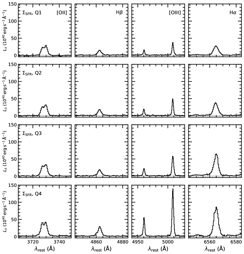
Figure 9.— Composite spectra constructed from the rest-frame optical MOSFIRE spectra of individual galaxies in the four bins of $\Sigma_{\rm SFR}$, from the lowest (top row) to highest bin (bottom row) of $\Sigma_{\rm SFR}$. Wavelength regions around [O II], H$\beta$, [O III], and H$\alpha$ are shown from the leftmost to rightmost column, respectively.

References

- Asplund et al. (2009) Asplund, M., Grevesse, N., Sauval, A. J., & Scott, P. 2009, ARA&A, 47, 481
- Azadi et al. (2017) Azadi, M., Coil, A. L., Aird, J., et al. 2017, ApJ, 835, 27
- Azadi et al. (2018) Azadi, M., Coil, A., Aird, J., et al. 2018, ApJ, 866, 63
- Bian et al. (2016) Bian, F., Kewley, L. J., Dopita, M. A., & Juneau, S. 2016, ApJ, 822, 62
- Bouwens et al. (2016) Bouwens, R. J., Smit, R., Labbé, I., et al. 2016, ApJ, 831, 176
- Brinchmann et al. (2008) Brinchmann, J., Pettini, M., & Charlot, S. 2008, MNRAS, 385, 769
- Calzetti et al. (2000) Calzetti, D., Armus, L., Bohlin, R. C., et al. 2000, ApJ, 533, 682
- Cardelli et al. (1989) Cardelli, J. A., Clayton, G. C., & Mathis, J. S. 1989, ApJ, 345, 245
- Chabrier (2003) Chabrier, G. 2003, PASP, 115, 763