On Robust Numerical Solver for ODE via Self-Attention Mechanism

Abstract

With the development of deep learning techniques, AI-enhanced numerical solvers are expected to become a new paradigm for solving differential equations due to their versatility and effectiveness in alleviating the accuracy-speed trade-off in traditional numerical solvers. However, this paradigm still inevitably requires a large amount of high-quality data, whose acquisition is often very expensive in natural science and engineering problems. Therefore, in this paper, we explore training efficient and robust AI-enhanced numerical solvers with a small data size by mitigating intrinsic noise disturbances. We first analyze the ability of the self-attention mechanism to regulate noise in supervised learning and then propose a simple-yet-effective numerical solver, AttSolver, which introduces an additive self-attention mechanism to the numerical solution of differential equations based on the dynamical system perspective of the residual neural network. Our results on benchmarks, ranging from high-dimensional problems to chaotic systems, demonstrate the effectiveness of AttSolver in generally improving the performance of existing traditional numerical solvers without any elaborated model crafting. Finally, we analyze the convergence, generalization, and robustness of the proposed method experimentally and theoretically.

1 Introduction

Mathematical models, represented by differential equations, are widely used in tackling various natural science and engineering problems, such as weather forecasting (Touma et al., 2021), transportation networks (Saberi et al., 2020), power grid management (Gholami & Sun, 2022), drug discovery (Aulin et al., 2021), etc. Effective solutions to these mathematical models can help researchers investigate and analyze the evolution process of the research objects to predict their future states. Those solutions are mainly obtained by specific numerical solvers, such as the Euler method (Shampine, 2018), Runge-Kutta method (Butcher, 2016), etc., which discretizes the solution space with a sufficiently fine step size and then performs numerical integration to achieve the solution. However, these classic numerical solvers encounter a trade-off between computation speed and solution accuracy. As the step size becomes smaller (finer), the accuracy is higher while the solution speed slows down; when the step size becomes larger (coarser), the solution speed increases, but the accuracy decreases.

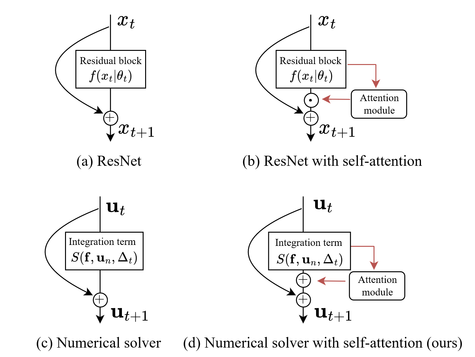
Figure 1: The comparison of (a) ResNet and (c) traditional forward numerical solver. (d) is a numerical solver with the self-attention mechanism (ours) inspired by the structure of (b) ResNet with self-attention. $\odot$ denotes the element-wise multiplication and $\oplus$ denotes the addition operator. Different from the common practice that multiple the output of the attention module to $f\left(x_{t}\mid\theta_{t}\right)$ in (b), we instead add the output of the attention module to $S\left(\mathbf{f},\mathbf{u}_{n},\Delta t\right)$ in (d), based on the optimization and error analysis in Section 6.

Confronted with this predicament, many recent works (Karniadakis et al., 2021; Li et al., 2020; Liang et al., 2022; Choudhary et al., 2020) on solving differential equations have introduced AI techniques, i.e., using data-driven neural networks to fit and replace differential operators or functions in the equations. Under the acceleration of GPU and the excellent approximation ability of neural networks, these works start to balance the speed and accuracy of solving differential equations. Although AI technology has achieved excellent results in solving differential equations, the versatility of these purely data-driven methods (PDDM) is still limited due to the inherent characteristics (Wang et al., 2022b) of differential equations and neural networks. Specifically, some differential equations are chaotic (Greydanus et al., 2019), i.e. sensitive to the initial values of inputs, which is hard for PDDM to fundamentally model the ubiquitous and elusive randomness of chaos with only finite data, leading to poor generalization (Abu-Mostafa et al., 2012); some differential equations are stiff (non-smooth) (Liang et al., 2022), and their solutions may undergo drastic changes in a very short time interval, which pose a great challenge for PDDM to handle stiff problems since neural networks tend to approximate smooth functions (Xu et al., 2020; Cao et al., 2019) intrinsically. To reduce this interference, a paradigm that shifts from “neural network replacement” to “neural network enhancement” has been recently proposed in (Huang et al., 2022b) called NeurVec, which uses neural networks to compensate for the errors generated by numerical solvers in the coarse step size $\Delta t_{c}$. Specifically, for the differential equation $\text{d}\mathbf{u}/\text{d}t=\mathbf{f}(\mathbf{u}),\mathbf{u}(0)=\mathbf{c}_{0}$, the forward numerical method of such a paradigm is

$$\mathbf{u}_{n+1}=\mathbf{u}_{n}+\underbrace{S(\mathbf{f},\mathbf{u}_{n},\Delta t_{c})\Delta t_{c}}_{\text{Integration term}}+\underbrace{\text{Net}(\mathbf{u}_{n}|\mathbf{\phi},\mathbb{D}_{f})}_{\text{Compensation term}},$$ (1)

where $\text{Net}(\cdot)$ is a neural network, $S(\cdot)$ is a numerical integration scheme, $\phi$ is the learnable parameters, $\mathbb{D}_{f}$ denotes the high-quality data, e.g. high-precision observation data or synthetic data generated by fine step size $\Delta t_{f}$. With suitable coarser step size $\Delta t_{c}$, the computation speed increases while the Eq.(1) still achieves high accuracy through the compensation term trained by $\mathbb{D}_{f}$, which alleviates the accuracy-speed trade-off in traditional numerical solvers. More details are introduced in Section 2.1. Compared to PDDM, this new paradigm can largely exploit the stability advantages of pure mathematical methods, given their physical correctness, to alleviate instability problems from chaos and stiffness. At the same time, it can enjoy the computation speedup as an AI-enhanced numerical solver.

However, since the prediction of the compensation term is achieved through deep learning, this new paradigm still inevitably requires numerous high-quality training data to ensure the prediction accuracy of the compensation term. Moreover, since most differential equations that require numerical solutions do not have analytical solutions, those high-quality data can only be observed or generated by investing a lot of labor and equipment costs. These nonnegligible costs hinder the implementation of the new paradigm. To this end, we ask a critical question:

Is it possible to train an efficient and robust AI-enhanced numerical solver with a small amount of data?

To answer this question, we explore the feasibility of obtaining AI-enhanced numerical solvers using a small amount of data, both empirically and theoretically in this paper. For this more realistic setting, due to the intrinsic differences between the obtained (observed or generated) training data and their corresponding ground truth, the inherent noise in the obtained data will readily hurt model training, especially when the data size is small (see Section 2.3 for details). This points out the main challenge of this critical setting, i.e., alleviating the adverse impact of the naturally existing noise in the training of the predictor of the compensation term.

To this end, we first analyze the noise issue faced by AI-enhanced numerical solvers training with a small amount of data. Then we correspondingly analyze the role of self-attention mechanisms in noise regulation (Liang et al., 2020; Zuo et al., 2022) in general supervised deep learning. Based on the dynamic system view (Weinan, 2017; Lu et al., 2018; Chang et al., 2017) of residual neural networks, we introduce self-attention mechanisms into the numerical solver, adapt the self-attention mechanisms based on the analysis and insights of numerical errors, and propose a simple-yet-effective novel numerical solver, AttSolver. Extensive experiments conducted on three benchmarks, i.e., a high-dimensional problem and chaotic systems demonstrate the effectiveness of AttSolver in generally improving the performance of existing traditional numerical solvers without any elaborated model crafting. Finally, we analyze the convergence, generalization, and robustness of the proposed method experimentally or theoretically. We summarize our contributions as follows:

• To the best of our knowledge, our proposed AttSolver is the first to introduce self-attention mechanisms into numerical solvers for differential equations. With a small amount of data, experiments on high-dimensional and chaotic systems show that our method can still effectively enhance multiple traditional numerical solvers.

• We also analyze the limitations and provide experimental or theoretical evidence for the convergence, generalization, and robustness of the proposed AttSolver.

2 Preliminaries

2.1 AI-enhanced numerical solver

As mentioned in Section 1, for ordinary differential equation $\text{d}\mathbf{u}/\text{d}t=\mathbf{f}(\mathbf{u}),\mathbf{u}(0)=\mathbf{c}_{0}$, we can obtain a numerical solution by a forward numerical solver (Butcher, 2016; Ames, 2014) given by the iterative formula

$$\mathbf{u}_{n+1}=\mathbf{u}_{n}+S(\mathbf{f},\mathbf{u}_{n},\Delta t)\Delta t,\quad\mathbf{u}_{0}=\mathbf{c}_{0}.$$ (2)

e.g., for the Euler method (Shampine, 2018), we have $S(\mathbf{f},\mathbf{u}_{n},\Delta t)\Delta t=\mathbf{f}(\mathbf{u}_{n})\Delta t$, where $\Delta t$ is a given step size, and $\mathbf{u}_{n}\in\mathbb{R}^{d}$ is an approximated solution at time $\sum_{i=0}^{n}\Delta t$. As shown in Eq.(1), the main idea of the AI-enhanced numerical solver is to use a neural network $\text{Net}(\mathbf{u}_{n}|\mathbf{\phi},\mathbb{D}_{f})$ as a corrector to compensate for the error of the integration term $S(\mathbf{f},\mathbf{u}_{n},\Delta t_{c})\Delta t_{c}$ with the coarse step size $\Delta t_{c}$. Compared to PDDM, this method has good acceleration while maintaining numerical accuracy. For example, if $\mathbb{D}_{f}$ is synthetic data generated by a fine step size $\Delta t_{f}$, then theoretically its evaluation speed is $\mathcal{O}(\frac{\Delta t_{c}}{(1+\epsilon)\Delta t_{f}})$ times (Huang et al., 2022b) that of the traditional method Eq.(2), where $\epsilon>0$ is related to the inference speed of the neural network.

2.2 The dynamical system view of residual block

The residual block structure has been successfully applied to many well-known neural network architectures, e.g., ResNet (He et al., 2016), UNet (Ronneberger et al., 2015), Transformer (Liu et al., 2021). As shown in Fig.1(a), the residual blocks in one stage can be written as

$$x_{t+1}=x_{t}+f(x_{t};\theta_{t}),$$ (3)

where $x_{t}\in\mathbb{R}^{d}$ is the input of neural network $f(\cdot;\theta_{t})$ with the learnable parameters $\theta_{t}$ in $t^{\rm th}$ block . Several recent studies (Weinan, 2017; Queiruga et al., 2020; Zhu et al., 2022; Meunier et al., 2022) have uncovered valuable connections between residual blocks and dynamic systems. i.e., the residual blocks can be interpreted as one step of forward numerical methods in Eq.(2) and Fig.1(c). The initial condition $\mathbf{u}_{0}=\mathbf{c}_{0}$ corresponds to the initial input $x_{0}$ of the network, and $\mathbf{u}_{t}$ corresponds to the input feature $x_{t}$ in $t^{\rm th}$ block. The output of neural network $f(\cdot;\theta_{t})$ in $t^{\rm th}$ block can be regarded as an integration $S(\mathbf{u}_{t};\mathbf{f},\Delta t)$ with step size $\Delta t$ and numerical integration scheme $S$. Given the above connection, some dynamical system theories (Chang et al., 2017; Chen et al., 2018) can be transferred to the analysis of residual neural networks, and more efficient neural network structures or deep learning applications (Huang et al., 2022a; Lu et al., 2018) can be designed.

2.3 The inherent noise in data

The high-quality data required by AI-enhanced numerical solvers inevitably have inherent noise in their acquisition process. On the one hand, the error in the observed data can come from the error of the measuring instruments. Theories like the uncertainty principle (Busch et al., 2007) also reveals the difficulty of collecting high-precision observation data. On the other hand, synthetic data, the other primary data acquisition method, inherently contains noise during their generation. Concretely, the choice of the numerical integration scheme $S$ in Eq.(2) and the data storage strategy both cause unavoidable losses on the accuracy of the synthesized data and hence introduce noise naturally. Last but not least, in many specific problems, we can only obtain the data by experiments. In this process, the objective noise may exhibit passively interfering with the data, such as interference from some unknown electromagnetic waves (Yao et al., 2021) or intermittent vibrations from the nearby subway (Wang et al., 2022a), etc.

3 Method

Inherent noise in the data tends to have an adverse effect on training neural networks, and learning with noisy data generally increases the training loss (Song et al., 2022). Such an effect will be more pronounced when the data size is limited (Abu-Mostafa et al., 2012). Additionally, for many complex differential equations, small noise can easily be accumulated and amplified in the iterative solving process of Eq.(1) or Eq.(2) due to chaotic issues (Huang et al., 2022b), leading to numerical explosions. As mentioned in Section 2.3, since these noises are almost inevitable, we need to regulate the noise to relieve their adverse impact. It should be noted that for the network used in general supervised learning tasks, such as a residual neural network in Fig.1(a), the noise in the training data, e.g., the batch noise introduced by batch training (Liang et al., 2020), can be regulated by adding a self-attention module, e.g., Fig.1(b). Now we provide the Theorem 3.1 as the theoretical evidence to justify the effect of the self-attention mechanism as a noise regulator.

Theorem 3.1.

Consider a $L$ layers residual neural network with self-attention module $Q(\cdot)$, i.e., $x_{t+1}=x_{t}+f(x_{t};W_{t})\odot Q[f(x_{t};W_{t})]$, $t=0,1,...,L-1$. And there exists a constant $r$ s.t. $\max\{|x_{t}\odot\nabla_{x}Q|\}\leq r$. Let $\epsilon$ be the perturbation from the noise and satisfies $\|x_{0}^{\epsilon}-x_{0}\|=\epsilon$, and $\epsilon_{t}=\|x_{t}^{\epsilon}-x_{t}\|$, we have

$$\epsilon_{t+1}\leq\epsilon_{t}\left(1+(\max\{Q[f(x_{t};W_{t})]\}+r)\|W_{t}\|_{2}\right),$$ (4)

where $\max$ refers to the largest element in a vector.

Proof.

(See Appendix B).∎

Theorem 3.1 reveals the principle of the self-attention mechanism on regulating the noise. Given an input $x_{0}$ and a perturbation $\epsilon$, we consider the noise input $x_{0}^{\epsilon}$ satisfied $x_{0}^{\epsilon}\in\{x|\|x-x_{0}\|=\epsilon\}$. According to Eq.(4), for a $L$ layers ResNet, the noise impact is $\epsilon_{L}=\|x_{L}^{\epsilon}-x_{L}\|$ and

$$\epsilon_{L}=\|x_{L}^{\epsilon}-x_{L}\| \leq\epsilon_{L-1}\left(1+\bar{Q}(x_{L-1})\|W_{L-1}\|_{2}\right)$$ (5)

$$\leq\epsilon\prod_{t=1}^{L-1}\left(1+\|W_{t}\|_{2}\bar{Q}(x_{t})\right)$$

where $\bar{Q}(x_{t})=\max\{Q[f(x_{t};W_{t})]\}+r$ depends on the self-attention term $Q[f(x_{t};W_{t})]$. Since $\|W_{t}\|_{2}\bar{Q}(x_{t})\geq 0$, the upper bound of the noise impact $\epsilon_{L}$ in Eq.(5) will be large if the number of layers $L$ is large. Thus the noise $\epsilon$ will have a pivotal impact on the network’s final output, especially in a deep network. In this case, the self-attention mechanism can change $\bar{Q}(x_{t})$ to adaptively control the upper bound $\epsilon\prod_{t=1}^{L-1}\left(1+\|W_{t}\|_{2}\bar{Q}(x_{t})\right)$. Note that generally, $\bar{Q}(x_{t})$ will not converge to 0 to obtain the minimum upper bound, i.e. $\epsilon$, since appropriate noise can enhance the robustness of the network and improve the generalization (Zhang et al., 2017; Cao et al., 2020). Moreover, if $\bar{Q}(x_{t})\to 0$, the forward process will degenerate to $x_{t+1}=x_{t}$, which may affect the representation learning of the network.

3.1 AttSolver: AI-enhanced Numerical Solver with Additive Self-Attention

Following the dynamical system view of residual block, in this section, we consider introducing self-attention mechanisms into numerical solvers to regulate the inherent noise when training with limited data, and propose a simple-yet-effective AI-enhanced numerical solver AttSolver, which is shown in Algorithm 1 and Fig.1(d).

Algorithm 1 The processing of AttSolver.

Input: A coarse step size $\Delta t_{c}$; The number of step $N$ which satisfied the evaluation time $T=N\Delta t_{c}$; A given equation $\text{d}\mathbf{u}/\text{d}t=\mathbf{f}(\mathbf{u}),\mathbf{u}(0)=\mathbf{c}_{0}$; A given numerical integration scheme $S$; The high-quality dataset $\mathbb{D}(\text{traj}(\mathbf{u}))$. The self-attention module $Q[\cdot|\phi]$; The learning rate $\eta$.

Output: The learned self-attention module $Q[\cdot|\phi]$.

epoch from 0 to Total epoch Estimate the trajectories Sample $\mathbf{u}=[\mathbf{u}_{0},\mathbf{u}_{1},...,\mathbf{u}_{N}]\sim\mathbb{D}(\text{traj}(\mathbf{u}))$; $\hat{\mathbf{u}}_{0}\leftarrow\mathbf{u}_{0}$; $t$ from 0 to $N-1$

Calculate integration term $\hat{S}\leftarrow S(\mathbf{f},\mathbf{u}_{t},\Delta t_{c})$;

Calculate self-attention term $Q[\hat{S}|\phi]$;

Estimate $\hat{\mathbf{u}}_{t+1}$ by Eq.(6);

Update the self-attention module $\hat{\mathbf{u}}\leftarrow[\hat{\mathbf{u}}_{1},...,\hat{\mathbf{u}}_{N}]$; Calculate the loss $R_{e}$ by Eq.(7); Update the parameters $\phi$ by $\phi\leftarrow\phi-\eta\nabla_{\phi}R_{e}$;

the self-attention module $Q[\cdot|\phi]$

The main iterative formula of AttSolver is defined as Eq.(6), and we highlight the additive self-attention with red color.

$$\hat{\mathbf{u}}_{n+1}=\hat{\mathbf{u}}_{n}+\hat{S}\Delta t_{c}{\color[rgb]{1,0,0}+Q[\hat{S}|\phi]},$$ (6)

where $\hat{S}=S(\mathbf{f},\hat{\mathbf{u}}_{n},\Delta t_{c})$ and $\phi$ is the learnable parameters of self-attention module. For estimated trajectory $\hat{\mathbf{u}}=[\hat{\mathbf{u}}_{1},...,\hat{\mathbf{u}}_{N}]$ and the ground truth trajectory from the high-quality dataset $\mathbb{D}(\text{traj}(\mathbf{u}))$, the loss $R_{e}$ can be defined as

$$R_{e}=c_{n}\cdot\frac{1}{N}\|\hat{\mathbf{u}}-\mathbf{u}\|_{2}^{2},$$ (7)

where $c_{n}$ is a constant which can alleviate the problem that the value of $R_{e}$ is too small due to the magnitude of $\mathbf{u}$ in some specific differential equations being too small. At this time, the gradient will be small enough and affect the optimization of the learnable parameter $\phi$. Compared with Eq.(1), $\text{Net}(\mathbf{u}_{n}|\mathbf{\phi},\mathbb{D}_{f})$ is replaced by a self-attention term $Q[\hat{S}|\phi]$. Note that according to the self-attention mechanism shown in Theorem 3.1, the self-attention term should be multiplicative, i.e., Eq.(6) can be rewritten as

$$\hat{\mathbf{u}}_{n+1}=\hat{\mathbf{u}}_{n}+\hat{S}\Delta t_{c}{\color[rgb]{0,0,1}\odot Q[\hat{S}|\phi]}.$$ (8)

In Section 6. we will discuss the reasons why we should use additive rather than multiplicative self-attention mechanisms for AI-enhanced numerical solvers in two-fold: (1) The multiplicative attention will interfere with the step size, leading to an unstable solution; (2) Eq.(8) will bring negative impacts on the optimization of the self-attention module. For $\hat{S}\in\mathbb{R}^{d}$, the architecture of self-attention module is

$$Q[\hat{S}|\phi]=\mathbf{W_{h}}\circ\mathbf{a}\circ\cdots\circ\mathbf{W_{2}}\circ\mathbf{a}\circ\mathbf{W_{1}}[\hat{S}],$$ (9)

where $\mathbf{a}$ is rational activation function (Boullé et al., 2020); $\mathbf{W_{i}},i$=$2,\cdots,h-1$ are $d_{1}\times d_{1}$ matrices, $\mathbf{W_{h}}\in\mathbb{R}^{d\times d_{1}}$ and $\mathbf{W_{1}}\in\mathbb{R}^{d_{1}\times d}$. We set $d_{1}=1024$ and $h=2$ by default.

Table 1: AttSolver for four forward numerical solvers on the spring-mass system with different dimensions. NeurVec is the state-of-the-art AI-enhanced Numerical solver. “data↓ 50%” denotes that we reduce the amount of training data by 50%. Red color means the accuracy of AttSolver can be improved with the SOTA method, and conversely, we use Green color.

	Numerical Solver	Enhanced Method	data↓ 50%	data↓ 75%	data↓ 90%
Spring-mass ($d=20$)	Euler	NeurVec	1.91e-1	2.12e-1	3.46e-1
	Euler	AttSolver	1.91e-1 ($\sim$0.0% )	2.12e-1 ($\sim$0.0% )	3.08e-1 ($\uparrow$ 10.98%)
	Improved Euler	NeurVec	4.76e-3	5.31e-3	7.45e-3
	Improved Euler	AttSolver	4.15e-3 ($\uparrow$ 12.81%)	4.78e-3 ($\uparrow$ 10.11%)	5.28e-3 ($\uparrow$ 29.11%)
	3rd order Runge-Kutta	NeurVec	2.47e-7	1.43e-6	2.63e-4
	3rd order Runge-Kutta	AttSolver	1.68e-7 ($\uparrow$ 31.95%)	2.37e-7 ($\uparrow$ 83.49%)	3.68e-5 ($\uparrow$ 86.01%)
	4th order Runge-Kutta	NeurVec	4.89e-8	1.48e-7	1.03e-5
	4th order Runge-Kutta	AttSolver	2.88e-8 ($\uparrow$ 41.11%)	4.33e-8 ($\uparrow$ 70.63%)	1.68e-6 ($\uparrow$ 83.89%)
Spring-mass ($d=50$)	Euler	NeurVec	1.32e-0	1.69e-0	2.90e-0
	Euler	AttSolver	1.32e-0 ($\sim$0.0% )	1.53e-0 ($\uparrow$ 9.29%)	2.03e-0 ($\uparrow$ 30.03%)
	Improved Euler	NeurVec	7.32e-2	1.45e-1	2.17e-1
	Improved Euler	AttSolver	5.43e-2 ($\uparrow$ 25.81%)	7.46e-2 ($\uparrow$ 48.40%)	9.73e-2 ($\uparrow$ 55.16%)
	3rd order Runge-Kutta	NeurVec	3.56e-6	5.03e-6	4.13e-4
	3rd order Runge-Kutta	AttSolver	2.27e-6 ($\uparrow$ 36.23%)	3.57e-6 ($\uparrow$ 29.15%)	4.32e-5 ($\uparrow$ 89.54%)
	4th order Runge-Kutta	NeurVec	6.44e-7	1.78e-6	4.03e-5
	4th order Runge-Kutta	AttSolver	3.84e-7 ($\uparrow$ 40.37%)	6.55e-7 ($\uparrow$ 63.20%)	5.68e-6 ($\uparrow$ 85.91%)
Spring-mass ($d=150$)	Euler	NeurVec	6.12e-0	1.54e1	9.11e1
	Euler	AttSolver	6.12e-0 ($\sim$0.0% )	1.32e1 ($\uparrow$ 14.29%)	7.12e1 ($\uparrow$ 21.84%)
	Improved Euler	NeurVec	2.49e-1	4.87e-1	2.76e-0
	Improved Euler	AttSolver	1.95e-1 ($\uparrow$ 21.87%)	3.04e-1 ($\uparrow$ 37.58%)	8.31e-1 ($\uparrow$ 69.89%)
	3rd order Runge-Kutta	NeurVec	4.87e-5	6.47e-5	8.34e-4
	3rd order Runge-Kutta	AttSolver	2.86e-5 ($\uparrow$ 41.27%)	3.32e-5 ($\uparrow$ 48.69%)	6.54e-5 ($\uparrow$ 92.16%)
	4th order Runge-Kutta	NeurVec	6.45e-6	1.56e-5	2.77e-4
	4th order Runge-Kutta	AttSolver	2.58e-6 ($\uparrow$ 60.05%)	4.78e-6 ($\uparrow$ 69.36%)	1.47e-5 ($\uparrow$ 94.69%)

Next, we take AttSolver with step size $k\Delta t$ and the Euler method as an example, and provide the convergence analysis for AttSolver in Theorem 3.2.

Theorem 3.2.

We consider ODE $\text{d}\mathbf{u}/\text{d}t=\mathbf{f}(\mathbf{u}),\mathbf{u}(0)=\mathbf{c}_{0}$ and Euler method $\mathbf{u}_{n+1}=\mathbf{u}_{n}+\Delta t\mathbf{f}(\mathbf{u}_{n})$ . We assume that (1) $\mathbf{f}$ is Lipschitz continuous with Lipschitz constant $L$ and (2) the second derivative of the true solution $\mathbf{u}$ is uniformly bounded by $M>0$, i.e., $\|\mathbf{u}^{\prime\prime}\|_{\infty}\leq M$ on $[0,T]$. Moreover, we assume that the attention module in AttSolver is Lipschitz continuous with Lipschitz constant $k\Delta tL_{\text{att}}$. For the solution of AttSolver $\hat{\mathbf{u}}$ with step size $k\Delta t$, we have

$$|\hat{\mathbf{u}}_{N}-\mathbf{u}(T)|\leq\alpha\Delta t+\beta\sqrt{\delta},$$ (10)

where $\alpha=\frac{1}{2L}M\exp(2TL)$, $\beta=\frac{\sqrt{T}\exp(TL(1+L_{\text{att}})}{\sqrt{L(1+L_{\text{att}})}}$ and $\delta$ is a error term about the training loss $R_{e}$. If the AttSlover can fit the training data well, i.e., $R_{e}\to 0$, the error $\delta\to 0$.

Proof.

(See Appendix C).∎

Previous works (Du et al., 2019; Jacot et al., 2018) based on neural tangent kernel theory reveal that under certain mild conditions, gradient descent allows a neural network to converge to a globally optimal solution, where the loss $R_{e}$ in Eq.(7) tends to 0. Then according to Theorem 3.2, we have $\delta\to 0$, and thus $|\hat{\mathbf{u}}_{N}-\mathbf{u}(T)|=\mathcal{O}(\Delta t)$. In this case, the AttSolver with step size $k\Delta t$ can achieve the same accuracy as the Euler method with the step size $\Delta t$, whose global truncation error is also $\mathcal{O}(\Delta t)$ (Butcher, 2016). However, the evaluation speed of AttSolver is approximately $\mathcal{O}(k)$ times greater than that of the Euler method in this situation.

4 Experiment

In this section, we consider two perspectives to verify the effectiveness of AttSolver: (1) on different numerical solvers and (2) different differential equation benchmarks. Specifically, since AttSolver is an AI-enhanced method for numerical solvers, we use many commonly used forward numerical solvers as backbones to evaluate the enhancement achieved by AttSolver, including the Euler method, Improved Euler method, 3rd and 4th order Runge-Kutta methods (see Appendix A for details.). On the other hand, to demonstrate that AttSolver is competent for complex differential equations, we further experiment on two chaotic dynamical systems on the 4th order Runge-Kutta method, i.e., k-link pendulum and elastic pendulum. For all experiments in this section, for fair comparisons, we follow the settings in (Huang et al., 2022b; Chen et al., 2020) for all generations of initial conditions and metrics. We elaborate on the rationale of choosing comparison methods in Appendix A.

4.1 AttSolver for different numerical solvers

In this section, we consider a high-dimensional linear system, namely the spring-mass system, and four forward numerical solvers (the details of these solvers can be found in Appendix A). In a spring-mass system, there are $d$ masses and $d+1$ springs connecting in sequence, and they are placed horizontally with two ends connected to two fixed blocks. The corresponding ODE of this system is

$$\small\frac{\text{d}}{\text{d}t}\left(\begin{array}[]{l}q_{i}\\ p_{i}\end{array}\right)=\left(\begin{array}[]{l}p_{i}/m\\ k_{i}\left(q_{i-1}-q_{i}\right)+k_{i+1}\left(q_{i+1}-q_{i}\right)\end{array}\right),$$ (11)

$i=1,2,\cdots,d,q_{0}=q_{d+1}=0$, where $m_{i}$ and $k_{i}$ are the mass of the $i^{\rm th}$ mass and force coefficient of the $i^{\rm th}$ spring, respectively. The momentum and the position of $i^{\rm th}$ mass are denoted as $p_{i}$ and $q_{i}$. We adopt the coarse step size $\Delta t=2e-1$ for the numerical solver and the fine step size $1e-3$ for training the enhanced method.

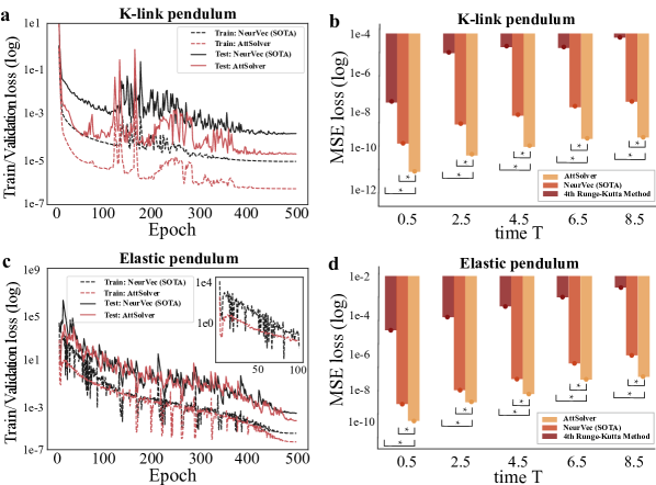
Figure 2: The simulation on different chaotic systems with step size $1e-1$. a and c are the train/validation loss curves; b and d is the Mean Squared Error (MSE) loss on the test set. The significance level $\alpha$ is 0.05. Notation: “*”: $p<0.05$.

The experiment results at evaluation time $T=20$ are shown in Table 1. For the Euler method with low simulation accuracy, our AttSolver achieves consistent performance with the state-of-the-art (SOTA) enhanced method, i.e., NeurVec (Huang et al., 2022b), for the spring-mass system in different dimensions. For other numerical solvers with higher accuracy, AttSolver can better enhance the solver than NeurVec. Even for the spring-mass system with increasing dimensions, although the difficulty of the simulation increases, AttSolver can still maintain the performance. In addition, we can observe that our AttSolver can achieve similar performance as the SOTA method with less data size , showing that we are capable of training an efficient and robust AI-enhanced numerical solver with a small amount of data. In fact, such performance improvements as in Table 1 are meaningful and significant, and as mentioned in Section 3, small errors can easily be accumulated and amplified in the iterative solving process. We will give a corresponding example of the numerical explosion in Section 6 (Fig.3).

4.2 AttSolver for different systems

Table 2: The impact of the depth $h$ and width $d_{1}$ of the self-attention module on the simulation performance. Rel. Infe. Speed is the relative inference speed of the network based on our proposed AttSolver setting, i.e., $h=2$ and $d_{1}=1024$.

	Spring-mass		$K$-link pendulum		Elastic pendulum
	MSE loss	Rel. Infe. Speed	MSE loss	Rel. Infe. Speed	MSE loss	Rel. Infe. Speed
$h=2$ (ours)	2.58e-6	-	4.26e-9	-	5.41e-7	-
$h=3$	2.49e-6 ($\uparrow$ 3.61%)	$\downarrow$ 88.49%	4.39e-9 ($\downarrow$ 2.52%)	$\downarrow$ 91.60%	5.28e-7 ($\uparrow$ 2.46%)	$\downarrow$ 90.89%
$h=4$	2.55e-6 ($\uparrow$ 1.18%)	$\downarrow$ 93.95%	4.42e-9 ($\downarrow$ 3.62%)	$\downarrow$ 95.64%	5.58e-7 ($\downarrow$ 3.05%)	$\downarrow$ 95.33%
$d_{1}=512$	3.76e-5 ($\downarrow$ 83.36%)	$\uparrow$ 27.59%	2.56e-8 ($\downarrow$ 93.14%)	$\uparrow$ 15.36%	2.56e-6 ($\downarrow$ 78.87%)	$\uparrow$ 17.25%
$d_{1}=1024$ (ours)	2.58e-6	-	4.26e-9	-	5.41e-7	-
$d_{1}=2048$	2.41e-6 ($\uparrow$ 7.05%)	$\downarrow$ 26.48%	3.98e-9 ($\uparrow$ 7.03%)	$\downarrow$ 23.12%	4.83e-7 ($\uparrow$ 12.01%)	$\downarrow$ 24.63%

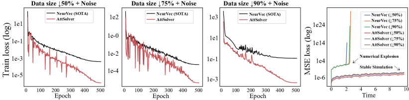
Figure 3: The noise attack experiments for the Elastic pendulum under different data sizes. AttSolver, with the self-attention mechanism, can better mitigate the adverse effects of noise than the SOTA method.

In this section, we reduce the amount of training data by 50% and use two chaotic dynamical systems to verify the effectiveness of our AttSolver, i.e., the Elastic and $K$-link pendulum. The Elastic pendulum considers a ball without volume connected to an elastic rod. Under the effect of gravity and force of spring (Breitenberger & Mueller, 1981), the motion of the ball will be chaotic, and its ODE is

$$\small\frac{\text{d}}{\text{d}t}\left(\begin{array}[]{l}\theta\\ r\\ \dot{\theta}\\ \dot{r}\\ \end{array}\right)=\left(\begin{array}[]{l}\dot{\theta}\\ \dot{r}\\ \frac{1}{r}(-g\sin\theta-\dot{\theta}\dot{r})\\ r\dot{\theta}^{2}-\frac{k}{m}(r-l_{0})+g\cos\theta\end{array}\right),$$ (12)

where $k,m,l_{0}$, and $g$ are related constants. There are two variables $\theta$ and $r$ in Eq.(12). Specifically, $r$ is the length of the spring, and $\theta$ is the angle between the spring and the vertical axis. For $K$-link pendulum, it considers $K$ balls connected end to end with $K$ rods under the effect of gravity (Lopes & Tenreiro Machado, 2017), and its ODE is

$$\text{d}(\mathbf{\theta},\dot{\mathbf{\theta}})/\text{d}t=(\dot{\mathbf{\theta}},\mathbf{A^{-1}}\mathbf{b}).$$ (13)

where $\mathbf{\theta}=(\theta_{1},\theta_{2},\cdots,\theta_{K})$ and $\theta_{i}$ is the angle between the $i^{\rm th}$ rod and the vertical axis. Let $\mathbf{b}=(b_{1},b_{2},\cdots,b_{K})$ and $b_{i}=-\sum_{j=1}^{K}\left[c(i,j)\dot{\theta}_{j}^{2}\sin\left(\theta_{i}-\theta_{j}\right)\right]-(K-i+1)g\sin\theta_{i}$. $\mathbf{A}$ is a $K\times K$ matrix and the element in $\mathbf{A}_{i,j}$ is $[K-\max(i,j)+1]\cos\left(\theta_{i}-\theta_{j}\right)$. The simulation results are shown in Fig.2. We first analyze the train/validation loss curves. For the $K$-link pendulum, AttSolver’s loss is significantly smaller than that of the SOTA method in both the training and validation phase. For the elastic pendulum, at the beginning of the training phase, AttSolver’s curve is smoother, and the loss is about 3$\sim$4 orders of magnitude better than NeurVec. As the epoch increases, the loss curves of AttSolver are similar to those of the SOTA method in both training and validation phases until about 400 epochs, and we can observe that AttSolver can converge in the local optimal point with a smaller loss. Next, for Fig.2b and 2d, AttSolver can significantly reduce the error of the traditional method, i.e., 4th order Runge-Kutta methods, under the same step size $1e-1$ in the test phase, indicating that it is feasible to compensate the error of the numerical solver by the self-attention mechanism. Moreover, at the significance level $\alpha=0.05$, our method has a smaller MSE loss and can still significantly outperform the SOTA method.

5 Ablation study

In this section, we perform several ablation studies on AttSolver. In Table 2, we analyze the impact of the depth $h$ and width $d_{1}$ for the self-attention module in Eq.(9). We observe that the depth $h$ has little effect on the MSE loss in all benchmarks, but the model’s performance is positively correlated with the width $d_{1}$. Therefore, to increase the inference speed, we choose a sufficiently shallow depth $h=2$ and appropriate width $d_{1}=1024$ for AttSolver.

Table 3: The impact of skip connection and considering $\Delta t_{c}$ as a part of the input.

Benchmark	w/ skip	w/o $\Delta t_{c}$	w/o $\Delta t_{c}$ & w/o skip (ours)
Spring-mass	4.57e-4 ($\downarrow$ 99.44%)	3.67e-6 ($\downarrow$ 29.78%)	2.58e-6
$K$-link pendulum	6.36e-6 ($\downarrow$ 99.93%)	4.18e-9 ($\uparrow$ 1.91%)	4.26e-9
Elastic pendulum	1.39e-4 ($\downarrow$ 99.61%)	1.65e-6 ($\downarrow$ 67.21%)	5.41e-7

Then we study popular residual structures for AttSolver. From Table 3, the skip connection will bring significant negative impacts on simulation for both high-dimension linear systems and chaotic dynamical systems. This motivates us to adopt a simple stacking structure like Eq.(9) for our AttSolver. Moreover, we analyze the form of the input of the self-attention module, where we take $\hat{S}$ as input instead of the complete integration term $\hat{S}\Delta t_{c}$ in Eq.(9). In Table 3, we show that the input $\hat{S}$ has better performance than input $\hat{S}\Delta t_{c}$, except for $K$-link pendulum (similar performance).

6 Discussion

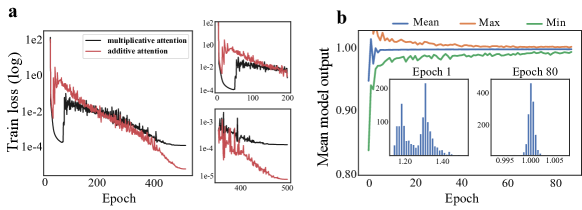
Figure 4: a. The loss curves for two kinds of attention. The loss minimization of multiplicative attention is fast at first and then slow during the last epochs, which have a local minimum with a large loss; b. The mean of attention value $Q[\hat{S}|\phi]$ (blue) while using Eq.(8), which quickly converges to the vicinity of constant 1 during training.

The robustness of AttSolver. Our proposed method AttSolver is inspired by the self-attention mechanism in ResNet, whose robustness is guaranteed by Theorem 3.1. In Fig.3, we empirically explore the robustness of AttSolver by noise attack experiments under different data sizes. Specifically, in the training process, we can interfere with the training phase of AttSolver by adding constant noise $\sigma=1e-5$ to $\hat{\mathbf{u}}_{n}$, i.e., $\hat{\mathbf{u}}_{n}\leftarrow\hat{\mathbf{u}}_{n}+\sigma$ for all $n$ in Eq.(6). Experimental results show that, compared with the SOTA method, our proposed method can significantly regulate the noise, leading to smaller training loss and stable simulations. In contrast, the SOTA method explodes numerically at the beginning of the simulation due to the effect of noise in all settings.

Why not multiplicative attention in AttSolver? Now we analyze the multiplicative attention in Eq.(8). In mathematics, multiplicative attention may incorrectly estimate the integration term $\hat{S}\Delta t_{c}\odot Q[\hat{S}|\phi]$ and cause an unstable solution. The reason is that the step size $\Delta t_{c}$ in $\hat{S}$ used for discretization is not equal to the step size $\Delta t_{c}^{\prime}:=\Delta t_{c}\odot Q[\hat{S}|\phi]$ used for integration under the multiplicative attention, unless $Q[\hat{S}|\phi]$ is a constant vector $\mathbf{I}$ whose elements are all 1. In fact, $Q[\hat{S}|\phi]$ does converge around $\mathbf{I}$, as shown in Fig.4b. From an optimization viewpoint, this is because, in Eq.(1), the AI-enhanced method aims to compensate for the errors of the traditional numerical solver, and hence the magnitude of the compensation term $\epsilon_{c}$ will be small. Then if multiplicative attention is used, we have

$$\hat{S}\Delta t_{c}+\epsilon_{c}=\hat{S}\Delta t_{c}\odot Q[\hat{S}|\phi],$$ (14)

i.e., $(Q[\hat{S}|\phi]-\mathbf{I})\hat{S}\Delta t_{c}=\epsilon_{c}$. Since $\hat{S}\Delta t_{c}\gg\epsilon_{c}$, we have $Q[\hat{S}|\phi]\approx\mathbf{I}$. This means the self-attention module will tend to fit a constant vector, which will bring negative impacts on its optimization (Wang et al., 2022b), like Fig.4a. To mitigate this issue, a simple-yet-effective strategy is to normalize the attention as $\mathbf{I}+\widetilde{Q}[\hat{S}|\phi]$, and we rewrite Eq.(8)

$$\hat{\mathbf{u}}_{n+1} =\hat{\mathbf{u}}_{n}+\hat{S}\Delta t_{c}{\color[rgb]{0,0,1}\odot\left(\mathbf{I}+\widetilde{Q}[\hat{S}|\phi]\right)}$$ (15)

$$=\hat{\mathbf{u}}_{n}+\hat{S}\Delta t_{c}\underbrace{{\color[rgb]{1,0,0}+\hat{S}\Delta t_{c}\odot\widetilde{Q}[\hat{S}|\phi]}}_{\text{Additive attention}},$$

where the term $\hat{S}\Delta t_{c}\odot\widetilde{Q}[\hat{S}|\phi]$ can be regarded as the additive attention term for $\hat{\mathbf{u}}_{n}+\hat{S}\Delta t_{c}$ and Eq.(15) has the same form as Eq.(6). Therefore, for AttSolver, we adopt additive attention instead of multiplicative attention.

Limitations of AttSolver. From the experiment results in Section 4 and Section 5, the proposed AttSolver can achieve good enough simulation performance with less training data. However, AttSolver does not completely prevent the solution from being disturbed under the inherent noise in the dataset. So we aim to alleviate the noise issue rather than solve it completely. If we want to further mitigate this issue, we may need more elaborate network structures and training settings to enhance the effectiveness of our AttSolver.

Theorem 6.1.

We consider the SOTA method and AttSolver under the view of Vapnik-Chervonenkis theory (Vapnik, 1999). For $\epsilon>0$, when the data size is more than $N^{\prime}$, the empirical error of two methods satisfy $R_{e}(\phi|\text{Neur.})\leq\epsilon$ and $R_{e}(\phi|\text{Att.})\leq\epsilon$. For small enough $\epsilon_{0}\ll\epsilon$ and Euler method, we have

$$N(\text{Att.})\lesssim N(\text{Neur.}),$$ (16)

where $N(*)$ is the lower bound of the data size that the generalization error of method $*$ can reach $\epsilon(1-\epsilon_{0})^{-1}$.

Proof.

(See Appendix D).∎

Now we extend our discussion of the data size, where some analyses have been given by Theorem 6.1 under the Euler method and some mild assumptions. Compared to the SOTA method, AttSolver requires a smaller data size to achieve the same generalization error, which is consistent with the experimental results in Table 1. Although our proposed method does reduce the data size required by the SOTA method, the accuracy may not be sufficient for all the problems in the natural sciences and engineering. Therefore, if we need to solve a problem that requires high accuracy, it would be better to increase the training data size as much as possible to further improve the performance of the AI-enhance solver than only relying on the algorithmic design. This is because we can observe when the complete training data is used, the improvement brought by AttSolver may be less than 10%, which is reasonable since the AttSolver is designed tailored to the data-insufficient scenario and we have not explicitly maximized the performance of AttSolver when the data is sufficient. In the future, we will explore improving the AttSolver in the data-sufficient scenario.

7 Conclusion

This paper discusses how to train an effective and robust AI-enhanced numerical solver for differential equations with a small amount of data to alleviate the high data acquisition costs. Using the dynamical system view of ResNet, we introduce the self-attention mechanism into the numerical solver and propose AttSolver to mitigate the adverse effects of the inherent noise when the data is limited. Experimental results show the effectiveness of AttSolver in improving traditional numerical solvers with limited data, where we also analyze the convergence, generalization, and robustness.

Appendix A The details of the proposed algorithm.

On the rationale of choosing comparison methods. Existing frontier works on solving differential equations based on neural networks can be divided into “neural network replacement” and “neural network enhancement” methods.

The core idea of “neural network replacement” methods is to replace the role of the numerical solver in a data-driven manner. Different kinds of “neural network replacement” methods are differentiated by their replacement approaches. First, if a large amount of high-quality and uniformly sampled data is available, some specially structured neural networks (Wang et al., 2022b; Geneva & Zabaras, 2022; Liang et al., 2021) can directly approximate the integral curve such that it can replace the whole numerical solver without considering the physical properties of the equation. On the other hand, the PINN methods (Choudhary et al., 2020; Raissi et al., 2019; Ji et al., 2021; Cai et al., 2021) consider using sampling to replace the differential process while incorporating the physical information of the equations by constructing suitable loss functions. Last but not least, the operator-based methods focus on replacing the differential operators (Li et al., 2021; Lu et al., 2021) in a data-driven manner, where its basic idea is to approximate the solution operator by a neural network and replace the traditional solver during numerical simulations to improve the efficiency of the solution process.

Although the “neural network replacement” method has an excellent performance in solving many differential equations, these methods rely heavily on neural networks, so there are still some problems that cannot be easily overcome. For instance, The operator-based methods prefer certain solutions with clean boundary regions (Ji et al., 2021), and the fitting of operators is relatively sensitive to model initialization and structural design (Meng et al., 2022); The method of directly fitting the integral curve may ignore the effect of chaos or stiffness in the differential equation (Liang et al., 2022). Moreover, the PINN methods do not have versatility for the initial values of the equation and we need to be retrained (Zhong et al., 2022; Psaros et al., 2022; Wang et al., 2021) the network for different initial values, etc.

In contrast, the “neural network enhancement” method does not completely replace the numerical solver. Instead, it only leverages the neural network to augment the existing numerical solver (Huang et al., 2022b). Such a paradigm reduces the dependence on data-driven methods and ensures physical correctness since the traditional numerical solver still plays the main role in solving differential equations. Moreover, as most practical applications use the traditional solver paradigm as a primary choice, the “neural network enhancement” method has another advantage compared to the “neural network replacement” method in that we can directly integrate the enhancement method into the existing numerical solver system without changing any user’s habits or interrupting the deployed solver system.

Therefore, due to the difference in applicable scenarios and the scope of application between the paradigms of “neural network replacement” and “neural network enhancement”, in this paper, we primarily compare the method belonging to the “neural network enhancement” category, e.g., NeurVec (Huang et al., 2022b), to ensure an apple-to-apple comparison to avoid the unreasonable and even impossible apple-to-orange comparison.

Table 4: Summary of the datasets mentioned in this paper.

Benchmark	Type	Dimension	Data size	Step size	Generative Method	Evaluation time $T$
Spring-mass	Train	*	5k	1e-3	*	20
Spring-mass	Validation	*	0.1k	1e-5	RK4	20
Spring-mass	Test	*	5k	1e-5	RK4	20
2-link pendulum	Train	4	20k	1e-3	RK4	10
2-link pendulum	Validation	4	1k	1e-5	RK4	10
2-link pendulum	Test	4	10k	1e-5	RK4	10
Elastic pendulum	Train	4	20k	1e-3	RK4	50
Elastic pendulum	Validation	4	1k	1e-5	RK4	50
Elastic pendulum	Test	4	10k	1e-5	RK4	50

The details of dataset. We summarize the information on training, validation, and test data for all benchmarks in this paper in Table 4. We obtain the discrete solutions every step size up to the model time $T$ and the evaluation time for all experimental results of MSE loss in this paper is $T$. The Generative method of Spring-mass during training depends on the numerical solver used in Table 1. Moreover, the dimension of the Spring-mass system also depends on $d$ in Table 1, and if $d=20$, the dimension is $2d=40$. “RK4” denotes 4th order Runge-Kutta method.

Table 5: The initialization of different benchmarks. “Uniform random” means that the variables are sampled with uniform distribution of a given range. “Constant” means the variable is initialized as a constant. The dimension of $\mathbf{p}$ and $\mathbf{q}$ in Spring-mass system depends on $d$ in Table 1, and if $d=20$, their dimension are $d=20$.

Task	Variable	Dimension	Type	Range of initialization	Model input?
Spring-mass	$\mathbf{p}$	*	Uniform random	$[-2.5,2.5]^{20}$	✓
Spring-mass	$\mathbf{q}$	*	Uniform random	$[-2.5,2.5]^{20}$	✓
Elastic pendulum	$\theta$	1	Uniform random	$[0,\pi/8]$	✓
Elastic pendulum	$r$	1	Constant	10	✓
Elastic pendulum	$\dot{\theta}$	1	Constant	0	✓
Elastic pendulum	$\dot{r}$	1	Constant	0	✓
Elastic pendulum	$l_{0}$	1	Constant	10
Elastic pendulum	$g$	1	Constant	9.8
Elastic pendulum	$k$	1	Constant	40
Elastic pendulum	$m$	1	Constant	1
2-link pendulum	$\mathbf{\theta}$	2	Uniform random	$[0,\pi/8]^{2}$	✓
2-link pendulum	$\mathbf{\dot{\theta}}$	2	Constant	0	✓
2-link pendulum	$m$	1	Constant	1
2-link pendulum	$g$	1	Constant	9.8

Numerical solvers. In this paper, we consider four forward numerical solvers to validate the effectiveness of our proposed AttSolver, including the Euler method, Improved Euler method, 3rd and 4th order Runge-Kutta methods. In this section, we introduce these solvers. As mentioned in Eq.(2), these solvers have different integration terms $S(f,u_{n},\Delta t)$.

Table 6: The integration terms for different kinds of numerical solvers with step size $\Delta t$.

Numerical solver	Integration term $S(f,u_{n},\Delta t)$	Global truncation error
Euler	$\Delta t\mathbf{f}(\mathbf{u}_{n})$	$\mathcal{O}(\Delta t)$
Improved Euler	$\frac{\Delta t}{2}[\mathbf{f}(\mathbf{u}_{n})+\mathbf{f}(\mathbf{u}_{n}+\Delta t\mathbf{f}(\mathbf{u}_{n}))]$	$\mathcal{O}(\Delta t^{2})$
3rd order Runge-Kutta	$\Delta t(\lambda_{1}K_{1}+\lambda_{2}K_{2}+\lambda_{3}K_{3})$	$\mathcal{O}(\Delta t^{3})$
4th order Runge-Kutta	$\Delta t(\beta_{1}J_{1}+\beta_{2}J_{2}+\beta_{3}J_{3}+\beta_{4}J_{4})$	$\mathcal{O}(\Delta t^{4})$

For 3rd order Runge-Kutta method ,the coefficients $\lambda_{1}=\lambda_{3}=\frac{1}{6}$ and $\lambda_{2}=\frac{2}{3}$. Besides, $K_{1}=\mathbf{f}(\mathbf{u}_{n}),K_{2}=\mathbf{f}(\mathbf{u}_{n}+\frac{\Delta t}{2}K_{1})$ and $K_{3}=\mathbf{f}(\mathbf{u}_{n}-\Delta tK_{1}+2\Delta tK_{2})$. For the 4th order Runge-Kutta method, $\beta_{1}=\beta_{4}=\frac{1}{6}$ and $\beta_{2}=\beta_{3}=\frac{1}{3}$. Moreover, $J_{1}=\mathbf{f}(\mathbf{u}_{n}),J_{2}=\mathbf{f}(\mathbf{u}_{n}+\frac{\Delta t}{2}J_{1}),J_{3}=\mathbf{f}(\mathbf{u}_{n}+\frac{\Delta t}{2}J_{2})$ and $J_{4}=\mathbf{f}(\mathbf{u}_{n}+\Delta tJ_{3})$. Generally speaking, 4th order Runge-Kutta method has the smallest Global truncation error $\mathcal{O}(\Delta t^{4})$, i.e., 4th order Runge-Kutta method has the highest accuracy. However, due to its most complex integration term $\Delta t(\beta_{1}J_{1}+\beta_{2}J_{2}+\beta_{3}J_{3}+\beta_{4}J_{4})$, its simulation speed is the slowest among the four numerical solvers in Table 6.

Appendix B The proof of Theorem 3.1

Theorem 3.1. Consider a $L$ layers residual neural network with self-attention module $Q(\cdot)$, i.e., $x_{t+1}=x_{t}+f(x_{t};W_{t})\odot Q[f(x_{t};W_{t})]$, $t=0,1,...,L-1$. And there exists a constant $r$ s.t. $\max\{|x_{t}\odot\nabla_{x}Q|\}\leq r$. Let $\epsilon$ be the perturbation coming from noise and satisfies $\|x_{0}^{\epsilon}-x_{0}\|=\epsilon$, and $\epsilon_{t}=\|x_{t}^{\epsilon}-x_{t}\|$, we have

$$\epsilon_{t+1}\leq\epsilon_{t}\left(1+(\max\{Q[f(x_{t};W_{t})]\}+r)\|W_{t}\|_{2}\right),$$ (17)

where $\max$ refers to the largest element in a vector.

Proof.

Let $H(x)=f(x_{t};W_{t})\odot Q[f(x_{t};W_{t})]$, according to Taylor expansion, we have

$$H(x_{t}^{\epsilon})=H(x_{t})+(x_{t}^{\epsilon}-x_{t})^{T}\nabla_{x}H(x)|_{x=x_{t}}$$ (18)

For $\epsilon_{t+1}=\|x_{t+1}^{\epsilon}-x_{t+1}\|$, we have

$$\epsilon_{t+1} =\|x_{t+1}^{\epsilon}-x_{t+1}\|$$

$$=\|x_{t}^{\epsilon}+f(x_{t}^{\epsilon};W_{t})\odot Q[f(x_{t}^{\epsilon};W_{t})]-x_{t}-f(x_{t};W_{t})\odot Q[f(x_{t};W_{t})]\|$$

$$=\|(x_{t}^{\epsilon}-x_{t})+f(x_{t}^{\epsilon};W_{t})\odot Q[f(x_{t}^{\epsilon};W_{t})]-f(x_{t};W_{t})\odot Q[f(x_{t};W_{t})]\|$$

$$=\|(x_{t}^{\epsilon}-x_{t})+(x_{t}^{\epsilon}-x_{t})^{T}\nabla_{x}H(x)|_{x=x_{t}}\|$$ Since Eq.(18)

$$\leq\|(x_{t}^{\epsilon}-x_{t})\|\cdot(1+\|\nabla_{x}H(x)|_{x=x_{t}}\|) \|ab\|\leq\|a\|\|b\|$$ Since

$$=\epsilon_{t}(1+\|\nabla_{x}H(x)|_{x=x_{t}}\|)$$

Next, we analyze $\nabla_{x}H(x)|_{x=x_{t}}$. We also follow and consider the assumption (Yang et al., 2020) that $f(x_{t};W_{t})$ is consists of linear transformation and ReLU non-linear activation $\mathbf{A}$, i.e., $f(x_{t};W_{t})=\mathbf{A}W_{t}x_{t}$. Note that $\mathbf{A}$ is a diagonal matrix

$$\mathbf{A}=\begin{pmatrix}a_{1}&0&0&0\\ 0&a_{2}&0&0\\ 0&0&\ddots&0\\ 0&0&0&a_{d}\\ \end{pmatrix},\quad a_{1},a_{2},..,a_{d}\in\{0,1\},$$ (19)

where $d$ is dimension of $x_{t}$ and and each element $a_{i},i=1,2,...,d$ in $\mathbf{A}$ is 0 or 1. If the $i^{\rm th}$ element in $x_{t}$ is positive, the value of $a_{i}=1$, otherwise equals to zero. Therefore the 2-norm, i.e., the largest singular value, of $\mathbf{A}$ is less than 1, i.e.,

$$\|\mathbf{A}\|_{2}=\sqrt{\lambda_{\max}\mathbf{A}^{T}\mathbf{A}}=\sqrt{\lambda_{\max}\mathbf{A}}\leq 1$$ (20)

Hence, we can further estimate $\|\nabla_{x}H(x)|_{x=x_{t}}\|$ that

$$\|\nabla_{x}H(x)|_{x=x_{t}}\| =\|\nabla_{x}f(x;W_{t})|_{x=x_{t}}\odot Q[f(x_{t};W_{t})]+f(x_{t};W_{t})\odot\nabla_{x}Q|_{x=x_{t}}\|$$

$$\leq\|\mathbf{A}W_{t}\mathbf{I}\odot Q[f(x_{t};W_{t})]\|+\|\mathbf{A}W_{t}x_{t}\odot\nabla_{x}Q|_{x=x_{t}}\|$$

$$\leq\max\{Q[f(x_{t};W_{t})]\}\cdot\|\mathbf{A}\|\|W_{t}\|+r\cdot\|\mathbf{A}\|\|W_{t}\| \max\{|x_{t}\odot\nabla_{x}Q|\}\leq r$$ Since

$$\leq(\max\{Q[f(x_{t};W_{t})]\}+r)\|W_{t}\|$$ Since Eq.(20)

Therefore, we have $\epsilon_{t+1}\leq\epsilon_{t}\left(1+(\max\{Q[f(x_{t};W_{t})]\}+r)\|W_{t}\|_{2}\right)$.

∎

Appendix C The proof of Theorem 3.2

Theorem 3.2. We consider ODE $\text{d}\mathbf{u}/\text{d}t=\mathbf{f}(\mathbf{u}),\mathbf{u}(0)=\mathbf{c}_{0}$ and Euler method $\mathbf{u}_{n+1}=\mathbf{u}_{n}+\Delta t\mathbf{f}(\mathbf{u}_{n})$ . We assume that (1) $\mathbf{f}$ is Lipschitz continuous with Lipschitz constant $L$ and (2) the second derivative of the true solution $\mathbf{u}$ is uniformly bounded by $M>0$, i.e., $\|\mathbf{u}^{\prime\prime}\|_{\infty}\leq M$ on $[0,T]$. Moreover, we assume that the attention module in AttSolver is Lipschitz continuous with Lipschitz constant $k\Delta tL_{\text{att}}$. For the solution of AttSolver $\hat{\mathbf{u}}$ with step size $k\Delta t$, we have

$$|\hat{\mathbf{u}}_{N}-\mathbf{u}(T)|\leq\alpha\Delta t+\beta\sqrt{\delta},$$ (21)

where $\alpha=\frac{1}{2L}M\exp(2TL)$, $\beta=\frac{\sqrt{T}\exp(TL(1+L_{\text{att}})}{\sqrt{L(1+L_{\text{att}})}}$ and $\delta$ is a error term about the training of AttSlover. If the AttSlover can fit the training data well, the error $\delta\to 0$.

Lemma C.1.

If the assumptions (1) and (2) in Theorem 3.2 hold, for Euler method $\mathbf{u}_{n+1}=\mathbf{u}_{n}+\Delta t\mathbf{f}(\mathbf{u}_{n})$, we have

$$|\mathbf{u}_{Nk}-\mathbf{u}(T)|\leq\frac{M\exp(2TL)}{2L}\Delta t,$$ (22)

where $0=t_{0}<t_{1}<\cdots<t_{Nk}=T$ be uniform points on $[0,T]$ and $\Delta t=\frac{T}{Nk}$.

Lemma C.2.

For any $n\in\mathbb{N}_{+}$ and $x>0$, we have

$$(1+x)^{n}\leq\exp(nx),$$ (23)

Proof.

(For Lemma 23). According to the Taylor expansion, we have

$$\exp(nx)=\sum_{i=0}^{\infty}\frac{(nx)^{i}}{i!}\geq\sum_{i=0}^{\infty}n^{i}\frac{x^{i}}{i!}\geq\sum_{i=0}^{\infty}\prod_{j=0}^{i-1}(n-j)\frac{x^{i}}{i!}=\sum_{i=0}^{\infty}C_{n}^{i}x^{i}=(1+x)^{n}$$ (24)

∎

Proof.

(For Theorem 3.2.)

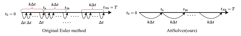
Figure 5: The discretization of the original Euler method (Left) and our AttSolver (Right).

Let’s consider the discretization for time interval $[0,T]$ as shown in Fig.5, and $E_{n}:=\hat{\mathbf{u}}_{n}-\mathbf{u}_{nk}$

$$|\hat{\mathbf{u}}_{Nk}-\mathbf{u}(T)| \leq|\mathbf{u}_{Nk}-\mathbf{u}(T)|+|\hat{\mathbf{u}}_{N}-\mathbf{u}_{Nk}| |a-b|\leq|a|+|b|$$ Since

$$=\frac{M\exp(2TL)}{2L}\Delta t+E_{N}$$ Since Lemma C.1

Next we estimate the upper bound of $E_{N}$. For any $n\geq 0$ we have

$$\hat{\mathbf{u}}_{n+1}-\mathbf{u}_{k(n+1)} =\hat{\mathbf{u}}_{n}+\mathbf{f}(\hat{\mathbf{u}}_{n})(k\Delta t)+Q(\mathbf{f}(\hat{\mathbf{u}}_{n})|\phi)-\mathbf{u}_{k(n+1)}$$ (25)

$$=\hat{\mathbf{u}}_{n}-\mathbf{u}_{kn}+\big{(}\mathbf{f}(\hat{\mathbf{u}}_{n})-\mathbf{f}(\mathbf{u}_{kn})\big{)}(k\Delta t)+Q(\mathbf{f}(\hat{\mathbf{u}}_{n})|\phi)-Q(\mathbf{f}(\mathbf{u}_{kn})|\phi)-(k\Delta t)V_{n}.$$

where $V_{n}$ is an error term about training, i.e.,

$$V_{n}=\frac{1}{k\Delta t}(\mathbf{u}_{k(n+1)}-\mathbf{u}_{kn}-\mathbf{f}(\mathbf{u}_{kn})k\Delta t-Q(\mathbf{f}(\mathbf{u}_{nk})|\phi)).$$ (26)

Next, from Lipschitz conditions and the triangle inequality, we have

$$|\hat{\mathbf{u}}_{n+1}-\mathbf{u}_{k(n+1)}| \leq|\hat{\mathbf{u}}_{n}-\mathbf{u}_{kn}|+L|\hat{\mathbf{u}}_{n}-\mathbf{u}_{kn}|(k\Delta t)+k\Delta tL_{\text{att}}|\mathbf{f}(\hat{\mathbf{u}}_{n})-\mathbf{f}(\mathbf{u}_{kn})|+(k\Delta t)|V_{n}|$$ (27)

$$\leq|\hat{\mathbf{u}}_{n}-\mathbf{u}_{kn}|+L|\hat{\mathbf{u}}_{n}-\mathbf{u}_{kn}|(k\Delta t)+k\Delta tL_{\text{att}}\cdot L|\hat{\mathbf{u}}_{n}-\mathbf{u}_{kn}|+(k\Delta t)|V_{n}|$$

$$=(1+k\Delta tL+k\Delta tL_{\text{att}}L)|\hat{\mathbf{u}}_{n}-\mathbf{u}_{kn}|+(k\Delta t)|V_{n}|.$$

Let $w=(1+k\Delta tL+k\Delta tL_{NV}L)$. Eq.(27) can be rewritten as

$$|E_{n+1}| \leq w|E_{n}|+(k\Delta t)|V_{n}|$$ (28)

$$\leq w(w|E_{n-1}|+(k\Delta t)|V_{n-1}|)+(k\Delta t)|V_{n}|$$

$$=w^{2}|E_{n-1}|+w(k\Delta t)|V_{n-1}|+(k\Delta t)|V_{n}|$$

$$\leq w^{n+1}|E_{0}|+(k\Delta t)\sum_{i=0}^{n}w^{i}|V_{n-i}|=(k\Delta t)\sum_{i=0}^{n}w^{i}|V_{n-i}|,$$

where $E_{0}=0$ as $E_{0}=\hat{\mathbf{u}}_{0}-\mathbf{u}_{0}=\mathbf{c}_{0}-\mathbf{c}_{0}=0$. Let

$$\delta=\frac{1}{N}(\|V_{0}\|_{2}^{2}+\|V_{1}\|_{2}^{2}+...+\|V_{N-1}\|_{2}^{2})$$ (29)

By the Cauchy inequality and Eq.(28),

$$|E_{N}| =(k\Delta t)\sum_{i=0}^{N-1}w^{i}|V_{N-1-i}|$$

$$\leq(k\Delta t)(\sum_{i=0}^{N-1}w^{2i})^{\frac{1}{2}}(\sum_{i=0}^{N-1}|V_{N-1-i}|^{2})^{\frac{1}{2}}$$ Since Cauchy inequality

$$=(k\Delta t)\sqrt{(w^{2N}-1)/(w^{2}-1)}\sqrt{N\delta}.$$ Since Eq.(29)

Next, we simplify the term $\sqrt{(w^{2N}-1)/(w^{2}-1)}$. Note that $w=(1+k\Delta tL+k\Delta tL_{\text{att}}L)\geq 1$, hence

$$w^{2}-1\geq w-1.$$ (30)

Therefore,

$$\sqrt{(w^{2N}-1)/(w^{2}-1)} \leq\sqrt{[(1+k\Delta tL+k\Delta tL_{\text{att}}L)^{2N}]/[k\Delta tL+k\Delta tL_{\text{att}}L]}$$ Since Eq.(30)

$$\leq\sqrt{\frac{\exp(2Nk\Delta tL(1+L_{\text{att}}))}{k\Delta tL(1+L_{\text{att}})}}$$ Since Lemma 23

Therefore,

$$|E_{N}|\leq(k\Delta t)\frac{\exp(TL(1+L_{NV}))}{\sqrt{k\Delta tL(1+L_{\text{att}})}}\sqrt{N\delta}=\frac{\sqrt{T}\exp(TL(1+L_{\text{att}}))}{\sqrt{L(1+L_{\text{att}})}}\sqrt{\delta}.$$

Hence, we have

$$|\hat{\mathbf{u}}_{N}-\mathbf{u}(T)|\leq\alpha\Delta t+\beta\sqrt{\delta},$$ (31)

where $\alpha=\frac{1}{2L}M\exp(2TL)$, $\beta=\frac{\sqrt{T}\exp(TL(1+L_{\text{att}})}{\sqrt{L(1+L_{\text{att}})}}$. Since Eq.(26), if the AttSlover can fit the training data well, $\|V_{n}\|_{2}\to 0$, and we have $\delta\to 0$. ∎

Appendix D The proof of Theorem 6.1.

Theorem 6.1. We consider the SOTA method and AttSolver under the view of Vapnik-Chervonenkis theory (Vapnik, 1999). For $\epsilon>0$, when the data size is more than $N^{\prime}$, the empirical error of two methods satisfy $R_{e}(\phi|\text{Neur.})\leq\epsilon$ and $R_{e}(\phi|\text{Att.})\leq\epsilon$. For small enough $\epsilon_{0}\ll\epsilon$ and Euler method, we have

$$N(\text{Att.})\lesssim N(\text{Neur.}),$$ (32)

where $N(*)$ is the lower bound of the data size that the generalization error of method $*$ can reach $\epsilon(1-\epsilon_{0})^{-1}$.

Lemma D.1.

Consider the set of the models $S_{k}=\{f(\cdot|w),w\in\omega_{k}\}$. If $S_{1}\subset S_{2}\subset\cdots\subset S_{k}\subset\cdots$,

$$h_{1}\leq h_{2}\leq\cdots\leq h_{k}\leq\cdots,$$ (33)

where $h_{i}$ is the Vapnik-Chervonenkis dimension of the model in set $S_{i},i=1,2,\cdots$.

Lemma D.2.

Let $f(x)=(\ln x+\alpha)/x$, $x\in(0,+\infty)$ and $\alpha\in\mathbb{R}$. $f(x)$ achieves its maximum value at $x=e^{1+\alpha}$, when $x\in(0,e^{1+\alpha})$, $f(x)$ rises monotonically, and when $x\in(e^{1+\alpha},+\infty)$, $f(x)$ decreases monotonically.

Lemma D.3.

Let $f(x)=x\exp(\frac{-a}{x})$ where $a>0$ and $x\in\mathbb{R}$. Then $f(x)$ rises monotonically.

Lemma D.4.

Let $W(x)$ be Lambert $W$ function, if $|x|<1/e$, the Taylor expansion of $W(x)$ is

$$W(x)=\sum_{n=1}^{\infty}\frac{(-n)^{n-1}}{n!}x^{n}=x-x^{2}+\frac{3}{2}x^{3}-\frac{8}{3}x^{4}+\cdots.$$ (34)

Assumption D.5.

For $x\in\mathbb{R}$ and a general real function $f(x)$, we consider the maps $f_{1}:x\to\nabla_{x}f(x)^{T}f(x)$ and $f_{2}:f(x)\to\nabla_{x}f(x)^{T}f(x)$. For a small enough $\epsilon>0$, if $S_{1}$ and $S_{2}$ are the sets that $\forall g_{1}(\phi)\in S_{1}$ and $g_{2}(\phi)\in S_{2}$,

$$\|g_{1}(\phi)-f_{1}\|\leq\epsilon,\quad\|g_{2}(\phi)-f_{2}\|\leq\epsilon,$$ (35)

we assume that $S_{1}\subset S_{2}$. This assumption means that the complexity of the model for fitting $f_{1}$ is higher than that for $f_{2}$.

Proof.

(For Theorem 6.1).

According to Vapnik-Chervonenkis theory (Vapnik, 1999) for regression, for any data distribution $P(x,y)$, model $\mathscr{A}(\phi)$, the generalization error $R(\phi)$ and empirical error $R_{e}(\phi)$, the inequality

$$R(\phi)\leq R_{e}(\phi)\left(1-c\sqrt{\delta(h_{\mathscr{A}(\phi)},N)}\right)^{-1}_{+},$$ (36)

holds with probability $1-\eta$. $h_{\mathscr{A}(\phi)}$ is Vapnik-Chervonenkis dimension of model $\mathscr{A}(\phi)$, $N$ is the data size, $c$ usually is set as 1, and

$$\delta(h,N)=(h\left[\ln\frac{N}{h}+1\right]-\ln\eta)/N.$$ (37)

Therefore, from Eq.(36), for the generalization error $R(\phi|\text{Neur.})$ and $R(\phi|\text{Att.})$, we have

$$R(\phi|\text{Neur.})\leq R_{e}(\phi|\text{Neur.})\left(1-c\sqrt{\delta(h_{\text{Neur.}(\phi)},N)}\right)^{-1}_{+},$$ (38)

and

$$R(\phi|\text{Att.})\leq R_{e}(\phi|\text{Att.})\left(1-c\sqrt{\delta(h_{\text{Att.}(\phi)},N)}\right)^{-1}_{+},$$ (39)

Next, we consider how many data size can the term $\left(1-\sqrt{\delta(h_{\mathscr{A}(\phi)},N)}\right)^{-1}$ reach the accuracy $(1-\epsilon_{0})^{-1}$. Let $\delta:=(\ln\bar{N}+\alpha)/\bar{N}$, where $\bar{N}=N/h_{\mathscr{A}(\phi)}$ and $\alpha=1-\ln\eta/h_{\mathscr{A}(\phi)}$.

$$(\ln\bar{N}+\alpha)/\bar{N}=\epsilon_{0} \iff\ln\bar{N}+\alpha=\bar{N}\epsilon_{0}$$ (40)

$$\iff\bar{N}\exp(-\bar{N}\epsilon_{0})=\exp(-\alpha)$$

$$\iff-\epsilon_{0}\bar{N}\exp(-\bar{N}\epsilon_{0})=-\epsilon_{0}\exp(-\alpha).$$

Therefore $-\epsilon\bar{N}=W(-\epsilon_{0}\exp(-\alpha))$, where $W$ is Lambert $W$ function (Lehtonen, 2016), and

$$\bar{N}=-\frac{h_{\mathscr{A}(\phi)}}{\epsilon_{0}}\cdot W\left(-\epsilon_{0}\exp(\frac{\ln\eta}{h_{\mathscr{A}(\phi)}}-1)\right),$$ (41)

From Lemma D.2, we know that when the data size $N\geq\bar{N}$, $\left(1-\sqrt{\delta(h_{\mathscr{A}(\phi)},N)}\right)^{-1}$ can reach the accuracy $(1-\epsilon_{0})^{-1}$. From Eq.(38) and Eq.(39), when $N\geq\max\left\{N^{\prime},-\frac{h_{\text{Neur.}(\phi)}}{\epsilon_{0}}\cdot W\left(-\epsilon_{0}\exp(\frac{\ln\eta}{h_{\text{Neur.}(\phi)}}-1)\right)\right\}$ and $N\geq\max\left\{N^{\prime},-\frac{h_{\text{Att.}(\phi)}}{\epsilon_{0}}\cdot W\left(-\epsilon_{0}\exp(\frac{\ln\eta}{h_{\text{Att.}(\phi)}}-1)\right)\right\}$, we have

$$R(\phi|\text{Att.})\leq\epsilon(1-\epsilon_{0})^{-1},\quad R(\phi|\text{Neur.})\leq\epsilon(1-\epsilon_{0})^{-1},$$ (42)

holds with probability $1-\eta$. In fact, since $\epsilon_{0}\ll\epsilon$ and Lemma D.2, in Eq.(41), $\bar{N}\gg N^{\prime}$, therefore, we can set

$$N(\text{Att.})=-\frac{h_{\text{Att.}(\phi)}}{\epsilon_{0}}\cdot W\left(-\epsilon_{0}\exp(\frac{\ln\eta}{h_{\text{Att.}(\phi)}}-1)\right),\quad N(\text{Neur.})=-\frac{h_{\text{Neur.}(\phi)}}{\epsilon_{0}}\cdot W\left(-\epsilon_{0}\exp(\frac{\ln\eta}{h_{\text{Neur.}(\phi)}}-1)\right).$$ (43)

Note that $\exp(\ln\eta/h_{\mathscr{A}(\phi)}-1)<\exp(-1)$, i.e.,

$$\left|-\epsilon_{0}\exp(\ln\eta/h_{\mathscr{A}(\phi)}-1)\right|<\exp(-1).$$ (44)

Therefore, since Lemma 34, for Eq.(41), we have

$$-\frac{h_{\mathscr{A}(\phi)}}{\epsilon_{0}}\cdot W\left(-\epsilon_{0}\exp(\frac{\ln\eta}{h_{\mathscr{A}(\phi)}}-1)\right) \approx-\frac{h_{\mathscr{A}(\phi)}}{\epsilon_{0}}\cdot\left(-\epsilon_{0}\exp(\frac{\ln\eta}{h_{\mathscr{A}(\phi)}}-1)\right)$$ (45)

$$=h_{\mathscr{A}(\phi)}\exp(\frac{\ln\eta}{h_{\mathscr{A}(\phi)}}-1).$$

Note that, for ODE $\text{d}\mathbf{u}/\text{d}t=\mathbf{f}(\mathbf{u}),\mathbf{u}(0)=\mathbf{c}_{0}$, the target label of the neural network in AI-enhanced numerical solver is actually the error term for different numerical solver, which is dominated by $\mathcal{O}\left[\nabla\mathbf{f}(\mathbf{u})\mathbf{f}(\mathbf{u})\right]$. From Assumption 35 and Lemma D.1, we have

$$h_{\text{Att.}(\phi)}\leq h_{\text{Neur.}(\phi)}.$$ (46)

Therefore, we have

$$N(\text{Att.}) =-\frac{h_{\text{Att.}(\phi)}}{\epsilon_{0}}\cdot W\left(-\epsilon_{0}\exp(\frac{\ln\eta}{h_{\text{Att.}(\phi)}}-1)\right)$$ Since Eq.(43)

$$\lesssim-\frac{h_{\text{Neur.}(\phi)}}{\epsilon_{0}}\cdot W\left(-\epsilon_{0}\exp(\frac{\ln\eta}{h_{\text{Neur.}(\phi)}}-1)\right)$$ Since Eq.(46) and Lemma D.3

$$=N(\text{Neur.})$$

∎

References

- Abu-Mostafa et al. (2012) Abu-Mostafa, Y. S., Magdon-Ismail, M., and Lin, H.-T. Learning from data, volume 4. AMLBook New York, 2012.
- Ames (2014) Ames, W. F. Numerical methods for partial differential equations. Academic press, 2014.
- Aulin et al. (2021) Aulin, L., Liakopoulos, A., van der Graaf, P. H., Rozen, D. E., and van Hasselt, J. Design principles of collateral sensitivity-based dosing strategies. Nature Communications, 12(1):1–14, 2021.
- Boullé et al. (2020) Boullé, N., Nakatsukasa, Y., and Townsend, A. Rational neural networks. Advances in Neural Information Processing Systems, 33:14243–14253, 2020.
- Breitenberger & Mueller (1981) Breitenberger, E. and Mueller, R. D. The elastic pendulum: a nonlinear paradigm. Journal of Mathematical Physics, 22(6):1196–1210, 1981.
- Busch et al. (2007) Busch, P., Heinonen, T., and Lahti, P. Heisenberg’s uncertainty principle. Physics reports, 452(6):155–176, 2007.
- Butcher (2016) Butcher, J. C. Numerical methods for ordinary differential equations. John Wiley and Sons, 2016.
- Cai et al. (2021) Cai, S., Mao, Z., Wang, Z., Yin, M., and Karniadakis, G. E. Physics-informed neural networks (pinns) for fluid mechanics: A review. Acta Mechanica Sinica, 37(12):1727–1738, 2021.
- Cao et al. (2020) Cao, K., Liu, M., Su, H., Wu, J., Zhu, J., and Liu, S. Analyzing the noise robustness of deep neural networks. IEEE Transactions on Visualization and Computer Graphics, 27(7):3289–3304, 2020.
- Cao et al. (2019) Cao, Y., Fang, Z., Wu, Y., Zhou, D.-X., and Gu, Q. Towards understanding the spectral bias of deep learning. arXiv preprint arXiv:1912.01198, 2019.
- Chang et al. (2017) Chang, B., Meng, L., Haber, E., Tung, F., and Begert, D. Multi-level residual networks from dynamical systems view. arXiv preprint arXiv:1710.10348, 2017.
- Chen et al. (2018) Chen, R. T., Rubanova, Y., Bettencourt, J., and Duvenaud, D. K. Neural ordinary differential equations. Advances in Neural Information Processing Systems, 31, 2018.
- Chen et al. (2020) Chen, Z., Zhang, J., Arjovsky, M., and Bottou, L. Symplectic recurrent neural networks. In International Conference on Learning Representations, 2020. URL https://openreview.net/forum?id=BkgYPREtPr.
- Choudhary et al. (2020) Choudhary, A., Lindner, J. F., Holliday, E. G., Miller, S. T., Sinha, S., and Ditto, W. L. Physics-enhanced neural networks learn order and chaos. Physical Review E, 101(6):062207, 2020.
- Du et al. (2019) Du, S. S., Zhai, X., Poczos, B., and Singh, A. Gradient descent provably optimizes over-parameterized neural networks. In International Conference on Learning Representations, 2019. URL https://openreview.net/forum?id=S1eK3i09YQ.
- Geneva & Zabaras (2022) Geneva, N. and Zabaras, N. Transformers for modeling physical systems. Neural Networks, 146:272–289, 2022.
- Gholami & Sun (2022) Gholami, A. and Sun, X. A. The impact of damping in second-order dynamical systems with applications to power grid stability. SIAM Journal on Applied Dynamical Systems, 21(1):405–437, 2022.
- Greydanus et al. (2019) Greydanus, S., Dzamba, M., and Yosinski, J. Hamiltonian neural networks. Advances in Neural Information Processing Systems, 32, 2019.
- He et al. (2016) He, K., Zhang, X., Ren, S., and Sun, J. Deep residual learning for image recognition. In Computer Vision and Pattern Recognition, 2016.
- Huang et al. (2022a) Huang, Z., Liang, S., Liang, M., He, W., and Lin, L. Layer-wise shared attention network on dynamical system perspective. arXiv preprint arXiv:2210.16101, 2022a.
- Huang et al. (2022b) Huang, Z., Liang, S., Zhang, H., Yang, H., and Lin, L. Accelerating numerical solvers for large-scale simulation of dynamical system via neurvec. arXiv preprint arXiv:2208.03680, 2022b.
- Jacot et al. (2018) Jacot, A., Gabriel, F., and Hongler, C. Neural tangent kernel: Convergence and generalization in neural networks. Advances in Neural Information Processing Systems, 31, 2018.
- Ji et al. (2021) Ji, W., Qiu, W., Shi, Z., Pan, S., and Deng, S. Stiff-pinn: Physics-informed neural network for stiff chemical kinetics. The Journal of Physical Chemistry A, 125(36):8098–8106, 2021.
- Karniadakis et al. (2021) Karniadakis, G. E., Kevrekidis, I. G., Lu, L., Perdikaris, P., Wang, S., and Yang, L. Physics-informed machine learning. Nature Reviews Physics, 3(6):422–440, 2021.
- Langley (2000) Langley, P. Crafting papers on machine learning. In Langley, P. (ed.), Proceedings of the 17th International Conference on Machine Learning (ICML 2000), pp. 1207–1216, Stanford, CA, 2000. Morgan Kaufmann.
- Lehtonen (2016) Lehtonen, J. The lambert w function in ecological and evolutionary models. Methods in Ecology and Evolution, 7(9):1110–1118, 2016.
- Li et al. (2020) Li, Z., Kovachki, N., Azizzadenesheli, K., Liu, B., Bhattacharya, K., Stuart, A., and Anandkumar, A. Fourier neural operator for parametric partial differential equations. arXiv preprint arXiv:2010.08895, 2020.
- Li et al. (2021) Li, Z., Kovachki, N. B., Azizzadenesheli, K., liu, B., Bhattacharya, K., Stuart, A., and Anandkumar, A. Fourier neural operator for parametric partial differential equations. In International Conference on Learning Representations, 2021. URL https://openreview.net/forum?id=c8P9NQVtmnO.
- Liang et al. (2020) Liang, S., Huang, Z., Liang, M., and Yang, H. Instance enhancement batch normalization: An adaptive regulator of batch noise. In Proceedings of the AAAI Conference on Artificial Intelligence, volume 34, pp. 4819–4827, 2020.
- Liang et al. (2021) Liang, S., Jiang, S. W., Harlim, J., and Yang, H. Solving PDEs on unknown manifolds with machine learning. arXiv preprint arXiv:2106.06682, 2021.
- Liang et al. (2022) Liang, S., Huang, Z., and Zhang, H. Stiffness-aware neural network for learning Hamiltonian systems. In International Conference on Learning Representations, 2022. URL https://openreview.net/forum?id=uVXEKeqJbNa.
- Liu et al. (2021) Liu, Z., Lin, Y., Cao, Y., Hu, H., Wei, Y., Zhang, Z., Lin, S., and Guo, B. Swin transformer: Hierarchical vision transformer using shifted windows. In Proceedings of the IEEE/CVF International Conference on Computer Vision, pp. 10012–10022, 2021.
- Lopes & Tenreiro Machado (2017) Lopes, A. M. and Tenreiro Machado, J. Dynamics of the N-link pendulum: a fractional perspective. International Journal of Control, 90(6):1192–1200, 2017.
- Lu et al. (2021) Lu, L., Jin, P., Pang, G., Zhang, Z., and Karniadakis, G. E. Learning nonlinear operators via DeepONet based on the universal approximation theorem of operators. Nature Machine Intelligence, 3(3):218–229, 2021.
- Lu et al. (2018) Lu, Y., Zhong, A., Li, Q., and Dong, B. Beyond finite layer neural networks: Bridging deep architectures and numerical differential equations. In Dy, J. G. and Krause, A. (eds.), Proceedings of the 35th International Conference on Machine Learning, ICML 2018, volume 80 of Proceedings of Machine Learning Research, pp. 3282–3291. PMLR, 2018.
- Meng et al. (2022) Meng, C., Seo, S., Cao, D., Griesemer, S., and Liu, Y. When physics meets machine learning: A survey of physics-informed machine learning. arXiv preprint arXiv:2203.16797, 2022.
- Meunier et al. (2022) Meunier, L., Delattre, B. J., Araujo, A., and Allauzen, A. A dynamical system perspective for lipschitz neural networks. In International Conference on Machine Learning, pp. 15484–15500. PMLR, 2022.
- Psaros et al. (2022) Psaros, A. F., Kawaguchi, K., and Karniadakis, G. E. Meta-learning pinn loss functions. Journal of Computational Physics, 458:111121, 2022.
- Queiruga et al. (2020) Queiruga, A. F., Erichson, N. B., Taylor, D., and Mahoney, M. W. Continuous-in-depth neural networks. arXiv preprint arXiv:2008.02389, 2020.
- Raissi et al. (2019) Raissi, M., Perdikaris, P., and Karniadakis, G. E. Physics-informed neural networks: A deep learning framework for solving forward and inverse problems involving nonlinear partial differential equations. Journal of Computational physics, 378:686–707, 2019.
- Ronneberger et al. (2015) Ronneberger, O., Fischer, P., and Brox, T. U-net: Convolutional networks for biomedical image segmentation. In International Conference on Medical image computing and computer-assisted intervention, pp. 234–241. Springer, 2015.
- Saberi et al. (2020) Saberi, M., Hamedmoghadam, H., Ashfaq, M., Hosseini, S. A., Gu, Z., Shafiei, S., Nair, D. J., Dixit, V., Gardner, L., Waller, S. T., et al. A simple contagion process describes spreading of traffic jams in urban networks. Nature Communications, 11(1):1–9, 2020.
- Shampine (2018) Shampine, L. F. Numerical solution of ordinary differential equations. Routledge, 2018.
- Song et al. (2022) Song, H., Kim, M., Park, D., Shin, Y., and Lee, J.-G. Learning from noisy labels with deep neural networks: A survey. IEEE Transactions on Neural Networks and Learning Systems, 2022.
- Touma et al. (2021) Touma, D., Stevenson, S., Lehner, F., and Coats, S. Human-driven greenhouse gas and aerosol emissions cause distinct regional impacts on extreme fire weather. Nature Communications, 12(1):1–8, 2021.
- Vapnik (1999) Vapnik, V. The nature of statistical learning theory. Springer science & business media, 1999.
- Wang et al. (2022a) Wang, Q., Qiu, S., Li, S., Li, P., Jiang, Q., Cheng, Y., and Zhang, S. Numerical study of the vibration suppression effect of a new vibration suppression method based on a shielding wall. Construction and Building Materials, 341:127764, 2022a.
- Wang et al. (2021) Wang, S., Bhouri, M. A., and Perdikaris, P. Fast pde-constrained optimization via self-supervised operator learning. arXiv preprint arXiv:2110.13297, 2021.
- Wang et al. (2022b) Wang, X., Xue, W., Han, Y., and Yang, G. Efficient climate simulation via machine learning method. arXiv preprint arXiv:2209.08151, 2022b.
- Weinan (2017) Weinan, E. A proposal on machine learning via dynamical systems. Communications in Mathematics and Statistics, 1(5):1–11, 2017.
- Xu et al. (2020) Xu, Z.-Q. J., Zhang, Y., Luo, T., Xiao, Y., and Ma, Z. Frequency Principle: Fourier Analysis Sheds Light on Deep Neural Networks. Communications in Computational Physics, 28(5):1746–1767, 2020. ISSN 1991-7120.
- Yang et al. (2020) Yang, Y., Wu, J., Li, H., Li, X., Shen, T., and Lin, Z. Dynamical system inspired adaptive time stepping controller for residual network families. In Proceedings of the AAAI Conference on Artificial Intelligence, volume 34, pp. 6648–6655, 2020.
- Yao et al. (2021) Yao, Y., Jin, S., Zou, H., Li, L., Ma, X., Lv, G., Gao, F., Lv, X., and Shu, Q. Polymer-based lightweight materials for electromagnetic interference shielding: A review. Journal of Materials Science, 56:6549–6580, 2021.
- Zhang et al. (2017) Zhang, H., Cisse, M., Dauphin, Y. N., and Lopez-Paz, D. mixup: Beyond empirical risk minimization. arXiv preprint arXiv:1710.09412, 2017.
- Zhong et al. (2022) Zhong, L., Wu, B., and Wang, Y. Accelerating physics-informed neural network (pinn) based plasma simulation by meta learning: solving 1-d arc model as an example. arXiv preprint arXiv:2212.00530, 2022.
- Zhu et al. (2022) Zhu, M., Chang, B., and Fu, C. Convolutional neural networks combined with runge–kutta methods. Neural Computing and Applications, pp. 1–15, 2022.
- Zuo et al. (2022) Zuo, Z., Chen, X., Xu, H., Li, J., Liao, W., Yang, Z.-X., and Wang, S. Idea-net: adaptive dual self-attention network for single image denoising. In Proceedings of the IEEE/CVF Winter Conference on Applications of Computer Vision, pp. 739–748, 2022.