Pseudo-Labeling for Kernel Ridge Regression under Covariate Shift

Abstract

We develop and analyze a principled approach to kernel ridge regression under covariate shift. The goal is to learn a regression function with small mean squared error over a target distribution, based on unlabeled data from there and labeled data that may have a different feature distribution. We propose to split the labeled data into two subsets and conduct kernel ridge regression on them separately to obtain a collection of candidate models and an imputation model. We use the latter to fill the missing labels and then select the best candidate model accordingly. Our non-asymptotic excess risk bounds show that in quite general scenarios, our estimator adapts to the structure of the target distribution as well as the covariate shift. It achieves the minimax optimal error rate up to a logarithmic factor. The use of pseudo-labels in model selection does not have major negative impacts.

Keywords: Covariate shift, kernel ridge regression, imputation, pseudo-labeling, transfer learning.

1 Introduction

Covariate shift is a phenomenon that occurs when the feature distribution of the test data differs from that of the training data. It can cause performance degradation of the model, as the training samples may have poor coverage of challenging cases to be encountered during deployment. Such issue arises from a variety of scientific and engineering applications (Heckman, 1979; Zadrozny, 2004; Sugiyama and Kawanabe, 2012). For instance, a common task in personalized medicine is to predict the treatment effect of a medicine given a patient’s covariates. However, the labeled data are oftentimes collected from particular clinical trials or observational studies, which may not be representative of the population of interest. Direct uses of traditional supervised learning techniques, such as empirical risk minimization and cross-validation, could yield sub-optimal results. Indeed, their theories are mostly built upon the homogeneity assumption that the training and test data share the same distribution (Vapnik, 1999).

Acquisition of labeled data from the target population can be costly or even infeasible. In the above example of personalized medicine, it requires conducting new clinical trials. On the other hand, unlabeled data are cheaply available. This leads to the following fundamental question that motivates our study:

• How to train a predictive model using only unlabeled data from the distribution of interest
  and labeled data from a relevant distribution?

It is a major topic in domain adaptation and transfer learning (Pan and Yang, 2010; Sugiyama and Kawanabe, 2012), where the distribution of interest is called the target and the other one is called the source. The missing labels in the target data create a significant obstacle for model assessment and selection, calling for principled approaches without ad hoc tuning.

Our contributions

In this paper, we provide a solution to the above problem in the context of kernel ridge regression (KRR). We work under the standard assumption of covariate shift that the source and the target share the same conditional label distribution. In addition, the conditional expectation of the label given covariates is described by a function that belongs to a reproducing kernel Hilbert space (RKHS). The goal is to learn the regression function with small mean squared error over the target distribution. While KRR is a natural choice, its performance depends on a penalty parameter that is usually selected by hold-out validation or cross-validation. Neither of them is directly applicable without labels. We propose to fill the missing labels using an imputation model trained on part of the source data. Meanwhile, we train a collection of candidate models on the rest of the source data. All models are trained by KRR with different penalty parameters. Finally, we select the best candidate model using the pseudo-labels.

Our approach is conceptually simple and computationally efficient. By generating pseudo-labels, it reduces the original problem to KRR with hold-out validation. However, we seem to be in a chicken and egg situation. One the one hand, quality output requires a good imputation model. On the other hand, if we already know how to obtain a good imputation model using KRR, why not directly train the final model? We resolve this dilemma by showing that the overhead incurred by pseudo-labels can be significantly smaller than their mean squared error. The theory provides a simple choice of the penalty parameter for training a rudimentary imputation model whose inaccuracy has negligible impact on the selected model. In many common scenarios, our estimator is minimax optimal up to a logarithmic factor and adapts to the unknown covariate shift. At the heart of our analysis is a bias-variance decomposition of the imputation model’s impact on model selection, which is different from the usual bias-variance decomposition of the mean squared error. It shows that pseudo-labels with large mean squared error may still be useful for model selection purposes.

Related work

Here we give a non-exhaustive review of related work in the literature. As we mentioned above, our final estimator is selected by hold-out validation with pseudo-labels. Simple as it is, hold-out validation is one of the go-to methods for model selection in supervised learning. When there is no covariate shift, Blanchard and Massart (2006) proved that the selected model adapts to the unknown noise condition in many classification and regression problems. Caponnetto and Yao (2010) showed that KRR tuned by hold-out validation achieves the minimax optimal error rate. Our study further reveals that faithful model selection is possible even if the validation labels are synthetic and the imputation model is trained on a different distribution.

Filling the missing labels by a trained model is referred to as pseudo-labeling (Lee, 2013), which successfully reduces the labeling cost. It belongs to the family of imputation methods for missing data analysis and causal inference in statistics (Little and Rubin, 2019). There has been a line of recent work (Hirshberg et al., 2019; Kallus, 2020; Hirshberg and Wager, 2021; Mou et al., 2022, 2023) applying the idea to average treatment effect estimation, which amounts to estimating the mean response (label) over the target distribution in our setting. The focus is different from ours, as we aim to estimate the whole function and need to select the model using the imputed data.

A common technique for learning under covariate shift is propensity weighting (Little and Rubin, 2019). Note that the empirical risk defined by the source data is generally a biased estimate of the target population risk. A natural way of bias correction is to reweight the source data by the likelihood ratio between the target covariate distribution and the source one. The reweighted empirical risk then serves as the objective function. The weights may be truncated so as to reduce the variance (Shimodaira, 2000; Cortes et al., 2010; Sugiyama and Kawanabe, 2012; Ma et al., 2022). Such methods need absolute continuity of the target distribution with respect to the source, as well as knowledge about the likelihood ratio. The former is a strong assumption, and the latter is notoriously hard to estimate in high dimensions. Matching methods came as a remedy (Huang et al., 2006). Yet, they require solving large optimization problems to obtain the importance weights. Moreover, theoretical understanding of the resulting model is largely lacking.

There is a recent surge of interest in the theory of transfer learning under distribution shift. Most works focus on the value of source data, assuming either the target data are labeled, or the target covariate distribution is known (Ben-David et al., 2010; Hanneke and Kpotufe, 2019; Mousavi Kalan et al., 2020; Yang et al., 2020; Kpotufe and Martinet, 2021; Cai and Wei, 2021; Reeve et al., 2021; Tripuraneni et al., 2021; Maity et al., 2022; Schmidt-Hieber and Zamolodtchikov, 2022; Pathak et al., 2022; Wu et al., 2022). When there are only finitely many unlabeled target samples, one needs to extract information about the covariate shift and incorporate that into learning. Liu et al. (2020) studied doubly-robust regression under covariate shift. Lei et al. (2021) obtained results for ridge regression in a Bayesian setting. Ma et al. (2022) conducted an in-depth analysis of regression in an RKHS when the target covariate distribution and the source one have bounded likelihood ratio or finite $\chi^{2}$ divergence. In the former case, KRR with a properly chosen penalty was shown to be minimax optimal up to a logarithmic factor. The optimal penalty depends on the upper bound on the likelihood ratio, which is hard to estimate using finite data. Under the same setup, our estimator enjoys the optimality guarantees without the need to know the amount of covariate shift. In the latter case, the authors proved the optimality of a reweighted version of KRR using truncated likelihood ratios. It would be interesting to develop an adaptive estimator for that setting.

Outline

The rest of the paper is organized as follows. Section 2 describes the problem of covariate shift and its challenges. Section 3 introduces the methodology. Section 4 presents excess risk bounds for our estimator and discuss its minimax optimality. Section 5 explains the power of pseudo-labeling. Section 6 provides the proofs of our main results. Finally, Section 7 concludes the paper and discusses possible future directions.

Notation

The constants $c_{1},c_{2},C_{1},C_{2},\cdots$ may differ from line to line. Define $x_{+}=\max\{x,0\}$ for $x\in\mathbb{R}$. We use the symbol $[n]$ as a shorthand for $\{1,2,\cdots,n\}$ and $|\cdot|$ to denote the absolute value of a real number or cardinality of a set. For nonnegative sequences $\{a_{n}\}_{n=1}^{\infty}$ and $\{b_{n}\}_{n=1}^{\infty}$, we write $a_{n}\lesssim b_{n}$ or $a_{n}=O(b_{n})$ or $b_{n}=\Omega(a_{n})$ if there exists a positive constant $C$ such that $a_{n}\leq Cb_{n}$. In addition, we write $a_{n}\asymp b_{n}$ if $a_{n}\lesssim b_{n}$ and $b_{n}\lesssim a_{n}$; $a_{n}=o(b_{n})$ if $a_{n}=O(c_{n}b_{n})$ for some $c_{n}\to 0$. For a matrix $\bm{A}$, we use $\|\bm{A}\|_{2}=\sup_{\|\bm{x}\|_{2}=1}\|\bm{A}\bm{x}\|_{2}$ to denote its spectral norm. For a bounded linear operator $\bm{A}$ between two Hilbert spaces $\mathbb{H}_{1}$ and $\mathbb{H}_{2}$, we define its operator norm $\|\bm{A}\|=\sup_{\|\bm{u}\|_{\mathbb{H}_{1}}=1}\|\bm{A}\bm{u}\|_{\mathbb{H}_{2}}$. For a bounded, self-adjoint linear operator $\bm{A}$ mapping a Hilbert space $\mathbb{H}$ to itself, we write $\bm{A}\succeq 0$ if $\langle\bm{u},\bm{A}\bm{u}\rangle\geq 0$ holds for all $\bm{u}\in\mathbb{H}$; in that case, we define $\|\bm{u}\|_{\bm{A}}=\langle\bm{u},\bm{A}\bm{u}\rangle$. For any $\bm{u}$ and $\bm{v}$ in a Hilbert space $\mathbb{H}$, their tensor product $\bm{u}\otimes\bm{v}$ is a linear operator from $\mathbb{H}$ to itself that maps any $\bm{w}\in\mathbb{H}$ to $\langle\bm{v},\bm{w}\rangle\bm{u}$. Define $\|X\|_{\psi_{2}}=\sup_{p\geq 1}\{p^{-1/2}\mathbb{E}^{1/p}|X|^{p}\}$ and $\|X\|_{\psi_{1}}=\sup_{p\geq 1}\{p^{-1}\mathbb{E}^{1/p}|X|^{p}\}$ for a random variable $X$. If $\bm{X}$ is a random element in a separable Hilbert space $\mathbb{H}$, then we let $\|\bm{X}\|_{\psi_{2}}=\sup_{\|\bm{u}\|_{\mathbb{H}}=1}\|\langle\bm{u},\bm{X}\rangle\|_{\psi_{2}}$.

2 Problem setup

2.1 Linear model and covariate shift

Let $\{(\bm{x}_{i},y_{i})\}_{i=1}^{n}$ and $\{(\bm{x}_{0i},y_{0i})\}_{i=1}^{n_{0}}$ be two datasets named the source and the target, respectively. Here $\bm{x}_{i},\bm{x}_{0i}\in\mathcal{X}$ are covariate vectors in some feature space $\mathcal{X}$; $y_{i},y_{0i}\in\mathbb{R}$ are responses. However, the target responses $\{y_{0i}\}_{i=1}^{n_{0}}$ are unobserved. The goal is to learn a predictive model from $\{(\bm{x}_{i},y_{i})\}_{i=1}^{n}$ and $\{\bm{x}_{0i}\}_{i=1}^{n_{0}}$ that works well on the target data.

The task is impossible when the source and the target datasets are arbitrarily unrelated. To make the problem well-posed, we adopt a standard assumption that the source and the target datasets share a common regression model. In our basic setup, the feature space $\mathcal{X}$ is a finite-dimensional Euclidean space $\mathbb{R}^{d}$, the data are random samples from an unknown distribution, and the conditional mean response is a linear function of the covariates. Below is the formal statement.

Assumption 2.1 (Common linear model and random designs).

The datasets $\{(\bm{x}_{i},y_{i})\}_{i=1}^{n}$ and $\{(\bm{x}_{0i},y_{0i})\}_{i=1}^{n_{0}}$ are independent, each of which consists of i.i.d. samples.

• The distributions of covariates $\bm{x}_{i}$ and $\bm{x}_{0i}$ are $P$ and $Q$, respectively. Furthermore, $\bm{\Sigma}=\mathbb{E}(\bm{x}_{i}\bm{x}_{i}^{\top})$ and $\bm{\Sigma}_{0}=\mathbb{E}(\bm{x}_{0i}\bm{x}_{0i}^{\top})$ exist.

• There exists $\bm{\theta}^{\star}\in\mathbb{R}^{d}$ such that $\mathbb{E}(y_{i}|\bm{x}_{i})=\langle\bm{x}_{i},\bm{\theta}^{\star}\rangle$ and $\mathbb{E}(y_{0i}|\bm{x}_{0i})=\langle\bm{x}_{0i},\bm{\theta}^{\star}\rangle$.

• Let $\varepsilon_{i}=y_{i}-\langle\bm{x}_{i},\bm{\theta}^{\star}\rangle$ and $\varepsilon_{0i}=y_{0i}-\langle\bm{x}_{0i},\bm{\theta}^{\star}\rangle$. Conditioned on $\{\bm{x}_{i}\}_{i=1}^{n}$ and $\{\bm{x}_{0i}\}_{i=1}^{n_{0}}$, the errors $\{\varepsilon_{i}\}_{i=1}^{n}$ and $\{\varepsilon_{0i}\}_{i=1}^{n_{0}}$ have finite second moments.

More generally, we will study linear model in a reproducing kernel Hilbert space (RKHS) with possibly infinite dimensions. The feature space $\mathcal{X}$ can be any set. Suppose that we have a symmetric, positive semi-definite kernel $K:~{}\mathcal{X}\times\mathcal{X}\to\mathbb{R}$ satisfying the conditions below:

• (Symmetry) For any $\bm{z}\in\mathcal{X}$ and $\bm{w}\in\mathcal{X}$, $K(\bm{z},\bm{w})=K(\bm{w},\bm{z})$;

• (Positive semi-definiteness) For any $m\in\mathbb{Z}_{+}$ and $\{\bm{z}_{i}\}_{i=1}^{m}\subseteq\mathcal{X}$, the $m\times m$ matrix $[K(\bm{z}_{i},\bm{z}_{j})]_{m\times m}$ is positive semi-definite.

According to the Moore-Aronszajn Theorem (Aronszajn, 1950), there exists a Hilbert space $\mathbb{H}$ with inner product $\langle\cdot,\cdot\rangle$ and a mapping $\phi:~{}\mathcal{X}\to\mathbb{H}$ such that $K(\bm{z},\bm{w})=\langle\phi(\bm{z}),\phi(\bm{w})\rangle$, $\forall\bm{z},\bm{w}\in\mathcal{X}$. The kernel function $K$ and the associated space $\mathbb{H}$ are called a reproducing kernel and a reproducing kernel Hilbert space, respectively. Now, we upgrade Assumption 2.1 to the RKHS setting.

Assumption 2.2 (Common linear model in RKHS and random designs).

The datasets $\{(\bm{x}_{i},y_{i})\}_{i=1}^{n}$ and $\{(\bm{x}_{0i},y_{0i})\}_{i=1}^{n_{0}}$ are independent, each of which consists of i.i.d. samples.

• The distributions of covariates $\bm{x}_{i}$ and $\bm{x}_{0i}$ are $P$ and $Q$, respectively. Furthermore, $\bm{\Sigma}=\mathbb{E}[\phi(\bm{x}_{i})\otimes\phi(\bm{x}_{i})]$ and $\bm{\Sigma}_{0}=\mathbb{E}[\phi(\bm{x}_{0i})\otimes\phi(\bm{x}_{0i})]$ are trace class.

• There exists $\bm{\theta}^{\star}\in\mathbb{H}$ such that $\mathbb{E}(y_{i}|\bm{x}_{i})=\langle\phi(\bm{x}_{i}),\bm{\theta}^{\star}\rangle$ and $\mathbb{E}(y_{0i}|\bm{x}_{0i})=\langle\phi(\bm{x}_{0i}),\bm{\theta}^{\star}\rangle$.

• Let $\varepsilon_{i}=y_{i}-\langle\phi(\bm{x}_{i}),\bm{\theta}^{\star}\rangle$ and $\varepsilon_{0i}=y_{0i}-\langle\phi(\bm{x}_{0i}),\bm{\theta}^{\star}\rangle$. Conditioned on $\{\bm{x}_{i}\}_{i=1}^{n}$ and $\{\bm{x}_{0i}\}_{i=1}^{n_{0}}$, the errors $\{\varepsilon_{i}\}_{i=1}^{n}$ and $\{\varepsilon_{0i}\}_{i=1}^{n_{0}}$ have finite second moments.

Under Assumption 2.2, the conditional mean function of the response $f^{\star}(\cdot)=\langle\phi(\cdot),\bm{\theta}^{\star}\rangle$ belongs to a function class

$$\mathcal{F}=\bigg{\{}f_{\bm{\theta}}:~{}\mathcal{X}\to\mathbb{R}~{}\bigg{|}~{}f_{\bm{\theta}}(\bm{x})=\langle\phi(\bm{x}),\bm{\theta}\rangle\text{ for some }\bm{\theta}\in\mathbb{H}\bigg{\}}$$

generated by the reproducing kernel $K$. Define $\|f_{\bm{\theta}}\|_{\mathcal{F}}=\|\bm{\theta}\|_{\mathbb{H}}$. It is easily seen that $\|\cdot\|_{\mathcal{F}}$ is a norm and $\mathcal{F}$ becomes a Hilbert space that is isomorphic to $\mathbb{H}$. Below are a few common examples (Wainwright, 2019).

Example 2.1 (Linear and affine kernels).

Let $\mathcal{X}=\mathbb{R}^{d}$. The linear kernel $K(\bm{z},\bm{w})=\bm{z}^{\top}\bm{w}$ gives the standard inner product. In that case, $\mathbb{H}=\mathbb{R}^{d}$, $\phi(\bm{x})=\bm{x}$ is the identity map, and $\mathcal{F}$ is the class of all linear functions (without intercepts). An extension is the affine kernel $K(\bm{z},\bm{w})=1+\bm{z}^{\top}\bm{w}$ that generates all affine functions (with intercepts).

Example 2.2 (Polynomial kernels).

Let $\mathcal{X}=\mathbb{R}^{d}$. The homogeneous polynomial kernel of degree $m\geq 2$ is $K(\bm{z},\bm{w})=(\bm{z}^{\top}\bm{w})^{m}$ for some integer $m\geq 2$. The corresponding $\mathbb{H}$ is the Euclidean space of dimension ${m+d-1\choose m}$, the coordinates of $\phi$ are degree-$m$ monomials, and $\mathcal{F}$ is the class of all homogeneous polynomials of degree $m$. An extension is the inhomogeneous polynomial kernel $K(\bm{z},\bm{w})=(1+\bm{z}^{\top}\bm{w})^{m}$ that generates all polynomials of degree $m$ or less.

Example 2.3 (Laplace and Gaussian kernels).

Let $\mathcal{X}=\mathbb{R}^{d}$ and $\alpha>0$. The Laplace and Gaussian kernels are $K(\bm{z},\bm{w})=e^{-\alpha\|\bm{z}-\bm{w}\|_{2}}$ and $K(\bm{z},\bm{w})=e^{-\alpha\|\bm{z}-\bm{w}\|_{2}^{2}}$, respectively. In either case, $\mathcal{F}$ is infinite-dimensional.

Example 2.4 (First-order Sobolev kernel).

Let $\mathcal{X}=[0,1]$ and $K(z,w)=\min\{z,w\}$. Then, $\mathcal{F}$ is the first-order Sobolev space

$$\mathcal{F}=\bigg{\{}f:~{}[0,1]\to\mathbb{R}~{}\bigg{|}~{}f(0)=0,~{}\int_{0}^{1}|f^{\prime}(x)|^{2}\mathrm{d}x<\infty\bigg{\}}.$$

Any $f\in\mathcal{F}$ is absolutely continuous on $[0,1]$ with square integrable derivative function.

The function spaces are finite-dimensional in Examples 2.1 and 2.2, and infinite-dimensional in the others. For any $f\in\mathcal{F}$ serving as a predictive model, we measure its risk by the out-of-sample mean squared prediction error on the target population:

$$\mathcal{R}(f)=\mathbb{E}[f(\bm{x}_{\mathrm{new}})-y_{\mathrm{new}}]^{2},$$

where $(\bm{x}_{\mathrm{new}},y_{\mathrm{new}})$ is a new sample drawn from the target distribution. Under Assumption 2.2, $f^{\star}$ is a minimizer of the functional $\mathcal{R}(\cdot)$, and

$$\mathcal{R}(f)-\mathcal{R}(f^{\star})=\mathbb{E}_{\bm{x}\sim Q}|f(\bm{x})-f^{\star}(\bm{x})|^{2}.$$

In words, the excess risk is equal to the mean squared estimation error over the distribution $Q$.

We emphasize that neither $P$ nor $Q$ is known to us, and we merely have a finite number of samples. The difference between $P$ and $Q$ is called the covariate shift. Below we explain why it brings challenges to learning in high dimensions.

2.2 Ridge regression and new challenges

Consider a finite-dimensional linear model (Assumption 2.1). When $\mathrm{span}\{\bm{x}_{i}\}_{i=1}^{n}=\mathbb{R}^{d}$, the ordinary least squares (OLS) regression

$$\min_{\bm{\theta}\in\mathbb{R}^{d}}\bigg{\{}\frac{1}{n}\sum_{i=1}^{n}(\langle\bm{x}_{i},\bm{\theta}\rangle-y_{i})^{2}\bigg{\}}$$

has a unique solution, and it is an unbiased estimate of $\bm{\theta}^{\star}$. When $\mathrm{span}\{\bm{x}_{i}\}_{i=1}^{n}$ is a proper subspace of $\mathbb{R}^{d}$ (e.g., if $d>n$), a popular approach is ridge regression (Hoerl and Kennard, 1970)

$$\min_{\bm{\theta}\in\mathbb{R}^{d}}\bigg{\{}\frac{1}{n}\sum_{i=1}^{n}(\langle\bm{x}_{i},\bm{\theta}\rangle-y_{i})^{2}+\lambda\|\bm{\theta}\|_{2}^{2}\bigg{\}}.$$ (2.1)

The tuning parameter $\lambda>0$ ensures the uniqueness of solution and enhances its noise stability. Ridge regression is suitable if we have prior knowledge that $\|\bm{\theta}^{\star}\|_{2}$ is not too large.

An extension to the RKHS setting (Assumption 2.2) is kernel ridge regression (KRR)

$$\min_{f\in\mathcal{F}}\bigg{\{}\frac{1}{n}\sum_{i=1}^{n}[f(\bm{x}_{i})-y_{i}]^{2}+\lambda\|f\|_{\mathcal{F}}^{2}\bigg{\}},$$ (2.2)

which reduces to the ridge regression (2.1) when $\mathcal{X}=\mathbb{R}^{d}$ and $K$ is the linear kernel in Example 2.1. Although $\mathcal{F}$ may have infinite dimensions in general, it was shown (Wahba, 1990) that the optimal solution to (2.2) has a finite-dimensional representation $\widehat{f}(\cdot)=\sum_{i=1}^{n}\widehat{\alpha}_{i}K(\bm{x}_{i},\cdot)$, with $\widehat{\bm{\alpha}}=(\widehat{\alpha}_{1},\cdots,\widehat{\alpha}_{n})^{\top}$ being the unique solution to the quadratic program

$$\min_{\bm{\alpha}\in\mathbb{R}^{n}}\bigg{\{}\frac{1}{n}\|\bm{K}\bm{\alpha}-\bm{y}\|_{2}^{2}+\lambda\bm{\alpha}^{\top}\bm{K}\bm{\alpha}\bigg{\}},$$

with $\bm{K}=[K(\bm{x}_{i},\bm{x}_{j})]_{n\times n}$ and $\bm{y}=(y_{1},\cdots,y_{n})^{\top}$.

For both ridge regression (2.1) and its kernelized version (2.2), choosing a large $\lambda$ shrinks the variance but inflates the bias. Quality outputs hinge on a balance between the above two effects. In practice, tuning is often based on risk estimation using hold-out validation, cross-validation, and so on. For instance, suppose that we have a finite set $\Lambda$ of candidate tuning parameters. Each $\lambda\in\Lambda$ is associated with a candidate model $\widehat{f}_{\lambda}\in\mathcal{F}$ that solves the program (2.2). If the responses $\{y_{0i}\}_{i=1}^{n_{0}}$ in the target data were observed, we could estimate the out-of-sample risk of every $\widehat{f}_{\lambda}$ by its empirical version

$$\frac{1}{n_{0}}\sum_{i=1}^{n_{0}}[\widehat{f}_{\lambda}(\bm{x}_{0i})-y_{0i}]^{2},$$

and then select the one with the smallest empirical risk. Unfortunately, the missing responses in the target data create a visible obstacle. Although the source data are labeled, they are not representative for the target distribution in the presence of covariate shift. The tuning parameter with the best predictive performance on the source could be sub-optimal for the target. We need a reliable estimate of the target risk. This is no easy task in general. Another issue is that even if a risk estimate is available, it is still not clear whether training on the source and tuning on the target is good enough.

Theoretical studies also shed lights on the impact of covariate shift. Below is one example.

Example 2.5.

Consider the Sobolev space in Example 2.4, which has $\|f\|_{\mathcal{F}}=\sqrt{\int_{0}^{1}|f^{\prime}(x)|^{2}\mathrm{d}x}$. Let $P$ be the uniform distribution over $[0,1]$. Assume that the errors $\{\varepsilon_{i}\}_{i=1}^{n}$ are i.i.d. $N(0,\sigma^{2})$.

• If $Q=P$, then the minimax optimal rate of the prediction error over the ball $\{f:~{}\|f\|_{\mathcal{F}}\leq R\}$ is achieved by KRR (2.2) with $\lambda\asymp(\frac{\sigma^{2}}{R^{2}n})^{2/3}$ (Wainwright, 2019).

• If $Q$ is the pointmass at some $x_{0}\in[0,1]$, i.e. we only want to predict the response at a single point, then KRR (2.2) with $\lambda=\frac{\sigma^{2}}{R^{2}n}$ achieves the smallest worst-case risk among estimators that are linear in $\bm{y}$ (Speckman, 1979; Li, 1982). It is minimax optimal up to a factor of $5/4$ over all estimators (Donoho, 1994).

This example shows the dependence of optimal tuning on the target data. When $Q$ is spread out, we have to estimate the whole function, need a large $\lambda$ to supress the variance, and can afford a fair amount of bias. When $Q$ is concentrated, we are faced with a different bias-variance trade-off. An ideal method should automatically adapt to the structures of $P$ and $Q$. In the next section, we will present a simple approach to tackle the aforementioned challenges.

3 Methodology

We consider the problem of kernel ridge regression under covariate shift (Assumption 2.2). As the most prominent issue is the lack of target labels, we develop a regression imputation method to generate synthetic labels. The idea is to estimate the true regression function using part of the source data and then feed the obtained imputation model with the unlabeled target data. This is called pseudo-labeling in the machine learning literature (Lee, 2013). Below is a complete description of our proposed approach:

1. (Data splitting) Choose some $\rho\in(0,1)$ and randomly partition the source dataset $\{(\bm{x}_{i},y_{i})\}_{i=1}^{n}$ into two disjoint subsets $\mathcal{D}_{1}$ and $\mathcal{D}_{2}$ of sizes $\lceil(1-\rho)n\rceil$ and $\lfloor\rho n\rfloor$, respectively.

2. (Training) Choose a finite collection of penalty parameters $\Lambda\subseteq(0,+\infty)$ and $\widetilde{\lambda}>0$. Run kernel ridge regression on $\mathcal{D}_{1}$ to get candidate models $\{\widehat{f}_{\lambda}\}_{\lambda\in\Lambda}$, where

   $$\widehat{f}_{\lambda}=\mathop{\mathrm{argmin}}_{f\in\mathcal{F}}\bigg{\{}\frac{1}{|\mathcal{D}_{1}|}\sum_{(\bm{x},y)\in\mathcal{D}_{1}}|f(\bm{x})-y|^{2}+\lambda\|f\|_{\mathcal{F}}^{2}\bigg{\}},\qquad\forall\lambda\in\Lambda.$$

   Run kernel ridge regression on $\mathcal{D}_{2}$ to get an imputation model

   $$\widetilde{f}=\mathop{\mathrm{argmin}}_{f\in\mathcal{F}}\bigg{\{}\frac{1}{|\mathcal{D}_{2}|}\sum_{(\bm{x},y)\in\mathcal{D}_{2}}|f(\bm{x})-y|^{2}+\widetilde{\lambda}\|f\|_{\mathcal{F}}^{2}\bigg{\}}.$$

3. (Pseudo-labeling) Generate pseudo-labels $\widetilde{y}_{0i}=\widetilde{f}(\bm{x}_{0i})$ for $i\in[n_{0}]$.

4. (Model selection) Select any

   $$\widehat{\lambda}\in\mathop{\mathrm{argmin}}_{\lambda\in\Lambda}\bigg{\{}\frac{1}{n_{0}}\sum_{i=1}^{n_{0}}|\widehat{f}_{\lambda}(\bm{x}_{0i})-\widetilde{y}_{0i}|^{2}\bigg{\}},$$ (3.1)

   and output $\widehat{f}=\widehat{f}_{\widehat{\lambda}}$ as the final model.

The first two steps are conducted on the source data only, summarizing the information into candidate models and an imputation model. After that, the raw source data will no longer be used. Given a set of unlabeled data from the target distribution, we generate pseudo-labels using the imputation model and then select the candidate model that best fits them. The method is computationally efficient because kernel ridge regression is easily solvable and the other operations (pseudo-labeling and model selection) run even faster.

The hyperparameters $\rho$, $\Lambda$ and $\widetilde{\lambda}$ need to be specified by the user. The first two are standard and also arise in penalized regression without covariate shift. The last one is the crux because it affects the qualities of the imputation model $\widetilde{f}$, the pseudo-labels $\{\widetilde{y}_{0i}\}_{i=1}^{n_{0}}$, and thus the selected model $\widehat{f}$. In Section 4, we will provide practical guidance based on a theoretical study. Roughly speaking,

• The fraction $\rho$ is set to be a constant, such as $50\%$.

• The set of penalty parameters $\Lambda$ consists of a geometric sequence from $O(n^{-1})$ to $O(1)$ up to logarithmic factors, with $O(\log n)$ elements. The resulting candidate models span a wide spectrum from undersmoothed to oversmoothed ones.

• The penalty parameter $\widetilde{\lambda}$ is set to be $O(n^{-1})$ up to a logarithmic factor. In fact, the model selection accuracy depends on the bias and a variance proxy of the pseudo-label vector $\widetilde{\bm{y}}=(\widetilde{y}_{01},\cdots,\widetilde{y}_{0n_{0}})^{\top}$ in a delicate way. Choosing $\widetilde{\lambda}\asymp n^{-1}$ achieves a bias-variance tradeoff that minimizes the impact on model selection, rather than the usual one for minimizing the mean squared prediction error.

To get ideas about why imperfect pseudo-labels may still lead to faithful model selection, imagine that the responses $\{y_{0i}\}_{i=1}^{n_{0}}$ of the target data were observed. Then, we could estimate the risk of a candidate $\widehat{f}_{\lambda}$ by $\frac{1}{n_{0}}\sum_{i=1}^{n_{0}}|\widehat{f}_{\lambda}(\bm{x}_{0i})-y_{0i}|^{2}$ and then perform model selection accordingly. While $y_{0i}$ is a noisy version of $f^{\star}(\bm{x}_{0i})$ with zero bias and non-vanishing variance $\sigma^{2}$, such hold-out validation method works well in practice.

Ideally, we want to set the hyperparameters $\rho$, $\Lambda$ and $\widetilde{\lambda}$ without seeing the target data. Once the latter become available, we want to output a model that adapts to the covariate shift and the structure of the target distribution. According to our theories in Section 4, this is indeed possible in many common scenarios.

4 Excess risk bounds and their optimalities

This section is devoted to theoretical guarantees for our proposed method. We will present excess risk bounds for the final model and discuss its minimax optimalitiy. In particular, we will show that the excess risk of the final model is at most a small multiple of the best one achieved by candidates plus some small overhead.

We study kernel ridge regression (2.2) in the RKHS setting (Assumption 2.2), which covers ridge regression (2.1) in the Euclidean setting (Assumption 2.1) as a special case. Our analysis is based upon mild regularity assumptions. On the one hand, the noise $\varepsilon_{i}$ can be dependent on the covariates $\bm{x}_{i}$, but it needs to have sub-Gaussian tails when conditioned on the latter.

Assumption 4.1 (Sub-Gaussian noise).

Conditioned on $\bm{x}_{i}$, the noise variable $\varepsilon_{i}$ is sub-Gaussian:

$$\sup_{p\geq 1}\{p^{-1/2}\mathbb{E}^{1/p}(|\varepsilon_{i}|^{p}|\bm{x}_{i})\}\leq\sigma<\infty.$$

On the other hand, the covariates either have bounded norms or satisfy a strong version of the sub-Gaussianity assumption.

Assumption 4.2 (Bounded covariates).

$\|\phi(\bm{x}_{i})\|_{\mathbb{H}}\leq M$ and $\|\phi(\bm{x}_{0i})\|_{\mathbb{H}}\leq M$ hold almost surely for some $M<\infty$.

Assumption 4.3 (Strongly sub-Gaussian covariates).

There exists a constant $\kappa\in[1,\infty)$ such that $\|\langle\phi(\bm{x}_{i}),\bm{v}\rangle\|_{\psi_{2}}^{2}\leq\kappa\mathbb{E}|\langle\phi(\bm{x}_{i}),\bm{v}\rangle|^{2}$ and $\|\langle\phi(\bm{x}_{0i}),\bm{v}\rangle\|_{\psi_{2}}^{2}\leq\kappa\mathbb{E}|\langle\phi(\bm{x}_{0i}),\bm{v}\rangle|^{2}$ hold for all $\bm{v}\in\mathbb{H}$.

Assumption 4.2 holds if the reproducing kernel $K$ is uniformly bounded over the domain. This includes Examples 2.3 and 2.4, as well as Examples 2.1 and 2.2 with $\mathcal{X}$ being a compact subset of $\mathbb{R}^{d}$. Assumption 4.3, also known as the $\psi_{2}-L_{2}$ norm equivalence, is commonly used in high-dimensional statistics (Vershynin, 2010; Koltchinskii and Lounici, 2017). The constant $\kappa$ is invariant under bounded linear transforms of $\phi(\bm{x}_{i})$ and $\phi(\bm{x}_{0i})$. Combined with Assumption 2.2, it implies that

$$\|\langle\phi(\bm{x}_{i}),\bm{v}\rangle\|_{\psi_{2}}^{2}\leq\kappa\langle\bm{v},\bm{\Sigma}\bm{v}\rangle\leq\kappa\|\bm{\Sigma}\|\cdot\|\bm{v}\|_{\mathbb{H}}^{2}$$

and similarly, $\|\langle\phi(\bm{x}_{0i}),\bm{v}\rangle\|_{\psi_{2}}^{2}\leq\kappa\|\bm{\Sigma}_{0}\|\cdot\|\bm{v}\|_{\mathbb{H}}^{2}.$ Therefore, both $\phi(\bm{x}_{i})$ and $\phi(\bm{x}_{0i})$ are sub-Gaussian. In the Euclidean case (Example 2.1) with $\mathcal{X}=\mathbb{H}=\mathbb{R}^{d}$ and $\phi(\bm{x})=\bm{x}$, Assumption 4.3 is equivalent to $\|(\bm{\Sigma}^{\dagger})^{1/2}\bm{x}_{i}\|_{\psi_{2}}\leq\kappa$ and $\|(\bm{\Sigma}_{0}^{\dagger})^{1/2}\bm{x}_{0i}\|_{\psi_{2}}\leq\kappa$, where the superscript $\dagger$ denotes the Moore-Penrose pseudoinverse. It holds when $\bm{x}_{i}\sim N(\bm{0},\bm{\Sigma})$ and $\bm{x}_{0i}\sim N(\bm{0},\bm{\Sigma}_{0})$.

We are ready to state our general results on the excess risk of the final model $\widehat{f}$. The proof is deferred to Section 6.2.3.

Theorem 4.1 (Excess risk of the final model).

Let Assumptions 2.2 and 4.1 hold. Choose any $\delta\in(0,1/5]$. Suppose that $\rho n$ is an integer, $c\geq 1$ is a constant, $1/c\leq n_{0}/n\leq c$, $\Lambda=\{\lambda_{1},\cdots,\lambda_{m}\}$ satisfies $2\leq m\leq n^{c}$, and $0<\lambda_{j}<\lambda_{j+1}\leq\beta\lambda_{j}$ holds for all $j\in[m-1]$ and some $\beta\geq 1$. For any $\lambda>0$, define

$$\bm{S}_{\lambda}=(\bm{\Sigma}+\lambda\bm{I})^{-1/2}\bm{\Sigma}_{0}(\bm{\Sigma}+\lambda\bm{I})^{-1/2},$$

$$\mathcal{E}(\lambda,\delta)=\lambda\|\bm{S}_{\lambda}\|\cdot\|\bm{\theta}^{\star}\|_{\mathbb{H}}^{2}+\frac{\sigma^{2}\mathop{\mathrm{Tr}}(\bm{S}_{\lambda})\log(m/\delta)}{(1-\rho)n},$$

$$\xi(\widetilde{\lambda},\delta)=\bigg{(}\widetilde{\lambda}\|\bm{\theta}^{\star}\|_{\mathbb{H}}^{2}+\frac{\sigma^{2}\log(m/\delta)}{\rho n}\bigg{)}(\|\bm{S}_{\widetilde{\lambda}}\|+1).$$

1. Under Assumption 4.2, there exist constants $C$, $C_{0}$ and $C_{1}$ such that when $\widetilde{\lambda}\geq\frac{CM^{2}\log(n/\delta)}{\rho n}$ and $\lambda_{1}\geq\frac{CM^{2}\log(n/\delta)}{(1-\rho)n}$, we have

   $$\mathbb{P}\bigg{(}\mathcal{R}(\widehat{f})-\mathcal{R}(f^{\star})\leq C_{0}\beta\min_{\lambda_{1}\leq\lambda\leq\lambda_{m}}\mathcal{E}(\lambda,\delta)+C_{1}\xi(\widetilde{\lambda},\delta)\bigg{)}\geq 1-\delta.$$ (4.1)

2. Under Assumption 4.3, there exist constants $C$, $C_{0}$ and $C_{1}$ determined by $\kappa$ such that when $\widetilde{\lambda}\geq\frac{C\mathop{\mathrm{Tr}}(\bm{\Sigma})\log(1/\delta)}{\rho n}$, $\lambda_{1}\geq\frac{C\mathop{\mathrm{Tr}}(\bm{\Sigma})\log(1/\delta)}{(1-\rho)n}$, $n_{0}\geq C\kappa^{2}\log(|\Lambda|/\delta)$ and $n_{0}/\mathop{\mathrm{Tr}}(\bm{\Sigma}_{0})\geq n/\mathop{\mathrm{Tr}}(\bm{\Sigma})$, we have the excess risk bound (4.1).

The matrix $\bm{S}_{\lambda}$ looks like a (regularized) ratio between the second-moment matrices of distributions $Q$ and $P$, reflecting the impact of covariate shift on regression. For every $\lambda\in[\lambda_{1},\lambda_{m}]$, the quantity $\mathcal{E}(\lambda,\delta)$ is an upper bound (up to a constant factor) on the excess risk of $\widehat{f}_{\lambda}$. Hence, $\min_{\lambda_{1}\leq\lambda\leq\lambda_{m}}\mathcal{E}(\lambda,\delta)$ controls the smallest error achieved by the models in $\{\widehat{f}_{\lambda}\}_{\lambda_{1}\leq\lambda\leq\lambda_{m}}$. As we approximate the continuous index set $[\lambda_{1},\lambda_{m}]$ by a discrete one $\Lambda=\{\lambda_{1},\cdots,\lambda_{m}\}$ satisfying $1<\lambda_{j+1}/\lambda_{j}\leq\beta$, we lose a factor of $\beta$ at most. On the other hand, $\xi(\widetilde{\lambda},\delta)$ is an upper bound (up to a constant factor) on the error caused by model selection. It reflects the error of the imputation model $\widetilde{f}$ that produces the pseudo-labels. Therefore, the excess risk bound in Theorem 4.1 has the form of an oracle inequality.

To facilitate interpretation, we present simpler bounds in Theorem 4.2 below based on additional regularity assumptions. See Appendix B for the proof.

Assumption 4.4.

Suppose that $n\geq 2$, $\Lambda=\{2^{k}\lambda_{0}:~{}k=0,1,\cdots,\lceil\log_{2}n\rceil\}$, $\rho\in(0,1)$ is bounded away from $\{0,1\}$, $\rho n$ is an integer, and $n_{0}/n$ is bounded away from $\{0,\infty\}$. In addition, one of the followings is true for some constant $c$:

1. Assumption 4.2 holds, $\widetilde{\lambda}=\frac{cM^{2}\log(n/\delta)}{\rho n}$ and $\lambda_{0}=\frac{cM^{2}\log(n/\delta)}{(1-\rho)n}$.

2. Assumption 4.3 holds, $\widetilde{\lambda}=\frac{c\mathop{\mathrm{Tr}}(\bm{\Sigma})\log(1/\delta)}{\rho n}$, $\lambda_{0}=\frac{c\mathop{\mathrm{Tr}}(\bm{\Sigma})\log(1/\delta)}{(1-\rho)n}$ and $cn_{0}/\mathop{\mathrm{Tr}}(\bm{\Sigma}_{0})\geq n/\mathop{\mathrm{Tr}}(\bm{\Sigma})$.

Theorem 4.2.

Let Assumptions 2.2 and 4.1 hold, and $\bm{\Sigma}_{0}\preceq B\bm{\Sigma}$ for some $B\in[1,\infty)$. Denote by $\{\mu_{j}\}_{j=1}^{\infty}$ the eigenvalues of $\bm{\Sigma}_{0}$ sorted in descending order, and define $D(r)=\min\{j\geq 1:~{}\mu_{j}\leq r^{2}\}$ for any $r>0$. Assume that

$$\sum_{j=D(r)+1}^{\infty}\mu_{j}\leq c_{0}D(r)r^{2},\qquad\forall r>0$$ (4.2)

holds for some universal constant $c_{0}$. There exist constants $C$ and $C_{0}$ such that if Assumption 4.4 holds with $c>C$, we have the following bound with probability at least $1-\delta$:

$$\mathcal{R}(\widehat{f})-\mathcal{R}(f^{\star})\leq C_{0}\min_{\sqrt{B\lambda_{0}}\leq r\leq\sqrt{nB\lambda_{0}}}\bigg{\{}r^{2}\|\bm{\theta}^{\star}\|_{\mathbb{H}}^{2}+\sigma^{2}B\frac{D(r)\log(\frac{\log n}{\delta})}{n}\bigg{\}}.$$

The error bound in Theorem 4.2 depends on the amount of covariate shift $B$ and the spectrum $\{\mu_{j}\}_{j=1}^{\infty}$ of the second-moment matrix associated with the target covariate distribution $Q$. The two terms $r^{2}\|\bm{\theta}^{\star}\|_{\mathbb{H}}^{2}$ and $n^{-1}\sigma^{2}BD(r)\log(\frac{\log n}{\delta})$ correspond to the squared bias and variance. As $r$ goes to zero, the bias shrinks but the variance grows. Now, we briefly explain the intuitions behind the regularity assumptions.

• The assumption $\bm{\Sigma}_{0}\preceq B\bm{\Sigma}$ can be implied by the “bounded density ratio” assumption ($Q\ll P$ and $\frac{\mathrm{d}Q}{\mathrm{d}P}\leq B$) in the study of covariate shift (Cortes et al., 2010; Ma et al., 2022). Aside from that, $\bm{\Sigma}_{0}\preceq B\bm{\Sigma}$ does not really require $Q\ll P$. For instance, in the Euclidean setting ($\mathcal{X}=\mathbb{R}^{d}$ and $K(\bm{z},\bm{w})=\bm{z}^{\top}\bm{w}$), if $Q=N(\bm{0},\bm{I})$ and $P$ has independent marginals that are uniform over $[-1,1]$, then $\bm{\Sigma}=\frac{1}{3}\bm{I}=\frac{1}{3}\bm{\Sigma}_{0}$. Intuitively, $B^{-1}$ measures the strength of coverage of $P$ over $Q$. An inspection of the proof shows that Theorem 4.2 continues to hold if $\bm{\Sigma}_{0}\preceq B\bm{\Sigma}$ is relaxed to $\bm{\Sigma}_{0}\preceq B(\bm{\Sigma}+\alpha\bm{I})$ for some positive $\alpha\lesssim\frac{\mathop{\mathrm{Tr}}(\bm{\Sigma})}{n}$. This allows the range of target covariates to be partially covered by that of source covariates. With a positive $\alpha$, we can always make $\bm{\Sigma}_{0}\preceq B(\bm{\Sigma}+\alpha\bm{I})$ hold by choosing a large $B$.

• In the literature of kernel ridge regression, any spectrum $\{\mu_{j}\}_{j=1}^{\infty}$ satisfying (4.2) is said to be regular (Wainwright, 2019). The condition holds for commonly studied examples. For every threshold $r>0$, the quantity $D(r)-1$ is the number of eigenvalues that are above $r^{2}$. If $\{\mu_{j}\}_{j=1}^{\infty}$ decays slowly, then $D(r)$ grows fast as $r$ goes to zero.

On the other hand, the penalty parameters $\Lambda$ and $\widetilde{\lambda}$ in Theorem 4.2 are chosen solely based on the sample size $n$, exceptional probability $\delta$, and the norm bound $M$ or $\mathop{\mathrm{Tr}}(\bm{\Sigma})$ for the source distribution. They do not require any knowledge about the target distribution. It is worth pointing out that the penalty parameter $\widetilde{\lambda}$ is not chosen to minimize the prediction error of the imputation model $\widetilde{f}$. In fact, the optimal tuning for the latter goal depends on the whole spectrum of $\bm{\Sigma}$ and typically ranges from $O(n^{-1})$ to $O(n^{-1/2})$, ignoring the dependence on other structural parameters and logarithmic parameters (Wainwright, 2019). In Section 5, we will explain why the small $\widetilde{\lambda}$ in our method leads to decent pseudo-labels for model selection.

The corollary below shows that our method can achieve the minimax optimal rate of excess risk in many common scenarios, whose proof is in Appendix C. This has a significant algorithmic implication that we can train the candidate models $\{\widetilde{f}_{\lambda}\}_{\lambda\in\Lambda}$ and the imputation model $\widetilde{f}$ before seeing the target data, and then select a good model based on pseudo-labeling.

Corollary 4.1.

Consider the setup of Theorem 4.2. Suppose that either Assumption 4.2 holds with $M\lesssim 1$, or Assumption 4.3 holds with $\mathop{\mathrm{Tr}}(\bm{\Sigma})\lesssim 1$. In addition, assume that $\|\bm{\theta}^{\star}\|_{2}\leq R<\infty$.

1. Suppose that $\mu_{j}\leq c_{1}j^{-2\alpha}$, $\forall j$ holds with some constants $c_{1}>0$ and $\alpha>1/2$. When

   $$1\leq B\lesssim\frac{n\cdot\min\{(\sigma/R)^{4\alpha},~{}(R/\sigma)^{2}\}}{\log^{2\alpha+1}(n/\delta)},$$

   with probability at least $1-\delta$, we have

   $$\mathcal{R}(\widehat{f})-\mathcal{R}(f^{\star})\lesssim R^{\frac{2}{2\alpha+1}}\bigg{(}\frac{\sigma^{2}B\log(\frac{\log n}{\delta})}{n}\bigg{)}^{\frac{2\alpha}{2\alpha+1}}.$$

2. Suppose that $\mu_{j}\leq c_{1}e^{-c_{2}j}$, $\forall j$ holds with some constants $c_{1},c_{2}>0$. When $R^{2}\lesssim\sigma^{2}\log n$, with probability at least $1-\delta$, we have

   $$\mathcal{R}(\widehat{f})-\mathcal{R}(f^{\star})\lesssim\frac{\sigma^{2}B\log^{2}(n/\delta)}{n}.$$

3. Suppose that $\mathrm{rank}(\bm{\Sigma}_{0})=D<\infty$. When $R^{2}\lesssim\sigma^{2}D$, with probability at least $1-\delta$, we have

   $$\mathcal{R}(\widehat{f})-\mathcal{R}(f^{\star})\lesssim\frac{\sigma^{2}BD\log(n/\delta)}{n}.$$

All of the $\lesssim$’s above only hide constant factors.

Corollary 4.1 presents excess risk bounds for common scenarios when the covariates have finite dimensions, or the kernel has polynomially or exponentially decaying eigenvalues. Here are examples of the latter two. Let $\mathcal{X}=[0,1]$ and $Q$ be the uniform distribution over $\mathcal{X}$. The first-order Sobolev kernel in Example 2.4 satisfies the polynomial decay property with $\alpha=1$. The Gaussian kernel in Example 2.3 satisfies the exponential decay property.

Theorem 2 in Ma et al. (2022) provides general minimax lower bounds on the excess risk when $\frac{\mathrm{d}Q}{\mathrm{d}P}\leq B$ and the eigenvalues $\{\mu_{j}\}_{j=1}^{\infty}$ are regular, which are covered by our setting. Based on that, direct computation shows that the bounds in Corollary 4.1 are minimax optimal up to logarithmic factors. When $P=Q$, we have $B=1$ and the results recover optimal error rates of kernel ridge regression without covariate shift. When $B>1$, the covariate shift has a negative impact. The results are easy to interpret using a new quantity $\varepsilon=B^{-1}$: when the source covariate distribution has an $\varepsilon$-coverage of the target one (i.e. $\bm{\Sigma}\succeq\varepsilon\bm{\Sigma}_{0}$), one labeled sample from the source distribution is worth $\varepsilon$ labeled samples from the target distribution.

5 Oracle inequalities for model selection with pseudo-labels

In this section, we will demystify the power of pseudo-labeling. We will explain why the overhead incurred by imperfect pseudo-labels can be negligible compared to excess risk bounds for the candidate models. We will also present a bias-variance decomposition of the overhead. The results will be illustrated by numerical simulations.

5.1 A bias-variance decomposition

The following oracle inequality is the cornerstone of our excess risk bounds in Theorem 4.1. The proof is deferred to Section 6.2.2.

Theorem 5.1 (Oracle inequality for pseudo-labeling).

Let Assumptions 2.2 and 4.1 hold. Suppose that $\rho n$ is an integer, $1/c\leq n_{0}/n\leq c$ and $|\Lambda|\leq n^{c}$ hold for some constant $c\geq 1$. Choose any $\delta\in(0,1/5]$ and $\gamma\in(0,3/4]$. Let $\xi(\widetilde{\lambda},\delta)$ be defined as in Theorem 4.1.

1. Under Assumption 4.2, there exist constants $C$ and $C_{0}$ such that when $\widetilde{\lambda}\geq\frac{CM^{2}\log(n/\delta)}{\rho n}$ and $\min_{\lambda\in\Lambda}\lambda\geq\frac{CM^{2}\log(n/\delta)}{(1-\rho)n}$, we have

   $$\mathbb{P}\bigg{(}\mathcal{R}(\widehat{f})-\mathcal{R}(f^{\star})\leq(1+\gamma)\min_{\lambda\in\Lambda}[\mathcal{R}(\widehat{f}_{\lambda})-\mathcal{R}(f^{\star})]+\frac{C_{0}}{\gamma}\xi(\widetilde{\lambda},\delta)\bigg{)}\geq 1-\delta.$$ (5.1)

2. Suppose that Assumption 4.3 holds and $cn_{0}/\mathop{\mathrm{Tr}}(\bm{\Sigma}_{0})\geq n/\mathop{\mathrm{Tr}}(\bm{\Sigma})$. There exist constants $C$ and $C_{0}$ such that when $\widetilde{\lambda}\geq\frac{C\mathop{\mathrm{Tr}}(\bm{\Sigma})\log(1/\delta)}{\rho n}$ and $n_{0}\geq C(\kappa/\gamma)^{2}\log(|\Lambda|/\delta)$, we have the inequality (5.1).

Theorem 5.1 controls the excess risk $\mathcal{R}(\widehat{f})-\mathcal{R}(f^{\star})$ of the final model $\widehat{f}$ by a small multiple of $\min_{\lambda\in\Lambda}[\mathcal{R}(\widehat{f}_{\lambda})-\mathcal{R}(f^{\star})]$ plus an overhead term $\xi(\widetilde{\lambda},\delta)$ incurred by pseudo-labeling. The overhead reflects the error of the imputation model $\widetilde{f}$, and its expression looks similar to the bound $\mathcal{E}(\lambda,\delta)$ on the excess risk of the candidate model $\widehat{f}_{\lambda}$ in Theorem 4.1. However, only the operator norm of the matrix $\bm{S}_{\widetilde{\lambda}}$ appears in $\xi(\widetilde{\lambda},\delta)$, and the trace $\mathop{\mathrm{Tr}}(\bm{S}_{\widetilde{\lambda}})$ plays no role. The former can be significantly smaller than the latter. The choice of penalty parameter $\widetilde{\lambda}$ for training the imputation model needs to balance the bias and the operator norm of some error covariance matrix, in contrast to the usual bias-variance trade-off. We will come back to this point at the end of the section.

Below is a concrete example showing that the impact $\xi(\widetilde{\lambda},\delta)$ of pseudo-labeling can be negligible compared to excess risk bounds for $\{\widehat{f}_{\lambda}\}_{\lambda\in\Lambda}$.

Example 5.1 (First-order Sobolev space).

Consider the setting in Example 2.4 and let $Q$ be the uniform distribution over $[0,1]$. Suppose that $\frac{\mathrm{d}Q}{\mathrm{d}P}\leq B\lesssim n$ and $\sigma\asymp\|\bm{\theta}^{\star}\|_{2}\asymp 1$. Set $\delta=1/n$. Choose $\Lambda$ and $\widetilde{\lambda}$ according to Assumption 4.4. Up to a logarithmic factor, the excess risk of the best candidate in $\{\widehat{f}_{\lambda}\}_{\lambda\in\Lambda}$ is of order $O((B/n)^{2/3})$, which is minimax optimal. Meanwhile, the overhead $\xi(\widetilde{\lambda},\delta)$ incurred by pseudo-labeling is of higher order $O(B/n)$.

We now demystify such phenomenon to explain the power of pseudo-labeling. Ideally, we want to find the candidate model in $\{\widehat{f}_{\lambda}\}_{\lambda\in\Lambda}$ that minimizes the risk $\mathcal{R}(\cdot)$. However, the objective is not directly computable as we only have finitely many unlabeled data from the target distribution. To overcome the challenge, we train an imputation model $\widetilde{f}$ to produce pseudo-labels $\{\widetilde{y}_{0i}\}_{i=1}^{n_{0}}$ and select the final model $\widehat{f}$ based on (3.1). The suboptimality of $\widehat{\lambda}$ relative to $\mathop{\mathrm{argmin}}_{\lambda\in\Lambda}\mathcal{R}(\widehat{f}_{\lambda})$ is caused by $\mathrm{(i)}$ the errors of pseudo-labels, and $\mathrm{(ii)}$ the finite-sample approximation of the risk.

To get Theorem 5.1, we will first tease out the impact of pseudo-labels by studying fixed designs. Define the in-sample risk on the target data

$$\mathcal{R}_{\mathrm{in}}(f)=\mathbb{E}\bigg{(}\frac{1}{n_{0}}\sum_{i=1}^{n_{0}}|f(\bm{x}_{0i})-y_{0i}|^{2}\bigg{|}\{\bm{x}_{0i}\}_{i=1}^{n_{0}}\bigg{)},\qquad\forall f\in\mathcal{F}.$$ (5.2)

An important property is

$$\mathcal{R}_{\mathrm{in}}(f)-\mathcal{R}_{\mathrm{in}}(f^{\star})=\frac{1}{n_{0}}\sum_{i=1}^{n_{0}}|f(\bm{x}_{0i})-f^{\star}(\bm{x}_{0i})|^{2}.$$ (5.3)

Therefore, the objective function for model selection (3.1) mimics the excess in-sample risk $\mathcal{R}_{\mathrm{in}}(\widehat{f}_{\lambda})-\mathcal{R}_{\mathrm{in}}(f^{\star})$ of the candidate $\widehat{f}_{\lambda}$. They become equal if the imputation model is perfect, i.e. $\widetilde{f}=f^{\star}$. We will establish an oracle inequality

$$\mathcal{R}_{\mathrm{in}}(\widehat{f})-\mathcal{R}_{\mathrm{in}}(f^{\star})\leq(1+\gamma)\min_{\lambda\in\Lambda}[\mathcal{R}_{\mathrm{in}}(\widehat{f}_{\lambda})-\mathcal{R}_{\mathrm{in}}(f^{\star})]+\eta,$$ (5.4)

where $\gamma$ is small, and $\eta$ quantifies how the discrepancies $\{\widetilde{f}(\bm{x}_{0i})-f^{\star}(\bm{x}_{0i})\}_{i=1}^{n_{0}}$ influence the suboptimality. Once that is done, we will bridge the in-sample and out-of-sample excess risks to finish the proof of Theorem 5.1. See Section 6.2.2 for details.

The in-sample oracle inequality (5.4) is derived from the following bias-variance decomposition of pseudo-labels’ impact on model selection, whose proof is deferred to Appendix D. Suppose that we want to select a model among $m$ candidates $\{g_{j}\}_{j=1}^{m}$ that best fits some unknown regression function $g^{\star}$. We have finitely many unlabeled sample $\{\bm{z}_{i}\}_{i=1}^{n}$ and use an imputation model $\widetilde{g}$ to fill the labels for model selection. Since $\widetilde{g}$ is often learned from data, we let it be random. All the other quantities are considered deterministic.

Theorem 5.2 (Bias-variance decomposition).

Let $\{\bm{z}_{i}\}_{i=1}^{n}$ be deterministic elements in a set $\mathcal{Z}$; $g^{\star}$ and $\{g_{j}\}_{j=1}^{m}$ be deterministic functions on $\mathcal{Z}$; $\widetilde{g}$ be a random function on $\mathcal{Z}$. Define

$$\mathcal{L}(g)=\frac{1}{n}\sum_{i=1}^{n}|g(\bm{z}_{i})-g^{\star}(\bm{z}_{i})|^{2}$$

for any function $g$ on $\mathcal{Z}$. Assume that the random vector $\widetilde{\bm{y}}=(\widetilde{g}(\bm{z}_{1}),\widetilde{g}(\bm{z}_{2}),\cdots,\widetilde{g}(\bm{z}_{n}))^{\top}$ satisfies $\|\widetilde{\bm{y}}-\mathbb{E}\widetilde{\bm{y}}\|_{\psi_{2}}\leq V<\infty$. Choose any

$$\widehat{j}\in\mathop{\mathrm{argmin}}_{j\in[m]}\bigg{\{}\frac{1}{n}\sum_{i=1}^{n}|g_{j}(\bm{z}_{i})-\widetilde{g}(\bm{z}_{i})|^{2}\bigg{\}}.$$

There exists a universal constant $C$ such that for any $\delta\in(0,1]$, with probability at least $1-\delta$ we have

$$\mathcal{L}(g_{\widehat{j}})\leq\inf_{\gamma>0}\bigg{\{}(1+\gamma)\min_{j\in[m]}\mathcal{L}(g_{j})+C(1+\gamma^{-1})\bigg{(}\mathcal{L}(\mathbb{E}\widetilde{g})+\frac{V^{2}\log(m/\delta)}{n}\bigg{)}\bigg{\}}.$$

Consequently,

$$\mathbb{E}\mathcal{L}(g_{\widehat{j}})\leq\inf_{\gamma>0}\bigg{\{}(1+\gamma)\min_{j\in[m]}\mathcal{L}(g_{j})+C(1+\gamma^{-1})\bigg{(}\mathcal{L}(\mathbb{E}\widetilde{g})+\frac{V^{2}(1+\log m)}{n}\bigg{)}\bigg{\}}.$$

Theorem 5.2 is an oracle inequality for the in-sample risk of the selected model. The expected overhead consists of two terms, $\mathcal{L}(\mathbb{E}\widetilde{g})$ and $\frac{V^{2}(1+\log m)}{n}$. The first term is equal to $\frac{1}{n}\sum_{i=1}^{n}|\mathbb{E}\widetilde{g}(\bm{z}_{i})-g^{\star}(\bm{z}_{i})|^{2}$, which is the mean squared bias of the pseudo-labels. The second term reflects their randomness, as $V^{2}$ is the variance proxy of the sub-Gaussian random vector $\widetilde{\bm{y}}$. Therefore, Theorem 5.2 can be viewed as a bias-variance decomposition of the overhead.

In contrast, the usual bias-variance decomposition of pseudo-labels’ mean squared error gives

$$\mathbb{E}\mathcal{L}(\widetilde{g})=\mathcal{L}(\mathbb{E}\widetilde{g})+n^{-1}\mathbb{E}\|\widetilde{\bm{y}}-\mathbb{E}\widetilde{\bm{y}}\|_{2}^{2}.$$

The quantity $\mathbb{E}\|\widetilde{\bm{y}}-\mathbb{E}\widetilde{\bm{y}}\|_{2}^{2}$ can be as large as $nV^{2}$, whose implied upper bound on $\mathbb{E}\mathcal{L}(\widetilde{g})$ is $\mathcal{L}(\mathbb{E}\widetilde{g})+V^{2}$. This is much larger than the bound $\mathcal{L}(\mathbb{E}\widetilde{g})+\frac{V^{2}(1+\log m)}{n}$ on the overhead so long as $\log m\ll n$. Consequently, pseudo-labels with large mean squared error may still help select a decent model. Indeed, for supervised learning without covariate shift, the real labels used in hold-out validation have zero bias but non-vanishing mean squared error.

5.2 A numerical example

We conduct numerical simulations using the RKHS in Example 2.4 to illustrate the theoretical findings. The true regression function is $f^{\star}(x)=\sin(2\pi x)$. Denote by $\mu$ and $\nu$ the uniform distributions over $[0,1/2]$ and $[1/2,1]$, respectively. Consider the following procedure for any even $n\geq 2$:

• Let $B=n^{1/3}$, $P=\frac{B}{B+1}\mu+\frac{1}{B+1}\nu$ and $Q=\frac{1}{B+1}\mu+\frac{B}{B+1}\nu$. Generate $n$ i.i.d. source samples $\{(x_{i},y_{i})\}_{i=1}^{n}$ with $x_{i}\sim P$ and $y_{i}|x_{i}\sim N(f^{\star}(x_{i}),1)$. Generate $n_{0}=n/2$ i.i.d. unlabeled target samples $\mathcal{D}_{0}=\{x_{0i}\}_{i=1}^{n_{0}}$ with $x_{0i}\sim Q$.

• Randomly partition the source data into two halves $\mathcal{D}_{1}$ and $\mathcal{D}_{2}$. Run KRR on $\mathcal{D}_{1}$ to obtain candidate models $\{\widehat{f}_{\lambda}\}_{\lambda\in\Lambda}$, where $\Lambda=\{\frac{2^{k}}{10|\mathcal{D}_{1}|}:~{}k=0,1,\cdots,\lceil\log_{2}(10|\mathcal{D}_{1}|)\rceil\}$. Run KRR on $\mathcal{D}_{2}$ with penalty parameter $\widetilde{\lambda}=\frac{1}{10|\mathcal{D}_{2}|}$ to obtain the imputation model $\widetilde{f}$.

• Construct a risk estimate $\widehat{\mathcal{R}}:~{}\mathcal{F}\to\mathbb{R}$, find any $\widehat{\lambda}\in\mathop{\mathrm{argmin}}_{\lambda\in\Lambda}\widehat{\mathcal{R}}(\widehat{f}_{\lambda})$ and select $\widehat{f}=\widehat{f}_{\widehat{\lambda}}$.

• Draw $n_{0}^{\prime}=1000$ i.i.d. samples $\{z_{i}\}_{i=1}^{n_{0}^{\prime}}$ from $Q$ and estimate the excess risk $\mathcal{R}(\widehat{f})-\mathcal{R}(f^{\star})$ by the empirical version $\frac{1}{n_{0}^{\prime}}\sum_{i=1}^{n_{0}^{\prime}}|\widehat{f}(z_{i})-f^{\star}(z_{i})|^{2}$.

Our proposed method in Section 3 corresponds to $\widehat{\mathcal{R}}(f)=\frac{1}{|\mathcal{D}_{0}|}\sum_{x\in\mathcal{D}_{0}}|f(x)-\widetilde{f}(x)|^{2}$. We compare it with an oracle approach whose risk estimate $\frac{1}{|\mathcal{D}_{0}|}\sum_{x\in\mathcal{D}_{0}}|f(x)-f^{\star}(x)|^{2}$ is based on noiseless labels, and a naïve approach that uses the empirical risk $\frac{1}{|\mathcal{D}_{2}|}\sum_{(x,y)\in\mathcal{D}_{2}}|f(x)-y|^{2}$ on $\mathcal{D}_{2}$. The latter is the standard hold-out validation method that ignores the covariate shift. We set $|\mathcal{D}_{0}|=|\mathcal{D}_{2}|$ so that the three aforementioned methods use the same number of test samples.

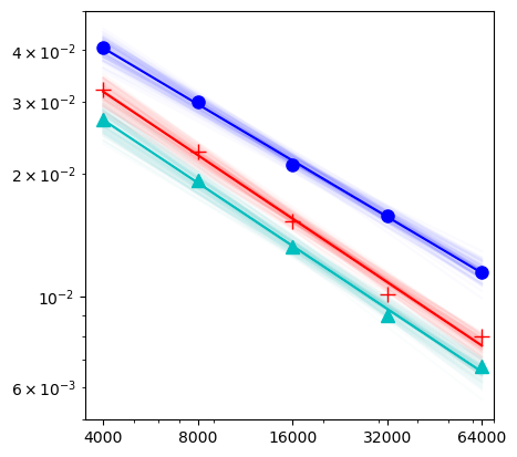
Figure 1: Comparisons of three approaches on a log-log plot. $x$-axis: $n$. $y$-axis: mean squared error. Red crosses: pseudo-labeling. Cyan triangles: the oracle method. Blue circles: the naïve method.

For every $n\in\{4000,8000,16000,32000,64000\}$, we run the experiment 100 times independently. Figure 1 shows the performances of three model selection approaches: pseudo-labeling (red crosses), the oracle method (cyan triangles) and the naïve method (blue circles). The $x$- and $y$-coordinates of each point are the sample size $n$ and the average of estimated excess risks over 100 independent runs, respectively. Since the points of each method are lined up on the log-log scale, the excess risk decays like $O(n^{-\alpha})$ for some $\alpha>0$. Linear regression yields the solid lines in Figure 1 and estimates the exponents $\alpha_{\mathrm{PL}}$ (pseudo-labeling), $\alpha_{\mathrm{oracle}}$ and $\alpha_{\text{na\"{i}ve}}$ as $0.516$, $0.511$ and $0.457$, respectively. We use cluster bootstrap (Cameron et al., 2008) to quantify the uncertainties, by resampling the $100$ data points corresponding to each $n$ for $10000$ times, independently of each other. The $95\%$ confidence intervals on $\alpha_{\mathrm{PL}}-\alpha_{\text{oracle}}$ and $\alpha_{\mathrm{PL}}-\alpha_{\text{na\"{i}ve}}$ are $[-0.024,0.031]$ and $[0.024,0.094]$, respectively. Our proposed method does not differ significantly from the oracle one in terms of the error exponent. It is significantly better than the naïve method. Indeed, the source data does not have a good coverage of the test cases. In addition, we also plot the linear fits of 100 bootstrap replicates to illustrate the stability, resulting in the thin shaded areas around the solid lines in Figure 1.

6 Proofs of Theorems 4.1 and 5.1

We now prove our main results: the excess risk bounds (Theorem 4.1) and the oracle inequality for model selection (Theorem 5.1). We will first conduct a fixed-design analysis in Section 6.1 by treating all the covariates and the data split as deterministic. After that, we will take the random designs into consideration and derive the final results in Section 6.2.

6.1 Fixed designs and the in-sample risk

To begin with, we tease out the impact of random errors $\{\varepsilon_{i}\}_{i=1}^{n}$ on our estimator $\widehat{f}$ by conditioning on the covariates $\{\bm{x}_{i}\}_{i=1}^{n}$, $\{\bm{x}_{0i}\}_{i=1}^{n_{0}}$ and the split $\mathcal{D}_{1}\cup\mathcal{D}_{2}$. As a result, we will study the in-sample risk $\mathcal{R}_{\mathrm{in}}$ defined in (5.2) and provide excess risk bounds as well as oracle inequalities.

To facilitate the analysis, we introduce some notation. When $\mathcal{X}=\mathbb{R}^{d}$ for some $d<\infty$ and $K(\bm{z},\bm{w})=\bm{z}^{\top}\bm{w}$, $\phi$ is the identity mapping. We can construct design matrices $\bm{X}=(\bm{x}_{1},\cdots,\bm{x}_{n})^{\top}\in\mathbb{R}^{n\times d}$, $\bm{X}_{0}=(\bm{x}_{01},\cdots,\bm{x}_{0n_{0}})^{\top}\in\mathbb{R}^{n_{0}\times d}$ and the response vector $\bm{y}=(y_{1},\cdots,y_{n})^{\top}\in\mathbb{R}^{n}$. Define the index set ${\mathcal{T}}=\{i\in[n]:~{}(\bm{x}_{i},y_{i})\in\mathcal{D}_{1}\}$ of the data for training candidate models. In addition, let $n_{1}=|{\mathcal{T}}|$ and $n_{2}=n-n_{1}$. Denote by $\bm{X}_{1}\in\mathbb{R}^{|{\mathcal{T}}|\times d}$ and $\bm{X}_{2}\in\mathbb{R}^{(n-|{\mathcal{T}}|)\times d}$ the sub-matrices of $\bm{X}$ by selecting rows whose indices belong to ${\mathcal{T}}$ and $[n]\backslash{\mathcal{T}}$, respectively. Similarly, denote by $\bm{y}_{1}\in\mathbb{R}^{|{\mathcal{T}}|}$ and $\bm{y}_{2}\in\mathbb{R}^{n-|{\mathcal{T}}|}$ the sub-vectors of $\bm{y}$ induced by those index sets.

The design matrices can be generalized to operators when $\mathcal{X}$ and $K$ are general. In that case, $\bm{X}$ and $\bm{X}_{0}$ are bounded linear operators defined through

$$\bm{X}:~{}\mathbb{H}\to\mathbb{R}^{n},~{}~{}\bm{\theta}\mapsto(\langle\phi(\bm{x}_{1}),\bm{\theta}\rangle,~{}\cdots,~{}\langle\phi(\bm{x}_{n}),\bm{\theta}\rangle)^{\top},$$

$$\bm{X}_{0}:~{}\mathbb{H}\to\mathbb{R}^{n_{0}},~{}~{}\bm{\theta}\mapsto(\langle\phi(\bm{x}_{01}),\bm{\theta}\rangle,~{}\cdots,~{}\langle\phi(\bm{x}_{0n_{0}}),\bm{\theta}\rangle)^{\top}.$$

We can define $\bm{X}_{1}$ and $\bm{X}_{2}$ similarly. With slight abuse of notation, we use $\bm{X}^{\top}$ to refer to the adjoint of $\bm{X}$, i.e. $\bm{X}^{\top}:~{}\mathbb{R}^{n}\to\mathbb{H}$, $\bm{u}\mapsto\sum_{i=1}^{n}u_{i}\phi(\bm{x}_{i})$. Similarly, we can define $\bm{X}_{0}^{\top}$, $\bm{X}_{1}^{\top}$ and $\bm{X}_{2}^{\top}$. Let $\widehat{\bm{\Sigma}}_{0}=\frac{1}{n_{0}}\sum_{i=1}^{n_{0}}\phi(\bm{x}_{0i})\otimes\phi(\bm{x}_{0i})$, $\widehat{\bm{\Sigma}}_{1}=\frac{1}{n_{1}}\sum_{i\in{\mathcal{T}}}\phi(\bm{x}_{i})\otimes\phi(\bm{x}_{i})$ and $\widehat{\bm{\Sigma}}_{2}=\frac{1}{n_{2}}\sum_{i\in[n]\backslash{\mathcal{T}}}\phi(\bm{x}_{i})\otimes\phi(\bm{x}_{i})$. We have $\widehat{\bm{\Sigma}}_{j}=n_{j}^{-1}\bm{X}_{j}^{\top}\bm{X}_{j}$ for all $j\in\{0,1,2\}$. Moreover, $\widehat{f}_{\lambda}(\cdot)=\langle\phi(\cdot),\widehat{\bm{\theta}}_{\lambda}\rangle$ holds for $\widehat{\bm{\theta}}_{\lambda}=(\widehat{\bm{\Sigma}}_{1}+\lambda\bm{I})^{-1}(n_{1}^{-1}\bm{X}_{1}^{\top}\bm{y}_{1})$, and $\widetilde{f}(\cdot)=\langle\phi(\cdot),\widetilde{\bm{\theta}}\rangle$ holds for $\widetilde{\bm{\theta}}=(\widehat{\bm{\Sigma}}_{2}+\widetilde{\lambda}\bm{I})^{-1}(n_{2}^{-1}\bm{X}_{2}^{\top}\bm{y}_{2})$.

Below we present a lemma on kernel ridge regression that plays a major role throughout the analysis. See Appendix A.1 for its proof.

Lemma 6.1 (Fixed-design KRR).

Let Assumptions 2.2 and 4.1 hold, with the exception that $\{\bm{x}_{i}\}_{i=1}^{n}$ and $\{\bm{x}_{0i}\}_{i=1}^{n_{0}}$ are deterministic. Let the partition $\mathcal{D}_{1}\cup\mathcal{D}_{2}$ be fixed. Choose any $\lambda>0$ and define $\bar{\bm{\theta}}_{\lambda}=\mathbb{E}\widehat{\bm{\theta}}_{\lambda}$.

1. There exist universal constants $C_{1}$ and $C_{2}$ such that

   $$\|\bar{\bm{\theta}}_{\lambda}-\bm{\theta}^{\star}\|_{\mathbb{H}}\leq\|\bm{\theta}^{\star}\|_{\mathbb{H}},$$

   $$\|\widehat{\bm{\theta}}_{\lambda}-\bar{\bm{\theta}}_{\lambda}\|_{\psi_{2}}\leq\frac{C_{1}\sigma}{\sqrt{n_{1}\lambda}},$$

   $$\|n_{0}^{-1/2}\bm{X}_{0}(\bar{\bm{\theta}}_{\lambda}-\bm{\theta}^{\star})\|_{2}\leq\sqrt{\lambda\|(\widehat{\bm{\Sigma}}_{1}+\lambda\bm{I})^{-1/2}\widehat{\bm{\Sigma}}_{0}(\widehat{\bm{\Sigma}}_{1}+\lambda\bm{I})^{-1/2}\|}\cdot\|\bm{\theta}^{\star}\|_{\mathbb{H}},$$

   $$\|n_{0}^{-1/2}\bm{X}_{0}(\widehat{\bm{\theta}}_{\lambda}-\bar{\bm{\theta}}_{\lambda})\|_{\psi_{2}}\leq C_{1}\sigma\sqrt{\frac{\|(\widehat{\bm{\Sigma}}_{1}+\lambda\bm{I})^{-1/2}\widehat{\bm{\Sigma}}_{0}(\widehat{\bm{\Sigma}}_{1}+\lambda\bm{I})^{-1/2}\|}{n_{1}}},$$

   $$\mathbb{P}\bigg{(}\|\widehat{\bm{\theta}}_{\lambda}-\bm{\theta}^{\star}\|_{\mathbb{H}}\leq\|\bm{\theta}^{\star}\|_{\mathbb{H}}+\sqrt{\frac{C_{2}\sigma^{2}\log(1/\delta)}{n_{1}\lambda}\mathop{\mathrm{Tr}}[(\widehat{\bm{\Sigma}}_{1}+\lambda\bm{I})^{-1}\widehat{\bm{\Sigma}}_{1}]}\bigg{)}\geq 1-\delta,~{}~{}\forall\delta\in(0,1/e].$$

2. Choose any positive semi-definite trace class operator $\bm{Q}:~{}\mathbb{H}\to\mathbb{H}$ and define $\widehat{\bm{S}}_{\lambda}=(\widehat{\bm{\Sigma}}_{1}+\lambda\bm{I})^{-1/2}\bm{Q}(\widehat{\bm{\Sigma}}_{1}+\lambda\bm{I})^{-1/2}$. We have

   $$\mathbb{P}\bigg{(}\|\widehat{\bm{\theta}}_{\lambda}-\bm{\theta}^{\star}\|_{\bm{Q}}^{2}\leq 2\lambda\|\widehat{\bm{S}}_{\lambda}\|\cdot\|\bm{\theta}^{\star}\|_{\mathbb{H}}^{2}+\frac{2C_{2}\sigma^{2}\mathop{\mathrm{Tr}}(\widehat{\bm{S}}_{\lambda})}{n_{1}}\log(1/\delta)\bigg{)}\geq 1-\delta,~{}~{}\forall\delta\in(0,1/e].$$

With the help of Lemma 6.1, we can easily control the excess in-sample risks of the candidate models using some function $\widehat{\mathcal{E}}(\lambda,\delta)$ that is an empirical version of $\mathcal{E}(\lambda,\delta)$ in Theorem 4.1. The quantity $\delta$ is the exceptional probability. The optimal candidate in $\{\widehat{f}_{\lambda}\}_{\lambda\in\Lambda}$ is near-optimal over an enlarged set $\{\widehat{f}_{\lambda}\}_{\lambda_{\min}\leq\lambda\leq\lambda_{\max}}$ up to a multiplicative factor, as long as $\lambda_{j+1}/\lambda_{j}$ is bounded. We can also derive from Lemma 6.1 and Theorem 5.2 an oracle inequality of the form (5.4) showing that the excess in-sample risk $\mathcal{R}_{\mathrm{in}}(\widehat{f})-\mathcal{R}_{\mathrm{in}}(f^{\star})$ of our selected model is a small multiple of $\min_{\lambda\in\Lambda}[\mathcal{R}_{\mathrm{in}}(\widehat{f}_{\lambda})-\mathcal{R}_{\mathrm{in}}(f^{\star})]$ plus some overhead $\widehat{\xi}(\widetilde{\lambda},\delta)$. The latter reflects the error of the imputation model $\widetilde{f}$, and it is an empirical version of $\xi(\widetilde{\lambda},\delta)$. The results are summarized in Theorem 6.1 below.

Theorem 6.1 (In-sample risks).

Let Assumptions 2.2 and 4.1 hold. Suppose that $\Lambda=\{\lambda_{1},\cdots,\lambda_{m}\}$, $m\geq 2$, and $0<\lambda_{j}<\lambda_{j+1}\leq\beta\lambda_{j}$ holds for all $j\in[m-1]$ and some $\beta\geq 1$. For any $\lambda>0$ and $\delta\in(0,1/e]$, define

$$\widehat{\bm{S}}_{j,\lambda}=(\widehat{\bm{\Sigma}}_{j}+\lambda\bm{I})^{-1/2}\widehat{\bm{\Sigma}}_{0}(\widehat{\bm{\Sigma}}_{j}+\lambda\bm{I})^{-1/2},\qquad j\in\{1,2\},$$

$$\widehat{\mathcal{E}}(\lambda,\delta)=\lambda\|\widehat{\bm{S}}_{1,\lambda}\|\cdot\|\bm{\theta}^{\star}\|_{\mathbb{H}}^{2}+\frac{\sigma^{2}\mathop{\mathrm{Tr}}(\widehat{\bm{S}}_{1,\lambda})\log(m/\delta)}{n_{1}},$$

$$\widehat{\xi}(\lambda,\delta)=\bigg{(}\lambda\|\bm{\theta}^{\star}\|_{\mathbb{H}}^{2}+\frac{\sigma^{2}\log(m/\delta)}{n_{2}}\bigg{)}\|\widehat{\bm{S}}_{2,\widetilde{\lambda}}\|.$$

There exist universal constants $C_{1}$ and $C_{2}$ such that with probability at least $1-\delta$, we have

$$\min_{\lambda\in\Lambda}\mathcal{R}_{\mathrm{in}}(\widehat{f}_{\lambda})-\mathcal{R}_{\mathrm{in}}(f^{\star})\leq C_{1}\beta\min_{\lambda_{1}\leq\lambda\leq\lambda_{m}}\widehat{\mathcal{E}}(\lambda,\delta),$$

$$\mathcal{R}_{\mathrm{in}}(\widehat{f})-\mathcal{R}_{\mathrm{in}}(f^{\star})\leq\inf_{\gamma>0}\bigg{\{}(1+\gamma)\min_{\lambda\in\Lambda}[\mathcal{R}_{\mathrm{in}}(\widehat{f}_{\lambda})-\mathcal{R}_{\mathrm{in}}(f^{\star})]+C_{2}(1+\gamma^{-1})\widehat{\xi}(\widetilde{\lambda},\delta)\bigg{\}}.$$

When that event happens,

$$\mathcal{R}_{\mathrm{in}}(\widehat{f})-\mathcal{R}_{\mathrm{in}}(f^{\star})\leq\inf_{\gamma>0}\bigg{\{}(1+\gamma)C_{1}\beta\min_{\lambda_{1}\leq\lambda\leq\lambda_{m}}\widehat{\mathcal{E}}(\lambda,\delta)+C_{2}(1+\gamma^{-1})\widehat{\xi}(\widetilde{\lambda},\delta)\bigg{\}}.$$

Proof of Theorem 6.1.

First of all, it is easily seen from the decomposition (5.3) that

$$\mathcal{R}_{\mathrm{in}}(\widehat{f}_{\lambda})-\mathcal{R}_{\mathrm{in}}(f^{\star})=\|\widehat{\bm{\theta}}_{\lambda}-\bm{\theta}^{\star}\|_{\widehat{\bm{\Sigma}}_{0}}^{2}.$$

Part 2 of Lemma 6.1 (with $\bm{Q}=\widehat{\bm{\Sigma}}_{0}$) and union bounds imply the existence of a universal constant $C_{1}$ such that

$$\mathbb{P}\bigg{(}\mathcal{R}_{\mathrm{in}}(\widehat{f}_{\lambda})-\mathcal{R}_{\mathrm{in}}(f^{\star})\leq C_{1}\widehat{\mathcal{E}}(\lambda,\delta),~{}~{}\forall\lambda\in\Lambda\bigg{)}\geq 1-\delta/2,\qquad\forall\delta\in(0,1/e].$$

Denote by $\mathcal{A}$ the above event. When $\mathcal{A}$ happens, we have

$$\min_{\lambda\in\Lambda}\mathcal{R}_{\mathrm{in}}(\widehat{f}_{\lambda})-\mathcal{R}_{\mathrm{in}}(f^{\star})\leq C_{1}\min_{\lambda\in\Lambda}\widehat{\mathcal{E}}(\lambda,\delta).$$

Next, we bridge the discrete index set $\Lambda$ and the interval $[\lambda_{1},\lambda_{m}]$. For any $\lambda>0$, $t\geq 1$ and $j\in\{1,2\}$, we have $(\widehat{\bm{\Sigma}}_{j}+t\lambda\bm{I})^{-1}\succeq t^{-1}(\widehat{\bm{\Sigma}}_{j}+\lambda\bm{I})^{-1}$. Then, $\mathop{\mathrm{Tr}}(\widehat{\bm{S}}_{j,t\lambda})\geq t^{-1}\mathop{\mathrm{Tr}}(\widehat{\bm{S}}_{j,\lambda})$, $\|\widehat{\bm{S}}_{j,t\lambda}\|\geq t^{-1}\|\widehat{\bm{S}}_{j,\lambda}\|$ and $t\lambda\|\widehat{\bm{S}}_{j,t\lambda}\|\geq\lambda\|\widehat{\bm{S}}_{j,\lambda}\|$. As a result, $\widehat{\mathcal{E}}(t\lambda,\delta)\geq t^{-1}\widehat{\mathcal{E}}(\lambda,\delta)$. It follows from $0<\lambda_{j}<\lambda_{j+1}\leq\beta\lambda_{j}$ that for any $\lambda\in[\lambda_{j},\lambda_{j+1}]$,

$$\widehat{\mathcal{E}}(\lambda,\delta)\geq\frac{\lambda_{j}}{\lambda}\widehat{\mathcal{E}}(\lambda_{j},\delta)\geq\beta^{-1}\widehat{\mathcal{E}}(\lambda_{j},\delta).$$

Therefore, $\min_{\lambda_{1}\leq\lambda\leq\lambda_{m}}\widehat{\mathcal{E}}(\lambda,\delta)\geq\beta^{-1}\min_{\lambda\in\Lambda}\widehat{\mathcal{E}}(\lambda,\delta)$. We have

$$\mathbb{P}\bigg{(}\min_{\lambda\in\Lambda}\mathcal{R}_{\mathrm{in}}(\widehat{f}_{\lambda})-\mathcal{R}_{\mathrm{in}}(f^{\star})\leq C_{1}\beta\min_{\lambda_{1}\leq\lambda\leq\lambda_{m}}\widehat{\mathcal{E}}(\lambda,\delta)\bigg{)}\geq\mathbb{P}(\mathcal{A})\geq 1-\delta/2.$$

We now prove an oracle inequality for $\widehat{f}$. Define $\bm{y}^{\star}=\bm{X}_{0}\bm{\theta}^{\star}=(f^{\star}(\bm{x}_{01}),~{}\cdots,f^{\star}(\bm{x}_{0n_{0}}))^{\top}$, $\widetilde{\bm{y}}=\bm{X}_{0}\widetilde{\bm{\theta}}=(\widetilde{f}(\bm{x}_{01}),~{}\cdots,\widetilde{f}(\bm{x}_{0n_{0}}))^{\top}$ and $\bar{\bm{\theta}}=\mathbb{E}(\widetilde{\bm{\theta}}|\bm{X}_{2})$. Applying Part 1 in Lemma 6.1 to $\widetilde{\bm{\theta}}$ shows that

$$n_{0}^{-1/2}\|\mathbb{E}\widetilde{\bm{y}}-\bm{y}^{\star}\|_{2}=\|n_{0}^{-1/2}\bm{X}_{0}(\bar{\bm{\theta}}-\bm{\theta}^{\star})\|_{2}\leq\sqrt{\widetilde{\lambda}\|\widehat{\bm{S}}_{2,\widetilde{\lambda}}\|}\cdot\|\bm{\theta}^{\star}\|_{\mathbb{H}},$$

$$n_{0}^{-1/2}\|\widetilde{\bm{y}}-\mathbb{E}\widetilde{\bm{y}}\|_{\psi_{2}}=\|n_{0}^{-1/2}\bm{X}_{0}(\widetilde{\bm{\theta}}-\bar{\bm{\theta}})\|_{\psi_{2}}\lesssim\frac{\sigma}{\sqrt{n_{2}}}\sqrt{\|\widehat{\bm{S}}_{2,\widetilde{\lambda}}\|},$$

where $\lesssim$ only hides a universal constant factor. Theorem 5.2 immediately yields the existence of a universal constant $C_{2}$ such that

$$\mathbb{P}\bigg{(}\mathcal{R}_{\mathrm{in}}(\widehat{f})-\mathcal{R}_{\mathrm{in}}(f^{\star})\leq\inf_{\gamma>0}\bigg{\{} (1+\gamma)\min_{\lambda\in\Lambda}[\mathcal{R}_{\mathrm{in}}(\widehat{f}_{\lambda})-\mathcal{R}_{\mathrm{in}}(f^{\star})]$$

$$+C_{2}(1+\gamma^{-1})\widehat{\xi}(\widetilde{\lambda},\delta)\bigg{\}}\bigg{)}\geq 1-\delta/2.$$

Finally, the proof is completed by combining the above estimates by union bounds. ∎

6.2 Random designs and the out-of-sample risk

6.2.1 Two lemmas

To analyze the estimator $\widehat{f}$ in the random design setting, we need to $\mathrm{(i)}$ bound the deviations of the empirical second-moment operators $\{\widehat{\bm{\Sigma}}_{j}\}_{j=0}^{2}$ from their population versions, and $\mathrm{(ii)}$ relate the excess in-sample risk to the out-of-sample version. The following two lemmas are devoted to them. Their proofs are deferred to Appendices A.2 and A.3.

Lemma 6.2 (Concentration of second-moment operators).

Choose any $\delta\in(0,1/5]$ and let Assumption 2.2 hold.

1. Under Assumption 4.2, there exists a universal constant $C$ such that the following inequalities hold simultaneously with probability at least $1-\delta$:

   $$\widehat{\bm{\Sigma}}_{0}\preceq\frac{3}{2}\bigg{(}\bm{\Sigma}_{0}+\frac{CM^{2}\log(3n_{0}/\delta)}{3n_{0}}\bm{I}\bigg{)},$$

   $$\widehat{\bm{\Sigma}}_{1}+\lambda\bm{I}\succeq\frac{1}{2}(\bm{\Sigma}+\lambda\bm{I}),\qquad\forall\lambda\geq\frac{CM^{2}\log(3n/\delta)}{(1-\rho)n},$$

   $$\widehat{\bm{\Sigma}}_{2}+\widetilde{\lambda}\bm{I}\succeq\frac{1}{2}(\bm{\Sigma}+\widetilde{\lambda}\bm{I}),\qquad\forall\widetilde{\lambda}\geq\frac{CM^{2}\log(3n/\delta)}{\rho n}.$$

   On the above event, for all $\lambda\geq\frac{CM^{2}\log(3n/\delta)}{(1-\rho)n}$ and $\widetilde{\lambda}\geq\frac{CM^{2}\log(3n/\delta)}{\rho n}$ we have

   $$\mathop{\mathrm{Tr}}[(\widehat{\bm{\Sigma}}_{1}+\lambda\bm{I})^{-1/2}\bm{\Sigma}_{0}(\widehat{\bm{\Sigma}}_{1}+\lambda\bm{I})^{-1/2}]\leq 2\mathop{\mathrm{Tr}}[(\bm{\Sigma}+\lambda\bm{I})^{-1/2}\bm{\Sigma}_{0}(\bm{\Sigma}+\lambda\bm{I})^{-1/2}],$$

   $$\|(\widehat{\bm{\Sigma}}_{1}+\lambda\bm{I})^{-1/2}\bm{\Sigma}_{0}(\widehat{\bm{\Sigma}}_{1}+\lambda\bm{I})^{-1/2}\|\leq 2\|(\bm{\Sigma}+\lambda\bm{I})^{-1/2}\bm{\Sigma}_{0}(\bm{\Sigma}+\lambda\bm{I})^{-1/2}\|,$$

   $$\|(\widehat{\bm{\Sigma}}_{2}+\widetilde{\lambda}\bm{I})^{-1/2}\widehat{\bm{\Sigma}}_{0}(\widehat{\bm{\Sigma}}_{2}+\widetilde{\lambda}\bm{I})^{-1/2}\|\leq 3\|(\bm{\Sigma}+\widetilde{\lambda}\bm{I})^{-1/2}\bm{\Sigma}_{0}(\bm{\Sigma}+\widetilde{\lambda}\bm{I})^{-1/2}\|$$

   $$\qquad\qquad\qquad\qquad\qquad\qquad\qquad\qquad+\frac{n}{n_{0}}\max\bigg{\{}1,~{}\frac{\log n_{0}}{\log n}\bigg{\}}.$$

2. Under Assumption 4.3, there exists a constant $C\geq 1$ determined by $\kappa$ such that the following inequalities hold simultaneously with probability at least $1-\delta$:

   $$\widehat{\bm{\Sigma}}_{0}\preceq\frac{3}{2}\bigg{(}\bm{\Sigma}_{0}+\frac{C\mathop{\mathrm{Tr}}(\bm{\Sigma}_{0})\log(3/\delta)}{3n_{0}}\bm{I}\bigg{)},$$

   $$\widehat{\bm{\Sigma}}_{1}+\lambda\bm{I}\succeq\frac{1}{2}(\bm{\Sigma}+\lambda\bm{I}),\qquad\forall\lambda\geq\frac{C\mathop{\mathrm{Tr}}(\bm{\Sigma})\log(3/\delta)}{(1-\rho)n},$$

   $$\widehat{\bm{\Sigma}}_{2}+\widetilde{\lambda}\bm{I}\succeq\frac{1}{2}(\bm{\Sigma}+\widetilde{\lambda}\bm{I}),\qquad\forall\widetilde{\lambda}\geq\frac{C\mathop{\mathrm{Tr}}(\bm{\Sigma})\log(3/\delta)}{\rho n}.$$

   On the above event, for all $\lambda\geq\frac{C\mathop{\mathrm{Tr}}(\bm{\Sigma})\log(3/\delta)}{(1-\rho)n}$ and $\widetilde{\lambda}\geq\frac{C\mathop{\mathrm{Tr}}(\bm{\Sigma})\log(3/\delta)}{\rho n}$ we have same estimates on $\mathop{\mathrm{Tr}}[(\widehat{\bm{\Sigma}}_{1}+\lambda\bm{I})^{-1/2}\bm{\Sigma}_{0}(\widehat{\bm{\Sigma}}_{1}+\lambda\bm{I})^{-1/2}]$ and $\|(\widehat{\bm{\Sigma}}_{1}+\lambda\bm{I})^{-1/2}\bm{\Sigma}_{0}(\widehat{\bm{\Sigma}}_{1}+\lambda\bm{I})^{-1/2}\|$ as in Part 1, and

   $$\|(\widehat{\bm{\Sigma}}_{2}+\widetilde{\lambda}\bm{I})^{-1/2}\widehat{\bm{\Sigma}}_{0}(\widehat{\bm{\Sigma}}_{2}+\widetilde{\lambda}\bm{I})^{-1/2}\|\leq 3\|(\bm{\Sigma}+\widetilde{\lambda}\bm{I})^{-1/2}\bm{\Sigma}_{0}(\bm{\Sigma}+\widetilde{\lambda}\bm{I})^{-1/2}\|+\frac{n}{n_{0}}\cdot\frac{\mathop{\mathrm{Tr}}(\bm{\Sigma}_{0})}{\mathop{\mathrm{Tr}}(\bm{\Sigma})}.$$

Lemma 6.3 (In-sample and out-of-sample risks).

Let Assumptions 2.2 and 4.1 hold. Choose any $\delta\in(1,1/e]$ and $\gamma\in(0,3/4]$.

1. Suppose that Assumption 4.2 holds and $\min_{\lambda\in\Lambda}\lambda\geq\frac{8M^{2}\log[(n+n_{0})|\Lambda|/\delta]}{(1-\rho)n}$. Define

   $$\zeta(\delta)=\frac{(\|\bm{\theta}^{\star}\|_{\mathbb{H}}M+\sigma)^{2}\log(|\Lambda|/\delta)}{n_{0}}.$$

   There exists a universal constant $C_{0}$ such that with probability at least $1-\delta$, the following inequality holds simultaneously for all $\lambda\in|\Lambda|$:

   $$(1-\gamma)[\mathcal{R}(\widehat{f}_{\lambda})-\mathcal{R}(f^{\star})]-\frac{C_{0}}{\gamma}\zeta(\delta) \leq\mathcal{R}_{\mathrm{in}}(\widehat{f}_{\lambda})-\mathcal{R}_{\mathrm{in}}(f^{\star})$$

   $$\leq(1+\gamma)[\mathcal{R}(\widehat{f}_{\lambda})-\mathcal{R}(f^{\star})]+\frac{C_{0}}{\gamma}\zeta(\delta).$$

2. Suppose that Assumption 4.3 holds. There exists a universal constant $C>0$ such that when $n_{0}\geq(C\kappa/\gamma)^{2}\log(|\Lambda|/\delta)$, the following inequality holds with probability at least $1-\delta$:

   $$(1-\gamma)[\mathcal{R}(\widehat{f}_{\lambda})-\mathcal{R}(f^{\star})]\leq\mathcal{R}_{\mathrm{in}}(\widehat{f}_{\lambda})-\mathcal{R}_{\mathrm{in}}(f^{\star})\leq(1+\gamma)[\mathcal{R}(\widehat{f}_{\lambda})-\mathcal{R}(f^{\star})].$$

Equipped with those technical tools, we are now ready to tackle Theorems 5.1 and 4.1.

6.2.2 Proof of Theorem 5.1

Under Assumption 4.2 or 4.3, Lemma 6.2 implies that when $C$ is large enough,

$$\mathbb{P}\bigg{(}\widehat{\xi}(\widetilde{\lambda},\delta)\leq 3\xi(\widetilde{\lambda},\delta)\bigg{)}\geq 1-\delta/3.$$

Combining the above with Theorem 6.1, we see that when $\gamma\in(0,3/4]$ and $C$ is large enough, there exists a large constant $C_{1}$ such that with probability at least $1-\delta/2$,

$$\mathcal{R}_{\mathrm{in}}(\widehat{f})-\mathcal{R}_{\mathrm{in}}(f^{\star})\leq(1+\gamma)\min_{\lambda\in\Lambda}[\mathcal{R}_{\mathrm{in}}(\widehat{f}_{\lambda})-\mathcal{R}_{\mathrm{in}}(f^{\star})]+\frac{C_{1}}{\gamma}\xi(\widetilde{\lambda},\delta).$$

Denote by $\mathcal{A}$ the above event.

On the other hand, Lemma 6.3 implies that when $C$ is large enough, there exists a large constant $C_{2}$ such that with probability at least $1-\delta/2$, the following bound holds simultaneously for all $\lambda\in\Lambda$:

$$(1-\gamma)[\mathcal{R}(\widehat{f}_{\lambda})-\mathcal{R}(f^{\star})]-\frac{C_{2}}{\gamma}\zeta(\delta) \leq\mathcal{R}_{\mathrm{in}}(\widehat{f}_{\lambda})-\mathcal{R}_{\mathrm{in}}(f^{\star})$$

$$\leq(1+\gamma)[\mathcal{R}(\widehat{f}_{\lambda})-\mathcal{R}(f^{\star})]+\frac{C_{2}}{\gamma}\zeta(\delta).$$

Denote by $\mathcal{B}$ the above event.

• Under Assumption 4.2, we have $\zeta(\delta)=\frac{(\|\bm{\theta}^{\star}\|_{\mathbb{H}}M+\sigma)^{2}\log(|\Lambda|/\delta)}{n_{0}}$. We use the assumptions $\widetilde{\lambda}\gtrsim\frac{M^{2}\log(n/\delta)}{\rho n}$ and $|\Lambda|\leq n^{c}$ to derive that

  $$\zeta(\delta) \lesssim\frac{(\|\bm{\theta}^{\star}\|_{\mathbb{H}}^{2}M^{2}+\sigma^{2})\log(|\Lambda|/\delta)}{n_{0}}\lesssim\frac{(\|\bm{\theta}^{\star}\|_{\mathbb{H}}^{2}\frac{\widetilde{\lambda}\rho n}{\log(n/\delta)}+\sigma^{2})\log(|\Lambda|/\delta)}{n_{0}}$$

  $$=\bigg{(}\frac{\log(|\Lambda|/\delta)}{\log(n/\delta)}\cdot\widetilde{\lambda}\|\bm{\theta}^{\star}\|_{\mathbb{H}}^{2}+\frac{\sigma^{2}\log(|\Lambda|/\delta)}{\rho n}\bigg{)}\cdot\frac{\rho n}{n_{0}}$$

  $$\leq\bigg{(}\widetilde{\lambda}\|\bm{\theta}^{\star}\|_{\mathbb{H}}^{2}+\frac{\sigma^{2}\log(|\Lambda|/\delta)}{\rho n}\bigg{)}\cdot\frac{n}{n_{0}}\leq\xi(\widetilde{\lambda},\delta).$$

• Under Assumption 4.3, we have $\zeta(\delta)=0\leq\xi(\widetilde{\lambda},\delta)$.

Based on the above, we always have $\zeta(\delta)\lesssim\xi(\widetilde{\lambda},\delta)$. When the event $\mathcal{B}$ happens, we have

$$\mathcal{R}(\widehat{f})-\mathcal{R}(f^{\star})\leq\frac{1}{1-\gamma}\bigg{(}[\mathcal{R}_{\mathrm{in}}(\widehat{f})-\mathcal{R}_{\mathrm{in}}(f^{\star})]+\frac{C_{2}}{\gamma}\xi(\widetilde{\lambda},\delta)\bigg{)},$$

$$\min_{\lambda\in\Lambda}[\mathcal{R}_{\mathrm{in}}(\widehat{f}_{\lambda})-\mathcal{R}_{\mathrm{in}}(f^{\star})]\leq(1+\gamma)\min_{\lambda\in\Lambda}[\mathcal{R}(\widehat{f}_{\lambda})-\mathcal{R}(f^{\star})]+\frac{C_{2}}{\gamma}\xi(\widetilde{\lambda},\delta).$$

When the event $\mathcal{A}\cap\mathcal{B}$ happens (which has probability at least $1-\delta$), we have

$$\mathcal{R}(\widehat{f})-\mathcal{R}(f^{\star})\leq\frac{1}{1-\gamma}\bigg{(}[\mathcal{R}_{\mathrm{in}}(\widehat{f})-\mathcal{R}_{\mathrm{in}}(f^{\star})]+\frac{C_{2}}{\gamma}\xi(\widetilde{\lambda},\delta)\bigg{)}$$

$$\leq\frac{1}{1-\gamma}\bigg{[}\bigg{(}(1+\gamma)\min_{\lambda\in\Lambda}[\mathcal{R}_{\mathrm{in}}(\widehat{f}_{\lambda})-\mathcal{R}_{\mathrm{in}}(f^{\star})]+\frac{C_{1}}{\gamma}\xi(\widetilde{\lambda},\delta)\bigg{)}+\frac{C_{2}}{\gamma}\xi(\widetilde{\lambda},\delta)\bigg{]}$$

$$=\frac{1+\gamma}{1-\gamma}\min_{\lambda\in\Lambda}[\mathcal{R}_{\mathrm{in}}(\widehat{f}_{\lambda})-\mathcal{R}_{\mathrm{in}}(f^{\star})]+\frac{(C_{1}+C_{2})\xi(\widetilde{\lambda},\delta)}{\gamma(1-\gamma)}$$

$$\leq\frac{1+\gamma}{1-\gamma}\bigg{(}(1+\gamma)\min_{\lambda\in\Lambda}[\mathcal{R}(\widehat{f}_{\lambda})-\mathcal{R}(f^{\star})]+\frac{C_{2}}{\gamma}\xi(\widetilde{\lambda},\delta)\bigg{)}+\frac{(C_{1}+C_{2})\xi(\widetilde{\lambda},\delta)}{\gamma(1-\gamma)}$$

$$=\frac{(1+\gamma)^{2}}{1-\gamma}\min_{\lambda\in\Lambda}[\mathcal{R}(\widehat{f}_{\lambda})-\mathcal{R}(f^{\star})]+\frac{[C_{1}+(2+\gamma)C_{2}]\xi(\widetilde{\lambda},\delta)}{\gamma(1-\gamma)}.$$

By $\gamma\in(0,3/4]$, we have $2+\gamma\leq 3$, $\frac{1}{1-\gamma}\leq 4$ and

$$\frac{(1+\gamma)^{2}}{1-\gamma}=\frac{1+2\gamma+\gamma^{2}}{1-\gamma}=1+\frac{3\gamma+\gamma^{2}}{1-\gamma}=1+\gamma\cdot\frac{3+\gamma}{1-\gamma}\leq 1+16\gamma.$$

Hence, there exists a constant $C_{3}$ such that

$$\mathbb{P}\bigg{(}\mathcal{R}(\widehat{f})-\mathcal{R}(f^{\star})\leq(1+16\gamma)\min_{\lambda\in\Lambda}[\mathcal{R}(\widehat{f}_{\lambda})-\mathcal{R}(f^{\star})]+\frac{C_{3}}{\gamma}\xi(\widetilde{\lambda},\delta)\bigg{)}\geq 1-\delta.$$

By redefining $\gamma$ and choosing a sufficiently large $C_{0}$, we get the desired result.

6.2.3 Proof of Theorem 4.1

Under Assumption 4.2 or 4.3, Lemma 6.2 implies that when $C$ is large enough,

$$\mathbb{P}\bigg{(}\|\widehat{\bm{S}}_{1,\lambda}\|\leq 2\|\bm{S}_{\lambda}\|\text{ and }\mathop{\mathrm{Tr}}(\widehat{\bm{S}}_{1,\lambda})\leq 2\mathop{\mathrm{Tr}}(\bm{S}_{\lambda})\bigg{)}\geq 1-\delta/2.$$

Then, the desired results follow from Theorem 6.1, Theorem 5.1 and union bounds.

7 Discussion

We developed a simple approach for kernel ridge regression under covariate shift. A key component is an imputation model that generates pseudo-labels for model selection. The final estimator is shown to adapt to the covariate shift in many common scenarios. We hope that our work can spur further research toward a systematic solution to covariate shift problems. Lots of open questions are worth studying. For instance, we need general measures of covariate shift and corresponding tools for handling them. When $\bm{\Sigma}_{0}\preceq B\bm{\Sigma}$ (a special case is $\frac{\mathrm{d}Q}{\mathrm{d}P}\leq B$), our approach achieves the minimax optimal error rate without knowing $B$. It would be interesting to consider other discrepancy measures such as divergences or Wasserstein metrics. Our two-stage approach with separate uses of source and target data may need modification. The candidate models may better be trained using some weighted loss based on the target data. Another direction is statistical learning over general function classes. The current paper only considered kernel ridge regression with well-specified model. Analytical expressions of the fitted models greatly facilitated our theoretical analysis. In future work, we would like to go beyond that and develop more versatile methods.

Appendix A Proofs of Lemmas 6.1, 6.2 and 6.3

A.1 Proof of Lemma 6.1

A.1.1 Part 1

Analysis of $\|\widehat{\bm{\theta}}_{\lambda}-\bm{\theta}^{\star}\|_{\psi_{2}}$ and $\|\widehat{\bm{\theta}}_{\lambda}-\bm{\theta}^{\star}\|_{\mathbb{H}}$. Define $\bm{\varepsilon}_{1}=\bm{y}_{1}-\bm{X}_{1}\bm{\theta}^{\star}$. Under Assumption 2.2,

$$\bar{\bm{\theta}}_{\lambda}=(\widehat{\bm{\Sigma}}_{1}+\lambda\bm{I})^{-1}(n_{1}^{-1}\bm{X}_{1}^{\top}\bm{y}_{1})=(\widehat{\bm{\Sigma}}_{1}+\lambda\bm{I})^{-1}\widehat{\bm{\Sigma}}_{1}\bm{\theta}^{\star},$$

$$\bar{\bm{\theta}}_{\lambda}-\bm{\theta}^{\star}=-\lambda(\widehat{\bm{\Sigma}}_{1}+\lambda\bm{I})^{-1}\bm{\theta}^{\star},$$ (A.1)

$$\widehat{\bm{\theta}}_{\lambda}-\bar{\bm{\theta}}_{\lambda}=(\widehat{\bm{\Sigma}}_{1}+\lambda\bm{I})^{-1}(n_{1}^{-1}\bm{X}_{1}^{\top}\bm{\varepsilon}_{1}).$$ (A.2)

On the one hand,

$$\|\bar{\bm{\theta}}_{\lambda}-\bm{\theta}^{\star}\|_{\mathbb{H}}=\lambda\|(\widehat{\bm{\Sigma}}_{1}+\lambda\bm{I})^{-1}\bm{\theta}^{\star}\|_{\mathbb{H}}\leq\|\bm{\theta}^{\star}\|_{\mathbb{H}}.$$ (A.3)

On the other hand, note that $(\widehat{\bm{\Sigma}}_{1}+\lambda\bm{I})^{-1}(n_{1}^{-2}\bm{X}_{1}^{\top}):~{}\mathbb{R}^{n}\to\mathbb{H}$ is a bounded linear operator whose adjoint is $(n_{1}^{-2}\bm{X}_{1})(\widehat{\bm{\Sigma}}_{1}+\lambda\bm{I})^{-1}$. Hence,

$$\|(\widehat{\bm{\Sigma}}_{1}+\lambda\bm{I})^{-1}(n_{1}^{-1}\bm{X}_{1}^{\top})\|^{2}=\|(\widehat{\bm{\Sigma}}_{1}+\lambda\bm{I})^{-1}(n_{1}^{-1}\bm{X}_{1}^{\top})(n_{1}^{-1}\bm{X}_{1})(\widehat{\bm{\Sigma}}_{1}+\lambda\bm{I})^{-1}\|$$

$$=n_{1}^{-1}\|(\widehat{\bm{\Sigma}}_{1}+\lambda\bm{I})^{-1}\widehat{\bm{\Sigma}}_{1}(\widehat{\bm{\Sigma}}_{1}+\lambda\bm{I})^{-1}\|\leq(n_{1}\lambda)^{-1}.$$

Assumption 4.1 implies the following fact with $C_{1}$ being a universal constant.

Fact A.1.

$\bm{\varepsilon}_{1}$ has sub-Gaussian norm bounded by $C_{1}\sigma$.

By Fact A.1,

$$\|\widehat{\bm{\theta}}_{\lambda}-\bar{\bm{\theta}}_{\lambda}\|_{\psi_{2}}=\|(\widehat{\bm{\Sigma}}_{1}+\lambda\bm{I})^{-1}(n_{1}^{-1}\bm{X}_{1}^{\top})\bm{\varepsilon}_{1}\|_{\psi_{2}}\leq\frac{\|\bm{\varepsilon}_{1}\|_{\psi_{2}}}{\sqrt{n_{1}\lambda}}\leq\frac{C_{1}\sigma}{\sqrt{n_{1}\lambda}}.$$

Next, we prove the tail bound on $\|\widehat{\bm{\theta}}_{\lambda}-\bm{\theta}^{\star}\|_{\mathbb{H}}$. The representation (A.2) yields

$$\|\widehat{\bm{\theta}}_{\lambda}-\bar{\bm{\theta}}_{\lambda}\|_{\mathbb{H}}^{2}=\frac{1}{n_{1}^{2}}\langle\bm{\varepsilon}_{1},\bm{X}_{1}(\widehat{\bm{\Sigma}}_{1}+\lambda\bm{I})^{-2}\bm{X}_{1}^{\top}\bm{\varepsilon}_{1}\rangle.$$

By Fact A.1 and Lemma E.1, there is a universal constant $C_{2}$ such that

$$\mathbb{P}\bigg{(}\|\widehat{\bm{\theta}}_{\lambda}-\bar{\bm{\theta}}_{\lambda}\|_{\mathbb{H}}^{2}\leq\frac{C_{2}\sigma^{2}}{n_{1}^{2}}\mathop{\mathrm{Tr}}[\bm{X}_{1}(\widehat{\bm{\Sigma}}_{1}+\lambda\bm{I})^{-2}\bm{X}_{1}^{\top}]t\bigg{)}\geq 1-e^{-t},\qquad\forall t\geq 1.$$

By direct calculation,

$$\mathop{\mathrm{Tr}}[\bm{X}_{1}(\widehat{\bm{\Sigma}}_{1}+\lambda\bm{I})^{-2}\bm{X}_{1}^{\top}]=n_{1}\mathop{\mathrm{Tr}}[(\widehat{\bm{\Sigma}}_{1}+\lambda\bm{I})^{-2}\widehat{\bm{\Sigma}}_{1}]\leq\frac{n_{1}}{\lambda}\mathop{\mathrm{Tr}}[(\widehat{\bm{\Sigma}}_{1}+\lambda\bm{I})^{-1}\widehat{\bm{\Sigma}}_{1}].$$

Combining these estimates and (A.3) yields the concentration bound

$$\mathbb{P}\bigg{(}\|\widehat{\bm{\theta}}_{\lambda}-\bm{\theta}^{\star}\|_{\mathbb{H}}\leq\|\bm{\theta}^{\star}\|_{\mathbb{H}}^{2}+\sqrt{\frac{C_{2}\sigma^{2}t}{n_{1}\lambda}\mathop{\mathrm{Tr}}[(\widehat{\bm{\Sigma}}_{1}+\lambda\bm{I})^{-1}\widehat{\bm{\Sigma}}_{1}]}\bigg{)}\geq 1-e^{-t},\qquad\forall t\geq 1.$$

Analysis of $\|n_{0}^{-1/2}\bm{X}_{0}(\bar{\bm{\theta}}_{\lambda}-\bm{\theta}^{\star})\|_{\psi_{2}}$. By (A.1),

$$\|\bm{X}_{0}(\bar{\bm{\theta}}_{\lambda}-\bm{\theta}^{\star})\|_{2}^{2} =\lambda^{2}\|\bm{X}_{0}(\widehat{\bm{\Sigma}}_{1}+\lambda\bm{I})^{-1}\bm{\theta}^{\star}\|_{2}^{2}\leq\lambda^{2}\|\bm{X}_{0}(\widehat{\bm{\Sigma}}_{1}+\lambda\bm{I})^{-1}\|^{2}\|\bm{\theta}^{\star}\|_{\mathbb{H}}^{2}.$$

From

$$\|\bm{X}_{0}(\widehat{\bm{\Sigma}}_{1}+\lambda\bm{I})^{-1}\|^{2}=\|\bm{X}_{0}(\widehat{\bm{\Sigma}}_{1}+\lambda\bm{I})^{-2}\bm{X}_{0}^{\top}\|\leq\lambda^{-1}\|\bm{X}_{0}(\widehat{\bm{\Sigma}}_{1}+\lambda\bm{I})^{-1}\bm{X}_{0}^{\top}\|$$

$$=\lambda^{-1}\|(\widehat{\bm{\Sigma}}_{1}+\lambda\bm{I})^{-1/2}\bm{X}_{0}^{\top}\bm{X}_{0}(\widehat{\bm{\Sigma}}_{1}+\lambda\bm{I})^{-1/2}\|=n_{0}\lambda^{-1}\|(\widehat{\bm{\Sigma}}_{1}+\lambda\bm{I})^{-1/2}\widehat{\bm{\Sigma}}_{0}(\widehat{\bm{\Sigma}}_{1}+\lambda\bm{I})^{-1/2}\|$$

we obtain that

$$n_{0}^{-1/2}\|\bm{X}_{0}(\bar{\bm{\theta}}_{\lambda}-\bm{\theta}^{\star})\|_{2}\leq\sqrt{\lambda\|(\widehat{\bm{\Sigma}}_{1}+\lambda\bm{I})^{-1/2}\widehat{\bm{\Sigma}}_{0}(\widehat{\bm{\Sigma}}_{1}+\lambda\bm{I})^{-1/2}\|}\cdot\|\bm{\theta}^{\star}\|_{\mathbb{H}}.$$

Analysis of $\|n_{0}^{-1/2}\bm{X}_{0}(\widehat{\bm{\theta}}_{\lambda}-\bar{\bm{\theta}}_{\lambda})\|_{\psi_{2}}$. Define $\bm{A}=\bm{X}_{0}(\widehat{\bm{\Sigma}}_{1}+\lambda\bm{I})^{-1}n_{1}^{-1}\bm{X}_{1}^{\top}\in\mathbb{R}^{n\times n}$. By (A.2), we have $\bm{X}_{0}(\widehat{\bm{\theta}}_{\lambda}-\bar{\bm{\theta}}_{\lambda})=\bm{A}\bm{\varepsilon}_{1}$. By Fact A.1,

$$\|\bm{X}_{0}(\widehat{\bm{\theta}}_{\lambda}-\bar{\bm{\theta}}_{\lambda})\|_{\psi_{2}}\leq\|\bm{A}\|_{2}\|\bm{\varepsilon}_{1}\|_{\psi_{2}}\leq C_{1}\sigma\|\bm{A}\|_{2}.$$

Since

$$\bm{A}\bm{A}^{\top} =n_{1}^{-1}\bm{X}_{0}(\widehat{\bm{\Sigma}}_{1}+\lambda\bm{I})^{-1}\widehat{\bm{\Sigma}}_{1}(\widehat{\bm{\Sigma}}_{1}+\lambda\bm{I})^{-1}\bm{X}_{0}^{\top}\preceq n_{1}^{-1}\bm{X}_{0}(\widehat{\bm{\Sigma}}_{1}+\lambda\bm{I})^{-1}\bm{X}_{0}^{\top},$$

we have

$$\|\bm{A}\|_{2}^{2} \leq n_{1}^{-1}\|\bm{X}_{0}(\widehat{\bm{\Sigma}}_{1}+\lambda\bm{I})^{-1}\bm{X}_{0}^{\top}\|_{2}=n_{1}^{-1}\|(\widehat{\bm{\Sigma}}_{1}+\lambda\bm{I})^{-1/2}\bm{X}_{0}^{\top}\bm{X}_{0}(\widehat{\bm{\Sigma}}_{1}+\lambda\bm{I})^{-1/2}\|$$

$$=\frac{n_{0}}{n_{1}}\|(\widehat{\bm{\Sigma}}_{1}+\lambda\bm{I})^{-1/2}\widehat{\bm{\Sigma}}_{0}(\widehat{\bm{\Sigma}}_{1}+\lambda\bm{I})^{-1/2}\|.$$

Consequently,

$$\|n_{0}^{-1/2}\bm{X}_{0}(\widehat{\bm{\theta}}_{\lambda}-\bar{\bm{\theta}}_{\lambda})\|_{\psi_{2}}\leq C_{1}\sigma\sqrt{\frac{\|(\widehat{\bm{\Sigma}}_{1}+\lambda\bm{I})^{-1/2}\widehat{\bm{\Sigma}}_{0}(\widehat{\bm{\Sigma}}_{1}+\lambda\bm{I})^{-1/2}\|}{n_{1}}}.$$

A.1.2 Part 2

Note that

$$\|\widehat{\bm{\theta}}_{\lambda}-\bm{\theta}^{\star}\|_{\bm{Q}}^{2}\leq[\|\widehat{\bm{\theta}}_{\lambda}-\bar{\bm{\theta}}_{\lambda}\|_{\bm{Q}}+\|\bar{\bm{\theta}}_{\lambda}-\bm{\theta}^{\star}\|_{\bm{Q}}]^{2}\leq 2\|\widehat{\bm{\theta}}_{\lambda}-\bar{\bm{\theta}}_{\lambda}\|_{\bm{Q}}^{2}+2\|\bar{\bm{\theta}}_{\lambda}-\bm{\theta}^{\star}\|_{\bm{Q}}^{2}.$$

By (A.1),

$$\|\bar{\bm{\theta}}_{\lambda}-\bm{\theta}^{\star}\|_{\bm{Q}}^{2}=\lambda^{2}\|(\widehat{\bm{\Sigma}}_{1}+\lambda\bm{I})^{-1}\bm{\theta}^{\star}\|_{\bm{Q}}^{2}\leq\lambda^{2}\|(\widehat{\bm{\Sigma}}_{1}+\lambda\bm{I})^{-1}\bm{Q}(\widehat{\bm{\Sigma}}_{1}+\lambda\bm{I})^{-1}\|\cdot\|\bm{\theta}^{\star}\|_{\mathbb{H}}^{2}$$

$$=\lambda^{2}\|\bm{Q}^{1/2}(\widehat{\bm{\Sigma}}_{1}+\lambda\bm{I})^{-2}\bm{Q}^{1/2}\|\cdot\|\bm{\theta}^{\star}\|_{\mathbb{H}}^{2}\leq\lambda\|\bm{Q}^{1/2}(\widehat{\bm{\Sigma}}_{1}+\lambda\bm{I})^{-1}\bm{Q}^{1/2}\|\cdot\|\bm{\theta}^{\star}\|_{\mathbb{H}}^{2}=\lambda\|\widehat{\bm{S}}_{\lambda}\|\cdot\|\bm{\theta}^{\star}\|_{\mathbb{H}}^{2}.$$

By (A.2),

$$\|\widehat{\bm{\theta}}_{\lambda}-\bar{\bm{\theta}}_{\lambda}\|_{\bm{Q}}^{2} =\|(\widehat{\bm{\Sigma}}_{1}+\lambda\bm{I})^{-1}(n_{1}^{-1}\bm{X}_{1}^{\top}\bm{\varepsilon}_{1})\|_{\bm{Q}}^{2}$$

$$=\langle\bm{\varepsilon}_{1},(n_{1}^{-1}\bm{X}_{1})(\widehat{\bm{\Sigma}}_{1}+\lambda\bm{I})^{-1}\bm{Q}(\widehat{\bm{\Sigma}}_{1}+\lambda\bm{I})^{-1}(n_{1}^{-1}\bm{X}_{1}^{\top})\bm{\varepsilon}_{1}\rangle.$$

Note that

$$\mathop{\mathrm{Tr}}[(n_{1}^{-1}\bm{X}_{1})(\widehat{\bm{\Sigma}}_{1}+\lambda\bm{I})^{-1}\bm{Q}(\widehat{\bm{\Sigma}}_{1}+\lambda\bm{I})^{-1}(n_{1}^{-1}\bm{X}_{1}^{\top})]$$

$$=\mathop{\mathrm{Tr}}[(\widehat{\bm{\Sigma}}_{1}+\lambda\bm{I})^{-1}\bm{Q}(\widehat{\bm{\Sigma}}_{1}+\lambda\bm{I})^{-1}(n_{1}^{-1}\bm{X}_{1}^{\top})(n_{1}^{-1}\bm{X}_{1})]$$

$$=n_{1}^{-1}\mathop{\mathrm{Tr}}[(\widehat{\bm{\Sigma}}_{1}+\lambda\bm{I})^{-1}\bm{Q}(\widehat{\bm{\Sigma}}_{1}+\lambda\bm{I})^{-1}\widehat{\bm{\Sigma}}_{1}]\leq n_{1}^{-1}\mathop{\mathrm{Tr}}[(\widehat{\bm{\Sigma}}_{1}+\lambda\bm{I})^{-1}\bm{Q}]=n_{1}^{-1}\mathop{\mathrm{Tr}}(\widehat{\bm{S}}_{\lambda}).$$

By Fact A.1 and Lemma E.1,

$$\mathbb{P}\bigg{(}\|\widehat{\bm{\theta}}_{\lambda}-\bar{\bm{\theta}}_{\lambda}\|_{\bm{Q}}^{2}\leq\frac{C_{2}\sigma^{2}t}{n_{1}}\mathop{\mathrm{Tr}}(\widehat{\bm{S}}_{\lambda})\bigg{)}\geq 1-e^{-t},\qquad\forall t\geq 1.$$

Here $C_{2}$ is the constant we defined while studying $\|\widehat{\bm{\theta}}_{\lambda}-\bar{\bm{\theta}}_{\lambda}\|_{\mathbb{H}}^{2}$. Therefore,

$$\mathbb{P}\bigg{(}\|\widehat{\bm{\theta}}_{\lambda}-\bm{\theta}^{\star}\|_{\bm{Q}}^{2}\leq 2\lambda\|\widehat{\bm{S}}_{\lambda}\|\cdot\|\bm{\theta}^{\star}\|_{\mathbb{H}}^{2}+\frac{2C_{2}\sigma^{2}\mathop{\mathrm{Tr}}(\widehat{\bm{S}}_{\lambda})}{n_{1}}t\bigg{)}\geq 1-e^{-t},\qquad\forall t\geq 1,$$

and

$$\mathbb{P}\bigg{(}\|\widehat{\bm{\theta}}_{\lambda}-\bm{\theta}^{\star}\|_{\bm{Q}}^{2}\leq 2\lambda\|\widehat{\bm{S}}_{\lambda}\|\cdot\|\bm{\theta}^{\star}\|_{\mathbb{H}}^{2}+\frac{2C_{2}\sigma^{2}\mathop{\mathrm{Tr}}(\widehat{\bm{S}}_{\lambda})}{n_{1}}\log(1/\delta)\bigg{)}\geq 1-\delta,\qquad\forall\delta\in(0,1/e].$$

A.2 Proof of Lemma 6.2

To prove Part 1, we let Assumption 4.2 hold. Choose any $\delta\in(0,1/5]$. Then, $\delta/3\leq 1/15<1/14$. On the one hand, we apply the first part of Corollary E.1 to $\{\phi(\bm{x}_{0i})\}_{i=1}^{n_{0}}$, with $\gamma$ and $\delta$ set to be $1/2$ and $\delta/3$. There exists a universal constant $C$ such that for $\lambda_{0}=\frac{CM^{2}\log(3n_{0}/\delta)}{n_{0}}$,

$$\mathbb{P}\bigg{(}\widehat{\bm{\Sigma}}_{0}+\lambda_{0}\bm{I}\preceq\frac{3}{2}(\bm{\Sigma}_{0}+\lambda_{0}\bm{I})\bigg{)}\geq 1-\delta/3.$$

The event on the left-hand side is equivalent to

$$\widehat{\bm{\Sigma}}_{0}\preceq\frac{3}{2}\bm{\Sigma}_{0}+\frac{1}{2}\lambda_{0}\bm{I}=\frac{3}{2}\bigg{(}\bm{\Sigma}_{0}+\frac{CM^{2}\log(3n_{0}/\delta)}{3n_{0}}\bm{I}\bigg{)}.$$

Therefore,

$$\mathbb{P}\bigg{[}\widehat{\bm{\Sigma}}_{0}\preceq\frac{3}{2}\bigg{(}\bm{\Sigma}_{0}+\frac{CM^{2}\log(3n_{0}/\delta)}{3n_{0}}\bm{I}\bigg{)}\bigg{]}\geq 1-\delta/3.$$ (A.4)

On the other hand, we apply the first part of Corollary E.1 to $\{\phi(\bm{x}_{i})\}_{i\in{\mathcal{T}}}$, with $\gamma$ and $\delta$ set to be $1/2$ and $\delta/3$. Let $\lambda_{1}=\frac{CM^{2}\log(3n/\delta)}{(1-\rho)n}$. Note that $|{\mathcal{T}}|=(1-\rho)n$ and $\lambda_{1}\geq\frac{CM^{2}\log(\frac{(1-\rho)n}{\delta/3})}{(1-\rho)n}$. Then, with probability at least $1-\delta/3$ we have

$$\frac{1}{2}(\bm{\Sigma}+\lambda_{1}\bm{I})\preceq\widehat{\bm{\Sigma}}_{1}+\lambda_{1}\bm{I}\preceq\frac{3}{2}(\bm{\Sigma}+\lambda_{1}\bm{I}).$$

On that event, for any $\lambda\geq\lambda_{1}$ we have

$$\widehat{\bm{\Sigma}}_{1}+\lambda\bm{I}=\widehat{\bm{\Sigma}}_{1}+\lambda_{1}\bm{I}+(\lambda-\lambda_{1})\bm{I}\succeq\frac{1}{2}(\bm{\Sigma}+\lambda_{1}\bm{I})+(\lambda-\lambda_{1})\bm{I}\succeq\frac{1}{2}(\bm{\Sigma}+\lambda\bm{I}).$$

Therefore,

$$\mathbb{P}\bigg{(}\widehat{\bm{\Sigma}}_{1}+\lambda\bm{I}\succeq\frac{1}{2}(\bm{\Sigma}+\lambda\bm{I}),~{}~{}\forall\lambda\geq\frac{CM^{2}\log(3n/\delta)}{(1-\rho)n}\bigg{)}\geq 1-\delta/3.$$ (A.5)

Similarly, we apply the first part of Corollary E.1 to $\{\phi(\bm{x}_{i})\}_{i\in[n]\backslash{\mathcal{T}}}$ and get

$$\mathbb{P}\bigg{(}\widehat{\bm{\Sigma}}_{2}+\widetilde{\lambda}\bm{I}\succeq\frac{1}{2}(\bm{\Sigma}+\widetilde{\lambda}\bm{I}),~{}~{}\forall\widetilde{\lambda}\geq\frac{CM^{2}\log(3n/\delta)}{\rho n}\bigg{)}\geq 1-\delta/3.$$ (A.6)

Denote by $\mathcal{A}$ the intersection of the three events in (A.4), (A.5) and (A.6). By the union bounds, $\mathbb{P}(\mathcal{A})\geq 1-\delta$. Suppose that the event $\mathcal{A}$ happens. For any $\lambda\geq\frac{CM^{2}\log(3n/\delta)}{(1-\rho)n}$,

$$\mathop{\mathrm{Tr}}[(\widehat{\bm{\Sigma}}_{1}+\lambda\bm{I})^{-1/2}\bm{\Sigma}_{0}(\widehat{\bm{\Sigma}}_{1}+\lambda\bm{I})^{-1/2}]=\mathop{\mathrm{Tr}}[\bm{\Sigma}_{0}^{1/2}(\widehat{\bm{\Sigma}}_{1}+\lambda\bm{I})^{-1}\bm{\Sigma}_{0}^{1/2}]$$

$$\leq\mathop{\mathrm{Tr}}\{\bm{\Sigma}_{0}^{1/2}[(1/2)(\bm{\Sigma}+\lambda\bm{I})^{-1}]\bm{\Sigma}_{0}^{1/2}\}=2\mathop{\mathrm{Tr}}[(\bm{\Sigma}+\lambda\bm{I})^{-1/2}\bm{\Sigma}_{0}(\bm{\Sigma}+\lambda\bm{I})^{-1/2}].$$

Similarly,

$$\|(\widehat{\bm{\Sigma}}_{1}+\lambda\bm{I})^{-1/2}\bm{\Sigma}_{0}(\widehat{\bm{\Sigma}}_{1}+\lambda\bm{I})^{-1/2}\|\leq 2\|(\bm{\Sigma}+\lambda\bm{I})^{-1/2}\bm{\Sigma}_{0}(\bm{\Sigma}+\lambda\bm{I})^{-1/2}\|,$$

$$\|(\widehat{\bm{\Sigma}}_{2}+\widetilde{\lambda}\bm{I})^{-1/2}\widehat{\bm{\Sigma}}_{0}(\widehat{\bm{\Sigma}}_{2}+\widetilde{\lambda}\bm{I})^{-1/2}\|\leq 2\|(\bm{\Sigma}+\widetilde{\lambda}\bm{I})^{-1/2}\widehat{\bm{\Sigma}}_{0}(\bm{\Sigma}+\widetilde{\lambda}\bm{I})^{-1/2}\|.$$

The last inequality and $\widehat{\bm{\Sigma}}_{0}\preceq(3/2)[\bm{\Sigma}_{0}+(\lambda_{0}/3)\bm{I}]$ lead to

$$\|(\widehat{\bm{\Sigma}}_{2}+\widetilde{\lambda}\bm{I})^{-1/2}\widehat{\bm{\Sigma}}_{0}(\widehat{\bm{\Sigma}}_{2}+\widetilde{\lambda}\bm{I})^{-1/2}\|\leq 2\cdot\frac{3}{2}\|(\bm{\Sigma}+\widetilde{\lambda}\bm{I})^{-1/2}[\bm{\Sigma}_{0}+(\lambda_{0}/3)\bm{I}](\bm{\Sigma}+\widetilde{\lambda}\bm{I})^{-1/2}\|$$

$$\leq 3\|(\bm{\Sigma}+\widetilde{\lambda}\bm{I})^{-1/2}\bm{\Sigma}_{0}(\bm{\Sigma}+\widetilde{\lambda}\bm{I})^{-1/2}\|+3\|(\bm{\Sigma}+\widetilde{\lambda}\bm{I})^{-1/2}(\lambda_{0}/3)\bm{I}(\bm{\Sigma}+\widetilde{\lambda}\bm{I})^{-1/2}\|$$

$$\leq 3\|(\bm{\Sigma}+\widetilde{\lambda}\bm{I})^{-1/2}\bm{\Sigma}_{0}(\bm{\Sigma}+\widetilde{\lambda}\bm{I})^{-1/2}\|+\frac{\lambda_{0}}{\widetilde{\lambda}}.$$

Since $\lambda_{0}=\frac{CM^{2}\log(3n_{0}/\delta)}{n_{0}}$ and $\widetilde{\lambda}\geq\frac{CM^{2}\log(3n/\delta)}{\rho n}\geq\frac{CM^{2}\log(3n/\delta)}{n}$, we have

$$\frac{\lambda_{0}}{\widetilde{\lambda}}\leq\frac{\log(3n_{0}/\delta)}{n_{0}}\bigg{/}\frac{\log(3n/\delta)}{n}=\frac{n}{n_{0}}\cdot\frac{\log n_{0}+\log(3/\delta)}{\log n+\log(3/\delta)}.$$

Note that $\log(3/\delta)>0$. When $n\leq n_{0}$, $\frac{\log n_{0}+\log(3/\delta)}{\log n+\log(3/\delta)}\leq\frac{\log n_{0}}{\log n}$. When $n>n_{0}$, $\frac{\log n_{0}+\log(3/\delta)}{\log n+\log(3/\delta)}\leq 1$. Hence, $\frac{\lambda_{0}}{\widetilde{\lambda}}\leq\frac{n}{n_{0}}\max\{1,~{}\frac{\log n_{0}}{\log n}\}$ and

$$\|(\widehat{\bm{\Sigma}}_{2}+\widetilde{\lambda}\bm{I})^{-1/2}\widehat{\bm{\Sigma}}_{0}(\widehat{\bm{\Sigma}}_{2}+\widetilde{\lambda}\bm{I})^{-1/2}\|\leq 3\|(\bm{\Sigma}+\widetilde{\lambda}\bm{I})^{-1/2}\bm{\Sigma}_{0}(\bm{\Sigma}+\widetilde{\lambda}\bm{I})^{-1/2}\|+\frac{n}{n_{0}}\max\bigg{\{}1,~{}\frac{\log n_{0}}{\log n}\bigg{\}}.$$

This proves Part 1.

The proof of Part 2 is very similar to that of Part 1 (using the second part of Corollary E.1 instead) and is thus omitted.

A.3 Proof of Lemma 6.3

A.3.1 Part 1

Claim A.1.

Choose any $\delta\in(0,1/e]$ and suppose that $\lambda\geq\frac{M^{2}\log(1/\delta)}{n_{1}}$. The following inequalities hold simultaneously with probability at least $1-\delta$:

$$|\langle\phi(\bm{x}_{01}),\widehat{\bm{\theta}}_{\lambda}-\bm{\theta}^{\star}\rangle|\lesssim M\|\bm{\theta}^{\star}\|_{\mathbb{H}}+\sigma,$$

$$\|\widehat{\bm{\theta}}_{\lambda}-\bm{\theta}^{\star}\|_{\mathbb{H}}\lesssim(\|\bm{\theta}^{\star}\|_{\mathbb{H}}+\sqrt{n_{1}}\sigma/M),$$

where both $\lesssim$’s only hide universal constant factors.

Proof of Claim A.1.

On the one hand, Lemma 6.1 asserts that $\|\bar{\bm{\theta}}_{\lambda}-\bm{\theta}^{\star}\|_{\mathbb{H}}\leq\|\bm{\theta}^{\star}\|_{\mathbb{H}}$ and $\|\widehat{\bm{\theta}}_{\lambda}-\bar{\bm{\theta}}_{\lambda}\|_{\psi_{2}}\lesssim\sigma/\sqrt{n_{1}\lambda}$. Assumption 4.2 and $\lambda\geq\frac{M^{2}\log(1/\delta)}{n_{1}}$ lead to

$$|\langle\phi(\bm{x}_{01}),\bar{\bm{\theta}}_{\lambda}-\bm{\theta}^{\star}\rangle|\leq M\|\bm{\theta}^{\star}\|_{\mathbb{H}},$$

$$\|\langle\phi(\bm{x}_{01}),\widehat{\bm{\theta}}_{\lambda}-\bar{\bm{\theta}}_{\lambda}\rangle\|_{\psi_{2}}\lesssim M\cdot\frac{\sigma}{\sqrt{n_{1}\cdot M^{2}\log(1/\delta)/n_{1}}}=\frac{\sigma}{\sqrt{\log(1/\delta)}}.$$

Hence, there exists a universal constant $C_{1}^{\prime}$ such that

$$\mathbb{P}\bigg{(}|\langle\phi(\bm{x}_{01}),\widehat{\bm{\theta}}_{\lambda}-\bm{\theta}^{\star}\rangle|\leq C_{1}^{\prime}(M\|\bm{\theta}^{\star}\|_{\mathbb{H}}+\sigma)\bigg{)}\geq 1-\delta/2.$$

On the other hand, it follows from $\|(\widehat{\bm{\Sigma}}_{1}+\lambda\bm{I})^{-1}\widehat{\bm{\Sigma}}_{1}\|\leq 1$ and $\mathrm{rank}(\widehat{\bm{\Sigma}}_{1})\leq n_{1}$ that $\mathop{\mathrm{Tr}}[(\widehat{\bm{\Sigma}}_{1}+\lambda\bm{I})^{-1}\widehat{\bm{\Sigma}}_{1}]\leq n_{1}$. Hence, the bound on $\|\widehat{\bm{\theta}}_{\lambda}-\bm{\theta}^{\star}\|_{\mathbb{H}}$ in Lemma 6.1 and the assumption $\lambda\geq M^{2}\log(1/\delta)/n_{1}$ imply that

$$\mathbb{P}\bigg{(}\|\widehat{\bm{\theta}}_{\lambda}-\bm{\theta}^{\star}\|_{\mathbb{H}}\leq\|\bm{\theta}^{\star}\|_{\mathbb{H}}+C_{2}^{\prime}\sigma\sqrt{n_{1}/M^{2}}\bigg{)}\geq 1-\delta/2,$$

where $C_{2}$ is a universal constant. The proof is completed by union bounds. ∎

Choose $\delta\in(0,1/e]$. When $\lambda\geq\frac{8M^{2}\log[(n+n_{0})|\Lambda|/\delta]}{(1-\rho)n}$, we have

$$\lambda\geq\frac{M^{2}\log\{[(n+n_{0})|\Lambda|/\delta]^{8}\}]}{(1-\rho)n}\geq\frac{M^{2}\log[(n+n_{0})^{8}|\Lambda|^{2}/\delta^{2}]}{(1-\rho)n}.$$

Thanks to Claim A.1, for every fixed $\lambda\in\Lambda$, the following inequalities hold with probability at least $1-\frac{\delta^{2}}{(n+n_{0})^{8}|\Lambda|^{2}}$:

$$|\langle\phi(\bm{x}_{01}),\widehat{\bm{\theta}}_{\lambda}-\bm{\theta}^{\star}\rangle|\leq C_{0}(M\|\bm{\theta}^{\star}\|_{\mathbb{H}}+\sigma),$$

$$\|\widehat{\bm{\theta}}_{\lambda}-\bm{\theta}^{\star}\|_{\mathbb{H}}\leq C_{0}\sqrt{n}(\|\bm{\theta}^{\star}\|_{\mathbb{H}}+\sigma/M).$$

Here $C_{0}$ is a universal constant.

Part 1 of Lemma E.5, with $\bm{z}_{i}=\phi(\bm{x}_{0i})$, $\bm{w}=\widehat{\bm{\theta}}_{\lambda}-\bm{\theta}^{\star}$, $r=C_{0}(M\|\bm{\theta}^{\star}\|_{\mathbb{H}}+\sigma)$, $R=C_{0}\sqrt{n}(\|\bm{\theta}^{\star}\|_{\mathbb{H}}+\sigma/M)$, $\varepsilon=\delta^{2}/[(n+n_{0})^{8}|\Lambda|^{2}]$, asserts that for any $\gamma\in(0,3/4]$:

• With probability at least $1-\frac{\delta}{4|\Lambda|}-n_{0}\varepsilon\geq 1-\frac{\delta}{2|\Lambda|}$, we have

  $$\|\widehat{\bm{\theta}}_{\lambda}-\bm{\theta}^{\star}\|_{\widehat{\bm{\Sigma}}_{0}}^{2} \leq(1+\gamma)\|\widehat{\bm{\theta}}_{\lambda}-\bm{\theta}^{\star}\|_{\bm{\Sigma}_{0}}^{2}+\frac{[C_{0}(M\|\bm{\theta}^{\star}\|_{\mathbb{H}}+\sigma)]^{2}\log(4|\Lambda|/\delta)}{\gamma n_{0}};$$

• With probability at least $1-\frac{\delta}{4|\Lambda|}-(n_{0}+1)\sqrt{\varepsilon}\geq 1-\frac{\delta}{2|\Lambda|}$, we have

  $$\|\widehat{\bm{\theta}}_{\lambda}-\bm{\theta}^{\star}\|_{\widehat{\bm{\Sigma}}_{0}}^{2} \geq(1+\gamma)\|\widehat{\bm{\theta}}_{\lambda}-\bm{\theta}^{\star}\|_{\bm{\Sigma}_{0}}^{2}-\frac{[C_{0}(M\|\bm{\theta}^{\star}\|_{\mathbb{H}}+\sigma)]^{2}\log(4|\Lambda|/\delta)}{\gamma n_{0}}$$

  $$~{}~{}~{}~{}-[C_{0}\sqrt{n}(\|\bm{\theta}^{\star}\|_{\mathbb{H}}+\sigma/M)]^{2}\cdot\bigg{(}\frac{\delta^{2}}{(n+n_{0})^{8}|\Lambda|^{2}}\bigg{)}^{1/4}\cdot\sqrt{M^{4}}$$

  $$\geq(1-\gamma)\|\widehat{\bm{\theta}}_{\lambda}-\bm{\theta}^{\star}\|_{\bm{\Sigma}_{0}}^{2}-\frac{C_{0}^{2}(M\|\bm{\theta}^{\star}\|_{\mathbb{H}}+\sigma)^{2}\log(4|\Lambda|/\delta)}{\gamma n_{0}}-\frac{C_{0}^{2}(\|\bm{\theta}^{\star}\|_{\mathbb{H}}M+\sigma)^{2}}{n+n_{0}}$$

  $$\geq(1-\gamma)\|\widehat{\bm{\theta}}_{\lambda}-\bm{\theta}^{\star}\|_{\bm{\Sigma}_{0}}^{2}-\frac{2C_{0}^{2}(\|\bm{\theta}^{\star}\|_{\mathbb{H}}M+\sigma)^{2}\log(4|\Lambda|/\delta)}{\gamma n_{0}}.$$

Based on the above, we can choose a larger $C_{0}$ so that

$$\mathbb{P}\bigg{(}(1-\gamma)\|\widehat{\bm{\theta}}_{\lambda}-\bm{\theta}^{\star}\|_{\bm{\Sigma}_{0}}^{2}-\frac{C_{0}\zeta(\delta)}{\gamma}\leq\|\widehat{\bm{\theta}}_{\lambda}-\bm{\theta}^{\star}\|_{\widehat{\bm{\Sigma}}_{0}}^{2}\leq(1+\gamma)\|\widehat{\bm{\theta}}_{\lambda}-\bm{\theta}^{\star}\|_{\bm{\Sigma}_{0}}^{2}+\frac{C_{0}\zeta(\delta)}{\gamma}\bigg{)}\geq 1-\frac{\delta}{|\Lambda|}.$$

The proof is finished by taking union bounds over $\lambda\in\Lambda$, and using the facts $\|\widehat{\bm{\theta}}_{\lambda}-\bm{\theta}^{\star}\|_{\widehat{\bm{\Sigma}}_{0}}^{2}=\mathcal{R}_{\mathrm{in}}(\widehat{f}_{\lambda})-\mathcal{R}_{\mathrm{in}}(f^{\star})$ and $\|\widehat{\bm{\theta}}_{\lambda}-\bm{\theta}^{\star}\|_{\bm{\Sigma}_{0}}^{2}=\mathcal{R}(\widehat{f}_{\lambda})-\mathcal{R}(f^{\star})$.

A.3.2 Part 2

Note that $\delta\in(0,1/e]$ implies that $\log(2/\delta)\lesssim\log(1/\delta)$. Then, the proof immediately follows from Part 2 of Lemma E.5 and union bounds.

Appendix B Proof of Theorem 4.2

Suppose that Assumption 4.4 holds with a sufficiently large $c$. Define $m=|\Lambda|=\lceil\log_{2}n\rceil+1$ and $\lambda_{j}=2^{j}\lambda_{0}$ for $k=0,1,\cdots,m-1$.

Since $\bm{\Sigma}_{0}\preceq B\bm{\Sigma}$, it is easily seen that $\bm{\Sigma}\succeq B^{-1}\bm{\Sigma}_{0}$, $\|\bm{S}_{\lambda}\|\leq B$ and

$$\mathop{\mathrm{Tr}}(\bm{S}_{\lambda})=\langle\bm{\Sigma}_{0},(\bm{\Sigma}+\lambda\bm{I})^{-1}\rangle\leq\langle\bm{\Sigma}_{0},(B^{-1}\bm{\Sigma}_{0}+\lambda\bm{I})^{-1}\rangle=\sum_{j=1}^{\infty}\frac{B\mu_{j}}{\mu_{j}+B\lambda}.$$

Therefore, Theorem 4.1 implies that with probability at least $1-\delta$,

$$\mathcal{R}(\widehat{f})-\mathcal{R}(f^{\star}) \lesssim B\min_{\lambda_{0}\leq\lambda\leq\lambda_{m-1}}\bigg{\{}\lambda\|\bm{\theta}^{\star}\|_{\mathbb{H}}^{2}+\frac{\sigma^{2}\log(m/\delta)}{n}\sum_{j=1}^{\infty}\frac{\mu_{j}}{\mu_{j}+B\lambda}\bigg{\}}$$

$$~{}~{}~{}~{}+(B+1)\bigg{(}\widetilde{\lambda}\|\bm{\theta}^{\star}\|_{\mathbb{H}}^{2}+\frac{\sigma^{2}\log(m/\delta)}{n}\bigg{)}.$$

From the facts $m\asymp\log n$, $\lambda_{m-1}=2^{m-1}\lambda_{0}\geq n\lambda_{0}$, $\widetilde{\lambda}\asymp\lambda_{0}$ and $B\geq 1$ we obtain that with probability at least $1-\delta$,

$$\mathcal{R}(\widehat{f})-\mathcal{R}(f^{\star}) \lesssim B\min_{\lambda_{0}\leq\lambda\leq n\lambda_{0}}\bigg{\{}\lambda\|\bm{\theta}^{\star}\|_{\mathbb{H}}^{2}+\frac{\sigma^{2}\log(\frac{\log n}{\delta})}{n}\bigg{(}1+\sum_{j=1}^{\infty}\frac{\mu_{j}}{\mu_{j}+B\lambda}\bigg{)}\bigg{\}}.$$

Let $\delta=\sqrt{\lambda B}$. The regularity of the spectrum yields

$$1+\sum_{j=1}^{\infty}\frac{\mu_{j}}{\mu_{j}+B\lambda} =1+\sum_{j=1}^{\infty}\frac{\mu_{j}}{\mu_{j}+\delta^{2}}\leq 1+\sum_{j=1}^{D(\delta)}1+\sum_{j=D(\delta)+1}^{\infty}\frac{\mu_{j}}{\delta^{2}}\lesssim D(\delta).$$

Then, the desired result becomes obvious.

Appendix C Proof of Corollary 4.1

C.1 Part 1

Suppose $\mu_{j}\leq c_{1}j^{-2\alpha}$, $\forall j$ holds with some constants $c_{1}>0$ and $\alpha>1/2$. Then, we have $D(r)\lesssim r^{-1/\alpha}+1$. Let $E(r)=r^{2}R^{2}+\sigma^{2}Br^{-1/\alpha}n^{-1}\log(\delta^{-1}\log n)$. Since $\lambda_{0}\asymp\frac{\log(n/\delta)}{n}$,

$$\min_{\sqrt{B\lambda_{0}}\leq r\leq\sqrt{nB\lambda_{0}}}\bigg{\{}r^{2}R^{2}+\sigma^{2}B\frac{D(r)\log(\frac{\log n}{\delta})}{n}\bigg{\}}$$

$$\lesssim\min_{\sqrt{B\log(n/\delta)/n}\leq r\leq\sqrt{B\log(n/\delta)}}E(r)+\frac{\sigma^{2}B\log(\delta^{-1}\log n)}{n}.$$ (C.1)

Define

$$r_{0}=\bigg{(}\frac{\sigma^{2}B\log(\delta^{-1}\log n)}{R^{2}n}\bigg{)}^{\frac{\alpha}{2\alpha+1}}.$$

On the one hand,

$$\frac{r_{0}}{\sqrt{B\log(n/\delta)/n}} =\bigg{(}\frac{n}{B}\bigg{)}^{\frac{1}{4\alpha+2}}\cdot\bigg{(}\frac{\sigma^{2}}{R^{2}}\bigg{)}^{\frac{\alpha}{2\alpha+1}}\cdot\frac{\log^{\frac{\alpha}{2\alpha+1}}(\delta^{-1}\log n)}{\sqrt{\log(n/\delta)}}$$

$$\gtrsim\bigg{(}\frac{n}{B}\bigg{)}^{\frac{1}{4\alpha+2}}\cdot\bigg{(}\frac{\sigma^{2}}{R^{2}}\bigg{)}^{\frac{\alpha}{2\alpha+1}}\cdot\frac{1}{\sqrt{\log(n/\delta)}}=\bigg{(}\frac{n(\sigma/R)^{4\alpha}}{B\log^{2\alpha+1}(n/\delta)}\bigg{)}^{\frac{1}{4\alpha+2}}\gtrsim 1,$$

where the last inequality follows from our assumption $B\lesssim\frac{n(\sigma/R)^{4\alpha}}{\log^{2\alpha+1}(n/\delta)}$. On the other hand,

$$\frac{r_{0}}{\sqrt{B\log(n/\delta)}} =B^{-\frac{1}{4\alpha+2}}\cdot\bigg{(}\frac{\sigma^{2}}{R^{2}n}\bigg{)}^{\frac{\alpha}{2\alpha+1}}\cdot\frac{\log^{\frac{\alpha}{2\alpha+1}}(\delta^{-1}\log n)}{\sqrt{\log(n/\delta)}}.$$

According to our assumptions, $B\geq 1$ and $\sigma^{2}\lesssim nR^{2}$. Hence, $\frac{r_{0}}{\sqrt{B\log(n/\delta)}}\lesssim 1$. Based on the above estimates, we have

$$\sqrt{B\log(n/\delta)/n}\lesssim r_{0}\lesssim\sqrt{B\log(n/\delta)}$$

and thus

$$\min_{\sqrt{B\log(n/\delta)/n}\leq r\leq\sqrt{B\log(n/\delta)}}E(r)\lesssim E(r_{0})\asymp R^{\frac{2}{2\alpha+1}}\bigg{(}\frac{\sigma^{2}B\log(\frac{\log n}{\delta})}{n}\bigg{)}^{\frac{2\alpha}{2\alpha+1}}.$$

By (C.1),

$$\min_{\sqrt{B\lambda_{0}}\leq r\leq\sqrt{nB\lambda_{0}}}\bigg{\{}r^{2}R^{2}+\sigma^{2}B\frac{D(r)\log(\frac{\log n}{\delta})}{n}\bigg{\}}$$

$$\lesssim R^{\frac{2}{2\alpha+1}}\bigg{(}\frac{\sigma^{2}B\log(\frac{\log n}{\delta})}{n}\bigg{)}^{\frac{2\alpha}{2\alpha+1}}+\frac{\sigma^{2}B\log(\delta^{-1}\log n)}{n}$$

$$=\bigg{(}\frac{\sigma^{2}B\log(\frac{\log n}{\delta})}{n}\bigg{)}^{\frac{2\alpha}{2\alpha+1}}\bigg{[}R^{\frac{2}{2\alpha+1}}+\bigg{(}\frac{\sigma^{2}B\log(\delta^{-1}\log n)}{n}\bigg{)}^{\frac{1}{2\alpha+1}}\bigg{]}$$

$$\lesssim\bigg{(}\frac{\sigma^{2}B\log(\frac{\log n}{\delta})}{n}\bigg{)}^{\frac{2\alpha}{2\alpha+1}}\bigg{(}R^{2}+\frac{\sigma^{2}B\log(\delta^{-1}\log n)}{n}\bigg{)}^{\frac{1}{2\alpha+1}}$$

$$\lesssim R^{\frac{2}{2\alpha+1}}\bigg{(}\frac{\sigma^{2}B\log(\frac{\log n}{\delta})}{n}\bigg{)}^{\frac{2\alpha}{2\alpha+1}}.$$

where the last inequality is implied by our assumption on $B$.

C.2 Part 2

Suppose $\mu_{j}\leq c_{1}e^{-c_{2}j}$, $\forall j$ holds with some constants $c_{1}>0$ and $\alpha>1/2$. Then, we have $D(r)\lesssim\log(1/r)+1$. Let $E(r)=r^{2}R^{2}+\sigma^{2}B\log(1/r)n^{-1}\log(\delta^{-1}\log n)$. Since $\lambda_{0}\asymp\frac{\log(n/\delta)}{n}$,

$$\min_{\sqrt{B\lambda_{0}}\leq r\leq\sqrt{nB\lambda_{0}}}\bigg{\{}r^{2}R^{2}+\sigma^{2}B\frac{D(r)\log(\frac{\log n}{\delta})}{n}\bigg{\}}$$

$$\lesssim\min_{\sqrt{B\log(n/\delta)/n}\leq r\leq\sqrt{B\log(n/\delta)}}E(r)+\frac{\sigma^{2}B\log(\delta^{-1}\log n)}{n}$$

$$\leq E\bigg{(}\sqrt{\frac{B\log(n/\delta)}{n}}\bigg{)}+\frac{\sigma^{2}B\log(\delta^{-1}\log n)}{n}$$

$$=\frac{R^{2}B\log(n/\delta)}{n}+\frac{\sigma^{2}B\log(\frac{\log n}{\delta})}{n}\log\bigg{(}\sqrt{\frac{n}{B\log(n/\delta)}}\bigg{)}+\frac{\sigma^{2}B\log(\delta^{-1}\log n)}{n}$$

$$\lesssim\frac{\sigma^{2}B\log^{2}(n/\delta)}{n},$$

where we used the assumption that $R^{2}\lesssim\sigma^{2}\log n$.

C.3 Part 3

When $\mathrm{rank}(\bm{\Sigma}_{0})=D$, we have $D(r)\leq D$ for all $r>0$. Therefore,

$$\min_{\sqrt{B\lambda_{0}}\leq r\leq\sqrt{nB\lambda_{0}}}\bigg{\{}r^{2}R^{2}+\sigma^{2}B\frac{D(r)\log(\frac{\log n}{\delta})}{n}\bigg{\}}$$

$$\leq(\sqrt{B\lambda_{0}})^{2}R^{2}+\sigma^{2}B\frac{D(\sqrt{B\lambda_{0}})\log(\frac{\log n}{\delta})}{n}=BR^{2}\lambda_{0}+\frac{\sigma^{2}BD\log(\frac{\log n}{\delta})}{n}\lesssim\frac{\sigma^{2}BD\log(n/\delta)}{n}.$$

The last inequality follows from $\lambda_{0}\lesssim\frac{\log(n/\delta)}{n}$ and $R^{2}\lesssim D\sigma^{2}$.

Appendix D Proof of Theorem 5.2

We introduce a deterministic oracle inequality for pseudo-labeling.

Lemma D.1.

Let $\{\bm{y}_{\lambda}\}_{\lambda\in\Lambda}$ be a collection of vectors in $\mathbb{R}^{n}$ and $\bm{y}^{\star},\widetilde{\bm{y}}\in\mathbb{R}^{n}$. Choose any $\widehat{\lambda}\in\mathop{\mathrm{argmin}}_{\lambda\in\Lambda}\|\bm{y}_{\lambda}-\widetilde{\bm{y}}\|_{2}^{2}$. Define

$$U=\sup_{\lambda,\lambda^{\prime}\in\Lambda}\bigg{\langle}\frac{\bm{y}_{\lambda}-\bm{y}_{\lambda^{\prime}}}{\|\bm{y}_{\lambda}-\bm{y}_{\lambda^{\prime}}\|_{2}},\widetilde{\bm{y}}-\bm{y}^{\star}\bigg{\rangle},$$

with the convention $\bm{0}/0=\bm{0}$. We have

$$\|\bm{y}_{\widehat{\lambda}}-\bm{y}^{\star}\|_{2}^{2}\leq\inf_{\gamma>0,~{}\lambda\in\Lambda}\Big{\{}(1+\gamma)\|\bm{y}_{\lambda}-\bm{y}^{\star}\|_{2}^{2}+4(1+\gamma^{-1})U^{2}\Big{\}}.$$

Proof of Lemma D.1.

Choose any $\lambda\in\Lambda$. By direct calculation, we have

$$\|\bm{y}_{\widehat{\lambda}}-\bm{y}^{\star}\|_{2}^{2}-\|\bm{y}_{{\lambda}}-\bm{y}^{\star}\|_{2}^{2}=\langle\bm{y}_{\widehat{\lambda}}-\bm{y}_{{\lambda}},\bm{y}_{\widehat{\lambda}}+\bm{y}_{{\lambda}}-2\bm{y}^{\star}\rangle.$$

By the assumption $\widehat{\lambda}\in\mathop{\mathrm{argmin}}_{\lambda\in\Lambda}\|\bm{y}_{{\lambda}}-\widetilde{\bm{y}}\|_{2}^{2}$ and the equality above,

$$0 \geq\|\bm{y}_{\widehat{\lambda}}-\widetilde{\bm{y}}\|_{2}^{2}-\|\bm{y}_{{\lambda}}-\widetilde{\bm{y}}\|_{2}^{2}=\langle\bm{y}_{\widehat{\lambda}}-\bm{y}_{{\lambda}},\bm{y}_{\widehat{\lambda}}+\bm{y}_{{\lambda}}-2\widetilde{\bm{y}}\rangle$$

$$=\|\bm{y}_{\widehat{\lambda}}-\bm{y}^{\star}\|_{2}^{2}-\|\bm{y}_{{\lambda}}-\bm{y}^{\star}\|_{2}^{2}-2\langle\bm{y}_{\widehat{\lambda}}-\bm{y}_{{\lambda}},\widetilde{\bm{y}}-\bm{y}^{\star}\rangle.$$

Hence,

$$\|\bm{y}_{\widehat{\lambda}}-\bm{y}^{\star}\|_{2}^{2} \leq\|\bm{y}_{{\lambda}}-\bm{y}^{\star}\|_{2}^{2}+2\langle\bm{y}_{\widehat{\lambda}}-\bm{y}_{{\lambda}},\widetilde{\bm{y}}-\bm{y}^{\star}\rangle$$

$$=\|\bm{y}_{{\lambda}}-\bm{y}^{\star}\|_{2}^{2}+2\|\bm{y}_{\widehat{\lambda}}-\bm{y}_{{\lambda}}\|_{2}\bigg{\langle}\frac{\bm{y}_{\widehat{\lambda}}-\bm{y}_{{\lambda}}}{\|\bm{y}_{\widehat{\lambda}}-\bm{y}_{{\lambda}}\|_{2}},\widetilde{\bm{y}}-\bm{y}^{\star}\bigg{\rangle}$$

$$\leq\|\bm{y}_{{\lambda}}-\bm{y}^{\star}\|_{2}^{2}+2\|\bm{y}_{\widehat{\lambda}}-\bm{y}_{{\lambda}}\|_{2}U$$

$$\leq\|\bm{y}_{{\lambda}}-\bm{y}^{\star}\|_{2}^{2}+2(\|\bm{y}_{\widehat{\lambda}}-\bm{y}^{\star}\|_{2}+\|\bm{y}^{\star}-\bm{y}_{{\lambda}}\|_{2})U,$$

where the last inequality follows from the fact $U\geq 0$ and the triangle’s inequality. Rearranging the terms, we get

$$\|\bm{y}_{\widehat{\lambda}}-\bm{y}^{\star}\|_{2}^{2}-2\|\bm{y}_{\widehat{\lambda}}-\bm{y}^{\star}\|_{2}U\leq\|\bm{y}_{{\lambda}}-\bm{y}^{\star}\|_{2}^{2}+2\|\bm{y}^{\star}-\bm{y}_{{\lambda}}\|_{2}U$$

and thus $(\|\bm{y}_{\widehat{\lambda}}-\bm{y}^{\star}\|_{2}-U)^{2}\leq(\|\bm{y}_{{\lambda}}-\bm{y}^{\star}\|_{2}+U)^{2}$. As a result,

$$\|\bm{y}_{\widehat{\lambda}}-\bm{y}^{\star}\|_{2}\leq\|\bm{y}_{{\lambda}}-\bm{y}^{\star}\|_{2}+2U$$

$$\|\bm{y}_{\widehat{\lambda}}-\bm{y}^{\star}\|_{2}^{2}\leq\|\bm{y}_{{\lambda}}-\bm{y}^{\star}\|_{2}^{2}+4\|\bm{y}_{{\lambda}}-\bm{y}^{\star}\|_{2}U+4U^{2}.$$

The elementary bound

$$2\|\bm{y}_{{\lambda}}-\bm{y}^{\star}\|_{2}U\leq c\|\bm{y}_{{\lambda}}-\bm{y}^{\star}\|_{2}^{2}+c^{-1}U^{2},\qquad\forall c>0$$

leads to

$$\|\bm{y}_{\widehat{\lambda}}-\bm{y}^{\star}\|_{2}^{2}\leq(1+2c)\|\bm{y}_{{\lambda}}-\bm{y}^{\star}\|_{2}^{2}+(4+2/c)U^{2}.$$

The proof is completed by setting $\gamma=2c$ and taking the infimum. ∎

To prove Theorem 5.2, we define $\bm{y}^{\star}=(g^{\star}(\bm{z}_{1}),\cdots,g^{\star}(\bm{z}_{n}))^{\top}$ and $\bm{y}_{j}=(g_{j}(\bm{z}_{1}),\cdots,g_{j}(\bm{z}_{n}))^{\top}$ for all $j\in[m]$. Lemma D.1 leads to

$$\mathcal{L}(g_{\widehat{j}})\leq\inf_{\gamma>0,~{}j\in[m]}\Big{\{}(1+\gamma)\mathcal{L}(g_{j})+4(1+\gamma^{-1})U^{2}/n\Big{\}},$$

where

$$U=\max_{j,j^{\prime}\in[m]}\bigg{\langle}\frac{\bm{y}_{j}-\bm{y}_{j^{\prime}}}{\|\bm{y}_{j}-\bm{y}_{j^{\prime}}\|_{2}},\widetilde{\bm{y}}-\bm{y}^{\star}\bigg{\rangle},$$

with the convention $\bm{0}/0=\bm{0}$. It is easily seen that

$$0\leq U\leq\|\mathbb{E}\widetilde{\bm{y}}-\bm{y}^{\star}\|_{2}+\max_{j,j^{\prime}\in[m]}\bigg{\langle}\frac{\bm{y}_{j}-\bm{y}_{j^{\prime}}}{\|\bm{y}_{j}-\bm{y}_{j^{\prime}}\|_{2}},\widetilde{\bm{y}}-\mathbb{E}\widetilde{\bm{y}}\bigg{\rangle},$$

$$n^{-1}U^{2}\lesssim n^{-1}\|\mathbb{E}\widetilde{\bm{y}}-\bm{y}^{\star}\|_{2}^{2}+n^{-1}\bigg{|}\max_{j,j^{\prime}\in[m]}\bigg{\langle}\frac{\bm{y}_{j}-\bm{y}_{j^{\prime}}}{\|\bm{y}_{j}-\bm{y}_{j^{\prime}}\|_{2}},\widetilde{\bm{y}}-\mathbb{E}\widetilde{\bm{y}}\bigg{\rangle}\bigg{|}^{2}.$$

On the one hand, $n^{-1}\|\mathbb{E}\widetilde{\bm{y}}-\bm{y}^{\star}\|_{2}^{2}=\mathcal{L}(\mathbb{E}\widetilde{g})$. On the other hand,

$$\bigg{\|}\bigg{\langle}\frac{\bm{y}_{j}-\bm{y}_{j^{\prime}}}{\|\bm{y}_{j}-\bm{y}_{j^{\prime}}\|_{2}},\widetilde{\bm{y}}-\mathbb{E}\widetilde{\bm{y}}\bigg{\rangle}\bigg{\|}_{\psi_{2}}^{2}\leq V^{2},\qquad\forall j,j^{\prime}\in[m].$$

The sub-Gaussian concentration and union bounds imply that with probability $1-\delta$,

$$\max_{j,j^{\prime}\in[m]}\bigg{|}\bigg{\langle}\frac{\bm{y}_{j}-\bm{y}_{j^{\prime}}}{\|\bm{y}_{j}-\bm{y}_{j^{\prime}}\|_{2}},\widetilde{\bm{y}}-\mathbb{E}\widetilde{\bm{y}}\bigg{\rangle}\bigg{|}^{2}\lesssim V^{2}\log(m/\delta).$$

We get the desired concentration inequality in Theorem 5.2 by combing all the above estimates. To prove the bound on the expectation, fix any $\gamma>0$ and define

$$W=\mathcal{L}(g_{\widehat{j}})-\bigg{[}(1+\gamma)\min_{j\in[m]}\mathcal{L}(g_{j})+C(1+\gamma^{-1})\mathcal{L}(\mathbb{E}\widetilde{g})\bigg{]}.$$

We have

$$\mathbb{P}\bigg{(}W>\frac{C(1+\gamma^{-1})V^{2}}{n}\log(m/\delta)\bigg{)}\leq\delta,\qquad\forall\delta\in(0,1].$$

Let $t=\log(m/\delta)$. Then, $\delta=me^{-t}$. We have

$$\mathbb{P}\bigg{(}W>\frac{C(1+\gamma^{-1})V^{2}}{n}t\bigg{)}\leq me^{-t},\qquad\forall t\geq\log m.$$

As a result, we get

$$\bigg{(}\frac{C(1+\gamma^{-1})V^{2}}{n}\bigg{)}^{-1}\mathbb{E}W=\int_{0}^{\infty}\mathbb{P}\bigg{(}W>\frac{C(1+\gamma^{-1})V^{2}}{n}t\bigg{)}\mathrm{d}t$$

$$\leq\int_{0}^{\log m}1\mathrm{d}t+\int_{\log m}^{\infty}me^{-t}\mathrm{d}t=\log m+1$$

and

$$\mathbb{E}\mathcal{L}(g_{\widehat{j}})\leq(1+\gamma)\min_{j\in[m]}\mathcal{L}(g_{j})+C(1+\gamma^{-1})\bigg{(}\mathcal{L}(\mathbb{E}\widetilde{g})+\frac{V^{2}(1+\log m)}{n}\bigg{)}.$$

The proof is finished by taking the infimum over $\gamma>0$.

Appendix E Technical lemmas

Lemma E.1.

Suppose that $\bm{x}\in\mathbb{R}^{d}$ is a zero-mean random vector with $\|\bm{x}\|_{\psi_{2}}\leq 1$. There exists a universal constant $C>0$ such that for any symmetric and positive semi-definite matrix $\bm{\Sigma}\in\mathbb{R}^{d\times d}$,

$$\mathbb{P}\Big{(}\bm{x}^{\top}\bm{\Sigma}\bm{x}\leq C\mathop{\mathrm{Tr}}(\bm{\Sigma})t\Big{)}\geq 1-e^{-r(\bm{\Sigma})t},\qquad\forall t\geq 1.$$

Here $r(\bm{\Sigma})=\mathop{\mathrm{Tr}}(\bm{\Sigma})/\|\bm{\Sigma}\|_{2}$ is the effective rank of $\bm{\Sigma}$.

Proof of Lemma E.1.

This is a direct corollary of Lemma J.4 in Davis et al. (2021). ∎

Lemma E.2.

Let $\{X_{i}\}_{i=1}^{n}$ be independent random variables. If $X_{i}\leq b$ almost surely and $\mathbb{E}X_{i}^{2}\leq v^{2}$, then

$$\mathbb{P}\bigg{(}\frac{1}{n}\sum_{i=1}^{n}(X_{i}-\mathbb{E}X_{i})\leq\max\bigg{\{}2\sqrt{\frac{v^{2}\log(1/\delta)}{n}},~{}\frac{4b\log(1/\delta)}{3n}\bigg{\}}\bigg{)}\geq 1-\delta,\qquad\forall\delta\in(0,1).$$

Consequently, if $X_{i}\geq 0$ almost surely and $\mathbb{E}X_{i}^{2}\leq v^{2}$, then

$$\mathbb{P}\bigg{(}\frac{1}{n}\sum_{i=1}^{n}(X_{i}-\mathbb{E}X_{i})\geq-2\sqrt{\frac{v^{2}\log(1/\delta)}{n}}\bigg{)}\geq 1-\delta,\qquad\forall\delta\in(0,1).$$

Proof of Lemma E.2.

Suppose that $X_{i}\leq b$ almost surely and $\mathbb{E}X_{i}^{2}\leq v^{2}$. Proposition 2.14 in Wainwright (2019) implies that for any $t\in\mathbb{R}$,

$$\mathbb{P}\bigg{(}\frac{1}{n}\sum_{i=1}^{n}(X_{i}-\mathbb{E}X_{i})\geq t\bigg{)}\leq\exp\bigg{(}-\frac{nt^{2}/2}{v^{2}+bt/3}\bigg{)}\leq\exp\bigg{(}-\frac{nt^{2}/2}{2\max\{v^{2},~{}bt/3\}}\bigg{)}$$

$$=\max\bigg{\{}\exp\bigg{(}-\frac{nt^{2}}{4v^{2}}\bigg{)},~{}\exp\bigg{(}-\frac{nt^{2}}{4bt/3}\bigg{)}\bigg{\}}=\max\bigg{\{}\exp\bigg{(}-\frac{nt^{2}}{4v^{2}}\bigg{)},~{}\exp\bigg{(}-\frac{3nt}{4b}\bigg{)}\bigg{\}}.$$

For $\delta\in(0,1)$ and $t=\max\{2v\sqrt{\frac{\log(1/\delta)}{n}},\frac{4b\log(1/\delta)}{3n}\}$, we have $\frac{nt^{2}}{4v^{2}}\geq\log(1/\delta)$ and $\frac{3nt}{4b}\geq\log(1/\delta)$. Then, $\mathbb{P}(\frac{1}{n}\sum_{i=1}^{n}(X_{i}-\mathbb{E}X_{i})\geq t)\leq\delta$. This proves the first part of Lemma E.2. The second part can be obtained by applying the first part to $-X_{i}$ and setting $b=0$. ∎

Lemma E.3.

Let $\{\bm{x}_{i}\}_{i=1}^{n}$ be i.i.d. random elements in a separable Hilbert space $\mathbb{H}$ with $\bm{\Sigma}=\mathbb{E}(\bm{x}_{i}\otimes\bm{x}_{i})$ being trace class. Define $\widehat{\bm{\Sigma}}=\frac{1}{n}\sum_{i=1}^{n}\bm{x}_{i}\otimes\bm{x}_{i}$.

1. If $\|\bm{x}_{i}\|_{\mathbb{H}}\leq M$ holds almost surely for some constant $M$, then for any $v^{2}\geq\|\bm{\Sigma}\|$ and $r\geq\mathop{\mathrm{Tr}}(\bm{\Sigma})/v^{2}$,

   $$\mathbb{P}\bigg{(}\|\widehat{\bm{\Sigma}}-\bm{\Sigma}\|\leq\sqrt{\frac{8M^{2}v^{2}\log({r}/\delta)}{n}}+\frac{6M^{2}\log({r}/\delta)}{n}\bigg{)}\geq 1-\delta,\qquad\forall\delta\in(0,r/14].$$

2. If $\|\langle\bm{x}_{i},\bm{v}\rangle\|_{\psi_{2}}^{2}\leq\kappa\mathbb{E}|\langle\bm{x}_{i},\bm{v}\rangle|^{2}$ holds for all $\bm{v}\in\mathbb{H}$ and some constant $\kappa$, then there exists a constant $C$ determined by $\kappa$ such that

   $$\mathbb{P}\bigg{(}\|\widehat{\bm{\Sigma}}-\bm{\Sigma}\|\leq C\|\bm{\Sigma}\|\max\bigg{\{}\sqrt{\frac{r}{n}},~{}\frac{r}{n},~{}\sqrt{\frac{\log(1/\delta)}{n}},~{}\frac{\log(1/\delta)}{n}\bigg{\}}\bigg{)}\geq 1-\delta,\qquad\forall\delta\in(0,1/e].$$

   Here $r=\mathop{\mathrm{Tr}}(\bm{\Sigma})/\|\bm{\Sigma}\|_{2}$ is the effective rank of $\bm{\Sigma}$.

Proof of Lemma E.3.

The second part directly follows from Theorem 9 in Koltchinskii and Lounici (2017). To prove the first part, we invoke a Bernstein inequality for self-adjoint operators. The Euclidean case is an intermediate result in the proof of Theorem 3.1 in Minsker (2017). Section 3.2 of the same paper extends the result to the Hilbert setting.

Lemma E.4.

Let $\mathbb{H}$ be a separable Hilbert space, and $\{\bm{X}_{i}\}_{i=1}^{n}$ be independent self-adjoint, Hilbert-Schmidt operators satisfying $\mathbb{E}\bm{X}_{i}=\bm{0}$ and $\|\sum_{i=1}^{n}\mathbb{E}\bm{X}_{i}^{2}\|_{2}\leq\sigma^{2}$. Assume that $\|\bm{X}_{i}\|_{\mathbb{H}}\leq U$ holds almost surely for all $i$ and some $U>0$. If $t^{2}\geq\sigma^{2}+Ut/3$, then

$$\mathbb{P}\bigg{(}\bigg{\|}\sum_{i=1}^{n}\bm{X}_{i}\bigg{\|}\geq t\bigg{)}\leq\frac{14\mathop{\mathrm{Tr}}(\sum_{i=1}^{n}\mathbb{E}\bm{X}_{i}^{2})}{\sigma^{2}}\exp\bigg{(}-\frac{t^{2}/2}{\sigma^{2}+Ut/3}\bigg{)}.$$

Let $\bm{X}_{i}=\bm{x}_{i}\otimes\bm{x}_{i}-\bm{\Sigma}$. Under Assumptions 2.2 and 4.2,

$$\|\bm{X}_{i}\|\leq\|\bm{x}_{i}\otimes\bm{x}_{i}\|+\|\mathbb{E}(\bm{x}_{i}\otimes\bm{x}_{i})\|\leq 2M^{2},$$

$$\mathbb{E}\bm{X}_{i}^{2}=\mathbb{E}(\|\bm{x}_{i}\|_{\mathbb{H}}^{2}\bm{x}_{i}\otimes\bm{x}_{i})-\bm{\Sigma}^{2}\preceq\mathbb{E}(\|\bm{x}_{i}\|_{\mathbb{H}}^{2}\bm{x}_{i}\otimes\bm{x}_{i})\preceq M^{2}\bm{\Sigma}\preceq M^{2}v^{2}\bm{I}.$$

Choose any ${r}\geq\mathop{\mathrm{Tr}}(\bm{\Sigma})/v^{2}$. Lemma E.4 with $U=2M^{2}$ and $\sigma^{2}=nM^{2}v^{2}$ imply that when $t^{2}\geq\sigma^{2}+Ut/3$,

$$\mathbb{P}(\|\widehat{\bm{\Sigma}}-\bm{\Sigma}\|\geq t/n)\leq\frac{14nM^{2}\mathop{\mathrm{Tr}}(\bm{\Sigma})}{\sigma^{2}}\exp\bigg{(}-\frac{t^{2}/2}{nM^{2}v^{2}+2M^{2}t/3}\bigg{)}$$

$$\leq\frac{14nM^{2}\mathop{\mathrm{Tr}}(\bm{\Sigma})}{nM^{2}v^{2}}\exp\bigg{(}-\frac{t^{2}/2}{nM^{2}v^{2}+2M^{2}t/3}\bigg{)}\leq 14{r}\exp\bigg{(}-\frac{t^{2}/2}{nM^{2}v^{2}+2M^{2}t/3}\bigg{)}.$$

Choose any $\delta\in(0,\frac{{r}}{14}]$ and set

$$t=\sqrt{8nM^{2}v^{2}\log({r}/\delta)}+6M^{2}\log({r}/\delta).$$

We have $t\geq U+\sigma$ and

$$t^{2}\geq Ut+\sigma t\geq Ut+\sigma(U+\sigma)\geq Ut/3+\sigma^{2}.$$

Then,

$$\mathbb{P}\bigg{(}\|\widehat{\bm{\Sigma}}-\bm{\Sigma}\|\geq\sqrt{\frac{8M^{2}v^{2}\log({r}/\delta)}{n}}+\frac{6M^{2}\log({r}/\delta)}{n}\bigg{)}=\mathbb{P}(\|\widehat{\bm{\Sigma}}-\bm{\Sigma}\|\geq t/n)$$

$$\leq 14{r}\exp\bigg{(}-\frac{t^{2}/2}{nM^{2}v^{2}+2M^{2}t/3}\bigg{)}\leq 14{r}\exp\bigg{(}-\frac{t^{2}/2}{2\max\{nM^{2}v^{2},~{}2M^{2}t/3\}}\bigg{)}$$

$$=14{r}\max\bigg{\{}\exp\bigg{(}-\frac{t^{2}}{4nM^{2}v^{2}}\bigg{)},~{}\exp\bigg{(}-\frac{3t}{8M^{2}}\bigg{)}\bigg{\}}$$

$$\leq 14{r}\max\bigg{\{}\exp\bigg{(}-\frac{8nM^{2}v^{2}\log({r}/\delta)}{4nM^{2}v^{2}}\bigg{)},~{}\exp\bigg{(}-\frac{3\cdot 6M^{2}\log({r}/\delta)}{8M^{2}}\bigg{)}\bigg{\}}$$

$$\leq 14{r}\exp[-2\log({r}/\delta)]=14{r}\cdot(\delta/{r})^{2}=\frac{14\delta}{{r}}\cdot\delta\leq\delta.$$

∎

Corollary E.1.

Let $\{\bm{x}_{i}\}_{i=1}^{n}$ be i.i.d. random elements in a separable Hilbert space $\mathbb{H}$ with $\bm{\Sigma}=\mathbb{E}(\bm{x}_{i}\otimes\bm{x}_{i})$ being trace class. Define $\widehat{\bm{\Sigma}}=\frac{1}{n}\sum_{i=1}^{n}\bm{x}_{i}\otimes\bm{x}_{i}$. Choose any constant $\gamma\in(0,1)$ and define an event $\mathcal{A}=\{(1-\gamma)(\bm{\Sigma}+\lambda\bm{I})\preceq\widehat{\bm{\Sigma}}+\lambda\bm{I}\preceq(1+\gamma)(\bm{\Sigma}+\lambda\bm{I})\}$.

1. If $\|\bm{x}_{i}\|_{\mathbb{H}}\leq M$ holds almost surely for some constant $M$, then there exists a constant $C\geq 1$ determined by $\gamma$ such that $\mathbb{P}(\mathcal{A})\geq 1-\delta$ holds so long as $\delta\in(0,1/14]$ and $\lambda\geq\frac{CM^{2}\log(n/\delta)}{n}$.

2. If $\|\langle\bm{x}_{i},\bm{v}\rangle\|_{\psi_{2}}^{2}\leq\kappa\mathbb{E}|\langle\bm{x}_{i},\bm{v}\rangle|^{2}$ holds for all $\bm{v}\in\mathbb{H}$ and some constant $\kappa$, then there exists a constant $C\geq 1$ determined by $\gamma$ and $\kappa$ such that $\mathbb{P}(\mathcal{A})\geq 1-\delta$ holds so long as $\delta\in(0,1/e]$ and $\lambda\geq\frac{C\mathop{\mathrm{Tr}}(\bm{\Sigma})\log(1/\delta)}{n}$.

Proof of Corollary E.1.

We will apply Lemma E.3 to $\widetilde{\bm{x}}_{i}=(\bm{\Sigma}+\lambda\bm{I})^{-1/2}\bm{x}_{i}$ and $\widetilde{\bm{\Sigma}}=(\bm{\Sigma}+\lambda\bm{I})^{-1}\bm{\Sigma}$.

Suppose that $\|\bm{x}_{i}\|_{\mathbb{H}}\leq M$ holds almost surely for some constant $M$. We have $\|\widetilde{\bm{x}}_{i}\|_{\mathbb{H}}\leq M/\sqrt{\lambda}$, $\mathop{\mathrm{Tr}}(\widetilde{\bm{\Sigma}})\leq\mathop{\mathrm{Tr}}(\bm{\Sigma})/\lambda\leq M^{2}/\lambda$ and $\|\widetilde{\bm{\Sigma}}\|\leq 1$. Hence, the $M$ and $v^{2}$ in Lemma E.3 can be set to be $M/\sqrt{\lambda}$ and $1$, respectively. For any $\lambda\geq\frac{M^{2}\log(n/\delta)}{n}$, we have

$$\mathop{\mathrm{Tr}}(\widetilde{\bm{\Sigma}})/v^{2}\leq M^{2}/\lambda\leq\frac{n}{\log(n/\delta)}\leq n.$$

Hence, we can take $r=n$ in Lemma E.3 to get

$$\mathbb{P}\bigg{(}\|(\bm{\Sigma}+\lambda\bm{I})^{-1/2}(\widehat{\bm{\Sigma}}-\bm{\Sigma})(\bm{\Sigma}+\lambda\bm{I})^{-1/2}\|\leq\sqrt{\frac{8M^{2}\log(n/\delta)}{n\lambda}}+\frac{6M^{2}\log(n/\delta)}{n\lambda}\bigg{)}\geq 1-\delta$$

so long as $\delta\in(0,n/14]$. As a result, for any $\gamma\in(0,1)$ there exists a constant $C\geq 1$ such that when $\delta\in(0,1]$ and $\lambda\geq\frac{CM^{2}\log(n/\delta)}{n}$, we have

$$\mathbb{P}\bigg{(}\|(\bm{\Sigma}+\lambda\bm{I})^{-1/2}(\widehat{\bm{\Sigma}}-\bm{\Sigma})(\bm{\Sigma}+\lambda\bm{I})^{-1/2}\|\leq\gamma\bigg{)}\geq 1-\delta.$$

This proves the first part of Corollary E.1.

Now, suppose that $\|\langle\bm{x}_{i},\bm{v}\rangle\|_{\psi_{2}}^{2}\leq\kappa\mathbb{E}|\langle\bm{x}_{i},\bm{v}\rangle|^{2}$ holds for all $\bm{v}\in\mathbb{H}$ and some constant $\kappa$. Then, the same property holds for $\widetilde{\bm{x}}_{i}$. The second part of Lemma E.3 implies that for any $\delta\in(0,1/e]$,

$$\mathbb{P}\bigg{(}\|(\bm{\Sigma}+\lambda\bm{I})^{-1/2}(\widehat{\bm{\Sigma}}-\bm{\Sigma})(\bm{\Sigma}+\lambda\bm{I})^{-1/2}\|\leq C\|\widetilde{\bm{\Sigma}}\|\max\bigg{\{}\sqrt{\frac{\widetilde{r}}{n}},~{}\frac{\widetilde{r}}{n},~{}\sqrt{\frac{\log(1/\delta)}{n}},~{}\frac{\log(1/\delta)}{n}\bigg{\}}\bigg{)}\geq 1-\delta.$$

Here $\widetilde{r}=\mathop{\mathrm{Tr}}(\widetilde{\bm{\Sigma}})/\|\widetilde{\bm{\Sigma}}\|_{2}$. Note that $\|\widetilde{\bm{\Sigma}}\|\leq 1$ and $\|\widetilde{\bm{\Sigma}}\|\leq\mathop{\mathrm{Tr}}(\widetilde{\bm{\Sigma}})\leq\mathop{\mathrm{Tr}}(\bm{\Sigma})/\lambda$. We have

$$\|\widetilde{\bm{\Sigma}}\|\sqrt{\frac{r}{n}}=\sqrt{\mathop{\mathrm{Tr}}(\widetilde{\bm{\Sigma}})\|\widetilde{\bm{\Sigma}}\|/n}\leq\sqrt{\mathop{\mathrm{Tr}}(\widetilde{\bm{\Sigma}})/n}\leq\sqrt{\frac{\mathop{\mathrm{Tr}}(\bm{\Sigma})}{n\lambda}},$$

$$\|\widetilde{\bm{\Sigma}}\|\frac{r}{n}=\mathop{\mathrm{Tr}}(\widetilde{\bm{\Sigma}})/n\leq\frac{\mathop{\mathrm{Tr}}(\bm{\Sigma})}{n\lambda},$$

$$\|\widetilde{\bm{\Sigma}}\|\sqrt{\frac{\log(1/\delta)}{n}}=\sqrt{\frac{\|\widetilde{\bm{\Sigma}}\|^{2}\log(1/\delta)}{n}}\leq\sqrt{\frac{\mathop{\mathrm{Tr}}(\bm{\Sigma})\log(1/\delta)}{n\lambda}},$$

$$\|\widetilde{\bm{\Sigma}}\|\frac{\log(1/\delta)}{n}\leq\frac{\mathop{\mathrm{Tr}}(\bm{\Sigma})\log(1/\delta)}{n\lambda}$$

When $\delta\in(0,1/e]$ and $\lambda\geq\frac{\mathop{\mathrm{Tr}}(\bm{\Sigma})\log(1/\delta)}{n}$, we have

$$\|\widetilde{\bm{\Sigma}}\|\max\bigg{\{}\sqrt{\frac{\widetilde{r}}{n}},~{}\frac{\widetilde{r}}{n},~{}\sqrt{\frac{\log(1/\delta)}{n}},~{}\frac{\log(1/\delta)}{n}\bigg{\}}\leq\sqrt{\frac{\mathop{\mathrm{Tr}}(\bm{\Sigma})\log(1/\delta)}{n\lambda}}\leq 1.$$

As a result, for any $\gamma\in(0,1)$ there exists a constant $C^{\prime}\geq 1$ such that when $\delta\in(0,1/e]$ and $\lambda\geq\frac{C^{\prime}\mathop{\mathrm{Tr}}(\bm{\Sigma})\log(1/\delta)}{n}$, we have

$$\mathbb{P}\bigg{(}\|(\bm{\Sigma}+\lambda\bm{I})^{-1/2}(\widehat{\bm{\Sigma}}-\bm{\Sigma})(\bm{\Sigma}+\lambda\bm{I})^{-1/2}\|\leq\gamma\bigg{)}\geq 1-\delta.$$

The proof is finished by renaming the constant $C^{\prime}$. ∎

Below is a lemma on random quadratic forms, which is crucial for connecting empirical (in-sample) and population (out-of-sample) squared errors.

Lemma E.5.

Let $\mathbb{H}$ be a separable Hilbert space with inner product $\langle\cdot,\cdot\rangle$ and norm $\|\cdot\|_{\mathbb{H}}$; $\{\bm{z}_{i}\}_{i=1}^{n}$ be i.i.d. samples from a distribution over $\mathbb{H}$ such that $\bm{S}=\mathbb{E}(\bm{z}_{i}\otimes\bm{z}_{i})$ is trace class; $\bm{w}\in\mathbb{H}$ be random and independent of $\{\bm{z}_{i}\}_{i=1}^{n}$. Define $\widehat{\bm{S}}=\frac{1}{n}\sum_{i=1}^{n}\bm{z}_{i}\otimes\bm{z}_{i}$. We have the following results.

1. Suppose that $\mathbb{E}\|\bm{z}_{1}\|_{\mathbb{H}}^{4}<\infty$ and the inequality

   $$\mathbb{P}(|\langle\bm{z}_{1},\bm{w}\rangle|\leq r\text{ and }\|\bm{w}\|_{\mathbb{H}}\leq R)\geq 1-\varepsilon$$

   holds for some deterministic $r>0$, $R>0$ and $\varepsilon\in(0,1)$. Then, for any $\gamma\in(0,3/4]$ and $\delta\in(0,1)$, we have

   $$\mathbb{P}\bigg{(}\langle\bm{w},\widehat{\bm{S}}\bm{w}\rangle\leq(1+\gamma)\langle\bm{w},\bm{S}\bm{w}\rangle+\frac{r^{2}\log(1/\delta)}{\gamma n}\bigg{)}\geq 1-\delta-n\varepsilon,$$

   $$\mathbb{P}\bigg{(}\langle\bm{w},\widehat{\bm{S}}\bm{w}\rangle\geq(1-\gamma)\langle\bm{w},\bm{S}\bm{w}\rangle-\frac{r^{2}\log(1/\delta)}{\gamma n}-R^{2}\varepsilon^{1/4}\sqrt{\mathbb{E}\|\bm{z}\|_{\mathbb{H}}^{4}}\bigg{)}\geq 1-\delta-(n+1)\sqrt{\varepsilon}.$$

2. Suppose there exists $\kappa>0$ such that

   $$\|\langle\bm{z}_{1},\bm{v}\rangle\|_{\psi_{2}}^{2}\leq\kappa\langle\bm{v},\bm{S}\bm{v}\rangle,\qquad\forall\bm{v}\in\mathbb{H}.$$

   There exists a universal constant $C\geq 1$ such that when $\gamma=C\kappa\sqrt{\frac{\log(2/\delta)}{n}}\leq 1$, we have

   $$\mathbb{P}\Big{(}(1-\gamma)\langle\bm{w},\bm{S}\bm{w}\rangle\leq\langle\bm{w},\widehat{\bm{S}}\bm{w}\rangle\leq(1+\gamma)\langle\bm{w},\bm{S}\bm{w}\rangle\Big{)}\geq 1-\delta,\qquad\forall\delta\in(0,1).$$

Proof of Lemma E.5.

Throughout the proof, we use $\bm{z}$ to denote a random element drawn from distribution $\mu$, independently of $\bm{w}$ and $\{\bm{z}_{i}\}_{i=1}^{n}$.

To begin with, we work on the first inequality in Part 1. Fix any $\bm{v}\in\mathbb{H}$, define $U_{i}=|\langle\bm{z}_{i},\bm{v}\rangle|^{2}$ and $\bar{U}_{i}=U_{i}\bm{1}_{\{U_{i}\leq r^{2}\}}$. We have

$$\langle\bm{v},\widehat{\bm{S}}\bm{v}\rangle-\langle\bm{v},\bm{S}\bm{v}\rangle =\frac{1}{n}\sum_{i=1}^{n}(U_{i}-\mathbb{E}U_{i})$$

$$=\frac{1}{n}\sum_{i=1}^{n}(U_{i}-\bar{U}_{i})+\frac{1}{n}\sum_{i=1}^{n}(\bar{U}_{i}-\mathbb{E}\bar{U}_{i})+\frac{1}{n}\sum_{i=1}^{n}(\mathbb{E}\bar{U}_{i}-\mathbb{E}U_{i})$$

$$\leq\frac{1}{n}\sum_{i=1}^{n}(U_{i}-\bar{U}_{i})+\frac{1}{n}\sum_{i=1}^{n}(\bar{U}_{i}-\mathbb{E}\bar{U}_{i}).$$

The last inequality follows from

$$\mathbb{E}\bar{U}_{i}-\mathbb{E}U_{i}=\mathbb{E}(\bar{U}_{i}-U_{i})=-\mathbb{E}(U_{i}\bm{1}_{\{U_{i}>r^{2}\}})\leq 0.$$

For any $t\in\mathbb{R}$,

$$\mathbb{P}(\langle\bm{v},\widehat{\bm{S}}\bm{v}\rangle-\langle\bm{v},\bm{S}\bm{v}\rangle\leq t)\geq\mathbb{P}\bigg{(}\frac{1}{n}\sum_{i=1}^{n}(U_{i}-\bar{U}_{i})+\frac{1}{n}\sum_{i=1}^{n}(\bar{U}_{i}-\mathbb{E}\bar{U}_{i})\leq t\bigg{)}$$

$$\geq\mathbb{P}\bigg{(}\frac{1}{n}\sum_{i=1}^{n}(\bar{U}_{i}-\mathbb{E}\bar{U}_{i})\leq t,~{}U_{i}=\bar{U}_{i}\text{ for all }i\in[n]\bigg{)}$$

$$=\mathbb{P}\bigg{(}\frac{1}{n}\sum_{i=1}^{n}(\bar{U}_{i}-\mathbb{E}\bar{U}_{i})\leq t,~{}\max_{i\in[n]}|\langle\bm{z}_{i},\bm{w}\rangle|\leq r\bigg{)}$$

$$\geq 1-\mathbb{P}\bigg{(}\frac{1}{n}\sum_{i=1}^{n}(\bar{U}_{i}-\mathbb{E}\bar{U}_{i})>t\bigg{)}-\mathbb{P}\bigg{(}\max_{i\in[n]}|\langle\bm{z}_{i},\bm{v}\rangle|>r\bigg{)}$$

$$\geq 1-\mathbb{P}\bigg{(}\frac{1}{n}\sum_{i=1}^{n}(\bar{U}_{i}-\mathbb{E}\bar{U}_{i})>t\bigg{)}-n\mathbb{P}(|\langle\bm{z},\bm{v}\rangle|>r).$$ (E.1)

The last inequality follows from union bounds and the fact that $\{\bm{z}_{i}\}_{i=1}^{n}$ are i.i.d.

Note that $\{\bar{U}_{i}\}_{i=1}^{n}$ are i.i.d., $0\leq\bar{U}_{i}\leq r^{2}$ and

$$\mathbb{E}\bar{U}_{i}^{2}=\mathbb{E}(|\langle\bm{z}_{i},\bm{v}\rangle|^{4}\bm{1}_{\{|\langle\bm{z}_{i},\bm{v}\rangle|\leq r\}})\leq r^{2}\mathbb{E}|\langle\bm{z}_{i},\bm{v}\rangle|^{2}=r^{2}\langle\bm{v},\bm{S}\bm{v}\rangle.$$

Lemma E.2 with $X_{i}=\bar{U}_{i}$, $b=r^{2}$ and $v^{2}=r^{2}\langle\bm{v},\bm{S}\bm{v}\rangle$ yields

$$\mathbb{P}\bigg{(}\frac{1}{n}\sum_{i=1}^{n}(\bar{U}_{i}-\mathbb{E}\bar{U}_{i})\leq\max\bigg{\{}2\sqrt{\frac{\langle\bm{v},\bm{S}\bm{v}\rangle r^{2}\log(1/\delta)}{n}},~{}\frac{4r^{2}\log(1/\delta)}{3n}\bigg{\}}\bigg{)}\geq 1-\delta,\qquad\forall\delta\in(0,1).$$

It is easily seen that

$$2\sqrt{\frac{\langle\bm{v},\bm{S}\bm{v}\rangle r^{2}\log(1/\delta)}{n}}\leq\gamma\langle\bm{v},\bm{S}\bm{v}\rangle+\frac{r^{2}\log(1/\delta)}{\gamma n},\qquad\forall\gamma>0.$$

As a result, for any $\gamma\in(0,3/4]$,

$$\max\bigg{\{}2\sqrt{\frac{\langle\bm{v},\bm{S}\bm{v}\rangle r^{2}\log(1/\delta)}{n}},~{}\frac{4r^{2}\log(1/\delta)}{3n}\bigg{\}}\leq\gamma\langle\bm{v},\bm{S}\bm{v}\rangle+\frac{r^{2}\log(1/\delta)}{\gamma n}$$

$$\mathbb{P}\bigg{(}\frac{1}{n}\sum_{i=1}^{n}(\bar{U}_{i}-\mathbb{E}\bar{U}_{i})\leq\gamma\langle\bm{v},\bm{S}\bm{v}\rangle+\frac{r^{2}\log(1/\delta)}{\gamma n}\bigg{)}\geq 1-\delta,\qquad\forall\delta\in(0,1).$$

The above estimate and (E.1) lead to

$$\mathbb{P}\bigg{(}\langle\bm{v},\widehat{\bm{S}}\bm{v}\rangle\leq(1+\gamma)\langle\bm{v},\bm{S}\bm{v}\rangle+\frac{r^{2}\log(1/\delta)}{\gamma n}\bigg{)}\geq 1-\delta-n\mathbb{P}(|\langle\bm{z},\bm{v}\rangle|>r).$$

Thanks to the independence of $\bm{w}$, $\bm{z}$ and $\{\bm{z}_{i}\}_{i=1}^{n}$, we can replace $\bm{v}$ with $\bm{w}$ to get

$$\mathbb{P}\bigg{(}\langle\bm{w},\widehat{\bm{S}}\bm{w}\rangle\leq(1+\gamma)\langle\bm{w},\bm{S}\bm{w}\rangle+\frac{r^{2}\log(1/\delta)}{\gamma n}\bigg{)}\geq 1-\delta-n\mathbb{P}(|\langle\bm{z},\bm{w}\rangle|>r)$$

$$\geq 1-\delta-n\varepsilon,\qquad\forall\delta\in(0,1).$$

Next, we prove the second inequality in the Part 1. Again, we fix any $\bm{v}\in\mathbb{H}$, define $U_{i}=|\langle\bm{z}_{i},\bm{v}\rangle|^{2}$ and $\bar{U}_{i}=U_{i}\bm{1}_{\{U_{i}\leq r^{2}\}}$. We have

$$\langle\bm{v},\widehat{\bm{S}}\bm{v}\rangle-\langle\bm{v},\bm{S}\bm{v}\rangle =\frac{1}{n}\sum_{i=1}^{n}(U_{i}-\bar{U}_{i})+\frac{1}{n}\sum_{i=1}^{n}(\bar{U}_{i}-\mathbb{E}\bar{U}_{i})+\frac{1}{n}\sum_{i=1}^{n}(\mathbb{E}\bar{U}_{i}-\mathbb{E}U_{i}).$$

By direct calculation,

$$-\sum_{i=1}^{n}(\mathbb{E}\bar{U}_{i}-\mathbb{E}U_{i}) =\mathbb{E}(|\langle\bm{z},\bm{v}\rangle|^{2}\bm{1}_{\{|\langle\bm{z},\bm{v}\rangle|>r\}})\leq\mathbb{E}(\|\bm{z}\|_{\mathbb{H}}^{2}\|\bm{v}\|_{\mathbb{H}}^{2}\bm{1}_{\{|\langle\bm{z},\bm{v}\rangle|>r\}})$$

$$\leq\|\bm{v}\|_{\mathbb{H}}^{2}\sqrt{\mathbb{E}\|\bm{z}\|_{\mathbb{H}}^{4}\cdot\mathbb{P}(|\langle\bm{z},\bm{v}\rangle|>r)}.$$

Hence,

$$\mathbb{P}\bigg{(}\langle\bm{v},\widehat{\bm{S}}\bm{v}\rangle-\langle\bm{v},\bm{S}\bm{v}\rangle\geq t-\|\bm{v}\|_{\mathbb{H}}^{2}\sqrt{\mathbb{E}\|\bm{z}\|_{\mathbb{H}}^{4}\cdot\mathbb{P}(|\langle\bm{z},\bm{v}\rangle|>r)}\bigg{)}$$

$$\geq\mathbb{P}\bigg{(}\bar{U}_{i}=U_{i}\text{ for all }i\in[n],~{}\frac{1}{n}\sum_{i=1}^{n}(\bar{U}_{i}-\mathbb{E}\bar{U}_{i})\geq t\bigg{)}$$

$$\geq\mathbb{P}\bigg{(}\frac{1}{n}\sum_{i=1}^{n}(\bar{U}_{i}-\mathbb{E}\bar{U}_{i})\geq t\bigg{)}-n\mathbb{P}(|\langle\bm{z},\bm{v}\rangle|>r).$$

The second part of Lemma E.2 applied to $X_{i}=\bar{U}_{i}\geq 0$ and $v^{2}=r^{2}\langle\bm{v},\bm{S}\bm{v}\rangle$ yields

$$\mathbb{P}\bigg{(}\frac{1}{n}\sum_{i=1}^{n}(\bar{U}_{i}-\mathbb{E}\bar{U}_{i})\geq-2\sqrt{\frac{r^{2}\langle\bm{v},\bm{S}\bm{v}\rangle\log(1/\delta)}{n}}\bigg{)}\geq 1-\delta,\qquad\forall\delta\in(0,1).$$

For any $\gamma>0$, we have

$$2\sqrt{\frac{r^{2}\langle\bm{v},\bm{S}\bm{v}\rangle\log(1/\delta)}{n}}\leq\gamma\langle\bm{v},\bm{S}\bm{v}\rangle+\frac{r^{2}\log(1/\delta)}{\gamma n}$$

and thus

$$\mathbb{P}\bigg{(}\frac{1}{n}\sum_{i=1}^{n}(\bar{U}_{i}-\mathbb{E}\bar{U}_{i})\geq-\gamma\langle\bm{v},\bm{S}\bm{v}\rangle-\frac{r^{2}\log(1/\delta)}{\gamma n}\bigg{)}\geq 1-\delta.$$

Then,

$$\mathbb{P}\bigg{(}\langle\bm{v},\widehat{\bm{S}}\bm{v}\rangle-\langle\bm{v},\bm{S}\bm{v}\rangle\geq-\gamma\langle\bm{v},\bm{S}\bm{v}\rangle-\frac{r^{2}\log(1/\delta)}{\gamma n}-\|\bm{v}\|_{\mathbb{H}}^{2}\sqrt{\mathbb{E}\|\bm{z}\|_{\mathbb{H}}^{4}\cdot\mathbb{P}(|\langle\bm{z},\bm{v}\rangle|>r)}\bigg{)}$$

$$\geq 1-\delta-n\mathbb{P}(|\langle\bm{z},\bm{v}\rangle|>r).$$

Since $\bm{w}$ is independent of $\{\bm{z}_{i}\}_{i=1}^{n}$ and $\bm{z}$,

$$\mathbb{P}\bigg{(}\langle\bm{w},\widehat{\bm{S}}\bm{w}\rangle\geq(1-\gamma)\langle\bm{w},\bm{S}\bm{w}\rangle-\frac{r^{2}\log(1/\delta)}{\gamma n}-\|\bm{w}\|_{\mathbb{H}}^{2}\sqrt{\mathbb{E}\|\bm{z}\|_{\mathbb{H}}^{4}\cdot\mathbb{P}(|\langle\bm{z},\bm{w}\rangle|>r|\bm{w})}\bigg{)}$$

$$\geq 1-\delta-n\mathbb{P}(|\langle\bm{z},\bm{w}\rangle|>r)\geq 1-\delta-n\varepsilon.$$ (E.2)

We now provide a high-probability bound on $\|\bm{w}\|_{\mathbb{H}}^{2}\sqrt{\mathbb{E}\|\bm{z}\|_{\mathbb{H}}^{4}\cdot\mathbb{P}(|\langle\bm{z},\bm{w}\rangle|>r|\bm{w})}$. Define an event $\mathcal{A}=\{|\langle\bm{z},\bm{w}\rangle|\leq r\text{ and }\|\bm{w}\|_{\mathbb{H}}\leq R\}$ and a set $\Omega=\{\bm{w}_{0}\in\mathbb{H}:~{}\mathbb{P}(\mathcal{A}|\bm{w}=\bm{w}_{0})>1-\sqrt{\varepsilon}\}$. We have

$$1-\varepsilon\leq\mathbb{P}(\mathcal{A})=\mathbb{E}_{\bm{w}}\mathbb{P}(\mathcal{A}|\bm{w})=\mathbb{E}_{\bm{w}}[\mathbb{P}(\mathcal{A}|\bm{w})(\bm{1}_{\{\bm{w}\in\Omega\}}+\bm{1}_{\{\bm{w}\notin\Omega}\})].$$

When $\bm{w}\notin\Omega$, $\mathbb{P}(\mathcal{A}|\bm{w})\leq 1-\sqrt{\varepsilon}$; when $\bm{w}\in\Omega$, we can use the trivial bound $\mathbb{P}(\mathcal{A}|\bm{w})\leq 1$. Therefore,

$$1-\varepsilon\leq 1\cdot\mathbb{P}(\bm{w}\in\Omega)+(1-\sqrt{\varepsilon})\mathbb{P}(\bm{w}\notin\Omega)=1-\sqrt{\varepsilon}\mathbb{P}(\bm{w}\notin\Omega),$$

which leads to $\mathbb{P}(\bm{w}\notin\Omega)\leq\sqrt{\varepsilon}$.

Choose any $\bm{w}_{0}\in\Omega$. We claim that $\|\bm{w}_{0}\|_{\mathbb{H}}\leq R$. Indeed, if $\|\bm{w}_{0}\|_{\mathbb{H}}>R$, then $\mathbb{P}(\mathcal{A}^{c}|\bm{w}=\bm{w}_{0})=1$ contradicts the definition of $\Omega$. Therefore,

$$\|\bm{w}_{0}\|_{\mathbb{H}}^{2}\sqrt{\mathbb{E}\|\bm{z}\|_{\mathbb{H}}^{4}\cdot\mathbb{P}(|\langle\bm{z},\bm{w}\rangle|>r|\bm{w}=\bm{w}_{0})}\leq R^{2}\sqrt{\mathbb{E}\|\bm{z}\|_{\mathbb{H}}^{4}\cdot\mathbb{P}(\mathcal{A}^{c}|\bm{w}=\bm{w}_{0})}\leq R^{2}\sqrt{\mathbb{E}\|\bm{z}\|_{\mathbb{H}}^{4}\sqrt{\varepsilon}}.$$

We get

$$\mathbb{P}\bigg{(}\|\bm{w}\|_{\mathbb{H}}^{2}\sqrt{\mathbb{E}\|\bm{z}\|_{\mathbb{H}}^{4}\cdot\mathbb{P}(|\langle\bm{z},\bm{w}\rangle|>r|\bm{w})}\leq R^{2}\varepsilon^{1/4}\sqrt{\mathbb{E}\|\bm{z}\|_{\mathbb{H}}^{4}}\bigg{)}\geq\mathbb{P}(\bm{w}\in\Omega)\geq 1-\sqrt{\varepsilon}.$$

Combining this with (E.2), we finally get

$$\mathbb{P}\bigg{(}\langle\bm{w},\widehat{\bm{S}}\bm{w}\rangle\geq(1-\gamma)\langle\bm{w},\bm{S}\bm{w}\rangle-\frac{r^{2}\log(1/\delta)}{\gamma n}-R^{2}\varepsilon^{1/4}\sqrt{\mathbb{E}\|\bm{z}\|_{\mathbb{H}}^{4}}\bigg{)}$$

$$\geq 1-\delta-n\varepsilon-\sqrt{\varepsilon}\geq 1-\delta-(n+1)\sqrt{\varepsilon}.$$

Finally, we come to Part 2. Suppose there exists $\kappa>0$ such that

$$\|\langle\bm{z},\bm{v}\rangle\|_{\psi_{2}}^{2}\leq\kappa\langle\bm{v},\bm{S}\bm{v}\rangle,\qquad\forall\bm{v}\in\mathbb{H}.$$

Fix any $\bm{v}\in\mathbb{H}$ and define $U_{i}=|\langle\bm{z}_{i},\bm{v}\rangle|^{2}$. Then, $\{U_{i}\}_{i=1}^{n}$ are i.i.d. and

$$\|U_{i}\|_{\psi_{1}}\lesssim\|\langle\bm{z}_{i},\bm{v}\rangle\|_{\psi_{2}}^{2}\leq\kappa\langle\bm{v},\bm{S}\bm{v}\rangle.$$

By Proposition 5.17 in Vershynin (2010) (a Bernstein-type inequality),

$$\mathbb{P}(|\langle\bm{w},\widehat{\bm{S}}\bm{w}\rangle-\langle\bm{w},\bm{S}\bm{w}\rangle|\geq t)=\mathbb{P}\bigg{(}\bigg{|}\frac{1}{n}\sum_{i=1}^{n}(U_{i}-\mathbb{E}U_{i})\bigg{|}\geq t\bigg{)}$$

$$\leq 2\exp\bigg{[}-cn\min\bigg{\{}\bigg{(}\frac{t}{\kappa\langle\bm{v},\bm{S}\bm{v}\rangle}\bigg{)}^{2},~{}\frac{t}{\kappa\langle\bm{v},\bm{S}\bm{v}\rangle}\bigg{\}}\bigg{]}.$$

Choose any $\delta\in(0,1)$ and set

$$t=\kappa\langle\bm{v},\bm{S}\bm{v}\rangle\max\bigg{\{}\sqrt{\frac{\log(2/\delta)}{cn}},~{}\frac{\log(2/\delta)}{cn}\bigg{\}},$$

we get $\mathbb{P}(|\langle\bm{v},\widehat{\bm{S}}\bm{v}\rangle-\langle\bm{v},\bm{S}\bm{v}\rangle|\leq t)\geq 1-\delta$. Let $C=\max\{1/\sqrt{c},1/c,1\}$. Then,

$$\mathbb{P}\bigg{(}|\langle\bm{v},\widehat{\bm{S}}\bm{v}\rangle-\langle\bm{v},\bm{S}\bm{v}\rangle|\leq C\kappa\langle\bm{v},\bm{S}\bm{v}\rangle\max\bigg{\{}\sqrt{\frac{\log(2/\delta)}{n}},~{}\frac{\log(2/\delta)}{n}\bigg{\}}\bigg{)}\geq 1-\delta.$$

Since $\bm{w}$ is independent of $\{\bm{z}_{i}\}_{i=1}^{n}$, replacing $\bm{v}$ with $\bm{w}$ yields

$$\mathbb{P}\bigg{(}(1-\gamma_{0})\langle\bm{v},\bm{S}\bm{v}\rangle\leq\langle\bm{v},\widehat{\bm{S}}\bm{v}\rangle\leq(1+\gamma_{0})\langle\bm{v},\bm{S}\bm{v}\rangle\bigg{)}\geq 1-\delta$$

with $\gamma_{0}=C\kappa\max\{\sqrt{\frac{\log(2/\delta)}{n}},~{}\frac{\log(2/\delta)}{n}\}$.

If $\gamma=C\kappa\sqrt{\frac{\log(2/\delta)}{n}}\leq 1$, then we see from $C\geq 1$ and $\kappa\geq 1$ that $\frac{\log(2/\delta)}{n}\leq 1$. Hence, $\max\{\sqrt{\frac{\log(2/\delta)}{n}},~{}\frac{\log(2/\delta)}{n}\}=\sqrt{\frac{\log(2/\delta)}{n}}$ and $\gamma_{0}=\gamma$. We obtain the desired result.

∎

References

- Aronszajn (1950) Aronszajn, N. (1950). Theory of reproducing kernels. Transactions of the American mathematical society 68 337–404.
- Ben-David et al. (2010) Ben-David, S., Blitzer, J., Crammer, K., Kulesza, A., Pereira, F. and Vaughan, J. W. (2010). A theory of learning from different domains. Machine learning 79 151–175.
-
Blanchard and Massart (2006)
Blanchard, G. and Massart, P. (2006).
Discussion: Local Rademacher complexities and oracle inequalities in
risk minimization.
The Annals of Statistics 34 2664 – 2671.
URL https://doi.org/10.1214/009053606000001037 - Cai and Wei (2021) Cai, T. T. and Wei, H. (2021). Transfer learning for nonparametric classification: Minimax rate and adaptive classifier. The Annals of Statistics 49.
- Cameron et al. (2008) Cameron, A. C., Gelbach, J. B. and Miller, D. L. (2008). Bootstrap-based improvements for inference with clustered errors. The review of economics and statistics 90 414–427.
- Caponnetto and Yao (2010) Caponnetto, A. and Yao, Y. (2010). Cross-validation based adaptation for regularization operators in learning theory. Analysis and Applications 8 161–183.
- Cortes et al. (2010) Cortes, C., Mansour, Y. and Mohri, M. (2010). Learning bounds for importance weighting. Advances in neural information processing systems 23.
- Davis et al. (2021) Davis, D., Díaz, M. and Wang, K. (2021). Clustering a mixture of Gaussians with unknown covariance. arXiv preprint arXiv:2110.01602 .
- Donoho (1994) Donoho, D. L. (1994). Statistical estimation and optimal recovery. The Annals of Statistics 22 238–270.
- Hanneke and Kpotufe (2019) Hanneke, S. and Kpotufe, S. (2019). On the value of target data in transfer learning. Advances in Neural Information Processing Systems 32.
- Heckman (1979) Heckman, J. J. (1979). Sample selection bias as a specification error. Econometrica: Journal of the econometric society 153–161.
- Hirshberg et al. (2019) Hirshberg, D. A., Maleki, A. and Zubizarreta, J. R. (2019). Minimax linear estimation of the retargeted mean. arXiv preprint arXiv:1901.10296 .
- Hirshberg and Wager (2021) Hirshberg, D. A. and Wager, S. (2021). Augmented minimax linear estimation. The Annals of Statistics 49 3206–3227.
- Hoerl and Kennard (1970) Hoerl, A. E. and Kennard, R. W. (1970). Ridge regression: Biased estimation for nonorthogonal problems. Technometrics 12 55–67.
- Huang et al. (2006) Huang, J., Gretton, A., Borgwardt, K., Schölkopf, B. and Smola, A. (2006). Correcting sample selection bias by unlabeled data. Advances in neural information processing systems 19.
- Kallus (2020) Kallus, N. (2020). Generalized optimal matching methods for causal inference. The Journal of Machine Learning Research 21 2300–2353.
- Koltchinskii and Lounici (2017) Koltchinskii, V. and Lounici, K. (2017). Concentration inequalities and moment bounds for sample covariance operators. Bernoulli 23 110–133.
- Kpotufe and Martinet (2021) Kpotufe, S. and Martinet, G. (2021). Marginal singularity and the benefits of labels in covariate-shift. The Annals of Statistics 49 3299–3323.
- Lee (2013) Lee, D.-H. (2013). Pseudo-label: The simple and efficient semi-supervised learning method for deep neural networks. In Workshop on challenges in representation learning, ICML, vol. 3.
- Lei et al. (2021) Lei, Q., Hu, W. and Lee, J. (2021). Near-optimal linear regression under distribution shift. In International Conference on Machine Learning. PMLR.
- Li (1982) Li, K.-C. (1982). Minimaxity of the method of regularization of stochastic processes. The Annals of Statistics 10 937–942.
- Little and Rubin (2019) Little, R. J. and Rubin, D. B. (2019). Statistical analysis with missing data, vol. 793. John Wiley & Sons.
- Liu et al. (2020) Liu, M., Zhang, Y., Liao, K. and Cai, T. (2020). Augmented transfer regression learning with semi-non-parametric nuisance models. arXiv preprint arXiv:2010.02521 .
- Ma et al. (2022) Ma, C., Pathak, R. and Wainwright, M. J. (2022). Optimally tackling covariate shift in RKHS-based nonparametric regression. arXiv preprint arXiv:2205.02986 .
- Maity et al. (2022) Maity, S., Sun, Y. and Banerjee, M. (2022). Minimax optimal approaches to the label shift problem in non-parametric settings. Journal of Machine Learning Research 23 1–45.
- Minsker (2017) Minsker, S. (2017). On some extensions of Bernstein’s inequality for self-adjoint operators. Statistics & Probability Letters 127 111–119.
- Mou et al. (2023) Mou, W., Ding, P., Wainwright, M. J. and Bartlett, P. L. (2023). Kernel-based off-policy estimation without overlap: Instance optimality beyond semiparametric efficiency. arXiv preprint arXiv:2301.06240 .
- Mou et al. (2022) Mou, W., Wainwright, M. J. and Bartlett, P. L. (2022). Off-policy estimation of linear functionals: Non-asymptotic theory for semi-parametric efficiency. arXiv preprint arXiv:2209.13075 .
- Mousavi Kalan et al. (2020) Mousavi Kalan, M., Fabian, Z., Avestimehr, S. and Soltanolkotabi, M. (2020). Minimax lower bounds for transfer learning with linear and one-hidden layer neural networks. Advances in Neural Information Processing Systems 33 1959–1969.
- Pan and Yang (2010) Pan, S. J. and Yang, Q. (2010). A survey on transfer learning. IEEE Transactions on knowledge and data engineering 22 1345–1359.
- Pathak et al. (2022) Pathak, R., Ma, C. and Wainwright, M. (2022). A new similarity measure for covariate shift with applications to nonparametric regression. In International Conference on Machine Learning. PMLR.
- Reeve et al. (2021) Reeve, H. W., Cannings, T. I. and Samworth, R. J. (2021). Adaptive transfer learning. The Annals of Statistics 49 3618–3649.
- Schmidt-Hieber and Zamolodtchikov (2022) Schmidt-Hieber, J. and Zamolodtchikov, P. (2022). Local convergence rates of the least squares estimator with applications to transfer learning. arXiv preprint arXiv:2204.05003 .
- Shimodaira (2000) Shimodaira, H. (2000). Improving predictive inference under covariate shift by weighting the log-likelihood function. Journal of statistical planning and inference 90 227–244.
- Speckman (1979) Speckman, P. (1979). Minimax estimates of linear functionals in a hilbert space. Unpublished manuscript .
- Sugiyama and Kawanabe (2012) Sugiyama, M. and Kawanabe, M. (2012). Machine learning in non-stationary environments: Introduction to covariate shift adaptation. MIT press.
- Tripuraneni et al. (2021) Tripuraneni, N., Adlam, B. and Pennington, J. (2021). Covariate shift in high-dimensional random feature regression. arXiv preprint arXiv:2111.08234 .
- Vapnik (1999) Vapnik, V. (1999). The nature of statistical learning theory. Springer science & business media.
- Vershynin (2010) Vershynin, R. (2010). Introduction to the non-asymptotic analysis of random matrices. arXiv preprint arXiv:1011.3027 .
- Wahba (1990) Wahba, G. (1990). Spline models for observational data. SIAM.
- Wainwright (2019) Wainwright, M. J. (2019). High-dimensional statistics: A non-asymptotic viewpoint, vol. 48. Cambridge University Press.
- Wu et al. (2022) Wu, J., Zou, D., Braverman, V., Gu, Q. and Kakade, S. M. (2022). The power and limitation of pretraining-finetuning for linear regression under covariate shift. arXiv preprint arXiv:2208.01857 .
- Yang et al. (2020) Yang, F., Zhang, H. R., Wu, S., Su, W. J. and Ré, C. (2020). Analysis of information transfer from heterogeneous sources via precise high-dimensional asymptotics. arXiv preprint arXiv:2010.11750 .
- Zadrozny (2004) Zadrozny, B. (2004). Learning and evaluating classifiers under sample selection bias. In Proceedings of the twenty-first international conference on Machine learning.