Fractional kinetics equation from a Markovian system of interacting Bouchaud trap models

Abstract.

We consider a partial exclusion process evolving on ${\mathbb{Z}}^{d}$ in a random trapping environment. In dimension $d\geq 2$, we derive the fractional kinetics equation

$$\frac{\partial^{\beta}\rho_{t}}{\partial t^{\beta}}=\Delta\rho_{t}$$

as a hydrodynamic limit of the particle system. Here, $\frac{\partial^{\beta}}{\partial t^{\beta}}$, $\beta\in(0,1)$, denotes the fractional derivative in the Caputo sense. We thus exhibit a Markovian interacting particle system whose empirical density field rescales to a sub-diffusive equation corresponding to a non-Markovian process, the Fractional Kinetics process. In contrast, we show that, when $d=1$, the system rescales to the solution to

$$\frac{\partial\rho_{t}}{\partial t}=\mathcal{L}_{\beta}\rho_{t}\ ,$$

where $\mathcal{L}_{\beta}$ is the random generator of the singular quasi-diffusion known as FIN diffusion.

1. Introduction

Deriving macroscopic equations from microscopic stochastic dynamics is a well established topic in the literature of interacting particle systems (IPS), and this limiting procedure is known under the name of hydrodynamic limit (HL); see, e.g., [32]. One of the most studied models is the simple symmetric exclusion process (SSEP), a system of simple random walks on ${\mathbb{Z}}^{d}$ jumping to nearest-neighboring sites at rate one and subject to the exclusion rule: at most one particle per site is allowed and jumps to occupied sites are suppressed. The HL for this system is well-known: when diffusively rescaled, the empirical density field of SSEP converges, in a proper sense, to a deterministic measure, absolutely continuous with respect to the Lebesgue measure and whose density is the solution of the heat equation. The derivation of the HL for SSEP is easier compared to that for other particle systems (e.g., [32, Ch. 5]) because SSEP satisfies stochastic self-duality [33]. This means that the expected evolution of the product of $k$ occupation variables can be studied by looking at SSEP with $k$ particles, only. In particular, the expectation of the empirical density field reduces to an expectation with respect to one simple symmetric random walk, and proving the HL of SSEP amounts to understanding the scaling limit under a parabolic rescaling of this simple symmetric random walk. This reduction is still valid when looking at exclusion processes in specific random environments, and in this article we are going to present a new interacting particle system evolving in a random trapping landscape for which the HL can be obtained from the scaling limit of the associated single particle model.

1.1. IPS in random environment

In recent years, there has been an upsurge of activity around particle systems in random environment (e.g., [34, 27, 29, 35, 22]). A random environment is an extra source of randomness added to the model, aiming at capturing the effects of impurities or inhomogeneities of the underlying medium in which the particles evolve. One of the most studied random environments is obtained by attaching symmetric random weights $\omega_{xy}$, named random conductances, to the edges of the graph on which the particles hop. Specializing our discussion to SSEP, HL with random conductances have been derived in several works under various conditions. For instance, assuming that the conductances $\omega_{xy}$ are sampled according to a probability which is stationary and ergodic under translation in ${\mathbb{Z}}^{d}$ and that the expectations of both $\omega_{xy}$ and $\omega_{xy}^{-1}$ are finite, A. Faggionato [17, 18, 19] and M. Jara [28] proved independently that the quenched HL of SSEP is the heat equation with a non-degenerate diffusivity that depends only on the law of the environment. Moreover, the results in [19] go beyond the context of ${\mathbb{Z}}^{d}$, allowing for more general underlying graphs, while those in [20, 24, 39] weaken the conditions on the random conductances so to obtain sub-diffusive equations known as quasi-diffusions in the limit. In contrast, several physical systems display time-fractional sub-diffusive behavior at the macroscopic scale (e.g., [38], and references therein), and little is known about microscopic interacting particle systems related to macroscopic time-fractional sub-diffusivity. The aim of this paper is to introduce a microscopic interacting dynamics that properly rescaled exhibits such time-fractional macroscopic behavior.

1.2. Model

The particle system that we consider consists of interacting Bouchaud trap models (see, e.g., [5]), generalizing the partial exclusion process introduced in [22]. We start by recalling the definition of the Bouchaud trap model (BTM), which is a random walk in random environment introduced in [8] as a model displaying trapping phenomena, as well as aging. The random environment is given by a collection of i.i.d. ${\mathbb{N}}$-valued random variables $\alpha=(\alpha_{x})_{x\in{\mathbb{Z}}^{d}}$ (here and all throughout, ${\mathbb{N}}:=\{1,2,\ldots\}$), which, letting ${\mathbb{Q}}$ denote the corresponding product measure, satisfy

$${\mathbb{Q}}\big{(}\alpha_{0}>u\big{)}=u^{-\beta}\left(1+o(1)\right)\ ,\quad\text{as}\ u\to\infty\ ,$$ (1.1)

for some $\beta\in(0,1)$. For every $a\in[0,1]$, the Bouchaud trap model with parameter $a\in[0,1]$ (${\rm BTM}(a)$) in the environment $\alpha$ sampled according to ${\mathbb{Q}}$ is the continuous-time random walk $(X_{t})_{t\geq 0}$ on ${\mathbb{Z}}^{d}$ with infinitesimal generator given, for all $g:{\mathbb{Z}}^{d}\to{\mathbb{R}}$, by

$$Ag(x):=\alpha_{x}^{a-1}\sum_{y\sim x}\alpha_{y}^{a}\left(g(y)-g(x)\right)\ ,\qquad x\in{\mathbb{Z}}^{d}\ ,$$ (1.2)

where the above summation runs over $y\in{\mathbb{Z}}^{d}$ such that $|y-x|=1$. One refers to the case $a=0$ as the symmetric case while to $a\in(0,1]$ as the asymmetric cases. Note that the symmetric version of ${\rm BTM}$ consists of a symmetric simple random walk on ${\mathbb{Z}}^{d}$ with exponential holding times, whose means are i.i.d. and heavy-tailed distributed.

In this work, we analyze a system of infinitely-many ${\rm BTM}(a)$, which, instead of evolving as independent particles, are subject to a partial-exclusion rule. More in detail, given ${\mathbb{Q}}$ as in (1.1) and $\alpha=(\alpha_{x})_{x\in{\mathbb{Z}}^{d}}$ sampled according to ${\mathbb{Q}}$, we consider the particle system $(\eta_{t})_{t\geq 0}$ on the state space $\Xi:=\prod_{x\in{\mathbb{Z}}^{d}}\{0,1,\ldots,\alpha_{x}\}$, and whose infinitesimal evolution is described by the following Markov generator acting on local functions $\varphi:\Xi\to{\mathbb{R}}$ as follows:

$$\mathcal{L}\varphi(\eta)=\sum_{x\in{\mathbb{Z}}^{d}}\eta(x)\,\alpha_{x}^{a-1}\sum_{y\sim x}\alpha_{y}^{a}\left(1-\eta(y)/\alpha_{y}\right)\left(\varphi(\eta^{x,y})-\varphi(\eta)\right)\ ,\qquad\eta\in\Xi\ .$$ (1.3)

Here, for a configuration $\eta\in\Xi$ and sites $x,y\in{\mathbb{Z}}^{d}$, $\eta(x)$ represents the number of particles in $x\in{\mathbb{Z}}^{d}$, while $\eta^{x,y}:=\eta-\delta_{x}+\delta_{y}\in\Xi$ denotes the particle configuration obtained from $\eta\in\Xi$ by removing a particle from $x\in{\mathbb{Z}}^{d}$ (if any) and placing it on $y\in{\mathbb{Z}}^{d}$ (if not already full, i.e., $\eta(y)<\alpha_{y}$). Note that the term $-\eta(y)/\alpha_{y}$ in (1.3) introduces an exclusion-like interaction among particles, which otherwise would evolve as independent copies of ${\rm BTM}(a)$ as described in (1.2). Thus, the variable $\alpha_{x}$ has two interpretations in this model. On the one side, it enters in the jump rates of the particles; on the other side, it represents the maximal occupancy at site $x$ (or the size of the trap at site $x$). See also Figure 1.

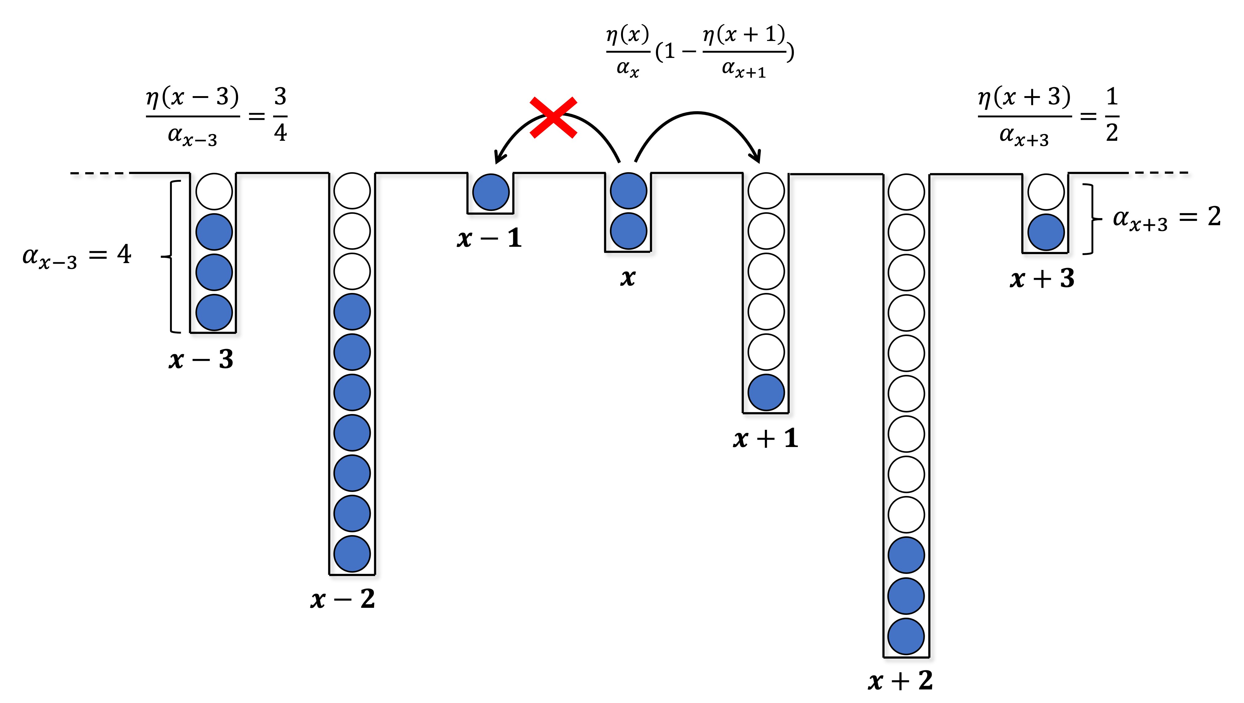
Figure 1. Schematic representation of the interacting system of ${\rm BTM}(a)$ on ${\mathbb{Z}}$ for a given realization of the environment, and with $a=0$. In each site $y\in{\mathbb{Z}}$, there is a trap of size $\alpha_{y}$; when the trap is full, no particles are allowed to jump there.

1.3. Main results

Denote by ${\mathbb{P}}_{\eta}$ the quenched law of the interacting particle system above when starting from $\eta$. The main results of the paper, Theorems 2.1 and 2.5, concern the behavior of the empirical density field of $\eta_{t}$ rescaled in space and time, for some $\theta_{n}\in(0,\infty)$ (cf. (2.7)), as follows:

$$\mathcal{X}^{n}_{t}=\frac{1}{n^{d/\beta}}\sum_{x\in{\mathbb{Z}}^{d}}\eta_{t\theta_{n}}(x)\,\delta_{x/n}\ .$$

Interestingly, the scaling and the limiting behavior change with the dimension.

Let $d\geq 3$, and set $\theta_{n}=\theta_{n,\beta,d\geq 3}:=n^{2/\beta}$. Fix a macroscopic profile, that is, a continuous function $\bar{\rho}:{\mathbb{R}}^{d}\to[0,1]$; furthermore, for every collection $\alpha=(\alpha_{x})_{x\in{\mathbb{Z}}^{d}}$ and $n\in{\mathbb{N}}$, let the process $\eta_{t}$ be initialized at $t=0$ according to the local equilibrium measure $\mu_{n}=\otimes_{x\in{\mathbb{Z}}^{d}}\,{\rm Bin}(\alpha_{x},\bar{\rho}(x/n))$. Then, under ${\mathbb{Q}}(\text{d}\alpha)\mu_{n}(\text{d}\eta){\mathbb{P}}_{\eta}$, the empirical density field $(\mathcal{X}^{n}_{t})_{t\geq 0}$ converges in distribution (w.r.t. a suitable topology) as $n\to\infty$ to $(\rho_{t}\mathcal{W})_{t\geq 0}$, $\rho_{t}\mathcal{W}(\text{d}x)=\rho_{t}(x)\mathcal{W}(\text{d}x)$, where:

• $\mathcal{W}$ is the random measure on ${\mathbb{R}}^{d}$ given by

  $$\mathcal{W}=\mathcal{W}_{\beta}:=\sum_{i}v_{i}\,\delta_{x_{i}}\ ,$$ (1.4)

  with $(v_{i},x_{i})_{i}$ being the support of a Poisson point process on $(0,\infty)\times{\mathbb{R}}^{d}$ with intensity measure $\beta v^{-(1+\beta)}\text{d}v\text{d}x$;

• $(\rho_{t})_{t\geq 0}$ is deterministic and solves, on ${\mathbb{R}}^{d}$,

  $$\frac{\partial^{\beta}}{\partial t^{\beta}}\rho_{t}=D_{\mathrm{eff}}\Delta\rho_{t}\ ,\quad\text{with}\ \rho_{0}=\bar{\rho}\ ,$$ (1.5)

  where $D_{\mathrm{eff}}=D_{\mathrm{eff}}({\mathbb{Q}},a,d)\in(0,\infty)$ does not depend on the specific realization of the environment $\alpha$.

Equation (1.5) — with the fractional derivative in time of order $\beta\in(0,1)$ meant in the Caputo sense (see (2.11) below) — is a well-studied time-fractional sub-diffusive PDE, known as fractional kinetics equation (FKE), e.g., [10]. In words, our main result states that the HL of the partial exclusion process in a heavy-tailed random environment, when sub-diffusively rescaled, is a random measure, absolutely continuous with respect to $\mathcal{W}$ in (1.4) and whose density is deterministic and solves the FKE. As we show in Theorem 2.1 below, an analogous result holds in dimension $d=2$, but time has to be rescaled differently. In fact, the same result holds for

$$\frac{1}{n^{2/\beta}}\sum_{x\in{\mathbb{Z}}^{d}}\eta_{t\theta_{n}}(x)\,\delta_{x/n}\ ,\qquad\theta_{n}=\theta_{n,\beta,d=2}:=n^{2/\beta}(\log n)^{1-1/\beta}\ .$$

We emphasize that, while the macroscopic evolution is purely deterministic, the randomness of the environment still survives in the reference measure. This is not the case if one looks at the scaling behavior of a different field, which we refer to as the frequency field, defined as

$$\mathcal{Z}^{n}_{t}:=\frac{1}{n^{d}}\sum_{x\in{\mathbb{Z}}^{d}}\frac{\eta_{t\theta_{n}}(x)}{\alpha_{x}}\,\delta_{x/n}\ .$$

The fields $\mathcal{Z}^{n}_{t}$ converge to a deterministic measure absolutely continuous with respect to the Lebesgue measure and density given by $\rho_{t}$ described above; see Proposition 2.6 below.

We also analyze the one-dimensional case in Theorem 2.1 below and find a much different behavior which involves both different rescaling and limiting equation. Namely, under ${\mathbb{Q}}(\text{d}\alpha)\mu_{n}(\text{d}\eta){\mathbb{P}}_{\eta}$,

$$\frac{1}{n^{1/\beta}}\sum_{x\in{\mathbb{Z}}^{d}}\eta_{t\theta_{n}}(x)\,\delta_{x/n}\ ,\qquad\theta_{n}=\theta_{n,\beta,d=1}:=n^{1+1/\beta}\ ,$$

converges in distribution (w.r.t. a suitable topology) as $n\to\infty$ to $(\rho_{t}\mathcal{W})_{t\geq 0}$, where $\mathcal{W}$ is the same as before but now $\rho_{t}$ is random and solves, on ${\mathbb{R}}$,

$$\frac{\partial}{\partial t}\rho_{t}(x)=\frac{\partial}{\partial\mathcal{W}}\frac{\partial}{\partial x}\rho_{t}(x)\ ,\quad\text{with}\ \rho_{0}=\bar{\rho}\ ,$$ (1.6)

where $\frac{df}{d\mathcal{W}}=g$ has to be interpreted as

$$f(x)=c+\int_{-\infty}^{x}g(z)\,\mathcal{W}(\text{d}z)\ ,\quad x\in{\mathbb{R}}\ ,$$ (1.7)

for some $c\in{\mathbb{R}}$.

1.4. Comparison with the literature

The only interacting system which has been shown to rescale to a sub-diffusive equation is SSEP with i.i.d. conductances satisfying, for some $\beta\in(0,1)$,

$${\mathbb{Q}}(\omega_{xy}^{-1}>u)=u^{-\beta}(1+o(1))\ ,\quad\text{as}\ u\to\infty\ .$$

When properly rescaling the empirical density fields, it has been proven for $d=1$ in [20] (see [24, 39] for the more general case with $d\geq 1$) that the HL is given by

$$\frac{\partial}{\partial t}\rho_{t}(x)=\frac{\partial}{\partial x}\frac{\partial}{\partial W}\rho_{t}(x)\ ,\quad x\in{\mathbb{R}}\ ,$$

where $W$ is a random càdlàg function with heavy-tailed jumps of parameter $\beta$, and $\frac{df}{dW}=g$ is interpreted as in (1.7) with $W$ in place of $\mathcal{W}$; for further details, we refer the interested reader to [20].

From the point of view of one-particle models, the literature on random walks converging to sub-diffusive processes is vast, and a prominent place is taken by the ${\rm BTM}$ (see [5], and references therein). Scaling limits of ${\rm BTM}$ have been studied (see, e.g., [23, 4, 2, 9]), and the limiting processes are the so-called Fontes-Isopi-Newman (FIN) diffusion in $d=1$, and the fractional kinetics process in $d\geq 2$.

The article [30] is the only one dealing with rigorous scaling limits for systems of many ${\rm BTM}$. There, the authors consider a system of independent symmetric particles of this kind and, in $d=1$, obtain (1.6) as a HL, i.e., the same HL that arises for the one-dimensional partial exclusion process in a heavy-tailed random environment as considered in this paper.

Interacting ${\rm BTM}$ have not been studied so far: our model is the first example in this direction and it has the advantage of still satisfying stochastic duality.

1.5. Organization of the paper

The rest of the paper is organized as follows. In §2, we rigorously state the main results. The remaining three sections, §3, §4 and §5, are devoted to the proof of our main results. In Appendix A we provide a construction of the particle system based on duality.

2. Main results

Here and all throughout ${\mathbb{N}}=\{1,2,\ldots\}$, $\mathcal{C}_{b}({\mathbb{R}}^{d})$ denotes the space of continuous and bounded functions on ${\mathbb{R}}^{d}$, $\mathcal{C}_{c}^{+}({\mathbb{R}}^{d})$ its subspace of non-negative functions with compact support, while $\mathcal{M}_{v}({\mathbb{R}}^{d})=(\mathcal{M}_{loc}({\mathbb{R}}^{d}),\tau_{v})$ denotes the space of locally finite measures on ${\mathbb{R}}^{d}$ endowed with the vague topology $\tau_{v}$, i.e., the weakest topology on $\mathcal{M}_{loc}({\mathbb{R}}^{d})$ for which all mappings $\nu\in\mathcal{M}_{loc}({\mathbb{R}}^{d})\mapsto\langle\nu|f\rangle:=\int_{{\mathbb{R}}^{d}}f(x)\,\nu(\text{d}x)\in{\mathbb{R}}$, $f\in\mathcal{C}_{c}^{+}({\mathbb{R}}^{d})$, are continuous. All throughout, we write “$Y^{n}\underset{n\to\infty}{\Longrightarrow}Y$”  for convergence in distribution of real-valued random variables $Y^{n},Y\in{\mathbb{R}}$, while “$\mathcal{Y}^{n}\underset{n\to\infty}{\Longrightarrow}\mathcal{Y}$ in $\mathcal{M}_{v}({\mathbb{R}}^{d})$” for convergence in distribution of random measures $\mathcal{Y}^{n},\mathcal{Y}\in\mathcal{M}_{v}({\mathbb{R}}^{d})$, i.e.,

$$\mathcal{Y}^{n}\underset{n\to\infty}{\Longrightarrow}\mathcal{Y}\quad{\rm in}\ \mathcal{M}_{v}({\mathbb{R}}^{d})\qquad\text{if}\qquad\langle\mathcal{Y}^{n}|f\rangle\underset{n\to\infty}{\Longrightarrow}\langle\mathcal{Y}|f\rangle\ \text{for all}\ f\in\mathcal{C}^{+}_{c}({\mathbb{R}}^{d})\ .$$ (2.1)

Let us first introduce the underlying random environment. Fix $\beta\in(0,1)$ and $d\geq 1$. Recall from (1.4) the definition of the random measure

$$\mathcal{W}=\mathcal{W}_{\beta}:=\sum_{i}v_{i}\,\delta_{x_{i}}\in\mathcal{M}_{v}({\mathbb{R}}^{d})\ ,$$ (2.2)

generated by the Poisson point process $((v_{i},x_{i}))_{i}$ on $(0,\infty)\times{\mathbb{R}}^{d}$ with intensity measure $\beta v^{-(\beta+1)}\text{d}v\text{d}x$. We define, for all $n\in{\mathbb{N}}$,

$$\mathcal{W}^{n}=\mathcal{W}^{n}_{\beta}:=\frac{1}{n^{d/\beta}}\sum_{x\in{\mathbb{Z}}^{d}}\alpha_{x}\,\delta_{x/n}\in\mathcal{M}_{v}({\mathbb{R}}^{d})\ ,$$ (2.3)

where $(\alpha_{x})_{x\in{\mathbb{Z}}^{d}}$ is a collection of ${\mathbb{N}}$-valued i.i.d. random variables with product law ${\mathbb{Q}}={\mathbb{Q}}_{\beta}$ whose marginals satisfy

$${\mathbb{Q}}\big{(}\alpha_{0}>u\big{)}=u^{-\beta}\left(1+o(1)\right)\ ,\quad\text{as}\ u\to\infty\ .$$ (2.4)

By inspection of the moment generating functions, the following convergence in distribution in $\mathcal{M}_{v}({\mathbb{R}}^{d})$ holds (see, e.g., [13, Lem. 5.3]):

$$\mathcal{W}^{n}\underset{n\to\infty}{\Longrightarrow}\mathcal{W}\ \quad\text{in}\ \mathcal{M}_{v}({\mathbb{R}}^{d})\ .$$ (2.5)

Before presenting the interacting particle system, we recall the definition of a single ${\rm BTM}$, and some of its main properties.

2.1. ${\rm BTM}$ and its scaling limits

Fix $a\in[0,1]$. Given ${\mathbb{Q}}$ satisfying (2.4), the Bouchaud trap model with parameter $a\in[0,1]$ (${\rm BTM}(a)$) in the environment $\alpha$ sampled according to ${\mathbb{Q}}$, is the continuous-time random walk $(X_{t})_{t\geq 0}$ on ${\mathbb{Z}}^{d}$ with infinitesimal generator given in (1.2). Note that $A$ is symmetric in $L^{2}(\mathcal{W}^{n})$ with $n=1$. In what follows, $\mathbf{P}^{\alpha}_{x}$ and $\mathbf{E}^{\alpha}_{x}$ denote the quenched law and corresponding expectation of $X_{t}$ when $X_{0}=x\in{\mathbb{Z}}^{d}$.

We are mainly interested in the scaling properties of ${\rm BMT}(a)$. For this purpose, let, for all $n\in{\mathbb{N}}$ and continuous and bounded functions $g\in\mathcal{C}_{b}({\mathbb{R}}^{d})$,

$$P^{n}_{t}g(x/n):=\mathbf{E}^{\alpha}_{x}\left[g(X_{t\theta_{n}}/n)\right]\ ,\qquad x\in{\mathbb{Z}}^{d}\ ,\ t\geq 0\ ,$$ (2.6)

denote the semigroup of a sub-diffusive rescaling of $X_{t}$, where space has been shrunk by a factor $1/n$, and time sped-up by the following amount:

$$\theta_{n}=\theta_{n,\beta,d}:=\begin{cases}n^{2/\beta}&\text{if}\ d\geq 3\\ n^{2/\beta}\left(\log n\right)^{1-1/\beta}&\text{if}\ d=2\\ n^{1+1/\beta}&\text{if}\ d=1\ .\end{cases}$$ (2.7)

As we will discuss in §3.2, there exists some strictly positive constant $\kappa=\kappa({\mathbb{Q}},\beta,a,d)$ which does not depend on the realization of the environment for which $P^{n}_{t}$ converges, in a suitable sense, to $\mathcal{P}_{\kappa t}$ as $n\to\infty$, where for every $g\in\mathcal{C}_{b}({\mathbb{R}}^{d})$, $g_{t}:=\mathcal{P}_{t}g$ solves the following PDEs, on ${\mathbb{R}}^{d}$,

$$\frac{\partial}{\partial t}g_{t}(x)=\frac{\partial}{\partial\mathcal{W}}\frac{\partial}{\partial x}g_{t}(x)\ ,\qquad d=1\ ,$$ (2.8)

$$\frac{\partial^{\beta}}{\partial t^{\beta}}g_{t}(x)=\Delta g_{t}(x)\ ,\qquad d\geq 2\ ,$$ (2.9)

with $g_{0}=g$. We recall that one writes $\frac{\partial}{\partial\mathcal{W}}\frac{\partial}{\partial x}f=h$ if

$$f(x)=c_{1}+c_{2}x+\int_{0}^{x}\int_{0}^{y}h(z)\mathcal{W}(\text{d}z)\,\text{d}y\ ,\qquad x\in{\mathbb{R}}\ ,$$ (2.10)

holds for some $c_{1},c_{2}\in{\mathbb{R}}$, while $\frac{\partial^{\beta}}{\partial t^{\beta}}$ is meant in the Caputo sense (e.g., [10, Eq. (1.1)]):

$$\frac{\partial^{\beta}}{\partial t^{\beta}}f(t):=\frac{1}{\Gamma(1-\beta)}\int_{0}^{t}\frac{1}{(t-s)^{\beta}}f^{\prime}(s)\,\text{d}s\ ,\qquad t\geq 0\ ,\ f\in\mathcal{C}^{1}({\mathbb{R}})\ .$$ (2.11)

Interestingly, $(\mathcal{P}_{t})_{t\geq 0}$ admits a stochastic representation:

• for $d=1$, it is the (random) Markov semigroup of the ${\rm FIN}$ diffusion $(Z(t))_{t\geq 0}$ of parameter $\beta\in(0,1)$ associated to the random measure $\mathcal{W}=\mathcal{W}_{\beta}$ in (1.4);

• for $d\geq 2$, it is the pseudo-semigroup of the semi-Markov process $(FK_{\beta}(t))_{t\geq 0}$ known as fractional kinetics process of parameter $\beta\in(0,1)$.

More precisely, letting $B=(B(t))_{t\geq 0}$ denote the $d$-dimensional Brownian motion, for $d=1$, the FIN diffusion with parameter $\beta\in(0,1)$ is given by

$$Z(s):=B(\psi^{-1}(s))\ ,\qquad s\geq 0\ ,$$ (2.12)

where $\psi{{}^{-1}}$ denotes the generalized right inverse of $t\mapsto\psi(t):=\int_{\mathbb{R}}\ell(t,x)\mathcal{W}(\text{d}x)$, with $\ell(t,x)$ being the local time of $B(t)$ at $x\in{\mathbb{R}}$. In other words, $Z$ is a diffusion process (actually, often referred to as a quasi- or singular diffusion, see, e.g., [5]) expressed as a time change of a standard one-dimensional Brownian motion with speed measure $\mathcal{W}$. As for $FK_{\beta}$ in $d\geq 2$, we have

$$FK_{\beta}(t):=B(V_{\beta}^{-1}(t))\ ,\qquad t\geq 0\ ,$$ (2.13)

where $V_{\beta}$ stands for a $\beta$-stable subordinator independent of $B$, and $V_{\beta}^{-1}(t):=\inf\{s\geq 0:V_{\beta}(s)>t\}$. Finally, we remark that both processes introduced above are sub-diffusive, i.e., their mean square displacement behaves as

$$E[Z(t)^{2}]=t^{2\beta/(1+\beta)}\quad\text{and}\quad E[FK_{\beta}(t)^{2}]=t^{\beta}\ ,\qquad t\geq 0\ .$$

For further properties of $Z(t)$ and $FK_{\beta}(t)$, we refer the interested reader to [5, §§3,4] and references therein.

2.2. Interacting particle system

Recall the interacting system of ${\rm BTM}(a)$ with generator given in (1.3). The infinite particle system $\eta_{t}$ turns out to be well-defined, ${\mathbb{Q}}$-a.s., for all times and initial configurations. A proof of this fact may be extracted from the very same percolation arguments in [2] employed within the context of the single-particle system: these yield a well-defined, ${\mathbb{Q}}$-a.s., graphical representation for $\eta_{t}$ as, e.g., in [22, App. A]. Instead of detailing this rather standard approach (see, e.g., [17, 35]), in Appendix §A below, we discuss an alternative construction of the infinite system solely based on self-duality, which may be of independent interest and applicable to other interacting particle systems, such as the symmetric inclusion process (see, e.g., [26]).

Fix a realization of $(\alpha_{x})_{x\in{\mathbb{Z}}^{d}}$. For a probability measure $\mu$ on $\Xi$, ${\mathbb{P}}^{\alpha}_{\mu}$ and ${\mathbb{E}}^{\alpha}_{\mu}$ denote the law and corresponding expectation, respectively, of the particle system $\eta_{t}$ such that $\eta_{0}\sim\mu$. By a detailed balance computation, it is not difficult to show that, for every $\rho\in[0,1]$, the product measure $\nu_{\rho}:=\otimes_{x\in{\mathbb{Z}}^{d}}\,{\rm Bin}(\alpha_{x},\rho)$ is reversible for $\eta_{t}$.

2.3. Hydrodynamic limit

In order to present our main result, we introduce:

1. a reference profile $\rho_{0}\in\mathcal{C}_{b}({\mathbb{R}}^{d})$, $\rho_{0}\in[0,1]$;

2. the empirical density fields associated to the sub-diffusive rescaling of $\eta_{t}$ as in (2.6):

   $$t\in[0,\infty)\longmapsto\mathcal{X}^{n}_{t}:=\frac{1}{n^{d/\beta}}\sum_{x\in{\mathbb{Z}}^{d}}\eta_{t\theta_{n}}(x)\,\delta_{x/n}\in\mathcal{M}_{v}({\mathbb{R}}^{d})\ ,$$ (2.14)

   where $\theta_{n}$ is defined in (2.7);

3. the random measures $\rho_{t}\mathcal{W}(\text{d}x):=\rho_{t}(x)\mathcal{W}(\text{d}x)$ in $\mathcal{M}_{v}({\mathbb{R}}^{d})$, where $\mathcal{W}$ is given in (1.4), and $\rho_{t}:=\mathcal{P}_{\kappa t}\rho_{0}$, for $\kappa=\kappa({\mathbb{Q}},\beta,a,d)>0$ as given in Proposition 3.4 below.

Recall (2.1). We now present the main result of the paper: roughly speaking, it asserts that, if $\mathcal{X}^{n}_{0}\Longrightarrow\rho_{0}\mathcal{W}$ in $\mathcal{M}_{v}({\mathbb{R}}^{d})$, then the same convergence holds for all later times.

Theorem 2.1 (Hydrodynamic limit, §3).

Let $d\geq 1$ and $a\in[0,1]$. For all $n\in{\mathbb{N}}$, let $\mu_{n}=\otimes_{x\in{\mathbb{Z}}^{d}}\,{\rm Bin}(\alpha_{x},\rho_{0}(x/n))$ be the initial distribution of the particle system. Then, for all $t\geq 0$, $\mathcal{X}^{n}_{t}\underset{n\to\infty}{\Longrightarrow}\rho_{t}\mathcal{W}$ in $\mathcal{M}_{v}({\mathbb{R}}^{d})$.

The above theorem holds under slightly more general assumptions on the sequence of initial distributions $\mu_{n}$, namely Assumptions 2.2 and 2.3 below. In what follows, for $x\in{\mathbb{Z}}^{d}$, $t\geq 0$ and $\mu_{n}$ a probability distribution on $\Xi$, we set

$$D^{n}_{t}(x/n):=\eta_{t\theta_{n}}(x)/\alpha_{x}\ \quad\text{and}\quad\rho^{n}_{t}(x/n):={\mathbb{E}}_{\mu_{n}}\left[D^{n}_{t}(x/n)\right]\ .$$ (2.15)

Moreover, $\left\|f\right\|_{n,p}^{p}:=\langle\mathcal{W}^{n}||f|^{p}\rangle$ for $p\in[1,\infty)$, while $\left\|f\right\|_{n,\infty}:=\sup_{x\in{\mathbb{Z}}^{d}}\left|f(x/n)\right|$.

Assumption 2.2.

There exists $C>0$, $p,q\in[1,\infty]$, and a diverging sequence $(m_{n})_{n\in{\mathbb{N}}}$ such that the sequence of probability measures $(\mu_{n})_{n\in{\mathbb{N}}}$ on $\Xi$ satisfies, ${\mathbb{Q}}$-a.s.,

$${\mathbb{E}}_{\mu_{n}}\left[\left(\langle\mathcal{W}^{n}|\left(D^{n}_{0}-\rho^{n}_{0}\right)f\rangle\right)^{2}\right]\leq\frac{C}{m_{n}}\left\|f\right\|_{n,p}\left\|f\right\|_{n,q}\ ,\qquad f\in\mathcal{C}_{c}^{+}({\mathbb{R}}^{d})\ .$$

Assumption 2.3.

There exists $p_{0}\in[1,\infty]$ satisfying

$$\left\|\rho^{n}_{0}-\rho_{0}\right\|_{n,p_{0}}\underset{n\to\infty}{\Longrightarrow}0\ .$$

Remark 2.4.

Clearly, $\mu_{n}=\otimes_{x\in{\mathbb{Z}}^{d}}\,{\rm Bin}(\alpha_{x},\rho_{0}(x/n))$ satisfies Assumption 2.2 with $p=q=2$, $m_{n}=n^{-d/\beta}$, and trivially Assumption 2.3 for any $p_{0}\in[1,\infty]$ because $\rho_{0}^{n}=\rho_{0}$. Nonetheless, the above assumptions allow to consider initial distributions other than just slowly-varying product measures. Another example of sequence $\mu_{n}$ satisfying Assumptions 2.2 and 2.3 consists of an independent patching of non-equilibrium steady states with Lipschitz boundaries and uniformly continuous boundary condition given by $\rho_{0}$ considered in [15]; more precisely, Lemma 7.10 in [15] ensures that Assumption 2.2 holds with $p=1,q=\infty$, and $m_{n}=n^{-d/\beta}$, while, by Theorem 3.2 therein, Assumption 2.3 holds with $p_{0}=\infty$.

It is not difficult to extract from the proof of Theorem 2.1 convergence of all finite-dimensional distributions of $\mathcal{X}^{n}_{t}$, i.e., for all $k\in{\mathbb{N}}$ and $0\leq t_{1}<\ldots<t_{k}$,

$$\left(\mathcal{X}^{n}_{t_{1}},\ldots,\mathcal{X}^{n}_{t_{k}}\right)\underset{n\to\infty}{\Longrightarrow}\left(\rho_{t_{1}}\mathcal{W},\ldots,\rho_{t_{k}}\mathcal{W}\right)\quad\text{in}\ \mathcal{M}_{v}({\mathbb{R}}^{d})^{\otimes k}\ .$$ (2.16)

Theorem 2.1 is strengthened in the following result, from which a pathwise hydrodynamic limit follows. All throughout, for a Polish space $E$, $\mathcal{D}([0,\infty);E)$ denotes the space of càdlàg $E$-valued paths endowed with the $J_{1}$-Skorokhod topology (see, e.g., [6]). Recall that $\mathcal{M}_{v}({\mathbb{R}}^{d})$ is Polish (see, e.g., [31, Th. A5.5]).

Theorem 2.5 (Tightness, §4).

Let $d\geq 1$ and $a\in[0,1]$. Then, for all $(\mu_{n})_{n\in{\mathbb{N}}}$ initial distributions for $\eta_{t}$ satisfying Assumption 2.2 and 2.3, the sequence $(\mathcal{X}^{n}_{\cdot})_{n\in{\mathbb{N}}}$ admits a càdlàg version which is tight in $\mathcal{D}([0,\infty);\mathcal{M}_{v}({\mathbb{R}}^{d}))$.

2.4. Empirical frequency fields

Theorem 2.1 asserts that, when considering the scaling limit of the sub-diffusively rescaled empirical density fields in the heavy-tailed random environment $(\alpha_{x})_{x\in{\mathbb{Z}}^{d}}$, randomness survives in the limit. Indeed, although $\rho_{t}$ is ${\mathbb{Q}}$-a.s. constant for $d\geq 2$, the reference measure $\mathcal{W}$ is random for all $d\geq 1$. In other words, $\mathcal{X}^{n}_{t}$ does not fully homogenize in the limit. We are thus left with the question whether by choosing different observables of the infinite particle system, one recovers $\rho_{t}{\rm Leb}_{{\mathbb{R}}^{d}}$ in place of $\rho_{t}\mathcal{W}$ as a HL, with ${\rm Leb}_{{\mathbb{R}}^{d}}$ denoting the Lebesgue measure: in other words, whether the randomness disappears in the reference measure.

We, thus, consider the following rescaled empirical frequency fields:

$$t\in[0,\infty)\longmapsto\mathcal{Z}^{n}_{t}:=\frac{1}{n^{d}}\sum_{x\in{\mathbb{Z}}^{d}}\frac{\eta_{t\theta_{n}}(x)}{\alpha_{x}}\,\delta_{x/n}\in\mathcal{M}_{v}({\mathbb{R}}^{d})\ .$$ (2.17)

There are two main differences between such fields and the density fields $\mathcal{X}^{n}_{t}$ in (2.14). On the one hand, $\mathcal{Z}^{n}_{t}$ considers the frequency variables of occupied slots at each site, rather than the occupancy variables themselves; we remark that frequency as a standard observable appears extensively in the population genetics literature, where, e.g., sites represent colonies, particles individuals of type $A$, say, and holes individuals of type $a$ (see, e.g., [16]). On the other hand, for $\mathcal{Z}^{n}_{t}$, each Dirac delta is weighted by the most standard weight $n^{-d}$, the unit volume of a cube in ${\mathbb{R}}^{d}$ of size $1/n$. For such fields, we obtain:

Proposition 2.6 (§5).

Let $d\geq 1$ and $a\in[0,1]$. For all $n\in{\mathbb{N}}$, let $\otimes_{x\in{\mathbb{Z}}^{d}}\,{\rm Bin}(\alpha_{x},\rho_{0}(x/n))$ be the initial distribution $\mu_{n}$ of the particle system. Then, for every $t\geq 0$, $\mathcal{Z}^{n}_{t}\underset{n\to\infty}{\Longrightarrow}\rho_{t}{\rm Leb}_{{\mathbb{R}}^{d}}$ in $\mathcal{M}_{v}({\mathbb{R}}^{d})$.

Recall $D^{n}_{t}(x/n)$ from (2.15). Note that the fields $\mathcal{X}^{n}_{t}$ and $\mathcal{Z}^{n}_{t}$ read as

$$\mathcal{X}^{n}_{t}=\frac{1}{n^{d/\beta}}\sum_{x\in{\mathbb{Z}}^{d}}\alpha_{x}\,D^{n}_{t}(x/n)\,\delta_{x/n}\ ,\qquad\mathcal{Z}^{n}_{t}=\frac{1}{n^{d}}\sum_{x\in{\mathbb{Z}}^{d}}D^{n}_{t}(x/n)\,\delta_{x/n}\ ,$$

Hence, reconsidering Theorem 2.1 in light of Proposition 2.6, we have that, for $d\geq 2$, only the dynamic quantity $D^{n}_{t}$ homogenizes converging to $\rho_{t}$ as $n\to\infty$, while the underlying reference measure $\frac{1}{n^{d/\beta}}\sum_{x\in{\mathbb{Z}}^{d}}\alpha_{x}\,\delta_{x/n}$ in $\mathcal{X}^{n}_{t}$ does not.

3. Proof of Theorem 2.1

In this section we prove the main theorem of the article, Theorem 2.1, assuming that the initial distributions $\mu_{n}$ satisfy Assumptions 2.2 and 2.3. In order to prove the theorem, we decompose the empirical density fields $\mathcal{X}^{n}_{t}$, for all $t>0$ and test functions $f\in\mathcal{C}_{c}^{+}({\mathbb{R}}^{d})$, as follows:

$$\langle\mathcal{X}^{n}_{t}|f\rangle:=\frac{1}{n^{d/\beta}}\sum_{x\in{\mathbb{Z}}^{d}}\eta_{t\theta_{n}}(x)\,f(x/n)$$

$$=\frac{1}{n^{d/\beta}}\sum_{x\in{\mathbb{Z}}^{d}}\left(\eta_{t\theta_{n}}(x)-{\mathbb{E}}_{\eta_{0}}\left[\eta_{t\theta_{n}}(x)\right]\right)f(x/n)$$

$$\qquad+\frac{1}{n^{d/\beta}}\sum_{x\in{\mathbb{Z}}^{d}}\alpha_{x}\left({\mathbb{E}}_{\eta_{0}}\left[\eta_{t\theta_{n}}(x)/\alpha_{x}\right]-P^{n}_{t}\rho^{n}_{0}(x/n)\right)f(x/n)$$

$$\qquad+\frac{1}{n^{d/\beta}}\sum_{x\in{\mathbb{Z}}^{d}}\alpha_{x}\left(P^{n}_{t}\rho^{n}_{0}(x/n)-P^{n}_{t}\rho_{0}(x/n)\right)f(x/n)$$

$$\qquad+\frac{1}{n^{d/\beta}}\sum_{x\in{\mathbb{Z}}^{d}}\alpha_{x}\,P^{n}_{t}\rho_{0}(x/n)\,f(x/n)$$

$$=:{\rm I}_{n}+{\rm II}_{n}+{\rm III}_{n}+\langle P^{n}_{t}\rho_{0}\mathcal{W}^{n}|f\rangle\ .$$ (3.1)

It now suffices to show that:

Part I. All three terms ${\rm I}_{n}$, ${\rm II}_{n}$, and ${\rm III}_{n}$ vanish in distribution (of the environment, jointly with that of the particle system) as $n\to\infty$;

Part II. The last term $\langle P^{n}_{t}\rho_{0}\mathcal{W}^{n}|f\rangle$ converges in distribution to $\langle\mathcal{P}_{ct}\rho_{0}\mathcal{W}|f\rangle$.

We prove the first one of these claims in §3.1, while the second one (i.e., (3.12) below) in §3.2. In the remainder of the paper, we will make use of the stochastic self-duality satisfied by the interacting particle system under consideration (see, e.g., [37, 26, 36, 22, 21]) with respect to the duality functions (cf. (2.15))

$$D(x)=D(x,\eta):=\frac{\eta(x)}{\alpha_{x}}\quad\text{and}\quad D(x,y)=D((x,y),\eta):=\frac{\eta(x)}{\alpha_{x}}\frac{\eta(y)-\mathbbm{1}_{x}(y)}{\alpha_{y}-\mathbbm{1}_{x}(y)}\ ;$$

More precisely, ${\mathbb{Q}}$-a.s., for all $t\geq 0$, $\eta\in\Xi$, and $x,y\in{\mathbb{Z}}^{d}$, the following relations hold:

$${\mathbb{E}}_{\eta}\left[\eta_{t}(x)\right]=\alpha_{x}\,P_{t}D(x)\ ,$$ (3.2)

and

$${\mathbb{E}}_{\eta}\left[\eta_{t}(x)(\eta_{t}(y)-\mathbbm{1}_{x}(y))\right]=\alpha_{x}({\alpha_{y}-\mathbbm{1}_{x}(y)})\,P^{(2)}_{t}D(x,y)\ ,$$ (3.3)

where $P_{t}:=P_{t}^{n}$ for $n=1$ denotes the semigroup of ${\rm BTM}(a)$ with generator given in (1.2), while $P^{(2)}_{t}$ the semigroup of the position of two interacting ${\rm BTM}(a)$ evolving according to the generator given in (1.3); the corresponding space-time rescaled versions $P^{n}_{t}$ and $P^{(2),n}_{t}$ are readily obtained (cf. (2.6)).

3.1. Proof of Theorem 2.1. Part I

3.1.1. A variance estimate

We start by proving an auxiliary result. By knowing first and second moments of the empirical density fields $\mathcal{X}^{n}_{t}$, and by the negative dependence of the partial symmetric exclusion process, we readily obtain the following variance estimate:

Proposition 3.1.

${\mathbb{Q}}$-a.s., for all $\eta\in\Xi$, $t\geq 0$, $n\in{\mathbb{N}}$, and $f\in\mathcal{C}^{+}_{c}({\mathbb{R}}^{d})$,

$${\mathbb{E}}_{\eta}\left[\left(\langle\mathcal{X}^{n}_{t}|f\rangle-\langle\mathcal{X}^{n}_{0}|P^{n}_{t}f\rangle\right)^{2}\right]\leq\frac{1}{n^{d/\beta}}\langle\mathcal{X}^{n}_{0}|P^{n}_{t}(f^{2})-\left(P^{n}_{t}f\right)^{2}\rangle\ .$$ (3.4)

Proof.

Abbreviate with $\gamma:=d/\beta$. Writing $\eta_{t}(x,y):=\eta_{t}(x)\left(\eta_{t}(y)-\mathbbm{1}_{x}(y)\right)$, we get

$$\begin{aligned} &{\mathbb{E}}_{\eta}\left[\left(\mathcal{X}^{n}_{t}(f)-\mathcal{X}^{n}_{0}(P^{n}_{t}f)\right)^{2}\right]\\ &=\frac{1}{n^{2\gamma}}\sum_{x,y\in{\mathbb{Z}}^{d}}f(x/n)f(y/n)\left({\mathbb{E}}_{\eta}\left[\eta_{t\theta_{n}}(x,y)\right]-{\mathbb{E}}_{\eta}\left[\eta_{t\theta_{n}}(x)\right]{\mathbb{E}}_{\eta}\left[\eta_{t\theta}(y)\right]\right)\\ &\qquad+\frac{1}{n^{2\gamma}}\sum_{x\in{\mathbb{Z}}^{d}}f(x/n)^{2}\,{\mathbb{E}}_{\eta}\left[\eta_{t\theta_{n}}(x)\right]\ .\end{aligned}$$ (3.5)

Using (3.2) and symmetry of $P_{t}^{n}$ in $L^{2}(\mathcal{W}^{n})$, the second term on the right-hand side of (3.5) equals $\frac{1}{n^{\gamma}}\langle\mathcal{X}^{n}_{0}|P_{t}^{n}(f^{2})\rangle$, i.e., the term $\frac{1}{n^{\gamma}}\langle\mathcal{X}^{n}_{0}|P^{n}_{t}(f^{2})\rangle$ on the right-hand side of (3.4). After a simple manipulation, the first term on the right-hand side of (3.5) reads as follows:

$$\frac{1}{n^{2\gamma}}\sum_{x,y\in{\mathbb{Z}}^{d}}(P^{(2),n}_{t}-(P^{n}_{t}\otimes P^{n}_{t}))(f\otimes f)(x/n,y/n)\,\eta_{0}(x,y)$$ (3.6)

$$\qquad-\frac{1}{n^{2\gamma}}\sum_{x\in{\mathbb{Z}}^{d}}(P^{n}_{t}f(x/n))^{2}\eta_{0}(x)\ .$$

Note that the second term in (3.6) corresponds to $-\frac{1}{n^{\gamma}}\langle\mathcal{X}^{n}_{0}|(P^{n}_{t}f)^{2}\rangle$, i.e., the remaining term on the right-hand of (3.4). We conclude by showing that the first term in (3.6) is non-positive; for notational convenience, we only show this for $n=1$. Letting $A\oplus A$ and $A^{(2)}$ denote the Markov generators of $P_{t}\otimes P_{t}$ and $P^{(2)}_{t}$, respectively, by integration-by-parts, we get

$$(P^{(2)}_{t}-(P_{t}\otimes P_{t}))(f\otimes f)(x,y)$$

$$=\int_{0}^{t}P^{(2)}_{t-s}\left(A^{(2)}-A\oplus A\right)(P_{s}f\otimes P_{s}f)(x,y)\,\text{d}s$$

$$=\sum_{z,w\in{\mathbb{Z}}^{d}}\int_{0}^{t}P^{(2)}_{t-s}\mathbbm{1}_{(z,w)}(x,y)\,\left(A^{(2)}-A\oplus A\right)\left(P_{s}f\otimes P_{s}f\right)(z,w)\,\text{d}s$$

$$=-\theta_{n=1}\sum_{z\sim w}\alpha_{z}^{a-1}\alpha_{w}^{a-1}\int_{0}^{t}\left(P^{(2)}_{t-s}\mathbbm{1}_{\{z,w\}}(x,y)\right)\left(P_{s}f(z)-P_{s}f(w)\right)^{2}\text{d}s$$

$$\leq 0\ .$$

Since $\eta_{0}(x,y)\geq 0$, we get the desired claim:

$$\sum_{x,y\in{\mathbb{Z}}^{d}}\big{(}P^{(2)}_{t}-P_{t}\otimes P_{t}\big{)}(f\otimes f)(x,y)\,\eta_{0}(x,y)\leq 0\ .$$

This concludes the proof. ∎

3.1.2. Vanishing of ${\rm I}_{n}$, ${\rm II}_{n}$, and ${\rm III}_{n}$

We now prove ${\rm I}_{n},{\rm II}_{n},{\rm III}_{n}\Longrightarrow 0$ as $n\to\infty$.

${\rm I}_{n}\Longrightarrow 0$ (dynamic noise). Fix $n\in{\mathbb{N}}$. Then, ${\mathbb{Q}}$-a.s., by (3.2) and Proposition 3.1, we get

$${\mathbb{E}}_{\mu_{n}}\left[\left({\rm I}_{n}\right)^{2}\right] \leq\frac{1}{n^{d/\beta}}\left\{\frac{1}{n^{d/\beta}}\sum_{x\in{\mathbb{Z}}^{d}}{\mathbb{E}}_{\mu_{n}}\left[\eta_{0}(x)\right]P^{n}_{t}(f^{2})(x/n)\right\}\leq\frac{1}{n^{d/\beta}}\,\langle\mathcal{W}^{n}|f^{2}\rangle\ .$$ (3.7)

Since $\langle\mathcal{W}^{n}|f^{2}\rangle\Longrightarrow\langle\mathcal{W}|f^{2}\rangle$ by (2.5) and $n^{-d/\beta}\to 0$, ${\rm I}_{n}$ vanishes in distribution.

${\rm II}_{n}\Longrightarrow 0$ (initial conditions’ variance). Fix $n\in{\mathbb{N}}$. Then, for ${\mathbb{Q}}$-a.e. $(\alpha_{x})_{x\in{\mathbb{Z}}^{d}}$, we have, by symmetry of $P^{n}_{t}$ with respect to $(\alpha_{x})_{x\in{\mathbb{Z}}^{d}}$,

$${\rm II}_{n}=\langle\mathcal{W}^{n}|\left(D^{n}_{0}-\rho^{n}_{0}\right)P^{n}_{t}f\rangle\ .$$

By Assumption 2.2 and $\left\|P^{n}_{t}f\right\|_{n,p}\leq\left\|f\right\|_{n,p}$, we have, ${\mathbb{Q}}$-a.s.,

$${\mathbb{E}}_{\mu_{n}}\left[\left({\rm II}_{n}\right)^{2}\right]\leq\frac{C}{m_{n}}\left\|P^{n}_{t}f\right\|_{n,p}\left\|P^{n}_{t}f\right\|_{n,q}\leq\frac{C}{m_{n}}\left\|f\right\|_{n,p}\left\|f\right\|_{n,q}\ ,$$

Since $f\in\mathcal{C}_{c}^{+}({\mathbb{R}}^{d})$, (2.5) ensures that $\left\|f\right\|_{n,p}\Longrightarrow\langle\mathcal{W}|\left|f\right|^{p}\rangle^{1/p}$, and similarly for $\left\|f\right\|_{n,q}$. Moreover, $m_{n}\to\infty$. Therefore, ${\rm II}_{n}$ vanishes in distribution as $n\to\infty$.

${\rm III}_{n}\Longrightarrow 0$ (initial conditions’ mean). Fix $n\in{\mathbb{N}}$. Then, ${\mathbb{Q}}$-a.s.,

$${\rm III}_{n}=\langle\mathcal{W}^{n}|\left(\rho^{n}_{0}-\rho_{0}\right)P^{n}_{t}f\rangle\ .$$

By Hölder inequality, ${\mathbb{Q}}$-a.s.,

$$\left|{\rm III}_{n}\right|\leq\left\|\rho^{n}_{0}-\rho_{0}\right\|_{n,p_{0}}\left\|P^{n}_{t}f\right\|_{n,q_{0}}\leq\left\|\rho^{n}_{0}-\rho_{0}\right\|_{n,p_{0}}\left\|f\right\|_{n,q_{0}}\ ,$$ (3.8)

where $p_{0}\in[1,\infty]$ is given in Assumption 2.3, and $q_{0}$ is its conjugate exponent. Finally, (2.5) and Assumption 2.3 ensure that ${\rm III}_{n}$ vanish in distribution as $n\to\infty$. This concludes Part I of the proof of Theorem 2.1.

Remark 3.2 (Quenched results).

If (2.5) and Assumption 2.3 held in a ${\mathbb{Q}}$-a.s. sense, then ${\rm I}_{n}$, ${\rm II}_{n}$ and ${\rm III}_{n}$ would vanish in a ${\mathbb{Q}}$-a.s. sense.

3.2. Proof of Theorem 2.1. Part II

Also for the proof of Part II, we need a preliminary result, specifically for the case $d\geq 2$. Namely, building on the quenched invariance principles for ${\rm BTM}(a)$, $a\in[0,1]$, when starting from the origin proved in [2, Thm. 1.3] (for $d\geq 3$) and [9, Thm. 1.2] (for $d=2$), we establish the following uniform convergence:

Proposition 3.3 (§3.3).

For all $d\geq 2$, there exists $\kappa=\kappa({\mathbb{Q}},\beta,a,d)>0$ satisfying, ${\mathbb{Q}}$-a.s.,

$$\lim_{n\to\infty}\sup_{\begin{subarray}{c}x\in{\mathbb{Z}}^{d}\\ x/n\in K\end{subarray}}\left|P^{n}_{t}g(x/n)-\mathcal{P}_{\kappa t}g(x/n)\right|=0\ ,\qquad g\in\mathcal{C}_{b}({\mathbb{R}}^{d})\ ,\ K\subset{\mathbb{R}}^{d}\ {\rm compact}\ .$$ (3.9)

We postpone the proof of this proposition to the next subsection, and present some quenched homogenization results required in our proof. We observe that, while such results hold ${\mathbb{Q}}$-a.s. when $d\geq 2$, for $d=1$ we provide an alternative construction of the underlying randomness.

Proposition 3.4.

For all $d\geq 1$, there exists a coupling $(\bar{}\mathcal{W},(\bar{\mathcal{P}}_{t})_{t\geq 0},(\bar{}\mathcal{W}^{n})_{n},((\bar{P}^{n}_{t})_{t\geq 0})_{n})$ with law $\bar{\mathbb{Q}}$ such that:

1. $\bar{}\mathcal{W}$ has the same law as $\mathcal{W}$, and similarly for all the other marginals; in particular, the following analogue of (2.5) holds:

   $$\langle\bar{}\mathcal{W}^{n}|f\rangle\underset{n\to\infty}{\Longrightarrow}\langle\bar{}\mathcal{W}|f\rangle\ ,\qquad f\in\mathcal{C}_{c}^{+}({\mathbb{R}}^{d})\ ;$$ (3.10)

2. for all $g\in\mathcal{C}_{b}({\mathbb{R}}^{d})$, $\bar{\mathcal{P}}_{t}g\bar{}\mathcal{W}$ has the same law as $\mathcal{P}_{t}g\mathcal{W}$, and similarly for $\bar{P}^{n}_{t}g\bar{}\mathcal{W}^{n}$;

3. $\bar{\mathbb{Q}}$-a.s., for all $g\in\mathcal{C}_{b}({\mathbb{R}}^{d})$ and $t\geq 0$, $\bar{}\mathcal{P}_{t}g:{\mathbb{R}}\to{\mathbb{R}}$ is continuous and bounded;

4. $\bar{\mathbb{Q}}$-a.s., for all $g\in\mathcal{C}_{b}({\mathbb{R}}^{d})$ and compact sets $K\subset{\mathbb{R}}^{d}$, $\left\|\mathbbm{1}_{K}\left(\bar{P}^{n}_{t}g-\bar{\mathcal{P}}_{\kappa t}g\right)\right\|_{n,\infty}\to 0$.

Further, if $d=1$:

1. $\bar{\mathbb{Q}}$-a.s., $\bar{}\mathcal{W}^{n}\to\bar{}\mathcal{W}$ in $\mathcal{M}_{v}({\mathbb{R}}^{d})$.

Proof.

For $d\geq 2$, we set $\bar{}\mathcal{W}^{n}:=\mathcal{W}^{n}$, $\bar{}\mathcal{P}_{t}:=\mathcal{P}_{t}$ constant (w.r.t. $\alpha$), and $\bar{}\mathcal{W}$ to be a copy of $\mathcal{W}$ independent of all $\mathcal{W}^{n}$. Then, items (1), (2), and (4) follow by (2.5) and Proposition 3.3; item (3) is a consequence of the heat kernel estimates in [11, Thm. 1.8].

For $d=1$, one possible coupling is the one given in [4, §§1–6]. Namely, first introduce the random locally finite measure $\bar{}\mathcal{W}$ ([4, p. 1172]). Conditional on $\bar{}\mathcal{W}$, define the Markov process $(\bar{Z}_{t}(x))_{t\geq 0,x\in{\mathbb{R}}}$, with $\bar{Z}_{0}(x)=x$, as in [4, Def. 1.1] (note that there is no problem in changing the starting point of the process, see, e.g., the end of [4, p. 1167]); to such a Markov process, associate its Markov semigroup $\bar{\mathcal{P}}_{t}$. By item (iv) in [5, Prop. 3.2], $\bar{\mathcal{P}}_{t}\rho_{0}:{\rm supp}(\bar{}\mathcal{W})\subset{\mathbb{R}}\to{\mathbb{R}}$ admits a unique continuous and bounded extension (see also [14]), which, by a slight abuse of notation, we keep calling $\bar{\mathcal{P}}_{t}$; this yields item (3). From the randomness used to generate $\bar{}\mathcal{W}$, construct, for every $n\in{\mathbb{N}}$, the random speed measure $\bar{}\mathcal{W}^{n}$, the random scale function $\bar{S}_{n}$, and the semigroups $\bar{P}^{n}_{t}$ and $\bar{P}^{n,\bar{S}_{n}}_{t}$ corresponding to the Markov jump processes evolving on ${\mathbb{Z}}_{n}:=\frac{{\mathbb{Z}}}{n}$ and on the tilted support $\bar{S}_{n}({\mathbb{Z}}_{n})\subset{\mathbb{R}}$ as in [4, p. 1172–3]. Such definitions immediately yield items (1), (2), and (5) of the proposition. Finally, by the first claim in [4, Prop. 6.2] — which generalizes as, e.g., in item (iv) of [4, Prop. 2.5], we get: conditional on $\bar{}\mathcal{W}$, for all $t>0$, $x\in{\mathbb{R}}$, and for all $(x_{n})_{n}$, $x_{n}\in{\mathbb{Z}}$, and $x_{n}/n\to x$,

$$\bar{P}^{n}_{t}g(x_{n}/n)\xrightarrow{n\to\infty}\bar{\mathcal{P}}_{\kappa t}g(x)\ ,\qquad\kappa=1\ .$$ (3.11)

By the space-continuity of $\bar{\mathcal{P}}_{\kappa t}g$, (3.11) is actually equivalent to item (4) of the proposition, thus, concluding the proof. ∎

In view of item (2) in Proposition 3.4, the claim

$$P^{n}_{t}\rho_{0}\mathcal{W}^{n}\underset{n\to\infty}{\Longrightarrow}{\mathcal{P}}_{\kappa t}\rho_{0}\mathcal{W}\ \quad\text{in}\ \mathcal{M}_{v}({\mathbb{R}}^{d})$$ (3.12)

is a consequence of the following:

Lemma 3.5.

For all $d\geq 1$, $\bar{P}^{n}_{t}\rho_{0}\bar{}\mathcal{W}^{n}\underset{n\to\infty}{\Longrightarrow}\bar{\mathcal{P}}_{\kappa t}\rho_{0}\bar{}\mathcal{W}$ in $\mathcal{M}_{v}({\mathbb{R}}^{d})$. Moreover, if $d=1$, this convergence holds $\bar{\mathbb{Q}}$-a.s.

Proof.

The proof of the lemma is rather straightforward:

1. By the triangle inequality, we get

   $$\left|\langle\bar{P}^{n}_{t}\rho_{0}\bar{}\mathcal{W}^{n}|f\rangle-\langle\bar{\mathcal{P}}_{\kappa t}\rho_{0}\bar{}\mathcal{W}|f\rangle\right|$$

   $$\quad\leq\left|\langle\left(\bar{P}^{n}_{t}\rho_{0}-\bar{\mathcal{P}}_{\kappa t}\rho_{0}\right)\bar{}\mathcal{W}^{n}|f\rangle\right|+\left|\langle\bar{\mathcal{P}}_{\kappa t}\rho_{0}\bar{}\mathcal{W}^{n}|f\rangle-\langle\bar{\mathcal{P}}_{\kappa t}\rho_{0}\bar{}\mathcal{W}|f\rangle\right|\ .$$

2. For every compact subset $K\supseteq{\rm supp}(f)$ of ${\mathbb{R}}^{d}$, $\bar{\mathbb{Q}}$-a.s.,

   $$\left|\langle\left(\bar{P}^{n}_{t}\rho_{0}-\bar{\mathcal{P}}_{\kappa t}\rho_{0}\right)\bar{}\mathcal{W}^{n}|f\rangle\right|\leq\left\|\mathbbm{1}_{K}\left(\bar{P}^{n}_{t}\rho_{0}-\bar{\mathcal{P}}_{\kappa t}\rho_{0}\right)\right\|_{n,\infty}\langle\bar{}\mathcal{W}^{n}|\left|f\right|\rangle\ .$$

   By the assumed continuity of $\rho_{0}$, we may apply item (4) in Proposition 3.4, yielding, together with (3.10), $\bar{\mathbb{Q}}$-a.s., $\langle\left(\bar{P}^{n}_{t}\rho_{0}-\bar{\mathcal{P}}_{\kappa t}\rho_{0}\right)\bar{}\mathcal{W}^{n}|f\rangle\to 0$.

3. Assume $d=1$. Since, by item (3) in Proposition 3.4, $\bar{\mathbb{Q}}$-a.s., $\bar{\mathcal{P}}_{\kappa t}\rho_{0}\cdot f\in\mathcal{C}_{c}^{+}({\mathbb{R}}^{d})$ for all $f\in\mathcal{C}_{c}^{+}({\mathbb{R}}^{d})$, item (5) in Proposition 3.4 implies, $\bar{\mathbb{Q}}$-a.s.,

   $$\langle\bar{\mathcal{P}}_{\kappa t}\rho_{0}\bar{}\mathcal{W}^{n}|f\rangle\underset{n\to\infty}{\longrightarrow}\langle\bar{\mathcal{P}}_{\kappa t}\rho_{0}\bar{}\mathcal{W}|f\rangle\ ,\qquad f\in\mathcal{C}_{c}^{+}({\mathbb{R}}^{d})\ .$$ (3.13)

4. Assume $d\geq 2$. Recall that $\bar{\mathcal{P}}_{\kappa t}\rho_{0}\cdot f\in\mathcal{C}_{c}^{+}({\mathbb{R}}^{d})$ is $\bar{\mathbb{Q}}$-a.s. constant. Therefore, combining this with (3.10), the pair $(\bar{}\mathcal{W}^{n},\bar{\mathcal{P}}_{\kappa t}\rho_{0})_{n}$ weakly converges to $(\bar{}\mathcal{W},\bar{\mathcal{P}}_{\kappa t}\rho_{0})$. Therefore, since the dual pairing $(\nu,f)\in\mathcal{M}_{v}({\mathbb{R}}^{d})\times\mathcal{C}_{c}^{+}({\mathbb{R}}^{d})\mapsto\langle\nu|f\rangle\in{\mathbb{R}}$ is continuous, the continuous mapping theorem yields

   $$\langle\bar{\mathcal{P}}_{\kappa t}\rho_{0}\bar{}\mathcal{W}^{n}|f\rangle\underset{n\to\infty}{\Longrightarrow}\langle\bar{\mathcal{P}}_{\kappa t}\rho_{0}\bar{}\mathcal{W}|f\rangle\ .$$ (3.14)

This concludes the proof of the lemma. ∎

3.3. Proof of Proposition 3.3

In order to prove Proposition 3.3, we introduce the random conductance model $Y=(Y_{t})_{t\geq 0}$ on ${\mathbb{Z}}^{d}$, $d\geq 2$, with generator given by (cf. (1.2))

$$Lg(x)=\sum_{y\sim x}\alpha_{x}^{a}\alpha_{y}^{a}\,\big{(}g(y)-g(x)\big{)}\ ,\qquad x\in{\mathbb{Z}}^{d}\ .$$ (3.15)

Letting $(S_{t})_{t\geq 0}$ and $(S_{t}^{-1})_{t\geq 0}$ denote, respectively, the (non-decreasing) clock process and its generalized right inverse, i.e.,

$$S_{t}:=\int_{0}^{t}\alpha_{Y_{s}}\,\text{d}s\ ,\qquad\text{and}\qquad S^{-1}_{t}:=\inf\{s\geq 0:S_{s}>t\}\ ,$$ (3.16)

it is well-known (see, e.g., [2, Eq. (2.3)])) that $X_{t}\overset{\rm Law}{=}Y_{S^{-1}_{t}}\ .$ In the proposition below, we collect some properties of $Y_{t}$, combining results in [1, 2, 3, 12]. Here, $B_{R}(x)$ denotes the Euclidean ball centered in $x$ and of radius $R$, $\mathbf{Q}^{\alpha}_{x}$ the law of $Y$ starting in $x$, and $Y^{n}=(Y^{n}_{t})_{t\geq 0}$ the diffusively rescaled process $(Y_{n^{2}t}/n)_{t\geq 0}$.

Proposition 3.6.

${\mathbb{Q}}$-a.s., there exist constants $c_{i}>0$ and, for some $\upsilon\in(0,1)$, positive random variables $U_{x}$, $x\in{\mathbb{Z}}^{d}$, satisfying

$${\mathbb{Q}}(U_{x}\geq n)\leq c_{2}\,e^{-c_{3}n^{\upsilon}}\ ,$$ (3.17)

such that:

1. for all $t\geq 0$ and $x,y\in{\mathbb{Z}}^{d}$,

   $$q_{t}(x,y):=\mathbf{Q}^{\alpha}_{x}(Y_{t}=y)\leq c_{1}t^{-\frac{d}{2}}\ ;$$ (3.18)

2. if $|x-y|\vee t^{\frac{1}{2}}\geq U_{x}$, then

   $$q_{t}(x,y)\leq c_{4}t^{-\frac{d}{2}}e^{-c_{5}\frac{|x-y|^{2}}{t}}\ ,\quad\text{if}\ \ t\geq|x-y|\ ,$$ (3.19)

   $$q_{t}(x,y)\leq c_{6}te^{-c_{7}|x-y|\left(1\vee\log\left(\frac{|x-y|^{2}}{t}\right)\right)}\ ,\quad\text{if}\ \ t\leq|x-y|\ ;$$ (3.20)

3. for all $t\geq 0$ and $x,y\in{\mathbb{Z}}^{d}$,

   $$q_{t}(x,y)\geq c_{8}t^{-\frac{d}{2}}e^{-c_{9}\frac{|x-y|^{2}}{t}}\quad\text{ if }\ t\geq U_{x}^{2}\vee|x-y|^{1+\upsilon}\ ;$$ (3.21)

4. for some $C_{H}>0$, if $R\geq U_{x}$ and $h\geq 0$ is a function harmonic in $B_{R}(x)$, then

   $$\sup_{y\in B_{R/2}(x)}h(y)\leq C_{H}\inf_{y\in B_{R/2}(x)}h(y)\ ;$$ (3.22)

5. if $R\geq U_{x}$,

   $$\mathbf{Q}^{\alpha}_{x}(\tau_{B_{R}(x)}<t)\leq c_{10}\psi(R,t)\ ,$$ (3.23)

   where, for all open sets $E$, $\tau_{E}$ denotes the exit time from $E$, and

   $$\psi(R,T):=\begin{cases}e^{-\frac{R^{2}}{T}}&\text{if}\ T\geq e^{-1}R\\ e^{-R\log\left(\frac{R}{T}\right)}&\text{if}\ T<e^{-1}R\ .\end{cases}$$ (3.24)

Finally, set $B^{n}_{R}:=B_{R}(0)\cap({\mathbb{Z}}^{d}/n)$. Let $Y^{B^{n}_{R}}=(Y^{B^{n}_{R}}_{t})_{t\geq 0}$ denote the process obtained by killing $Y^{n}$ upon exiting $B^{n}_{R}$; $(Q^{B^{n}_{R}}_{t})_{t\geq 0}$ denotes the corresponding semigroup. For $p\in[1,\infty]$, $\left\lVert\cdot\right\rVert_{L^{p}(B_{R}^{n})}$ stands for the $L^{p}$-norm with respect to $\nu^{n}_{R}:=\frac{1}{n^{d}}\sum_{x\in B^{n}_{R}}\delta_{x}$. Then,

$$|Q^{B^{n}_{R}}_{t}f(x)-Q^{B^{n}_{R}}_{t}f(y)|\leq c_{11}|x-y|^{\gamma}\left\lVert f\right\rVert_{L^{2}(B^{n}_{R})}$$ (3.25)

holds true for every $R\geq 2$, $f\in L^{2}(B^{n}_{R})$, and $|x-y|\leq 1/4$.

Proof.

The first three items are a consequence of [3, Thm.  6.1], whose conditions in the present context have been checked in [2, Lem. 9.1]. As a direct consequence of the heat kernel estimates in the first three items, one obtains the elliptic Harnack inequality of item (4) (see [3, Cor. 4.8]). The result in item (5) can be derived from the heat kernel estimates given in (3.19) and (3.20), following the strategy of the proof of [1, Prop. 4.7]. Finally, (3.25) follows by combining [12, Prop. 2.5] with the heat kernel upper bound in (3.18) and the elliptic Harnack inequality in (3.22). ∎

As a consequence of the properties listed in Proposition 3.6, following closely the arguments in [12, App. A.2] (see also [22, 35]) with straightforward adaptations to our setting, we obtain the following:

Proposition 3.7.

There exists $C_{Y}>0$ such that, ${\mathbb{Q}}$-a.s., for every $x\in{\mathbb{R}}^{d}$ and $(x_{n})_{n}$, $x_{n}\in{\mathbb{Z}}^{d}$, $x_{n}/n\to x$, under $\mathbf{Q}^{\alpha}_{x_{n}}$, $Y^{n}_{\cdot}\Longrightarrow C_{Y}(B_{\cdot}+x)$ as $n\to\infty$ in $\mathcal{D}([0,\infty);{\mathbb{R}}^{d})$.

We now have all the elements to prove Proposition 3.3.

Proof of Proposition 3.3.

Recall the definition of $\theta_{n}$ from (2.7). Define, for all $n\in{\mathbb{N}}$,

$$S^{n}=(S^{n}_{t})_{t\geq 0}:=(S_{n^{2}t}/\theta_{n})_{t\geq 0},$$ (3.26)

In [2, Thm. 1.3] (for $d\geq 3$) and [9, Thm. 1.2] (for $d=2$) , the authors prove that there exist constants $C_{Y},C_{S}>0$ such that, ${\mathbb{Q}}$-a.s., under $\mathbf{Q}^{\alpha}_{0}$, the joint distribution of $(S^{n},Y^{n})$ weakly converges as $n\to\infty$ to that of $(C_{S}V_{\beta},C_{Y}B_{\cdot})$ in $\mathcal{D}_{M_{1}}([0,\infty);{\mathbb{R}})\times\mathcal{D}([0,\infty];{\mathbb{R}}^{d})$; here, $\mathcal{D}_{M_{1}}([0,\infty);{\mathbb{R}})$ denotes the space of càdlàg functions endowed with the $M_{1}$-topology. Their proof is based on the quenched invariance principle satisfied by $Y$ starting from the origin and the Green function estimates in [2, §§3,4] and [9, §3]. In view of Proposition 3.7, following the exact same steps in the proof of [2, Thm. 2.2], but replacing $\mathbf{Q}^{\alpha}_{0}$ with $\mathbf{Q}^{\alpha}_{x_{n}}$, we obtain: ${\mathbb{Q}}$-a.s., for every $x\in{\mathbb{R}}^{d}$, and $(x_{n})_{n}$, $x_{n}\in{\mathbb{Z}}^{d}$, $x_{n}/n\to x$, under $\mathbf{Q}^{\alpha}_{x_{n}}$, $(S_{n},Y_{n})\Longrightarrow(C_{S}V_{\beta},C_{Y}(B_{\cdot}+x))$ in $\mathcal{D}_{M_{1}}([0,\infty);{\mathbb{R}})\times\mathcal{D}([0,\infty);{\mathbb{R}}^{d})$. Finally, by the arguments in the proof of [2, Thm. 2.1], the above convergence yields, under $\mathbf{Q}^{\alpha}_{x_{n}}$, $X_{\cdot\theta_{n}}/n\Longrightarrow FK_{\beta}(\kappa\,\cdot)+x$ in $\mathcal{D}([0,\infty);{\mathbb{R}}^{d})$. In particular, recalling the definition of $P^{n}_{t}$ and $\mathcal{P}_{t}$ from §2.1, we have: ${\mathbb{Q}}$-a.s., for every $t\geq 0$, $x\in{\mathbb{R}}^{d}$, and $(x_{n})_{n}$, $x_{n}\in{\mathbb{Z}}^{d}$, $x_{n}/n\to x$,

$$\lim_{n\to\infty}\left|P^{n}_{t}g(x_{n}/n)-\mathcal{P}_{\kappa t}g(x)\right|=0\ ,\qquad g\in\mathcal{C}_{b}({\mathbb{R}}^{d})\ ,$$

which is equivalent to (3.9). This concludes the proof of the proposition. ∎

4. Proof of Theorem 2.5

Start by observing that tightness of $(\mathcal{X}^{n}_{\cdot})_{n}$ in $\mathcal{D}([0,\infty);\mathcal{M}_{v}({\mathbb{R}}^{d}))$ is equivalent to tightness of all projections $(\langle\mathcal{X}^{n}_{\cdot}|f\rangle)_{n}$, $f\in\mathcal{C}_{c}^{+}({\mathbb{R}}^{d})$, in $\mathcal{D}([0,\infty);{\mathbb{R}})$; see, e.g., [31, Th. 23.23].

Fix $f\in\mathcal{C}_{c}^{+}({\mathbb{R}}^{d})$ all throughout this section. Our aim is to verify the assumptions of the tightness criterion in [35, App. B] for the ${\mathbb{R}}$-valued stochastic processes $\langle\mathcal{X}^{n}_{\cdot}|f\rangle$. In particular, our estimates will imply that: (a) for every $n\in{\mathbb{N}}$, all processes $\langle\mathcal{X}^{n}_{\cdot}|f\rangle$ admit a càdlàg version; (b) such a version is tight in $\mathcal{D}([0,\infty);{\mathbb{R}})$.

Let us fix $\varepsilon>0$ and $T>0$. From [35, App. B] we need to show the following:

• for all $n\in{\mathbb{N}}$, we find a $\mathcal{W}^{n}$-measurable non-decreasing function $\psi_{n}=\psi_{n,\varepsilon}:[0,T]\to[0,\infty)$ such that, ${\mathbb{Q}}(\text{d}\alpha)\mu_{n}(\text{d}\eta){\mathbb{P}}_{\mu_{n}}$-a.s., for all $t\in[0,T]$,

  $${\mathbb{P}}_{\mu_{n}}\left(\left|\langle\mathcal{X}^{n}_{t+h}|f\rangle-\langle\mathcal{X}^{n}_{t}|f\rangle\right|>\varepsilon\mid\mathcal{F}^{n}_{t}\right)\leq\psi_{n}(h)\ ,\qquad h\geq 0\ ,$$ (4.1)

  where $\mathcal{F}^{n}_{t}:=\sigma\left(\langle\mathcal{X}^{n}_{s}|g\rangle:s\leq t,g\in\mathcal{C}^{+}_{c}({\mathbb{R}}^{d})\right)$;

• finally, we show that

  $$\psi(h)\underset{h\to 0}{\Longrightarrow}0\ ,\qquad\text{where}\ \ \psi(h):=\limsup_{n\to\infty}\psi_{n}(h)\ .$$ (4.2)

Let us show the first claim. Writing, for all $p\in[1,\infty)$ and $g\in\mathcal{C}_{b}({\mathbb{R}}^{d})$, $\left\|g\right\|_{p,n}:=\langle\mathcal{W}^{n}||g|^{p}\rangle^{1/p}$, we have

$${\mathbb{P}}_{\mu_{n}}\left(\left|\langle\mathcal{X}^{n}_{t+h}|f\rangle-\langle\mathcal{X}^{n}_{t}|f\rangle\right|>\varepsilon\mid\mathcal{F}^{n}_{t}\right)$$

$$\leq{\mathbb{P}}_{\mu_{n}}\left(\left|\langle\mathcal{X}^{n}_{t}|P^{n}_{h}f-f\rangle\right|>\varepsilon/2\mid\mathcal{F}^{n}_{t}\right)+\frac{2}{\varepsilon}\frac{1}{n^{d/2\beta}}\sqrt{\big{\|}f\big{\|}_{2,n}^{2}-\big{\|}P^{n}_{h}f\big{\|}_{2,n}^{2}}\ ,$$

where the second term on the right-hand side above follows by Markov and Cauchy-Schwarz inequalities, Proposition 3.1, and $\mathcal{X}^{n}_{t}\leq\mathcal{W}^{n}$; in particular, this second term is smaller than $\frac{2}{\varepsilon}\frac{1}{n^{d/2\beta}}\big{\|}f\big{\|}_{2,n}$, which is independent of $h$ (thus, non-decreasing), and vanishes in ${\mathbb{Q}}$-probability as $n\to\infty$. As for the first term, by $\mathcal{X}^{n}_{t}\leq\mathcal{W}^{n}$ and Markov inequality, we get

$${\mathbb{P}}_{\mu_{n}}\left(\left|\langle\mathcal{X}^{n}_{t}|P^{n}_{h}f-f\rangle\right|>\varepsilon/2\mid\mathcal{F}^{n}_{t}\right)\leq\frac{2}{\varepsilon}\left\|P^{n}_{h}f-f\right\|_{1,n}\ .$$ (4.3)

Using $|v|=v+2\max\{0,-v\}$, $v\in{\mathbb{R}}$, and $\langle\mathcal{W}^{n}|P^{n}_{h}f\rangle=\langle\mathcal{W}^{n}|f\rangle$,

$$\left\|P^{n}_{h}f-f\right\|_{1,n} =\frac{2}{n^{d/\beta}}\sum_{x\in{\mathbb{Z}}^{d}}\max\left\{0,f(x/n)-P^{n}_{h}f(x/n)\right\}\alpha_{x}$$

$$\leq\frac{2}{n^{d/\beta}}\sum_{x\in K}\left|f(x/n)-P^{n}_{h}f(x/n)\right|\alpha_{x}+\frac{2}{n^{d/\beta}}\sum_{x\notin K}f(x/n)\,\alpha_{x}$$

$$=2\left\|\mathbbm{1}_{K}\left(P^{n}_{h}f-f\right)\right\|_{1,n}\ ,$$

where the last step follows by choosing $K\supseteq{\rm supp}(f)$. In order to obtain a non-decreasing function of $h$, we apply Jensen inequality and $\mathbbm{1}_{K}^{2}=\mathbbm{1}_{K}$:

$$\left\|\mathbbm{1}_{K}\left(P^{n}_{h}f-f\right)\right\|_{1,n} \leq\left\|\mathbbm{1}_{K}\right\|_{2,n}\left\|\mathbbm{1}_{K}\left(P^{n}_{h}f-f\right)\right\|_{2,n}$$

$$\leq\left\|\mathbbm{1}_{K}\right\|_{2,n}\left\|P^{n}_{h}f-f\right\|_{2,n}$$

$$\leq\left\|\mathbbm{1}_{K}\right\|_{2,n}\sqrt{2\big{\|}f\big{\|}_{2,n}^{2}-2\big{\|}P^{n}_{h/2}f\big{\|}_{2,n}^{2}}\ ,$$

and this finally defines a non-decreasing-in-$h$ upper bound. Indeed, the first claim holds with $\psi_{n}(h)$ given by

$$\psi_{n}(h):=\frac{4\sqrt{2}}{\delta}\left\|\mathbbm{1}_{K}\right\|_{2,n}\sqrt{\big{\|}f\big{\|}_{2,n}^{2}-\big{\|}P^{n}_{h/2}f\big{\|}_{2,n}^{2}}+\frac{2}{\delta}\frac{1}{n^{d/2\beta}}\big{\|}f\big{\|}_{2,n}\ .$$ (4.4)

We are left with proving the second claim. The second term on the right-hand side of (4.4) vanishes in ${\mathbb{Q}}$-probability. The first term equals in distribution the analogue quantity constructed according to the couplings in Proposition 3.4, i.e.,

$$\frac{4\sqrt{2}}{\delta}\sqrt{\langle\bar{}\mathcal{W}^{n}|\mathbbm{1}_{K}\rangle}\sqrt{\langle\bar{}\mathcal{W}^{n}|f^{2}\rangle-\langle\bar{}\mathcal{W}^{n}|(\bar{P}^{n}_{h/2}f)^{2}\rangle}\ ,$$ (4.5)

which converges in distribution to

$$\frac{4\sqrt{2}}{\delta}\sqrt{\langle\bar{}\mathcal{W}|\mathbbm{1}_{K}\rangle}\sqrt{\langle\bar{}\mathcal{W}|f\big{(}f-\bar{}\mathcal{P}_{\kappa h}f\big{)}\rangle}\ .$$ (4.6)

The continuum (pseudo-)semigroup $h\mapsto\bar{}\mathcal{P}_{h}f$ is strongly continuous in $\mathcal{C}_{b}({\mathbb{R}}^{d})$. Indeed, on the one side, this holds in $d=1$ because $\bar{}\mathcal{P}_{t}$, corresponding to the FIN-diffusion, is a Markovian semigroup; on the other side, this holds for $d\geq 2$ by the probabilistic representation of $\bar{}\mathcal{P}_{t}f$ presented, e.g., in [10], and the heat kernel estimates in [11, Thm. 1.8]. As a consequence, the expression above vanishes in ${\mathbb{Q}}$-distribution as $h\to 0$, thus, we get the desired claim in (4.2).

Finally, in view of the above estimates, we have, for all $n\in{\mathbb{N}}$ and $\psi_{n}(h)$ as in (4.4),

$$\psi_{n}(h)\leq\frac{2}{\varepsilon}\left\{\left\|P^{n}_{h}f-f\right\|_{1,n}+\sqrt{\big{\|}f\big{\|}_{2,n}^{2}-\big{\|}P^{n}_{h}f\big{\|}_{2,n}^{2}}\right\}\underset{h\to 0}{\Longrightarrow}0\ ,$$ (4.7)

ensuring that $t\longmapsto\langle\mathcal{X}^{n}_{t}|f\rangle$ satisfies the conditions in [40, Eq. (A.6)]. Hence, by [40, Thm. A.6], there exists a càdlàg version for the process $t\mapsto\langle\mathcal{X}^{n}_{t}|f\rangle$.

5. Proof of Proposition 2.6

Recalling the definitions of the fields $\mathcal{X}^{n}_{t}$ and $\mathcal{Z}^{n}_{t}$ in (2.14) and (2.17), we readily obtain the following relation between them: for every $\alpha=(\alpha_{x})_{x\in{\mathbb{Z}}^{d}}$ and $f\in\mathcal{C}_{c}^{+}({\mathbb{R}}^{d})$,

$$\langle\mathcal{Z}^{n}_{t}|f\rangle=n^{d(1/\beta-1)}\langle\mathcal{X}^{n}_{t}|f^{\alpha}_{n}\rangle\ ,$$ (5.1)

where

$$f^{\alpha}_{n}(x/n):=f(x/n)/\alpha_{x}\ ,\qquad x\in{\mathbb{Z}}^{d}\ .$$ (5.2)

In view of (5.1), we get an analogous decomposition for $\langle\mathcal{Z}^{n}_{t}|f\rangle$ as that in (3.1) for $\langle\mathcal{X}^{n}_{t}|f\rangle$:

$$\langle\mathcal{Z}^{n}_{t}|f\rangle=n^{d(1/\beta-1)}\big{(}\tilde{\rm I}_{n}+\widetilde{\rm II}_{n}+\widetilde{\rm III}_{n}\big{)}+n^{d(1/\beta-1)}\langle P^{n}_{t}\rho_{0}\mathcal{W}^{n}|f^{\alpha}_{n}\rangle\ ,$$ (5.3)

where $\tilde{\rm I}_{n}$ $\widetilde{\rm II}_{n}$, and $\widetilde{\rm III}_{n}$ are given as in (3.1) with $f^{\alpha}_{n}$ in place of $f$.

Proof of Proposition 2.6.

In order to prove that $n^{d(1/\beta-1)}\big{(}\tilde{\rm I}_{n}+\widetilde{\rm II}_{n}+\widetilde{\rm III}_{n}\big{)}\Longrightarrow 0$ as $n\to\infty$, we apply the arguments in §3.1.2, as well as exploit the product structure of the initial distributions $\mu_{n}=\otimes_{x\in{\mathbb{Z}}^{d}}{\rm Bin}(\alpha_{x},\rho_{0}(x/n))$ as follows:

$n^{d(1/\beta-1)}\tilde{\rm I}_{n}\Longrightarrow 0$ (dynamic noise). By (3.7), we obtain

$${\mathbb{E}}_{\mu_{n}}\left[\left(n^{d(1/\beta-1)}\tilde{\rm I}_{n}\right)^{2}\right]\leq\frac{n^{2d(1/\beta-1)}}{n^{d/\beta}}\langle\mathcal{W}^{n}|(f^{\alpha}_{n})^{2}\rangle=\frac{1}{n^{2d}}\sum_{x\in{\mathbb{Z}}^{d}}\frac{f(x/n)^{2}}{\alpha_{x}}\ ,$$ (5.4)

and, for every $\alpha$, the right-hand side vanishes as $n\to\infty$ because $\alpha_{x}\geq 1$.

$n^{d(1/\beta-1)}\widetilde{\rm II}_{n}\Longrightarrow 0$ (initial conditions’ variance). Since $\mu_{n}=\otimes_{x\in{\mathbb{Z}}^{d}}{\rm Bin}(\alpha_{x},\rho_{0}(x/n))$,

$${\mathbb{E}}_{\mu_{n}}\left[\left(n^{d(1/\beta-1)}\widetilde{\rm II}_{n}\right)^{2}\right] =\frac{n^{2d(1/\beta-1)}}{n^{2d/\beta}}\sum_{x\in{\mathbb{Z}}^{d}}\alpha_{x}\,\rho_{0}(x/n)\left(1-\rho_{0}(x/n)\right)(P^{n}_{t}f^{\alpha}_{n}(x/n))^{2}$$

$$\leq\frac{1}{n^{2d}}\sum_{x\in{\mathbb{Z}}^{d}}\frac{f(x/n)^{2}}{\alpha_{x}}\xrightarrow{n\to\infty}0\ ,\qquad{\mathbb{Q}}\text{-a.s.}\ .$$

$n^{d(1/\beta-1)}\widetilde{\rm III}_{n}\Longrightarrow 0$ (initial conditions’ mean). Since $\rho_{0}^{n}\equiv\rho_{0}$, this term is identically equal to zero.

In conclusion, for what concerns the last term in (5.3), by definition, it reads as

$$n^{d(1/\beta-1)}\langle P^{n}_{t}\rho_{0}\mathcal{W}^{n}|f^{\alpha}_{n}\rangle =\frac{1}{n^{d}}\sum_{x\in{\mathbb{Z}}^{d}}P^{n}_{t}\rho_{0}(x/n)\,f(x/n)\ ,$$

which clearly converges, by Proposition 3.4, to the desired quantity:

$$\frac{1}{n^{d}}\sum_{x\in{\mathbb{Z}}^{d}}P^{n}_{t}\rho_{0}(x/n)\,f(x/n)\underset{n\to\infty}{\Longrightarrow}\int_{{\mathbb{R}}^{d}}\mathcal{P}_{t}\rho_{0}(x)\,f(x)\,\text{d}x\ ,$$ (5.5)

This concludes the proof of the proposition. ∎

Remark 5.1.

The last step of the proof of Proposition 2.6, i.e., (5.5), was the only place in the proof to use the uniform convergence over compacts of (pseudo-)semigroups established in item (4) of Proposition 3.4: up to change of representation from $P^{n}_{t}$ and $\mathcal{P}_{t}$ to $\bar{P}^{n}_{t}$ and $\bar{}\mathcal{P}_{t}$, we used that, $\bar{\mathbb{Q}}$-a.s. and for every compact set $K\subset{\mathbb{R}}^{d}$,

$$\lim_{n\to\infty}\sup_{\begin{subarray}{c}x\in{\mathbb{Z}}^{d}\\ x/n\in K\end{subarray}}\left|\bar{P}^{n}_{t}\rho_{0}(x/n)-\bar{}\mathcal{P}_{t}\rho_{0}(x/n)\right|=0\ .$$ (5.6)

However, in this case, any weaker convergence, e.g.,

$$\lim_{n\to\infty}\frac{1}{n^{d}}\sum_{\begin{subarray}{c}x\in{\mathbb{Z}}^{d}\\ x/n\in K\end{subarray}}\left|\bar{P}^{n}_{t}\rho_{0}(x/n)-\bar{}\mathcal{P}_{t}\rho_{0}(x/n)\right|=0\ ,$$ (5.7)

may have sufficed.

Appendix A Construction of the infinite system

In this section, we provide a construction of the infinite particle system solely based on the self-duality and self-intertwining relations satisfied by the system of finitely many interacting ${\rm BTM}(a)$ (see, e.g., [21, §4.1]).

Let us prove that, for ${\mathbb{Q}}$-a.e. environment $\alpha$ and for all $\eta\in\Xi=\Xi_{\alpha}$, there exists a $\Xi$-valued Markov process $(\eta_{t})_{t\geq 0}$ with marginal distributions being the infinite-particle analogues of those of the finite particle system.

All throughout, fix an environment $\alpha\in{\mathbb{N}}^{{\mathbb{Z}}^{d}}$.

• The state space $\Xi=\Xi_{\alpha}:=\prod_{x\in{\mathbb{Z}}^{d}}\{0,1,\ldots,\alpha_{x}\}$ endowed with the product topology is Hausdorff and compact (as product of Hausdorff and compact spaces). $\Xi$ will be equipped with the product Borel $\sigma$-algebra.

• Let $\mathcal{T}:=[0,T]$, and for every non-empty $\mathcal{S}\subset\mathcal{T}$ we consider $\Xi^{\mathcal{S}}:=\prod_{s\in\mathcal{S}}\Xi$ endowed with the product $\sigma$-algebra $\otimes_{s\in\mathcal{S}}\,\mathcal{B}_{\Xi}$.

The idea is that of applying Kolmogorov extension theorem in space first, and then in time. For this purpose, we need the finite-particle dual process’ existence as an input: for every $k\in{\mathbb{N}}$,

$$p^{(k)}_{t}(\mathbf{x},\mathbf{y}):=\mathbf{P}_{\mathbf{x}}\left(\mathbf{X}_{t}=\mathbf{y}\right)\ ,\qquad t\geq 0\ ,\ \mathbf{x},\mathbf{y}\in({\mathbb{Z}}^{d})^{k}\ ,$$ (A.1)

denotes the transition probability of $k$-stirring (labeled) particles in the ladder-environment $\alpha$, as defined, e.g., in [22, App. A]. Because of the well-posedness of the single-particle dynamics (i.e., the random walk) from all initial positions, this stirring dynamics with finitely-many particles is likewise well-defined. It is simple to check that, for $k\in{\mathbb{N}}$ and $\mathbf{x}=(x_{1},\ldots,x_{k})\in({\mathbb{Z}}^{d})^{k}$,

$$\alpha(\mathbf{x}):=\alpha_{x_{1}}\left(\alpha_{x_{2}}-\mathbbm{1}_{x_{1}}(x_{2})\right)\cdots\left(\alpha_{x_{k}}-\sum_{j=1}^{k-1}\mathbbm{1}_{x_{j}}(x_{k})\right)\ ,$$ (A.2)

is the (unnormalized) reversible measure for the $k$-particle process $\mathbf{X}_{t}$. For later convenience, we also define the multivariate falling factorials of $\eta\in\Xi$:

$$\eta(\mathbf{x}):=\eta(x_{1})\left(\eta(x_{2})-\mathbbm{1}_{x_{1}}(x_{2})\right)\cdots\left(\eta(x_{k})-\sum_{j=1}^{k-1}\mathbbm{1}_{x_{j}}(x_{k})\right)\ .$$ (A.3)

A.1. Construction of one-time distributions

Fix $\eta\in\Xi$ and $t\in[0,T]$, and define the $\Xi$-valued random element $\eta_{t}$ as follows:

• For every finite $\Lambda=\{x_{1},\ldots,x_{\ell}\}\subset{\mathbb{Z}}^{d}$, let $\eta_{t}^{\Lambda}:=(\eta_{t}(x_{1}),\ldots,\eta_{t}(x_{\ell}))$ be the $\ell$-dimensional random vector, whose law is denoted by $\pi^{\Lambda}_{\eta,t}$ and satisfies (see, e.g., [21, §4.1])

  $$\int_{\prod_{x\in\Lambda}\{0,1,\ldots,\alpha_{x}\}}\eta^{\Lambda}(\mathbf{x})\,\pi^{\Lambda}_{\eta,t}(\text{d}\eta^{\Lambda}) =\sum_{\mathbf{y}\in({\mathbb{Z}}^{d})^{k}}\eta(\mathbf{y})\,p^{(k)}_{t}(\mathbf{y},\mathbf{x})$$ (A.4)

  for all $\mathbf{x}\in\Lambda^{k}$, $k\in{\mathbb{N}}$. Note that:

  • the right-hand side of (A.4) is non-negative and finite since $\alpha(\mathbf{x})\in[0,\infty)$, $\frac{\eta}{\alpha}\in[0,1]$, and $\sum_{\mathbf{y}\in({\mathbb{Z}}^{d})^{k}}p^{(k)}_{t}(\mathbf{x},\mathbf{y})=1$;

  • since $\prod_{x\in\Lambda}\{0,1,\ldots,\alpha_{x}\}$ is finite, the law $\pi^{\eta}_{t,\Lambda}$ is uniquely characterized by all its (factorial) moments in (A.4).

• For every finite subsets $\Lambda_{1}\subset\Lambda_{2}\subset{\mathbb{Z}}^{d}$, the laws of $\eta_{t}^{\Lambda_{1}}$ and $\eta_{t}^{\Lambda_{2}}$ are compatible. Indeed, letting, for all functions $f:\prod_{x\in\Lambda_{1}}\{0,1,\ldots,\alpha_{x}\}\to{\mathbb{R}}$ and for all $\Lambda_{1}\subset\Lambda_{2}$,

  $$\big{(}f\circ\varphi_{\Lambda_{1},\Lambda_{2}}\big{)}(\eta^{\Lambda_{2}}):=f(\eta^{\Lambda_{1}})\ ,$$

  compatibility means that

  $$\pi^{\Lambda_{1}}_{\eta,t}\,f=\pi^{\Lambda_{2}}_{\eta,t}\,(f\circ\varphi_{\Lambda_{1},\Lambda_{2}})\ ,\qquad f:\prod_{x\in\Lambda_{1}}\{0,1,\ldots,\alpha_{x}\}\to{\mathbb{R}}\ .$$ (A.5)

  However, this is clear since moments are measure-determining in this finite state space context (no summability condition is required).

By Kolmogorov extension theorem (see, e.g., [7, Thm. 7.7.1], but also the version in [25], Thm. 6.6 and its proof in §6.12.4, which is carried out precisely for configuration spaces with compact single-spin spaces), there exists a unique law $\pi_{\eta,t}$ on (the product Borel $\sigma$-algebra) $\Xi$ such that its push-forward measure via the canonical projection from $\Xi$ to $\prod_{x\in\Lambda}\{0,1,\ldots,\alpha_{x}\}$ coincides with $\pi^{\Lambda}_{\eta,t}$.

A.2. Construction of finite-dimensional distributions

We define inductively on $n\in{\mathbb{N}}$ the measures $\pi_{\eta,t_{1},\ldots,t_{n}}$ on the product space $\Xi^{n}$ as follows:

• For $n=1$, for all $t\in[0,T]$ and $\eta\in\Xi$, $\pi_{\eta,t}$ was constructed in the previous subsection.

• Assume that for $n\geq 1$, for all $0\leq t_{1}<\ldots<t_{n-1}$ and $\eta\in\Xi$, the measure $\pi_{\eta,t_{1},\ldots,t_{n-1}}$ on $\Xi^{n-1}$ is well-defined; then, we construct $\pi_{\eta,t_{1},\ldots,t_{n}}$ as follows: the random vector

  $$\left(\eta_{t_{1}},\ldots,\eta_{t_{n}}\right)\in\Xi^{n}$$ (A.6)

  is such that:

  • the marginal $(\eta_{t_{1}},\ldots,\eta_{t_{n-1}})\in\Xi^{n-1}$ is distributed as $\pi_{\eta,t_{1},\ldots,t_{n-1}}$;

  • conditionally on $(\eta_{t_{1}},\ldots,\eta_{t_{n-1}})$, the last marginal $\eta_{t_{n}}\in\Xi$ is distributed as $\pi_{\eta_{t_{n-1}},t_{n}-t_{n-1}}$ as constructed in the previous subsection for all initial conditions in $\Xi$ and times.

This construction yields, for all initial conditions $\eta\in\Xi$, a collection of consistent measures $\{\pi_{\eta,\mathsf{t}}:\mathsf{t}=(t_{1},\ldots,t_{n})\,,\ 0\leq t_{1},\ldots,t_{n}\leq T\,,\ n\in{\mathbb{N}}\}$. Since $\Xi$ is compact, for every $t\in[0,T]$, $\pi_{\eta,t}$ has a compact approximating class as in the hypothesis of [7, Thm. 7.7.1]. Therefore, Kolmogorov’s extension theorem therein applies to our context and there exists a unique probability measure $\pi_{\eta}$ on (the product $\sigma$-algebra of) $\Xi^{[0,T]}$.

Acknowledgments

S.F. acknowledges financial support from the Engineering and Physical Sciences Research Council of the United Kingdom through the EPSRC Early Career Fellowship EP/V027824/1. F.S. was partially supported by the Lise Meitner fellowship, Austrian Science Fund (FWF): M3211. A.C., S.F. and F.S. thank the Hausdorff Institute for Mathematics (Bonn) for its hospitality during the Junior Trimester Program Stochastic modelling in life sciences funded by the Deutsche Forschungsgemeinschaft (DFG, German Research Foundation) under Germany’s Excellence Strategy - EXC-2047/1 - 390685813. While this work was written, A.C. was associated to INdAM (Istituto Nazionale di Alta Matematica “Francesco Severi”) and the group GNAMPA. Finally, S.F. thanks Noam Berger, David Croydon, Ben Hambly and Takashi Kumagai for useful and inspiring discussions.

References

• [1] Andres, S., Barlow, M. T., Deuschel, J.-D., and Hambly, B. M. Invariance principle for the random conductance model. Probab. Theory Related Fields 156, 3-4 (2013), 535–580.
• [2] Barlow, M. T., and Černý, J. Convergence to fractional kinetics for random walks associated with unbounded conductances. Probab. Theory Related Fields 4149, 3 (2011), 639–673.
• [3] Barlow, M. T., and Deuschel, J.-D. Invariance principle for the random conductance model with unbounded conductances. Ann. Probab. 38, 1 (2010), 234–276.
• [4] Ben Arous, G., and Černý, J. Bouchaud model exhibits two different aging regimes in dimension one. Ann. Probab. 15, 2 (2005), 1161–-1192.
• [5] Ben Arous, G., and Černý, J. Dynamics of trap models. In Mathematical statistical physics (Elsevier B. V., Amsterdam, 2006), pp. 331–394
• [6] Billingsley, P. Convergence of probability measures, vol. 320 of Wiley Series in Probability and Statistics: Probability and Statistics. John Wiley & Sons, Inc., New York, second edition, 1999. A Wiley-Interscience Publication.
• [7] Bogachev, V. I. Measure theory. Vol. I, II. Springer–Verlag, Berlin, 2007.
• [8] Bouchaud, J. P. Weak ergodicity breaking and aging in disordered systems. In J. Phys. I (France), 2(1992) 1705–1713
• [9] Černý, J. On two-dimensional random walk among heavy-tailed conductances. Electron. J. Probab. 16, 10 (2011), 293–313.
• [10] Chen, Z. Q. Time fractional equations and probabilistic represntation. Chaos, Solitons & Fractals 102 (2017), 168–174.
• [11] Chen, Z. Q., Kim, P., Kumagai, T., and Wang, J. Heat kernel estimates for time fractional equations. In Forum Mathematicum (De Gruyter, 2018), pp. 1163–1192
• [12] Chen, Z.-Q., Croydon, D. A., and Kumagai, T. Quenched invariance principles for random walks and elliptic diffusions in random media with boundary. Ann. Probab. 43, 4 (2015), 1594–1642.
• [13] Croydon, D., Hambly, B., and Kumagai, T. Time-changes of stochastic processes associated with resistance forms. Electron. J. Probab. 22 (2017), 1–41.
• [14] Croydon, D. A., Hambly, B. M., and Kumagai, T. Heat kernel estimates for FIN processes associated with resistance forms. Stoch. Proc. Appl. 129, 9 (2019), 2991–3017.
• [15] Dello Schiavo, L., Portinale, L., and Sau, F. Scaling Limits of Random Walks, Harmonic Profiles, and Stationary Non-Equilibrium States in Lipschitz Domains. arXiv:2112.14196 (2021).
• [16] Etheridge, A. Some Mathematical Models from Population Genetics: École D’Été de Probabilités de Saint-Flour XXXIX-2009. (Vol. 2012) Springer Science & Business Media, 2011.
• [17] Faggionato, A. Bulk diffusion of 1D exclusion process with bond disorder. Markov Process. Related Fields 13, 3 (2007), 519–542.
• [18] Faggionato, A. Random walks and exclusion processes among random conductances on random infinite clusters: homogenization and hydrodynamic limit. Electron. J. Probab. 13 (2008), no. 73, 2217–2247.
• [19] Faggionato, A. Hydrodynamic limit of simple exclusion processes in symmetric random environments via duality and homogenization. Probab. Theory Related Fields 184, 3 (2022), 1093–1137.
• [20] Faggionato, A., Jara, M., and Landim, C. Hydrodynamic behavior of 1D subdiffusive exclusion processes with random conductances. Probab. Theory Related Fields 144, 3-4 (2009), 633–667.
• [21] Floreani, S., Jansen, S., Redig, F., and Wagner, S. Intertwining and Duality for Consistent Markov Processes. arXiv:2112.11885 (2021).
• [22] Floreani, S., Redig, F., and Sau, F. Hydrodynamics for the partial exclusion process in random environment. Stoch. Proc. Appl. 142, (2021), 124–158.
• [23] Fontes, L. R. G., Isopi, M., and Newman, M. Random Walks with Strongly Inhomogeneous Rates and Singular Diffusions: Convergence, Localization and Aging in One Dimension. Ann. Probab. 30, 2 (2002), 579–604.
• [24] Franco, T., and Landim, C. Hydrodynamic Limit of Gradient Exclusion Processes with Conductances. Arch. Rational Mech. Anal. 195, (2010), 409–439.
• [25] Friedli, S., and Velenik, Y. Statistical mechanics of lattice systems: a concrete mathematical introduction. Cambridge University Press, Cambridge, 2018.
• [26] Giardinà, C., Kurchan, J., Redig, F., and Vafayi, K. Duality and hidden symmetries in interacting particle systems. J. Stat. Phys. 135, 1 (2009), 25–55.
• [27] Gonçalves, P., and Jara, M. Scaling limits for gradient systems in random environment. J. Stat. Phys. 131, 4 (2008), 691–716.
• [28] Jara, M. Hydrodynamic Limit of the Exclusion Process in Inhomogeneous Media. In Dynamics, Games and Science II (Berlin, Heidelberg, 2011), M. M. Peixoto, A. A. Pinto, and D. A. Rand, Eds., Springer Berlin Heidelberg, pp. 449–465.
• [29] Jara, M., and Landim, C. Quenched non-equilibrium central limit theorem for a tagged particle in the exclusion process with bond disorder. Ann. Inst. Henri Poincaré Probab. Stat. 44, 2 (2008), 341–361.
• [30] Jara, M., Landim, C., and Teixeira, A. Quenched scaling limits of trap models. Ann. Probab. 39, 1 (2011), 176–223.
• [31] Kallenberg, O. Foundations of modern probability. Springer Science+Business Media New York, New York, 2021 .
• [32] Kipnis, C., and Landim, C. Scaling limits of interacting particle systems, vol. 320 of Grundlehren der Mathematischen Wissenschaften. Springer-Verlag, Berlin, 1999.
• [33] Liggett, T. M. Interacting particle systems. Classics in Mathematics. Springer-Verlag, Berlin, 2005. Reprint of the 1985 original.
• [34] Nagy, K. Symmetric random walk in random environment in one dimension. Period. Math. Hungar. 45, 1-2 (2002), 101–120.
• [35] Redig, F., Saada, E., and Sau, F. Symmetric simple exclusion process in dynamic environment: hydrodynamics. Electron. J. Probab. 25 (2020), Paper No. 138, 47.
• [36] Redig, F., and Sau, F. Factorized Duality, Stationary Product Measures and Generating Functions. J. Stat. Phys. 172, 4 (2018), 980–1008.
• [37] Schütz, G., and Sandow, S. Non-Abelian symmetries of stochastic processes: Derivation of correlation functions for random-vertex models and disordered-interacting-particle systems. Phys. Rev. E Stat. Phys. Plasmas Fluids Relat. Interdiscip. Topics 49, 4 (1994), 2726–2741.
• [38] Sokolov, I.-M., Klafter, J. and Blumen, A. Fractional kinetics. Physics Today 55, 11(2002), 48–54.
• [39] Valentim, F.-J. Hydrodynamic limit of a $d$-dimensional exclusion process with conductances. Ann. Inst. Henri Poincaré Probab. Stat. 48, 1 (2012), 188–-211.
• [40] Varadhan, S. R. S Stochastic processes. American Mathematical Soc., Vol. 16, 2007.