Logical limit laws for Mallows random permutations

Abstract

A random permutation $\Pi_{n}$ of $\{1,\dots,n\}$ follows the $\operatorname{Mallows}(n,q)$ distribution with parameter $q>0$ if ${\mathbb{P}}\left(\Pi_{n}=\pi\right)$ is proportional to $q^{\operatorname{inv}(\pi)}$ for all $\pi$. Here $\operatorname{inv}(\pi)\coloneqq|\{i<j:\pi(i)>\pi(j)\}|$ denotes the number of inversions of $\pi$. We consider properties of permutations that can be expressed by the sentences of two different logical languages. Namely, the theory of one bijection ($\operatorname{\mathsf{TOOB}}$), which describes permutations via a single binary relation, and the theory of two orders ($\operatorname{\mathsf{TOTO}}$), where we describe permutations by two total orders. We say that the convergence law holds with respect to one of these languages if, for every sentence $\varphi$ in the language, the probability ${\mathbb{P}}(\Pi_{n}\text{ satisfies }\varphi)$ converges to a limit as $n\to\infty$. If moreover that limit is $\in\{0,1\}$ for all sentences, then the zero–one law holds.

We will show that with respect to $\operatorname{\mathsf{TOOB}}$ the $\operatorname{Mallows}(n,q)$ distribution satisfies the zero–one law when $0<q<1$ is fixed, and for fixed $q>1$ the convergence law fails. (In the case when $q=1$ Compton [16] has shown the convergence law holds but not the zero–one law.)

We will prove that with respect to $\operatorname{\mathsf{TOTO}}$ the $\operatorname{Mallows}(n,q)$ distribution satisfies the convergence law but not the zero–one law for any fixed $q\neq 1$, and that if $q=q(n)$ satisfies $1-1/\log^{*}n<q<1+1/\log^{*}n$ then $\operatorname{Mallows}(n,q)$ fails the convergence law. Here $\log^{*}$ denotes the discrete inverse of the tower function.

1 Introduction

Throughout the paper, we denote by $[n]:=\{1,\dots,n\}$ the first $n$ positive integers and by $S_{n}$ the set of permutations on $[n]$. A pair $i,j\in[n]$ is an inversion of the permutation $\pi\in S_{n}$ if $i<j$ and $\pi(i)>\pi(j)$. We denote by $\operatorname{inv}(\pi)$ the number of inversions of a permutation $\pi$.

For $n\in\mathbb{N}$ and $q>0$, the Mallows distribution $\operatorname{Mallows}(n,q)$ samples a random element $\Pi_{n}$ of $S_{n}$ such that for all $\pi\in S_{n}$ we have

$${\mathbb{P}}(\Pi_{n}=\pi)=\frac{q^{\operatorname{inv}(\pi)}}{\sum_{\sigma\in S_{n}}q^{\operatorname{inv}(\sigma)}}.$$ (1)

In particular, if $q=1$ then the Mallows distribution is simply the uniform distribution on $S_{n}$.

The Mallows distribution was first introduced by C.L. Mallows [48] in 1957 in the context of statistical ranking theory. It has since been studied in connection with a diverse range of topics, including mixing times of Markov chains [8, 19], finitely dependent colorings of the integers [36], stable matchings [5], random binary search trees [1], learning theory [13, 64], $q$-analogs of exchangeability [26, 27], determinantal point processes [11], statistical physics [62, 63], genomics [23] and random graphs with tunable properties [21].

A wide range of properties of the Mallows distribution has been investigated, including pattern avoidance [17, 18, 54], the number of descents [32], the longest monotone subsequence [7, 9, 50], the longest common subsequence of two Mallows permutations [39] and the cycle structure [25, 33].

In the present paper we will study the Mallows distribution from the perspective of first order logic. Given a sequence of random permutations $(\Pi_{n})_{n\geq 1}$, we say that the convergence law holds with respect to some fixed logical language describing permutations if the limit $\lim_{n\to\infty}{\mathbb{P}}\left(\Pi_{n}\models\varphi\right)$ exists, for every sentence $\varphi$ in the language. Here and in the rest of the paper the notation $\pi\models\varphi$ denotes that the sentence $\varphi$ holds for the permutation $\pi$. If this limit is either $0$ or $1$ for all such $\varphi$ then we say that the zero–one law holds. Following [2], we will consider two different logical languages for permutations: the Theory of One Bijection ($\operatorname{\mathsf{TOOB}}$) and the Theory of Two Orderings ($\operatorname{\mathsf{TOTO}}$). We give here an informal overview of them. More precise definitions follow in Section 3.3.

In $\operatorname{\mathsf{TOOB}}$, we can express a property of a permutation using variables representing the elements of the domain of the permutation, the usual quantifiers $\exists,\forall$, the usual logical connectives $\vee,\wedge,\neg,\dots$, parantheses and two binary relations $=,R$. Here $=$ has the usual meaning ($x=y$ denotes that the variables $x,y$ represent the same element of the domain of the permutation) and $R(x,y)$ holds if and only if $\pi(x)=y$. We are for instance able to query in $\operatorname{\mathsf{TOOB}}$ if a permutation has a fixed point by

$$\exists x:R(x,x).$$

As is shown [2] (Proposition 3 and the comment following it), we cannot express by a $\operatorname{\mathsf{TOOB}}$ sentence whether or not a permutation contains the pattern $231$. (A permutation $\pi$ contains the pattern $231$ if there exist $i<j<k$ such that $\pi(k)<\pi(i)<\pi(j)$.)

The logical language $\operatorname{\mathsf{TOTO}}$ is constructed similarly to $\operatorname{\mathsf{TOOB}}$. Instead of the relation $R$ there now are two relations $<_{1},<_{2}$. The relation $<_{1}$ represents the usual linear order on the domain $[n]$ of $\pi\in S_{n}$ and the relation $<_{2}$ represents the usual linear order of the images $\pi(1),\dots,\pi(n)$. That is, $x<_{1}y$ if and only if $x<y$, while $x<_{2}y$ if and only if $\pi(x)<\pi(y)$. In $\operatorname{\mathsf{TOTO}}$ we can for instance express that a permutation contains the pattern $231$, via

$$\exists x,y,z:(x<_{1}y)\wedge(y<_{1}z)\wedge(z<_{2}x)\wedge(x<_{2}y).$$

See Figure 1.1 for an illustration. We can also express that $\pi(1)<\pi(2)$ by:

$$\begin{array}[]{l}\exists x,y:(x<_{1}y)\wedge(x<_{2}y)\wedge\left(\forall z:(z<_{1}y)\rightarrow(z=x)\right).\end{array}$$

See Section 3 of [2] for generalizations of pattern containment that can be expressed in $\operatorname{\mathsf{TOTO}}$. On the other hand, in $\operatorname{\mathsf{TOTO}}$ we cannot express whether or not a permutation has a fixed point, as shown in Corollary 27 of [2].

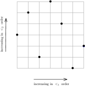
(a) the initial three elements induce the pattern 231.

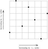
(b) contains 231 but not on the initial three elements.

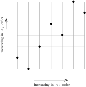
(c) does not contain 231.

Figure 1.1:

It is not hard to see that for a uniform random permutation the probability that $\pi(1)<\pi(2)$ equals $1/2$. So in particular, for uniform permutations $\operatorname{\mathsf{TOTO}}$ does not satisfy a zero-one law. See also the remark following Question 1 in [2]. What is more, in $\operatorname{\mathsf{TOTO}}$ uniform permutations do not even satisfy the convergence law as was first shown by Foy and Woods [24]. Let us also mention two very recent results on logical limit laws for random permutations. In [3] it is shown the uniform distribution on the set of permutations in $S_{n}$ that avoid 231 admits a convergence law in $\operatorname{\mathsf{TOTO}}$, and in [12] it is shown the same result holds for the uniform distribution on the class of layered permutations.

Both $\operatorname{\mathsf{TOOB}}$ and $\operatorname{\mathsf{TOTO}}$ fall under the umbrella of first order logical languages, as they only allow quantification over the elements of the domain. In contrast, second order logic also allows us to quantify over relations. Second order logic is much more powerful than first order logic. It is for instance possible to express in second order logic the property that the domain has an even number of elements. In particular, the convergence law will fail for second order logic, for trivial reasons.

The study of first order properties of random permutations is part of a larger theory of first order properties of random discrete structures. See for instance the monograph [60]. Examples of structures for which the first order properties have been studied include the Erdős-Rényi random graph (see e.g. [38],[60]), Galton-Watson trees [56], bounded degree graphs [42], random graphs from minor-closed classes [34], random perfect graphs [51], random regular graphs [31] and the very recent result on bounded degree uniform attachment graphs [49].

Let us also mention some work on random orders that is closely related to the topic of the present paper. The logic of random orders was introduced in [65] and has a single binary relation $<$. To sample a “$k$-dimensional” random order on $[n]$ pick $k$ random orderings $<_{1},\ldots,<_{k}$ on $[n]$ and set $x<y$ if $x<_{i}y$ in each of the orders $i=1,\ldots,k$. Notice that every sentence expressible with the single order $<$ in a two dimensional random order is expressible in $\operatorname{\mathsf{TOTO}}$; each of instance of $(x<y)$ we replace by $(x<_{1}y)\land(x<_{2}y)$. Non-convergence was proven for two dimensional random orders in [59] by constructing a first–order sentence $\varphi$ for which no limit probability exists; and this yields a constructive proof of non-convergence also in random permutations (adding to the earlier non-constructive proof [24]). Many properties of random orders are known [4, 10], see [14] and [15] for surveys of different models of random partial orders and also their relation to theories of spacetime [15].

An appeal of $\operatorname{\mathsf{TOTO}}$ is it allows one to express pattern containment (though not counting of patterns above a constant). Permutation patterns arise naturally in statistics. Let $(X,Y)$ be drawn from a continuous distribution on $\mathbb{R}^{2}$ and suppose we have $n$ random samples $(X_{i},Y_{i})$. Many statistical tests rely only on the relative ordering in the two dimensions, i.e. on the permutation induced by the $n$ points. For example the Kendall rank correlation coefficient is $\tau=1-2\operatorname{inv}(\pi)/\binom{n}{2}$ and indeed there is a test for independence of $X$ and $Y$ using only counts of permutations of length 4 [43, 66]. See [22] for a combinatorial account of the use of permutation patterns in statistics.

1.1 Main results

The main results of this paper are collected in the following two theorems:

Theorem 1.1.

In $\operatorname{\mathsf{TOOB}}$ the following holds:

1. [Compton,[16]] For $q=1$ the $\operatorname{Mallows}(n,q)$ distribution satisfies the convergence law but not the zero–one law;

2. If $q<1$ is fixed then $\operatorname{Mallows}(n,q)$ satisfies the zero–one law;

3. If $q>1$ is fixed then $\operatorname{Mallows}(n,q)$ does not satisfy the convergence law.

(Part (i) of Theorem 1.1 was already shown by Compton [16] in 1989, who in fact showed a much stronger statement.)

The function $\log^{*}n$ equals the number of times we need to iterate the base two logarithm to reach a number below one (starting from $n\in\mathbb{N}$).

Theorem 1.2.

In $\operatorname{\mathsf{TOTO}}$ the following holds:

1. If $q\neq 1$ is fixed, then the convergence law holds for $\operatorname{Mallows}(n,q)$ but not the zero–one law;

2. If $q=q(n)$ satisfies $1-\frac{1}{\log^{*}n}<q<1+\frac{1}{\log^{*}n}$, then the $\operatorname{Mallows}(n,q)$ distribution does not satisfy the convergence law.

Part (ii) of Theorem 1.2 extends a result of Foy and Woods [24] for uniform permutations (the case $q=1$).

The $\log^{*}n$ term is a very slowly growing function. As will be clear from the proof of Theorem 1.2 Part (ii), it is certainly not best possible and can be replaced by even more slowly growing functions, such as $\log^{**}n$ defined in Section 3.4, with little effort.

We will in fact show that there exists a single $\operatorname{\mathsf{TOTO}}$ formula $\varphi$ such that for all sequences $q=q(n)$ satisfying $1-\frac{1}{\log^{*}n}<q<1+\frac{1}{\log^{*}n}$, the quantity ${\mathbb{P}}\left(\Pi_{n}\models\varphi\right)$ does not have a limit as $n\to\infty$.

2 Overview of proof methods

Proof Sketch of Theorem 1.1: Theorem 1.1 concerns $\operatorname{\mathsf{TOOB}}$ and as such we consider the logic containing a single binary relation symbol $R$. The proof of Theorem 1.1 will rely on the following observations: Firstly, given any sentence $\varphi\in\operatorname{\mathsf{TOOB}}$ and $\pi\in S_{n}$ the vector of cycle counts $(C_{1}(\pi_{n}),\ldots,C_{n}(\pi_{n}))$ completely determines whether or not $\pi_{n}\models\varphi$ (where $C_{i}(\pi_{n})$ denotes the number of $i$–cycles in $\pi_{n}$). Secondly, it follows from the Hanf-Locality Theorem for bounded degree structures (Theorem 4.1) that for any fixed $\varphi\in\operatorname{\mathsf{TOOB}}$ there exists an $h\in{\mathbb{N}}$ such that for any $t\in{\mathbb{N}}$ and $n,m\geq h$, the sentence $\varphi$ cannot distinguish between the disjoint union of $n$ cycles of length $t$ and the disjoint union of $m$ cycles of length $t$. Moreover, this $h$ can be selected such that $\varphi$ additionally cannot distinguish between two cycles both of length at least $h$.

For $\Pi_{n}\sim\operatorname{Mallows}(n,q)$ with $0<q<1$, we use a result given in [33] by Jimmy He together with the first and last author of the current paper. They show that there are positive constants $m_{1},m_{2},\ldots$ depending on $q$ such that $\frac{1}{\sqrt{n}}\left(C_{1}(\Pi_{n})-m_{1}n,\ldots,C_{\ell}(\Pi_{n})-m_{\ell}n\right)$ converges in distribution to a multivariate normal with zero mean. This implies in particular that $\Pi_{n}$ will contain more than $h$ cycles of each of the lengths $1,\ldots,h$ giving the zero–one–law for $0<q<1$.

For fixed $q>1$, another result (Theorem 3.12) from [33] implies the existence of a vector $(c_{1},\ldots,c_{\ell})$ such that for $\Pi_{n}\sim\operatorname{Mallows}(n,q)$ the quantity ${\mathbb{P}}(C_{1}(\Pi_{n})=c_{1},\ldots,C_{\ell}(\Pi_{n})=c_{\ell})$ does not have a limit as $n\to\infty$. This property can be queried by a $\operatorname{\mathsf{TOOB}}$ sentence, establishing that $\operatorname{Mallows}(n,q)$ does not satisfy the convergence law w.r.t. $\operatorname{\mathsf{TOOB}}$ for fixed $q>1$.

Proof Sketch of Theorem 1.2 Part (i): The proof of Theorem 1.2 Part (i) is inspired by the approach taken by Lynch in [46] to show a convergence law for random strings having certain letter distributions. We consider some $\operatorname{\mathsf{TOTO}}$ sentence $\varphi$ having quantifier depth $d$. Writing $\pi\equiv_{d}\sigma$ if $\pi$ and $\sigma$ agree on all $\operatorname{\mathsf{TOTO}}$ sentences of depth at most $d$, we note that $\equiv_{d}$ is an equivalence relation with only finitely many equivalence classes (Theorem 3.20). We now rely on a sampling procedure for $\operatorname{Mallows}(n,q)$ distributed permutations. The details of the construction will be given in Section 3.2.2, it suffices to know that from a sequence $Z_{1},Z_{2},\ldots Z_{n}$ of independent $\operatorname{Geo}(1-q)$ random variables we may construct $\Pi_{n}$ by first determining the image of $1$ under $\Pi_{n}$ using $Z_{1}$, then the image of $2$ using $Z_{1},Z_{2}$ and so on. Taking a dynamic viewpoint, we can imagine exposing the values $Z_{1},Z_{2},\ldots$ one by one and following the sequence of permutations that arises. Foregoing complicating details, we can define in this manner a Markov chain on a countably infinite state space that follows the equivalence class under $\equiv_{d}$ of this sequence of permutations. We show that we can divide the state space into finitely many classes, each them irreducible aperiodic and positive recurrent, and that the chain will hit such a class a.a.s. Then standard results on the convergence of Markov chains will give the convergence of the quantify ${\mathbb{P}}(\Pi_{n}\models\varphi)$ as $n\to\infty$.

Proof Sketch of Theorem 1.2 Part (ii): The proof of Theorem 1.2 Part (ii) proceeds in several steps. First we determine a sentence $\varphi$ such that for $\Pi_{n}\sim\operatorname{Mallows}(n,1)$ we have

$${\mathbb{P}}(\Pi_{n}\models\varphi)=\begin{cases}1-O(n^{-100})&\text{if }\log^{**}\log^{**}n\text{ is even},\\ O(n^{-100})&\text{if }\log^{**}\log^{**}n\text{ is odd}.\end{cases}$$ (2)

for infinitely many $n$. We need some additional technical conditions on the values of $n$ such that the above is satisfied but we do not mention them here. We note that this is an explicit version of a result by Foy and Woods given in [24] (and which differs from the construction by Spencer in [59]). We show this result by associating pairs of intervals in $\Pi_{n}\sim\operatorname{Mallows}(n,1)$ to directed graph structures having $N=\Theta(\log\log n)$ vertices. See Figure 6.2 for an example permutation and pair of intervals corresponding to a directed cherry. The directed graph corresponding to the permutation is random, and the number of pairs of intervals is sufficiently high so that with high probability we will be likely to find any directed graph on $N$ vertices. We then adapt the method developed by Spencer and Shelah in [58] of using graphs to model arithmetic on sets to find a sentence about these graphs that oscillates between being true and false depending on $N$, which will provide the dependency of ${\mathbb{P}}\left(\Pi_{n}\models\varphi\right)$ on the parity of $\log^{**}\log^{**}n$.

We then show that if $q=1-O(n^{-4})$ then the total variation distance between $\operatorname{Mallows}(n,q)$ and $\operatorname{Mallows}(n,1)$ is $O(n^{-2})$. This allows us to extend the previous result from $q=1$ to $q=1-O(n^{-4})$, replacing the $O(n^{-100})$ terms in (2) by $O(n^{-2})$. We extend the result twice more but now we will have to work a little harder each time.

If $j\in[n]$ and $\Pi_{n}\sim\operatorname{Mallows}(n,q)$ then $\Pi_{j}$, the permutation of $[j]$ inheriting the order of $\Pi_{n}|_{[j]}$ follows a $\operatorname{Mallows}(j,q)$ distribution. We consider now $q=1-O(1/n)$ and define $J_{1}(\pi)$ as the smallest $j\in[n]$ for which there exists an $i\in[j]$ satisfying $\pi(i)+1\in\pi[[j]]$. For a uniform permutation $\Pi^{*}_{n}\in S_{n}$ we have ${\mathbb{E}}|\{i:\{\Pi_{n}(i),\Pi_{n}(i)+1\}\subseteq\Pi_{n}[[j]]\}|\approx j\cdot j/n$, and it turns out the $q=1-O(1/n)$ case is close enough to the uniform case that we will have $J_{1}(\Pi_{n})=\Theta(\sqrt{n})$. Then we define $K_{1}(\Pi_{n})\coloneqq J_{1}(\Pi_{J_{1}(\Pi_{n})})$ where $K_{1}(\Pi_{n})=\Theta(n^{1/4})$ will be shown to hold with probability $1-\varepsilon$ for some $\varepsilon>0$. See Figure 7.1. Now $\Pi_{K_{1}(\Pi_{n})}$ is roughly distributed as $\operatorname{Mallows}(\Theta(n^{1/4}),q)$ with $q=1-O(1/n)=1-O(K_{1}^{-4})$, where we must take care of some dependency between $K_{1}$ and the induced permutation $\Pi_{n}|_{K_{1}(\Pi_{n})}$. We then apply the previous result to show non–convergence for the case $q=1-O(1/n)$.

We subsequently extend the result once more, where we now set $N=\Pi^{-1}_{n}(1)+1$. By a result of Bhatnagar and Peled [9] (Theorem 3.15) we will have $N=\Theta(1/(1-q))$ so that also $q=1-\Theta(1/N)$. Moreover, we show that $\Pi_{N-1}$ follows a $\operatorname{Mallows}(N-1,q)$ distribution. Here we will additionally have to handle the case $q>1$ and $q<1$ separately at first. However, defining the sentence $\rho$ saying that $\Pi_{n}(1)>\Pi_{n}(n)$ provides us with a mechanism to ’detect’ when $q>1$, in which case $\rho$ will likely be satisfied, and when $q<1$ in which case $\rho$ is likely not satisfied. This allows us to give a single (universal) non–convergent sentence $\varphi$ such that ${\mathbb{P}}\left(\Pi_{n}\models\varphi\right)$ does not convergence for $\Pi_{n}\sim\operatorname{Mallows}(n,q)$ for all $1-1/\log^{*}n<q<1+1/\log^{*}n$.

3 Notation and preliminaries

We use the notation ${\mathbb{N}}=\{1,2,\ldots\}$ and ${\mathbb{Z}}_{\geq 0}=\{0,1,\ldots\}$.

3.1 Requisites from probability theory

We collect here some mostly well–known results from probability theory.

Theorem 3.1 (Chernoff’s inequality).

Let $X_{1},\ldots,X_{n}$ be independent such that $0\leq X_{i}\leq 1$ for $i\in[n]$. Define $S_{n}\coloneqq X_{1}+\ldots+X_{n}$ and $\mu\coloneqq{\mathbb{E}}S_{n}$. Let $0<\varepsilon<1$, then

$${\mathbb{P}}\left(S_{n}\geq(1+\varepsilon)\mu\right)\leq\exp\left\{-\frac{\mu\varepsilon^{2}}{3}\right\},$$ (3)

$${\mathbb{P}}\left(S_{n}\leq(1-\varepsilon)\mu\right)\leq\exp\left\{-\frac{\mu\varepsilon^{2}}{2}\right\}.$$ (4)

Panconesi and Srinivasan in [53] developed a generalization of Chernoff’s bound that omits the condition that the $X_{i}$ be independent.

Theorem 3.2.

Let $X_{1},\ldots,X_{n}$ be random variables taking values in $\{0,1\}$ such that, for some $0\leq\delta\leq 1$, we have that, for every subset $S\subseteq[n]$, ${\mathbb{P}}\left(\bigwedge_{i\in S}X_{i}=1\right)\leq\delta^{|S|}$. Then, for any $0\leq\delta\leq\gamma\leq 1$

$${\mathbb{P}}\left(\sum_{i=1}^{n}X_{i}\geq\gamma n\right)\leq e^{-2n(\gamma-\delta)^{2}}.$$ (5)

We denote by $\operatorname{Bi}(n,p)$ the binomial distribution. We will need the following crude bound:

Lemma 3.3.

Let $X\sim\operatorname{Bi}(n,k/n)$ for $0\leq k\leq n$. Then ${\mathbb{P}}\left(X=k\right)\geq 1/(n+1)$.

Proof.

If $k=n$ then the result is clear, so assume that $k\neq n$. Setting $p=n/k$ we have for all $1\leq j\leq n$ that

$$\frac{{\mathbb{P}}\left(X=j\right)}{{\mathbb{P}}\left(X=j-1\right)} =\frac{\binom{n}{j}(1-p)^{n-j}p^{j}}{\binom{n}{j-1}(1-p)^{n-j+1}p^{j-1}}=\frac{(n-j+1)p}{j(1-p)}.$$ (6)

The right–hand side above is less than one if and only if

$$j-jp>(n-j+1)p\quad\iff\quad j>\frac{(n+1)k}{n}\quad\iff\quad j\geq k+1,$$ (7)

the last equivalence holding due to $j$ being an integer and $k\neq n$. Thus ${\mathbb{P}}\left(X=j\right)$ is maximized at $j=k$. As there are only $n+1$ possible outcomes for $X$ we therefore must have ${\mathbb{P}}\left(X=k\right)\geq 1/(n+1)$. ∎

Given two discrete probability distributions $\mu_{1}$ and $\mu_{2}$ on a countable set $\Omega$, their total variation distance is defined as

$$d_{\operatorname{TV}}(\mu_{1},\mu_{2})=\max_{A\subseteq\Omega}|\mu_{1}(A)-\mu_{2}(A)|.$$ (8)

This can be expressed alternatively as

$$d_{\operatorname{TV}}(\mu_{1},\mu_{2})=\frac{1}{2}\sum_{x\in\Omega}|\mu_{1}(x)-\mu_{2}(x)|=\sum_{x:\mu_{1}(x)>\mu_{2}(x)}\mu_{1}(x)-\mu_{2}(x).$$ (9)

(See for instance Proposition 4.2 in [44] for a proof.) As is common, we will interchangeably use the notation $d_{\operatorname{TV}}(X,Y):=d_{\operatorname{TV}}(\mu,\nu)$ if $X\sim\mu$ and $Y\sim\nu$.

A coupling of two probability measures $\mu,\nu$ is a joint probability measure for a pair of random variables $(X,Y)$ satisfying $X\hskip 0.86108pt\raisebox{-0.43057pt}{$=$}\raisebox{4.30554pt}{{$\scriptstyle d$}}\hskip 3.44444pt\mu,Y\hskip 0.86108pt\raisebox{-0.43057pt}{$=$}\raisebox{4.30554pt}{{$\scriptstyle d$}}\hskip 3.44444pt\nu$. We will also speak of a coupling of $X,Y$ as being a probability space for $(X^{\prime},Y^{\prime})$ with $X^{\prime}\hskip 0.86108pt\raisebox{-0.43057pt}{$=$}\raisebox{4.30554pt}{{$\scriptstyle d$}}\hskip 3.44444ptX,Y^{\prime}\hskip 0.86108pt\raisebox{-0.43057pt}{$=$}\raisebox{4.30554pt}{{$\scriptstyle d$}}\hskip 3.44444ptY$.

Lemma 3.4.

Let $\mu$ and $\nu$ be two probability distributions on the same countable set $\Omega$. Then

$$d_{\operatorname{TV}}(\mu,\nu)=\inf\{{\mathbb{P}}\left(X\neq Y\right):(X,Y)\text{ is a coupling of $\mu$ and $\nu$}\}.$$ (10)

There is a coupling that attains this infimum.

(See for instance [44], Proposition 4.7 and Remark 4.8 for a proof.)

For $n\in{\mathbb{N}}$ and $p\in(-\infty,0)\cup(0,1)$ we define the $\operatorname{TruncGeo}(n,p)$ distribution where $Y\sim\operatorname{TruncGeo}(n,p)$ means

$${\mathbb{P}}(Y=k)=\frac{p(1-p)^{k-1}}{1-(1-p)^{n}},\qquad k\in\{0,\ldots,n\}.$$ (11)

Observe that if $p\in(0,1)$ then, setting $X\sim\operatorname{Geo}(p)$, the probability mass in (11) is exactly equal to ${\mathbb{P}}\left(X=k\,|\,X\leq n\right)$. Therefore we shall refer to the $\operatorname{TruncGeo}(n,p)$ as the truncated geometric distribution. But we stress that the $\operatorname{TruncGeo}(n,p)$ is a valid probability distribution for any $p\in(-\infty,0)\cup(0,1)$.

3.1.1 Markov chains

We give here a brief overview of some of the concepts related to Markov chains which will be used in Section 5. The following definitions and results are widely known and can be found in most books on Markov chains or more general stochastic processes, see for instance [44], [30] or [52].

Let $X_{n}$ be a Markov chain with state space ${\mathcal{S}}$. Given $i,j\in{\mathcal{S}}$, if ${\mathbb{P}}\left(X_{n}=j\,|\,X_{0}=i\right)>0$ for some $n\in{\mathbb{Z}}_{\geq 0}$ we say that $j$ is reachable from $i$. We denote this also by $i\to j$. If $i\to j$ and $j\to i$ then we say that the states $i$ and $j$ communicate and we write $i\leftrightarrow j$. The relation $\leftrightarrow$ is an equivalence relation, the equivalence classes under $\leftrightarrow$ will be called communicating classes. For every state $i\in{\mathcal{S}}$ we have $i\leftrightarrow i$. In the case that the entire state space is a single communicating class we call the Markov chain irreducible. The evolution of a Markov chain depends on the initial distribution over the states. If $X_{0}=i$ for some $i\in{\mathcal{S}}$ then we write ${\mathbb{P}}_{i}(\cdot)$ for the corresponding probability and ${\mathbb{E}}_{i}(\cdot)$ for the expectation. If $X_{0}$ is distributed according to some distribution $\mu_{0}$ over ${\mathcal{S}}$ then we write ${\mathbb{P}}_{\mu_{0}}$ and ${\mathbb{E}}_{\mu_{0}}$.

For any $i\in{\mathcal{S}}$ we define $\tau_{i}$ to be the first time that the Markov chain is in state $i$, and we define $\tau^{+}_{i}>0$ to be the first time after zero that the Markov chain is in state $i$, given that $X_{0}=i$. If ${\mathbb{P}}_{i}(\tau^{+}_{i}<\infty)=1$ then we say that the state $i$ is recurrent, otherwise we say that it is transient. If additionally ${\mathbb{E}}_{i}\tau^{+}_{i}<\infty$ then we say that $i$ is positive recurrent. If ${\mathcal{S}}$ is finite then recurrence implies positive recurrence. If $i$ is transient, then all $j$ in the communicating class containing $i$ are transient, and similarly if $i$ is (positive) recurrent. Thus we will talk about positive recurrent classes etc. If $X_{n}$ is in a recurrent class for some $n$, then $X_{n+k}$ is contained in this class for all $k\geq 0$.

Proofs for the following two results are given in Theorem 4 and Lemma 5, respectively, in Section 6.3 of [30].

Theorem 3.5.

The state space ${\mathcal{S}}$ of a Markov chain can be partitioned uniquely as

$${\mathcal{S}}=T\cup C_{1}\cup C_{2}\cup\ldots$$ (12)

where $T$ is the set of transient states, and the $C_{i}$ are irreducible closed sets of of recurrent states.

Lemma 3.6.

If ${\mathcal{S}}$ is finite, then at least one state is recurrent and all recurrent states are positive recurrent.

Lemma 3.7.

If ${\mathcal{S}}$ is finite then with probability $1$ the chain $X_{n}$ will be in a recurrent state for some $n\geq 0$.

Proof.

Let ${\mathcal{S}}=T\cup C_{1}\cup C_{2}\cup\ldots$ be as in Theorem 3.5. For each of the finitely many $i\in T$ there is a positive probability that the chain moves from $i$ to a state in ${\mathcal{S}}\setminus T$ in at most $|T|$ steps. Then ${\mathbb{P}}\left(X_{n}\in T\right)\leq Kc^{n}$ for some constants $K>0$ and $0<c<1$. By the Borel–Cantelli Lemma, $X_{n}$ is in $T$ for only finitely many $n$, so that it must visit a recurrent state. ∎

The following theorem is the Markov chain convergence theorem, see e.g. [20] Theorem 7.6.4 for a proof (note that in [20], what we call irreducibility is called strong irreducibility).

Theorem 3.8 (Markov chain convergence theorem).

Let $P$ be a Markov kernel on a discrete (countable) state space ${\mathcal{S}}$. Assume that $P$ is irreducible, aperiodic and positive recurrent. There exists a unique invariant probability measure $\pi$ over ${\mathcal{S}}$ such that for every probability measure $\mu_{0}$ over ${\mathcal{S}}$

$$\lim_{n\to\infty}d_{\operatorname{TV}}(\mu_{0}P^{n},\pi)=0.$$ (13)

The following result is alluded to in many texts on Markov chains when discussing the convergence behavior of a Markov chains that are not irreducible. We have not found an appropriate reference however so we state and prove here a result that we will need in Section 5.

Lemma 3.9.

Let $X_{n}$ be a Markov chain on the countable state space ${\mathcal{S}}$, and let ${\mathcal{M}}$ be a communicating class of $X_{n}$ such that the chain restricted to ${\mathcal{M}}$ is aperiodic, irreducible and positive recurrent. Then the limit

$$\lim_{n\to\infty}{\mathbb{P}}\left(X_{n}\in A\,|\,\tau_{{\mathcal{M}}}<\infty\right)$$ (14)

exists for all $A\subseteq{\mathcal{M}}$.

Proof.

We have

$${\mathbb{P}}\left(X_{n}\in A\,|\,\tau_{{\mathcal{M}}}<\infty\right)=\sum\limits_{j=0}^{\infty}{\mathbb{P}}\left(X_{n}\in A\,|\,\tau_{{\mathcal{M}}}=j\right){\mathbb{P}}\left(\tau_{{\mathcal{M}}}=j\,|\,\tau_{{\mathcal{M}}}<\infty\right).$$ (15)

Conditioning on $\tau_{{\mathcal{M}}}=j$ induces a probability distribution $\nu_{j}$ over the states in ${\mathcal{M}}$ where for $B\subseteq{\mathcal{M}}$ we have $\nu_{j}(B)={\mathbb{P}}\left(X_{j}\in B\,|\,\tau_{{\mathcal{M}}}=j\right)$. The Markov chain $X_{n}$ restricted to ${\mathcal{M}}$ is assumed aperiodic, irreducible and positive recurrent. So by Theorem 3.8 there exits a unique distribution $\pi$ over ${\mathcal{M}}$ such that for all $j\in{\mathbb{Z}}_{\geq 0}$

$$\lim_{n\to\infty}{\mathbb{P}}\left(X_{n}\in A\,|\,\tau_{{\mathcal{M}}}=j\right)=\lim_{n\to\infty}{\mathbb{P}}_{\nu_{j}}\left(X_{n-j}\in A\right)=\pi(A).$$ (16)

Now, let $\varepsilon>0$ be arbitrary, and let $j_{0}\in{\mathbb{Z}}_{\geq 0}$ be such that ${\mathbb{P}}\left(\tau_{{\mathcal{M}}}>j_{0}\,|\,\tau_{{\mathcal{M}}}<\infty\right)<\varepsilon/2$. Then

$$\left|{\mathbb{P}}\left(X_{n}\in A\,|\,\tau_{{\mathcal{M}}}<\infty\right)-\pi(A)\right|\ \ \leq\ \ \sum\limits_{j=0}^{\infty}\left|{\mathbb{P}}\left(X_{n}\in A\,|\,\tau_{{\mathcal{M}}}=j\right)-\pi(A)\right|{\mathbb{P}}\left(\tau_{{\mathcal{M}}}=j\,|\,\tau_{{\mathcal{M}}}<\infty\right)$$ (17)

$$<\ \ \left(1-\frac{\varepsilon}{2}\right)\max\limits_{0\leq j\leq j_{0}}\left|{\mathbb{P}}\left(X_{n}\in A\,|\,\tau_{{\mathcal{M}}}=j\right)-\pi(A)\right|+\frac{\varepsilon}{2}$$ (18)

The maximum above is taken over a finite set, so by (16) there exists an $n_{0}$ such that $n\geq n_{0}$ implies that the above is at most $\varepsilon$. Thus,

$$\lim_{n\to\infty}{\mathbb{P}}\left(X_{n}\in A\,|\,\tau_{{\mathcal{M}}}<\infty\right)=\pi(A).$$ (19)

∎

3.2 Mallows permutations

It is a standard result in enumerative combinatorics (see Corollary 1.3.13 in [61]) that for $q\neq 1$ the denominator in the definition of the Mallows distribution (1) satisfies

$$\sum_{\sigma\in S_{n}}q^{\operatorname{inv}(\sigma)}=\prod_{i=1}^{n}\frac{1-q^{i}}{1-q}.$$ (20)

We define for $n\geq 1$ the permutation $r_{n}:i\mapsto n-i+1$. For every $\pi\in S_{n}$ we have

$$\operatorname{inv}(r_{n}\circ\pi) =\operatorname{inv}(\pi\circ r_{n})=\binom{n}{2}-\operatorname{inv}(\pi),$$ (21)

$$\operatorname{inv}(\pi^{-1}) =\operatorname{inv}(\pi).$$ (22)

That is, if $\Pi_{n}\sim\operatorname{Mallows}(n,q)$, then $r_{n}\circ\Pi_{n}\hskip 0.86108pt\raisebox{-0.43057pt}{$=$}\raisebox{4.30554pt}{{$\scriptstyle d$}}\hskip 3.44444pt\Pi_{n}\circ r_{n}\hskip 0.86108pt\raisebox{-0.43057pt}{$=$}\raisebox{4.30554pt}{{$\scriptstyle d$}}\hskip 3.44444pt\operatorname{Mallows}(n,1/q)$ and $\Pi^{-1}_{n}\hskip 0.86108pt\raisebox{-0.43057pt}{$=$}\raisebox{4.30554pt}{{$\scriptstyle d$}}\hskip 3.44444pt\operatorname{Mallows}(n,q)$.

For $X=\{x_{1},\dots,x_{n}\}$ a set of distinct numbers and $x\in X$ we define the rank $\operatorname{rk}(x,X)$ of $x$ in $X$ as the unique $i$ such that $x$ is the $i$-th smallest element of $X$. For $x=(x_{1},\dots,x_{n})$ a sequence of distinct numbers, let us write

$$\operatorname{rk}(x_{1},\dots,x_{n}):=\left(\operatorname{rk}(x_{1},\{x_{1},\dots,x_{n}\}),\dots,\operatorname{rk}(x_{n},\{x_{1},\dots,x_{n}\})\right).$$ (23)

With some abuse of notation we will sometimes write $\pi=\operatorname{rk}(x_{1},\ldots,x_{n})$ to mean that $\pi\in S_{n}$ is the permutation satisfying $\pi(i)=\operatorname{rk}(x_{i},\{x_{1},\ldots,x_{n}\})$ for all $i\in[n]$.

Lemma 3.10 ([9], Corollary 2.7).

Let $(i,i+1,\ldots,i+m-1)\in[n]$ be a sequence of consecutive elements. If $\Pi_{n}\sim\operatorname{Mallows}(n,q)$

$$\operatorname{rk}(\Pi_{n}(i),\ldots,\Pi_{n}(i+m-1))\hskip 0.86108pt\raisebox{-0.43057pt}{$=$}\raisebox{4.30554pt}{{$\scriptstyle d$}}\hskip 3.44444pt\operatorname{Mallows}(m,q).$$ (24)

In [27] Gnedin and Olshansky introduced a random bijection $\Sigma:{\mathbb{Z}}\to{\mathbb{Z}}$ which is a natural extension to the finite $\operatorname{Mallows}(n,q)$ model with $0<q<1$. We denote this distribution by $\operatorname{Mallows}({\mathbb{Z}},q)$ where $0<q<1$. We will not need the details of the construction and refer the reader to the original paper for a detailed description.

In [33], Jimmy He together with the first and last author of the current paper studied the limit behavior of the cycles counts of $\operatorname{Mallows}(n,q)$ distributed random permutations for fixed $q\neq 1$. Given a permutation $\pi\in S_{n}$ we define $C_{i}(\pi)$ to be the number of $i$–cycles of $\pi$ for $i\geq 1$. We will use the following results:

Theorem 3.11 ([33], Theorem 1.1).

Fix $0<q<1$ and let $\Pi_{n}\sim\operatorname{Mallows}(n,q)$. There exist positive constants $m_{1},m_{2},\ldots$ and an infinite matrix $P\in{\mathbb{R}}^{{\mathbb{N}}\times{\mathbb{N}}}$ such that for all $\ell\geq 1$ we have

$$\frac{1}{\sqrt{n}}\left(C_{1}(\Pi_{n})-m_{1}n,\ldots,C_{\ell}(\Pi_{n})-m_{\ell}n\right)\quad\xrightarrow[n\to\infty]{d}\quad{\mathcal{N}}_{\ell}(\underline{0},P_{\ell}),$$ (25)

where ${\mathcal{N}}_{\ell}(\cdot,\cdot)$ denotes the $\ell$–dimensional multivariate normal distribution and $P_{\ell}$ is the submatrix of $P$ on the indices $[\ell]\times[\ell]$.

We define the bijections $r,\rho:{\mathbb{Z}}\to{\mathbb{Z}}$ by $r(i)=-i$ and $\rho(i)=1-i$.

Theorem 3.12 ([33], Theorem 1.3).

Let $q>1$ and $\Pi_{n}\sim\operatorname{Mallows}(n,q)$ and $\Sigma\sim\operatorname{Mallows}({\mathbb{Z}},1/q)$. We have

$$(C_{1}(\Pi_{2n+1}),C_{3}(\Pi_{2n+1}),\ldots)\xrightarrow[n\to\infty]{d}\quad(C_{1}(r\circ\Sigma),C_{3}(r\circ\Sigma),\ldots)$$

and

$$(C_{1}(\Pi_{2n}),C_{3}(\Pi_{2n}),\ldots)\xrightarrow[n\to\infty]{d}\quad(C_{1}(\rho\circ\Sigma),C_{3}(\rho\circ\Sigma),\ldots).$$

Moreover, the two limit distributions above are distinct for all $q>1$.

Remark 3.13.

The convergence in Theorem 3.12 should be understood to mean that for all sequences $c_{1},c_{3},\ldots$ with only finitely many nonzero values we have

$${\mathbb{P}}\left((C_{1}(\Pi_{2n+1}),C_{3}(\Pi_{2n+1}),\ldots)=(c_{1},c_{3},\ldots)\right)\ \xrightarrow[n\to\infty]{\,}\,\,\,{\mathbb{P}}\left((C_{1}(r\circ\Sigma),C_{3}(r\circ\Sigma),\ldots)=(c_{1},c_{3},\ldots)\right).$$ (26)

For sequences $c_{1},c_{3},\ldots$ with infinitely many nonzero values the limit of the left hand side above is zero, as is the limit of the right–hand side.

When $q=1$ the Mallows distribution simply samples a permutation of $1,\dots,n$ uniformly at random. A classical result going back to Gontcharoff [28] and Kolchin [41] states that in this case, for every fixed $\ell$:

$$\left(C_{1}(\Pi_{n}),\dots,C_{\ell}(\Pi_{n})\right)\xrightarrow[n\to\infty]{\text{d}}\left(X_{1},\dots,X_{\ell}\right),$$

where $X_{1},\ldots,X_{\ell}$ are independent random variables with $X_{i}\sim\operatorname{Po}(1/i)$.

Arratia and Tavaré extend this result to convergence of the vector $(C_{1}(\Pi_{n}),\ldots,C_{b}(\Pi_{n}))$ in the case that $b=b(n)$ is such that $b/n\to 0$.

Theorem 3.14 ([6], Theorem 2).

Let $\Pi_{n}$ be selected uniformly from $S_{n}$, and let $X_{1},\ldots,X_{n}$ be a sequence of independent random variables where $X_{i}\sim\operatorname{Po}(1/i)$ for $i=1,\ldots,n$. Let $b=b(n):{\mathbb{N}}\to{\mathbb{N}}$ be a function. Then

$$d_{\operatorname{TV}}((C_{1}(\Pi_{n}),\ldots,C_{b}(\Pi_{n})),(X_{1},\ldots,X_{b}))\ \xrightarrow[n\to\infty]{\,}\,0$$ (27)

if and only if $b/n\to 0$.

The following result is due to Bhatnagar and Peled.

Theorem 3.15 ([9], Theorem 1.1).

For all $0<q<1$, and integer $1\leq i\leq n$, if $\Pi_{n}\sim\operatorname{Mallows}(n,q)$ then

$${\mathbb{E}}|\Pi_{n}(i)-i|\leq\min\left(\frac{2q}{1-q},n-1\right).$$ (28)

3.2.1 Construction using truncated geometric random variables

The following method of sampling a $\operatorname{Mallows}(n,q)$ distributed permutation for $q<1$ goes back to the work of Mallows [48]. Let $Z_{1},\dots,Z_{n}$ be independent with $Z_{i}\sim\allowbreak{\operatorname{TruncGeo}(n-i+1,1-q)}$. We now set

$$\Pi_{n}(1) =Z_{1},$$ (29)

$$\Pi_{n}(i) =\text{the $Z_{i}$-th smallest number in the set }[n]\setminus\{\Pi_{n}(1),\ldots,\Pi_{n}(i-1)\},\qquad\text{ for $1<i\leq n$}.$$ (30)

Then $\Pi_{n}$ follows a $\operatorname{Mallows}(n,q)$ distribution. If in this construction we replace the $Z_{i}$ with independent uniform random variables on the the set $[n-i+1]$, then the above procedure samples a uniformly distributed permutation from $S_{n}$.

3.2.2 Construction using geometric random variables

In [55] Pitman and Tang give a general construction for a random bijection $\Pi:{\mathbb{N}}\to{\mathbb{N}}$: For a probability distribution $p$ on ${\mathbb{N}}$ with $p(1)>0$ they call a random permutation $\Pi$ of ${\mathbb{N}}$ a $p$–shifted random permutation of ${\mathbb{N}}$ if for $Z_{1},Z_{2},\ldots$ i.i.d. sampled according to $p$, we set

$$\Pi(1) \coloneqq Z_{1}$$ (31)

$$\Pi(i) \coloneqq\text{the $Z_{i}$-th smallest element in the set $\mathbb{N}\setminus\{\Pi(1),\dots,\Pi(i-1)\}$},\qquad\text{for }i>1.$$ (32)

Proposition 3.16 ([55], Proposition 1.4(v)).

For each fixed probability distribution $p$ on ${\mathbb{N}}$ with $p(1)>0$, and $\Pi$ a $p$–shifted random permutation of ${\mathbb{N}}$, if $\sum_{i}ip(i)<\infty$ then $\Pi$ is positive recurrent.

Here a random permutation is defined to be positive recurrent if with probability $1$ there are infinitely many $T\in{\mathbb{N}}$ such that $\Pi[[T]]=[T]$. Such $T$ are called regeneration times, they will be examined in more detail in Section 5.

If $p$ is a $\operatorname{Geo}(1-q)$ distribution we denote the distribution of a $p$–shifted random permutation of ${\mathbb{N}}$ by $\operatorname{Mallows}({\mathbb{N}},q)$. The $\operatorname{Mallows}({\mathbb{N}},q)$ distribution was first studied by Gnedin and Olshanki in [26].

Remark 3.17.

To any $\pi\in S_{n}$ we can uniquely associate a sequence $z_{1},\ldots,z_{n}$ such that if $\Pi\sim\operatorname{Mallows}({\mathbb{N}},q)$ is constructed from an i.i.d. sequence $Z_{1},Z_{2},\ldots$ of $\operatorname{Geo}(1-q)$ random variables as described, then $\{\Pi\upharpoonright[n]=\pi\}=\{Z_{1}=z_{1},\ldots,Z_{n}=z_{n}\}$. In particular, for any $\pi\in S_{n}$ we have ${\mathbb{P}}(\Pi\upharpoonright[n]=\pi)>0$.

The following result was obtained by Basu and Bhatnagar ([7], Lemma 2.1) and independently by Crane and DeSalvo ([17], Lemma 5.2):

Lemma 3.18.

For $q<1$, if $\Pi\sim\operatorname{Mallows}({\mathbb{N}},q)$ and $\Pi_{n}\coloneqq\operatorname{rk}(\Pi(1),\ldots,\Pi(n))$ then $\Pi_{n}\hskip 0.86108pt\raisebox{-0.43057pt}{$=$}\raisebox{4.30554pt}{{$\scriptstyle d$}}\hskip 3.44444pt\allowbreak\operatorname{Mallows}(n,q)$.

3.3 First–order logic

Given a set of relation symbols $R_{1},\ldots,R_{k}$ with associated arities $a_{1},\ldots,a_{k}$, we define ${\mathcal{L}}_{R_{1},\ldots,R_{k}}$ as the first–order language consisting of all first–order formulas built from the usual first–order connectives together with $R_{1},\ldots,R_{k}$. As an example, for a single binary relation $R$, we may consider the formula $\varphi_{0}(x)\in{\mathcal{L}}_{R}$ defined as

$$\varphi_{0}(x)\coloneqq R(x,x)\wedge\neg\exists y:(\neg(x=y)\wedge R(y,y)).$$ (33)

A free variable of a formula $\varphi$ is a variable that occurs outside of the scope of a quantifier. We write $\mathsf{Free}(\varphi)$ for the set of free variables in $\varphi$, and say that a formula with no free variables is a sentence. For $\varphi_{0}$ as in (33) we have $\mathsf{Free}(\varphi_{0})=\{x\}$. Given $R_{1},\ldots,R_{k}$ with arities $a_{1},\ldots,a_{k}$, a $(R_{1},\ldots,R_{k})$–structure ${\mathfrak{A}}$ is a tuple $(A,R_{1}^{\mathfrak{A}},\ldots,R_{k}^{\mathfrak{A}})$ where $A$ is a set, called the domain of ${\mathfrak{A}}$, and each $R_{j}^{{\mathfrak{A}}}$ is a relation of arity $a_{j}$ over $A$. We will routinely write simply $R_{j}$ for $R_{j}^{\mathfrak{A}}$ and talk about structures instead of $(R_{1},\ldots,R_{k})$–structures. If a structure ${\mathfrak{A}}$ satisfies a sentence $\varphi$ then we write ${\mathfrak{A}}\models\varphi$. Similarly, if $i_{1},\ldots,i_{k}$ are elements in the domain of ${\mathfrak{A}}$ and $\varphi(x_{1},\ldots,x_{k})$ is a formula with $\mathsf{Free}(\varphi)=\{x_{1},\ldots,x_{k}\}$ then we write $({\mathfrak{A}},i_{1},\ldots,i_{k})\models\varphi$ if $\varphi$ is satisfied by ${\mathfrak{A}}$ under the assignment $x_{j}\mapsto i_{j}$. We have for instance that $({\mathfrak{A}},i)\models\varphi_{0}$ precisely when the element $x$ is the unique element satisfying $R(x,x)$ in ${\mathfrak{A}}$.

For a complete and rigorous definition of formulas, free variables and structures satisfying formulas, see for instance Chapter 1 of [37].

Two $(R_{1},\ldots,R_{k})$–structures ${\mathfrak{A}},{\mathfrak{B}}$ with domain $A$ and $B$ respectively are called isomorphic if there is a bijection $f:A\to B$ such that

$$(i_{1},\ldots,i_{k})\in R_{j}^{{\mathfrak{A}}}\iff(f(i_{1}),\ldots,f(i_{k}))\in R_{j}^{{\mathfrak{B}}}\qquad\text{ for all $i_{1},\ldots,i_{k}\in A$ and all $R_{j}$.}$$ (34)

The following is a well–known result on isomorphic structures, see e.g. Theorem 3.4 of [57] for a proof.

Lemma 3.19.

If ${\mathfrak{A}}$ and ${\mathfrak{B}}$ are isomorphic, then for all sentences $\varphi$ we have ${\mathfrak{A}}\models\varphi$ if and only if ${\mathfrak{B}}\models\varphi$.

We recursively define the quantifier depth of a first–order sentence $\varphi$, denoted $D(\varphi)$, as follows:

• For any atomic formula $\varphi$ we set $D(\varphi)=0$;

• For any formula $\varphi$ we set $D(\neg\varphi)=D(\varphi)$;

• For any two formulas $\varphi,\psi$ we set $D(\varphi\wedge\psi)=D(\varphi\vee\psi)=\max\{D(\varphi),D(\psi)\}$;

• For a formula $\psi$ with at least one free variable we set $D(\exists x(\psi))=D(\forall x(\psi))=D(\psi(x))+1$.

If two structures ${\mathfrak{A}}$ and ${\mathfrak{B}}$ agree on all sentences $\varphi$ with $D(\varphi)\leq d$ we write ${\mathfrak{A}}\equiv_{d}{\mathfrak{B}}$ and say that ${\mathfrak{A}}$ and ${\mathfrak{B}}$ are $d$–equivalent. The relation $\equiv_{d}$ is an equivalence relation. The following lemma will be crucial in the proof of Theorem 5. A proof can be found for instance following Corollary 3.16 in [45].

Lemma 3.20.

The equivalence relation $\equiv_{d}$ has only finitely many equivalence classes.

Given two structures ${\mathfrak{A}},{\mathfrak{B}}$ with disjoint domains $A$ and $B$ we define ${\mathfrak{A}}\uplus{\mathfrak{B}}$ as the structure ${\mathfrak{C}}$ with domain $C=A\uplus B$ such that

$$R^{{\mathfrak{C}}}=R^{{\mathfrak{A}}}\uplus R^{{\mathfrak{B}}},\quad\text{ for all relation symbols $R$}.$$ (35)

In a more general setting where we allow also constants in our first–order language, we need to be careful with the above as we would have two conflicting candidates in ${\mathfrak{C}}$ for each constant. We will not have this problem as we do now use any constant symbols.

For a $(R_{1},\ldots,R_{k})$–structure ${\mathfrak{A}}$ we define $\operatorname{Th}({\mathfrak{A}})=\{\varphi\in{\mathcal{L}}_{R_{1},\ldots,R_{k}}:{\mathfrak{A}}\models\varphi\}$, often referred to as the complete theory of ${\mathfrak{A}}$. For $d\geq 0$ we define $\operatorname{Th}^{d}({\mathfrak{A}})$ as the set of all sentences $\varphi$ in $\operatorname{Th}({\mathfrak{A}})$ with quantifier depth at most $d$. The following theorem is due to Ehrenfeucht, Fraïssé, Feferman and Vaught, the statement as given is Theorem 1.5 in [47] which also includes a proof.

Theorem 3.21.

$\operatorname{Th}^{d}({\mathfrak{A}}\uplus{\mathfrak{B}})$ is uniquely determined by $\operatorname{Th}^{d}({\mathfrak{A}})$ and $\operatorname{Th}^{d}({\mathfrak{B}})$.

Recall that we write ${\mathfrak{A}}\equiv_{d}{\mathfrak{B}}$ when ${\mathfrak{A}}$ and ${\mathfrak{B}}$ satisfy exactly the same sentences of quantifier depth at most $d$, that is, when $\operatorname{Th}^{d}({\mathfrak{A}})=\operatorname{Th}^{d}({\mathfrak{B}})$.

Corollary 3.22.

If ${\mathfrak{A}}_{1},\ldots,{\mathfrak{A}}_{\ell}$ is a sequence of structures with mutually disjoint domains, and ${\mathfrak{B}}_{1},\ldots,{\mathfrak{B}}_{\ell}$ is another such a sequence satisfying ${\mathfrak{A}}_{i}\equiv_{d}{\mathfrak{B}}_{i}$ for $i=1,\ldots,\ell$, then

$${\mathfrak{A}}_{1}\uplus\ldots\uplus{\mathfrak{A}}_{\ell}\equiv_{d}{\mathfrak{B}}_{1}\uplus\ldots\uplus{\mathfrak{B}}_{\ell}.$$ (36)

Permutations $\pi\in S_{n}$ and $\sigma\in S_{m}$ do not have disjoint domains, so we cannot talk about $\pi\uplus\sigma$ as defined above. We instead define $\pi\oplus\sigma$ to be the permutation $\kappa\in S_{n+m}$ satisfying

$$\kappa(i)=\begin{cases}\pi(i)&\text{ if }i\leq n,\\ \sigma(i)+n&\text{ if }i>n.\end{cases}$$ (37)

The operator $\oplus$ is associative. Given a permutation $\sigma\in S_{m}$ and $n\in{\mathbb{Z}}_{\geq 0}$ we define the bijection $\sigma^{n}$ on $\{n+1,\ldots,n+m\}$ by $\sigma^{n}(n+i)=\sigma(i)+n$. Then $\pi\oplus\sigma=\pi\uplus\sigma^{n}$ and $\sigma^{n}\equiv_{d}\sigma$ for all $d\geq 0$. Thus Corollary 3.22 can be stated in terms of permutations.

Corollary 3.23.

For $t\geq 1$, if $\pi_{1},\ldots,\pi_{t},\sigma_{1},\ldots,\sigma_{t}$ are permutations such that $\pi_{i}\equiv_{d}\sigma_{i}$ for $i=1,\ldots,t$, then

$$\pi_{1}\oplus\ldots\oplus\pi_{t}\equiv_{d}\sigma_{1}\oplus\ldots\oplus\sigma_{t}.$$ (38)

We also briefly mention second–order logic. In second–order logic, formulas can now also take arguments that are relations, and we can quantify over relations. An example of such a formula is

$$\xi(R)\coloneqq\forall x\,((\exists!y:R(x,y))\wedge(\exists!y:R(y,x))),$$ (39)

where we use the shorthand $\exists!x$ to mean that there exists a unique such $x$, i.e., ${\exists!x:\psi(x)}\coloneqq\exists x:(\psi(x)\wedge\forall y\ (\psi(y)\rightarrow y=x))$. The formula $\xi(R)$ is satisfied by a binary relation $R$ if and only if $R$ encodes a perfect matching. Moreover, in second–order logic we can quantify over relations. So we may write the sentence $\varphi\coloneqq\exists R:\xi(R)$. A finite structure satisfies $\varphi$ if and only if its domain has even cardinality.

3.3.1 $\mathsf{TOOB}$ and $\mathsf{TOTO}$

We now look more closely at $\operatorname{\mathsf{TOOB}}$ and $\operatorname{\mathsf{TOTO}}$ mentioned in the introduction.

Given a single binary relation $R$, we define $\operatorname{\mathsf{TOOB}}\coloneqq{\mathcal{L}}_{R}$, the first–order language obtained from the single binary relation $R$. A permutation $\pi$ can be encoded as a structure $([n],R^{\pi})$ by stipulating that $R^{\pi}(i,j)$ precisely when $\pi(i)=j$.

We define $\operatorname{\mathsf{TOTO}}={\mathcal{L}}_{<_{1},<_{2}}$ where $<_{1}$ and $<_{2}$ are two binary relations. A permutation $\pi$ is then encoded as $([n],<_{1}^{\pi},<_{2}^{\pi})$ where $i<_{1}^{\pi}j$ if and only $i<j$ in the usual ordering of $[n]$, and $i<_{2}^{\pi}j$ if and only if $\pi(i)<\pi(j)$. So $<_{1}$ and $<_{2}$ (recall that we often leave out the superscripts) are both total orders on the domain $[n]$.

We remark that an $R$–structure or a $(<_{1},<_{2})$–structure does not necessarily define a permutation in $\operatorname{\mathsf{TOOB}}$, respectively $\operatorname{\mathsf{TOTO}}$; indeed the interpretation of for instance $R$ may be such that it does not encode a bijection. Usually we identify a set of axioms that structures should satisfy to ensure such conditions, however in our setting we will be sampling from a distribution over the set of permutations and regarding them as either $R$–structures or $(<_{1},<_{2})$–structures, so we will not need any axioms to ensure that $R$ or $<_{1},<_{2}$ are as desired.

We define the $\mathsf{TOTO}$ formulas

$$\mathsf{succ}_{1}(x,y)\coloneqq(x<_{1}y)\wedge\neg\exists w((x<_{1}w)\wedge(w<_{1}y)),$$ (40)

$$\mathsf{succ}_{2}(x,y)\coloneqq(x<_{2}y)\wedge\neg\exists w((x<_{2}w)\wedge(w<_{2}y)).$$ (41)

These formulas are such that $(\pi,i,j)\models\mathsf{succ}_{1}(x,y)$ if and only if $j$ is the successor of $i$ under $<_{1}$, and $(\pi,i,j)\models\mathsf{succ}_{2}(x,y)$ if and only if $j$ is the successor of $i$ under $<_{2}$. We also recursively define $\mathsf{succ}_{1}^{(1)}\coloneqq\mathsf{succ}_{1}$ and for $k\geq 1$

$$\mathsf{succ}_{1}^{(k+1)}(x,y)\coloneqq\exists w(\mathsf{succ}_{1}(w,y)\wedge\mathsf{succ}_{1}^{(k)}(x,w)),$$ (42)

and similarly $\mathsf{succ}_{2}^{(k)}$. These functions are such that for $k\geq 1$

$$(\pi,i,j)\models\mathsf{succ}_{1}^{(k)}(x,y)\qquad \iff\qquad i+k=j,$$ (43)

$$(\pi,i,j)\models\mathsf{succ}_{2}^{(k)}(x,y)\qquad \iff\qquad\pi(i)+k=\pi(j).$$ (44)

We will denote ${\mathcal{L}}({V_{\operatorname{\mathsf{TOTO}}}})$ by $\operatorname{\mathsf{TOTO}}$ and ${\mathcal{L}}({V_{\operatorname{\mathsf{TOOB}}}})$ by $\operatorname{\mathsf{TOOB}}$.

3.3.2 Relativizing sentences in $\operatorname{\mathsf{TOTO}}$

Recall the definition of $\operatorname{rk}(x_{1},\ldots,x_{n})$ for a sequence $(x_{1},\ldots,x_{n})$ of distinct numbers as given in (23).

Lemma 3.24.

Let $\varphi(\underline{x})\in\operatorname{\mathsf{TOTO}}$ be a formula. There exists a formula $\varphi^{\leq}(y,\underline{x})\in\operatorname{\mathsf{TOTO}}$ such that for all $j\in[n]$ and all $\underline{i}\in[j]^{|\mathsf{Free}(\varphi)|}$ we have

$$(\pi,j,\underline{i})\models\varphi^{\leq}(y,\underline{x})\quad\text{ if and only if }\quad(\pi_{j},\underline{i})\models\varphi(\underline{x}),$$ (45)

where $\pi_{j}=\operatorname{rk}(\pi(1),\ldots,\pi(j))$.

Remark 3.25.

We are not concerned with what happens in the case that $\underline{i}\notin[j]^{|\mathsf{Free}(\varphi)|}$.

Proof.

We proceed by induction on the production rules of formulas, starting with the atomic formulas. Every such an atomic formula is of the form $\varphi(\underline{x})=R(x_{1},x_{2})$, for $R\in\{=,<_{1},<_{2}\}$. We then define $\varphi^{\leq}(y,\underline{x})$ simply as $R(x_{1},x_{2})$. Two $i_{1},i_{2}\in[j]$ satisfy in $\pi$ exactly the same relations as in $\pi_{j}$ which finishes the base case. For the production rule $\varphi\to\neg\varphi$ it suffices to define $(\neg\varphi)^{\leq}$ as $\neg(\varphi^{\leq})$ as is straightforward to see. We define $(\varphi\vee\psi)^{\leq}$ as $\varphi^{\leq}\vee\psi^{\leq}$ and similarly for $\wedge,\rightarrow,\leftrightarrow$. The only difficult cases are the last two production rules. Let $\varphi(x_{1},\ldots,x_{k})$ be a formula, we define

$$\left(\forall{x_{k}}(\varphi(x_{1},\ldots,x_{k}))\right)^{\leq}\coloneqq\forall x_{k}\left((x_{k}\leq_{1}y)\rightarrow\varphi^{\leq}(y,x_{1},\ldots,x_{k})\right),$$ (46)

and similarly for quantification over one of the other free variables $x_{1},\ldots,x_{k-1}$. Here $x_{k}\leq_{1}y$ is shorthand for $(x_{k}<_{1}y)\vee(x_{k}=y)$. Then, for all $j$ we have by induction that

$$(\pi_{j},i_{1},\ldots,i_{k-1})\models\forall x_{k}\varphi\quad \iff\quad(\pi_{j},i_{1},\ldots,i_{k-1},i_{k})\models\varphi\quad\text{for all }{i_{k}}\in[j]$$ (47)

$$\iff\quad(\pi,j,i_{1},\ldots,i_{k})\models\varphi^{\leq}\quad\text{for all }{i_{k}}\in[j]$$ (48)

$$\iff\quad(\pi,j,i_{1},\ldots,i_{k})\models\forall x_{k}\left((x_{k}\leq_{1}y)\rightarrow\varphi^{\leq}(y,x_{1},\ldots,x_{k})\right).$$ (49)

The final case can be handled by e.g. $(\exists x\psi)^{\leq}\coloneqq(\neg\forall x(\neg\psi))^{\leq}$. ∎

We will call $\varphi^{\leq}$ the relativization of $\varphi$. Let us remark that this is a specific application of a more general procedure known as the relativization of formulas, see e.g. Theorem 4.2.1 in [35].

Lemma 3.26.

Let $\xi(x)$ be a formula with one free variable such that for some $\pi\in S_{n}$ there is a unique $j\in[n]$ with $\pi\models\xi[j]$. Let $\varphi(\underline{x})$ be a formula with $k$ free variables. Then

$$(\pi,\underline{i})\models\exists z\left(\xi(z)\wedge\left(\bigwedge_{\ell=1}^{k}i_{\ell}\leq_{1}z\right)\wedge\varphi^{\leq}(z,\underline{x})\right)$$ (50)

if and only if $i_{\ell}\leq j$ for $\ell\in[k]$ and $(\pi_{j},\underline{i})\models\varphi(\underline{x})$ where $\pi_{j}=\operatorname{rk}(\pi(1),\ldots,\pi(j))$.

Proof.

Fix some $\pi\in S_{n}$, $\underline{i}\in[n]^{|\mathsf{Free}(\varphi)|}$ and let $j$ be the unique element such that $(\pi,j)\models\xi$.

Suppose first that (50) holds. Then certainly $i_{\ell}\leq j$ for $\ell\in[k]$ by the first two conjunctions in (50). Moreover, $\pi(j,i_{1},\ldots,i_{k})\models\varphi^{\leq}$ so that by Lemma 3.24 we have $(\pi_{j},\underline{i})\models\varphi(\underline{x})$.

Suppose now that $i_{\ell}\leq j$ for $\ell\in[k]$ and that $(\pi_{j},\underline{i})\models\varphi(\underline{x})$. By Lemma 3.24 this implies that $(\pi,j,\underline{i})\models\varphi^{\leq}(y,\underline{x})$. Then clearly (50) is satisfied. ∎

Lemma 3.27.

Let $\varphi$ be a $\operatorname{\mathsf{TOTO}}$ formula with $k\geq 0$ free variables. There exists a $\operatorname{\mathsf{TOTO}}$ formula $\varphi^{\operatorname{reverse}}$ such that for all $n\geq 1$, all $\pi\in S_{n}$ and all $\underline{i}\in[n]^{k}$ we have

$$(\pi,\underline{i})\models\varphi\quad\text{ if and only if }\quad(r_{n}\circ\pi,\underline{i})\models\varphi^{\operatorname{reverse}}.$$ (51)

Proof.

As in the proof Lemma 3.24, we use induction on the production rules of formulas. For atomic formulas we let

$$(x=y)^{\operatorname{reverse}} =(x=y),$$ (52)

$$(x<_{1}y)^{\operatorname{reverse}} =(x<_{1}y),$$ (53)

$$(x<_{2}y)^{\operatorname{reverse}} =(y<_{2}x).$$ (54)

Now, $\pi(i)<\pi(j)$ if and only if $r_{n}\circ\pi(i)>r_{n}\circ\pi(j)$, so that

$$(\pi,i,j)\models x<_{2}y\quad\iff\quad(r_{n}\circ\pi,i,j)\models y<_{2}x.$$ (55)

The other two relations are straightforward to check. The result then follows by a simply induction argument on the production rules of the formulas. ∎

3.4 Two rapidly growing functions

The tower function is defined as

$$T(n)=2^{2^{\cdot^{\cdot^{2}}}}$$ (56)

where the tower of $2$’s has height $n$. It may also be defined recursively by $T(0)=1$ and $T(i)=2^{T(i-1)}$ for $i\geq 1$.

Similarly, we define the wowzer function $W(n)$ by

$$W(0)=1,\qquad\text{ and }\qquad W(n)=T(W(n-1))\quad\text{ for $n\geq 1$}.$$ (57)

The function $W(\cdot)$ escalates rapidly. We have $W(1)=T(1)=2$, $W(2)=T(2)=4$, $W(3)=T(4)=65536$, and $W(4)=T(65536)$ is a tower of $2$’s of height $65536$.

The previous two functions are part of a larger sequence of functions called the hyperoperation sequence, see e.g. [29]. The tower function is sometimes known under the name tetration and the wowzer function under the name pentation. Knuth also describes these functions in [40] as part of a larger hierarchy in terms of arrow notation.

The log–star function $\log^{*}n$ is the “discrete inverse” of the Tower function. It can be defined by

$$\log^{*}n:=\min\{k\in{\mathbb{Z}}_{\geq 0}:T(k)\geq n\}.$$ (58)

We have $\log^{*}(T(n))=n$ for all $n\geq 0$. Also note that, phrased differently, $\log^{*}n$ is the number of times we need to iterate the base two logarithm, starting from $n$ to reach a number less than $1$.

We define the $\log^{**}$ function as

$$\log^{**}n:=\min\{k\in{\mathbb{Z}}_{\geq 0}:W(k)\geq n\}.$$ (59)

The $\log^{**}n$ function grows incredibly slowly. Although the wowzer function is part of a larger hierarchy of functions as mentioned, we have not found the function $\log^{**}$ used anywhere in the literature. We emphasize that the notation $\log^{**}n$ is our own and may not be standard.

Although the $\log^{**}$ function is not strictly increasing, we do have the following simple monotonicity principle:

Lemma 3.28.

For all $i\in{\mathbb{Z}}_{\geq 0}$ and integers $x,y$, if $W^{(i)}(x)<y$ then $x<(\log^{**})^{(i)}(y)$.

Proof.

We use induction. The base case $i=0$ holds trivially. So suppose that $W^{(i+1)}(x)=W(W^{(i)}(x))<y$. From (59) we immediately obtain that $W^{(i)}(x)<\log^{**}y$, and the result follows by induction. ∎

Given a function $f$ we use the usual notation $f^{(1)}=f$ and $f^{(t+1)}=f\circ f^{(t)}$ for $t\geq 1$.

Lemma 3.29.

For all $m>2$ we have

$$T^{(3)}\circ W^{(2)}(m)<W^{(2)}(m+1).$$ (60)

Proof.

By the definition of $W$ we have $T^{(3)}(W(W(m)))=W(W(m)+3)$, so it is enough to check that $W(W(m)+3)<W(W(m+1))$. This reduces to checking that

$$W(m)+3<W(m+1)=T(W(m)).$$ (61)

But $T(x)>x+3$ for all $x>2$. As $W(m)>2$ for $m>2$, (61) holds. ∎

4 Proof of Theorem 1.1

In this section we develop and apply the necessary tools to prove Theorem 1.1. In this section we are regarding $\operatorname{\mathsf{TOOB}}$, the first–order language with a single binary predicate.

We start by providing some more definitions and results from model theory. We follow the exposition in Sections 6.2 and 6.3 of [37].

For a structure ${\mathfrak{A}}$ we define the Gaifman Graph of ${\mathfrak{A}}$, denoted $G_{\mathfrak{A}}$, as the graph $(A,E^{\mathfrak{A}})$ where $E^{\mathfrak{A}}$ is the collection of all $(a,b)\in A^{2}$ such that $a$ and $b$ occur together in an element of at least one relation $R^{\mathfrak{A}}$. This graph may contain self loops. For an element $x\in A$ we define its $r$–neighborhood $N(x,r)$ as

$$N(x,r)=\{y\in A:d_{G_{{\mathfrak{A}}}}(x,y)\leq r\}.$$ (62)

We say that a structure ${\mathfrak{A}}$ has degree $d$ if the maximum degree of $G_{{\mathfrak{A}}}$ is $d$. In $\operatorname{\mathsf{TOTO}}$ the degree of a permutation $\pi\in S_{n}$ is always equal to $n-1$. Permutations in $\operatorname{\mathsf{TOOB}}$ however all have degree at most $2$, and this is the setting we are concerned with in the present section.

For a structure ${\mathfrak{A}}$ and $X\subseteq A$ we define ${\mathfrak{A}}\upharpoonright X$ to be the restriction of ${\mathfrak{A}}$ to $X$. That is ${\mathfrak{A}}\upharpoonright X$ has domain $X$ and for every relation symbol $R_{i}$, $R_{i}^{{\mathfrak{A}}\upharpoonright X}=R_{i}^{\mathfrak{A}}\cap X^{a_{i}}$, where $a_{i}$ is the arity of $R_{i}$. Note that for a permutation $\sigma$ and $X$ a subset of its domain, it is not in general true that $\sigma\upharpoonright X$ defines a permutation as the relation $R^{\sigma\upharpoonright X}$ may not encode a bijection.

For $r\geq 0$ and a structure ${\mathfrak{A}}$, the $r$–type of an element $x\in A$ is the isomorphism class of ${\mathfrak{A}}\upharpoonright N(x,r)$. Two structures ${\mathfrak{A}}$ and ${\mathfrak{B}}$ are said to be $(r,s)$–equivalent if for every $r$–type, ${\mathfrak{A}}$ and ${\mathfrak{B}}$ either have the same number of elements of this type, or they both have more than $s$ elements of this type. We will use the following powerful result in the proof of Theorem 1.1, a proof can be found in for instance [37] Theorem 6.27.

Theorem 4.1 (Bounded–Degree Hanf Theorem).

Let $r$ and $d$ be fixed. Then there is an integer $s$ such that for all structures ${\mathfrak{A}}$ and ${\mathfrak{B}}$ of degree at most $r$, if ${\mathfrak{A}}$ and ${\mathfrak{B}}$ are $(2^{d},s)$ equivalent, then ${\mathfrak{A}}\equiv_{d}{\mathfrak{B}}$.

For convenience we cast this result into a form appropriate for permutations in $\operatorname{\mathsf{TOOB}}$.

Theorem 4.2.

Let $d$ be fixed. There is an integer $s$ such that for all permutations $\pi$ and $\sigma$, if $\pi$ and $\sigma$ are $(2^{d},s)$ equivalent, then $\pi\equiv_{d}\sigma$.

For every $t$ and $r$, all elements in a $t$–cycle of a permutation have the same $r$–type. This immediately gives the following basic corollary.

Corollary 4.3.

If $\pi$ and $\sigma$ are such that $C_{i}(\pi)=C_{i}(\sigma)$ for all $i\geq 1$, then $\pi\equiv_{d}\sigma$ for all $d\geq 1$.

It is intuitively clear that if two permutations consist only of very long cycles compared to some $r\geq 1$, then the $r$–type of every element will be a path, and there will be very many such elements. We formalize this idea in the next lemma.

Lemma 4.4.

Let $d\geq 1$. There exists an $h=h(d)$ such that if $\pi$ and $\sigma$ are two permutations with non–empty domains consisting only of cycles of length at least $h$, then $\pi\equiv_{d}\sigma$. We can select this $h$ such that $h\geq s(d)$ from Theorem 4.2.

Proof.

Let $h=h(d)$ be such that $h(d)\geq s(d)$ from Theorem 4.2, and such that the $2^{d}$–neighborhood of any point in a $h$–cycle is a path. Such paths are necessarily all isomorphic. If $\pi$ and $\sigma$ have non–empty domains and contain only cycles of length at least $h$, the $2^{d}$–type of any of their elements is a path, and they both have at least $h\geq s$ such elements. So they are $(2^{d},s)$–equivalent and $\pi\equiv_{d}\sigma$ by Theorem 4.2. ∎

Lemma 4.5.

Let $d,t\geq 1$ and let $h(d)$ be as in Lemma 4.4. If $\pi$ and $\sigma$ both are disjoint unions of at least $h(d)$ cycles of length $t$, then $\pi\equiv_{d}\sigma$

Proof.

The two permutations are $(2^{d},s)$ equivalent by $h(d)\geq s(d)$. The result follows form Theorem 4.2. ∎

Lemma 4.6.

Let $d\geq 1$ and let $h(d)$ be as in Lemma 4.4. Let $\pi$ and $\sigma$ be two permutations satisfying

$$C_{i}(\pi) =C_{i}(\sigma),\qquad\text{for all }i\in[h-1].$$ (63)

Suppose moreover that $\pi$ and $\sigma$ both contain at least one cycle of length at least $h$. Then $\pi\equiv_{d}\sigma$.

Proof.

Let $\kappa_{1}$ be a permutation such that

$$C_{i}(\kappa_{1})=\begin{cases}C_{i}(\pi)&\text{ if }i\leq h-1,\\ 0&\text{ otherwise.}\end{cases}$$ (64)

Let $\kappa_{2}$ be an $h$–cycle. By Corollary 4.3 and 3.23 and Lemma 4.4, both $\pi$ and $\sigma$ are $d$–equivalent to $\kappa_{1}\oplus\kappa_{2}$. As $\equiv_{d}$ is an equivalence relation we also have $\pi\equiv_{d}\sigma$. ∎

We now have the necessary tools to prove Theorem 1.1. Part (i) has already been shown by Compton [16], so we will only supply proofs for the other two parts.

Proof of Theorem 1.1 Part (ii).

Let $\varphi$ have quantifier depth $d$, and let $h=h(d)$ be as in Lemma 4.4. Let $\kappa$ be a permutation with

$$C_{i}(\kappa)=\begin{cases}h&\text{if }i\leq h-1,\\ 1&\text{if }i=h,\\ 0&\text{otherwise.}\end{cases}$$ (65)

We will show that $\Pi_{n}$ agrees with $\pi$ on $\varphi$ a.a.s. as $n\to\infty$. By Corollary 3.23 together with Lemmas 4.4 and 4.5, $\Pi_{n}$ agrees with $\kappa$ if

$$C_{i}(\Pi_{n})\geq\begin{cases}h&\text{if }i<h,\\ 1&\text{if }i=h.\\ \end{cases}$$ (66)

By Theorem 3.11 the above inequalities hold a.a.s. as $n\to\infty$. Thus

$$\lim_{n\to\infty}{\mathbb{P}}\left(\Pi_{n}\models\varphi\right)={\mathbb{P}}\left(\kappa\models\varphi\right).$$ (67)

∎

Proof of Theorem 1.1 Part (iii).

We will use Theorem 3.12, which says that for $q>1$, $\Pi_{n}\sim\operatorname{Mallows}(n,q)$ and $\Sigma\sim\operatorname{Mallows}({\mathbb{Z}},1/q)$ we have

$$(C_{1}(\Pi_{2n+1}),C_{3}(\Pi_{2n+1}),\ldots)\quad\xrightarrow[n\to\infty]{d}\quad(C_{1}(r\circ\Sigma),C_{3}(r\circ\Sigma),\ldots),$$ (68)

$$(C_{1}(\Pi_{2n}),C_{3}(\Pi_{2n}),\ldots)\quad\xrightarrow[n\to\infty]{d}\quad(C_{1}(\rho\circ\Sigma),C_{3}(\rho\circ\Sigma),\ldots),$$ (69)

the limit distributions being distinct for all $q>1$.

As per Remark 3.13, with probability one both $(C_{1}(r\circ\Sigma),C_{3}(r\circ\Sigma),\ldots)$ and $(C_{1}(\rho\circ\Sigma),C_{3}(\rho\circ\Sigma),\ldots)$ contain finitely many nonzero values. So the limit distributions being distinct implies that there exists a sequence $c_{1},c_{3},\ldots$ with finitely many nonzero values such that

$${\mathbb{P}}\left((C_{1}(\Pi_{2n+1}),C_{3}(\Pi_{2n+1}),\ldots)=(c_{1},c_{3},\ldots)\right)$$ (70)

and

$${\mathbb{P}}\left((C_{1}(\Pi_{2n}),C_{3}(\Pi_{2n}),\ldots)=(c_{1},c_{3},\ldots)\right)$$ (71)

both converge as $n\to\infty$, but to different numbers. Fixing such a sequence $c_{1},c_{3},\ldots$ and letting $c_{2k+1}$ be its last nonzero element, we conclude that

$$\lim\limits_{n\to\infty}{\mathbb{P}}\left((C_{1}(\Pi_{n}),C_{3}(\Pi_{n}),\ldots,C_{2k+1}(\Pi_{n}))=(c_{1},c_{3},\ldots,c_{2k+1})\right)$$ (72)

does not exist. This event can clearly be queried by a sentence in $\operatorname{\mathsf{TOOB}}$. ∎

5 Proof of Theorem 1.2 Part (i)

Throughout this section we will consider permutations in the first–order language $\operatorname{\mathsf{TOTO}}$, that is, using the two total orders $<_{1}$ and $<_{2}$ as described in Section 3.3.1. So $\pi\equiv_{d}\sigma$ means that $\pi$ and $\sigma$ agree on all $\operatorname{\mathsf{TOTO}}$ sentences of depth at most $d$. As per Lemma 3.20, there are finitely many equivalence classes for the equivalence relation $\equiv_{d}$. Given some fixed $d$, we denote these classes by ${\mathcal{E}}_{1},\ldots,{\mathcal{E}}_{\ell}$, where $\ell=\ell(d)$. For a permutation $\pi$ we let $[\pi]_{d}$ be the equivalence class containing $\pi$.

We define $\operatorname{id}_{n}$ as the unique increasing permutation on $[n]$, i.e., $\operatorname{id}_{n}:i\mapsto i$ for $i\in[n]$. For a $\pi\in S_{k}$ and $\sigma_{1},\ldots,\sigma_{k}$, the authors of [2] define the permutation $\pi[\sigma_{1},\ldots,\sigma_{k}]$ called the inflation of $\pi$ by $\sigma_{1},\ldots,\sigma_{k}$. We do not need the full definition; it will suffice to know that $\operatorname{id}_{2}[\sigma_{1},\sigma_{2}]=\sigma_{1}\oplus\sigma_{2}$, where $\oplus$ is as defined in (37).

Proposition 5.1 ([2], Proposition 26).

Let $n,m$ and $d$ be positive integers with $n,m\geq 2^{d}-1$. Then we have $\operatorname{id}_{m}\equiv_{d}\operatorname{id}_{n}$.

Proposition 5.2 ([2], Proposition 28).

Let $\alpha\in S_{n}$ and for $1\leq i\leq n$ suppose that $\sigma_{i}\equiv_{d}\kappa_{i}$. Then $\alpha[\sigma_{1},\ldots,\sigma_{n}]\equiv_{d}\alpha[\kappa_{1},\ldots,\kappa_{n}]$.

Corollary 5.3.

Let $\pi$ be any permutation and $n=2^{d}-1$. Then $\pi\oplus\operatorname{id}_{n}\equiv_{d}\pi\oplus\operatorname{id}_{n+1}$.

Until further notice we let $q<1$ be fixed. We generate a sequence $\Pi_{n}\in S_{n}$ as follows: We let $Z_{1},Z_{2},\ldots$ be i.i.d. $\operatorname{Geo}(1-q)$ random variables, and sample $\Pi$ according to them as described in Section 3.2.2. Then for $n\geq 1$ we define $\Pi_{n}=\operatorname{rk}(\Pi(1),\ldots,\Pi(n))$, which implies that $\Pi_{n}\sim\operatorname{Mallows}(n,q)$ by Lemma 3.18. Given such a permutation $\Pi$ we define the sequence

$$T_{0} =0,$$ (73)

$$T_{i+1} =\inf\{t>T_{i}:\Pi[[t]]=[t]\}\quad\text{ for }i\geq 0.$$ (74)

Then $\Pi\upharpoonright[T_{i+1}]\setminus[T_{i}]$ is a bijection for all $i\geq 0$. Defining $\Pi^{*}:{\mathbb{N}}\to{\mathbb{N}}$ by

$$\Pi^{*}(i)=\Pi(T_{1}+i)-T_{1}\quad\text{for }i\in{\mathbb{N}},$$ (75)

we have that $\Pi^{*}$ is a bijection of ${\mathbb{N}}$ to ${\mathbb{N}}$. Moreover, as is clear from the definition of $p$–shifted random permutations given in Section 3.2.2, $\Pi^{*}\hskip 0.86108pt\raisebox{-0.43057pt}{$=$}\raisebox{4.30554pt}{{$\scriptstyle d$}}\hskip 3.44444pt\operatorname{Mallows}({\mathbb{N}},q)$. This implies in particular that $T_{1}\hskip 0.86108pt\raisebox{-0.43057pt}{$=$}\raisebox{4.30554pt}{{$\scriptstyle d$}}\hskip 3.44444ptT_{i+1}-T_{i}$ for all $i\geq 0$.

Lemma 5.4 ([7], Lemma 4.1 and Lemma 4.5).

${\mathbb{E}}T_{1}^{2}<\infty$.

What follows is a reformulation of Proposition 3.16 in terms of the $T_{i}$, it also follows directly from the previous lemma.

Lemma 5.5.

The $T_{i}$ are all finite with probability $1$.

The approach we will take to prove Theorem 1.2 Part (i) is inspired by the approach taken by Lynch in [46] where a convergence law for random strings over the alphabet $\{0,1\}$ is proven for various distributions over the letters. Lynch defines a Markov chain on a finite state space that follows the equivalence class of such a random string as its length increases, and then uses standard convergence results for Markov chains to conclude the argument. The Markov chain $M_{n}$ that we will define is more complicated than the one used in [46], mainly because it is defined on a countably infinite state space.

For $\Pi\sim\operatorname{Mallows}({\mathbb{N}},q)$ we define

$$R_{n} \coloneqq\max\{0\leq t\leq n:\Pi[[t]]=[t]\}=\max\{T_{i}:T_{i}\leq n\},$$ (76)

where the $T_{i}$ are as defined earlier. Note that if $T_{1}>n$ then $R_{n}=T_{0}=0$, so that $R_{n}$ is well–defined. For a permutation $\Pi$ generated by $Z_{1},Z_{2},\ldots$ we define the sequence $M_{n}=M_{n}(\Pi)$ by

$$M_{n}=\left([\Pi_{R_{n}}]_{d},\left(Z_{R_{n}+1},\ldots,Z_{n}\right)\right).$$ (77)

The process $M_{n}$ takes values in the set

$${\mathcal{S}}\subsetneq\{{\mathcal{E}}_{1},\ldots,{\mathcal{E}}_{\ell}\}\times\left(\{\varnothing\}\cup\bigcup_{i=1}^{\infty}{\mathbb{N}}^{i}\right),$$ (78)

where we denote the empty sequence by $\varnothing$. Note the strict inclusion as $M_{n}$ will for instance never be of the form $({\mathcal{E}},(1))$. The state space ${\mathcal{S}}$ of $M_{n}$ is a (subset of a) countable union of countable sets, and thus is itself countable. We have for example that $M_{T_{j}}=([\Pi_{T_{j}}]_{d},\varnothing)$ for all $j\geq 0$. A key property of $M_{n}$ is that if $M_{n}(\Pi)=({\mathcal{E}},(z_{1},\ldots,z_{k}))$ then for any $\pi\in{\mathcal{E}}$ we have by Proposition 5.2 that

$$\Pi_{n}\equiv_{d}\pi\oplus\operatorname{rk}(z_{1},\ldots,z_{k}).$$ (79)

Ergo, to know the equivalence class of $\operatorname{rk}(\Pi(1),\ldots,\Pi(n))$ under $\equiv_{d}$ it is enough to know the value of $M_{n}(\Pi)$.

We take a dynamic viewpoint, where we determine the $Z_{1},Z_{2},\ldots$ one by one and observe the evolution of $M_{n}$.

Lemma 5.6.

Let $\pi$ be a permutation of ${\mathbb{N}}$ and $n\in{\mathbb{N}}$ be such that $M_{n}(\pi)=({\mathcal{E}},(z_{1},\ldots,z_{k}))$. Then there exists an ${\mathcal{E}}^{\prime}$ such that

$$({\mathcal{E}},(z_{1},\ldots,z_{k}))\to({\mathcal{E}}^{\prime},\varnothing).$$ (80)

Proof.

Let $\Pi\sim\operatorname{Mallows}({\mathbb{N}},q)$ and consider the event $A=\{\Pi\upharpoonright[n]=\pi\upharpoonright[n]\}$; by Remark 3.17 we have ${\mathbb{P}}\left(A\right)>0$. Let $B$ be the event

$$B\coloneqq\bigcup_{j>n}\{M_{j}(\Pi)\in\{{\mathcal{E}}_{1},\ldots,{\mathcal{E}}_{\ell}\}\times\{\varnothing\}\}.$$ (81)

To conclude the proof it suffices to show that ${\mathbb{P}}\left(B\,|\,A\right)>0$. By Lemma 5.5 and ${\mathbb{P}}\left(A\right)>0$ we conclude that

$${\mathbb{P}}\left(B\,|\,A\right)\geq{\mathbb{P}}\left(\bigcup_{i=0}^{\infty}\{T_{i}<\infty\}\,\bigg{|}\,A\right)=1.$$ (82)

∎

We define also the reduced chain $L_{i}\coloneqq[\Pi_{T_{i}}]_{d}$ for $i\geq 0$. This is also a Markov chain as

$${\mathbb{P}}\left(L_{i+1}=[\pi\oplus\sigma]_{d}\,|\,L_{i}=[\pi]_{d}\right)=\ \sum\limits_{\begin{subarray}{c}\sigma^{\prime}\equiv_{d}\sigma\end{subarray}}{\mathbb{P}}\left(\Pi_{T_{1}}=\sigma^{\prime}\right).$$ (83)

Note also that $L_{i}$ is defined on the finite state state $\{{\mathcal{E}}_{1},\ldots,{\mathcal{E}}_{\ell}\}$, so that every recurrent class of $L_{i}$ is positive recurrent. We also have that $M_{T_{j}}=(L_{j},\varnothing)$. This implies in particular that ${\mathcal{E}}_{j}$ is a transient state of $L_{i}$ if and only if $({\mathcal{E}}_{j},\varnothing)$ is a transient state of $M_{n}$. As $L_{i}$ has a finite state space, it has at least one recurrent state by Lemma 3.6, so that $M_{n}$ also contains at least one recurrent state.

The next lemma contains all the important results about the chain $M_{n}$.

Lemma 5.7.

1. Every recurrent communicating class of $M_{n}$ contains an element of the form $({\mathcal{E}},\varnothing)$, where ${\mathcal{E}}$ is also a recurrent state for $L_{i}$;

2. There are only finitely many recurrent communicating classes of $M_{n}$;

3. Every recurrent communicating class of $M_{n}$ is positive recurrent;

4. Every recurrent communicating class of $M_{n}$ is aperiodic;

5. With probability one, the chain $M_{n}$ is in a positive recurrent state for some $n\geq 1$.

Proof.

For the first two claims, suppose that $({\mathcal{E}},(z_{1},\ldots,z_{k}))$ is contained in some recurrent communicating class. Then Lemma 5.6 implies that this communicating class contains an element of the form $({\mathcal{E}}^{\prime},\varnothing)$. There are only finitely many such elements, proving the first two claims of the lemma.

For the third claim, consider a recurrent class of $M_{n}$. It contains an element of the form $({\mathcal{E}},\varnothing)$ such that ${\mathcal{E}}$ is also a recurrent state of $L_{i}$. Let $({\mathcal{E}}^{\prime},\varnothing)$ be an element in the same class as $({\mathcal{E}},\varnothing)$. Define

$$\tau =\inf\{n\geq 1:M_{n}=({\mathcal{E}}^{\prime},\varnothing)\},$$ (84)

$$\tilde{\tau} =\inf\{i\geq 1:L_{i}={\mathcal{E}}^{\prime}\}.$$ (85)

We may assume that ${\mathcal{E}}$ and ${\mathcal{E}}^{\prime}$ are such that ${\mathbb{E}}_{({\mathcal{E}},\varnothing)}\tau$ is maximized over all ${\mathcal{E}},{\mathcal{E}}^{\prime}$ occurring together in a recurrent class of $M_{n}$. We do not a priori assume that this expectation is finite. We may have that ${\mathcal{E}}={\mathcal{E}}^{\prime}$; this will not be a problem. Then ${\mathcal{E}}^{\prime}$ is also in the same recurrent class as ${\mathcal{E}}$ for the chain $L_{i}$. We have $\tau=T_{\tilde{\tau}}$. If $\tilde{\tau}\geq N$ for some $N\geq 1$, then the expected hitting time of $({\mathcal{E}}^{\prime},\varnothing)$ given $M_{0}=({\mathcal{E}},\varnothing)$ is at most $T_{N}+{\mathbb{E}}_{({\mathcal{E}},\varnothing)}\tau$, by our choice of ${\mathcal{E}}$ and ${\mathcal{E}}^{\prime}$. Thus

$${\mathbb{E}}_{({\mathcal{E}},\varnothing)}\tau \leq{\mathbb{E}}T_{N}+{\mathbb{P}}_{{\mathcal{E}}}\left(\tilde{\tau}\geq N\right)\,{\mathbb{E}}_{({\mathcal{E}},\varnothing)}\tau.$$ (86)

If ${\mathbb{P}}_{{\mathcal{E}}}\left(\tilde{\tau}\geq N\right)<1$, this may be rearranged to

$${\mathbb{E}}_{({\mathcal{E}},\varnothing)}\tau\leq\frac{N\,{\mathbb{E}}T_{1}}{1-{\mathbb{P}}_{{\mathcal{E}}}\left(\tilde{\tau}\geq N\right)},$$ (87)

As the chain $L_{i}$ has a finite state space and ${\mathcal{E}}$ and ${\mathcal{E}}^{\prime}$ are elements of a recurrent class, ${\mathbb{E}}_{{\mathcal{E}}}\tilde{\tau}<\infty$ by Lemma 3.6. So there is some some $N$ such that ${\mathbb{P}}_{{\mathcal{E}}}\left(\tilde{\tau}\geq N\right)<1$. By Lemma 5.4 this shows that ${\mathbb{E}}_{({\mathcal{E}},\varnothing)}\tau<\infty$.

For the fourth claim, consider a recurrent class containing $({\mathcal{E}},\varnothing)$. For $k\geq 1$ let $\kappa_{k}$ be the permutation in $S_{k}$ consisting of $k$ fixed points. Then for $\pi\in{\mathcal{E}}$ we have for all $s\geq 1$ that

$${\mathbb{P}}\left(M_{s}=([\pi\oplus\kappa_{s}]_{d},\varnothing)\,|\,M_{0}=({\mathcal{E}},\varnothing)\right)=({\mathbb{P}}\left(\operatorname{Geo}(1-q)=1\right))^{s}>0.$$ (88)

In particular the recurrent class contains $([\pi\oplus\kappa_{2^{d}-1}]_{d},\varnothing)$ and $([\pi\oplus\kappa_{2^{d}}]_{d},\varnothing)$, where $M_{n}$ may transition from the former to the latter in one step with positive probability. By Lemma 5.3 we have $[\pi\oplus\kappa_{2^{d}-1}]_{d}=[\pi\oplus\kappa_{2^{d}}]_{d}$ so that the class is indeed aperiodic.

The probability that $M_{n}$ is never equal to an element $({\mathcal{E}},\varnothing)$ of a recurrent class is exactly the probability that $L_{i}$ is never equal to a recurrent state ${\mathcal{E}}$. This probability is zero by Lemma 3.7. ∎

Let the recurrent classes of $M_{n}$ be denoted ${\mathcal{M}}_{1},\ldots,{\mathcal{M}}_{k}$; there are finitely many of them by Lemma 5.7 Part (ii). Define

$$\tau_{{\mathcal{M}}_{i}} =\inf\{n\geq 0:M_{n}\in{\mathcal{M}}_{i}\}.$$ (89)

Proof of Theorem 1.2 Part (i).

Recall that we fixed $q<1$. Fix some $\varphi\in{\operatorname{\mathsf{TOTO}}}$ with quantifier depth $d$. By Lemma 5.7 Part (v) we have

$${\mathbb{P}}\left(\Pi_{n}\models\varphi\right) =\sum\limits_{i=1}^{k}{\mathbb{P}}\left(\Pi_{n}\models\varphi\,|\,\tau_{{\mathcal{M}}_{i}}<\infty\right){\mathbb{P}}\left(\tau_{{\mathcal{M}}_{i}}<\infty\right).$$ (90)

We have seen that the equivalence class under $\equiv_{d}$ of $\Pi_{n}$ can be recovered from $M_{n}(\Pi)$, so that conditional on $M_{n}\in{\mathcal{M}}_{i}$, we have $\Pi_{n}\models\varphi$ if and only if $M_{n}(\Pi)\in{\mathcal{M}}_{i}^{\varphi}$ for some subset ${\mathcal{M}}_{i}^{\varphi}\subseteq{\mathcal{M}}_{i}$. That is, there are subsets ${\mathcal{M}}^{\varphi}_{1}\subseteq{\mathcal{M}}_{1},\ldots,{\mathcal{M}}^{\varphi}_{k}\subseteq{\mathcal{M}}_{k}$ such that

$${\mathbb{P}}\left(\Pi_{n}\models\varphi\right)=\sum\limits_{i=1}^{k}{\mathbb{P}}\left(M_{n}\in{\mathcal{M}}_{i}^{\varphi}\,|\,\tau_{{\mathcal{M}}_{i}}<\infty\right){\mathbb{P}}\left(\tau_{{\mathcal{M}}_{i}}<\infty\right).$$ (91)

By Lemma 5.7 Parts (iii) and (iv) and Lemma 3.9, each of the summands in (91) has a limit as $n\to\infty$. As the sum is finite, we conclude that $\lim_{n\to\infty}{\mathbb{P}}\left(\Pi_{n}\models\varphi\right)$ exists. Examining the proof of Lemma 3.9 gives the intuitive expression

$$\lim_{n\to\infty}{\mathbb{P}}\left(\Pi_{n}\models\varphi\right)=\sum\limits_{i=1}^{k}\pi_{i}({\mathcal{M}}_{i}^{\varphi}){\mathbb{P}}\left(\tau_{{\mathcal{M}}_{i}}<\infty\right),$$ (92)

where the $\pi_{i}$ are the unique invariant probability distributions over the ${\mathcal{M}}_{i}$ provided by Theorem 3.8.

To see that this limit is not restricted to being $0$ or $1$, let $\varphi$ be the $\operatorname{\mathsf{TOTO}}$ sentence $\exists x(\neg\exists y(y<_{1}x\vee y<_{2}x))$ expressing that $\Pi_{n}(1)=1$. Then (still considering the case $q<1$ fixed), we have

$${\mathbb{P}}\left(\Pi_{n}\models\varphi\right)={\mathbb{P}}\left(\operatorname{TruncGeo}(n,1-q)=1\right)\ \xrightarrow[n\to\infty]{}\ 1-q\ \notin\ \{0,1\}.$$ (93)

It remains to handle the (fixed) $q>1$ case. In this case we have for all $\operatorname{\mathsf{TOTO}}$ sentences $\varphi$ that

$$\lim_{n\to\infty}{\mathbb{P}}\left(\Pi_{n}\models\varphi\right)=\lim_{n\to\infty}{\mathbb{P}}\left(r_{n}\circ\Pi_{n}\models\varphi^{\operatorname{reverse}}\right),$$ (94)

where $\varphi^{\operatorname{reverse}}$ is as in Lemma 3.27. As $r_{n}\circ\Pi_{n}\hskip 0.86108pt\raisebox{-0.43057pt}{$=$}\raisebox{4.30554pt}{{$\scriptstyle d$}}\hskip 3.44444pt\operatorname{Mallows}(n,1/q)$ we can use the result for $q<1$ to conclude that this limit exists and that this limit is not in $\{0,1\}$ for the $\operatorname{\mathsf{TOTO}}$ sentence expressing that $\Pi_{n}(1)=n$. ∎

Remark 5.8.

The proof of the convergence law in Theorem 1.2 Part (i) only uses the positive recurrence of the $\operatorname{Mallows}({\mathbb{N}},q)$ distribution, i.e., Lemma 5.5. But by Proposition 3.16, this property holds in general for $p$–shifted random permutations of ${\mathbb{N}}$ as long as $\sum_{i}ip(i)<\infty$ and $p(1)>0$. Therefore the convergence law in Theorem 1.2 Part (i) holds in general for $\Pi_{n}^{*}\coloneqq\operatorname{rk}(\Pi^{*}(1),\ldots,\Pi^{*}(n))$ where $\Pi^{*}$ is a $p$–shifted permutation of ${\mathbb{N}}$ with $\sum_{i}ip(i)<\infty$ and $p(1)>0$. The zero–one law may also hold in this case: Take for example $p(1)=1$, then, deterministically, $\Pi_{n}^{*}$ will consist of $n$ fixed points and thus always converges to the same equivalence class by Proposition 5.1.

6 Non–convergence in $\operatorname{\mathsf{TOTO}}$ for uniformly random permutations

In this section we state and prove a proposition that will be used later on in the proof of Theorem 1.2 Part (ii).

Recall the definition of $W(\cdot)$ and $\log^{**}(\cdot)$ given in Section 3.4. We will prove the following result:

Proposition 6.1.

There exists a $\varphi\in\operatorname{\mathsf{TOTO}}$ such that for $\Pi_{n}\sim\operatorname{Mallows}(n,1)$ and $n$ satisfying $W^{(2)}(\log^{**}\log^{**}n-1)<{\log\log n}$, we have

$${\mathbb{P}}(\Pi_{n}\models\varphi)=\begin{cases}1-O(n^{-100})&\text{if }\log^{**}\log^{**}n\text{ is even},\\ O(n^{-100})&\text{if }\log^{**}\log^{**}n\text{ is odd}.\end{cases}$$ (95)

Proposition 6.1 is an explicit version of a result given in [24] by Foy and Woods who showed that there is a $\operatorname{\mathsf{TOTO}}$ sentence $\psi$ such that ${\mathbb{P}}\left(\operatorname{Mallows}(n,1)\models\psi\right)$ does not have a limit. Our plan of attack will follow in broad lines the proof given by Shelah and Spencer in [58] to show non–convergence in first–order logic for graphs for the Erdős–Rényi random graph $G(n,p)$ with $p$ near $n^{-1/7}$. See also Chapter 8 of the excellent monograph [60] by Spencer for a similar argument for $p$ near $n^{-1/3}$.

6.1 Arithmetic on sets in second–order logic

In this section we consider finite sets $S$ having a total order $<$. Let $\eta(x)$ be a formula (in some logic to specified later on) and define $A=\{s\in S:S\models\eta[s]\}$, the set of all elements satisfying $\eta$ in $S$. The total order on $S$ induces a total order on $A$, which we may use to uniquely determine the smallest element in $A$ and call it $1$, the second smallest element in $A$ and call it $2$, and so on. Recall that second–order sentences may also take relations as free variables, and allow quantification over relations of any arity. Our aim will be to determine a second–order sentence $\mathsf{Parity}$ such that $S\models\mathsf{Parity}$ if and only if $\log^{**}\log^{**}|A|$ is even.

Our sentence $\mathsf{Parity}$ will begin with the existential quantification over four binary relations $R_{D},R_{E},R_{T}$ and $R_{W}$. Then we want to demand that $R_{D}$ is such that $R_{D}(i,j)$ if and only $j=2i$. In Section 3.3.1 we defined the formulas $\mathsf{succ}_{1}^{(k)}$ using the $<_{1}$ relation in $\operatorname{\mathsf{TOTO}}$. In the current context we also assume that we have such a total ordering, namely $<$. So we can again use the formulas $\mathsf{succ}_{1}^{(j)}$ with $<_{1}$ replaced by $<$. A formula expressing that the relation $R_{D}$ is as desired can then be written as

$$\psi_{D} (R_{D})\coloneqq$$ (96)

$$\forall\,i,j\in A:\left(\begin{array}[]{l}(R_{D}(1,j)\leftrightarrow(j=2))\quad\wedge\\ (R_{D}(i,j)\wedge(i\neq 1))\leftrightarrow\exists{i^{\prime},j^{\prime}}\in A:\left(\mathsf{succ}_{1}(i^{\prime},i)\wedge\mathsf{succ}^{(2)}(j^{\prime},j)\wedge R_{D}(i^{\prime},j^{\prime})\right)\end{array}\right).$$ (99)

Here $\forall i\in A:\psi(i)$ is shorthand for $\forall i(\eta(i)\rightarrow\psi(i))$ and $\exists i\in A:\psi(i)$ is shorthand for $\exists i(\eta(i)\wedge\psi(i))$. The relation $R_{D}$ is asymmetric. Recalling the definition of $T(i)$ and $W(i)$ from Section 3.4, we further want our sentence $\mathsf{Parity}$ to demand that

$$R_{E}(i,j) \iff j=2^{i},$$ (100)

$$R_{T}(i,j) \iff j=T(i),$$ (101)

$$R_{W}(i,j) \iff j=W(i).$$ (102)

For $R_{E}$, (100) can be expressed by a formula closely resembling that in (96):

$$\psi_{E} (R_{E})\coloneqq$$ (103)

$$\forall\,i,j\in A\,:\,\left(\begin{array}[]{l}(R_{E}(1,j)\leftrightarrow(j=2))\quad\wedge\\ (R_{E}(i,j)\wedge(i\neq 1))\leftrightarrow\exists{i^{\prime},j^{\prime}\in A}\,:\,\left(\mathsf{succ}_{1}(i^{\prime},i)\wedge R_{D}(j^{\prime},j)\wedge R_{E}(i^{\prime},j^{\prime})\right)\end{array}\right).$$ (106)

This says that $j=2^{1}$ if and only if $j=2$, and that $j=2^{i}$ for $i\geq 2$ if and only if there are $i^{\prime},j^{\prime}$ such that $i^{\prime}+1=i$, $j=2j^{\prime}$ and $j^{\prime}=2^{i^{\prime}}$. To handle the relation $R_{T}$ we replace in the above $R_{D}$ and $R_{E}$ by $R_{E}$ and $R_{T}$, respectively. Similarly, to express that $R_{W}$ is as desired, we replace in the above $R_{D}$ and $R_{E}$ by $R_{T}$ and $R_{W}$, respectively. The conjunction $\bigwedge_{*\in\{E,D,T,W\}}\psi_{*}(R_{*})$ gives a second–order formula $\mathsf{Arith}(R_{D},R_{E},R_{T},R_{W})$ satisfied by the relations if and only if they indeed correctly encode the arithmetic operations as described.

In any set with a total order there are always four relations satisfying $\mathsf{Arith}$. Given such relations we now want to express that $\log^{**}\log^{**}n$ is even, where $n=|A|$. Suppose that there is an element $x\in A$ for which there exists $y,z\in A$ such that

$$x=W(y)\quad\text{ and }\quad y=W(z).$$ (107)

Then $\log^{**}\log^{**}x=z$. Now let $x$ be the largest element for which such $y$ and $z$ exist, certainly $x\leq n$. Now, if $x=n$, which we can check using $<$, then $z=\log^{**}\log^{**}n$ and we can query whether or not this is even by $\exists w\in A:R_{D}(w,z)$. If instead $x<n$, then $\log^{**}(\log^{**}n)=z+1$, and we can again query whether this is even by $\neg\exists w\in A:R_{D}(w,z)$. All of this can be formalized in a second–order formula $\mathsf{EvenSize}(R_{D},R_{E},R_{T},R_{W})$ in a straightforward manner. So a second–order sentence $\mathsf{Parity}$ of the form

$$\mathsf{Parity}\coloneqq\exists R_{D},R_{E},R_{T},R_{W}:\mathsf{Arith}(R_{D},R_{E},R_{T},R_{W})\wedge\mathsf{EvenSize}(R_{D},R_{E},R_{T},R_{W})$$ (108)

exists such that $S\models\mathsf{Parity}$ if and only if $\log^{**}\log^{**}|A|$ is even. Here $\mathsf{Arith}$ expresses that the relations define the correct arithmetic operations, and $\mathsf{EvenSize}$ uses these relations to express that $\log^{**}\log^{**}|A|$ is even.

We now look at structures which are directed graphs on domains having a total order $<$. Suppose that we have four such directed graphs $G_{D},G_{E},G_{T}$ and $G_{W}$ all defined on the same domain $T$ as defined above. Denote the arc relation of $G_{D}$ as $E_{D}\subseteq A\times A$, and similarly for $G_{E},G_{T}$ and $G_{W}$. If $\mathsf{Arith}(E_{D},E_{E},E_{T},E_{W})$ holds, then $\mathsf{EvenSize}(E_{D},E_{E},E_{T},E_{W})$ holds if and only if $\log^{**}\log^{**}|A|$ is even. We leave open for the moment how we will define such graphs, but having them dispenses of the need for second–order quantifiers in (108).

In broad lines we will now do the following: On $\Pi_{n}\sim\operatorname{Mallows}(n,1)$ we will define directed graphs. These directed graphs will be so abundant that we can a.a.s. find four such graphs defined on the same ordered set that together do indeed encode the correct relations $R_{D},R_{E},R_{T}$ and $R_{W}$ on this set (i.e., the four arc relations satisfy $\mathsf{Arith}$). Moreover, we can do so on a set of size roughly ${\log\log n}$. Then $\log^{**}\log^{**}\log\log n$ oscillates between being even and odd indefinitely, giving the desired non–convergence.

6.2 Defining directed graphs on permutations in $\operatorname{\mathsf{TOTO}}$

We will now show how we can define directed graphs on $\Pi_{n}$ in $\operatorname{\mathsf{TOTO}}$. In what follows all directed graphs will be simple, i.e., contain no self–loops or multiple arcs. Recall that we write $i<_{1}j$ if and only if $i<j$ and $i<_{2}j$ if and only if $\Pi_{n}(i)<\Pi_{n}(j)$. Inclusion of $i$ in an interval $\{a,\ldots,b\}$ can be checked by $(a\leq_{1}i)\wedge(i\leq_{1}b)$, where the meaning of $\leq_{1}$ should be clear.

Let $\Pi_{n}\sim\operatorname{Mallows}(n,1)$, that is, $\Pi_{n}$ is selected uniformly at random from $S_{n}$. For disjoint sets $I,J\subseteq[n]$ we define the (random) set

$$S(I,J)\ := \ \{i:i\in\Pi_{n}(I),i+1\in\Pi_{n}(J)\}$$ (109)

$$= \ \{\Pi_{n}(x):x\in I,\Pi_{n}(x)+1\in\Pi_{n}(J)\}.$$ (110)

Figure 6.1: An illustration of $S(I,J)$, $x(I,J)$ and $y(I,J)$ in the case that $I$ and $J$ are disjoint intervals. The elements $i_{1},i_{2}$ are both contained in $S(I,J)$, as $\Pi_{n}(\{i_{1},i_{2}\})+1\subseteq\Pi_{n}(J)$. The element $x(I,J)$ is the smallest element in $I$ such that $\Pi_{n}(x(I,J))\in S(I,J)$, and $y(I,J)$ is such that $\Pi_{n}(y(I,J))-1=\Pi_{n}(x(I,J))$.

For $I,J\subseteq[n]$ with $S(I,J)\neq\varnothing$, we define

$$\begin{array}[]{rcl}x(I,J)&:=&\min\{x:\Pi_{n}(x)\in S(I,J)\}\\[1.0pt] &=&\min\{x\in I:\text{there is a $y\in J$ such that $\Pi_{n}(y)=\Pi_{n}(x)+1$}\},\\[9.0pt] y(I,J)&:=&\Pi_{n}^{-1}(\Pi_{n}(x(I,J))+1).\end{array}$$

Thus $y(I,J)$ is the element of $J$ that gets mapped to $\Pi_{n}(x(I,J))+1$ by $\Pi_{n}$. If $S(I,J)=\varnothing$, then $x(I,J)$ and $y(I,J)$ are undefined. See Figure 6.1 for an illustration of these definitions. Membership of $x$ in $I$ or $J$ can be queried in $\operatorname{\mathsf{TOTO}}$ if $I$ and $J$ are intervals using the $<_{1}$ ordering, and $\Pi_{n}(j)=\Pi_{n}(i)+1$ implies simply that $j$ is the successor of $i$ in the $<_{2}$ ordering. So $x(I,J)$ and $y(I,J)$ can be determined in $\operatorname{\mathsf{TOTO}}$ when $I$ and $J$ are intervals.

For ${\mathcal{I}}=(I_{1},\dots,I_{N})$ a sequence of subsets of $[n]$ and $J\subseteq[n]$ a single subset, we define the ordered pair $e({\mathcal{I}};J)\in\{I_{1},\ldots,I_{N}\}\times\{I_{1},\ldots,I_{N}\}$ as follows.

$$e({\mathcal{I}};J)=(I_{i},I_{j})\quad\text{ if }\quad\begin{cases}y(I_{i},J)=\min\limits_{\ell=1,\dots,N}y(I_{\ell},J),\text{ and }\\ y(I_{j},J)=\max\limits_{\ell=1,\dots,N}y(I_{\ell},J).\end{cases}$$ (111)

(If $S(I_{\ell},J)=\varnothing$ for some $1\leq\ell\leq N$ then $e({\mathcal{I}};J)$ is undefined.)

For ${\mathcal{I}}=(I_{1},\dots,I_{N}),{\mathcal{J}}=(J_{1},\dots,J_{M})$ two sequences of subsets of $[n]$ we now define the directed graph $H({\mathcal{I}};{\mathcal{J}})$ by setting

$$V\left(H({\mathcal{I}};{\mathcal{J}})\right) \ :=\ \{I_{1},\dots,I_{N}\},$$ (112)

$$E\left(H({\mathcal{I}};{\mathcal{J}})\right) \ :=\ \{e({\mathcal{I}};J_{\ell}):\ell=1,\dots,M\}.$$ (113)

(If $e({\mathcal{I}};J_{\ell})$ is undefined for some $J_{\ell}$, then $J_{\ell}$ simply does not contribute to $H({\mathcal{I}};{\mathcal{J}})$. In particular $H({\mathcal{I}};{\mathcal{J}})$ is the empty graph on $N$ vertices if all $e({\mathcal{I}};J_{\ell})$ are undefined.) Note that it is entirely possible that $e({\mathcal{I}};J_{\ell})$ and $e({\mathcal{I}};J_{\ell^{\prime}})$ code for the same arc for some $\ell\neq\ell^{\prime}$. This will not be an issue.

For $A\subseteq[n]$ we define

$$W_{k}(A) :=\{i:\{\Pi_{n}(i),\Pi_{n}(i)+1,\dots,\Pi_{n}(i)+k-1\}\subseteq\Pi_{n}[A]\},$$ (114)

$$w_{k}(A) :=|W_{k}(A)|.$$ (115)

We can express that $i$ is an element of $W_{k}(J)$ for an interval $J$ in the following manner: For $i,j$ we can determine whether $\Pi_{n}(i)=\Pi_{n}(j)$ by the formula $i=j$, as $\Pi_{n}$ is a permutation. For $i,j$ we can determine whether or not $\Pi_{n}(j)=\Pi_{n}(i)+1$ by saying that $j$ is the successor of $i$ under $<_{2}$. Then $i\in W_{k}(J)$ for an interval $J=\{a,\ldots,b\}$ if and only if $i\in J$ and there is no $c$ satisfying both $c\notin J$ and $\mathsf{succ}_{2}^{(j)}(i,c)$ for some $1\leq j\leq k-1$, where $\mathsf{succ}^{(j)}_{2}$ is as defined in Section 3.3.1. This may be expressed in $\operatorname{\mathsf{TOTO}}$ as

$$\neg\exists c\left(\left((c<_{1}a)\vee(b<_{1}c)\right)\wedge\bigvee_{j=1}^{k-1}\mathsf{succ}_{2}^{(j)}(i,c)\right),$$ (116)

Then we can also express for instance that $w_{k}(J)\neq 0$.

For $J\subseteq[n]$ an interval with $W_{k}(J)=\{i_{1},\dots,i_{L}\}$, where $i_{1}<\dots<i_{L}$, the sequence ${\mathcal{I}}_{k}(J)$ of the minimal intervals between points of $W_{k}(J)$ is defined as:

$${\mathcal{I}}_{k}(J):=(\{i_{1}+1,\dots,i_{2}-1\},\dots,\{i_{L-1}+1,\dots,i_{L}-1\}).$$

(If $|W_{k}(J)|\leq 1$ then ${\mathcal{I}}_{k}(J)$ is the “empty sequence”.) We will sometimes abuse notation and consider ${\mathcal{I}}_{k}$ to be a set instead of a sequence.

The induced graph structures that we will consider will be of the form

$$H({\mathcal{I}}_{k}(I);{\mathcal{I}}_{k}(J))\qquad\text{ or }\qquad H(({\mathcal{I}}_{k}(I_{1}),{\mathcal{I}}_{k}(I_{2}));{\mathcal{I}}_{k}(J)),$$ (117)

where $I,I_{1},I_{2}$ and $J$ are intervals and $({\mathcal{I}}_{k}(I_{1}),{\mathcal{I}}_{k}(I_{2}))$ denotes the concatenation of ${\mathcal{I}}_{k}(I_{1})$ and ${\mathcal{I}}_{k}(I_{2})$. In Figure 6.2 we give an example such that the induced graph structure is a directed cherry.

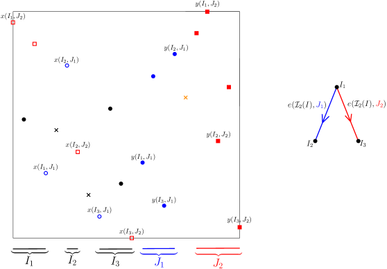
Figure 6.2: In the figure we give an example of a permutation $\pi$ and intervals $I$ and $J$ such that $H({\mathcal{I}}_{2}(I);{\mathcal{I}}_{2}(J))$ is a directed cherry. Take $n=22$, $I=\{1,\ldots,12\}$, $J=\{13,\ldots,22\}$ and permutation $\pi=21,12,19,7,11,17,9,5,3,13,6,1,8,16,4,18,14,20,22,10,15,2$. One may check that ${\mathcal{I}}_{2}(I)=\{I_{1},I_{2},I_{3}\}$ and that ${\mathcal{I}}_{2}(J)=\{J_{1},J_{2}\}$ as shown. For each $i$ the point $(i,\pi(i))$ is plotted with a blue dot if $i\in J_{1}$, a blue circle if $i\in I$ and $\pi(i)+1\in\pi(J_{1})$, a filled red square if $i\in J_{2}$, an empty red square if $i\in I$ and $\pi(i)+1\in\pi(J_{2})$, a black cross if $i\in W_{2}(I)$ and an orange cross if $i\in W_{2}(J)$.

As noted, the vertices of these graphs are elements of ${\mathcal{I}}_{k}(I)$ and $({\mathcal{I}}_{k}(I_{1}),{\mathcal{I}}_{k}(I_{2}))$, respectively. Now, these intervals are of the form $\{i_{k}+1,\ldots,i_{k+1}-1\}$ where $i_{k}$ and $i_{k+1}$ are both elements of $W_{k}(I^{\prime})$ for $I^{\prime}$ equal to one of $I,I_{1}$ or $I_{2}$. Membership in $W_{k}(I^{\prime})$ can be determined via (116). So an interval $\{a,\ldots,b\}$ is an element of for instance ${\mathcal{I}}_{k}(I)$ if and only if $a-1$ and $b+1$ are two consecutive elements of $W_{k}(I)$. Then if we want to check whether $I^{\prime}\in{\mathcal{I}}_{k}(I)$ and $I^{\prime\prime}\in{\mathcal{I}}_{k}(I)$ are connected by an arc, we simply need to check whether there is an interval $J^{\prime}\in{\mathcal{I}}_{k}(J)$ for which $y(I^{\prime},J^{\prime})=\min_{\ell=1,\ldots,|{\mathcal{I}}_{K}(I)|}y(I_{\ell},J^{\prime})$ and $y(I^{\prime\prime},J^{\prime})=\max_{\ell=1,\ldots,|{\mathcal{I}}_{K}(I)|}y(I_{\ell},J^{\prime})$. The elements $y(I_{\ell},J^{\prime})$ can be determined in $\operatorname{\mathsf{TOTO}}$ as we have already seen, and we can compare $y(I_{\ell},J^{\prime})$ and $y(I_{\ell^{\prime}},J^{\prime})$ by the total ordering $<_{1}$.

We need one more ingredient in order to describe the final non–convergent sentence $\varphi$ in Proposition 6.1. Given two disjoint sets $A,B$ we say that a directed graph $G$ with vertex set $A\uplus B$ is a directed matching from $A$ to $B$ if every arc of $G$ connects a vertex in $A$ to a vertex in $B$. Given disjoint intervals $I,I^{\prime}$ we associate to them the intervals ${\mathcal{I}}_{k}(I)=(I_{1},\ldots,I_{N})$, respectively ${\mathcal{I}}_{k}(I^{\prime})=I^{\prime}_{1},\ldots,I^{\prime}_{N^{\prime}}$. We will need to determine if $N>N^{\prime}$. We construct a formula $\mathsf{Bigger}(I,I^{\prime})$ satisfied with high probability by two intervals $I,I^{\prime}$ whenever $N^{\prime}<\log\log n<N<2\log\log n$. This formula may be written in $\operatorname{\mathsf{TOTO}}$ as $\exists a,b$ such that, writing $J\coloneqq(a,b)$, the following holds in $H(({\mathcal{I}}_{k}(I),{\mathcal{I}}_{k}(I^{\prime}));{\mathcal{I}}_{k}(J))$:

• All vertices in ${\mathcal{I}}_{k}(I^{\prime})$ have outdegree $1$;

• All vertices in ${\mathcal{I}}_{k}(I)$ have indegree at most $1$;

• There is a vertex in ${\mathcal{I}}_{k}(I)$ with indegree $0$;

• All arcs start at a vertex in ${\mathcal{I}}_{k}(I)$ and end at a vertex in ${\mathcal{I}}_{k}(I^{\prime})$.

This directed graph is then necessarily a directed matching from ${\mathcal{I}}_{k}(I^{\prime})$ to ${\mathcal{I}}_{k}(I)$ that saturates the vertices in ${\mathcal{I}}_{k}(I^{\prime})$ but not those in ${\mathcal{I}}_{k}(I)$. Such a matching exists if and only if $|{\mathcal{I}}_{k}(I)|>|{\mathcal{I}}_{k}(I^{\prime})|$.

The following two lemmas will be proved in Section 6.4.

Lemma 6.2.

For every fixed $k\geq 3$, with probability $1-e^{-n^{\Omega(1)}}$ there is an interval $I$ with $N\coloneqq|{\mathcal{I}}_{k}(I)|$ satisfying $\log\log n<N<2\log\log n$ such that for every directed graph $G$ with vertex set ${\mathcal{I}}_{k}(I)$ there exists an interval $J\subseteq[n]$ such that

$$H({\mathcal{I}}_{k}(I),{\mathcal{I}}_{k}(J))=G,$$

and moreover $w_{k+1}(I)=0$ and $w_{k-1}(I^{\prime})>0$ for all $I^{\prime}\in{\mathcal{I}}_{k}$.

Lemma 6.3.

For $k$ sufficiently large but not depending on $n$, with probability $1-O(n^{-998})$, for every two disjoint intervals $I_{1},I_{2}\subseteq[n]$ satisfying

• $0<|{\mathcal{I}}_{k}(I_{1})|<\log\log n<|{\mathcal{I}}_{k}(I_{2})|<2\log\log n$;

• $w_{k+1}(I_{1})=w_{k+1}(I_{2})=0$;

• $w_{k-1}(I^{\prime})>0$ for all $I\in{\mathcal{I}}_{k}(I_{1})\cup{\mathcal{I}}_{k}(I_{2})$,

there exists an interval $J$ such that $H(({\mathcal{I}}_{k}(I_{1}),{\mathcal{I}}_{k}(I_{2})),{\mathcal{I}}_{2}(J))$ is a directed matching between ${\mathcal{I}}_{k}(I_{1})$ and ${\mathcal{I}}_{k}(I_{2})$ that saturates ${\mathcal{I}}_{k}(I_{1})$.

6.3 Proof of Proposition 6.1

Given intervals $I$ and $J$ we have seen in the previous section how to define a directed graph on ${\mathcal{I}}_{k}(I)=(I_{1},\ldots,I_{N})$ by selecting an interval $J$. Note that the $I_{i}$ are disjoint intervals, so we inherit a total ordering on them from the $<_{1}$ relation on the domain of $\Pi_{n}$. This allows us in $\operatorname{\mathsf{TOTO}}$ to distinguish for instance $I_{1},I_{2}$ and $I_{N}$.

We will apply the ideas developed in Section 6.1 to sets of the form ${\mathcal{I}}_{k}(I)$. Such sets are subsets of the collection of all intervals in $[n]$, and (given $I$) we can determine membership of an interval $\{a,\ldots,b\}$ in ${\mathcal{I}}_{k}(I)$ by a $\operatorname{\mathsf{TOTO}}$ formula as described in the previous section. This formula will serve as the formula $\eta$ in Section 6.1. Any four intervals $J_{D},J_{E},J_{T},J_{W}$ induce four directed graph structures on ${\mathcal{I}}_{k}(I)$, and we may check whether these graphs satisfy $\mathsf{Arith}$ as given in Section 6.1. If so, then $\mathsf{EvenSize}(J_{D},J_{E},J_{T},J_{W})$ holds if and only if $\log^{**}\log^{**}|{\mathcal{I}}_{k}(I)|$ is even. Lemma 6.2 will allow us to deduce that with high probability there are $J_{D},J_{E},J_{T},J_{W}$ satisfying $\mathsf{Arith}$ so that we can then check the parity of $\log^{**}\log^{**}|{\mathcal{I}}_{k}(I)|$.

We now describe the sentence $\varphi$ appearing in Proposition 6.1. It will be of the form

$$\varphi=\exists x_{1},y_{1},\ldots,x_{5},y_{5}\left(\varphi_{0}\wedge\forall x_{6},y_{6},\ldots,x_{10},y_{10}(\varphi_{1}\to\varphi_{2})\right).$$ (118)

We use the ten pairs of elements to define intervals $I,J_{D},J_{E},J_{T},J_{W},I^{\prime},J_{D}^{\prime},J_{E}^{\prime},J_{T}^{\prime},J_{W}^{\prime}$ by $I=(x_{1},y_{1}),\ldots,J_{W}^{\prime}=(x_{10},y_{10})$. We define $\varphi_{0}(x_{1},y_{1},\ldots,x_{5},y_{5})$ as the $\operatorname{\mathsf{TOTO}}$ formula such that $(\Pi_{n},i_{1},j_{1},\ldots,i_{5},j_{5})\models\varphi_{0}$ if and only if

• $w_{k+1}(I)=0$ and $w_{k-1}(\tilde{I})>0$ for all $\tilde{I}\in{\mathcal{I}}_{k}(I)$;

• $\mathsf{Arith}(I,J_{D},J_{E},J_{T},J_{W})$ is satisfied;

• $\mathsf{EvenSize}(I,J_{D},J_{E},J_{T},J_{W})$ is satisfied.

We define the formula $\varphi_{1}(x_{6},y_{6},\ldots,x_{10},y_{10})$ that holds if and only if the first two conditions above are satisfied but $\mathsf{EvenSize}$ is not satisfied in the induced structure. Finally, we let $\varphi_{2}(x_{1},y_{1},x_{6},y_{6})\coloneqq\mathsf{Bigger}(I,I^{\prime})$.

Proof of Proposition 6.1.

We show that with $\varphi$ as defined in (118), $\Pi_{n}\sim\operatorname{Mallows}(n,1)$ and $n$ satisfying $W^{(2)}(\log^{**}\log^{**}n-1)<{\log\log n}$ we have

$${\mathbb{P}}(\Pi_{n}\models\varphi)=\begin{cases}1-O(n^{-100})&\text{if }\log^{**}\log^{**}n\text{ is even},\\ O(n^{-100})&\text{if }\log^{**}\log^{**}n\text{ is odd}.\end{cases}$$ (119)

In both cases we have by $W^{(2)}(\log^{**}\log^{**}n-1)<{\log\log n}$ and Lemma 3.28 that

$$\log^{**}\log^{**}n-1<\log^{**}\log^{**}\left\lceil\log\log n\right\rceil\leq\log^{**}\log^{**}n.$$ (120)

As the three quantities above are all integers, the second inequality is in fact an equality. Thus, for any integer $m$ satisfying $\log\log n\leq m\leq n$ we have $\log^{**}\log^{**}m=\log^{**}\log^{**}n$.

We let $k$ be such that the conclusion of Lemma 6.3 holds.

Consider first the case $\log^{**}\log^{**}n$ even. By Lemma 6.2 and $\log^{**}\log^{**}m$ being even for all $\log\log n\leq m\leq n$, with probability $1-e^{-n^{\Omega(1)}}$ there exist intervals $I,J_{D},J_{E},J_{T}$ and $J_{W}$ such that $\varphi_{0}(I,J_{D},J_{E},J_{T},J_{W})$ holds and such that $\log\log n<|{\mathcal{I}}_{k}(I)|<2\log\log n$. Now let $I^{\prime},J^{\prime}_{D},J^{\prime}_{E},J^{\prime}_{T}$ and $J^{\prime}_{W}$ be five intervals such that $\varphi_{1}(I^{\prime},J^{\prime}_{D},J^{\prime}_{E},J^{\prime}_{T},J^{\prime}_{W})$ holds (if such intervals do not exist then $\Pi_{n}\models\varphi$ and we are done). Then $N^{\prime}\coloneqq|{\mathcal{I}}_{k}(I^{\prime})|$ must be smaller than ${\log\log n}$, as otherwise $\log^{**}\log^{**}N^{\prime}$ would be even. Thus indeed $N^{\prime}<\log\log n<N<2\log\log n$. By Lemma 6.3, with probability $1-O(n^{-998})$ there exists an interval $J$ such that $H(({\mathcal{I}}_{k}(I),{\mathcal{I}}_{k}(I^{\prime})),J)$ is a directed matching between ${\mathcal{I}}_{k}(I)$ and ${\mathcal{I}}_{k}(I^{\prime})$ that saturates the vertices of ${\mathcal{I}}_{k}(I^{\prime})$ but not the vertices of ${\mathcal{I}}_{k}(I)$. That is, $\mathsf{Bigger}(I,I^{\prime})$ holds with at least this probability. So if $n$ is even ${\mathbb{P}}\left(\Pi_{n}\models\varphi\right)=1-O(n^{-998})$.

We now consider the case $\log^{**}\log^{**}n$ odd. Assume that there are intervals $I,J_{D},J_{E},J_{T},J_{W}$ such that $\varphi_{0}(I,J_{D},J_{E},J_{T},J_{W})$ holds, otherwise we immediately have $\Pi_{n}\not\models\varphi$. We must then have $|{\mathcal{I}}_{k}(I)|<{\log\log n}$. As before, with probability $1-e^{-n^{\Omega(1)}}$ there are $I^{\prime}$, $J^{\prime}_{D}$, $J^{\prime}_{E}$, $J^{\prime}_{T}$ and $J^{\prime}_{W}$ such that $\varphi_{1}(I^{\prime},J^{\prime}_{D},J^{\prime}_{E},J^{\prime}_{T},J^{\prime}_{W})$ holds and $\log\log n<|{\mathcal{I}}_{k}(I^{\prime})|<2\log\log n$. But then $|{\mathcal{I}}_{k}(I^{\prime})|>|{\mathcal{I}}_{k}(I)|$, so $\mathsf{Bigger}(I,I^{\prime})$ cannot be satisfied. ∎

6.4 The probabilistic component

For $B\subseteq[n]$ and $\tau:B\to[n]$ an injection, we will write

$${\mathbb{P}}_{\tau}(.) \coloneqq{\mathbb{P}}(.\,|\,\Pi_{n}(i)=\tau(i)\text{ for all $i\in B$}),$$ (121)

$${\mathbb{E}}_{\tau}(.) \coloneqq{\mathbb{E}}(.\,|\,\Pi_{n}(i)=\tau(i)\text{ for all $i\in B$}).$$ (122)

Recall that we defined

$$w_{k}(A) :=|\{i:\{\Pi_{n}(i),\Pi_{n}(i)+1,\dots,\Pi_{n}(i)+k-1\}\subseteq\Pi_{n}(A)\}|.$$ (123)

We define for the remainder of this section

$$Y_{i}(A)\coloneqq\mathbf{1}_{\{\{i,\ldots,i+k-1\}\,\subseteq\,\Pi_{n}(A)\}}.$$ (124)

We note that $w_{k}(A)=Y_{1}(A)+\ldots+Y_{n-k+1}(A)$.

Lemma 6.4.

If $k$ is fixed, and $A,B\subseteq[n]$ are disjoint sets of cardinality $1\ll|A|\ll n$ and $|B|\,\leq\,n/\log n$, and $\tau:B\to[n]$ is an arbitrary injection, then

$$\begin{array}[]{l}{\mathbb{E}}_{\tau}w_{k}(A)=(1+o(1))n^{1-k}|A|^{k},\\ \\ {\mathbb{E}}_{\tau}w_{k}(A)^{2}\leq\left({\mathbb{E}}_{\tau}w_{k}(A)\right)^{2}+(2k-1)\cdot{\mathbb{E}}_{\tau}w_{k}(A).\end{array}$$

(where the $o(.)$ is uniform over all such $B$ and $\tau$.)

Proof.

Let us denote by $J$ the set of all $1\leq j\leq n-k+1$ for which $\{j,\dots,j+k-1\}\cap\text{Im}(\tau)=\varnothing$. We note that

$${\mathbb{E}}_{\tau}Y_{j}=\left\{\begin{array}[]{cl}\frac{|A|(|A|-1)\dots(|A|-k+1)}{(n-|B|)\dots(n-|B|-k+1)}&\text{ if $j\in J$, }\\ 0&\text{ otherwise.}\end{array}\right..$$

Hence

$${\mathbb{E}}_{\tau}w_{k}(A)=|J|\cdot\frac{|A|(|A|-1)\dots(|A|-k+1)}{(n-|B|)\dots(n-|B|-k+1)}=(1+o(1))\cdot n^{1-k}|A|^{k},$$

using that $|B|\,\leq\,n/\log n$ and $(n-k(|B|+1))\leq|J|\leq n$. The $o(1)$ term above is uniform for all $B$ by the uniform bound $B\,\leq\,n/\log n$.

For the second moment, we remark that

$${\mathbb{E}}_{\tau}Y_{i}Y_{j}=\left\{\begin{array}[]{cl}\frac{|A|(|A|-1)\dots(|A|-2k+1)}{(n-|B|)\dots(n-|B|-2k+1)}&\text{ if $i,j\in J$ and $|i-j|>k$, }\\ 0&\text{ if }i\not\in J\text{ or }j\not\in J,\\ \leq{\mathbb{E}}_{\tau}Y_{i}&\text{ if }|i-j|\leq k.\end{array}\right.$$ (125)

and we also remark that

$$\frac{|A|(|A|-1)\dots(|A|-2k+1)}{(n-|B|)\dots(n-|B|-2k+1)}\leq\left(\frac{|A|(|A|-1)\dots(|A|-k+1)}{(n-|B|)\dots(n-|B|-k+1)}\right)^{2},$$

since $1\ll|A|,|B|\ll n$ so that $(|A|-x)/(n-|B|-x)\leq(|A|-x-1)/(n-|B|-x-1)$ for all $x=1,\dots,2k-1$.

We see that

$$\begin{array}[]{rcl}{\mathbb{E}}_{\tau}w_{k}(A)^{2}&=&\sum_{i}\sum_{j}{\mathbb{E}}_{\tau}Y_{i}Y_{j}\\[4.0pt] &\leq&|J|^{2}\frac{|A|(|A|-1)\dots(|A|-2k+1)}{(n-|B|)\dots(n-|B|-2k+1)}+(2k-1)\sum_{i}{\mathbb{E}}_{\tau}Y_{i}\\[4.0pt] &\leq&\left({\mathbb{E}}_{\tau}w_{k}(A)\right)^{2}+(2k-1)\cdot{\mathbb{E}}_{\tau}w_{k}(A).\end{array}$$

∎

The following lemmas establish that if $w_{k}(I)>0$ then $I$ is large in some suitable sense and if $w_{k}(I)=0$ then $I$ is small.

Lemma 6.5.

For each fixed $k\geq 2$, with probability $1-O(n^{-998})$, for every interval $I\subseteq[n]$ of length at most $n^{1-1000/k}$ we have $w_{k}(I)=0$.

Proof.

It suffices to show the result for all intervals $I$ of length $\left\lfloor n^{1-1000/k}\right\rfloor$ as $w_{k}(I)=0$ implies $w_{k}(I^{\prime})=0$ for all $I^{\prime}\subseteq I$. By Markov’s inequality and Lemma 6.4 with $B=\varnothing$ we have for any given interval $I\subseteq[n]$ with $|I|=\left\lfloor n^{1-1000/k}\right\rfloor$ that

$${\mathbb{P}}\left(w_{k}(I)>0\right)\leq{\mathbb{E}}w_{k}(I)=(1+o(1))n^{1-k}|I|^{k}\leq(1+o(1))n^{1-k}n^{k-1000}=O\left(n^{-999}\right).$$ (126)

There are $O(n)$ intervals in $[n]$ of length $\left\lfloor n^{1-1000/k}\right\rfloor$, so the union bound gives the desired result. ∎

Lemma 6.6.

For each fixed $k$ and $0<\varepsilon<1/k$, with probability at least $1-e^{-\Omega(n^{1-k\varepsilon})}$, every interval $I\subseteq[n]$ of length at least $\left\lceil n^{1-\varepsilon}\right\rceil$ satisfies $w_{k}(I)>0$.

Proof.

Since there are $O(n^{2})$ possible intervals, it is enough to show that for any fixed interval $I$ of length $\left\lceil n^{1-\varepsilon}\right\rceil$ we have ${\mathbb{P}}(w_{k}(I)=0)\leq e^{-\Omega(n^{1-k\varepsilon})}$.

So let $I\subseteq[n]$ be an interval of length $|I|=\left\lceil n^{1-\varepsilon}\right\rceil$. Let $J\subseteq[n]$ be a random subset where we independently include $i$ in $J$ with probability

$${\mathbb{P}}\left(i\in J\right)=\frac{|I|}{n},\quad\text{for all }i\in[n].$$ (127)

Denote by $E$ the event $\{|J|=|I|\}$. By Lemma 3.3 we have ${\mathbb{P}}\left(E\right)\geq 1/(n+1)$. Recall the definition of $Y_{j}(I)$ in (124), define for $1\leq j\leq n-k+1$ also the random variable

$$X_{j} \coloneqq\mathbf{1}_{\{\{j,\ldots,j+k-1\}\,\subseteq\,J\}}.$$ (128)

If $E$ holds then $J\hskip 0.86108pt\raisebox{-0.43057pt}{$=$}\raisebox{4.30554pt}{{$\scriptstyle d$}}\hskip 3.44444pt\Pi_{n}(I)$, namely, both are uniformly selected random subsets of $[n]$ of size $|I|$ if $E$ occurs. Thus

$${\mathbb{P}}\left(w_{k}(I)=0\right)={\mathbb{P}}\left(\bigcap_{j}\,\overline{Y_{j}}\right)={\mathbb{P}}\left(\bigcap_{j}\,\overline{X_{j}}\,\Bigg{|}\,E\right)=\frac{{\mathbb{P}}\left(\bigcap_{j}\,\overline{X_{j}}\cap E\right)}{{\mathbb{P}}\left(E\right)}\leq(n+1)\,{\mathbb{P}}\left(\bigcap_{j}\,\overline{X_{j}}\right).$$ (129)

Let $S=\{ki:i\in{\mathbb{N}}\}\cap[n-k+1]$. The $X_{j}$ are independent for $j\in S$, and if $X_{j}$ is to occur for no $j\in[n-k+1]$ then certainly $X_{j}$ should not occur for any $j\in S$. Therefore

$${\mathbb{P}}\left(w_{k}(I)=0\right) \leq(n+1)\left(1-\frac{|I|^{k}}{n^{k}}\right)^{|S|}\leq(n+1)\exp\left\{-|S|\frac{|I|^{k}}{n^{k}}\right\}.$$ (130)

By $|S|=(1+o(1))n/k$ and $|I|/n\geq n^{-\varepsilon}$ we conclude that

$${\mathbb{P}}\left(w_{k}(I)=0\right) \leq\exp\left\{-(1+o(1))\frac{n^{1-k\varepsilon}}{k}\right\}.$$ (131)

∎

Lemma 6.7.

For $k\geq 3$ and $\varepsilon>0$, let $I\subseteq[n]$ be an interval of length $\lfloor n^{1-1/k}\cdot\left(\log\log n\right)^{3/k}\rfloor$, and let $B\subseteq[n]$ be disjoint from $I$ with $|B|\ll n/\log n$ and let $\tau:B\to[n]$ be an arbitrary injection. Let $E$ denote the event that

1. $(1-\varepsilon)\left(\log\log n\right)^{3}<w_{k}(I)<(1+\varepsilon)\left(\log\log n\right)^{3}$, and;

2. $w_{k+1}(I)=0$, and;

3. $w_{k-1}(I^{\prime})>0$ for each $I^{\prime}\in{\mathcal{I}}_{k}(I)$, and;

4. $|I^{\prime}|>n^{4/7}$ for all $I^{\prime}\in{\mathcal{I}}_{k}(I)$.

Then ${\mathbb{P}}_{\tau}(E)=1-o(1)$, where the $o(1)$ term is uniform over the choice of $B$ and $\tau$.

Proof.

By Chebyshev’s inequality and Lemma 6.4 we have

$${\mathbb{P}}_{\tau}\left(\left|w_{k}(I)-{\mathbb{E}}_{\tau}w_{k}(I)\right|>\frac{\varepsilon}{2}(\log\log n)^{3}\right) \leq\frac{(2k-1){\mathbb{E}}_{\tau}w_{k}(I)}{\left(\frac{\varepsilon}{2}(\log\log n)^{3}\right)^{2}},$$ (132)

where

$${\mathbb{E}}_{\tau}w_{k}(I)=(1+o(1))n^{1-k}|I|^{k}=(1+o(1))(\log\log n)^{3}.$$ (133)

Thus

$${\mathbb{P}}_{\tau}\left(\left|w_{k}(I)-(1+o(1))(\log\log n)^{3}\right|>\frac{\varepsilon}{2}(\log\log n)^{3}\right)<\frac{8k}{\varepsilon^{2}(\log\log n)^{3}}=o(1),$$ (134)

showing Part (i).

A simple application of Markov’s inequality together with Lemma 6.4 gives

$${\mathbb{P}}_{\tau}\left(w_{k+1}(I)>0\right)\leq{\mathbb{E}}_{\tau}w_{k+1}(I)=(1+o(1))n^{-k}\left(n^{1-\frac{1}{k}}(\log\log n)^{\frac{3}{k}}\right)^{k+1}=o(1),$$ (135)

giving Part (ii).

We now look at Parts (iii) and (iv). We first show the stronger claim that for any fixed $\delta>1/k$ we have

$${\mathbb{P}}\left(|I^{\prime}|\geq n^{1-\delta}\text{ for all }I^{\prime}\in{\mathcal{I}}_{k}(I)\right)=1-o(1).$$ (136)

Then Part (iii) will follow from Lemma 6.6 with e.g. $\delta=\frac{1}{2}(\frac{1}{k}+\frac{1}{k-1})$ satisfying $\frac{1}{k}<\delta<\frac{1}{k-1}$, and Part (iv) will follow by setting $\delta=\frac{3}{7}$. Note that $w_{k}(I)$ depends only on the image $\Pi_{n}[I]$. Conditioning on $\Pi_{n}[I]=I^{\prime}$ for some $I^{\prime}\subseteq[n]$, $\Pi_{n}\upharpoonright I$ is distributed uniformly over all bijections $I\to I^{\prime}$. So conditional on the value of $w_{k}(I)$, $W_{k}(I)$ is a subset of $I$ of size $w_{k}(I)$ selected uniformly at random. Let $F$ be the event $\{w_{k}(I)<2(\log\log n)^{3}\}$. Conditional on $F$, the probability that $|I^{\prime}|<n^{1-\delta}$ for some $I^{\prime}\in{\mathcal{I}}_{k}(I)$ is at most the probability that out of $2(\log\log n)^{3}$ points selected uniformly at random from $I$, there is a pair $i,j$ with $|i-j|\leq n^{1-\delta}$. There are at most $|I|\,n^{1-\delta}$ candidates for such $i,j$. Thus

$${\mathbb{P}}\left(\left.\exists i,j\in W_{k}(I)\text{ s.t. }|i-j|\leq n^{1-\delta}\,\right|\,F\right) \leq|I|\,n^{1-\delta}\,O\left(\frac{4(\log\log n)^{6}}{|I|^{2}}\right)$$ (137)

$$=\frac{n^{1-\delta+o(1)}}{|I|}$$ (138)

$$=n^{-\delta+\frac{1}{k}+o(1)}.$$ (139)

For $\delta>\frac{1}{k}$ this is indeed $o(1)$. We finish the proof by noting that by Part (i), ${\mathbb{P}}\left(F\right)=1-o(1)$. ∎

Corollary 6.8.

Let $k\geq 3$ be arbitrary, $0<\varepsilon<1/k$ and let $I_{1},\dots,I_{N}$ be disjoint intervals of length $\lfloor n^{1-1/k}\cdot\left(\log\log n\right)^{3/k}\rfloor$ where $N=\left\lceil n^{\varepsilon}\right\rceil$. With probability $1-e^{-\Omega(n^{\varepsilon})}$, at least half of the $I_{i}$ satisfy properties (i)-(iv) of Lemma 6.7.

Proof.

Let $E_{i}$ denote the event that $I_{i}$ satisfies properties (i)-(iv) of Lemma 6.7. Let $S\subseteq[N]$, we will look at the probability that $E_{i}$ does not hold for some $i\in S$. Let $g(n)$ be a function going to zero such that ${\mathbb{P}}_{\tau}\left(E_{i}\right)\geq 1-g(n)$ for any $i\in S$, $B\subseteq\bigcup_{j\in S}I_{j}\setminus\{I_{i}\}$ and any injection $\tau:B\to[n]$. Such a $g$ exists by Lemma 6.7 and $\sum|I_{j}|\ll n/\log n$. Then

$${\mathbb{P}}\left(\bigcap_{i\in S}\,\overline{E_{i}}\right)=\prod_{i\in S}{\mathbb{P}}\left(\overline{E_{i}}\,\left|\,\bigcap_{j\in S,j<i}\overline{E_{j}}\right.\right).$$ (140)

The event $\bigcap_{j\in S,j<i}\overline{E_{j}}$ depends only on the restriction of $\Pi_{n}$ to $\bigcup_{j\in S,j<i}I_{j}$. But for any such $\tau:\bigcup_{j\in S,j<i}I_{j}\to[n]$ we have ${\mathbb{P}}_{\tau}\left(\overline{E_{i}}\right)\leq g(n)$. Thus ${\mathbb{P}}\left(\bigcap_{i\in S}\,\overline{E_{i}}\right)\leq g(n)^{|S|}.$ By Theorem 3.2 with $\gamma=\frac{1}{2}>g(n)$ we have

$${\mathbb{P}}\left(\sum_{i=1}^{N}\overline{E_{i}}\geq\frac{N}{2}\right)\leq\exp\left\{-2N\left(\frac{1}{2}-g(n)\right)^{2}\right\}=\exp\left\{-\frac{(1-o(1))n^{\varepsilon}}{2}\right\}.$$ (141)

∎

Lemma 6.9.

Let $I$ be an interval satisfying Conditions (ii)-(iv) of Lemma 6.7. Let $J$ be obtained from $I$ by deleting its largest element. Then $J$ satisfies Conditions (ii)-(iv) of Lemma 6.7 and

$$|{\mathcal{I}}_{k}(I)|-k\leq|{\mathcal{I}}_{k}(J)|\leq|{\mathcal{I}}_{k}(I)|.$$ (142)

Proof.

Note that $W_{t}(J)\subseteq W_{t}(I)$ for all $t\geq 1$, so that $w_{k+1}(I)=0$ implies $w_{k+1}(J)=0$. Now let $J^{\prime}\in{\mathcal{I}}_{k}(J)$, then $J^{\prime}=\{a+1,\ldots,b-1\}$ with $a,b\in W_{k-1}(J)\subseteq W_{k-1}(I)$. Then either $J^{\prime}\in{\mathcal{I}}_{k}(I)$ or $J^{\prime}\supsetneq I^{\prime}$ for some $I^{\prime}\in{\mathcal{I}}_{k}(I)$. In the latter case, such $I^{\prime}$ satisfies Conditions (iii) and (iv) of Lemma 6.7 so $J^{\prime}$ does as well.

We now show (142). Define $j$ to be the largest element in $I$. Then there are at most $k$ elements $i\in I$ such that $\Pi_{n}(j)\in\{\Pi_{n}(i),\ldots,\Pi_{n}(i)+k-1\}$. Thus $|W_{k}(I)\setminus W_{k}(J)|\leq k$. ∎

Recall that we defined

$$S(I,J)=\{i:i\in\Pi_{n}(I),i+1\in\Pi_{n}(J)\}.$$ (143)

Lemma 6.10.

Let $\varepsilon,\delta>0$ be arbitrary (but fixed). With probability at least $1-e^{-n^{\Omega(1)}}$, for every two disjoint intervals $I_{1},I_{2}\subseteq[n]$ of length at least $n^{\frac{1}{2}+\varepsilon}$, we have

$$(1-\delta)\cdot\frac{|I_{1}|\cdot|I_{2}|}{n}\leq|S(I_{1},I_{2})|\leq(1+\delta)\cdot\frac{|I_{1}|\cdot|I_{2}|}{n}.$$

Proof.

Fix disjoint intervals $I_{1},I_{2}$ of the stated sizes. Note $J_{1}:=\Pi_{n}(I_{1}),J_{2}:=\Pi_{n}(I_{2})$ are disjoint, random sets of cardinalities exactly $|I_{1}|$, resp. $|I_{2}|$, every pair of disjoint sets of the correct cardinalities being equally likely.

We approximate these by sets with a random number of elements, generated as follows. Write $p_{i}:=|I_{i}|/n$ for $i=1,2$. Let $Z_{1},\dots,Z_{n}$ be i.i.d. with common distribution given by

$${\mathbb{P}}(Z_{j}=x)=\left\{\begin{array}[]{cl}1-(p_{1}+p_{2})&\text{ if $x=0$, }\\ p_{1}&\text{ if $x=1$, }\\ p_{2}&\text{ if $x=2$. }\\ \end{array}\right.$$

We now set $J_{1}^{\prime}:=\{j:Z_{j}=1\},J_{2}^{\prime}:=\{j:Z_{j}=2\}$. Conditional on the event

$$E:=\{|J_{1}^{\prime}|=|I_{1}|,|J_{2}^{\prime}|=|I_{2}|\},$$

the pair $(J_{1}^{\prime},J_{2}^{\prime})$ has the same distribution as $(J_{1},J_{2})$, namely uniform over all pairs of disjoint sets of the correct cardinalities $|I_{1}|$ and $|I_{2}|$. Lemma 3.3 gives the crude bound

$${\mathbb{P}}(E)={\mathbb{P}}\left(|J^{\prime}_{1}|=|I_{1}|\right){\mathbb{P}}\left(|J_{2}^{\prime}|=|I_{2}|\,|\,|J^{\prime}_{1}|=|I_{1}|\right)\geq\frac{1}{(n+1)^{2}}.$$ (144)

Next, we consider the size of

$$S^{\prime}\coloneqq\{j:j\in J_{1}^{\prime},j+1\in J_{2}^{\prime}\}.$$

Write $X_{j}:=\mathbf{1}_{\{j\in S^{\prime}\}}$, so that $|S^{\prime}|=X_{1}+\dots+X_{n-1}$. We have ${\mathbb{E}}X_{j}=p_{1}p_{2}=:p$ and

$${\mathbb{E}}|S^{\prime}|=(n-1)p=\frac{|I_{1}|\cdot|I_{2}|}{n}-p.$$ (145)

In particular ${\mathbb{E}}|S^{\prime}|=(1+o(1))n^{2\varepsilon}$ by our assumption on the sizes $|I_{1}|,|I_{2}|\geq n^{1/2+\varepsilon}$. Now $|S^{\prime}|$ is not a binomial random variable as the $X_{j}$ are (mildly) dependent – it is for instance not possible to have two consecutive integers in $S^{\prime}$. Note that $X_{j}$ is however (mutually) independent from the collection of all $X_{i}$ with $|i-j|\geq 2$. So, writing

$$X_{\text{even}}:=\sum_{j\text{ even}}X_{j},\quad X_{\text{odd}}:=\sum_{j\text{ odd}}X_{j},$$

we see that $|S^{\prime}|=X_{\text{even}}+X_{\text{odd}}$ and $X_{\text{even}}\hskip 0.86108pt\raisebox{-0.43057pt}{$=$}\raisebox{4.30554pt}{{$\scriptstyle d$}}\hskip 3.44444pt\operatorname{Bi}(\lfloor(n-1)/2\rfloor,p),X_{\text{odd}}\hskip 0.86108pt\raisebox{-0.43057pt}{$=$}\raisebox{4.30554pt}{{$\scriptstyle d$}}\hskip 3.44444pt\operatorname{Bi}(\lceil(n-1)/2\rceil,p)$. By the Chernoff bound we have

$${\mathbb{P}}\left(|X_{\text{even}}-{\mathbb{E}}X_{\text{even}}|\geq\frac{\delta}{100}\cdot{\mathbb{E}}X_{\text{even}}\right)\leq e^{-\Omega({\mathbb{E}}X_{\text{even}})}=e^{-\Omega(np)}=e^{-n^{\Omega(1)}},$$

and analogously ${\mathbb{P}}(|X_{\text{odd}}-{\mathbb{E}}X_{\text{odd}}|\geq\frac{\delta}{100}\cdot{\mathbb{E}}X_{\text{odd}})=e^{-n^{\Omega(1)}}$. It follows that

$${\mathbb{P}}\left(\left||S^{\prime}|-{\mathbb{E}}|S^{\prime}|\right|\geq\frac{\delta}{100}{\mathbb{E}}|S^{\prime}|\right)\leq e^{-n^{\Omega(1)}}.$$ (146)

We see that

$$\begin{array}[]{rcl}{\mathbb{P}}\left(\left|S-\frac{|I_{1}|\cdot|I_{2}|}{n}\right|>\delta\frac{|I_{1}|\cdot|I_{2}|}{n}\right)&\leq&{\mathbb{P}}\left(|S-{\mathbb{E}}S^{\prime}|>\frac{\delta}{100}{\mathbb{E}}|S^{\prime}|\right)\\[2.0pt] &=&{\mathbb{P}}\left(|S^{\prime}-{\mathbb{E}}S^{\prime}|>\frac{\delta}{100}{\mathbb{E}}|S^{\prime}||E\right)\\[2.0pt] &=&{\mathbb{P}}\left(\left\{|S^{\prime}-{\mathbb{E}}S^{\prime}|>\frac{\delta}{100}{\mathbb{E}}|S^{\prime}|\right\}\cap E\right)/{\mathbb{P}}(E)\\[2.0pt] &\leq&{\mathbb{P}}\left(|S^{\prime}-{\mathbb{E}}S^{\prime}|>\frac{\delta}{100}{\mathbb{E}}|S^{\prime}|\right)/{\mathbb{P}}(E)\\[2.0pt] &\leq&(n+1)^{2}\cdot e^{-n^{\Omega(1)}}\\[4.0pt] &=&e^{-n^{\Omega(1)}}.\end{array}$$

(Here the first inequality holds for $n$ sufficiently large and uses (145). In the second line we use the earlier observation that $(S^{\prime}|E)\hskip 0.86108pt\raisebox{-0.43057pt}{$=$}\raisebox{4.30554pt}{{$\scriptstyle d$}}\hskip 3.44444ptS$ and in the fifth line we use (144) and (146).) ∎

Lemma 6.11.

For every fixed $\varepsilon>0$ and $k\geq 3$, with probability $1-e^{-n^{\Omega(1)}}$, for every sequence ${\mathcal{I}}=(I_{1},\dots,I_{N})$ of at most $10\log\log n$-many disjoint intervals satisfying

$$n^{\frac{1}{2}+\varepsilon}\leq|I_{1}|,\dots,|I_{N}|\leq n^{1-\varepsilon},$$

and every directed graph $G$ with $V(G)=\{I_{1},\ldots,I_{N}\}$, there exists an interval $J\subseteq[n]$ such that

$$H({\mathcal{I}};{\mathcal{I}}_{k}(J))=G.$$

Proof.

There are no more than $10\log\log n\cdot n^{20\log\log n}=e^{O\left(\log n\cdot\log\log n\right)}$ many ways to pick $I_{1},\dots,I_{N}$, and at most $2^{O((\log\log n)^{2})}$ corresponding directed graphs $G$ for each such a sequence. We will show that for each particular choice of $I_{1},\dots,I_{N}$ and $G$ with $v(G)=N$, the probability that no $J$ exists as desired is at most $e^{-n^{\Omega(1)}}$. This will prove the lemma.

Let us thus fix $I_{1},\dots,I_{N}$, meeting the conditions of the lemma but otherwise arbitrary, and an arbitrary directed graph $G$ on $N$ vertices. Note that if $G$ is the “empty directed graph” ($e(G)=0$) then we can simply take $J=\{1\}$. Thus, we can and do assume from now on that $G$ has at least one arc.

Inside the set $[n]\setminus(I_{1}\cup\dots\cup I_{N})$ we can find $M=n^{\Omega(1)}$ disjoint intervals $J_{1},\dots,J_{M}$ each of size $s:=\lceil n^{1-1/k}\cdot\left(\log\log n\right)^{3/k}\rceil$.

For $\tau:I_{1}\cup\dots\cup I_{N}\to[n]$ an injection and $L_{1},\dots,L_{M}\geq 0$ and $A_{11},\dots,A_{1L_{1}}\subseteq J_{1}$, $\dots$, $A_{M1},\dots,A_{ML_{M}}\subseteq J_{M}$ disjoint intervals, and $B_{11},\dots,B_{1L_{1}},\dots,B_{ML_{M}}\subseteq[n]\setminus\tau[I_{1}\cup\dots\cup I_{N}]$ disjoint sets with $|A_{ij}|=|B_{ij}|$ for all $i,j$, we define the event

$$F_{\tau,\underline{A},\underline{B}}:=\left\{\begin{array}[]{l}{\mathcal{I}}_{k}(J_{\ell})=(A_{\ell 1},\dots,A_{\ell L_{\ell}})\text{ for all $\ell=1,\dots,M$, }\\ \Pi_{n}[A_{\ell\ell^{\prime}}]=B_{\ell\ell^{\prime}}\text{ for all $\ell=1,\dots,M$ and $\ell^{\prime}=1,\dots,L_{\ell}$, }\\ \Pi_{n}(x)=\tau(x)\text{ for all $x\in I_{1}\cup\dots\cup I_{n}$.}\end{array}\right\}$$

We observe that, conditional on $F_{\tau,\underline{A},\underline{B}}$, every bijection $A_{ij}\to B_{ij}$ is equally likely. That is, for every choice of bijections $\tau_{11}:A_{11}\to B_{11},\dots,\tau_{ML_{M}}:A_{ML_{M}}\to B_{ML_{M}}$ we have

$${\mathbb{P}}\left(\text{$\Pi_{n}\upharpoonright A_{ij}\equiv\tau_{ij}$ for all $i,j$}{\big{|}}F_{\tau,\underline{A},\underline{B}}\right)=\frac{1}{|A_{11}|!\cdot\dots\cdot|A_{ML_{M}}|!}.$$

Let us say an index $1\leq\ell\leq M$ is good if $(1-\varepsilon)(\log\log n)^{3}\leq L_{\ell}\leq(1+\varepsilon)(\log\log n)^{3}$ and $S(I_{i},J^{\prime})>0$ for all $1\leq i\leq N$ and $J^{\prime}\in{\mathcal{I}}_{k}(J_{\ell})$. (So in particular $H({\mathcal{I}},{\mathcal{I}}_{k}(J_{\ell}))$ is defined when $\ell$ is good.) Note also that whether $\ell$ is good or not is determined completely by $F_{\tau,\underline{A},\underline{B}}$, because the sets $S(I_{i},A_{\ell j})$ depend only on $B_{\ell j}$, not on the choice of the specific bijection $A_{\ell j}\to B_{\ell j}$.

Note that if $\ell$ is good and we randomly choose bijections $\tau_{i\ell}:A_{i\ell}\to B_{i\ell}$ then the points $y(I_{1},A_{i\ell}),\dots,y(I_{N},A_{i\ell})$ are chosen uniformly without replacement from $A_{i\ell}$. In particular, defining $P\coloneqq\{(I_{i},I_{j}):i\neq j\}$, for each ordered pair $uv\in P$ the probability that $e({\mathcal{I}},A_{i\ell})=uv$ is $\frac{1}{|P|}=\frac{1}{N(N-1)}$.

We fix a sequence $e_{1},e_{2},\dots,e_{\lceil(1+\varepsilon)(\log\log n)^{3}\rceil}\in P$ with the property that

$$E(G)=\{e_{1},\dots,e_{\lceil(1-\varepsilon)(\log\log n)^{3}\rceil}\}=\{e_{1},\dots,e_{\lceil(1+\varepsilon)(\log\log n)^{3}\rceil}\}.$$

Since $(1-\varepsilon)(\log\log n)^{3}n>N^{2}$, there are necessarily some duplicate arcs, this will not be a problem. Then $H({\mathcal{I}},(A_{\ell 1},\dots,A_{\ell L_{\ell}}))=G$ is implied by the event $\{e({\mathcal{I}},A_{\ell i})=e_{i}\text{ for all $1\leq i\leq L_{i}$}\}$.

For notational convenience, let us write

$$E:=\{H({\mathcal{I}},{\mathcal{I}}_{k}(J_{\ell}))=G\text{ for some $1\leq\ell\leq M$ }\}.$$

It follows from the previous observations that if $Z$ denotes the number of good indices, then the value of $Z$ is completely determined by the event $F_{\tau,\underline{A},\underline{B}}$, and

$$\begin{array}[]{rcl}{\mathbb{P}}\left(E|F_{\tau,\underline{A},\underline{B}}\right)&\geq&\displaystyle 1-\left(1-\left(\frac{1}{N^{2}}\right)^{(1+\varepsilon)(\log\log n)^{3}}\right)^{Z}\\[8.61108pt] &\geq&\displaystyle 1-\exp\left[-Z\cdot\left(\frac{1}{N^{2}}\right)^{(1+\varepsilon)(\log\log n)^{3}}\right]\\[12.91663pt] &=&\displaystyle 1-\exp\left[-Z\cdot n^{o(1)}\right].\end{array}$$

By Corollary 6.8 and Lemma 6.10 we have that

$${\mathbb{P}}(Z<M/2)=e^{-n^{\Omega(1)}}.$$

It follows that

$$\begin{array}[]{rcl}{\mathbb{P}}(E)&\geq&\displaystyle\sum_{\tau,\underline{A},\underline{B}}{\mathbb{P}}\left(E|F_{\tau,\underline{A},\underline{B}}\right)\cdot{\mathbb{P}}(F_{\tau,\underline{A},\underline{B}})\\ &\geq&\displaystyle 1-\exp[-M/2]-{\mathbb{P}}(Z<M/2)\\ &=&1-e^{-n^{\Omega(1)}}.\end{array}$$

This proves the statement of the lemma. ∎

Proof of Lemma 6.2.

Let $I_{1},\ldots,I_{N}$ be $\left\lceil n^{1/2k}\right\rceil$ intervals of length $\lfloor n^{1-1/k}\cdot\left(\log\log n\right)^{3/k}\rfloor$. By Corollary 6.8, with probability $1-e^{-\Omega(n^{1/2k})}$ at least $1$ of them satisfies Conditions (i)-(iv) of Lemma 6.7, by relabeling if necessary, we can assume that $I_{1}$ satisfies these conditions. We have ${\mathcal{I}}_{k}(I_{1})\gg\log\log n$ by Condition (i). By Lemma 6.9 we may shrink $I_{1}$ by iteratively removing the maximum element until $\log\log n<|{\mathcal{I}}_{k}(I_{1})|<2\log\log n$, ensuring that $I_{1}$ still satisfies Conditions (ii)-(iv) of Lemma 6.7. In particular $|I^{\prime}|>n^{4/7}$ for all $I^{\prime}\in{\mathcal{I}}_{k}(I_{1})$, and by $|I_{1}|\leq n^{1-1/2k}$ we also have $I^{\prime}\leq n^{1-1/2k}$ for all $I^{\prime}\in{\mathcal{I}}_{k}(I_{1})$.

By Lemma 6.11, for all directed graphs $G$ with $V(G)={\mathcal{I}}_{k}(I_{1})$ there is an interval $J$ satisfying $H({\mathcal{I}}_{k}(I_{1}),{\mathcal{I}}_{k}(J))=G$, with probability $1-e^{-n^{\Omega(1)}}$. ∎

Proof of Lemma 6.3.

Let $I_{1},I_{2}$ be any two disjoint intervals such that $0<|{\mathcal{I}}_{k}(I_{1})|<\log\log n<|{\mathcal{I}}_{k}(I_{2})|<2\log\log n$, and such that $w_{k+1}(I_{1})=w_{k+1}(I_{2})=0$ and $w_{k-1}(I^{\prime})>0$ for all $I\in{\mathcal{I}}_{k}(I_{1})\cup{\mathcal{I}}_{k}(I_{2})$. Each of these $I^{\prime}\in{\mathcal{I}}_{k}(I_{1})\cup{\mathcal{I}}_{k}(I_{2})$ has length at most $\max\{|I_{1}|,|I_{2}|\}$. By Lemma 6.6 with $\varepsilon=\frac{1}{2(k+1)}$

$${\mathbb{P}}\left(w_{k+1}(I^{\prime})>0\text{ for all intervals }I^{\prime}\text{ s.t. }|I^{\prime}|>n^{1-\frac{1}{2(k+1)}}\right)\geq 1-e^{-\Omega(n^{1/2})}.$$ (147)

So with at least this probability, all $I_{1}$ and $I_{2}$ as described satisfy $|I_{1}|,|I_{2}|\leq n^{1-\frac{1}{2(k+1)}}$. By $w_{k-1}(I^{\prime})>0$ for all $I^{\prime}\in{\mathcal{I}}_{k}(I_{1})\cup{\mathcal{I}}_{k}(I_{2})$ and Lemma 6.5 we have $|I^{\prime}|\geq n^{1-1000/{(k-1)}}$ for all such $I_{1},I_{2}$ and $I^{\prime}\in{\mathcal{I}}_{k}(I_{1})\cup{\mathcal{I}}_{k}(I_{2})$ with probability $1-O(n^{-998})$. So for sufficiently large $k$ we have

$$n^{\frac{1}{2}+\frac{1}{2(k+1)}}<n^{1-1000/(k-1)}\leq|I^{\prime}|<n^{1-\frac{1}{2(k+1)}}.$$ (148)

The result then follows by $|{\mathcal{I}}_{k}(I_{1})\cup{\mathcal{I}}_{k}(I_{2})|\leq 3\log\log n$ and Lemma 6.11. ∎

7 Proof of Theorem 1.2 Part (ii)

Here we extend the case $q=1$ to $|1-q|<1/\log^{*}n$. We will make frequent use of the sampling algorithm for a $\operatorname{Mallows}(n,q)$ distribution detailed in Section 3.2.1. Recall also the definition of $\operatorname{TruncGeo}(n,p)$ random variables whose probability mass function is given in (11) and is valid in the range $p\in(-\infty,0)\cup(0,1)$. In particular, $\operatorname{TruncGeo}(n,1-q)$ random variables are well defined for $q\in{\mathbb{R}}_{>0}\setminus\{1\}$.

7.1 Extending the $q=1$ case to $q=1\pm O(n^{-4})$

We first extend Proposition 6.1 to the following:

Proposition 7.1.

There exists a $\varphi\in{\operatorname{\mathsf{TOTO}}}$ such that for $\Pi_{n}\sim\operatorname{Mallows}(n,q)$, all $n$ satisfying $W^{(2)}(\log^{**}\log^{**}n-1)<\log\log n$ and all $c>0$ we have

$${\mathbb{P}}(\Pi_{n}\models\varphi)=\begin{cases}1-O(cn^{-2})&\text{if }\log^{**}\log^{**}n\text{ is even},\\ O(cn^{-2})&\text{if }\log^{**}\log^{**}n\text{ is odd}.\end{cases}$$ (149)

for all sequences $q=q(n)$ satisfying $0\leq|1-q|\leq cn^{-4}$.

Proposition 6.1 will follow by showing that for $q=1-O(n^{-4})$, a $\operatorname{Mallows}(n,q)$ distribution is in some sense very close to the uniform distribution over $S_{n}$.

Lemma 7.2.

Let $q$ satisfy $0\neq|1-q|\leq cn^{-4}$ for some $c>0$. For $1\leq i\leq n$ let $Z_{i}\sim\operatorname{TruncGeo}(n-i+1,1-q)$ and $X_{i}\sim\operatorname{Unif}([n-i+1])$ be independent. Then

$$d_{\operatorname{TV}}(Z_{i},X_{i})\leq O(cn^{-3}),\quad\text{as }n\to\infty.$$ (150)

Proof.

Let $m\coloneqq n-i+1$. By (9) we may write

$$d_{\operatorname{TV}}(Z_{i},X_{i})=\frac{1}{2}\sum\limits_{j=1}^{m}\left|\frac{(1-q)q^{j-1}}{1-q^{m}}-\frac{1}{m}\right|=\frac{1}{2}\sum\limits_{j=1}^{m}\frac{\left|m(1-q)q^{j-1}-(1-q^{m})\right|}{m|1-q^{m}|}.$$ (151)

Define $\alpha\coloneqq 1-q$. We may bound the numerator in the summands of (151) via

$$\left|m(1-q)q^{j-1}-(1-q^{m})\right| =\left|m\alpha(1-\alpha)^{j-1}-(1-(1-\alpha)^{m})\right|$$ (152)

$$=\left|m\alpha(1-j\alpha+O(j^{2}\alpha^{2}))-(1-(1-m\alpha+O(m^{2}\alpha^{2})))\right|$$ (153)

$$=jm\alpha^{2}+O(m^{2}\alpha^{2})$$ (154)

$$=O(m^{2}\alpha^{2}).$$ (155)

So the summands on the right–hand of (151) are all ${O(m\alpha^{2})}/{|1-q^{m}|}$. Now,

$$\frac{O(m\alpha^{2})}{|1-(1-\alpha)^{m}|} =\frac{O(m\alpha^{2})}{m\alpha+O(m^{2}\alpha^{2})}=\frac{O(\alpha)}{1+O(m\alpha)}=O(\alpha)\left(1+O(m\alpha)\right)=O(cn^{-4}).$$ (156)

Thus $d_{\operatorname{TV}}(Z_{i},X_{i})=O(cmn^{-4})=O(cn^{-3})$. ∎

Lemma 7.3.

Let $q$ satisfy $|1-q|\leq cn^{-4}$ for some $c>0$. Let $\Pi_{n}\sim\operatorname{Mallows}(n,q)$ and $\Pi^{*}_{n}\sim\operatorname{Mallows}(n,1)$. There is a coupling of $\Pi_{n}$ and $\Pi^{*}_{n}$ such that ${\mathbb{P}}\left(\Pi_{n}\neq\Pi_{n}^{*}\right)=O(cn^{-2})$.

Proof.

If $q=1$, then $\Pi_{n}\hskip 0.86108pt\raisebox{-0.43057pt}{$=$}\raisebox{4.30554pt}{{$\scriptstyle d$}}\hskip 3.44444pt\Pi_{n}^{*}$ and the coupling may be achieved for instance by sampling $\Pi_{n}$ and setting $\Pi^{*}_{n}=\Pi_{n}$. So we now assume that $q\neq 1$.

Let $\Pi_{n}$ be generated by a sequence $Z_{1},\ldots,Z_{n}$ of independent random variables with $Z_{i}\sim\operatorname{TruncGeo}(n-i+1,1-q)$ for $i\in[n]$ (see Section 3.2.1). Let $\Pi_{n}^{*}$ be generated in the same manner by a sequence $X_{1},\ldots,X_{n}$ of independent random variables where $X_{i}\sim\operatorname{Unif}([n-i+1])$ for $i\in[n]$. By Lemma 7.2 and 3.4 we may couple $Z_{i}$ and $X_{i}$ for each $i$ such that

$${\mathbb{P}}\left(Z_{i}\neq X_{i}\right)\leq O(cn^{-3}),\quad\text{as }n\to\infty.$$ (157)

This gives a coupling of $\Pi_{n}$ and $\Pi^{*}_{n}$. Now, $\Pi_{n}=\Pi^{*}_{n}$ if and only if $Z_{i}=X_{i}$ for all $i\in[n]$, giving

$${\mathbb{P}}\left(\Pi_{n}=\Pi^{*}_{n}\right)\geq 1-O\left(cn^{-2}\right).$$ (158)

∎

Proof of Proposition 7.1.

Let $q$ satisfy $|1-q|\leq cn^{-4}$ for some $c>0$. Let $\Pi_{n}\sim\operatorname{Mallows}(n,q)$ and $\Pi_{n}^{*}\sim\operatorname{Mallows}(n,1)$ be coupled such that

$${\mathbb{P}}\left(\Pi_{n}\neq\Pi_{n}^{*}\right)=O(cn^{-2}),$$ (159)

This coupling exists by Lemma 7.3. Let $\varphi$ be the $\operatorname{\mathsf{TOTO}}$ sentence from Proposition 6.1. Then $\Pi_{n}$ and $\Pi_{n}^{*}$ agree on $\varphi$ with probability $1-O(cn^{-2})$, giving the desired result. ∎

7.2 Extending the $q=1\pm O(n^{-4})$ case to $q=1\pm O(1/n)$

The strategy of the current section is as follows. We will show that there is a formula $\psi(y)$ such that for $\Pi_{n}\sim\operatorname{Mallows}(n,1-O(n^{-1}))$, with probability $1-\varepsilon$ there is a unique $j$ such that $\Pi_{n}\models\psi[j]$, and where also $j=\Theta(n^{1/4})$, see Lemma 7.12. We can then restrict to the permutation $\Pi_{j}\coloneqq\operatorname{rk}(\Pi_{n}(1),\ldots,\Pi_{n}(j))$ by Lemma 3.26. For such $q$ and $j$ we will then have the bound

$$|1-q|=O(n^{-1})=O(j^{-4}),$$ (160)

so we may subsequently apply Proposition 7.1 to conclude the proof. To find this formula $\psi$ with the desired property, we first look for the value $J_{1}$ which we define as the smallest $j$ such that there is an $i\in[n]$ with $\{\Pi_{n}(i),\Pi_{n}(i)+1\}\subseteq\Pi_{n}[[j]]$. For the current range of $q$, $\Pi_{n}$ is still similar enough to a uniform permutation that we roughly have

$${\mathbb{E}}|\{i:\{\Pi_{n}(i),\Pi_{n}(i)+1\}\subseteq\Pi_{n}[[j]]\}|\approx j\cdot j/n.$$ (161)

Consequently we will be able to conclude that $J_{1}=\Theta(\sqrt{n})$ with appropriately high probability. We then restrict to the permutation $\operatorname{rk}(\Pi_{n}(1),\ldots,\Pi_{n}(J_{1}))$ and repeat this procedure to find a $K_{1}$ satisfying $K_{1}=\Theta(n^{-1/4})$ again with at least the right probability for our purposes. We now fill in all the details.

We first show that $q=1-O(1/n)$ is sufficiently close to $1$ that $\operatorname{TruncGeo}(n,1-q)$ random variables behave somewhat like uniform random variables. This is made explicit in the next lemma. Recall the definition of the $\operatorname{TruncGeo}(n,p)$ distribution as given in (11), valid for $p\in(-\infty,0)\cup(0,1)$.

Lemma 7.4.

Let $\alpha=\alpha(n)$ satisfy $|\alpha|\leq c/n$ for some constant $c>0$ and $q=1-\alpha$. Then there exist $c_{U}=c_{U}(c)>0$ and $c_{L}=c_{L}(c)>0$ such that for $0\leq i\leq 2n/3$, $J\subseteq[n-i]$ and $n\geq 4c$ we have

$$c_{L}\frac{|J|}{n}\leq{\mathbb{P}}\left(\operatorname{TruncGeo}(n-i,1-q)\in J\right)\leq c_{U}\frac{|J|}{n}.$$ (162)

Before we prove Lemma 7.4, we need the following simple result.

Lemma 7.5.

If $0\leq x\leq 1/4$ then $1-x\geq e^{-2x}$.

Proof.

If $0\leq x\leq\frac{1}{4}$ then $\frac{1}{2}\leq 4^{-2x}\leq e^{-2x}$. So for $0\leq x\leq\frac{1}{4}$ we have

$$e^{-2x}=1-\int_{0}^{x}2e^{-2z}\mathrm{d}z\leq 1-\int_{0}^{x}\mathrm{d}z=1-x.$$ (163)

∎

Proof of Lemma 7.4.

We consider first the case that $q<1$. Let $k\in J$, and define $m\coloneqq n-i\geq n/3$. Let $Z_{i}\sim\operatorname{TruncGeo}(m,1-q)$ so that

$${\mathbb{P}}\left(Z_{i}=k\right)=\frac{(1-q)q^{k-1}}{1-q^{m}}\quad\text{ for }k=1,\ldots,m.$$ (164)

By $0<q<1$ this is strictly decreasing in $k$. In particular, as $Z_{i}$ has support $[m]$ we have $(1-q)/(1-q^{m})>1/m$. Thus

$${\mathbb{P}}\left(Z_{i}=k\right)>\frac{q^{k-1}}{m}=\frac{(1-\alpha)^{k-1}}{m}.$$ (165)

By $n\geq 4c$ we have $\alpha<\frac{1}{4}$. Lemma 7.5 thus gives ${\mathbb{P}}\left(Z_{i}=k\right)\geq{e^{-2k\alpha}}/{m}$. By $k\leq m\leq n$ and $\alpha\leq c/n$ this is at least $e^{-2c}/n$. Thus

$${\mathbb{P}}\left(Z_{i}\in J\right)\geq e^{-2c}\frac{|J|}{n}.$$ (166)

For the upper bound, note that $(1-\alpha)^{m}<e^{-m\alpha}\leq e^{-n\alpha/3}$. Thus

$$\frac{(1-q)q^{k-1}}{1-q^{m}}<\frac{\alpha q^{k-1}}{1-e^{-n\alpha/3}}\leq\frac{\alpha}{1-e^{-n\alpha/3}}.$$ (167)

To find an upper–bound for this expression, we define $g(x)\coloneqq{x}/(1-e^{-nx/3})$. We have

$$g^{\prime}(x)=\frac{1-e^{-nx/3}-\frac{nx}{3}e^{-nx/3}}{(1-e^{-nx/3})^{2}}=\frac{e^{-nx/3}\left(e^{nx/3}-1-\frac{nx}{3}\right)}{(1-e^{-nx/3})^{2}}$$ (168)

By $e^{nx/3}>1+nx/3$ for all $x>0$, $g^{\prime}(x)$ is positive for all $x>0$. So the maximum of the right–hand side of (167) over $0<\alpha\leq c/n$ is attained at $c/n$. Therefore

$${\mathbb{P}}\left(Z_{i}=k\right)\leq\frac{c}{1-e^{-c/3}}\,\frac{1}{n},$$ (169)

and

$${\mathbb{P}}\left(Z_{i}\in J\right)\leq\frac{c}{1-e^{-c/3}}\,\frac{|J|}{n}.$$ (170)

We now consider the case $q>1$ implying $\alpha<0$. The probability mass function in (164) is now strictly increasing in $q$, so that $(1-q)/(1-q^{m})<1/m$ in this case. We thus have the bound

$${\mathbb{P}}\left(Z_{i}=k\right)<\frac{(1+|\alpha|)^{k-1}}{m}\leq\frac{e^{k|\alpha|}}{m}.$$ (171)

By $k|\alpha|\leq c$ and $m\geq n/3$ this is at most $3e^{c}/n$. Therefore

$${\mathbb{P}}\left(Z_{i}\in J\right)\leq 3e^{c}\,\frac{|J|}{n}.$$ (172)

For the lower bound, observe that by $(1+|\alpha|)^{m}\leq e^{m|\alpha|}$ we have

$${\mathbb{P}}\left(Z_{i}\in J\right)\geq|J|\cdot\frac{q-1}{q^{m}-1}=|J|\cdot\frac{|\alpha|}{(1+|\alpha|)^{m}-1}\geq|J|\cdot\frac{|\alpha|}{e^{m|\alpha|}-1}.$$ (173)

Let $h(x)\coloneqq x/(e^{mx}-1)$, then

$$h^{\prime}(x)=\frac{e^{mx}-1-mxe^{mx}}{(e^{mx}-1)^{2}}=\frac{e^{mx}(1-mx-e^{-mx})}{(e^{mx}-1)^{2}}.$$ (174)

As $1-mx<e^{-mx}$ for $x>0$, the above is negative for all $x>0$. So (173) is minimized at $\alpha=c/n$ giving

$${\mathbb{P}}\left(Z_{i}\in J\right)\geq\frac{c}{e^{cm/n}-1}\,\frac{|J|}{n}\geq\frac{c}{e^{c}-1}\,\frac{|J|}{n}.$$ (175)

∎

For $\Pi_{n}\in S_{n}$, recall the definition of $w_{k}(A)$ as given in (115). We will be examining the quantity $w_{2}([j])$ for $j\in[n]$. For $\Pi_{n}\in S_{n}$, $m\in[n-1]$ and $j\in{\mathbb{N}}$ we define

$$A_{m}(j) \coloneqq|\{i\leq m:\Pi_{n}(i)\leq j\}|,$$ (176)

$$Y_{m}(j) \coloneqq\mathbf{1}_{\{\Pi_{n}(m),\Pi_{n}(m+1)\leq j\}}.$$ (177)

When the permutation under consideration is ambiguous we will write $w_{2}([j],\Pi_{n})$, $A_{m}(j,\Pi_{n})$ and $Y_{m}(j,\Pi_{n})$. We note that $Y_{m}(j)=1$ cannot be queried in $\operatorname{\mathsf{TOTO}}$, as we cannot make comparisons of the form $\Pi(m)\leq j$. However, we do have

$$w_{2}([j],\Pi_{n}) \,=\,|\{i:\{\Pi_{n}(i),\Pi_{n}(i)+1\}\subseteq\Pi_{n}[[j]]\}|$$ (178)

$$\,=\,|\{m:\{\Pi^{-1}_{n}(m),\Pi^{-1}_{n}(m+1)\}\subseteq[j]\}|$$ (179)

$$\ \hskip 0.86108pt\raisebox{-0.43057pt}{$=$}\raisebox{4.30554pt}{{$\scriptstyle d$}}\hskip 3.44444pt\ Y_{1}(j,\Pi_{n})+\ldots+Y_{n-1}(j,\Pi_{n}).$$ (180)

Here we used the fact that $\Pi_{n}^{-1}\hskip 0.86108pt\raisebox{-0.43057pt}{$=$}\raisebox{4.30554pt}{{$\scriptstyle d$}}\hskip 3.44444pt\Pi_{n}$ if $\Pi_{n}\sim\operatorname{Mallows}(n,q)$, by (22).

For the following proofs we will make use of the sampling algorithm for $\Pi_{n}\sim\operatorname{Mallows}(n,q)$ using a sequence $Z_{1},\ldots,Z_{n}$ of independent random variables with $Z_{i}\sim\operatorname{TruncGeo}(n-i+1,1-q)$, see Section 3.2.1. In this procedure, during step $i$ we select $\Pi_{n}(i)$ as the $Z_{i}$-th smallest number in the set $[n]\setminus\{\Pi_{n}(1),\ldots,\Pi_{n}(i-1)\}$. In particular, when determining $\Pi_{n}(i)$ we have $\Pi_{n}(i)\leq j$ only if $Z_{i}\leq j$. Moreover, if $A_{m}<j/3$ and $Z_{m}\leq j/2$ then certainly $\Pi_{n}(m)\leq j$. We will put these facts to work in the proofs of the following lemmas.

Lemma 7.6.

Let $\alpha=\alpha(n)$ satisfy $|\alpha|\leq c/n$ for some constant $c>0$. Let $q=1-\alpha$, $\Pi_{n}\sim\operatorname{Mallows}(n,q)$ and $1\leq j\leq n$. Then, with $c_{U}$ as in Lemma 7.4, we have

$${\mathbb{E}}Y_{i}(j,\Pi_{n}) \leq c_{U}^{2}\frac{j^{2}}{n^{2}}\qquad\text{ for }i\in[n-1].$$ (181)

Proof.

If $Z_{i}>j$, then certainly $\Pi_{n}(i)>j$. Thus, for $i<n$ we have

$${\mathbb{E}}Y_{i}={\mathbb{P}}\left(Y_{i}=1\right)\leq{\mathbb{P}}\left(Z_{i}\leq j\right){\mathbb{P}}\left(Z_{i+1}\leq j\right).$$ (182)

For $i<2n/3-1$, by Lemma 7.4 this is at most $c_{U}^{2}j^{2}/n^{2}$.

Now consider the case $i\geq 2n/3$. Recall that we defined the reversal permutation $r_{n}\in S_{n}$ by $r_{n}:i\to n-i+1$. Let $\Pi_{n}^{\prime}\coloneqq r_{n}\circ\Pi_{n}\circ r_{n}$ and $i^{\prime}\coloneqq r_{n}(i)\leq n/3+1$. We observe that

$${\mathbb{P}}\left(\Pi_{n}(i),\Pi_{n}(i+1)\leq j\right) ={\mathbb{P}}\left(\Pi_{n}\circ r_{n}(i^{\prime}),\Pi_{n}\circ r_{n}(i^{\prime}-1)\leq j\right)$$ (183)

$$={\mathbb{P}}\left(r_{n}\circ\Pi_{n}\circ r_{n}(i^{\prime}),r_{n}\circ\Pi_{n}\circ r_{n}(i^{\prime}-1)\geq r_{n}(j)\right).$$ (184)

As $r_{n}\circ\Pi_{n}\circ r_{n}\hskip 0.86108pt\raisebox{-0.43057pt}{$=$}\raisebox{4.30554pt}{{$\scriptstyle d$}}\hskip 3.44444pt\Pi_{n}$, $\eqref{eq:P_i__}$ equals ${\mathbb{P}}\left(\Pi_{n}(i^{\prime}),\Pi_{n}(i^{\prime}-1)\geq r_{n}(j)\right)$. Similarly to before, we have $\Pi_{n}(i^{\prime})\geq n-j+1$ only if $Z_{i^{\prime}}\geq n-i^{\prime}+1-j$. So for $i\geq 2n/3$ we have

$${\mathbb{P}}\left(Y_{i}=1\right) \leq{\mathbb{P}}\left(Z_{i^{\prime}}\geq n-i^{\prime}+1-j\right){\mathbb{P}}\left(Z_{i^{\prime}-1}\geq n-i^{\prime}+2-j\right).$$ (185)

By Lemma 7.4 we again conclude that ${\mathbb{P}}\left(Y_{i}=1\right)\leq c_{U}^{2}j^{2}/n^{2}$. ∎

Corollary 7.7.

Let $\alpha=\alpha(n)$ satisfy $|\alpha|\leq c/n$ for some constant $c>0$. Let $q=1-\alpha$, $\Pi_{n}\sim\operatorname{Mallows}(n,q)$ and $1\leq j\leq n$. Then, with $c_{U}$ as in Lemma 7.4, we have

$${\mathbb{E}}w_{2}([j],\Pi_{n}) \leq c_{U}^{2}\frac{j^{2}}{n}.$$ (186)

Lemma 7.8.

Let $\alpha=\alpha(n)$ satisfy $|\alpha|\leq c/n$ for some constant $c>0$ and $q=1-\alpha$. Let $\Pi_{n}\sim\operatorname{Mallows}(n,q)$. Then there exist $\gamma=\gamma(c)>0$ and $K=K(c)>0$ such that for every $n$ and every $1\leq j\leq n$

$${\mathbb{P}}\left(A_{m}(j,\Pi_{n})<\frac{j}{3}\text{ for all }m<\gamma n\right)\geq 1-e^{-Kj}.$$ (187)

Proof.

Let $m=\left\lceil\gamma n\right\rceil$ for $\gamma=\gamma(c)>0$ to be determined. Let $Z_{1},\ldots,Z_{n}$ be independent random variables generating $\Pi_{n}\sim\operatorname{Mallows}(n,q)$ with $Z_{i}\sim\operatorname{TruncGeo}(n-i+1,1-q)$. If less than $j/3$ of the $Z_{1},\ldots,Z_{m}$ are at most $j$ then indeed $A_{m}<j/3$. Letting $c_{L}=c_{L}(c)$ and $c_{U}=c_{U}(c)$ be as in Lemma 7.4 we have for $i\leq m$ that

$$c_{L}\frac{j}{n}\leq{\mathbb{P}}\left(Z_{i}\leq j\right)\leq c_{U}\frac{j}{n},$$ (188)

provided that $\gamma<2/3$. Let $X_{m}$ be the the number of $Z_{i}$ with $i\leq m$ such that $Z_{i}\leq j$, so that $A_{m}\leq X_{m}$. Then

$$\mu_{m}\coloneqq{\mathbb{E}}X_{m}\geq c_{L}m\frac{j}{n}\geq c_{L}\gamma j,$$ (189)

and

$$\mu_{m}\leq c_{U}m\frac{j}{n}<c_{U}(\gamma n+1)\frac{j}{n}.$$ (190)

By Chernoff’s inequality (Theorem 3.1) with $\varepsilon=1/2$ we have

$${\mathbb{P}}\left(X_{m}\geq\frac{3}{2}c_{U}(\gamma n+1)\frac{j}{n}\right)\leq{\mathbb{P}}\left(X_{m}\geq\frac{3}{2}\mu_{m}\right)\leq\exp\left\{-\frac{\mu_{m}}{12}\right\}\leq\exp\left\{-\frac{c_{L}\gamma j}{12}\right\}.$$ (191)

Suppose that $n\geq 6c_{U}$ and set $\gamma=\frac{1}{12c_{U}}\leq\frac{1}{6c_{U}}-\frac{1}{n}$. Then

$$\frac{3}{2}c_{u}(\gamma n+1)\frac{j}{n}\leq\frac{3}{2}c_{U}\left(\frac{n}{6c_{U}}\right)\frac{j}{n}<\frac{j}{3}.$$ (192)

Using this $\gamma$ in the right–hand side of (191) we then obtain

$${\mathbb{P}}\left(A_{m}\geq\frac{j}{3}\right)\leq{\mathbb{P}}\left(X_{m}\geq\frac{j}{3}\right)\leq\exp\left\{-\frac{c_{L}j}{144c_{U}}\right\}.$$ (193)

We also have $A_{1}\leq A_{2}\leq\ldots\leq A_{m}$, so the result follows. We are left with the case $n<6c_{U}$, but then $\gamma n<1$ so that there is in fact no $m<\gamma n$ if $n<6c_{U}$ in which case the result is vacuously true. ∎

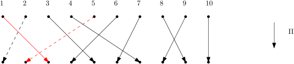
(a) For the permutation $\Pi$ depicted we have $J_{1}(\Pi)=5$. Indeed the set $W_{2}([5])=\{i:\{\Pi(i),\Pi(i)+1\}\subseteq\Pi[[5]]\}$ contains exactly $i=5$ (depicted by red lines) and $i=2$ (depicted by dashed lines), whereas $W_{2}([4])$ is empty.

(b) The permutation $\Pi_{J_{1}}=\operatorname{rk}(\Pi(1),\ldots,\Pi(5))$. We have $K_{1}(\Pi)=J_{1}(\Pi_{J_{1}})=3$ as witnessed by the red lines.

Figure 7.1: An illustration of $J_{1}$ and $K_{1}$

Recall that we have defined

$$w_{2}([j],\Pi_{n})\textbf{}\,=\,|\{i:\{\Pi_{n}(i),\Pi_{n}(i)+1\}\subseteq\Pi_{n}[[j]]\}|.$$ (194)

For a permutation $\pi$ and $M\in{\mathbb{N}}$ we define the function

$$J_{1}(\pi)=\inf\{j:w_{2}([j],\pi)\geq 1\},$$ (195)

where we agree as usual that the infimum of the empty set equals $\infty$. We also define

$$K_{1}=J_{1}\left(\Pi_{J_{1}(\Pi_{n})}\right),$$ (196)

where $\Pi_{J_{1}(\Pi_{n})}=\operatorname{rk}(\Pi_{n}(1),\ldots,\Pi_{n}(J_{1}(\Pi_{n}))$. See Figure 7.1 for an illustration of these definitions. We should note that $K_{1}$ is technically not always defined, indeed $J_{1}(\Pi_{n})$ may exceed $n$. However, if $\pi\in S_{n}$ with $n\geq 2$ then $w_{2}([1],\pi)=0$ and $w_{2}([n],\pi)\geq 1$ so that $J_{1}(\pi)\in\{2,\ldots,n\}$ and $K_{1}$ is finite for all such $\pi$.

Lemma 7.9.

Let $\alpha=\alpha(n)$ satisfy $|\alpha|\leq c/n$ for some constant $c>0$. Let $q=1-\alpha$, $\Pi_{n}\sim\operatorname{Mallows}(n,q)$ and $1\leq j\leq n$. Then for every $\varepsilon>0$ there exist $0<b_{1}<b_{2}$, depending on $\varepsilon$ and $c$, such that

$${\mathbb{P}}\left(b_{1}\sqrt{n}\leq J_{1}(\Pi_{n})\leq b_{2}\sqrt{n}\right)>1-\varepsilon,$$ (197)

provided that $n\geq n_{0}$ for some $n_{0}$ depending on $\varepsilon$ and $c$.

Proof.

Corollary 7.7 says that ${\mathbb{E}}w_{2}([j],\Pi_{n})\leq c_{U}^{2}j^{2}/n$. Setting $b_{1}=\sqrt{{\varepsilon}/{2c_{U}^{2}}}$, Markov’s inequality yields

$${\mathbb{P}}\left(J_{1}(\Pi_{n})\leq\left\lfloor b_{1}\sqrt{n}\right\rfloor\right)={\mathbb{P}}\left(w_{2}([\left\lfloor b_{1}\sqrt{n}\right\rfloor],\Pi_{n})\geq 1\right)\leq\frac{c_{U}^{2}(\left\lfloor b_{1}\sqrt{n}\right\rfloor)^{2}}{n}\leq\frac{\varepsilon}{2}.$$ (198)

For the other bound we will again use the fact that $w_{2}([j],\Pi_{n})\hskip 0.86108pt\raisebox{-0.43057pt}{$=$}\raisebox{4.30554pt}{{$\scriptstyle d$}}\hskip 3.44444ptY_{1}(j,\Pi_{n})+\ldots+Y_{n-1}(j,\Pi_{n})$. We claim that if $A_{m}<j/3$ and $Z_{m},Z_{m+1}\leq j/2$, then $Y_{m}(j,\Pi_{n})=\mathbf{1}_{\{\Pi_{n}(m),\Pi_{n}(m+1)\leq j\}}=1$. To see this, note that $A_{m}<j/3$ means that

$$\left|[j]\setminus\{\Pi_{n}(1),\ldots,\Pi_{n}(m)\}\right|\geq\left\lceil\frac{2j}{3}\right\rceil.$$ (199)

In this case, if $Z_{m}\leq j/2$ then $\Pi_{n}(m)\leq\lfloor\frac{j}{3}\rfloor+\lfloor\frac{j}{2}\rfloor<j$ and if additionally $Z_{m+1}\leq\frac{j}{2}$ then $\Pi_{n}(m+1)\leq\lfloor\frac{j}{3}\rfloor+\lfloor\frac{j}{2}\rfloor+1\leq j$.

So let $X_{i}$ be the indicator random variable for the event $\{Z_{i},Z_{i+1}\leq\frac{j}{2}\}$. If $A_{m}\leq j/3$ holds then $Y_{1}+\ldots+Y_{m}\geq X_{1}+\ldots+X_{m}$. Let $m\coloneqq\left\lfloor\gamma n\right\rfloor-1$ with $\gamma=\gamma(c)$ as in Lemma 7.8. Let $E$ be the set of even numbers in $[m]$ and $O$ be the set of odd numbers in $[m]$. For $n$ large enough, depending on $c$, we have $m/3<|E|,|O|<2m/3$. Moreover, the $X_{i}$ for $i\in E$ are mutually independent, as are the $X_{i}$ for $i\in O$. By Lemma 7.4 we also have

$$\mu_{E}\coloneqq{\mathbb{E}}\left(\sum_{i\in E}X_{i}\right)\geq|E|c_{L}^{2}\frac{j^{2}}{4n^{2}}\geq mc_{L}^{2}\frac{j^{2}}{12n^{2}},$$ (200)

and the same bound for $\mu_{O}\coloneqq{\mathbb{E}}\left(\sum_{i\in O}X_{i}\right)$. By Chernoff’s bound (Theorem 3.1 with $\varepsilon=\frac{1}{2}$) we have

$${\mathbb{P}}\left(\sum_{i\in E}X_{i}\leq mc_{L}^{2}\frac{j^{2}}{24n^{2}}\right)\leq{\mathbb{P}}\left(\sum_{i\in E}X_{i}\leq\frac{\mu_{E}}{2}\right)\leq\exp\left(-\frac{\mu_{E}}{8}\right)\leq\exp\left(-mc_{L}^{2}\frac{j^{2}}{96n^{2}}\right).$$ (201)

We have the same bound replacing $E$ by $O$ in the sums in (201), as we only used the bounds on $|E|$ and the mutual independence of $X_{i}$ for $i\in E$. Let $b_{2}$ be for the moment undetermined and set $j=\left\lfloor b_{2}\sqrt{n}\right\rfloor$. Then

$$\frac{mj^{2}}{n^{2}}\geq\frac{(\gamma n-1)(b_{2}\sqrt{n}-1)^{2}}{n^{2}}=(1+o(1))\frac{\gamma b_{2}^{2}n^{2}}{n^{2}}.$$ (202)

So we can select $b_{2}$ so large that $mc_{L}^{2}\frac{j^{2}}{24n^{2}}>1$ and such that the right–hand side of (201) is less than $\varepsilon/8$. By $[m]=E\uplus O$ we have

$${\mathbb{P}}\left(w_{2}([\left\lfloor b_{2}\sqrt{n}\right\rfloor],\Pi_{n})\leq 1\,|\,A_{m}\leq\frac{j}{3}\right) \leq{\mathbb{P}}\left(\sum_{i\in[m]}X_{i}\leq 1\,|\,A_{m}\leq\frac{j}{3}\right)\leq\frac{\varepsilon}{4\,{\mathbb{P}}\left(A_{m}\leq\frac{j}{3}\right)}.$$ (203)

By Lemma 7.8 and our choice of $m$ we have

$${\mathbb{P}}\left(w_{2}([\left\lfloor b_{2}\sqrt{n}\right\rfloor],\Pi_{n})\leq 1\right)\leq\frac{\varepsilon}{4}+e^{-Kj}=\frac{\varepsilon}{4}+e^{-K\left\lfloor b_{2}\sqrt{n}\right\rfloor},$$ (204)

where $K=K(c)$. For $n$ large enough, depending on $\varepsilon$ and $c$, this is at most $\varepsilon/2$. We note that ${\mathbb{P}}\left(J_{1}>\left\lfloor b_{2}\sqrt{n}\right\rfloor\right)$ only if $w_{2}([\left\lfloor b_{2}\sqrt{n}\right\rfloor],\Pi_{n})=0$, giving the desired bound. ∎

We now have an appropriate probabilistic bound on $J_{1}$ that we wist to extend to $K_{1}$. However, we cannot simply examine the permutation $\Pi_{J_{1}}$, as exposing the value of $J_{1}$ imposes some constraints on $\Pi_{J_{1}}$ so that the latter is no longer necessarily distributed as a Mallows permutation. The next lemma will show that $J_{1}(\Pi_{x})$ is monotonically increasing in $x$. Now, without exposing $J_{1}$ we have $J_{1}(\Pi_{\left\lfloor b_{1}\sqrt{n}\right\rfloor})=\Theta(n^{-1/4})$ and $J_{1}(\Pi_{\left\lceil b_{2}\sqrt{n}\right\rceil})=\Theta(n^{-1/4})$ with probability at least $1-2\varepsilon$. By the mentioned monotonicity of $J_{1}(\Pi_{x})$ we can thus sandwich $K_{1}$ within these bounds with probability at least $1-3\varepsilon$ by the previous lemma. The next two lemmas provide all details.

Lemma 7.10.

For every $n\geq 3$, $2\leq k\leq n-1$ and every $\pi\in S_{n}$ we have

$$J_{1}(\pi_{k})\leq J_{1}(\pi_{k+1}),$$ (205)

where $\pi_{k}=\operatorname{rk}(\pi(1),\ldots,\pi(k))$ and $\pi_{k+1}=\operatorname{rk}(\pi(1),\ldots,\pi(k+1))$.

Proof.

As $J_{1}(\pi_{k})\leq k$, we need only consider the case $J_{1}(\pi_{k+1})=a<k$. Then $w_{2}([a],\pi_{k+1})\geq 1$ so there is some $i\in[k+1]$ such that $\pi_{k+1}(i)$ and $\pi_{k+1}(i)+1$ are both contained in $\pi_{k+1}[[a]]$. This implies that $i\in[a]\subseteq[k-1]$ and $\pi_{k+1}(i)+1=\pi_{k+1}(a_{0})$ for some $a_{0}\in[a]$, which in turn implies $\mathbf{1}_{\{\pi(k+1)<\pi(i)\}}=\mathbf{1}_{\{\pi(k+1)<\pi(a_{0})\}}$. Thus

$$\pi_{k}(i)+1=\pi_{k+1}(i)+1-\mathbf{1}_{\{\pi(k+1)<\pi(i)\}}=\pi_{k+1}(a_{0})-\mathbf{1}_{\{\pi(k+1)<\pi(a_{0})\}}=\pi_{k}(a_{0}).$$ (206)

Thus $\pi_{k}(i)\in\pi_{k}[[a]]$ and $\pi_{k}(i)+1=\pi_{k}(a_{0})\in\pi_{k}[[a]]$. So $J_{1}(\pi_{k})\leq a$. ∎

Lemma 7.11.

Let $\alpha=\alpha(n)$ satisfy $|\alpha|\leq c/n$ for some constant $c>0$. Let $q=1-\alpha$ and $\Pi_{n}\sim\operatorname{Mallows}(n,q)$. Then for every $\varepsilon>0$ there exist positive constants $b_{1}^{\prime},b_{2}^{\prime}$ such that

$${\mathbb{P}}\left(b_{1}^{\prime}n^{1/4}\leq K_{1}(\Pi_{n})\leq b_{2}^{\prime}n^{1/4}\right)>1-\varepsilon,$$ (207)

provided that $n\geq n_{0}$ for some $n_{0}$ depending on $\varepsilon$ and $c$.

Proof.

By Lemma 7.9 there exists $0<b_{1}<b_{2}$ depending on $\varepsilon$ and $c$ such that

$${\mathbb{P}}\left(b_{1}\sqrt{n}\leq J_{1}(\Pi_{n})\leq b_{2}\sqrt{n}\right)\geq 1-\frac{\varepsilon}{3}.$$ (208)

Denote the event above by $E$. Define $k_{1}=\left\lfloor b_{1}\sqrt{n}\right\rfloor$, $k_{2}=\left\lceil b_{2}\sqrt{n}\right\rceil$ and $\Pi_{k_{1}}=\operatorname{rk}(\Pi_{n}(1),\ldots,\Pi_{n}(k_{1}))$ and similarly $\Pi_{k_{2}}$. Conditional on $E$, by $k_{1}\leq k_{2}$ and Lemma 7.10 we have

$$J_{1}(\Pi_{k_{1}})\leq K_{1}(\Pi_{n})\leq J_{1}(\Pi_{k_{2}}).$$ (209)

By Lemma 3.10 we have $\Pi_{k_{1}}\sim\operatorname{Mallows}(k_{1},q)$ where

$$|1-q|\leq\frac{c}{n}\leq\frac{cb_{1}}{k_{1}^{2}}.$$ (210)

Similarly $\Pi_{k_{2}}\sim\operatorname{Mallows}(k_{2},q)$ with $|1-q|\leq cb_{2}/k_{2}^{2}$. Lemma 7.9 says that there are $b_{1}^{\prime\prime},b_{2}^{\prime\prime}$ depending on $\varepsilon$ and $c$ (and on $b_{1}$ and $b_{2}$ which themselves depend on $\varepsilon$ and $c$) such that

$${\mathbb{P}}\left(b_{1}^{\prime\prime}\sqrt{k_{1}}\leq J_{1}(\Pi_{k_{1}})\right) \geq 1-\frac{\varepsilon}{3},$$ (211)

$${\mathbb{P}}\left(b_{2}^{\prime\prime}\sqrt{k_{2}}\geq J_{1}(\Pi_{k_{2}})\right) \geq 1-\frac{\varepsilon}{3},$$ (212)

provided that $k_{1}$ and $k_{2}$ both exceed some lower bound depending on $\varepsilon$ and $c$. These bounds together with (209) and ${\mathbb{P}}\left(E\right)>1-\varepsilon/3$ give

$${\mathbb{P}}\left(b_{1}^{\prime\prime}\sqrt{b_{1}}n^{1/4}\leq K_{1}(\Pi_{n})\leq b_{2}^{\prime\prime}\sqrt{b_{2}}n^{1/4}\right)\geq 1-\varepsilon.$$ (213)

∎

Lemma 7.12.

There exists a $\operatorname{\mathsf{TOTO}}$ formula $\psi$ such that the following holds: Let $\alpha=\alpha(n)$ satisfy $|\alpha|\leq c/n$ for some constant $c>0$, and $\Pi_{n}\sim\operatorname{Mallows}(n,1-\alpha)$. Then for every $\varepsilon>0$ there exist positive constants $b_{1}^{\prime},b_{2}^{\prime}$ such that with probability at least $1-\varepsilon$, there is a unique $j$ such that $\Pi_{n}\models\psi[j]$, and this unique $j$ satisfies the bounds

$$b_{1}^{\prime}n^{1/4}\leq j\leq b_{2}^{\prime}n^{1/4},$$ (214)

provided that $n\geq n_{0}$ for some $n_{0}$ depending on $\varepsilon$ and $c$.

Proof.

We have already found a formula that determines whether $i\in W_{2}([j],\Pi_{n})$ in (116), call this formula $\zeta(i,j)$. Then ${J}_{1}=j_{1}\in[n]$ if and only if $\Pi_{n}\models\xi[j_{1}]$ where

$$\xi(x)\coloneqq\exists z(\zeta(z,x))\wedge\forall w\left(w<_{1}x\rightarrow\neg\exists z\left(\zeta(z,w)\right)\right).$$ (215)

We now define the formula

$$\psi(x)\coloneqq\exists z\left(\xi(z)\wedge(x\leq_{1}z)\wedge\xi^{\leq}(z,x)\right),$$ (216)

where $\xi^{\leq}$ is the relativization of $\xi$, see Lemma 3.24. By Lemma 3.26, $K_{1}=j\in[n]$ if and only if $\Pi_{n}\models\psi[j]$, and such a unique $j$ always exists (as long as $n\geq 2$). By Lemma 7.11 there are $b_{1}^{\prime},b_{2}^{\prime}$ depending on $\varepsilon$ and $c$ such that this $j$ also satisfies (214) with probability at least $1-\varepsilon$. ∎

Proposition 7.13.

Let $\alpha=\alpha(n)$ satisfy $|\alpha|\leq c/n$ for some constant $c>0$. Let $q=1-\alpha$ and $\Pi_{n}\sim\operatorname{Mallows}(n,q)$. Then there is a sentence $\omega\in\operatorname{\mathsf{TOTO}}$ such that for all $n$ satisfying $W^{(2)}(\log^{**}\log^{**}n-1)<\log^{*}n$ we have

$${\mathbb{P}}(\Pi_{n}\models\omega)=\begin{cases}>\frac{9}{10}-O(n^{-1/4})&\text{if }\log^{**}\log^{**}n\text{ is even},\\ <\frac{1}{10}+O(n^{-1/4})&\text{if }\log^{**}\log^{**}n\text{ is odd},\end{cases}$$ (217)

where the implicit constants in the $O(n^{-1/4})$ terms depend on $c$.

Proof.

Let $\psi$ be as in Lemma 7.12 and let $\varphi$ be the sentence provided by Proposition 7.1. We define the sentence

$$\omega\coloneqq\exists z\left(\psi(z)\wedge\varphi^{\leq}(z)\right),$$ (218)

where $\varphi^{\leq}$ is the relativization of $\varphi$ as in Lemma 3.24.

Set $\varepsilon=\frac{1}{10}$. Let $0<b_{1}^{\prime}<b_{2}^{\prime}$, both depending on $c$, be as in Lemma 7.12. Let $E$ be the event that there is a unique $j$ such that $\Pi_{n}\models\psi[j]$ and that this unique $j$ satisfies (214). We have ${\mathbb{P}}\left(E\right)>\frac{9}{10}$ by Lemma 7.12. Letting $\Pi_{j}=\operatorname{rk}(\Pi_{n}(1),\ldots,\Pi_{n}(j))$ if $E$ holds, we have by Lemma 3.26 that

$${\mathbb{P}}\left(\Pi_{n}\models\omega\right) \geq\frac{9}{10}\cdot{\mathbb{P}}\left(\Pi_{j}\models\varphi\,|\,E\right),$$ (219)

$${\mathbb{P}}\left(\Pi_{n}\not\models\omega\right) \geq\frac{9}{10}\cdot{\mathbb{P}}\left(\Pi_{j}\not\models\varphi\,|\,E\right).$$ (220)

We will first show that conditional on $E$, the condition $W^{(2)}(\log^{**}\log^{**}n-1)<\log^{*}n$ implies that $\log^{**}\log^{**}n=\log^{**}\log^{**}j$ and $W^{(2)}(\log^{**}\log^{**}j-1)<\log\log j$, at least for $n$ larger than some lower bound depending on $b_{1}^{\prime}$ and $b_{2}^{\prime}$. Note that $W^{(2)}(\log^{**}\log^{**}n-1)<\log^{*}n$ implies

$$\log^{**}\log^{**}n-1<\log^{**}\log^{**}\log^{*}n\leq\log^{**}\log^{**}n.$$ (221)

This forces the second inequality to be an equality. If $n\geq j\geq b_{1}^{\prime}n^{1/4}>\log^{*}n$, then conditional on $E$ we indeed have that $\log^{**}\log^{**}j=\log^{**}\log^{**}n$. For $n$ exceeding some lower bound depending on $b^{\prime}_{1}$, we also have $\log^{*}n<\log\log b_{1}^{\prime}n^{1/4}$, so that in this case the event $E$ implies

$$W^{(2)}(\log^{**}\log^{**}n-1)=W^{(2)}(\log^{**}\log^{**}j-1)<\log^{*}n<\log\log b_{1}^{\prime}n^{1/4}\leq\log\log j.$$ (222)

Consider then the case $\log^{**}\log^{**}n$ even and let $\ell\coloneqq\left\lceil b_{1}^{\prime}n^{1/4}\right\rceil$ and $u\coloneqq\left\lfloor b_{2}^{\prime}n^{1/4}\right\rfloor$. For every $\ell\leq m\leq u$ we have $\Pi_{m}\coloneqq\operatorname{rk}(\Pi_{n}(1),\ldots,\Pi_{n}(m))\sim\operatorname{Mallows}(m,q)$, where

$$|1-q|\leq\frac{c}{n}\leq\frac{cb_{2}^{\prime 4}}{m^{4}}.$$ (223)

Thus, Proposition 7.1 yields

$${\mathbb{P}}\left(\Pi_{j}\models\varphi\,|\,E\right)\geq{\mathbb{P}}\left(\bigwedge\limits_{m=\ell}^{u}\Pi_{m}\models\varphi\right)\geq 1-\sum\limits_{m=\ell}^{u}{\mathbb{P}}\left(\Pi_{m}\not\models\varphi\right)\geq 1-u\,O(cb_{2}^{\prime 4}\ell^{-2}).$$ (224)

We conclude that

$${\mathbb{P}}\left(\Pi_{n}\models\omega\right)\geq\frac{9}{10}-O(n^{-1/4}).$$ (225)

We consider now the case $\log^{**}\log^{**}n$ odd. Again, conditioning on $E$, we are in the second case of Proposition 7.1 for $n$ large enough. We again have ${\mathbb{P}}\left(\Pi_{n}\not\models\omega\right)\geq\frac{9}{10}\,{\mathbb{P}}\left(\Pi_{j}\not\models\varphi\,|\,E\right)$. The same calculations as in (224) show that in this case ${\mathbb{P}}\left(\Pi_{n}\not\models\omega\right)>\frac{9}{10}-O(n^{-1/4})$. ∎

7.3 Lifting to $|1-q|<1/\log^{*}n$

In the section we finalize the proof of Theorem 1.2 Part (ii) by extending the results of the previous sections to $1-\frac{1}{\log^{*}n}<q<1+\frac{1}{\log^{*}n}$. We will proceed as follows: We partition the interval $(1-\frac{1}{\log^{*}n},1+\frac{1}{\log^{*}n})$ into the parts

$${\mathcal{D}}_{1}\coloneqq\left(1-\frac{1}{\log^{*}n},1-\frac{c}{n}\right),\ \ {\mathcal{D}}_{2}\coloneqq\left[1-\frac{c}{n},1+\frac{c}{n}\right],\ \ {\mathcal{D}}_{3}\coloneqq\left(1+\frac{c}{n},1+\frac{1}{\log^{*}n}\right).$$ (226)

With foresight we set $c=50$. We will find $\operatorname{\mathsf{TOTO}}$ sentences $\rho,\xi_{1}$ and $\xi_{2}$ and disjoint infinite sets $A^{-},A^{+}\subsetneq{\mathbb{N}}$ such that all bounds in Table 1 hold. Before we show the existence of such sentences with the desired properties, we show how they imply Theorem 1.2 Part (ii).

		$1-\frac{1}{\log^{*}n}<q<1-\frac{50}{n}$	$|1-q|\leq\frac{50}{n}$	$1+\frac{50}{n}<q<1+\frac{1}{\log^{*}n}$
$n>50$	${\mathbb{P}}(\Pi_{n}\models\rho)$	$\leq 0.1$		$\geq 0.9$
$n\in A^{+}$	${\mathbb{P}}(\Pi_{n}\models\xi_{1})$	$\geq 0.8$	$\geq 0.8$
	${\mathbb{P}}(\Pi_{n}\models\xi_{2})$		$\geq 0.8$	$\geq 0.8$
$n\in A^{-}$	${\mathbb{P}}(\Pi_{n}\models\xi_{1})$	$\leq 0.2$	$\leq 0.2$
	${\mathbb{P}}(\Pi_{n}\models\xi_{2})$		$\leq 0.2$	$\leq 0.2$

Table 1: We find $\operatorname{\mathsf{TOTO}}$ sentences $\rho,\xi_{1}$ and $\xi_{2}$ and two disjoint infinite set $A^{-},A^{+}\subsetneq{\mathbb{N}}$ such that the probability that $\Pi_{n}\sim\operatorname{Mallows}(n,q)$ satisfies each of the sentences is as shown.

Proof of Theorem 1.2 Part (ii).

We may assume that $A^{-}$ and $A^{+}$ contain only numbers exceeding $50$, so that the bounds on ${\mathbb{P}}\left(\Pi_{n}\models\rho\right)$ in Table 1 hold for all $n\in A^{-}\uplus A^{+}$. Let

$$\varphi\coloneqq\left(\rho\rightarrow\xi_{2}\right)\wedge((\neg\rho)\rightarrow\xi_{1}).$$ (227)

As $\Pi_{n}$ satisfies exactly one of $\rho$ and $\neg\rho$, any of the three events

$$E_{1}\coloneqq\{\Pi_{n}\models(\neg\rho)\wedge\xi_{1}\},\quad E_{2}\coloneqq\{\Pi_{n}\models(\xi_{1}\wedge\xi_{2})\}\quad\text{or}\quad E_{3}\coloneqq\{\Pi_{n}\models\rho\wedge\xi_{2}\}$$ (228)

imply that $\Pi_{n}\models\varphi$. For $n\in A^{+}$, by the bounds in Table 1 we have that

$$\text{if }\quad q\in{\mathcal{D}}_{1}\quad\text{then}\quad{\mathbb{P}}\left(E_{1}\right) \geq 1-0.1-0.2=0.7,$$ (229)

$$\text{if }\quad q\in{\mathcal{D}}_{2}\quad\text{then}\quad{\mathbb{P}}\left(E_{2}\right) \geq 1-0.2-0.2=0.6,$$ (230)

$$\text{if }\quad q\in{\mathcal{D}}_{3}\quad\text{then}\quad{\mathbb{P}}\left(E_{3}\right) \geq 1-0.1-0.2=0.7.$$ (231)

In general, for $n\in A^{+}$ and $q\in(1-\frac{1}{\log^{*}n},1+\frac{1}{\log^{*}n})={\mathcal{D}}_{1}\uplus{\mathcal{D}}_{2}\uplus{\mathcal{D}}_{3}$ we have ${\mathbb{P}}\left(\Pi_{n}\models\varphi\right)\geq 0.6$.

We now consider $n\in A^{-}$. Note that the three events

$$F_{1}\coloneqq\{\Pi_{n}\not\models\rho\wedge\Pi_{n}\not\models\xi_{1}\},\quad F_{2}\coloneqq\{\Pi_{n}\not\models(\xi_{1}\vee\xi_{2})\}\quad\text{and}\quad F_{3}\coloneqq\{\Pi_{n}\models\rho\wedge\Pi_{n}\not\models\xi_{2}\}$$ (232)

now each imply that $\Pi_{n}\not\models\varphi$. For $n\in A^{-}$ the bounds in Table 1 now give that

$$\text{if }\quad q\in{\mathcal{D}}_{1}\quad\text{then}\quad{\mathbb{P}}\left(F_{1}\right) \geq 1-0.1-0.2=0.7,$$ (233)

$$\text{if }\quad q\in{\mathcal{D}}_{2}\quad\text{then}\quad{\mathbb{P}}\left(F_{2}\right) \geq 1-0.2-0.2=0.6,$$ (234)

$$\text{if }\quad q\in{\mathcal{D}}_{3}\quad\text{then}\quad{\mathbb{P}}\left(F_{3}\right) \geq 1-0.1-0.2=0.7.$$ (235)

So for $n\in A^{-}$ and $q\in(1-1/\log^{*}n,1+1/\log^{*}n)$ we have ${\mathbb{P}}\left(\Pi_{n}\not\models\varphi\right)\geq 0.6$.

As both $A^{-}$ and $A^{+}$ have infinite cardinality, we conclude that ${\mathbb{P}}\left(\Pi_{n}\models\varphi\right)$ does not have a limit as $n\to\infty$ for any sequence $q=q(n)$ satisfying $1-1/\log^{*}n<q<1+1/\log^{*}n$. ∎

So it remains to find $\rho,\xi_{1},\xi_{2},A^{-}$ and $A^{+}$ and prove the bounds in Table 1. We start by defining the $\operatorname{\mathsf{TOTO}}$ sentence $\rho$ as

$$\rho=\exists xy\left(\neg\exists w(\mathsf{succ}_{1}(w,x)\vee\mathsf{succ}_{1}(y,w))\wedge(y<_{2}x)\right).$$ (236)

If $n\geq 1$, then there always exist unique $x$ and $y$ such that $\neg\exists w(\mathsf{succ}_{1}(w,x)\vee\mathsf{succ}_{1}(y,w))$, namely $x=1$ and $y=n$ the largest element in $[n]$. Then $\Pi_{n}\models\rho$ precisely when $\Pi_{n}(1)>\Pi_{n}(n)$.

Lemma 7.14.

Let $\Pi_{n}\sim\operatorname{Mallows}(n,q)$. For every $n>50$ we have

$${\mathbb{P}}\left(\Pi_{n}\not\models\rho\right) \geq 0.9\qquad\text{ if }q<1-\frac{50}{n},$$ (237)

$${\mathbb{P}}\left(\Pi_{n}\models\rho\right) \geq 0.9\qquad\text{ if }q>1+\frac{50}{n}.$$ (238)

Proof.

Recall once more the definition of $\operatorname{TruncGeo}(n,p)$ random variables as in (11), valid for $p\in(-\infty,0)\cup(0,1)$.

We first consider the case $q>1+50/n$. Recall that we defined the mapping $r_{n}:[n]\to[n]$ by $r_{n}:i\to n-i+1$. By $r_{n}(1)=n$ we may estimate

$${\mathbb{P}}\left(\Pi_{n}(n)\geq\frac{n}{3}+1\right)={\mathbb{P}}\left((r_{n}\circ\Pi_{n}\circ r_{n})(1)\leq n-\frac{n}{3}\right)={\mathbb{P}}\left(\Pi_{n}(1)\leq\frac{2n}{3}\right),$$ (239)

where we used the fact that $r_{n}\circ\Pi_{n}\circ r_{n}\hskip 0.86108pt\raisebox{-0.43057pt}{$=$}\raisebox{4.30554pt}{{$\scriptstyle d$}}\hskip 3.44444pt\Pi_{n}$. Using this estimate we have

$${\mathbb{P}}\left(\Pi_{n}\models\rho\right)\geq{\mathbb{P}}\left(\Pi_{n}(1)>\frac{2n}{3}\text{ and }\Pi_{n}(n)<\frac{n}{3}+1\right)\geq 1-2\cdot{\mathbb{P}}\left(\Pi_{n}(1)\leq\frac{2n}{3}\right).$$ (240)

The value $\Pi_{n}(1)$ follows a $\operatorname{TruncGeo}(n,1-q)$ distribution, so that

$${\mathbb{P}}\left(\Pi_{n}\models\rho\right) >1-2\cdot\frac{q-1}{q^{n}-1}\sum\limits_{i=0}^{\left\lfloor 2n/3\right\rfloor}q^{i}$$ (241)

$$=1-2\cdot\frac{q^{\left\lfloor 2n/3\right\rfloor+1}-1}{q^{n}-1}$$ (242)

$$>1-2\cdot\frac{q^{3n/4}-1}{q^{n}-1}.$$ (243)

The last inequality holds as $n>50$ implies that $\left\lfloor 2n/3\right\rfloor+1<3n/4$. Now, for all $1<x<y$ it holds that $\frac{x-1}{y-1}<\frac{x}{y}$, so that $1<q<q^{n}$ implies

$${\mathbb{P}}\left(\Pi_{n}\models\rho\right)>1-2q^{-n/4}>1-2\left(1+\frac{50}{n}\right)^{-n/4}.$$ (244)

By $n>50$, the latter quantity is at least $1-2\cdot 2^{-n/4}>1-2\cdot 2^{-12.5}>0.9$.

Now suppose that $q<1-50/n$ and that $n>50$. Then

$$\frac{1}{q}>\frac{1}{1-\frac{50}{n}}=\sum_{i\geq 0}\left(\frac{50}{n}\right)^{i}>1+\frac{50}{n}.$$ (245)

Recalling that for $\Pi_{n}\sim\operatorname{Mallows}(n,q)$ we have $r_{n}\circ\Pi_{n}\hskip 0.86108pt\raisebox{-0.43057pt}{$=$}\raisebox{4.30554pt}{{$\scriptstyle d$}}\hskip 3.44444pt\operatorname{Mallows}(n,1/q)$ gives

$${\mathbb{P}}\left(\Pi_{n}\not\models\rho\right)={\mathbb{P}}\left(r_{n}\circ\Pi_{n}\models\rho\right)>0.9.$$ (246)

∎

We now build up a collection of results that will allow us to find $\xi_{1}$ and $\xi_{2}$ with the desired properties. For the next few lemmas we will consider $c=100$ instead of $50$ to simplify some of the manipulations later on.

Lemma 7.15.

Let $q=q(n)$ be such that $1-100/n\leq q\leq 1+100/n$. Then there exists an absolute constant $c_{1}>0$ such that for $\Pi_{n}\sim\operatorname{Mallows}(n,q)$ and $n\geq 400$ we have

$${\mathbb{P}}\left(c_{1}n\leq\Pi_{n}^{-1}(1)\right)>0.99.$$ (247)

Proof.

If $q=1$, then $\Pi_{n}\sim\operatorname{Mallows}(n,q)$ is uniformly distributed over $S_{n}$. Then $\Pi_{n}^{-1}(1)$ is uniformly distributed over $[n]$ and such $c_{1}$ clearly exists.

So let $q\neq 1$. As before, we note that $\Pi_{n}^{-1}\hskip 0.86108pt\raisebox{-0.43057pt}{$=$}\raisebox{4.30554pt}{{$\scriptstyle d$}}\hskip 3.44444pt\Pi_{n}$ so that also $\Pi_{n}^{-1}(1)\hskip 0.86108pt\raisebox{-0.43057pt}{$=$}\raisebox{4.30554pt}{{$\scriptstyle d$}}\hskip 3.44444pt\Pi_{n}(1)\hskip 0.86108pt\raisebox{-0.43057pt}{$=$}\raisebox{4.30554pt}{{$\scriptstyle d$}}\hskip 3.44444ptZ_{1}$ where ${Z_{1}\sim\operatorname{TruncGeo}(n,1-q)}$. By Lemma 7.4 there is a $c_{U}>0$ such that for $n\geq 400$ we have

$${\mathbb{P}}\left(Z_{1}<c_{1}n\right)\leq c_{U}\frac{\left\lfloor c_{1}n\right\rfloor}{n}.$$ (248)

For $c_{1}$ small enough this is less than $0.01$. ∎

Lemma 7.16.

There exist constants $0<c_{1}<c_{2}$ and $n_{0}$ such that for $n\geq n_{0}$ and any sequence $q=q(n)$ satisfying $1-1/\log^{*}n<q<1-100/n$, the random permutation $\Pi_{n}\sim\operatorname{Mallows}(n,q)$ satisfies

$${\mathbb{P}}\left(\frac{c_{1}}{1-q}\leq\Pi_{n}^{-1}(1)\leq\frac{c_{2}}{1-q}\right)>0.99.$$ (249)

Proof.

We again have $\Pi_{n}^{-1}(1)\hskip 0.86108pt\raisebox{-0.43057pt}{$=$}\raisebox{4.30554pt}{{$\scriptstyle d$}}\hskip 3.44444ptZ_{1}$ where ${Z_{1}\sim\operatorname{TruncGeo}(n,1-q)}$. Therefore the inequalities $q<1-100/n<e^{-100/n}<1$ imply that

$${\mathbb{P}}\left(\Pi_{n}^{-1}(1)<\frac{c_{1}}{1-q}\right)\leq\frac{1-q}{1-q^{n}}\sum\limits_{i=1}^{\left\lfloor\frac{c_{1}}{1-q}\right\rfloor}q^{i-1}<\frac{c_{1}}{1-q^{n}}<\frac{c_{1}}{1-e^{-100}}.$$ (250)

Clearly the above is less than $0.005$ for $c_{1}$ small enough.

For the remaining bound, Markov’s inequality gives

$${\mathbb{P}}\left(\Pi^{-1}(1)>\frac{c_{2}}{1-q}\right)={\mathbb{P}}\left(\Pi^{-1}(1)-1>\frac{c_{2}-1+q}{1-q}\right)\leq\frac{(1-q){\mathbb{E}}(\Pi_{n}^{-1}(1)-1)}{c_{2}-1+q}.$$ (251)

Theorem 3.15 implies that ${\mathbb{E}}(\Pi^{-1}_{n}(1)-1)\leq\min(\frac{2q}{1-q},n-1)\leq\frac{2}{1-q}$. So

$${\mathbb{P}}\left(\Pi^{-1}(1)>\frac{c_{2}}{1-q}\right)\leq\frac{2}{c_{2}-1+q}<\frac{2}{c_{2}-\frac{1}{\log^{*}n}}.$$ (252)

For $n$ and $c_{2}$ large enough the above is less than $0.005$, finishing the proof. ∎

We now combine the previous two lemmas into a form that will be convenient for us.

Lemma 7.17.

There exist absolute constants $n_{1},c_{1},c_{2}$ and a $\operatorname{\mathsf{TOTO}}$ formula $\lambda(y)$ with one free variable $y$ such that the following holds: For $1-1/\log^{*}n<q<1+100/n$ and $\Pi_{n}\sim\operatorname{Mallows}(n,q)$, if $n\geq n_{1}$, then

1. $\Pi_{n}\models\lambda[x]$ if and only if $\Pi_{n}(x+1)=1$;

2. $${\mathbb{P}}\left(\left\{\exists x\text{ s.t. }\Pi_{n}(x+1)=1\text{ and }x\geq c_{1}\log^{*}n\text{ and }|1-q|\leq\frac{c_{2}}{x}\right\}\right)\geq 0.99.$$ (253)

Proof.

Let $\lambda(y)$ be the formula

$$\lambda(y)\coloneqq\exists z\ (\mathsf{succ}_{1}(y,z)\wedge\neg\exists w\ (w<_{2}z)).$$ (254)

Then $\Pi_{n}\models\lambda[N]$ if and only if the successor under $<_{1}$ of $N$ is the smallest number under the ordering $<_{2}$, that is, if and only if $\Pi_{n}(N+1)=1$. So let $N=\Pi^{-1}_{n}(1)-1$.

We consider two cases. First suppose that $1-100/n\leq q\leq 1+100/n$. By Lemma 7.15 there is a $c_{1}$ such that for $n$ large enough we have $N\geq c_{1}n-1>c_{1}\log^{*}n$ with probability at least $0.99$. Moreover, by $N\leq n$ we have $|1-q|\leq 100/n\leq 100/N$. This finishes the first case.

Suppose then that $1-1/\log^{*}n<q<1-100/n$. By Lemma 7.16 there are absolute $c_{1},c_{2}$ such that with probability at least $0.99$ we have

$$\frac{c_{1}}{1-q}\leq N+1\leq\frac{c_{2}}{1-q}.$$ (255)

The first inequality gives $N\geq\frac{c_{1}}{1-q}-1>c_{1}\log^{*}n-1$. For $n$ large enough (depending on the absolute constant $c_{1}$) this is at least, say, $\frac{c_{1}}{2}\log^{*}n$. The second inequality gives $0<1-q\leq c_{2}/N$. This finishes the second case as well. ∎

We will need the following algebraic lemma before we can turn to the existence of $\xi_{1},\xi_{2}$ as advertised at the start of this section. Recall the definitions of $W(\cdot)$ and $T(\cdot)$ from Section 3.4.

Lemma 7.18.

Let $c_{1}$ be as given in Lemma 7.17. Then there exists an $m\in{\mathbb{N}}$ such that the following holds: Let $t\geq m$, set $n\coloneqq W^{(2)}(t)$ and let $N$ satisfy $c_{1}\log^{*}n\leq N\leq n$. Then

$$W^{(2)}(\log^{**}\log^{**}N-1)<\log^{*}N,$$ (256)

and

$$\log^{**}\log^{**}N=t.$$ (257)

Proof.

First, let $m>3$ so that by Lemma 3.29 the inequality

$$T^{(3)}\circ W^{(2)}(t-1)<W^{(2)}(t)$$ (258)

holds for all $t\geq m$. We may also select $m$ so large that for all $t\geq m$

$$c_{1}\,T^{(2)}\circ W^{(2)}(t-1)>T\circ W^{(2)}(t-1).$$ (259)

We claim that any $m$ satisfying these two conditions is as desired. To see this, let $t\geq m$, $n=W^{(2)}(t)$ and $c_{1}\log^{*}n\leq N\leq n$. The inequalities (259) and (258) imply that

$$N\geq c_{1}\log^{*}W^{(2)}(t)>c_{1}\log^{*}(T^{(3)}\circ W^{(2)}(t-1))>T\circ W^{(2)}(t-1).$$ (260)

Thus

$$\log^{**}\log^{**}N \geq\log^{**}\log^{**}(T\circ W^{(2)}(t-1))>t-1.$$ (261)

As we trivially have $\log^{**}\log^{**}N\leq\log^{**}\log^{**}n=t$, we conclude that $\log^{**}\log^{**}N=t$. Moreover, (260) also implies that

$$\log^{*}N>W^{(2)}(t-1)=W^{(2)}(\log^{**}\log^{**}N-1).$$ (262)

∎

For what follows, we let $S_{0}$ be the set containing only the empty permutation; that is, the $\operatorname{\mathsf{TOTO}}$ structure with empty domain. We let $\operatorname{Mallows}(0,q)$ be the degenerate distribution with support $S_{0}$.

Lemma 7.19.

Let $0<q\leq 1$ and $\Pi_{n}\sim\operatorname{Mallows}(n,q)$. If $N:=\Pi_{n}^{-1}(1)-1$ and $\Pi_{N}:=\operatorname{rk}(\Pi_{n}(1),\dots,\Pi_{n}(N))$, then

$$\Pi_{N}\hskip 0.86108pt\raisebox{-0.43057pt}{$=$}\raisebox{4.30554pt}{{$\scriptstyle d$}}\hskip 3.44444pt\operatorname{Mallows}(N,q),$$ (263)

(I.e.,  we generate a Mallows distribution with $n$ random.)

Proof.

Let $0\leq m<n$ and $\pi\in S_{m}$, we will determine the distribution of $\Pi_{N}$ conditional on $N=m$. If $m=0$, then we trivially have $\Pi_{m}\sim\operatorname{Mallows}(m,q)$, so we may consider $m\geq 1$. We have for each $\pi\in S_{m}$

$${\mathbb{P}}\left(\Pi_{m}=\pi\,|\,N=m\right)=\frac{{\mathbb{P}}\left(\Pi_{m}=\pi\text{ and }N=m\right)}{{\mathbb{P}}\left(N=m\right)}$$ (264)

If $N=m$, then $\Pi(m+1)=1$. So the two events $\{\Pi_{m}=\pi\}$ and $\{N=m\}$ imply that $(i,m)$ is an inversion of $\Pi_{m+1}$ for every $i\leq m$. That is, conditioning on these two events we have $\operatorname{inv}(\Pi_{m+1})=\operatorname{inv}(\pi)+m$. We obtain that

$${\mathbb{P}}\left(\Pi_{m}=\pi\,|\,N=m\right)=\frac{q^{\operatorname{inv}(\pi)}}{F(m,q)},$$ (265)

for some function $F(m,q)$. In fact, summing the above over all $\pi\in S_{m}$ gives one, so that $F(m,q)$ necessarily equals $\sum_{\pi\in S_{m}}q^{\operatorname{inv}(\pi)}$. ∎

We are now ready to show the existence of $\xi_{1}$ satisfying the bounds in Table 1.

Lemma 7.20.

There exists a sentence $\xi_{1}\in\operatorname{\mathsf{TOTO}}$ and two infinite disjoint sets $A^{+},A^{-}\subseteq{\mathbb{N}}_{>100}$ such that for

$$1-\frac{1}{\log^{*}n}\leq q<1+\frac{100}{n}$$ (266)

and $\Pi_{n}\sim\operatorname{Mallows}(n,q)$ we have

$${\mathbb{P}}\left(\Pi_{n}\models\xi_{1}\right) >0.8,\quad\text{if }\ n\in A^{+},$$ (267)

$${\mathbb{P}}\left(\Pi_{n}\models\xi_{1}\right) <0.2,\quad\text{if }\ n\in A^{-}.$$ (268)

Proof.

Let $n_{1},c_{1},c_{2}$ and $\lambda(y)$ be as provided by Lemma 7.17, and let the event $E$ be as in (253). Let $m$ be as given in Lemma 7.18. Without loss of generality, we may assume that $m$ is so large that $W^{(2)}(m)>n_{1}$. Define the $\operatorname{\mathsf{TOTO}}$ sentence $\xi_{1}$ as

$$\xi_{1}=\exists z(\lambda(z)\wedge\omega^{\leq}(z)),$$ (269)

where $\omega$ is the sentence $\omega(c_{1})$ as given in Proposition 7.13 (using the absolute constant $c_{1}$), and $\omega^{\leq}$ is its relativization as in Lemma 3.24. Then by Lemma 3.26

$${\mathbb{P}}\left(\Pi_{n}\models\xi_{1}\,|\,E\right)={\mathbb{P}}\left(\Pi_{N}\models\omega\,|\,E\right).$$ (270)

Let $t\geq m$ be even and set $n=W^{(2)}(t)$. Then for all $c_{1}\log^{*}n\leq N<n$ we have by Lemma 7.18 that $N$ satisfies the conditions of the first case in Proposition 7.13, so that Lemma 7.19 yields

$${\mathbb{P}}\left(\Pi_{N}\models\omega\,|\,E\right)>\frac{9}{10}-O\left((\log^{*}n)^{-1/4}\right).$$ (271)

For $n$ large enough (i.e., $t$ large enough), this is at least $0.81$. As ${\mathbb{P}}\left(E\right)>0.99$ we have that ${\mathbb{P}}\left(\Pi_{n}\models\xi_{1}\right)>0.8$.

Completely analogously, when $t$ is odd, then ${\mathbb{P}}\left(\Pi_{N}\models\omega\,|\,E\right)<0.19$. Using ${\mathbb{P}}\left(E\right)>0.99$ we again conclude that there are also infinitely many $n=W^{(2)}(t)$ with $t$ now odd, such that ${\mathbb{P}}\left(\Pi_{n}\models\xi_{1}\right)<0.2$. ∎

Remark 7.21.

As alluded to earlier, Lemma 7.20 is slightly stronger than needed: we only require the bounds for the smaller domain ${\mathbb{P}}\left(\Pi_{n}\models\xi_{1}\right)$ for $1-1/\log^{*}n<q<1+50/n$.

The last lemma of this section gives the existence of $\xi_{2}$ with the desired specifications, finishing the proof of Theorem 1.2 Part (ii).

Lemma 7.22.

Let $A^{-}$ and $A^{+}$ be as in Lemma 7.20. There exists a $\operatorname{\mathsf{TOTO}}$ sentence $\xi_{2}$ such that for

$$1-\frac{50}{n}\leq q<1+\frac{1}{\log^{*}n}$$ (272)

and $\Pi_{n}\sim\operatorname{Mallows}(n,q)$ we have

$${\mathbb{P}}\left(\Pi_{n}\models\xi_{2}\right) >0.8,\quad\text{if }\ n\in A^{+},$$ (273)

$${\mathbb{P}}\left(\Pi_{n}\models\xi_{2}\right) <0.2,\quad\text{if }\ n\in A^{-}.$$ (274)

Proof.

Let $\xi_{2}\coloneqq\xi_{1}^{\operatorname{reverse}}$, where $\xi_{1}$ is as provided by Lemma 7.20. Let $1-\frac{50}{n}\leq q<1+\frac{1}{\log^{*}n}$. Then

$$\frac{1}{q}\leq\frac{1}{1-\frac{50}{n}}=1+\frac{50}{n-50}.$$ (275)

If $n\geq 100$ then this is at most $1+100/n$, as is simple to verify. Moreover,

$$\frac{1}{q}>\frac{1}{1+\frac{1}{\log^{*}n}}=1-\frac{1}{\log^{*}n+1}>1-\frac{1}{\log^{*}n}.$$ (276)

Recall from Lemma 7.20 that $A^{-}$ and $A^{+}$ are subsets of ${\mathbb{N}}_{>100}$. By Lemma 3.27 and Lemma 7.20 we have for $\Pi_{n}\sim\operatorname{Mallows}(n,q)$ that

$${\mathbb{P}}\left(\Pi_{n}\models\xi_{2}\right)={\mathbb{P}}\left(r_{n}\circ\Pi_{n}\models\xi_{1}\right)=\begin{cases}>0.8&\text{if }n\in A^{+},\\ <0.2&\text{if }n\in A^{-}.\\ \end{cases}$$ (277)

∎

Acknowledgements

We thank Kevin Compton, Valentin Féray, Tomasz Łuczak, Marc Noy and Joel Spencer for helpful discussions and pointers to the literature.

References

- [1] L. Addario-Berry and B. Corsini. The height of Mallows trees. Ann. Probab., 49(5):2220–2271, 2021.
- [2] M. Albert, M. Bouvel, and V. Féray. Two first-order logics of permutations. J. Combin. Theory Ser. A, 171:105–158, 46, 2020.
- [3] M. Albert, M. Bouvel, V. Féray, and M. Noy. Convergence law for -avoiding permutations. arXiv preprint arXiv:2210.05537, 2022.
- [4] M. H. Albert and A. M. Frieze. Random graph orders. Order, 6(1):19–30, 1989.
- [5] O. Angel, A. E. Holroyd, T. Hutchcroft, and A. Levy. Mallows permutations as stable matchings. Canad. J. Math., 73(6):1531–1555, 2021.
- [6] R. Arratia and S. Tavaré. The cycle structure of random permutations. Ann. Probab., 20(3):1567–1591, 1992.
- [7] R. Basu and N. Bhatnagar. Limit theorems for longest monotone subsequences in random Mallows permutations. Ann. Inst. Henri Poincaré Probab. Stat., 53(4):1934–1951, 2017.
- [8] I. Benjamini, N. Berger, C. Hoffman, and E. Mossel. Mixing times of the biased card shuffling and the asymmetric exclusion process. Trans. Amer. Math. Soc., 357(8):3013–3029, 2005.
- [9] N. Bhatnagar and R. Peled. Lengths of monotone subsequences in a Mallows permutation. Probab. Theory Related Fields, 161(3-4):719–780, 2015.
- [10] B. Bollobás and P. Winkler. The longest chain among random points in euclidean space. Proceedings of the American Mathematical Society, 103(2):347–353, 1988.
- [11] A. Borodin, P. Diaconis, and J. Fulman. On adding a list of numbers (and other one-dependent determinantal processes). Bull. Amer. Math. Soc. (N.S.), 47(4):639–670, 2010.
- [12] S. Braunfeld and M. Kukla. Logical limit laws for layered permutations and related structures. arXiv preprint arXiv:2111.06307, 2021.
- [13] M. Braverman and E. Mossel. Sorting from noisy information. Preprint, available from http://arxiv.org/abs/0910.1191, 2009.
- [14] G. Brightwell. Models of random partial orders, volume 187. Cambridge University Press Cambridge, 1993.
- [15] G. Brightwell and M. Luczak. The mathematics of causal sets. In Recent Trends in Combinatorics, pages 339–365. Springer, 2016.
- [16] Kevin J. Compton. A logical approach to asymptotic combinatorics. II. Monadic second-order properties. J. Combin. Theory Ser. A, 50(1):110–131, 1989.
- [17] H. Crane and S. DeSalvo. Pattern avoidance for random permutations. Discrete Math. Theor. Comput. Sci., 19(2):Paper No. 13, 24, 2017.
- [18] H. Crane, S. DeSalvo, and S. Elizalde. The probability of avoiding consecutive patterns in the Mallows distribution. Random Structures Algorithms, 53(3):417–447, 2018.
- [19] P. Diaconis and A. Ram. Analysis of systematic scan Metropolis algorithms using Iwahori-Hecke algebra techniques. volume 48, pages 157–190. 2000. Dedicated to William Fulton on the occasion of his 60th birthday.
- [20] R. Douc, E. Moulines, P. Priouret, and P. Soulier. Markov chains. Springer Series in Operations Research and Financial Engineering. Springer, Cham, 2018.
- [21] J. Enright, K. Meeks, W. Pettersson, and J. Sylvester. Tangled paths: A random graph model from Mallows permutations. arXiv preprint arXiv:2108.04786, 2021.
- [22] C. Even-Zohar and C. Leng. Counting small permutation patterns. In Proceedings of the 2021 ACM-SIAM Symposium on Discrete Algorithms (SODA), pages 2288–2302. SIAM, 2021.
- [23] X. Fang, H. L. Gan, S. Holmes, H. Huang, E. Peköz, A. Röllin, and W. Tang. Arcsine laws for random walks generated from random permutations with applications to genomics. J. Appl. Probab., 58(4):851–867, 2021.
- [24] J. Foy and A. R. Woods. Probabilities of sentences about two linear orderings. In Feasible mathematics (Ithaca, NY, 1989), volume 9 of Progr. Comput. Sci. Appl. Logic, pages 181–193. Birkhäuser Boston, Boston, MA, 1990.
- [25] A. Gladkich and R. Peled. On the cycle structure of Mallows permutations. Ann. Probab., 46(2):1114–1169, 2018.
- [26] A. Gnedin and G. Olshanski. -exchangeability via quasi-invariance. Ann. Probab., 38(6):2103–2135, 2010.
- [27] A. Gnedin and G. Olshanski. The two-sided infinite extension of the Mallows model for random permutations. Adv. in Appl. Math., 48(5):615–639, 2012.
- [28] W. Gontcharoff. Sur la distribution des cycles dans les permutations. C. R. (Doklady) Acad. Sci. URSS (N.S.), 35:267–269, 1942.
- [29] R. L. Goodstein. Transfinite ordinals in recursive number theory. J. Symbolic Logic, 12:123–129, 1947.
- [30] G. R. Grimmett and D. R. Stirzaker. Probability and random processes. Oxford University Press, New York, third edition, 2001.
- [31] S. Haber and M. Krivelevich. The logic of random regular graphs. Journal of combinatorics, 1(4):389–440, 2010.
- [32] J. He. A central limit theorem for descents of a Mallows permutation and its inverse. Ann. Inst. Henri Poincaré Probab. Stat., 58(2):667–694, 2022.
- [33] J. He, T. Müller, and T. W. Verstraaten. Cycles in Mallows random permutations. Preprint, available from https://arxiv.org/abs/2201.11610, 2022.
- [34] P. Heinig, T. Müller, M. Noy, and A. Taraz. Logical limit laws for minor-closed classes of graphs. Journal of Combinatorial Theory, Series B, 130:158–206, 2018.
- [35] W. Hodges. A shorter model theory. Cambridge University Press, Cambridge, 1997.
- [36] A. E. Holroyd, T. Hutchcroft, and A. Levy. Mallows permutations and finite dependence. Ann. Probab., 48(1):343–379, 2020.
- [37] N. Immerman. Descriptive complexity. Graduate Texts in Computer Science. Springer-Verlag, New York, 1999.
- [38] S. Janson, T. Łuczak, and A. Rucinski. Random graphs. Wiley-Interscience Series in Discrete Mathematics and Optimization. Wiley-Interscience, New York, 2000.
- [39] K. Jin. The length of the longest common subsequence of two independent Mallows permutations. Ann. Appl. Probab., 29(3):1311–1355, 2019.
- [40] D. E. Knuth. Mathematics and computer science: Coping with finiteness. Science, 194(4271):1235–1242, 1976.
- [41] V. F. Kolchin. A problem of the allocation of particles in cells and cycles of random permutations. Theory of Probability & Its Applications, 16(1):74–90, 1971.
- [42] V. Koponen. Random graphs with bounded maximum degree: asymptotic structure and a logical limit law. Discrete Mathematics & Theoretical Computer Science, 14, 2012.
- [43] D. Král and O. Pikhurko. Quasirandom permutations are characterized by 4-point densities. Geometric and Functional Analysis, 23(2):570–579, 2013.
- [44] D. A. Levin and Y. Peres. Markov chains and mixing times. American Mathematical Society, Providence, RI, 2017. Second edition, With contributions by Elizabeth L. Wilmer, With a chapter on “Coupling from the past” by James G. Propp and David B. Wilson.
- [45] L. Libkin. Elements of finite model theory. Texts in Theoretical Computer Science. An EATCS Series. Springer-Verlag, Berlin, 2004.
- [46] J. F. Lynch. Convergence laws for random words. Australas. J. Combin., 7:145–156, 1993.
- [47] J. A. Makowsky. Algorithmic uses of the Feferman-Vaught theorem. Ann. Pure Appl. Logic, 126(1-3):159–213, 2004.
- [48] C. L. Mallows. Non-null ranking models. I. Biometrika, 44:114–130, 1957.
- [49] Y. Malyshkin and M. Zhukovskii. Logical convergence laws via stochastic approximation and markov processes. arXiv preprint arXiv:2210.13437, 2022.
- [50] C. Mueller and S. Starr. The length of the longest increasing subsequence of a random Mallows permutation. J. Theoret. Probab., 26(2):514–540, 2013.
- [51] T. Müller and M. Noy. The first order convergence law fails for random perfect graphs. Random Structures & Algorithms, 53(4):717–727, 2018.
- [52] J. R. Norris. Markov chains. Cambridge series in statistical and probabilistic mathematics. Cambridge University Press, 1998.
- [53] A. Panconesi and A. Srinivasan. Randomized distributed edge coloring via an extension of the Chernoff-Hoeffding bounds. SIAM J. Comput., 26(2):350–368, 1997.
- [54] R. G. Pinsky. Permutations avoiding a pattern of length three under Mallows distributions. Random Structures Algorithms, 58(4):676–690, 2021.
- [55] J. Pitman and W. Tang. Regenerative random permutations of integers. Ann. Probab., 47(3):1378–1416, 2019.
- [56] M. Podder and J. H. Spencer. First order probabilities for galton–watson trees. In A journey through discrete mathematics, pages 711–734. Springer, 2017.
- [57] W. Rautenberg. A concise introduction to mathematical logic. Universitext. Springer, New York, second edition, 2006. With a foreword by Lev Beklemishev.
- [58] S. Shelah and J. H. Spencer. Zero-one laws for sparse random graphs. J. Amer. Math. Soc., 1(1):97–115, 1988.
- [59] J. H. Spencer. Nonconvergence in the theory of random orders. Order, 7(4):341–348, 1990.
- [60] J. H. Spencer. The strange logic of random graphs, volume 22 of Algorithms and Combinatorics. Springer-Verlag, Berlin, 2001.
- [61] R. P. Stanley. Enumerative combinatorics. Volume 1, volume 49 of Cambridge Studies in Advanced Mathematics. Cambridge University Press, Cambridge, second edition, 2012.
- [62] S. Starr. Thermodynamic limit for the Mallows model on . J. Math. Phys., 50(9):095208, 15, 2009.
- [63] S. Starr and M. Walters. Phase uniqueness for the Mallows measure on permutations. J. Math. Phys., 59(6):063301, 28, 2018.
- [64] W. Tang. Mallows ranking models: maximum likelihood estimate and regeneration. In Kamalika Chaudhuri and Ruslan Salakhutdinov, editors, Proceedings of the 36th International Conference on Machine Learning, ICML 2019, 9-15 June 2019, Long Beach, California, USA, volume 97 of Proceedings of Machine Learning Research, pages 6125–6134. PMLR, 2019.
- [65] P. Winkler. Random orders. Order, 1(4):317–331, 1985.
- [66] T. Yanagimoto. On measures of association and a related problem. Annals of the Institute of Statistical Mathematics, 22(1):57–63, 1970.