Metrology and multipartite entanglement in measurement-induced phase transition

Abstract

Measurement-induced phase transition arises from the competition between a deterministic quantum evolution and a repeated measurement process. We explore the measurement-induced phase transition through the quantum Fisher information in two different metrological scenarios. We demonstrate through the scaling behavior of the quantum Fisher information the transition of the multi-partite entanglement across the phases. In analogy with standard quantum phase transition, we reveal signature of a measurement-induced phase transition in the non-analytic behaviour of the quantum Fisher information as the measurement strength approaches the critical value. Our results offer novel insights into the features of a quantum system undergoing measurement-induced phase transition and indicate potential avenues for further exploration in the field of quantum physics.

1 Introduction

A many-body quantum system subject to a measurement process may undergo abrupt changes, similar to quantum phase transitions (QPTs), as a function of the monitoring rate [1, 2, 3, 4, 5, 5, 6, 7]. Unlike conventional QPT that are driven by external factors, these criticalities, called measurement-induced phase transitions (MIPT), arise from the interplay between the deterministic unitary evolution and the measurement process. This phenomenon has been found to have important implications for understanding the properties of many-body quantum systems, such as the onset of quantum entanglement [8, 9, 10, 11, 12, 13, 14] and the emergence of topological order [15].
In this work we propose to explore the concept of MIPT through the use of QFI. The reason to characterise this phenomenon through QFI is two-fold. On the one hand, the QFI is a measure of the sensitivity of a quantum system to small changes in a parameter. As such, the QFI has been widely exploited to signal and characterise the critical behaviour of equilibrium [16, 17, 18, 19, 20, 21, 22, 23, 24, 25, 26, 27, 28, 29] as well as non-equilibrium QPTs [30]. It is thus natural to ask whether and how the QFI may respond to critical transitions when the latter are driven by measuring processes. On the other hand, one of the characterising features of MIPT is an observable qualitative change of the system’s entanglement properties, which has been observed through the scaling behavior of the entanglement entropy [1, 2, 3, 4, 5, 6]. The QFI is a witness of multi-partite entanglement [31, 32, 33, 34], as well known from quantum metrology [35, 36, 37, 38, 39, 40, 41, 42, 43, 44, 45, 46, 47, 48, 49]. It thus provides a complementary characterisation of the quantum correlations accross MIPT, beyond that provided by the entanglement entropy. Indeed, on the one hand the QFI reveals the multi-partite nature of entanglement, on the other it distinguishes metrologically useful quantum correlations from other forms of entanglements. Moreover, QFI provides a means to characterize the entanglement of systems which are not necessarily pure states, a technical limitation which affects other measures, such as the entanglement entropy.
Motivated by the above arguments, we examine the QFI in two complemetary metrological scenarios. In both of them we consider as a prototypical example the MIPT of a one-dimensional Ising chain in a transverse magnetic field and subject to continuous observations. In the first scenario, we investigate the QFI associated to the system’s response to a single-parameter unitary transformation. This metrological scheme is the standard scenario in which the scaling of QFI can be used as a multipartite entanglement witness. In the second scenario, we study the time-dependent behavior of the QFI after the system undergoes a quench in the monitoring rate. In this scenario, our analysis uncovers a general exponential scaling of the QFI, and, on top of this, a non-analyticity of the QFI can be observed as the measurement strength approaches the critical value. Our findings provide new insights into the behavior of quantum systems subjected to MIPT, and the role of the QFI in characterizing the associated quantum criticality.

2 Model

We consider a one-dimensional Ising chain with a transverse magnetic field [50, 51, 52]

$$H=-\sum_{i=1}^{M}\left[\sigma_{i}^{x}\sigma_{i+1}^{x}+h\sigma_{i}^{z}\right]\,,$$ (1)

where $\sigma_{i}^{\alpha}$ ($\alpha=x,y,z$) are the usual Pauli operators on the $i$-th site. On top of the dynamics induced by the Hamiltonian $H$, each spin is subject to a measuring processes $n_{i}=\frac{1+\sigma^{z}_{i}}{2}$, with measuring strength $\gamma$. The competition of the Hamiltonian evolution and the measurement process results in a dynamics that can be described by the following stochastic quantum jump differential equation [5]

$$\begin{split}&d\left|\psi\right\rangle=-iHdt\left|\psi_{t}\right\rangle-\frac{\gamma}{2}dt\sum_{i}\left(n_{i}-\langle n_{i}\rangle_{t}\right)\left|\psi_{t}\right\rangle+\\ &\sum_{i}dN_{t}^{i}\left(\frac{n_{i}}{\sqrt{\langle n_{i}\rangle_{t}}}-1\right)\left|\psi_{t}\right\rangle,\end{split}$$ (2)

where $dN_{t}^{i}$ are $M$ independent Poisson processes ($(dN_{t}^{i})^{2}=dN_{t}^{i}$, $dN_{t}^{i}=0,1$) with ensemble averages $\overline{dN_{t}^{i}}=\gamma\langle n_{i}\rangle_{t}dt$. At each time step, the outcome $\{dN_{t}^{i}\}_{i=1}^{M}$ of the measuring process define one possible realisation of the stochastic evolution, a so called quantum trajectory. In this paper, we are interested in postselecting only the trajectory in which no jump occurs (no-click limit), i.e. such that $dN_{t}^{i}=0$ ($i=1\dots M$) for all time steps. This postselected trajectory evolves according to a deterministic dynamics generated by the following non-Hermitian Hamiltonian

$$H_{\mathrm{eff}}=H-\frac{i\gamma}{2}\sum_{i}n_{i}.$$ (3)

This model features a critical transition for $\gamma_{c}=4\sqrt{1-h^{2}}$ [4, 6, 53], which separates the region ($\gamma<\gamma_{c}$) where the entanglement scales logarithmically with the system size, from the region $\gamma>\gamma_{c}$ in which the entanglement is constant in the system size [5, 6].

3 Entanglement properties

The standard tool to detect MIPT is the entanglement entropy. This section aims at showcasing the efficacy and advantage of QFI as a tool to reveal such transitions and characterize the corresponding phases through their entanglement properties. One major advantage of QFI over entanglement entropy is that it can identify the presence of multi-partite entanglement in the state. The idea behind detecting entanglement through QFI relies on the scaling properties of the latter with the system size N. Indeed, it is well known that if the QFI scales as

$$F/N>m$$ (4)

(with $m$ a divisor of $N$), then there is at least a $(m+1)$-partite entanglement in the system [31, 32, 33, 34].

We will apply this idea to the (pure) stable state of the system. To this end, we follow the procedure outlined in Ref. [5] to derive the dynamics of our system. It is worth noting that the dynamics of the system is quadratic in the fermionic operators at all times, hence the stable state is a fermionic Gaussian state, which can be expressed as

$$\left|\psi_{t}\right\rangle=\frac{1}{\sqrt{\det\left(U_{t}\right)}}\exp\left(\frac{1}{2}\sum_{ij}Z_{t}^{ij}c_{i}^{\dagger}c_{j}^{\dagger}\right)\left|0\right\rangle,$$ (5)

with $Z_{t}=-\left(U_{t}^{\dagger}\right)^{-1}V_{t}^{\dagger}$, where $U_{t}$ and $V_{t}$ are $N\times N$ matrices appearing in the following block representation of the $2N\times 2N$ matrix

$$\mathcal{U}_{t}=\left(\begin{matrix}U_{t}&V_{t}^{\dagger}\\ V_{t}&U_{t}^{\dagger}\end{matrix}\right).$$ (6)

In turn, $\mathcal{U}_{t}$ is the unitary matrix that transforms the original fermionic operators $\boldsymbol{c}=\left(c_{1},\dots,c_{N}\right)^{T}$ into a set of (time-dependent) free fermion modes $\boldsymbol{\chi}_{t}=\left(\chi_{1}^{t},\dots,\chi_{N}^{t}\right)^{T}$

$$\left(\begin{matrix}\boldsymbol{\chi_{t}}\\ \boldsymbol{\chi_{t}}^{\dagger}\end{matrix}\right)=\mathcal{U}_{t}\left(\begin{matrix}\boldsymbol{c}\\ \boldsymbol{c}^{\dagger}\end{matrix}\right)$$ (7)

such that $\chi_{i}^{t}\left|\psi_{t}\right\rangle=0$ $\forall i$. Hence $\left|\psi_{t}\right\rangle$, the state of the system at time t, is the vacuum of the time dependent fermion operators $\chi_{i}^{t}$. Thus, the dynamics of the system is entirely encoded in the operator $\mathcal{U}_{t}$, which can be derived through its Heisenberg equation of motion [5]

$$d\mathcal{U}_{t}=\left(-iH_{\mathrm{eff}}dt\right)\mathcal{U}_{t}.$$ (8)

Meticulous preparation of the metrology scheme is required to utilize QFI as an entanglement witness [34]. We select open boundary conditions and set $h=0$ in Eq. (1) as the presence of a transverse magnetic field does not affect the qualitative features of the transition results [5, 6]. The estimation protocol consists in a unitary transformation applied to the state of the system at time t,

$$\left|\psi_{t}\right\rangle_{\varphi}=e^{-iG\varphi}\left|\psi_{t}\right\rangle$$ (9)

where $G$ is the Hermitian generator of the transformation and $\varphi$ the parameter to be estimated. We chose as initial state $\left|\psi\right\rangle=\left|00...0\right\rangle$. After a sufficiently long time, the state converges to a steady state. This is reflected in the QFI which stabilizes in the long time limit. We will focus on the QFI associated to the steady states. One of the difficulties in using QFI to detect the entanglement is that the violation of the bound (4) provides a sufficient condition for multipartite entanglement. This means that the QFI in the above metrological scheme is not guaranteed to be sensitive to entanglement for an arbitrary value of $G$. It is indeed necessary to single out a suitable generator $G$ which is responsive to the critical change of the entanglement. Guided by the properties of the unperturbed Ising chain, a natural choice for $G$ is an operator proportional to a spin operators along a suitable direction $\hat{n}$, i.e. $S_{n}=\vec{S}\cdot\vec{n}$, where $\vec{S}=\left(S_{x},S_{y},S_{z}\right)$ with $S_{\alpha}=\sum_{i}\sigma_{i}^{\alpha}$ and $|\hat{n}|=1$. One can show that the effect of both $S_{z}$ and $S_{y}$ yields trivial results insensitive to entanglement, which leaves $S_{x}$ as the only reasonable choice. We find that $S_{x}$ as a generator yields a metrological scheme able to resolve the different phases of the model, and characterize their entanglement properties. The QFI associated to Eq. (9), once we set $G=S_{x}$, is [54]

$$F=4\Delta^{2}S_{x},$$ (10)

where $\Delta^{2}S_{x}$ is the variance of $S_{x}$, which can be evaluated with standard procedures [51]. It is worth stressing that, although Eq. (10) is a quantity typically studied in many-body systems near criticality, such as the fluctuation in the average magnetization, it acquires in the present context a completely different meaning, i.e. as a measure of entanglement. Incidentally, the identification between the variance $\Delta S_{x}$ and QFI is only valid for a pure state system. These two quantities indeed depart from each other in a mixed state scenario [55].

The scaling of the QFI for the two distinct phases of the system is shown in Fig. 1. The QFI scaling for $\gamma<\gamma_{c}$ displays a super-extensive dependence, $F\propto N^{\eta}$ with $\eta=1.5$. In contrast, for $\gamma>\gamma_{c}$, the QFI follows a normal size-scaling behavior with $\eta=1$. The inset shows the sharp transition in the scaling law accross the phase transition. This shows that the scaling QFI is sensitive to this type of transition, displaying a qualitatively different behaviour in the two phases. Moreover, the super-extensive behaviour in the $\gamma<\gamma_{c}$ reveals the presence of a multipartite entanglement which is not observed in the $\gamma>\gamma_{c}$ phase.

Figure 1: The log-log plot presented in this figure shows the scaling behavior of the QFI with $h=0$. The red line corresponds to the QFI behavior for $\gamma/\gamma_{c}=0.19$, with an exponent of $\eta=1.5$. In contrast, the green line shows the scaling behavior for $\gamma/\gamma_{c}=1.12$, with an exponent of $\eta=1$. The inset of the figure displays how the exponent $\eta$ of the scaling law changes as a function of $\gamma/\gamma_{c}$, highlighting a sharp transition at the critical point. The two colored points correspond to the lines reported in the main plot.

This showcases the capability of the QFI to identify distinct phases across a MIPT, through the detection of multipartite entanglement.

4 Non-Hermitian quantum quench

This section aims to investigate the QFI of a system lying in the ground state of a Hermitian Ising Hamiltonian which is subject to a sudden "measurement quench". More specifically, the state is initially prepared in the ground state of the Hermitian Hamiltonian (Eq. (1)), and from $t=0$ it is subject to a continuous measurement process, which results in an overall evolution described by Eq. (2). As in the previous section, we confine ourselves to the post-selected no-click trajectory, governed by the deterministic non-Hermitian Hamiltonian evolution $H_{\mathrm{eff}}$. In this section we use periodic boundary conditions that allows us to exactly block diagonalize the Hamiltonian in $k-$space [6, 53]

$$H_{\rm eff}=\sum_{k}\left(\begin{matrix}c^{\dagger}_{k}&c_{-k}\end{matrix}\right)M_{k}\left(\begin{matrix}c_{k}\\ c_{-k}^{\dagger}\end{matrix}\right),$$ (11)

where $c_{k}$ are fermion annihilation operators obtained via Jordan-Wigner tranformation and Fourier transform of the spin operators $\sigma_{i}^{-}={(\sigma_{i}^{x}-i\sigma_{i}^{y})/2}$ (see Appendix A), and

$$M_{k}=\left(\begin{matrix}\alpha_{k}&\beta_{k}\\ \beta_{k}&-\alpha_{k}\end{matrix}\right)$$ (12)

where $\alpha_{k}=-2\cos{k}-2h-\frac{i\gamma}{2}$, $\beta_{k}=2\sin{k}$. The spectrum of Eq. (12), $\epsilon_{k}=\pm\sqrt{\alpha_{k}^{2}+\beta_{k}^{2}}=\pm E_{k}\pm i\Gamma_{k}$, has both real and imaginary part, which we denote as $E_{k}=\Re{(\epsilon_{k})}$ and $\Gamma_{k}=\Im{(\epsilon_{k})}$. The steady state of the system is obtained by taking for each $k$ the eigenstate with negative imaginary part of $\epsilon_{k}$ [53]. In the rest of the text, we will use the convention that $\epsilon_{k}$ has a negative imaginary part. The spectrum has a critical mode for $k=k_{c}\equiv\arccos\left(-h\right)$ whose eigenvalue, $\epsilon_{k_{c}}$, is real for $\gamma<\gamma_{c}$ and imaginary for $\gamma>\gamma_{c}$. Let us consider the state after a time evolution $t$ under the quenched measurement, which can be expressed as

$$\left|\psi_{t}\right\rangle=N\left(t\right)e^{-iH_{\mathrm{eff}}t}\left|\psi_{0}\right\rangle,$$ (13)

where $\left|\psi_{0}\right\rangle$ is the ground state of Eq. (1) and $N\left(t\right)$ is a normalization factor. The state $\left|\psi_{t}\right\rangle$ will depend on the parameters $\gamma$ contained in the effective Hamiltonian $H_{\rm eff}$, and in particular on the strength of the measurement process $\gamma$. We will explore, through the QFI, the response of $\left|\psi_{t}\right\rangle$ to a small change of $\gamma$. Our goal is to demonstrate that the MIPT manifests itself as a non-analytical behaviour of the QFI, a feature which is analogue to that observed across a second order QPT. To compute the QFI for the state in Eq. (13), we extend the procedures of Ref. [56] to a non-Hermitian Hamiltonian. By using the standard definition of QFI for pure states, $F=4\left(\left\langle\partial_{\lambda}\psi_{t}\right|\left.\partial_{\lambda}\psi_{t}\right\rangle-\left|\left\langle\partial_{\lambda}\psi_{t}\right|\left.\psi_{t}\right\rangle\right|^{2}\right)$. We find that in a non-Hermitian scenario the QFI can be expressed in terms of the covariance of the operator $O_{\lambda}$ and $O_{\lambda}^{\dagger}$ calculated with respect to the state $\left|\psi_{t}\right\rangle$ (see Appendix B)

$$\begin{split}&\tfrac{F}{4}=\left\langle\psi_{t}\right|O_{\lambda}^{\dagger}O_{\lambda}\left|\psi_{t}\right\rangle-\left|\left\langle\psi_{t}\right|O_{\lambda}\left|\psi_{t}\right\rangle\right|^{2}\end{split},$$ (14)

where the operator $O_{\lambda}$ is defined as

$$O_{\lambda}=\int_{0}^{t}ds\exp{\left(-iH_{\mathrm{eff}}s\right)}\partial_{\lambda}\left(-iH_{\mathrm{eff}}\right)\exp{\left(iH_{\mathrm{eff}}s\right)}.$$ (15)

For simplicity, we assume periodic boundary conditions, which allows us to derive analytical expressions in $k-$space. In our setting, the parameter to be estimated is $\lambda=\gamma$. In this case, the operator $O_{\lambda}$ assumes a quadratic dependence on the fermionic operator $c_{k}$ and $c_{k}^{\dagger}$,

$$O_{\gamma}=-\sum_{k}\left(\begin{matrix}c^{\dagger}_{k}&c_{-k}\end{matrix}\right)R_{k}\left(\begin{matrix}c_{k}\\ c^{\dagger}_{-k}\end{matrix}\right)-\tfrac{Nt}{4},$$ (16)

where $R_{k}$ is a $2\times 2$ time dependent matrix whose explicit, closed-form expression is given in Appendix B. The state at time $t$ can be cast in a time-dependent BCS-form [6] as

$$\left|\psi_{t}\right\rangle=\prod_{k}\frac{u_{k}^{t}+v_{k}^{t}c^{\dagger}_{k}c^{\dagger}_{-k}}{\sqrt{|u_{k}^{t}|^{2}+|v_{k}^{t}|^{2}}}\left|0\right\rangle,$$ (17)

where $u_{k}^{t}$ and $v_{k}^{t}$ are time-dependent coefficients which can be expressed as

$$u_{k}^{t} =u_{k}\cos\epsilon_{k}t\!-\!i\left(\tfrac{\beta_{k}}{\epsilon_{k}}v_{k}\right.\left.\!-\!\tfrac{\alpha_{k}}{\epsilon_{k}}u_{k}\right)\sin\epsilon_{k}t,$$ (18)

$$v_{k}^{t} =v_{k}\cos\epsilon_{k}t\!-\!i\left(\tfrac{\beta_{k}}{\epsilon_{k}}u_{k}\right.\left.\!+\!\tfrac{\alpha_{k}}{\epsilon_{k}}v_{k}\right)\sin\epsilon_{k}t,$$ (19)

and $u_{k}$ and $v_{k}$ are the standard coefficients of the ground state $\left|\psi_{0}\right\rangle$ of Eq.(1) (see Appendix A). Using the above arguments, we derive the exact analytical expression for the QFI, which is explicitly reported in Appendix B. Fig. 2 displays the behaviour of the QFI as a function of time. It is observed that, following an initial transient period whose duration depends on $\gamma$, an exponential scaling regime emerges, with a scaling behavior approaching $2\gamma$. The exponential divergence observed is related to the non-Hermitianity of the model and it arises from the imaginary part of the spectrum. It is however not directly related to the critical features of the system.

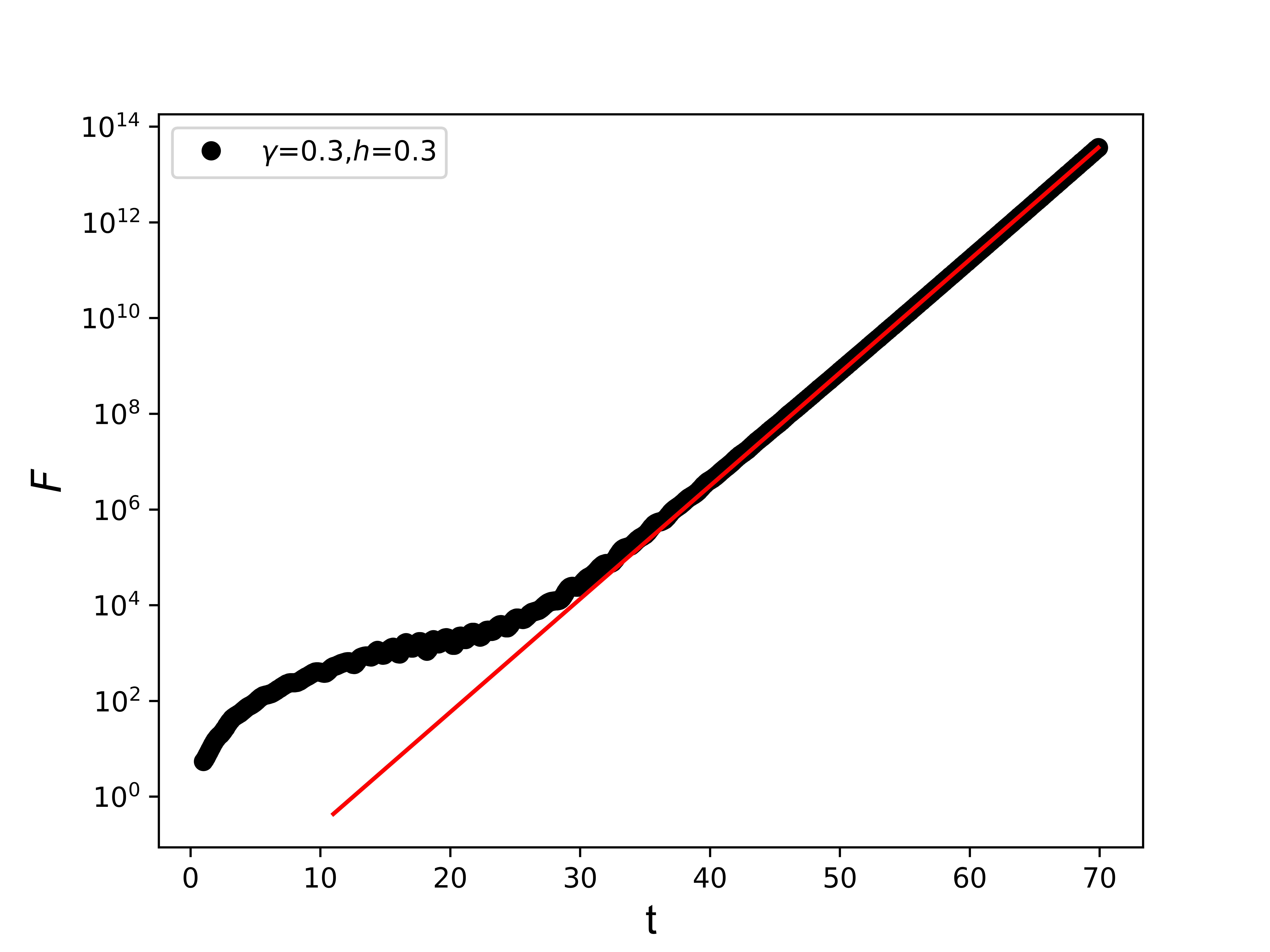
Figure 2: The figure presents the time evolution of the quantum Fisher information (QFI) for a set of parameters of the Hamiltonian, $h=0.3$ and $\gamma=0.3$. We observe that an exponential scaling emerges, which depends on $\gamma$ and kicks in at a time that varies with the parameter values. The red line is an exponential fitting of the long-time behavior of the QFI.

The effects of MIPT on QFI, which can potentially manifest itself in a non-analytic behaviour of QFI accross the MIPT, are partially concealed by this exponential time dependence. In order to unveil the singular part of QFI one can suitably factor out the exponential scaling. This procedure provides a smooth mapping which leaves unaltered the analytic properties of the QFI. Indeed, when examining the long-time behavior of the QFI, one can decompose the QFI in terms of the eigenmodes $k$, each dominated by a specific time-dependent exponential factor

$$F=\sum_{k}F_{k}e^{4\Gamma_{k}t}$$ (20)

where, we recall, $\Gamma_{k}$’s are the imaginary part of the eigenvalues $\epsilon_{k}$, while $F_{k}$’s are time-independent coefficients, which are expressed in detail in Appendix B. The $\Gamma_{k}$ functions are continuous with respect to $\gamma$, hence, any divergences of QFI due to the MIPT are to be found in the $F_{k}$ terms. Moreover, one can explicitly relate any divergent behaviour of the QFI to that of an auxiliary function $\bar{F}=\sum_{k}F_{k}$ thanks to the following chain of inequalities

$$\bar{F}<F<e^{\frac{\Gamma_{\rm{max}}}{4}t}\bar{F},$$ (21)

where $\Gamma_{\rm{max}}$ is the maximum value of the imaginary part of the spectrum, which is a continuous function of $\gamma$. This shows that $\bar{F}$ retains the same divergent behaviour of $F$, but its study is considerably more amenable to numerical analysis, due to the absence of the exponential factors $e^{4\Gamma_{k}t}$. In Fig. 3 we plot the dependence of $\bar{F}$ on $\gamma$, which clearly displays a peak at the critical value $\gamma=\gamma_{c}$, with a distinctive asymmetric behaviour as the criticality is approached from either above or below.

We analytically derive the singular part of the QFI (see Appendix B), which scales as

$$F\sim F_{k_{c}}\propto\left\{\begin{split}&(\gamma-\gamma_{c})^{-3}\hskip 14.22636pt\gamma>\gamma_{c}\\ &(\gamma_{c}-\gamma)^{-2}\hskip 14.22636pt\gamma<\gamma_{c},\end{split}\right.$$ (22)

where $k_{c}=\arccos\left(-h\right)$ is a critical mode, i.e. the mode which is gapless at the MIPT. These features are in accordance with the numerical results shown in Fig. 3 and confirm them as a distinctive signature of the MIPT in the QFI behavior. The non-analytical behaviour of QFI is strictly related to the closing of the gap at criticality. In particular, the different scaling laws as the critical point is approached from above or below $\gamma_{c}$ can be pin-pointed to the different character of the spectrum at the two sides of the criticality. The critical point is in fact an exceptional point [53] of the model. This is associated to a gap of the model which is real for $\gamma<\gamma_{c}$ and imaginary for $\gamma>\gamma_{c}$. Heuristically, these qualitatively different behaviours of the spectrum reflect the distinct characters of the two phases: (i) $\gamma<\gamma_{c}$ in which, as in standard QPT, the dynamics is dominated by coherent phenomena, with a real energy gap, and (ii) $\gamma>\gamma_{c}$ where the dynamics is driven by measurement processes, entailing a dissipative, Zeno-like gap. In both cases, the divergence of the QFI manages to capture the closing of the gap, and discriminates the distinctive features of the two phases through the asymmetry of scaling laws.

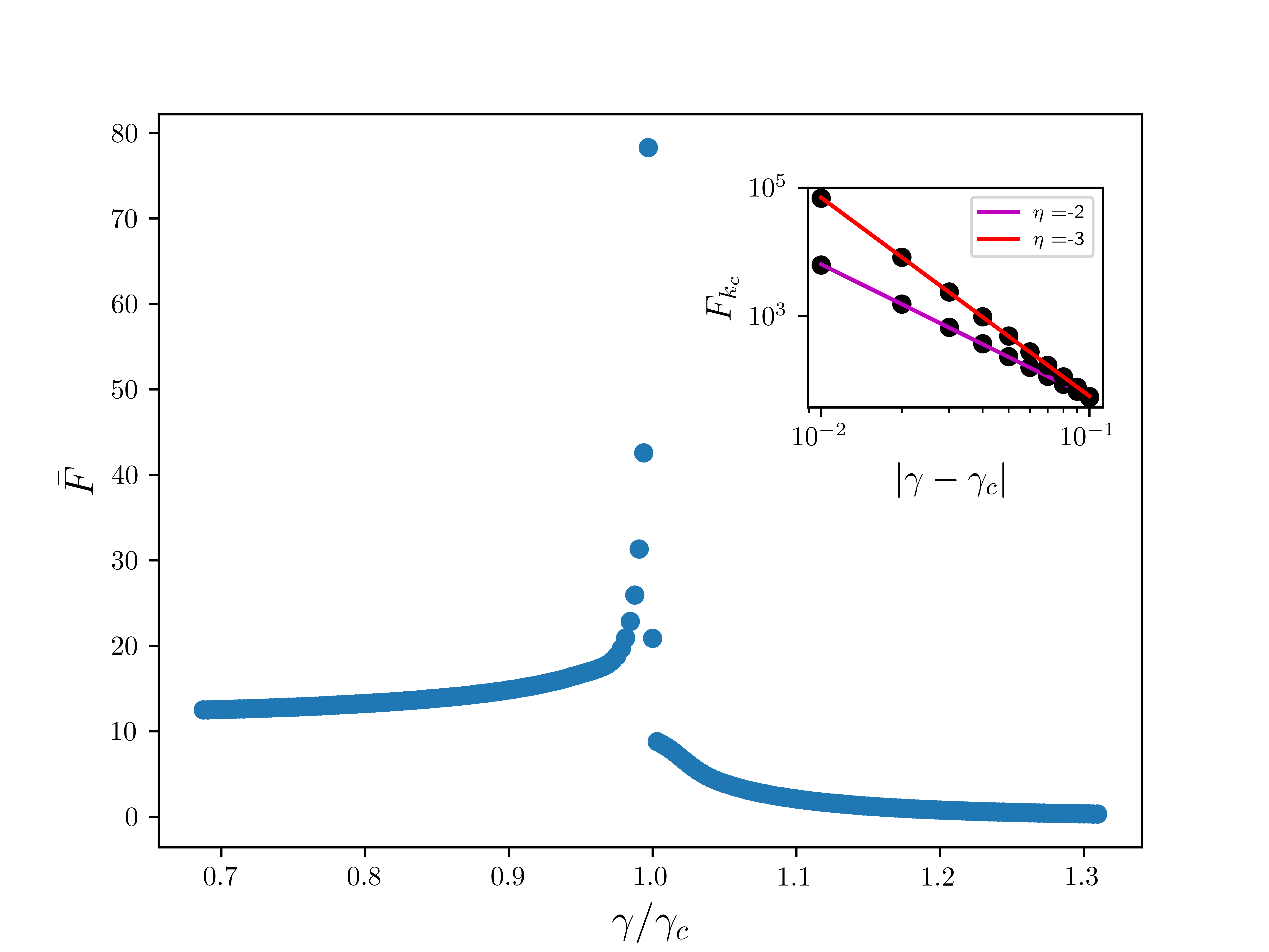
Figure 3: The main figure illustrates the variation of the $\bar{F}$ for different values of $\gamma$, where $\gamma_{c}$ represents the critical value of the measurement rate (h = 0.6). In the inset, presented on a log-log plot, we depict the scaling behavior of the critical mode as reported in Eq. (22) ($F_{k_{c}}\propto 1/|\gamma-\gamma_{c}|^{\eta}$), in magenta the scaling for $\gamma<\gamma_{c}$ and in red for $\gamma>\gamma_{c}$.

5 Conclusion

We have studied the impact of the MIPT on the QFI of a one-dimensional Ising chain subjected to a transverse magnetic field. Our analysis reveals a change in the scaling behaviour of the QFI accross the transition point, with a super-extensive (sub-extensive) scaling law for values of the measuring rate $\gamma$ below (above) its critical value $\gamma_{c}=\sqrt{h-1}$. This is revealed by the presence of multi-partite entanglement for $\gamma<\gamma_{c}$, not signalled for $\gamma>\gamma_{c}$. This behaviour is consistent with the entanglement phase transition observed through the entanglement entropy [4, 5, 6]. The QFI, however, provides a new insight into the multipartite nature of the entaglement associated with the two phases, demostrating its usefulness as a resource for quantum metrology.
Additionally, we have shown that the MIPT can be revealed through the divergent behaviour of the QFI with respect to the measuring rate. This non-trivial finding parallels the analogous non-analyticity of the QFI accross standard QPTs, when the QFI is evaluated with respect to the parameter driving the transition [22]. Our findings provide new insights into the behavior of quantum systems subjected to MIPT, and open up the possibility of extending this approach to a general class of transitions in non-equilibrium physics, with competition between closed, open and measurements induced dynamics.
During the preparation of this manuscript the authors became aware of the related work [57], which analyses multipartite entanglement across MIPT.

Acknowledgments— This work was supported by Italian Ministry of University and Research (MUR). The authors are grateful to Dr. Federico Roccati for useful discussions.

Appendix A Appendix A

To ensure clarity and self-consistency to the work, in this Appendix we provide a set of information and details on the non-Hermitian Hamiltonian in Eq. (3) of the main text. Firstly, we employ the Jordan-Wigner transformation

$$\left\{\begin{split}&\sigma_{i}^{x}=\prod_{j<i}\left(2n_{i}-1\right)\left(c_{i}+c_{i}^{\dagger}\right)\\ &\sigma_{i}^{z}=1-2c_{i}^{\dagger}c_{i}\end{split}\right.$$ (23)

to rewrite our Hamiltonian in fermionic language. Subsequently, we move to the momentum space through the Fourier transform $c_{j}=\frac{e^{i\pi/4}}{\sqrt{N}}\sum_{k}e^{ikj}c_{k}$. This results in the expression of Eq. (4) of the main text

$$H=\sum_{k}\left(\begin{matrix}c^{\dagger}_{k}&c_{-k}\end{matrix}\right)M_{k}\left(\begin{matrix}c_{k}\\ c_{-k}^{\dagger}\end{matrix}\right),$$ (24)

where

$$M_{k}=\left(\begin{matrix}\alpha_{k}&\beta_{k}\\ \beta_{k}&-\alpha_{k}\end{matrix}\right).$$ (25)

In this work, every time we considered the expression of the Hamiltonian in the momentum space, we worked with periodic boundary conditions on the spin chain and an even number of fermions. This corresponded to use anti-periodic boundary conditions for the fermionic chain with

$$k=\left\{\frac{\left(2n-1\right)\pi}{N}\left|n=1,...,\frac{L}{2}\right.\right\},$$ (26)

where only the positive values were used due to the symmetries of the Hamiltonian. We also note that in Eq. (24), a constant term was neglected as it does not affect the system’s dynamics. The spectrum of Eq.(25), denoted as $\epsilon_{k}=\pm\sqrt{\alpha_{k}^{2}+\beta_{k}^{2}}=\pm E_{k}\pm i\Gamma_{k}$, possesses both real and imaginary parts. The real and imaginary parts are denoted as $E_{k}=\Re{(\epsilon_{k})}$ and $\Gamma_{k}=\Im{(\epsilon_{k})}$, respectively. It is important to note that the convention on the sign can be chosen independently for each $k$ in the system’s spectrum. In this study, we have chosen the convention such that $\Gamma_{k}\leq 0$ always. Furthermore, it is worth noting that there exists a critical value of $k$, given by $k_{c}=\arccos\left(-h\right)$, where $\epsilon_{k}$ is real for $\gamma\leq\gamma_{c}$ and imaginary for $\gamma>\gamma_{c}$. This peculiar behavior of non-Hermitian systems is illustrated in Fig.4, where the behavior of the spectrum is reported for various values of $\gamma$.

Figure 4: The figure presents the spectrum of the Hamiltonian in Eq. (24) for different values of the measurement rate $\gamma$. The upper panel displays the real part of the spectrum, gapped at $\pm k_{c}$ for $\gamma/\gamma_{c}<1$, while it becomes gapless for $\gamma/\gamma_{c}\geq 1$. On the other hand, the lower panel shows the behavior of the imaginary part, which attains its maximum value $\Gamma_{k}=0$ at $\pm k_{c}$ for $\gamma\leq\gamma_{c}$, whereas it remains non-zero for $\gamma>\gamma_{c}$.

The time-dependent state can be computed easily due to the initial state’s well-defined parity and translation invariance. As a result, the dynamics can be decomposed into $N/2$ independent ones

$$\left|\psi\right\rangle=\prod_{k}\left|\psi_{k}\right\rangle.$$ (27)

If we denote with $\left|\tilde{\psi}\right\rangle=\left(u^{t}_{k}+v^{t}_{k}c^{\dagger}_{k}c^{\dagger}_{-k}\right)\left|0\right\rangle$ the unnormalized $k$ state we can easily see that its dynamics is given by

$$i\frac{d}{dt}\left(\begin{matrix}u^{t}_{k}\\ v^{t}_{k}\end{matrix}\right)=M_{k}\left(\begin{matrix}u^{t}_{k}\\ v^{t}_{k}\end{matrix}\right),$$ (28)

whose solution is given in Eq. (19) of the main text, with initial condition given by

$$\left(\begin{matrix}u_{k}\\ v_{k}\end{matrix}\right)=\frac{1}{\sqrt{2\epsilon_{k}\left(\epsilon_{k}-z_{k}\right)}}\left(\begin{matrix}\epsilon_{k}-z_{k}\\ y_{k}\end{matrix}\right),$$ (29)

where $z_{k}=2\left(h+\cos\left(k\right)\right)$ and $y_{k}=2\sin\left(k\right)$.

Appendix B Appendix B

This Appendix presents the derivation of the QFI expression for the non-Hermitian quantum quench. As mentioned in the main text, the state at time $t$ can be expressed as a function of the initial state $\left|\psi_{0}\right\rangle$, using the general form

$$\left|\psi\left(t\right)\right\rangle=N\left(t\right)e^{-iH_{\mathrm{eff}}t}\left|\psi_{0}\right\rangle.$$ (30)

To obtain the QFI, it is necessary to compute the derivative of the state with respect to a parameter of interest, which can be expressed as

$$\left|\partial_{\lambda}\psi\right\rangle=\left(\partial_{\lambda}N\left(t\right)e^{-iH_{\mathrm{eff}}t}+N\left(t\right)\partial_{\lambda}e^{-iH_{\mathrm{eff}}t}\right)\left|\psi_{0}\right\rangle.$$ (31)

It is important to note that the derivative of the exponential term in the last term of Eq. (31) should be carefully considered, as $\partial_{\lambda}H$ and $H$ do not commute. The Sneddon’s formula [58] allows us to express Eq. (31) as

$$\begin{split}\left|\partial_{\lambda}\psi\right\rangle&=\left(\tfrac{\partial_{\lambda}N\left(t\right)}{N\left(t\right)}+\int_{0}^{t}ds\exp{\left(-iH_{\mathrm{eff}}s\right)}\partial_{\lambda}\left(-iH_{\mathrm{eff}}\right)\exp{\left(iH_{\mathrm{eff}}s\right)}\right)\left|\psi\right\rangle\\ &=\left(\tfrac{\partial_{\lambda}N\left(t\right)}{N\left(t\right)}+O_{\lambda}\right)\left|\psi\right\rangle,\end{split}$$ (32)

and applying the general definition of the QFI for pure states, we can easily obtain

$$\frac{F}{4} =\left\langle\partial_{\lambda}\psi\right|\left.\partial_{\lambda}\psi\right\rangle-\left|\left\langle\partial_{\lambda}\psi\right|\left.\psi\right\rangle\right|^{2}$$ (33)

$$=\left\langle\psi\right|\left[\left(\tfrac{\partial_{\lambda}N}{N}\right)^{*}+O_{\lambda}^{\dagger}\right]\left[\tfrac{\partial_{\lambda}N}{N}+O_{\lambda}\right]\left|\psi\right\rangle-\left[\tfrac{\partial_{\lambda}N}{N}+\left\langle\psi\right|O_{\lambda}\left|\psi\right\rangle\right]\left[\left(\tfrac{\partial_{\lambda}N}{N}\right)^{*}+\left\langle\psi\right|O_{\lambda}^{\dagger}\left|\psi\right\rangle\right]$$

$$=\left\langle\psi\right|O_{\lambda}^{\dagger}O_{\lambda}\left|\psi\right\rangle-\left\langle\psi\right|O_{\lambda}\left|\psi\right\rangle\left\langle\psi\right|O_{\lambda}^{\dagger}\left|\psi\right\rangle.$$

The closed expression for the operator $O_{\gamma}$ reported in the main text can be obtained by explicitly computing the derivative of the Hamiltonian with respect to $\gamma$, which yields the following result

$$O_{\gamma}=-\int_{0}^{t}ds\hskip 2.84544pte^{-iH_{\mathrm{eff}}s}\sum_{k}\left(\begin{matrix}c^{\dagger}_{k}&c_{-k}\end{matrix}\right)\left(\begin{matrix}1&0\\ 0&-1\end{matrix}\right)\left(\begin{matrix}c_{k}c^{\dagger}_{-k}\end{matrix}\right)e^{iH_{\mathrm{eff}}s}-\tfrac{Nt}{4}.$$ (34)

After evaluating the equation of motion for the operator $c_{k}$, we can rewrite Eq. (34) as

$$O_{\gamma}=\sum_{k}\left(\begin{matrix}c^{\dagger}_{k}&c_{-k}\end{matrix}\right)\left[\int_{0}^{t}ds\hskip 2.84544pte^{-iM_{k}s}\left(\begin{matrix}1&0\\ 0&-1\end{matrix}\right)e^{iM_{k}s}\right]\left(\begin{matrix}c_{k}\\ c^{\dagger}_{-k}\end{matrix}\right)-\tfrac{Nt}{4}.$$ (35)

At this point, following a series of tedious but straightforward algebraic manipulations, we arrive at the conclusion that

$$O_{\gamma}=-\sum_{k}\left(\begin{matrix}c^{\dagger}_{k}&c_{-k}\end{matrix}\right)R_{k}\left(\begin{matrix}c_{k}\\ c^{\dagger}_{-k}\end{matrix}\right)-\tfrac{Nt}{4},$$ (36)

where

$$\begin{split}R_{k}&=\left(\begin{matrix}A_{k}&B_{k}\\ C_{k}&-A_{k}\end{matrix}\right)=\\ &=\left(\begin{matrix}\frac{t\alpha_{k}^{2}}{\epsilon_{k}^{2}}+\frac{\sin\left(2\epsilon_{k}t\right)}{2\epsilon_{k}^{3}}\beta_{k}^{2}&\frac{\alpha_{k}\beta_{k}t}{\epsilon_{k}^{2}}+\frac{2\beta_{k}\sin^{2}\left(\epsilon_{k}t\right)\epsilon_{k}i-\alpha_{k}\beta_{k}\sin\left(2\epsilon_{k}t\right)}{2\epsilon_{k}^{3}}\\ \frac{\alpha_{k}\beta_{k}t}{\epsilon_{k}^{2}}-\frac{2\beta_{k}\sin^{2}\left(\epsilon_{k}t\right)\epsilon_{k}i+\alpha_{k}\beta_{k}\sin\left(2\epsilon_{k}t\right)}{2\epsilon_{k}^{3}}&-\frac{t\alpha_{k}^{2}}{\epsilon_{k}^{2}}-\frac{\sin\left(2\epsilon_{k}t\right)}{2\epsilon_{k}^{3}}\beta_{k}^{2}\end{matrix}\right)\\ \end{split}$$ (37)

Using the expression of Eq. (17) of the main text, we can evaluate the expectation value of Eq.(33), resulting in the following expression

$$\begin{split}\frac{F}{4}&=\left\langle\psi\right|O_{\lambda}^{\dagger}O_{\lambda}\left|\psi\right\rangle-\left\langle\psi\right|O_{\lambda}\left|\psi\right\rangle\left\langle\psi\right|O_{\lambda}^{\dagger}\left|\psi\right\rangle=\\ &=\sum_{k}\left[\frac{\left[|u^{t}_{k}|^{2}\left(|A_{k}|^{2}+|C_{k}|^{2}\right)-2\Re\left(u^{t*}_{k}v^{t}_{k}\left(-A_{k}B^{*}_{k}+C_{k}A^{*}_{k}\right)\right)+|v^{t}_{k}|^{2}\left(|A_{k}|^{2}+|B_{k}|^{2}\right)\right]}{|u^{t}_{k}|^{2}+|v^{t}_{k}|^{2}}+\right.\\ &-\left.\left|\frac{\left(-|u_{k}^{t}|^{2}A_{k}-C_{k}u_{k}^{t*}v^{t}_{k}-B_{k}u^{t}_{k}v_{k}^{t*}+A_{k}|v^{t}_{k}|^{2}\right)}{|u^{t}_{k}|^{2}+|v^{t}_{k}|^{2}}\right|^{2}\right].\end{split}$$ (38)

When examining the long-time behavior of the QFI, it becomes evident that we can factorize the exponential scaling. This can be seen from

$$\left\{\begin{split}&A_{k}=\frac{i\beta^{2}_{k}}{4\epsilon_{k}^{3}}e^{2i\epsilon_{k}t}=\tilde{A}_{k}e^{2i\epsilon_{k}t},\\ &B_{k}=i\frac{-\beta_{k}\epsilon_{k}-\alpha_{k}\beta_{k}}{4\epsilon_{k}^{3}}e^{2i\epsilon_{k}t}=\tilde{B}_{k}e^{2i\epsilon_{k}t},\\ &C_{k}=i\frac{\beta_{k}\epsilon_{k}+\alpha_{k}\beta_{k}}{4\epsilon_{k}^{3}}e^{2i\epsilon_{k}t}=\tilde{B}_{k}e^{2i\epsilon_{k}t}.\end{split}\right.$$ (39)

These scaling laws are valid for all values of $k$ and $\gamma$, except for $k_{c}$ when $\gamma<\gamma_{c}$. To compute the long time behavior of the QFI, we can evaluate the expectation value by using the ground state of the effective Hamiltonian [53]. We denote with $\tilde{u}_{k},\tilde{v}_{k}$ its coefficients. Then it follows that the long time behavior of the quantum Fisher information is

$$\begin{split}&F=\sum_{k}\left[\frac{\left(|\tilde{u}_{k}|^{2}\left(|\tilde{A}_{k}|^{2}+|\tilde{C}_{k}|^{2}\right)-2\Re\left(\tilde{u}_{k}\tilde{v}_{k}^{*}\left(\tilde{A}^{*}_{k}\tilde{C}_{k}-\tilde{A}_{k}\tilde{B}^{*}_{k}\right)\right)+|\tilde{v}_{k}|^{2}\left(|\tilde{A}_{k}|^{2}+|\tilde{B}_{k}|^{2}\right)\right)e^{4\Gamma_{k}t}}{\left(|\tilde{u}_{k}|^{2}+|\tilde{v}_{k}|^{2}\right)}\right.+\\ &-\left.\frac{\left|\left(-\tilde{A}_{k}|\tilde{u}_{k}|^{2}-\tilde{C}_{k}\tilde{u}_{k}^{*}\tilde{v}_{k}-\tilde{B}_{k}\tilde{u}_{k}\tilde{v}^{*}_{k}+\tilde{A}_{k}|\tilde{v}|^{2}\right)\right|^{2}e^{4\Gamma_{k}t}}{\left(\left(|\tilde{u}_{k}|^{2}+|\tilde{v}_{k}|^{2}\right)\right)^{2}}\right]=\\ &=\sum_{k}F_{k}e^{4\Gamma_{k}t}.\end{split}$$ (40)

The critical mode’s expression of the QFI can be determined analytically by evaluating Eq.(40) for $k_{c}=\arccos(-h)$. When $\gamma>\gamma_{c}$, the QFI can be computed using the expressions provided in Eq.(39). In contrast, when $\gamma<\gamma_{c}$, the linear term in $t$ becomes the leading term in the long time approximation of Eq. (37). This phenomenon is responsible for the difference in the scaling laws of Eq. (22) of the main text.

References

- [1] Davide Rossini and Ettore Vicari. “Measurement-induced dynamics of many-body systems at quantum criticality”. Phys. Rev. B 102, 035119 (2020).
- [2] Xiangyu Cao, Antoine Tilloy, and Andrea De Luca. “Entanglement in a fermion chain under continuous monitoring”. SciPost Phys. 7, 024 (2019).
- [3] O. Alberton, M. Buchhold, and S. Diehl. “Entanglement transition in a monitored free-fermion chain: From extended criticality to area law”. Phys. Rev. Lett. 126, 170602 (2021).
- [4] Alberto Biella and Marco Schiró. “Many-body quantum Zeno effect and measurement-induced subradiance transition”. Quantum 5, 528 (2021).
- [5] Xhek Turkeshi, Alberto Biella, Rosario Fazio, Marcello Dalmonte, and Marco Schiró. “Measurement-induced entanglement transitions in the quantum Ising chain: From infinite to zero clicks”. Phys. Rev. B 103, 224210 (2021).
- [6] Xhek Turkeshi and Marco Schiró. “Entanglement and correlation spreading in non-Hermitian spin chains”. Phys. Rev. B 107, L020403 (2023).
- [7] Takaaki Minato, Koudai Sugimoto, Tomotaka Kuwahara, and Keiji Saito. “Fate of measurement-induced phase transition in long-range interactions”. Phys. Rev. Lett. 128, 010603 (2022).
- [8] Michael J. Gullans and David A. Huse. “Dynamical purification phase transition induced by quantum measurements”. Phys. Rev. X 10, 041020 (2020).
- [9] Michael J. Gullans and David A. Huse. “Scalable probes of measurement-induced criticality”. Phys. Rev. Lett. 125, 070606 (2020).
- [10] Amos Chan, Rahul M. Nandkishore, Michael Pretko, and Graeme Smith. “Unitary-projective entanglement dynamics”. Phys. Rev. B 99, 224307 (2019).
- [11] Brian Skinner, Jonathan Ruhman, and Adam Nahum. “Measurement-induced phase transitions in the dynamics of entanglement”. Phys. Rev. X 9, 031009 (2019).
- [12] Adam Nahum, Sthitadhi Roy, Brian Skinner, and Jonathan Ruhman. “Measurement and entanglement phase transitions in all-to-all quantum circuits, on quantum trees, and in Landau-Ginsburg theory”. PRX Quantum 2, 010352 (2021).
- [13] Soonwon Choi, Yimu Bao, Xiao-Liang Qi, and Ehud Altman. “Quantum error correction in scrambling dynamics and measurement-induced phase transition”. Phys. Rev. Lett. 125, 030505 (2020).
- [14] Shengqi Sang, Yaodong Li, Tianci Zhou, Xiao Chen, Timothy H. Hsieh, and Matthew P.A. Fisher. “Entanglement negativity at measurement-induced criticality”. PRX Quantum 2, 030313 (2021).
- [15] Ali Lavasani, Yahya Alavirad, and Maissam Barkeshli. “Measurement-induced topological entanglement transitions in symmetric random quantum circuits”. Nature Physics 17, 342–347 (2021). arXiv:2004.07243.
- [16] G. Mussardo, Ship Navigation, and Northern Sea Route. “Statistical field theory : an introduction to exactly solved models in statistical physics”. Page 755. Oxford University Press. (2010).
- [17] Paolo Zanardi, Matteo G A Paris, and Lorenzo Campos Venuti. “Quantum criticality as a resource for quantum estimation”. Phys. Rev. A 78, 042105 (2008).
- [18] Carmen Invernizzi, Michael Korbman, Lorenzo Campos Venuti, and Matteo G. A. Paris. “Optimal quantum estimation in spin systems at criticality”. Phys. Rev. A 78, 042106 (2008).
- [19] Mankei Tsang. “Quantum transition-edge detectors”. Phys. Rev. A 88, 021801 (2013).
- [20] P. A. Ivanov and D. Porras. “Adiabatic quantum metrology with strongly correlated quantum optical systems”. Phys. Rev. A 88, 023803 (2013).
- [21] M Bina, I Amelio, and M. G. A. Paris. “Dicke coupling by feasible local measurements at the superradiant quantum phase transition”. Phys. Rev. E 93, 052118 (2016).
- [22] Irénée Frérot and Tommaso Roscilde. “Quantum critical metrology”. Phys. Rev. Lett. 121, 020402 (2018).
- [23] Toni L. Heugel, Matteo Biondi, Oded Zilberberg, and R. Chitra. “Quantum transducer using a parametric driven-dissipative phase transition”. Phys. Rev. Lett. 123, 173601 (2019).
- [24] Louis Garbe, Matteo Bina, Arne Keller, Matteo G. A. Paris, and Simone Felicetti. “Critical quantum metrology with a finite-component quantum phase transition”. Phys. Rev. Lett. 124, 120504 (2020).
- [25] Peter A Ivanov. “Steady-state force sensing with single trapped ion”. Phys. Scr. 95, 025103 (2020).
- [26] Victor Montenegro, Utkarsh Mishra, and Abolfazl Bayat. “Global sensing and its impact for quantum many-body probes with criticality”. Phys. Rev. Lett. 126, 200501 (2021).
- [27] Francesco Albarelli and Rafał Demkowicz-Dobrzański. “Probe incompatibility in multiparameter noisy quantum metrology”. Phys. Rev. X 12, 011039 (2022).
- [28] R. Di Candia, F. Minganti, K. V. Petrovnin, G. S. Paraoanu, and S. Felicetti. “Critical parametric quantum sensing” (2021).
- [29] Giovanni Di Fresco, Bernardo Spagnolo, Davide Valenti, and Angelo Carollo. “Multiparameter quantum critical metrology”. SciPost Phys. 13, 077 (2022).
- [30] Angelo Carollo, Davide Valenti, and Bernardo Spagnolo. “Geometry of quantum phase transitions”. Phys. Rep. 838, 1–72 (2020).
- [31] Philipp Hyllus, Wiesław Laskowski, Roland Krischek, Christian Schwemmer, Witlef Wieczorek, Harald Weinfurter, Luca Pezzé, and Augusto Smerzi. “Fisher information and multiparticle entanglement”. Phys. Rev. A 85, 022321 (2012).
- [32] Géza Tóth. “Multipartite entanglement and high-precision metrology”. Phys. Rev. A 85, 022322 (2012).
- [33] Helmut Strobel, Wolfgang Muessel, Daniel Linnemann, Tilman Zibold, David B. Hume, Luca Pezzè, Augusto Smerzi, and Markus K. Oberthaler. “Fisher information and entanglement of non-Gaussian spin states”. Science 345, 424–427 (2014).
- [34] Philipp Hauke, Markus Heyl, Luca Tagliacozzo, and Peter Zoller. “Measuring multipartite entanglement through dynamic susceptibilities”. Nature Physics 12, 778–782 (2016).
- [35] Carl W. Helstrom. “Quantum detection and estimation theory”. Academic Press. (1976).
- [36] Magdalena Szczykulska, Tillmann Baumgratz, and Animesh Datta. “Multi-parameter quantum metrology”. Adv. Phys. X 1, 621–639 (2016).
- [37] Francesco Albarelli, Marco Barbieri, M.G. Genoni, and Ilaria Gianani. “A perspective on multiparameter quantum metrology: From theoretical tools to applications in quantum imaging”. Phys. Lett. A 384, 126311 (2020).
- [38] Manuel A. Ballester. “Entanglement is not very useful for estimating multiple phases”. Phys. Rev. A 70, 032310 (2004).
- [39] Cyril Vaneph, Tommaso Tufarelli, and Marco G. Genoni. “Quantum estimation of a two-phase spin rotation”. Quantum Meas. Quantum Metrol. 1, 12–20 (2013).
- [40] M. G. Genoni, M. G. A. Paris, G. Adesso, H. Nha, P. L. Knight, and M. S. Kim. “Optimal estimation of joint parameters in phase space”. Phys. Rev. A 87, 012107 (2013).
- [41] Haidong Yuan and Chi-Hang Fred Fung. “Optimal feedback scheme and universal time scaling for Hamiltonian parameter estimation”. Phys. Rev. Lett. 115, 110401 (2015).
- [42] Dominic W. Berry, Mankei Tsang, Michael J. W. Hall, and Howard M. Wiseman. “Quantum Bell-Ziv-Zakai bounds and Heisenberg limits for waveform estimation”. Phys. Rev. X 5, 031018 (2015).
- [43] Manuel Gessner, Luca Pezzè, and Augusto Smerzi. “Sensitivity bounds for multiparameter quantum metrology”. Phys. Rev. Lett. 121, 130503 (2018).
- [44] Jesús Rubio and Jacob Dunningham. “Bayesian multiparameter quantum metrology with limited data”. Phys. Rev. A 101, 032114 (2020).
- [45] Angelo Carollo, Bernardo Spagnolo, Alexander A. Dubkov, and Davide Valenti. “On quantumness in multi-parameter quantum estimation”. J. Stat. Mech. Theory Exp. 2019, 094010 (2019).
- [46] Francesco Albarelli, Jamie F. Friel, and Animesh Datta. “Evaluating the Holevo Cramér-Rao bound for multiparameter quantum metrology”. Phys. Rev. Lett. 123, 200503 (2019).
- [47] Jasminder S. Sidhu, Yingkai Ouyang, Earl T. Campbell, and Pieter Kok. “Tight bounds on the simultaneous estimation of incompatible parameters”. Phys. Rev. X 11, 011028 (2021).
- [48] Mankei Tsang, Francesco Albarelli, and Animesh Datta. “Quantum semiparametric estimation”. Phys. Rev. X 10, 031023 (2020).
- [49] Rafał Demkowicz-Dobrzański, Wojciech Górecki, and Mădălin Guţă. “Multi-parameter estimation beyond quantum Fisher information”. J. Phys. A Math. Theor. 53, 363001 (2020).
- [50] Elliott H. Lieb, Theodore Schultz, and Daniel Mattis. “Two soluble models of an antiferromagnetic chain”. Ann. Phys. (N. Y). 16, 407–466 (1961).
- [51] E Barouch and B M McCoy. “Statistical mechanics of the XY model. II. Spin-correlation functions”. Phys. Rev. A 3, 786–804 (1971).
- [52] Glen Bigan Mbeng, Angelo Russomanno, and Giuseppe E. Santoro. “The quantum Ising chain for beginners” (2020).
- [53] Tony E. Lee and Ching-Kit Chan. “Heralded magnetism in non-Hermitian atomic systems”. Phys. Rev. X 4, 041001 (2014).
- [54] Sammy Ragy, Marcin Jarzyna, and Rafał Demkowicz-Dobrzański. “Compatibility in multiparameter quantum metrology”. Phys. Rev. A 94, 052108 (2016).
- [55] Jing Liu, Haidong Yuan, Xiao-Ming Lu, and Xiaoguang Wang. “Quantum Fisher information matrix and multiparameter estimation”. Journal of Physics A: Mathematical and Theoretical 53, 023001 (2019).
- [56] Michael Skotiniotis, Pavel Sekatski, and Wolfgang Dür. “Quantum metrology for the Ising Hamiltonian with transverse magnetic field”. New Journal of Physics 17, 073032 (2015).
- [57] Alessio Paviglianiti and Alessandro Silva. “Multipartite entanglement in the measurement-induced phase transition of the quantum ising chain” (2023). arXiv:2302.06477.
- [58] Ravinder Rupchand Puri. “Algebra of the exponential operator”. Pages 37–53. Springer Berlin Heidelberg. Berlin, Heidelberg (2001).