Over-Parameterization Exponentially Slows Down Gradient Descent for Learning a Single Neuron

Abstract

We revisit the problem of learning a single neuron with ReLU activation under Gaussian input with square loss. We particularly focus on the over-parameterization setting where the student network has $n\geq 2$ neurons. We prove the global convergence of randomly initialized gradient descent with a $O\left(T^{-3}\right)$ rate. This is the first global convergence result for this problem beyond the exact-parameterization setting ($n=1$) in which the gradient descent enjoys an $\exp(-\Omega(T))$ rate. Perhaps surprisingly, we further present an $\Omega\left(T^{-3}\right)$ lower bound for randomly initialized gradient flow in the over-parameterization setting. These two bounds jointly give an exact characterization of the convergence rate and imply, for the first time, that over-parameterization can exponentially slow down the convergence rate. To prove the global convergence, we need to tackle the interactions among student neurons in the gradient descent dynamics, which are not present in the exact-parameterization case. We use a three-phase structure to analyze GD’s dynamics. Along the way, we prove gradient descent automatically balances student neurons, and use this property to deal with the non-smoothness of the objective function. To prove the convergence rate lower bound, we construct a novel potential function that characterizes the pairwise distances between the student neurons (which cannot be done in the exact-parameterization case). We show this potential function converges slowly, which implies the slow convergence rate of the loss function.

1 Introduction

In recent years, theoretical explanations of the success of gradient descent (GD) on training deep neural networks emerge as an important problem. A prominent line of work Allen-Zhu et al. [2018], Du et al. [2018c], Jacot et al. [2018], Safran and Shamir [2018], Chizat et al. [2019] suggests that over-parameterization plays a key role in the successful training of neural networks.

However, the drawback of over-parameterization is under-explored. In this paper, we consider training two-layer ReLU networks, with a particular focus on learning a single neuron in the over-parameterization setting. We give a rigorous proof for the following surprising phenomenon:

Over-parameterization exponentially slows down the convergence of gradient descent.

Specifically, we consider two-layer ReLU networks with $n$ neurons and input dimension $d$:

$$\bm{x}\to\sum_{i=1}^{n}[\bm{w}_{i}^{\top}\bm{x}]_{+},$$ (1)

where $[x]_{+}=\max\{0,x\}$ denotes the ReLU function, $\bm{w}_{1},\ldots,\bm{w}_{n}\in\mathbf{R}^{d}$ are $n$ neurons. The input $\bm{x}\sim\mathcal{N}(0,I)$ follows a standard Gaussian distribution.

We consider the teacher-student setting, where a student network is trained to learn a ground truth teacher network. Following the architecture (1), the student network $f:\mathbf{R}^{d}\to\mathbf{R}$ is given by $f(\bm{x})=\sum_{i=1}^{n}[\bm{w}_{i}^{\top}\bm{x}]_{+},$ where $\bm{w}_{1},\ldots,\bm{w}_{n}\in\mathbf{R}^{d}$ are $n$ student neurons. Similarly, the teacher network is given by $f^{*}(\bm{x})=\sum_{i=1}^{m}[\bm{v}_{i}^{\top}\bm{x}]_{+}$, where $\bm{v}_{1},\ldots,\bm{v}_{m}\in\mathbf{R}^{d}$ are $m$ teacher neurons. It is natural to study the square loss:

$$L(\bm{w})=\mathbb{E}_{\bm{x}\sim\mathcal{N}(\bm{0},I)}\left[\frac{1}{2}\left(\sum_{i=1}^{n}[\bm{w}_{i}^{\top}\bm{x}]_{+}-\sum_{i=1}^{m}[\bm{v}_{i}^{\top}\bm{x}]_{+}\right)^{2}\right],$$ (2)

where $\bm{w}=(\bm{w}_{1}^{\top},\bm{w}_{2}^{\top},\ldots,\bm{w}_{n}^{\top})^{\top}\in\mathbf{R}^{n\times d}$ denotes the parameter vector formed by student neurons.

In this paper, we focus on the special case where the teacher network consists of one single neuron $\bm{v}_{1}$, i.e., $m=1$. For simplicity, we omit the subscript and denote $\bm{v}_{1}$ with $\bm{v}$. The student network is initialized with a Gaussian distribution: $\forall 1\leq i\leq n,\bm{w}_{i}(0)\sim\mathcal{N}(\bm{0},\sigma^{2}I)$, ($\sigma\in\mathbf{R}^{+}$ denotes the initialization scale), then trained by gradient descent with a step size $\eta$.

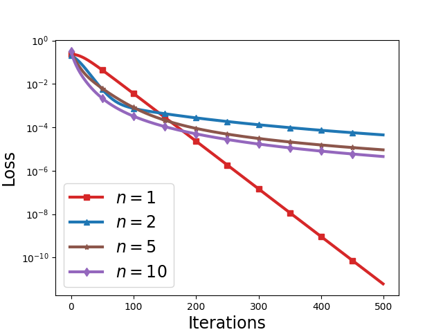
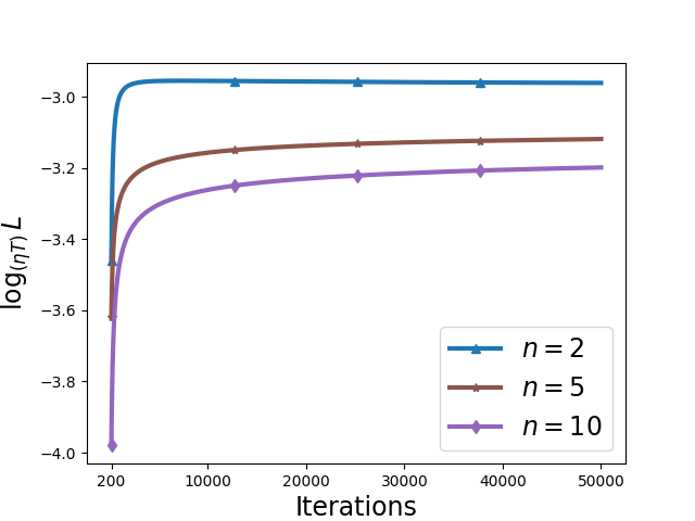
Figure 1: Setting: $\sigma=0.1,\eta=0.05,\|\bm{v}\|=1$. Left: The loss converges much slower when $n>1$, compared to the case of $n=1$. Right: $\log_{(\eta T)}L(\bm{w}(T))$ converges to $-3$, with a small perturbation that converges extremely slow (note if we want $\log_{(\eta T)}\frac{C}{(\eta T)^{3}}\in(-3-\epsilon,-3+\epsilon)$, then $T\geq\frac{1}{\eta}C^{1/\epsilon}$ is needed.)

In this widely-studied setting, we discover a new phenomenon: compared to the exact-parameterized case ($n=1$), the loss $L(\bm{w}(t))$ converges much slower in the over-parameterized case. Empirically (see Figure 1), the slow-down effect happens universally for all $n\geq 2$. Moreover, $\log_{(\eta T)}L(\bm{w}(T))$ has a tendency of converging towards $-3$, which seems to suggest that the convergence rate should be $L(\bm{w}(T))=\Theta(T^{-3})$.

For the exact-parameterized case ($n=1$), Yehudai and Ohad [2020] proved that $L(\bm{w}(t))$ convergences with a linear rate: $L(\bm{w}(t))\leq\exp\left(-\Omega(t)\right)$, which is also validated in Figure 1. For the over-parameterized case, an exact characterization of the convergence rate is given in this paper as $L(\bm{w}(t))=\Theta(t^{-3})$. As a result, we show that (even very mild) over-parameterization exponentially slows down the convergence rate. Specifically, our main results are the following two theorems.

Theorem 1 (Global Convergence, Informal).

For $\forall\delta>0$, suppose the dimension $d=\Omega(\log(n/\delta))$, the initialization scale $\sigma\sqrt{d}=poly(n^{-1})\|\bm{v}\|,$ the learning rate $\eta=poly(\sigma\sqrt{d},n^{-1},\|\bm{v}\|^{-1})$. Then with probability at least $1-\delta$, gradient descent converges to a global minimum with rate $L(\bm{w}(t))\leq poly(n,\|\bm{v}\|,\eta^{-1})t^{-3}$.

Theorem 2 (Convergence Rate Lower Bound, Informal).

Suppose the student network is over-parameterized, i.e., $n\geq 2$. Consider gradient flow: $\frac{\partial\bm{w}(t)}{\partial t}=-\frac{\partial L(\bm{w}(t))}{\partial\bm{w}}.$ If the requirements on $d$ and $\sigma$ in Theorem 1 hold, then with high probability, there exist constants $\Gamma_{1},\Gamma_{2}$ which do not depend on time $t$, such that $\forall t\geq 0,L(\bm{w}(t))\geq{(\Gamma_{1}t+\Gamma_{2})^{-3}}$.

Theorem 1 shows the global convergence of GD, while Theorem 2 provides a convergence rate lower bound. These two bounds together imply an exact characterization of the convergence rate for GD. We further highlight the significance of our contributions below:

$\bullet$ To our knowledge, Theorem 1 is the first global convergence result of gradient descent for the square loss beyond the special exact-parameterization cases of $m=n=1$ [Tian, 2017, Brutzkus and Globerson, 2017, Yehudai and Ohad, 2020, Du et al., 2017] and $m=n=2$ [Wu et al., 2018].

$\bullet$ While over-parameterization is well-known for its benefit in establishing global convergence in the finite-data regime, this is the first work proving it can slow down gradient-based methods.

1.1 Related Works

The problem of learning a single neuron is actually well-understood and can be solved with minimal assumptions by classical single index models algorithms [Kakade et al., 2011]. For learning a single-neuron, Brutzkus and Globerson [2017], Tian [2017], Soltanolkotabi [2017] proved convergence for GD assuming Gaussian input distribution, which was later improved by Yehudai and Ohad [2020] who proved linear convergence of GD for learning one single neuron properly. These results are also generalized to learning a convolutional filter [Goel et al., 2018, Du et al., 2017, 2018a, Zhou et al., 2019, Liu et al., 2019]. These works only focus on the exact-parameterization setting, while we focus on the over-parameterization setting.

Another direction focuses on the optimization landscape. Safran and Shamir [2018] showed spurious local minima exists for large $m$ in the exact-parameterization setting. Safran et al. [2020] studied problem (2) with orthogonal teacher neurons. They showed that neither one-point strong convexity nor Polyak-Łojasiewicz (PL) condition hold locally near the global minimum. Wu et al. [2018] showed that problem (2) has no spurious local minima for $m=n=2$. Zhong et al. [2017], Zhang et al. [2019] studied the exact-parameterization setting and showed the local strong convexity of loss and therefore with tensor initialization, GD can converge to a global minimum. Arjevani and Field [2022] proved that over-parameterization annihilates certain types of spurious local minima.

A popular line of works, known as neural tangent kernel (NTK) [Jacot et al., 2018, Chizat et al., 2019, Du et al., 2018c, 2019, Cao and Gu, 2019, Allen-Zhu et al., 2019, Arora et al., 2019, Oymak and Soltanolkotabi, 2020, Zou et al., 2020, Li and Liang, 2018] connects the training of ultra-wide neural networks with kernel methods. Another line of works uses the mean-field analysis to study the training of infinite-width neural networks [Nitanda and Suzuki, 2017, Chizat and Bach, 2018, Wei et al., 2019, Nguyen and Pham, 2020, Fang et al., 2021, Lu et al., 2020]. All of these works considered the finite-data regime and require the neural network to be ultra-wide, sometimes infinitely wide. Their techniques cannot explain the learnability of a single neuron, as pointed out by Yehudai and Shamir [2019].

More related to our works are results on the dynamics of gradient descent in the teacher-student setting. Li and Yuan [2017] studied the exact-parameterized setting and proved convergence for SGD with initialization in a region near identity. Li et al. [2020] showed that GD can learn two-layer networks better than any kernel methods, but their final upper bound of loss is constantly large and no convergence is proven. Zhou et al. [2021] proved local convergence for mildly over-parameterized two-layer networks. While our global convergence analysis uses their idea of establishing a gradient lower bound, we also propose new techniques to get rid of their architectural modifications, and improved their gradient lower bound to yield a tight convergence rate upper bound (see Section 2 for details). Also, Zhou et al. [2021] only provided a local convergence theory, while we prove convergence globally. On the other hand, their results hold for general $m\geq 1$ whereas we only study $m=1$.

The first phase of our analysis is similar to the initial alignment phenomenon in Boursier et al. [2022]. Their analysis also relies on the finite-data regime and the orthogonality of inputs, hence does not apply to our setting.

Similar slow-down effects of over-parameterization on the convergence rate have been observed in other scenarios. Richert et al. [2022] considered error function activation and empirically observed an $O(T^{-2})$ convergence rate. Going beyond neural network training, Dwivedi et al. [2018], Wu and Zhou [2019] showed such a phenomenon for Expectation-Maximization (EM) algorithm on Gaussian mixture models. Zhang et al. [2022] exhibited similar empirical behaviors of GD on Burer–Monteiro factorization, but no rigorous proof was given.

Paper Organization. In Section 2 we describe the main technical challenges in our analysis, and our ideas for addressing them. In section 3 we define some notations and preliminary notions. In Section 4 we formalize the global convergence result (Theorem 1) and provide a proof sketch. In Section 5 we formalize the convergence rate lower bound (Theorem 2) and provide a proof sketch.

2 Technical Overview

Three-Phase Convergence Analysis. Our global convergence analysis is divided into three phases. We define $\theta_{i}$ as the angle between $\bm{w}_{i}$ and $\bm{v}$, and $H\coloneqq\|\bm{v}\|-\sum_{i}\langle\bm{w}_{i},\overline{\bm{v}}\rangle$. Intuitively, $\theta_{i}$ represents the radial difference between teacher and students, while $H$ represents the tangential difference between teacher and students.

When the initialization $\sigma\sqrt{d}$ is small enough, in phase $1$, for every $i\in[n]$, $\theta_{i}$ decreases to a small value while $\|\bm{w}_{i}\|$ remains small. In phase $2$, $\forall i\in[n],\theta_{i}$ remains bounded by a small value while $H$ decreases with an exponential rate. Both $\theta_{i}$ and $H$ being small at the end of phase $2$ implies that GD enters a local region near a global minimum. In phase $3$, we establish the local convergence by proving two properties: a lower bound of gradient, and a regularity condition of student neurons.

Non-Benign Optimization Landscape. Compared to the exact-parameterization setting, the optimization landscape becomes significantly different and much harder to analyze when the network is over-parameterized. Zhou et al. [2021] provided an intuitive illustration for this in their Section 4. For the general problem (2), Safran et al. [2020] showed that nice geometric properties that hold when $m=n$, including one-point strong convexity and PL condition, do not hold when $m<n$. In this paper, we go further and show that the difference in geometric landscape leads to totally different convergence rates.

Non-smoothness and Implicit Regularization. The loss function is not smooth when student neurons are close to $\bm{0}$, which brings a major technical challenge for a local convergence analysis. Zhou et al. [2021] reparameterized the student neural network architecture to make the loss $L$ smooth. We show this artificial change is not necessary. Our observation is that GD implicitly regularizes the student neurons and keeps them away from the non-smooth regions near $\bm{0}$. To prove this, we show that $\bm{w}_{i}$ cannot move too far in phase 3, by applying an algebraic trick to upper-bound $\sum_{t=T}^{\infty}\eta\|\nabla_{\bm{w}_{i}}L(\bm{w}(t))\|$ with $L(\bm{w}(T))$ (Lemma 22). A similar regularization property for GD was given in Du et al. [2018b], but it applies layer-wise rather than neuron-wise as in our paper.

Improving the Gradient Lower Bound. In our local convergence phase, we establish a local gradient lower bound similar to Theorem 3 in Zhou et al. [2021]. Moreover, we improve their bound from $\|\nabla_{\bm{w}}L(\bm{w})\|\geq\Omega(L(\bm{w}))$ to $\|\nabla_{\bm{w}}L(\bm{w})\|\geq\Omega(L^{2/3}(\bm{w}))$ (Theorem 7). The idea in Zhou et al. [2021] is to pick an arbitrary global minimum $\{\bm{w}_{i}^{*}\}_{i=1}^{n}$ and show $\sum_{i}\langle\nabla_{\bm{w}_{i}}L(\bm{w}),\bm{w}_{i}-\bm{w}_{i}^{*}\rangle\geq L(\bm{w})$. We improve their proof technique by carefully choosing a specific $\{\bm{w}_{i}^{*}\}_{i=1}^{n}$ such that $\|\bm{w}_{i}-\bm{w}_{i}^{*}\|$ is small, then applying Cauchy inequality to get a tighter bound. This improvement is crucial since it improves the final bound of convergence rate from $L=O(T^{-1})$ in Zhou et al. [2021] to $L=O(T^{-3})$, which matches the lower bound in Theorem 2. This also indicates the optimality of the improved dependency $L^{2/3}$.

Non-degeneracy Condition. While the lower bound for the convergence rate is straightforward to prove in the worst-case (i.e., from a bad initialization), the average-case (i.e., with random initialization) lower bound is highly-nontrivial due to the existence of several counter-examples in the benign cases (see Section 5.1). To distinguish these counter-examples from general cases, we establish a new non-degeneracy condition and build our lower bound upon it. We define a potential function $Z(t)=\sum_{i<j}\|\bm{z}_{i}(t)-\bm{z}_{j}(t)\|$, where $\bm{z}_{i}:=\bm{w}_{i}-\langle\bm{w}_{i},\overline{\bm{v}}\rangle\overline{\bm{v}}$. As long as the initialization is non-degenerate (See Definition 11), then $Z(t)=\Omega(t^{-1})$ and $L(\bm{w}(t))\geq\Omega(Z^{3}(t)n^{-5}/\|\bm{v}\|)$, which imply $L(\bm{w}(t))\geq\Omega(t^{-3})$. Intuitively, the slow convergence rate of $L$ when $n\geq 2$ is due to the slow convergence of term $\bm{z}_{i}-\bm{z}_{j},(i\neq j)$, and we define $Z(t)$ to formalize this idea.

3 Preliminaries

Notations. In this paper, bold-faced letters denote vectors. We use $[n]$ to denote $\{1,2,\ldots,n\}$. For any nonzero vector $\bm{v}\in\mathbf{R}^{d}$, the corresponding normalized vector is denoted with $\overline{\bm{v}}:=\frac{\bm{v}}{\|\bm{v}\|}$. For two nonzero vectors $\bm{w},\bm{v}\in\mathbf{R}^{d}$, $\theta(\bm{w},\bm{v})\coloneqq\arccos\left(\langle\overline{\bm{w}},\overline{\bm{v}}\right\rangle)$ denotes the angle between them.

For simplicity, we also adopt some notational conventions. Denote the gradient of the $i^{\text{th}}$ student neuron with $\nabla_{i}\coloneqq\frac{\partial L(\bm{w})}{\partial\bm{w}_{i}}$. For any variable $\bm{w}$ that changes during the training process, $\bm{w}(t)$ denotes its value at the $t^{\text{th}}$ iteration, $e.g.$, $\bm{w}_{i}(t)$ indicates the value of $\bm{w}_{i}$ at the $t^{\text{th}}$ iteration. Sometimes we omit the iteration index $t$ when this causes no ambiguity. We abbreviate the expectation taken w.r.t the standard Gaussian as $\mathbb{E}_{\bm{x}}[\cdot]\coloneqq\mathbb{E}_{\bm{x}\sim\mathcal{N}(\bm{0},I)}[\cdot]$.

Special Notations for Important Terms. There are several important terms in our analysis and we give each of them a special notation. $\theta_{i}\coloneqq\theta(\bm{w}_{i},\bm{v})$ denotes the angle between $\bm{w}_{i}$ and $\bm{v}$. $\theta_{ij}\coloneqq\theta(\bm{w}_{i},\bm{w}_{j})$ denotes the angle between $\bm{w}_{i}$ and $\bm{w}_{j}$. Define

$$\bm{r}\coloneqq\sum_{i=1}^{n}\bm{w}_{i}-\bm{v},~{}~{}~{}\text{and}~{}~{}~{}R:\mathbf{R}^{d}\to\mathbf{R},R(\bm{x})\coloneqq\sum_{j=1}^{n}[\bm{w}_{j}^{\top}\bm{x}]_{+}-[\bm{v}^{\top}\bm{x}]_{+}.$$

Then $L(\bm{w})=\mathbb{E}_{\bm{x}}[\frac{1}{2}R^{2}(\bm{x})]$. Define the length of the projection of $\bm{w}_{i}$ onto $\bm{v}$ as

$$h_{i}=\langle\bm{w}_{i},\overline{\bm{v}}\rangle.$$

Lastly, define

$$H\coloneqq\|\bm{v}\|-\sum_{i\in[n]}h_{i}=\langle\overline{\bm{v}},-\bm{r}\rangle.$$

Closed Form Expressions of Loss and Gradient. When the input distribution is standard Gaussian, closed form expressions of $L(\bm{w})$ and $\nabla L(\bm{w})$ can be obtained [Safran and Shamir, 2018]. The complete form is deferred to Appendix A. Here we only present the closed form of gradient as it is used extensively in our analysis: Safran and Shamir [2018] showed that when $\bm{w}_{i}\neq\bm{0},\forall i\in[n]$, the loss function is differentiable with gradient given by:

$$\begin{split}\nabla_{i}=\frac{1}{2}\left(\sum_{j}\bm{w}_{j}-\bm{v}\right)+\frac{1}{2\pi}\left[\left(\sum_{j\neq i}\|\bm{w}_{j}\|\sin\theta_{ij}-\|\bm{v}\|\sin\theta_{i}\right)\overline{\bm{w}}_{i}-\sum_{j\neq i}\theta_{ij}\bm{w}_{j}+\theta_{i}\bm{v}\right].\end{split}$$ (3)

4 Proof Overview: Global Convergence

In this section we provide a proof sketch for Theorem 1. Full proofs for all theorems and lemmas can be found in the Appendix. We start with the initialization.

4.1 Initialization

We need the following conditions, which hold with high probability by random initialization.

Lemma 3.

Let $s_{1}\coloneqq\frac{1}{2}\sigma\sqrt{d},s_{2}\coloneqq 2\sigma\sqrt{d}$. When $d=\Omega(\log(n/\delta))$, with probability at least $1-\delta$, the following properties hold at the initialization:

$$\forall i\in[n],s_{1}\leq\|\bm{w}_{i}(0)\|\leq s_{2},~{}~{}~{}\text{and}~{}~{}~{}\frac{\pi}{3}\leq\theta_{i}(0)\leq\frac{2\pi}{3}.$$ (4)

Condition (4) gives upper bound $s_{2}$ and lower bound $s_{1}$ for the norms of $\bm{w}_{i}(0)$, and states $\theta_{i}$ will fall in the interval $[\frac{\pi}{3},\frac{2\pi}{3}]$ initially. These are standard facts in high-dimensional probability. See Appendix E.1 for proof details. The rest of our analysis will proceed deterministically.

4.2 Phase 1

We present the main theorem of Phase 1, which starts at time $0$ and ends at time $T_{1}$.

Theorem 4 (Phase 1).

Suppose the initial condition in Lemma 3 holds. For any $\epsilon_{1}=O(1),(\epsilon_{1}>0)$, there exists $C=O\left(\frac{\epsilon_{1}^{2}}{n}\right)$ such that for any $\sigma=O\left(C\epsilon_{1}^{48}d^{-1/2}\|\bm{v}\|\right)$ and $\eta=O\left(\frac{nC\sigma\sqrt{d}}{\|\bm{v}\|}\right)$, by setting $T_{1}\coloneqq\frac{C}{\eta},$ the following holds for $\forall 1\leq i\leq n,0\leq t\leq T_{1}$:

$$s_{1}\leq\|\bm{w}_{i}(t)\|\leq s_{2}+2\eta\|\bm{v}\|t,$$ (5)

$$\text{and}~{}~{}~{}\sin^{2}\left(\frac{\theta_{i}(t)}{2}\right)-\epsilon_{1}^{2}\leq\left(1+\frac{\eta t}{s_{2}/\|\bm{v}\|}\right)^{-1/24}\left(\sin^{2}\left(\frac{\theta_{i}(0)}{2}\right)-\epsilon_{1}^{2}\right).$$ (6)

Consequently, at the end of Phase 1, we have

$$\forall i\in[n],\theta_{i}(T_{1})\leq 4\epsilon_{1},$$ (7)

$$\text{and}~{}~{}~{}~{}h_{i}(T_{1})\leq 2h_{j}(T_{1}),\forall i,j\in[n].$$ (8)

(5) gives upper and lower bounds for $\|\bm{w}_{i}\|$. (6) is used to bound the dynamics of $\theta_{i}$. (7) shows that $\theta_{i}$ is small at the end of Phase 1, so the student neurons are approximately aligned with the teacher neuron. (8) states that the student neurons’ projections on the teacher neuron are balanced. Now we briefly describe our proof ideas.

Proof of (5). Proving the upper bound of $\|\bm{w}_{i}\|$ is straightforward, since triangle inequality implies an upper bound of gradient norm $\|\nabla_{i}\|=O(\|\bm{v}\|+\sum_{i}\|\bm{w}_{i}\|)$, and the increasing rate of $\|\bm{w}_{i}\|$ is bounded by $\eta\|\nabla_{i}\|$. Note that we use $\|\bm{w}_{i}\|$ to upper bound $\|\nabla_{i}\|$, and use $\|\nabla_{i}\|$ to upper bound $\|\bm{w}_{i}\|$, so the argument can proceed inductively.

Given with the upper bound, we know that $\|\bm{w}_{i}\|=O(\eta\|\bm{v}\|t)=O(\epsilon_{1}^{2}\|\bm{v}\|/n)$ is a small term. Then the gradient (3) can be rewritten as:

$$\nabla_{i}=-\frac{1}{2\pi}(\|\bm{v}\|\sin\theta_{i}\overline{\bm{w}}_{i}+(\pi-\theta_{i})\bm{v})+O(\epsilon_{1}^{2}\|\bm{v}\|^{2}).$$ (9)

With (9), we prove the lower bound $\|\bm{w}_{i}\|\geq s_{1}$ by showing that $\|\bm{w}_{i}\|$ monotonically increases.

Proof of (6). The condition (6) aims to show that $\theta_{i}$ would decrease. Our intuition is clear: Since in each GD iteration, the update of $\bm{w}_{i}$ (the inverse of gradient (9)) is approximately a linear combination of $\overline{\bm{w}}_{i}$ and $\bm{v}$, the angle between $\bm{w}_{i}$ and $\bm{v}$ is going to decrease.

However, there is a technical difficulty when converting the above intuition into a rigorous proof, which is caused by the small perturbation term $O(\epsilon_{1}^{2}\|\bm{v}\|^{2})$ in (9). When $\theta_{i}$ is large, showing $\theta_{i}$ would decrease is easy since this term is negligible. But when $\theta_{i}$ is too small, the effects of this perturbation term on the dynamics of $\theta_{i}$ is no longer negligible. As a result, we cannot directly show that $\theta_{i}$ decreases monotonically. Instead, we prove a weaker condition on the dynamics of $\theta_{i}$ and perform an algebraic trick (See (32) (33) in Appendix B). Define $\chi_{i}(t)\coloneqq\sin^{2}\left(\frac{\theta_{i}(t)}{2}\right)$. We have

$$\begin{split}&\chi_{i}(t)-\chi_{i}(t+1)\geq\frac{\eta\|\bm{v}\|}{12\|\bm{w}_{i}(t+1)\|}\left(\chi_{i}(t)-\epsilon_{1}^{2}\right)\\ \Rightarrow&\chi_{i}(t+1)-\epsilon_{1}^{2}\leq\left(1-\frac{\eta\|\bm{v}\|}{12\|\bm{w}_{i}(t+1)\|}\right)\left(\chi_{i}(t)-\epsilon_{1}^{2}\right).\end{split}$$ (10)

Note that (10) holds regardless of the sign of $\chi_{i}(t)-\epsilon_{1}^{2}$, hence both cases of $\theta_{i}$ being large and $\theta_{i}$ being small are gracefully handled. Therefore we can apply (10) iteratively to get $\chi_{i}(t+1)-\epsilon_{1}^{2}\leq\Pi_{t^{\prime}=1}^{t+1}\left(1-\frac{\eta\|\bm{v}\|}{12\|\bm{w}_{i}(t^{\prime})\|}\right)\left(\chi_{i}(0)-\epsilon_{1}^{2}\right)$ (even if $\chi_{i}(t)-\epsilon_{1}^{2}$ might be negative for some $t$). This bound, combined with algebraic calculations, yields (6).

Proof of (7). Applying (6) with $t=T_{1}$ and some basic algebraic calculations yields (7).

Proof of (8). To prove (8), we divide Phase 1 into two intervals: $[0,T_{1}/50]$ and $[T_{1}/50,T_{1}]$. We first show that $\theta_{i}$ remains small in the second interval: $[T_{1}/50,T_{1}]$. Given with $\theta_{i}$ being small, nice properties of the gradient implies that $h_{i}$ monotonically increases, and its increasing rate approximately equals $\frac{\eta}{2}H$ (see (35)), which is identical for all $i$. Therefore, the increases of $h_{i}$ in the second interval: $h_{i}(T_{1})-h_{i}(T_{1}/50)$ are balanced. Then we show that $h_{i}(T_{1}/50)$ is small compared to $h_{i}(T_{1})-h_{i}(T_{1}/50)$. These two properties together shows that $h_{i}(T_{1})$ are balanced.

4.3 Phase 2

Our second phase starts at time $T_{1}+1$ and ends at time $T_{2}$. The main theorem is as follows.

Theorem 5 (Phase 2).

Suppose the initial condition in Lemma 3 holds. For $\forall\epsilon_{2}=O(1)$, set $\epsilon_{1}=O\left(\epsilon_{2}^{6}n^{-1/2}\right)$ in Theorem 4, $\eta=O\left(\frac{\epsilon_{1}^{2}\sigma^{2}d}{\|\bm{v}\|^{2}}\right)$ and $T_{2}=T_{1}+\left\lceil\frac{1}{n\eta}\ln\left(\frac{1}{36\epsilon_{2}}\right)\right\rceil$, then $\forall T_{1}\leq t\leq T_{2}$,

$$h_{i}(t)\leq 2h_{j}(t),\forall i,j,$$ (11)

$$\left(1-\frac{n\eta}{2}\right)^{t-T_{1}}\|\bm{v}\|+6\epsilon_{2}\|\bm{v}\|\geq H(t)\geq\frac{2}{3}\left(1-\frac{n\eta}{2}\right)^{t-T_{1}}\|\bm{v}\|-6\epsilon_{2}\|\bm{v}\|\geq 18\epsilon_{2}\|\bm{v}\|,$$ (12)

$$\frac{2\|\bm{v}\|}{n}\geq h_{i}(t)\geq\frac{s_{1}}{2},\forall i.$$ (13)

$$\theta_{i}(t)\leq\epsilon_{2},\forall i.$$ (14)

(11) is the continuation of (5), which shows that the projections $h_{i}$ remain balanced in Phase 2. (12) bounds the dynamics of $H(t)$. It shows that $H(t)$ exponentially decreases and gives upper and lower bounds. (13) gives upper and lower bounds for $h_{i}$. (14) shows that $\theta_{i}$ remains upper bounded by a small term $\epsilon_{2}$ in Phase 2. Below we prove (11) (12) (13) (14) together inductively.

Proof of (11). Similar to (8), note that (14) guarantees that $\theta_{i}$ is small, so we still have that, for $\forall i$, $h_{i}$ monotonically increases with rate approximately $\frac{\eta}{2}H$. Therefore, $h_{i}$ will remain balanced.

Proof of (12). To understand why we need the bound (12), note that the gradient (3) has the following property:

$$\nabla_{i}=\frac{1}{2}\bm{r}+O((n\max_{i}\|\bm{w}_{i}\|+\|\bm{v}\|)\max_{i}\theta_{i}).$$ (15)

By (13) and (14), $\max_{i}\theta_{i}\leq\epsilon_{2}$, and $\max_{i}\|\bm{w}_{i}\|=O(\|\bm{v}\|/n)$. So the second term in (15) can be bounded as ${O}((n\max_{i}\|\bm{w}_{i}\|+\|\bm{v}\|)\max_{i}\theta_{i})\leq{O}(\epsilon_{2}\|\bm{v}\|)$. When ${O}(\epsilon_{2}\|\bm{v}\|)$ is much smaller than the first term $\bm{r}/2$ in (15), we have $\nabla_{i}\approx\bm{r}/2$. Consequently, $\bm{r}$ and $H=\langle\overline{\bm{v}},-\bm{r}\rangle$ will decrease with an exponential rate. But this will end when $\bm{r}$ becomes no larger than ${O}(\epsilon_{2}\|\bm{v}\|)$ and the approximation $\nabla_{i}\approx\bm{r}/2$ no longer holds, and that is the end of Phase 2.

So $H$ should decrease (with exponential rate) to a small value, and it also should not be too small to ensure that $\|\bm{r}/2\|\gg{O}(\epsilon_{2}\|\bm{v}\|)$ (since $H=\langle\overline{\bm{v}},-\bm{r}\rangle$). So we need to use (12) to simultaneously upper and lower bound $H$. With the above intuition, proving (12) is straightforward as: $\nabla_{i}\approx\bm{r}/2\Rightarrow H(t+1)\approx(1-n\eta/2)H(t)\approx\cdots\approx(1-n\eta/2)^{t-T_{1}}H(T_{1})$.

It is worth noting that, we also need to handle a perturbation term when bounding the dynamics of $H(t)$, and we used the same trick as in proving (6).

Proof of (13). The left inequality can be derived from (11) and (12). The right inequality can be derived from the monotonicity of $h_{i}$, (14) and (5).

Proof of (14). This is the most difficult part in Theorem 5. Recall that in Phase 1 we used the gradient approximation (9) to bound $\theta_{i}$, but (9) relies on $\|\bm{w}_{i}\|$ being a small term, which only holds in phase 1. So this time we use a totally different method to bound $\theta_{i}$.

First we calculate the dynamics of $\cos\theta_{i}$ and get (see the proof in Appendix C for details): $\cos(\theta_{i}(t+1))-\cos(\theta_{i}(t))=I_{1}+I_{2}$, where term $I_{1}\geq-\frac{\eta}{2}\sum_{j\neq i}\sin\theta_{i}(t)\sin(\theta_{i}(t)+\theta_{j}(t))\frac{\|\bm{w}_{j}(t)\|}{\|\bm{w}_{i}(t+1)\|}$, and term $I_{2}$ is a small perturbation term. The next step is to establish the condition (11), then use it to bound the term $\frac{\|\bm{w}_{j}(t)\|}{\|\bm{w}_{i}(t+1)\|}$ in $I_{1}$. Consequently, we have

$$\cos(\theta_{i}(t+1))-\cos(\theta_{i}(t))=I_{1}+I_{2}\geq-{2\eta}\sum_{j\neq i}\sin\theta_{i}(t)(\sin\theta_{i}(t)+\sin\theta_{j}(t))+I_{2}.$$ (16)

However, this is still not enough to prove the bound. The lower bound of the dynamics of $\cos\theta_{i}$ in (16) depends on $\theta_{j}$ where $j\neq i$. Since $\theta_{j}$ might be much larger then $\theta_{i}$, the increasing rate of $\theta_{i}$ still cannot be upper-bounded.

To solve this problem, our key idea is to consider all $\theta_{i}$’s together. Define a potential function $V(t)\coloneqq\sum_{i}\sin^{2}\left(\theta_{i}(t)/2\right)$, then we can sum the bound in (16) over all $i$’s to get an upper bound for the increasing rate of $V$. Although the bound for $\theta_{i}$ depends on other $\theta_{j}$’s, the bound for $V$ only depends on $V$ itself. Consequently, the dynamics of the potential function $V$ can be upper bounded, which yields the final upper bound (14).

4.4 Phase 3

Theorem 6 (Phase 3).

Suppose the initial condition in Lemma 3 holds. If we set $\epsilon_{2}=O(n^{-14})$ in Theorem 5, $\eta=O\left(\frac{1}{n^{2}}\right)$, then $\forall T\in\mathbf{N}$ we have

$$\frac{4\|\bm{v}\|}{n}\geq\|\bm{w}_{i}(T+T_{2})\|\geq\frac{\|\bm{v}\|}{4n}~{}~{}~{}\text{and}~{}~{}~{}L(T+T_{2})\leq O\left(\frac{n^{4}\|\bm{v}\|^{2}}{\left(\eta T\right)^{3}}\right).$$ (17)

This is the desired $1/T^{3}$ convergence rate. Our analysis consists of two steps:
1. Prove a gradient lower bound $\|\nabla L(\bm{w})\|\geq\text{poly}(n^{-1},\|\bm{v}\|^{-1})L^{2/3}(\bm{w})$.
2. Prove that the loss function is smooth and Lipschitz on the gradient trajectory.
Given these two properties, the convergence can be established via the standard analysis for GD.

4.4.1 Step 1: Gradient Lower Bound.

Theorem 7 (Gradient Lower Bound).

If for every student neuron we have $\frac{4\|\bm{v}\|}{n}\geq\|\bm{w}_{i}\|\geq\frac{\|\bm{v}\|}{4n}$, and $L(\bm{w})=O\left(\frac{\|\bm{v}\|^{2}}{n^{14}}\right),$ then $\left\|\nabla_{\bm{w}}L(\bm{w})\right\|\geq\Omega\left(\frac{{L^{2/3}(\bm{w})}}{n^{2/3}\|\bm{v}\|^{1/3}}\right).$

As stated in Section 2, this theorem is an improved version of Theorem 3 in Zhou et al. [2021], improving the dependency of $L$ from $\|\nabla_{\bm{w}}L(\bm{w})\|\geq\Omega(L(\bm{w}))$ to $\|\nabla_{\bm{w}}L(\bm{w})\|\geq\Omega(L^{2/3}(\bm{w}))$. Below we introduce our idea of improving the bound.

Lemma 8 (Gradient Projection Bound).

Suppose $\bm{w}_{1}^{*},\bm{w}_{2}^{*},\ldots,\bm{w}_{n}^{*}$ is a global minimum of loss function $L$. Define $\theta_{\max}:=\max_{i\in[n]}\theta_{i}$, then

$$\sum_{i=1}^{n}\left\langle\frac{\partial}{\partial\bm{w}_{i}}L(\bm{w}),\bm{w}_{i}-\bm{w}_{i}^{*}\right\rangle\geq 2L(\bm{w})-O\left(\theta_{\max}^{2}\|\bm{r}\|\cdot\|\bm{v}\|\right).$$ (18)

Lemma 8 uses the idea of “descent direction” from Lemma C.1 in Zhou et al. [2021]. The idea is to pick a global minimum $\bm{w}_{1}^{*},\bm{w}_{2}^{*},\ldots,\bm{w}_{n}^{*}$ and lower bound the projection of gradient on the direction $\bm{w}_{i}-\bm{w}_{i}^{*}$. Recall that Zhou et al. [2021] made artificial modifications of the network architecture for technical reasons, e.g., they used the absolute value activation $x\to|x|$ instead of ReLU. Therefore, their proof cannot be directly applied to our lemma. However, we show that their idea still works in our setting, and modified their proof to prove Lemma 8 in Appendix D.2.

With Lemma 8 and several technical lemmas (Lemma 18, 19 in Appendix D.2), it is easy show that the last term $O\left(\theta_{\max}^{2}\|\bm{r}\|\cdot\|\bm{v}\|\right)$ in (18) is small, so $\sum_{i=1}^{n}\left\langle\frac{\partial}{\partial\bm{w}_{i}}L(\bm{w}),\bm{w}_{i}-\bm{w}_{i}^{*}\right\rangle\geq L(\bm{w}).$ Then we need to upper bound $\|\bm{w}_{i}-\bm{w}_{i}^{*}\|$, and that is the step where we make the improvement. In Zhou et al. [2021], they picked an arbitrary global minimum $\{\bm{w}_{i}^{*}\}_{i=1}^{n}$ and treated the term $\|\bm{w}_{i}-\bm{w}_{i}^{*}\|$ as constantly large. Consequently, their gradient lower bound scale with $L^{-1}$, yielding a final convergence rate of $L(\bm{w}(T))\leq O(T^{-1})$. In contrast, our key observation is that we can pick a specific global minimum $\{\bm{w}_{i}^{*}\}_{i=1}^{n}$ that depends on $\{\bm{w}_{i}\}_{i=1}^{n}$. Specifically, we define

$$\forall i\in[n],\bm{w}_{i}^{*}\coloneqq\frac{h_{i}}{\sum_{j}h_{j}}\bm{v}.$$

Then Lemma 20 shows that $\|\bm{w}_{i}-\bm{w}_{i}^{*}\|\leq O(L^{1/3}(\bm{w}))$ is a small term rather than a constant term. Finally, direct application of Cauchy inequality yields the improved bound Theorem 7.

4.4.2 Step 2: Smoothness and Lipschitzness

The aim of step 2 is to show the smoothness and Lipschitzness of $L$. However, one can see from (3) that $L$ is neither Lipschitz nor smooth. The problem of non-Lipschitzness is easy to address, since (3) implies that $\|\nabla L\|$ is upper bounded by $\|\bm{w}_{i}\|$, and $\|\bm{w}_{i}\|$ is upper bounded by $L(\bm{w})$. However, the non-smoothness property of $L$ is hard to handle. By the closed form expression of $\nabla^{2}L$ (see (50)), one can see that $\|\nabla^{2}L\|$ scales with $\frac{\|\bm{v}\|}{\|\bm{w}_{i}\|}$. Then $\|\nabla^{2}L\|\to\infty$ as $\|\bm{w}_{i}\|\to 0$.

As stated in Section 2, our idea of solving this problem is to show that GD implicitly regularizes $\bm{w}_{i}$ such that $\|\bm{w}_{i}\|$ is always lower and upper bounded, namely (17) in Theorem 6. This property ensures the smoothness of $L$ on GD trajectory (see Lemma 21 for details).

Implicit Regularization of Student Neurons. Next we describe our idea of proving the implicit regularization condition (17). It is not hard to give $\|\bm{w}_{i}(T_{2})\|$ lower and upper bounds (see Lemma 17). Therefore, we only need to show that the student neurons do not move very far in phase 3. In other words, we wish to bound $\sum_{t=T_{2}}^{T}\eta\|\nabla L(\bm{w}(t))\|$ for $\forall T>T_{2}$. The intuition is very clear: in phase 3, the loss being small implies that the decrease of loss is small. Since the move of student neurons results in the decrease of loss, the change of $\|\bm{w}_{i}\|$ should also be small. However, the following subtlety emerges when constructing a rigorous proof.

The Importance of the Improved Gradient Lower Bound. We want to emphasize that our improved gradient lower bound (Theorem 7) is crucial for bounding the movement of student neurons $\sum_{t=T_{2}}^{T}\eta\|\nabla L(\bm{w}(t))\|$. There is an intuitive explanation for this: The weaker bound $\|\nabla L(\bm{w}(t))\|\sim L(\bm{w}(t))$ implies the rate $L(\bm{w}(T))\sim\frac{1}{T}$ (i.e., the rate in Zhou et al. [2021]). Then $\|\nabla L(\bm{w}(t))\|\sim L(\bm{w}(t))\sim\frac{1}{T}$ and $\sum_{t=T_{2}}^{T}\eta\|\nabla L(\bm{w}(t))\|\sim\sum_{t=T_{2}}^{T}\frac{1}{t}$. But the infinite sum $\sum_{t=T_{2}}^{\infty}\frac{1}{t}$ diverges, so we cannot derive any meaningful bound.

On the other hand, the improved gradient lower bound $\|\nabla L(\bm{w}(t))\|\sim L^{2/3}(\bm{w}(t))$ implies the convergence rate $L(\bm{w}(T))\sim\frac{1}{T^{3}}\Rightarrow\|\nabla L(\bm{w}(t))\|\sim L^{2/3}(\bm{w}(t))\sim\frac{1}{T^{2}}\Rightarrow\sum_{t=T_{2}}^{T}\eta\|\nabla L(\bm{w}(t))\|\sim\sum_{t=T_{2}}^{T}\frac{1}{t^{2}}$, which is finite. See Lemma 22 for the rigorous argument.

4.5 Main Theorem

Now we are ready to state and prove the formal version of Theorem 1.

Theorem 9 (Global Convergence).

For $\forall\delta>0$, if $d=\Omega(\log(n/\delta))$, $\sigma=O\left(n^{-4226}d^{-1/2}\|\bm{v}\|\right),$ $\eta=O\left(\frac{\sigma^{2}d}{n^{169}\|\bm{v}\|^{2}}\right)$, then there exists $T_{2}=O\left(\frac{\log n}{n\eta}\right)$ such that with probability at least $1-\delta$ over the initialization, for any $T\in\mathbf{N}$, $L(\bm{w}(T+T_{2}))\leq O\left(\frac{n^{4}\|\bm{v}\|^{2}}{\left(\eta T\right)^{3}}\right).$

To combine three phases of our analysis together, the last step is to assign values to the parameters in Theorem 4, 5, 6 ($\epsilon_{2},\epsilon_{1},C,\sigma,\eta,T_{1},T_{2}$) such that the previous phase satisfies the requirements of the next phase. For a complete list of the values, we refer the readers to Appendix E.2. With the parameter valuations in Appendix E.2, combining the initialization condition (Lemma 3) and three phases of our analysis (Theorem 4, 5, 6) together proves Theorem 9 immediately.

Remark 10.

Careful readers might notice that, if there exists $i$ such that $\bm{w}_{i}=\bm{0}$, then $L$ is not differentiable and gradient descent is not well-defined. However, such a corner case has been naturally excluded in our previous analysis. (See Appendix E.3 for a detailed discussion.)

5 Proof Overview: Convergence Rate Lower Bound

In this section, we provide a general overview for the convergence rate lower bound. Full proofs of all theorems can be found in Appendix F. We consider the gradient flow (gradient descent with infinitesimal step size):

$$\frac{\partial\bm{w}(t)}{\partial t}=-\frac{\partial L(\bm{w}(t))}{\partial\bm{w}},\forall t\geq 0,$$

while keeping other settings (network architecture, initialization scheme, etc.) unchanged.

To understand why over-parameterization causes a significant change of the convergence rate, we first investigate several toy cases.

5.1 Case study

Toy Case 1. Set $n=2$, $\bm{w}_{1}(0)=\lambda_{1}(0)\bm{v}+\lambda_{2}(0)\bm{v}^{\bot},\bm{w}_{2}(0)=\lambda_{1}(0)\bm{v}-\lambda_{2}(0)\bm{v}^{\bot}$, where $\lambda_{1}(0),\lambda_{2}(0)>0$, $\bm{v}^{\bot}$ is a vector orthogonal with $\bm{v}$ such that $\|\bm{v}^{\bot}\|=\|\bm{v}\|$. Then $\bm{w}_{1}(0)$ and $\bm{w}_{2}(0)$ are reflection symmetric with respect to $\bm{v}$ (See Figure 2). Consider gradient descent with step size $\eta$ initialized from $(\bm{w}_{1}(0),\bm{w}_{2}(0))$. It is easy to see that the symmetry of $\bm{w}_{1}$ and $\bm{w}_{2}$ is preserved in GD update, so for $t=0,1,2,\ldots$ there exists $\lambda_{1}(t),\lambda_{2}(t)$ such that $\bm{w}_{1}(t)=\lambda_{1}(t)\bm{v}+\lambda_{2}(t)\bm{v}^{\bot},\bm{w}_{2}(t)=\lambda_{1}(t)\bm{v}-\lambda_{2}(t)\bm{v}^{\bot}$. Since $\theta_{1}(t)=\theta_{2}(t),\forall t\in\mathbf{N}$, we denote $\theta\coloneqq\theta_{1}=\theta_{2}$. Then gradient (3) has the form

$$\begin{split}\nabla_{1}=&\left(\lambda_{1}-\frac{1}{2}\right)\bm{v}+\frac{1}{2\pi}\left[\left(\|\bm{w}_{2}\|\sin(2\theta)-\|\bm{v}\|\sin\theta\right)\overline{\bm{w}}_{1}-2\theta\bm{w}_{2}+\theta\bm{v}\right]\\ =&\left(\lambda_{1}-\frac{1}{2}+\frac{1}{2\pi}\left(\left(\sin(2\theta)-\frac{\|\bm{v}\|}{\|\bm{w}_{1}\|}\sin\theta\right)\lambda_{1}-\theta(2\lambda_{1}-1)\right)\right)\bm{v}\\ &+\frac{1}{2\pi}\left(2\theta+\sin(2\theta)-\frac{\|\bm{v}\|}{\|\bm{w}_{1}\|}\sin\theta\right)\lambda_{2}\bm{v}^{\bot}\\ =&\left(\lambda_{1}-\frac{1}{2}\right)\left(1-\frac{\theta}{\pi}+\frac{\sin(2\theta)}{\lambda_{1}}\right)\bm{v}+\frac{1}{2\pi}\left(2\theta+\frac{\lambda_{1}-1/2}{\lambda_{1}}\sin(2\theta)\right)\lambda_{2}\bm{v}^{\bot},\end{split}$$

where the last equality is because $\sin(2\theta)-\frac{\|\bm{v}\|}{\|\bm{w}_{1}\|}\sin\theta=\sin(2\theta)-\frac{\|\bm{v}\|}{\lambda_{1}\|\bm{v}\|/\cos\theta}\sin\theta=\frac{\sin(2\theta)}{\lambda_{1}}\left(\lambda_{1}-\frac{1}{2}\right)$. A similar expression can be computed for $\nabla_{2}$.

Then we can write out the dynamics of $\lambda_{1}$ and $\lambda_{2}$ as

$$\lambda_{1}(t+1)-\frac{1}{2}=\left(\lambda_{1}(t)-\frac{1}{2}\right)\left(1-\eta\left(1-\frac{\theta(t)}{\pi}+\frac{\sin(2\theta(t))}{\lambda_{1}(t)}\right)\right),$$ (19)

$$\lambda_{2}(t+1)=\lambda_{2}(t)\left(1-\frac{\eta}{2\pi}\left(2\theta+\frac{\lambda_{1}-1/2}{\lambda_{1}}\sin(2\theta)\right)\right).$$ (20)

Since $\theta=o(1)$, $\lambda_{1}$ is a constant term, $1-\frac{\theta(t)}{\pi}+\frac{\sin(2\theta(t))}{\lambda_{1}(t)}\approx 1$, then (19) implies $\lambda_{1}(t+1)-\frac{1}{2}\approx\left(\lambda_{1}(t)-\frac{1}{2}\right)(1-\eta)$. This indicates that $\lambda_{1}$ converges to $\frac{1}{2}$ exponentially fast. So $\lambda_{1}-1/2=o(1)\Rightarrow 2\theta+\frac{\lambda_{1}-1/2}{\lambda_{1}}\sin(2\theta)\approx 2\theta\approx 2\tan\theta=2\frac{\lambda_{2}}{\lambda_{1}}\approx\lambda_{2}$. Then (20) can be rewritten as $\lambda_{2}(t+1)\approx\lambda_{2}(t)\left(1-\frac{\eta}{2\pi}\lambda_{2}(t)\right).$ This indicates that $\lambda_{2}$ converges to $0$ with rate $\lambda_{2}(t)\sim t^{-1}$.

Finally, we can compute the loss with (22) as $L(\bm{w})=\Theta\left((2\lambda_{1}-1)^{2}+(\sin\theta-\theta\cos\theta)\right)\|\bm{v}\|^{2}$. Since $(\sin\theta-\theta\cos\theta)\sim\theta^{3}\sim\lambda_{2}^{3}\sim t^{-3}$, we know that the convergence rate is $L(\bm{w}(t))\sim t^{-3}$.

Figure 2: Toy Case 1

Toy Case 2. Let $n\geq 2$. We consider the case where all student neurons are parallel with the teacher neuron: $\bm{w}_{1}=\lambda_{1}\bm{v},\ldots,\bm{w}_{n}=\lambda_{n}\bm{v}$, where $\lambda_{1},\ldots,\lambda_{n}\in\mathbf{R}^{+}$. Then the gradient (3) becomes $\nabla_{i}=\frac{1}{2}(\sum_{j}\bm{w}_{j}-\bm{v})$. One can easily see that $\sum_{i\in[n]}\lambda_{i}$ converges exponentially fast to $0$, which means that the convergence rate in this toy case is actually linear.

Toy Case 3. Let $n\geq 2$. We consider the case where all student neurons are equal: $\bm{w}_{1}=\bm{w}_{2}=\ldots=\bm{w}_{n}$. Then the gradient (3) becomes $\nabla_{i}=\frac{1}{2}(n\bm{w}_{i}-\bm{v})+\frac{1}{2\pi}\left[-\|\bm{v}\|\sin\theta_{i}\overline{\bm{w}}_{i}+\theta_{i}\bm{v}\right]$. One can see that the gradient in this case is just $n$ times the gradient in the single student neuron case where the student neuron is $\bm{w}_{i}$ and the teacher neuron is $\bm{v}/n$. So the training process is actually equivalent with learning one teacher neuron $\|\bm{v}\|/n$ with one student neuron, with the step size $\eta$ being multiplied by a factor of $n$. So in this toy case, the loss also have linear convergence.

5.2 Non-degeneracy

Toy case 1 above already implies that the convergence rate given by Theorem 9 is worst case optimal. However, our ultimate goal is to prove an average case lower bound for the convergence rate: Theorem 12. One can see that there is a huge gap between the worst case optimality and the average case optimality. Proving the latter is much more difficult since toy case $2$ and $3$ exhibits fast-converging initialization points that break the $\Omega(T^{-3})$ lower bound.

Therefore, we need to utilize the property of random initialization to show our lower bound of $\Omega\left(1/T^{3}\right)$. Our idea is to show the lower bound holds as long as the initialization is non-degenerate.

To formalize the above idea, we first define a few important terms. For $\forall i\in[n]$, define $\bm{z}_{i}:=\bm{w}_{i}-\langle\bm{w}_{i},\overline{\bm{v}}\rangle\overline{\bm{v}}$ as the projection of $\bm{w}_{i}$ onto the orthogonal complement of $\bm{v}$. Define $Z(t)=\sum_{1\leq i<j\leq n}\|\bm{z}_{i}(t)-\bm{z}_{j}(t)\|$. Define $Q^{+}(t):=\{i\in[n]|\bm{z}_{i}(t)\neq\bm{0}\}$ as the index set containing all $i$ with $\bm{z}_{i}$ nonzero at time $t$. For $i,j\in Q^{+}$, define $\kappa_{ij}:=\theta(\bm{z}_{i},\bm{z}_{j})$ as the angle between $\bm{z}_{i}$ and $\bm{z}_{j}$. Define $\kappa_{\max}(t):=\max_{i,j\in Q^{+}(t)}\kappa_{ij}(t)$ as the maximum angle between $\bm{z}_{i}$ and $\bm{z}_{j}$.

Definition 11 (Non-degeneracy).

When $n\geq 2$, we say the initialization is non-degenerate if the following two conditions are satisfied. (1) All $\bm{z}_{i}$’s are nonzero: $\forall i\in[n]$, $\bm{z}_{i}(0)\neq 0$. (2) $\bm{z}_{i}$’s are not parallel: $\kappa_{\max}(0)>0$.

Since $\bm{z}_{i}$’s are initialized with a Gaussian distribution, the initialization is only degenerate on a set with Lebesgue measure zero, so the probability of the initialization being non-degenerate is $1$. Now we are ready to state the formal version of Theorem 2 whose proof is in Appendix F.3.

Theorem 12 (Convergence Rate Lower Bound).

Suppose the network is over-parameterized, i.e., $n\geq 2$. Consider gradient flow: $\frac{\partial\bm{w}(t)}{\partial t}=-\frac{\partial L(\bm{w}(t))}{\partial\bm{w}}.$ For $\forall\delta>0$, if the initialization is non-degenerate, $d=\Omega(\log(n/\delta))$, $\sigma=O\left(n^{-4226}d^{-1/2}\|\bm{v}\|\right)$, then there exists $T_{2}=O\left(\frac{\log n}{n}\right)$ such that with probability at least $1-\delta$, for $\forall t\geq T_{2}$ we have

$$L(\bm{w}(t))^{-1/3}\leq O\left(\frac{n^{17/3}}{\kappa_{\max}^{2}(0)\|\bm{v}\|^{2/3}}\right)(t-T_{2})+\gamma,$$

where $\gamma\in\mathbf{R}^{+}$ is a constant that does not depend on $t$.

Remark 13.

The bound in Theorem 12 depends on $1/\kappa^{-2}_{\max}(0)$. Such a dependence is reasonable since we have shown that there would be counter-examples if $\kappa_{\max}(0)=0$ (See toy case 3 in Section 5.1).

5.3 Proof Sketch

Our key idea of proving Theorem 12 is to consider the potential function

$$Z(t)=\sum_{i<j}\|\bm{z}_{i}(t)-\bm{z}_{j}(t)\|~{}~{}~{}\text{where}~{}~{}~{}\bm{z}_{i}(t):=\bm{w}_{i}(t)-\langle\bm{w}_{i}(t),\overline{\bm{v}}\rangle\overline{\bm{v}}.$$

With $Z(t)$, our proof consists of three steps:
1. Show that with the non-degeneracy condition, $\kappa_{\max}(t)$ is lower bounded. (Lemma 28)
2. Show that when $\kappa_{\max}$ is lower bounded by a positive constant, $\frac{\partial}{\partial t}Z(t)$ can be lower bounded by $Z^{2}(t)$ (See (65) in Appendix F.3), so the convergence rate of $Z(t)$ is at most $Z(t)\sim t^{-1}$.
3. Use $Z(t)$ to lower bound $L(\bm{w}(t))$: $L(\bm{w}(t))\geq\Omega\left(\frac{Z^{3}(t)}{n^{5}\|\bm{v}\|}\right).$ ((67) in Appendix F.3).

Remark 14.

The potential function $Z(t)$ provides two implications.
$\bullet$ It explains why the convergence rate is different for $n=1$ and $n\geq 2$. For $n\geq 2$, our analysis implies that the slow convergence rate of $Z$ ($Z(t)\sim t^{-1}$) induces the slow convergence rate of $L(t)\sim t^{-3}$. When $n=1$, $Z$ is always zero, so $L$ converges with linear rate. Intuitively, this is because optimizing the difference between student neurons is hard, which is a phenomenon that only exists in the over-parameterized case.
$\bullet$ It explains why the convergence rates in the two counter-examples (toy case 2 and 3 in Section 5.1) are linear. In these two cases, the potential function $Z$ degenerates to $0$.

We need several technical properties of the gradient flow trajectory. The first one is the implicit regularization condition: (17) in Theorem 6, and we use its gradient flow version (see Theorem 25 for details). We also need Corollary 26 and Lemma 27 to exclude the corner cases when $\bm{w}_{i}=\bm{0}$ and $\bm{z}_{i}(t)=\bm{0}$, where $\kappa_{\max}$ is not well-defined. The proofs are deferred to Appendix F.1.

Lower bounding $\kappa_{\max}$ is the most non-trivial step. We need to use the following lemma.

Lemma 15 (Automatic Separation of $\bm{z}_{i}$).

If there exists $i,j$ such that $\kappa_{ij}(t)=\kappa_{\max}(t)<\frac{\pi}{2}$, then $\cos\kappa_{ij}(t)$ is well-defined in an open neighborhood of $t$, differentiable at $t$, and

$$\frac{\partial}{\partial t}\cos\kappa_{ij}(t)\leq-\frac{\pi-\theta_{ij}(t)}{\pi}(1-\cos\kappa_{ij}^{2}(t)).$$ (21)

Lemma 15 states that, when the vectors $\bm{z}_{i}$ are too close in direction, gradient flow will automatically separate them, which immediately implies a lower bound of $\kappa_{\max}$ (See Theorem 28). Its proof idea is also interesting: we can easily compute the dynamics of $\cos\kappa_{ij}$, which splits into two terms $I_{1}$ and $I_{2}$ (see (60) for them). $I_{1}$ is a simple term that can be handled easily, but the second term $I_{2}$ is very complicated and seems intractable. Our key observation is that, although $I_{2}$ is hard to bound for general $i,j$, it is always non-positive if we pick the pair of $i,j$ such that $\kappa_{ij}=\kappa_{\max}$, and that property implies Lemma 15 via some routine computations.

Remark 16.

We note that in toy case 3 in Appendix 5.1, all $\bm{z}_{i}$’s remain parallel and will not be separated. This is because the bound (21) in Lemma 15 implies that the initial condition $\kappa_{ij}=0,\forall i,j$ is unstable. To see this, consider the ordinary differential equation $\dot{x}=-\tilde{C}(1-x^{2})$ where $\tilde{C}>0$ is a constant. The initial condition $x(0)=1$ induces the solution $x(t)\equiv 1$, which corresponds to toy case 3. But this initial condition is unstable since any perturbation of $x(0)$ results in solution $x(t)=\frac{1-\exp(2\tilde{C}t+c_{0})}{1+\exp(2\tilde{C}t+c_{0})}$, which implies an exponential increase of the perturbation, hence the separation of $\bm{z}_{i}$.

Given with a lower bound of $\kappa_{\max}(t)$, and the implicit regularization property in Theorem 25, step 2 and step 3 can be proved with some geometric lemmas See Lemma 31, Lemma 29 and the proof of Theorem 12 in Appendix F. Combining three steps together finishes our proof.

Appendix A Closed Form Expressions for $L$ and $\nabla L$

In this section, we present closed forms of $L$ and $\nabla L$, as computed in Safran and Shamir [2018].

Closed Form of $L(\bm{w})$.

$$L(\bm{w})=\frac{1}{2}\sum_{i,j=1}^{n}\Upsilon(\bm{w}_{i},\bm{w}_{j})-\sum_{i=1}^{n}\Upsilon(\bm{w}_{i},\bm{v})+\frac{1}{2}\Upsilon(\bm{v},\bm{v}),$$

where

$$\begin{split}\Upsilon(\bm{w},\bm{v})&=\mathbb{E}_{\bm{x}\sim\mathcal{N}(\bm{0},I)})\left[\left[\bm{w}^{\top}\bm{x}\right]_{+}\left[\bm{v}^{\top}\bm{x}\right]_{+}\right]\\ &=\frac{1}{2\pi}\|\bm{w}\|~{}\|\bm{v}\|(\sin(\theta_{\bm{w},\bm{v}})+(\pi-\theta_{\bm{w},\bm{v}})\cos(\theta_{\bm{w},\bm{v}})).\end{split}$$

Rearranging terms yields

$$L(\bm{w})=\frac{1}{4}\|\sum_{i}\bm{w}_{i}-\bm{v}\|^{2}+\frac{1}{2\pi}\left[\sum_{i<j}(\sin\theta_{ij}-\theta_{ij}\cos\theta_{ij})\|\bm{w}_{i}\|~{}\|\bm{w}_{j}\|-\sum_{i}(\sin\theta_{i}-\theta_{i}\cos\theta_{i})\|\bm{w}_{i}\|~{}\|\bm{v}\|\right].$$ (22)

Closed Form of $\nabla L(\bm{w})$. When $\bm{w}_{i}\neq\bm{0},\forall i\in[n]$, Safran and Shamir [2018] showed that the loss function is differentiable and the gradient is given by

$$\begin{split}\nabla_{i}&=\mathbb{E}_{\bm{x}\sim\mathcal{N}(\bm{0},I)}\left[\left(\sum_{j=1}^{n}\left[\bm{w}_{j}^{\top}\bm{x}\right]_{+}-\left[\bm{v}^{\top}\bm{x}\right]_{+}\right)\mathbb{1}\left\{\bm{w}_{i}^{\top}\bm{x}\geq 0\right\}\bm{x}\right]\\ &=\frac{1}{2}\left(\sum_{j}\bm{w}_{j}-\bm{v}\right)+\frac{1}{2\pi}\left[\left(\sum_{j\neq i}\|\bm{w}_{j}\|\sin\theta_{ij}-\|\bm{v}\|\sin\theta_{i}\right)\overline{\bm{w}}_{i}-\sum_{j\neq i}\theta_{ij}\bm{w}_{j}+\theta_{i}\bm{v}\right].\end{split}$$

Appendix B Global Convergence: phase 1

Theorem 4.

Suppose the initial condition in Lemma 3 holds. For any $\epsilon_{1}=O(1),(\epsilon_{1}>0)$, there exists $C=O\left(\frac{\epsilon_{1}^{2}}{n}\right)$ such that for any $\sigma=O\left(C\epsilon_{1}^{48}d^{-1/2}\|\bm{v}\|\right)$ and $\eta=O\left(\frac{nC\sigma\sqrt{d}}{\|\bm{v}\|}\right)$, by setting $T_{1}\coloneqq\frac{C}{\eta},$ the following holds for $\forall 1\leq i\leq n,0\leq t\leq T_{1}$:

$$s_{1}\leq\|\bm{w}_{i}(t)\|\leq s_{2}+2\eta\|\bm{v}\|t,$$ (23)

$$\sin^{2}\left(\frac{\theta_{i}(t)}{2}\right)-\epsilon_{1}^{2}\leq\left(1+\frac{\eta t}{s_{2}/\|\bm{v}\|}\right)^{-1/24}\left(\sin^{2}\left(\frac{\theta_{i}(0)}{2}\right)-\epsilon_{1}^{2}\right).$$ (24)

Consequently, at the end of Phase 1, we have

$$\forall i\in[n],\theta_{i}(T_{1})\leq 4\epsilon_{1},$$ (25)

and

$$h_{i}(T_{1})\leq 2h_{j}(T_{1}),\forall i,j\in[n].$$ (26)

Proof.

By Lemma 3, (23) and (24) holds for $t=0$, and we have $s_{1}\leq\|\bm{w}_{i}(0)\|\leq s_{2},\forall i$.

Now we show with induction that (23) and (24) holds for $\forall t\leq T_{1}$.

For $t<T_{1}$, assume (23) and (24) holds for $0,1,\ldots,t$, we prove the case of $t+1$.

First note that (24) holds for $0,1,\ldots,t$ implies that $\forall t^{\prime}\leq t$, $\sin^{2}(\theta_{i}(t^{\prime})/2)\leq\max\{\sin^{2}(\theta_{i}(0)/2),\epsilon_{1}^{2}\}\leq\sin^{2}(\pi/3)\Rightarrow\theta_{i}(t^{\prime})\leq 2\pi/3$.

Proof of the right inequality of (23). Consider $\forall 0\leq t^{\prime}\leq t$, note that $\|\bm{w}_{i}(t^{\prime})\|\geq s_{1}>0,\forall i$ implies that, for any $i,j$, the gradient $\nabla_{i}(t^{\prime})$ and the angles $\theta_{i}(t^{\prime}),\theta_{ij}(t^{\prime})$ are well-defined.

Note that $s_{2}=2\sigma\sqrt{d}=O\left((\eta T_{1})\epsilon_{1}^{48}\|\bm{v}\|\right)\leq\eta T_{1}\|\bm{v}\|$, so $\forall 0\leq t^{\prime}\leq t$ we have

$$\|\bm{w}_{i}(t^{\prime})\|\leq s_{2}+2\eta\|\bm{v}\|t^{\prime}\leq s_{2}+2\eta\|\bm{v}\|T_{1}\leq 3C\|\bm{v}\|=O\left({\epsilon_{1}^{2}/n}\right)\|\bm{v}\|\leq\frac{\|\bm{v}\|}{3n}.$$ (27)

By triangle inequality, for $\forall i\in[n],0\leq t^{\prime}\leq t$,

$$\begin{split}\|\nabla_{i}(t^{\prime})\|&\leq\frac{1}{2}\left(\sum_{j}\left\|\bm{w}_{j}(t^{\prime})\right\|+\|\bm{v}\|\right)+\frac{1}{2\pi}\left[\sum_{j\neq i}\|\bm{w}_{j}(t^{\prime})\|+\|\bm{v}\|+\sum_{j\neq i}\pi\|\bm{w}_{j}(t^{\prime})\|+\pi\|\bm{v}\|\right]\\ &\leq\frac{1}{2}\left(\frac{1}{3}+1\right)\|\bm{v}\|+\frac{1}{2\pi}\left(\frac{1}{3}+1+\frac{\pi}{3}+\pi\right)\|\bm{v}\|\leq 2\|\bm{v}\|.\end{split}$$ (28)

Then $\|\bm{w}_{i}(t+1)\|$ can be upper-bounded as

$$\|\bm{w}_{i}(t+1)\|=\|\bm{w}_{i}(0)-\sum_{t^{\prime}=0}^{t}\eta\nabla_{i}(t^{\prime})\|\leq\|\bm{w}_{i}(0)\|+\sum_{t^{\prime}=0}^{t}\eta\|\nabla_{i}(t^{\prime})\|\leq s_{2}+2\eta(t+1)\|\bm{v}\|.$$

Proof of the left inequality of (23). Next we show that $\|\bm{w}_{i}(t+1)\|\geq\|\bm{w}_{i}(t)\|\geq s_{1}$. Note that

$$\|\bm{w}_{i}(t+1)\|^{2}-\|\bm{w}_{i}(t)\|^{2}=\|\bm{w}_{i}(t)-\eta\nabla_{i}(t)\|^{2}-\|\bm{w}_{i}(t)\|^{2}=-2\eta\langle\bm{w}_{i}(t),\nabla_{i}(t)\rangle+\eta^{2}\|\nabla_{i}(t)\|^{2},$$

so to show $\|\bm{w}_{i}(t+1)\|\geq\|\bm{w}_{i}(t)\|$, we only need to prove that $\langle\overline{\bm{w}}_{i}(t),\nabla_{i}(t)\rangle<0$ (note that by the induction hypothesis we have $\|\bm{w}_{i}(t)\|>0$, therefore $\overline{\bm{w}}_{i}(t)$ is well-defined):

$$\begin{split}&\langle\overline{\bm{w}}_{i}(t),\nabla_{i}(t)\rangle\\ =&-\frac{(\pi-\theta_{i}(t))\left\langle\overline{\bm{w}}_{i}(t),\bm{v}\right\rangle+\left\langle\overline{\bm{w}}_{i}(t),\|\bm{v}\|\sin\theta_{i}(t)\overline{\bm{w}}_{i}(t)\right\rangle}{2\pi}\\ &+\sum_{j}\frac{\left\langle\overline{\bm{w}}_{i}(t),(\pi-\theta_{ij}(t))\bm{w}_{j}(t)\right\rangle}{2\pi}+\frac{\left\langle\overline{\bm{w}}_{i}(t),\left(\sum_{j\neq i}\|\bm{w}_{j}(t)\|\sin\theta_{ij}(t)\right)\overline{\bm{w}}_{i}(t)\right\rangle}{2\pi}\\ =&-\frac{(\pi-\theta_{i}(t))\cos\theta_{i}(t)+\sin\theta_{i}(t)}{2\pi}\|\bm{v}\|+\sum_{j}\frac{(\pi-\theta_{ij}(t))\cos\theta_{ij}(t)+\sin\theta_{ij}(t)}{2\pi}\|\bm{w}_{j}(t)\|\\ \overset{\eqref{|wi|}}{\leq}&-\frac{(\pi-\theta_{i}(t))\cos\theta_{i}(t)+\sin\theta_{i}(t)}{2\pi}\|\bm{v}\|+O\left(\epsilon_{1}^{2}\right)\|\bm{v}\|\\ \leq&-\frac{1/12}{2\pi}\|\bm{v}\|+O\left(\epsilon_{1}^{2}\right)\|\bm{v}\|\\ <&0.\end{split}$$

The reason for the second to last inequality is that, it is easy to verify by taking derivatives that the expression $(\pi-\theta)\cos\theta+\sin\theta$ monotonically decreases on the interval $[0,\pi]$, and the induction hypothesis implies $\theta_{i}(t)\leq 2\pi/3$, therefore $(\pi-\theta_{i}(t))\cos\theta_{i}(t)+\sin\theta_{i}(t)\geq(\pi-2\pi/3)\cos(2\pi/3)+\sin(2\pi/3)>1/12.$

Then we have $\|\bm{w}_{i}(t+1)\|\geq\|\bm{w}_{i}(t)\|\geq s_{1}$.

Proof of (24). First we calculate the dynamics of $\cos\theta_{i}$.

$$\begin{split}&\cos(\theta_{i}(t+1))-\cos(\theta_{i}(t))\\ =&\left\langle\overline{\bm{w}}_{i}(t+1),\overline{\bm{v}}\right\rangle-\left\langle\overline{\bm{w}}_{i}(t),\overline{\bm{v}}\right\rangle\\ =&\frac{\|\bm{w}_{i}(t)\|\left\langle{\bm{w}}_{i}(t+1),\overline{\bm{v}}\right\rangle-\|\bm{w}_{i}(t+1)\|\left\langle{\bm{w}}_{i}(t),\overline{\bm{v}}\right\rangle}{\|\bm{w}_{i}(t+1)\|\cdot\|\bm{w}_{i}(t)\|}\\ =&\frac{\left\langle{\bm{w}}_{i}(t),\overline{\bm{v}}\right\rangle\left(\|\bm{w}_{i}(t)\|-\|\bm{w}_{i}(t+1)\|\right)-\eta\|\bm{w}_{i}(t)\|\left\langle\nabla_{i}(t),\overline{\bm{v}}\right\rangle}{\|\bm{w}_{i}(t+1)\|\cdot\|\bm{w}_{i}(t)\|}\\ =&\frac{\left\langle{\bm{w}}_{i}(t),\overline{\bm{v}}\right\rangle\frac{\|\bm{w}_{i}(t)\|^{2}-\|\bm{w}_{i}(t)-\eta\nabla_{i}(t)\|^{2}}{\|\bm{w}_{i}(t)\|+\|\bm{w}_{i}(t+1)\|}-\eta\|\bm{w}_{i}(t)\|\left\langle\nabla_{i}(t),\overline{\bm{v}}\right\rangle}{\|\bm{w}_{i}(t+1)\|\cdot\|\bm{w}_{i}(t)\|}\\ =&\frac{1}{\|\bm{w}_{i}(t+1)\|}\left[\left\langle\overline{\bm{w}}_{i}(t),\overline{\bm{v}}\right\rangle\frac{2\eta\left\langle\bm{w}_{i}(t),\nabla_{i}(t)\right\rangle-\eta^{2}\|\nabla_{i}(t)\|^{2}}{\|\bm{w}_{i}(t)\|+\|\bm{w}_{i}(t+1)\|}-\eta\left\langle\nabla_{i}(t),\overline{\bm{v}}\right\rangle\right]\\ =&\frac{1}{\|\bm{w}_{i}(t+1)\|}\biggl{[}\eta\left\langle\overline{\bm{w}}_{i}(t),\overline{\bm{v}}\right\rangle\left\langle\overline{\bm{w}}_{i}(t),\nabla_{i}(t)\right\rangle+\left\langle\overline{\bm{w}}_{i}(t),\overline{\bm{v}}\right\rangle\left(\frac{2\eta\left\langle\bm{w}_{i}(t),\nabla_{i}(t)\right\rangle}{\|\bm{w}_{i}(t)\|+\|\bm{w}_{i}(t+1)\|}-\frac{2\eta\left\langle\bm{w}_{i}(t),\nabla_{i}(t)\right\rangle}{2\|\bm{w}_{i}(t)\|}\right)\\ &-\eta^{2}\left\langle\overline{\bm{w}}_{i}(t),\overline{\bm{v}}\right\rangle\frac{\|\nabla_{i}(t)\|^{2}}{\|\bm{w}_{i}(t)\|+\|\bm{w}_{i}(t+1)\|}-\eta\left\langle\nabla_{i}(t),\overline{\bm{v}}\right\rangle\biggr{]}\\ =&\underbrace{\frac{\eta}{\|\bm{w}_{i}(t+1)\|}\left\langle\left\langle\overline{\bm{w}}_{i}(t),\overline{\bm{v}}\right\rangle\overline{\bm{w}}_{i}(t)-\overline{\bm{v}},\nabla_{i}(t)\right\rangle}_{I_{1}}\\ &+\underbrace{\frac{\eta\left\langle\overline{\bm{w}}_{i}(t),\overline{\bm{v}}\right\rangle}{\|\bm{w}_{i}(t+1)\|}\biggl{[}\frac{\left\langle\overline{\bm{w}}_{i}(t),\nabla_{i}(t)\right\rangle\left(\|\bm{w}_{i}(t)\|-\|\bm{w}_{i}(t+1)\|\right)}{\|\bm{w}_{i}(t)\|+\|\bm{w}_{i}(t+1)\|}-\eta\frac{\|\nabla_{i}(t)\|^{2}}{\|\bm{w}_{i}(t)\|+\|\bm{w}_{i}(t+1)\|}\biggr{]}}_{I_{2}}.\end{split}$$ (29)

For the first term $I_{1}$, note that the vector $\left\langle\overline{\bm{w}}_{i}(t),\overline{\bm{v}}\right\rangle\overline{\bm{w}}_{i}(t)-\overline{\bm{v}}$ is orthogonal with $\bm{w}_{i}$, therefore,

$$\begin{split}I_{1}&=\frac{\eta}{\|\bm{w}_{i}(t+1)\|}\left\langle\left\langle\overline{\bm{w}}_{i}(t),\overline{\bm{v}}\right\rangle\overline{\bm{w}}_{i}(t)-\overline{\bm{v}},\frac{1}{2\pi}\left[\sum_{j\neq i}(\pi-\theta_{ij}(t))\bm{w}_{j}(t)-(\pi-\theta_{i}(t))\bm{v}\right]\right\rangle\\ &=\frac{\eta}{2\pi\|\bm{w}_{i}(t+1)\|}\left[(\pi-\theta_{i}(t))\sin^{2}\theta_{i}(t)\|\bm{v}\|-\sum_{j\neq i}(\pi-\theta_{ij}(t))\left(\cos\theta_{j}(t)-\cos\theta_{i}(t)\cos\theta_{ij}(t)\right)\|\bm{w}_{j}(t)\|\right]\\ &\geq\frac{\eta}{2\pi\|\bm{w}_{i}(t+1)\|}\left[(\pi-\theta_{i}(t))\sin^{2}\theta_{i}(t)\|\bm{v}\|-n\pi\cdot 2\|\bm{w}_{j}(t)\|\right]\\ &\overset{\eqref{|wi|}}{\geq}\frac{\eta}{2\pi\|\bm{w}_{i}(t+1)\|}\left[(\pi-\theta_{i}(t))\sin^{2}\theta_{i}(t)\|\bm{v}\|-n\pi\cdot 2O(C)\|\bm{v}\|\right]\\ &\geq\frac{\eta\|\bm{v}\|}{2\pi\|\bm{w}_{i}(t+1)\|}\left[\frac{\pi}{3}\sin^{2}\theta_{i}(t)-O\left(nC\right)\right],\end{split}$$ (30)

where the last inequality is because $\theta_{i}(t)\leq\pi/3$.

The second term $I_{2}$ is a small perturbation term, which can be lower bounded as:

$$\begin{split}&I_{2}\geq-\frac{\eta}{\|\bm{w}_{i}(t+1)\|}\left[\frac{\|\nabla_{i}(t)\|\cdot\|\eta\nabla_{i}(t)\|}{2s_{1}}+\eta\frac{\|\nabla_{i}(t)\|^{2}}{2s_{1}}\right]\\ &=-\frac{\eta^{2}}{s_{1}\|\bm{w}_{i}(t+1)\|}\|\nabla_{i}(t)\|^{2}\overset{\eqref{gdnorm}}{\geq}-\frac{4\eta^{2}}{s_{1}\|\bm{w}_{i}(t+1)\|}\|\bm{v}\|^{2}.\end{split}$$ (31)

Combining both terms together, we get

$$\begin{split}\cos(\theta_{i}(t+1))-\cos(\theta_{i}(t))=I_{1}+I_{2}&\geq\frac{\eta\|\bm{v}\|}{2\pi\|\bm{w}_{i}(t+1)\|}\left[\frac{\pi}{3}\sin^{2}\theta_{i}(t)-O\left(nC\right)-8\pi\eta\frac{\|\bm{v}\|}{s_{1}}\right]\\ &\geq\frac{\eta\|\bm{v}\|}{6\|\bm{w}_{i}(t+1)\|}\left[\sin^{2}\theta_{i}(t)-O\left(nC\right)\right],\end{split}$$

where the last inequality is because $\eta=O\left(\frac{nC\sigma\sqrt{d}}{\|\bm{v}\|}\right)\Rightarrow 8\pi\eta\frac{\|\bm{v}\|}{s_{1}}=O\left(nC\right)$.

Therefore, we have

$$\begin{split}&\sin^{2}\left(\frac{\theta_{i}(t)}{2}\right)-\sin^{2}\left(\frac{\theta_{i}(t+1)}{2}\right)=\frac{\cos(\theta_{i}(t+1))-\cos(\theta_{i}(t))}{2}\\ &\geq\frac{\eta\|\bm{v}\|}{12\|\bm{w}_{i}(t+1)\|}\left[\sin^{2}\theta_{i}(t)-O\left(nC\right)\right]\geq\frac{\eta\|\bm{v}\|}{12\|\bm{w}_{i}(t+1)\|}\left[\sin^{2}\left(\frac{\theta_{i}(t)}{2}\right)-\epsilon_{1}^{2}\right],\end{split}$$ (32)

where the last inequality is because $\cos(\theta_{i}(t)/2)\geq\cos(\pi/3)=1/2\Rightarrow\sin\theta_{i}(t)=2\sin(\theta_{i}(t)/2)\cos(\theta_{i}(t)/2)\geq\sin(\theta_{i}(t)/2)$, and $C=O(\epsilon_{1}^{2}/n)\Rightarrow O(nC)\leq\epsilon_{1}^{2}.$

Then we have

$$\begin{split}\sin^{2}\left(\frac{\theta_{i}(t+1)}{2}\right)-\epsilon_{1}^{2}&\leq\sin^{2}\left(\frac{\theta_{i}(t)}{2}\right)-\frac{\eta\|\bm{v}\|}{12\|\bm{w}_{i}(t+1)\|}\left[\sin^{2}\left(\frac{\theta_{i}(t)}{2}\right)-\epsilon_{1}^{2}\right]-\epsilon_{1}^{2}\\ &=\left(1-\frac{\eta\|\bm{v}\|}{12\|\bm{w}_{i}(t+1)\|}\right)\left(\sin^{2}\left(\frac{\theta_{i}(t)}{2}\right)-\epsilon_{1}^{2}\right)\\ &\leq\left(1-\frac{\eta}{12\left(s_{2}/\|\bm{v}\|+2\eta(t+1)\right)}\right)\left(\sin^{2}\left(\frac{\theta_{i}(t)}{2}\right)-\epsilon_{1}^{2}\right).\end{split}$$

For the same reason, for any $t^{\prime}\in\{0,1,\ldots,t\}$ we have

$$\sin^{2}\left(\frac{\theta_{i}(t^{\prime}+1)}{2}\right)-\epsilon_{1}^{2}\leq\left(1-\frac{\eta}{12\left(s_{2}/\|\bm{v}\|+2\eta(t^{\prime}+1)\right)}\right)\left(\sin^{2}\left(\frac{\theta_{i}(t^{\prime})}{2}\right)-\epsilon_{1}^{2}\right).$$ (33)

$\sin^{2}\left(\frac{\theta_{i}(t^{\prime})}{2}\right)-\epsilon_{1}^{2}$ can both be positive or negative, but (33) always holds regardless of its sign. Since $1-\frac{\eta}{12\left(s_{2}/\|\bm{v}\|+2\eta(t^{\prime}+1)\right)}$ is always positive, and multiplying both sides of an inequality by a positive number does not change the direction of the inequality, we can iteratively apply (33) and get

$$\begin{split}\sin^{2}\left(\frac{\theta_{i}(t+1)}{2}\right)-\epsilon_{1}^{2}\leq&\prod_{u=1}^{t+1}\left(1-\frac{\eta}{12\left(s_{2}/\|\bm{v}\|+2\eta u\right)}\right)\left(\sin^{2}\left(\frac{\theta_{i}(0)}{2}\right)-\epsilon_{1}^{2}\right)\\ \leq&\prod_{u=1}^{t+1}\exp\left(-\frac{\eta}{12\left(s_{2}/\|\bm{v}\|+2\eta u\right)}\right)\left(\sin^{2}\left(\frac{\theta_{i}(0)}{2}\right)-\epsilon_{1}^{2}\right)\\ \leq&\exp\left(\int_{u=1}^{t+2}-\frac{\eta}{12\left(s_{2}/\|\bm{v}\|+2\eta u\right)}du\right)\left(\sin^{2}\left(\frac{\theta_{i}(0)}{2}\right)-\epsilon_{1}^{2}\right)\\ =&\exp\left(-\frac{1}{24}\ln\left(\frac{s_{2}+(t+2)2\eta\|\bm{v}\|}{s_{2}+2\eta\|\bm{v}\|}\right)\right)\left(\sin^{2}\left(\frac{\theta_{i}(0)}{2}\right)-\epsilon_{1}^{2}\right)\\ \leq&\left(1+\frac{\eta(t+1)}{s_{2}/\|\bm{v}\|}\right)^{-1/24}\left(\sin^{2}\left(\frac{\theta_{i}(0)}{2}\right)-\epsilon_{1}^{2}\right),\end{split}$$

where the last inequality is because $2\eta\|\bm{v}\|\leq s_{1}\leq s_{2}$. (Note that, by Lemma 3, $\sin^{2}\left(\frac{\theta_{i}(0)}{2}\right)-\epsilon_{1}^{2}$ is always positive.)

Proof of (25). W.L.O.G., suppose $T_{1}/50\in\mathbb{N}$. By (24), for $\forall t\in[T_{1}/50,T_{1}]$ we have that

$$\sin^{2}\left(\frac{\theta_{i}(t)}{2}\right)-\epsilon_{1}^{2}\leq\left(1+\frac{\eta t}{s_{2}/\|\bm{v}\|}\right)^{-1/24}\left(\sin^{2}\left(\frac{\theta_{i}(0)}{2}\right)-\epsilon_{1}^{2}\right)\leq\left(\frac{\eta T_{1}/50}{O\left((\eta T_{1})\epsilon_{1}^{48}\right)}\right)^{-1/24}\leq\epsilon_{1}^{2}.$$ (34)

Since $\epsilon_{1}=O(1)$ is a sufficiently small constant, we have

$$\forall t\in[T_{1}/50,T_{1}],\sin\left(\frac{\theta_{i}(t)}{2}\right)\leq\sqrt{2}\epsilon_{1}\Rightarrow\forall t\in[T_{1}/50,T_{1}],\theta_{i}(t)\leq 4\epsilon_{1}.$$

This implies (25) immediately.

Proof of (26). Consider $\forall t\in[T_{1}/50,T_{1}]$. The dynamics of $h_{i}$ is given by

$$\begin{split}&h_{i}(t+1)-h_{i}(t)=-\eta\langle\nabla_{i}(t),\overline{\bm{v}}\rangle\\ =&\underbrace{\frac{\eta}{2}{\left(\|\bm{v}\|-\sum_{j}h_{j}(t)\right)}}_{\frac{\eta}{2}H(t)}\\ &-\underbrace{\frac{\eta}{2\pi}\left[\left(\sum_{j\neq i}\|\bm{w}_{j}(t)\|\sin\theta_{ij}(t)-\|\bm{v}\|\sin\theta_{i}(t)\right)\cos\theta_{i}(t)-\sum_{j\neq i}\theta_{ij}(t)h_{j}(t)+\theta_{i}(t)\|\bm{v}\|\right]}_{Q_{i}(t)}.\end{split}$$ (35)

The first term is just $\frac{\eta}{2}H(t)$. Denote the second term with $Q_{i}(t)$. Then $h_{i}(t+1)=h_{i}(t)+\frac{\eta}{2}H(t)-Q_{i}(t)$.

$H(t)$ can be lower bounded as

$$H(t)=\|\bm{v}\|-\sum_{j}h_{j}(t)\geq\|\bm{v}\|-\sum_{j}\|\bm{w}_{j}(t)\|\overset{\eqref{|wi|}}{\geq}\|\bm{v}\|-n\cdot\frac{\|\bm{v}\|}{3n}=\frac{2\|\bm{v}\|}{3}.$$ (36)

On the other hand, the second term $Q_{i}(t)$ is a small perturbation term, whose norm can be upper bounded by

$$\begin{split}|Q_{i}(t)|\leq&\frac{\eta}{2\pi}\left[n\cdot\frac{\|\bm{v}\|}{3n}\theta_{ij}(t)+\|\bm{v}\|\theta_{i}(t)+n\cdot\frac{\|\bm{v}\|}{3n}\theta_{ij}(t)+\theta_{i}(t)\|\bm{v}\|\right]\\ \leq&\frac{\eta}{2\pi}\left[\frac{\|\bm{v}\|}{3}8\epsilon_{1}+\|\bm{v}\|4\epsilon_{1}+\frac{\|\bm{v}\|}{3}8\epsilon_{1}+4\epsilon_{1}\|\bm{v}\|\right]\\ \leq&3\eta\|\bm{v}\|\epsilon_{1}\leq 9\epsilon_{1}\frac{\eta}{2}H(t)\leq 0.1\frac{\eta}{2}H(t),\end{split}$$ (37)

where the second inequality is because $\theta_{ij}(t)\leq\theta_{i}(t)+\theta_{j}(t)\leq 8\epsilon_{1}$.

Therefore

$$0.3\eta\|\bm{v}\|\leq 0.9\frac{\eta}{2}H(t)\leq h_{i}(t+1)-h_{i}(t)=\frac{\eta}{2}H(t)-Q_{i}(t)\leq 1.1\frac{\eta}{2}H(t),\forall t\in[T_{1}/50,T_{1}].$$

Then we have the following bound, which shows that, $\forall i$, $h_{i}(T_{1})-h_{i}(T_{1}/50)$ approximately equals to $\sum_{t=T_{1}/50}^{T_{1}-1}\frac{\eta}{2}H(t)$:

$$0.9\left(\sum_{t=T_{1}/50}^{T_{1}-1}\frac{\eta}{2}H(t)\right)\leq h_{i}(T_{1})-h_{i}\left(T_{1}/50\right)=\sum_{t=T_{1}/50}^{T_{1}-1}\left(h_{i}(t+1)-h_{i}(t)\right)\leq 1.1\left(\sum_{t=T_{1}/50}^{T_{1}-1}\frac{\eta}{2}H(t)\right).$$ (38)

The next bounds shows that, $\forall i$, $|h_{i}(T_{1}/50)|$ is small comparing to $\sum_{t=T_{1}/50}^{T_{1}-1}\frac{\eta}{2}H(t)$:

$$|h_{i}(T_{1}/50)|\leq\|\bm{w}_{i}(T_{1}/50)\|\overset{\eqref{1}}{\leq}s_{2}+2\eta\|v\|\frac{T_{1}}{50}\leq\frac{1}{20}\eta\|\bm{v}\|T_{1}\overset{\eqref{T3}}{\leq}0.2\left(\sum_{t=T_{1}/50}^{T_{1}-1}\frac{\eta}{2}H(t)\right).$$ (39)

(38) and (39) jointly yields

$$0<0.7\left(\sum_{t=T_{1}/50}^{T_{1}-1}\frac{\eta}{2}H(t)\right)\leq h_{i}(T_{1})\leq 1.3\left(\sum_{t=T_{1}/50}^{T_{1}-1}\frac{\eta}{2}H(t)\right),\forall i,$$

which implies (26) immediately.

∎

Appendix C Global Convergence: phase 2

Theorem 5.

Suppose the initial condition in Lemma 3 holds. For $\forall\epsilon_{2}=O(1)$, set $\epsilon_{1}=O\left(\epsilon_{2}^{6}n^{-1/2}\right)$ in Theorem 4, $\eta=O\left(\frac{\epsilon_{1}^{2}\sigma^{2}d}{\|\bm{v}\|^{2}}\right)$ and $T_{2}=T_{1}+\left\lceil\frac{1}{n\eta}\ln\left(\frac{1}{36\epsilon_{2}}\right)\right\rceil$, then $\forall T_{1}\leq t\leq T_{2}$,

$$h_{i}(t)\leq 2h_{j}(t),\forall i,j,$$ (40)

$$\left(1-\frac{n\eta}{2}\right)^{t-T_{1}}\|\bm{v}\|+6\epsilon_{2}\|\bm{v}\|\geq H(t)\geq\frac{2}{3}\left(1-\frac{n\eta}{2}\right)^{t-T_{1}}\|\bm{v}\|-6\epsilon_{2}\|\bm{v}\|\geq 18\epsilon_{2}\|\bm{v}\|,$$ (41)

$$\frac{2\|\bm{v}\|}{n}\geq h_{i}(t)\geq\frac{s_{1}}{2},\forall i.$$ (42)

$$\theta_{i}(t)\leq\epsilon_{2},\forall i.$$ (43)

Proof.

We prove (40), (41), (42) and (43) together inductively. First we show the induction base holds.

Note that Theorem 4 directly implies (40) and (43) for $t=T_{1}$. For (42), by (27) we have $h_{i}(T_{1})\leq\|\bm{w}_{i}(T_{1})\|\leq\frac{2\|\bm{v}\|}{n}$, and by (23) we have $h_{i}(T_{1})=\|\bm{w}_{i}(T_{1})\|\cos\theta_{i}(T_{1})\geq\|\bm{w}_{i}(T_{1})\|/2\geq s_{1}/2$. For (41), note that $0\leq h_{i}(T_{1})\leq\|\bm{w}_{i}\|\overset{\eqref{|wi|}}{\leq}\|\bm{v}\|/(3n)~{}\Rightarrow~{}\|\bm{v}\|\geq H(T_{1})\geq 2\|\bm{v}\|/3$.

Now suppose (40), (41) (42) and (43) holds for $T_{1},T_{1}+1,\ldots,t$, next we show the case of $t+1$.

Proof of (40). First note that due to $\theta_{i}(t)\leq\epsilon_{2}$ and $\frac{2\|\bm{v}\|}{n}\geq h_{i}(t)\geq\frac{s_{1}}{2}$ we have

$$\frac{3\|\bm{v}\|}{n}\geq\frac{h_{i}(t)}{\cos\epsilon_{2}}\geq\frac{h_{i}(t)}{\cos\theta_{i}(t)}=\|\bm{w}_{i}(t)\|\geq h_{i}\geq\frac{s_{1}}{2},\forall i.$$ (44)

As computed in (35), $h_{i}(t+1)=h_{i}(t)+\frac{\eta}{2}H(t)-Q_{i}(t),\forall i$.

Note that $\theta_{ij}(t)\leq\theta_{i}(t)+\theta_{j}(t)\overset{\eqref{2-4}}{\leq}2\epsilon_{2},\forall i,j$. Similar to (37), we have

$$|Q_{i}(t)|\leq\frac{\eta}{2\pi}14\epsilon_{2}\|\bm{v}\|\leq 3\epsilon_{2}\eta\|\bm{v}\|\overset{\eqref{2-2}}{\leq}\frac{\eta}{2}\cdot\frac{1}{3}H(t),$$ (45)

which implies

$$0<\frac{\eta}{2}\cdot\frac{2}{3}H(t)\leq\frac{\eta}{2}H(t)-Q_{i}(t)\leq\frac{\eta}{2}\cdot\frac{4}{3}H(t),\forall i.$$ (46)

Then $\frac{\eta}{2}H(t)-Q_{i}(t)\leq 2\left(\frac{\eta}{2}H(t)-Q_{j}(t)\right),\forall i,j.$

Finally, $\forall i,j$ we have $h_{i}(t+1)=h_{i}(t)+\frac{\eta}{2}H(t)-Q_{i}(t)\leq 2h_{j}(t)+2\left(\frac{\eta}{2}H(t)-Q_{j}(t)\right)=2h_{j}(t+1)$.

Proof of (41). The dynamics of $H(t)$ is given by $H(t+1)=H(t)-\sum_{i}(h_{i}(t+1)-h_{i}(t))=H(t)-\sum_{i}\frac{\eta}{2}H(t)+\sum_{i}Q_{i}(t)=(1-n\eta/2)H(t)+\sum_{i}Q_{i}(t)$.

Note that (45) implies $|\sum_{i}Q_{i}(t)|\leq 3n\epsilon_{2}\|\bm{v}\|\eta$, therefore

$$H(t+1)-6\epsilon_{2}\|\bm{v}\|\leq\left(1-\frac{n\eta}{2}\right)H(t)+3n\epsilon_{2}\|\bm{v}\|\eta-6\epsilon_{2}\|\bm{v}\|=\left(1-\frac{n\eta}{2}\right)\left(H(t)-6\epsilon_{2}\|\bm{v}\|\right).$$

Iterative application of the above bound yields $H(t+1)-6\epsilon_{2}\|\bm{v}\|\leq\left(1-\frac{n\eta}{2}\right)^{t+1-T_{1}}\left(H(T_{1})-6\epsilon_{2}\|\bm{v}\|\right)$.

For the same reason, we also have $H(t+1)+6\epsilon_{2}\|\bm{v}\|\geq\left(1-\frac{n\eta}{2}\right)^{t+1-T_{1}}\left(H(T_{1})+6\epsilon_{2}\|\bm{v}\|\right)$.

On the other hand, $\forall i,\|\bm{v}\|/(3n)\overset{\eqref{|wi|}}{\geq}\|\bm{w}_{i}(T_{1})\|\geq h_{i}(T_{1})=\|\bm{w}_{i}(T_{1})\|\cos\theta_{i}(T_{1})\geq 0$ implies $\|\bm{v}\|\geq H(T_{1})\geq 2\|\bm{v}\|/3$. Combining three aforementioned bounds yields the first and second inequality in (41).

Now we prove the rightmost inequality in (41). Note that $n\eta=o(1)\Rightarrow 1-n\eta/2\geq\exp(-2n\eta/3)$. Then

$$\begin{split}&\frac{2}{3}\left(1-\frac{n\eta}{2}\right)^{t-T_{1}}\|\bm{v}\|-6\epsilon_{2}\|\bm{v}\|\\ \geq\>&\frac{2}{3}\exp(-2n\eta(T_{2}-T_{1})/3)\|\bm{v}\|-6\epsilon_{2}\|\bm{v}\|\\ \geq\>&\frac{2}{3}\exp\left(-\frac{2n\eta}{3}\cdot\frac{3}{2}\frac{1}{n\eta}\ln\left(\frac{1}{36\epsilon_{2}}\right)\right)\|\bm{v}\|-6\epsilon_{2}\|\bm{v}\|\\ =\>&\frac{2}{3}\cdot 36\epsilon_{2}\|\bm{v}\|-6\epsilon_{2}\|\bm{v}\|\\ =\>&18\epsilon_{2}\|\bm{v}\|,\end{split}$$

where the second inequality is because $T_{2}-T_{1}=\left\lceil\frac{1}{n\eta}\ln\left(\frac{1}{36\epsilon_{2}}\right)\right\rceil\leq\frac{3}{2}\frac{1}{n\eta}\ln\left(\frac{1}{36\epsilon_{2}}\right)$.

Proof of (42). Since we have already shown (40) and (41) for $t+1$, $H(t+1)\geq 18\epsilon_{2}\|\bm{v}\|>0$ implies

$$\frac{n}{2}h_{i}(t+1)\overset{\eqref{2-1}}{\leq}\sum_{j}h_{j}(t+1)\leq\|\bm{v}\|,\forall i~{}\Rightarrow~{}h_{i}(t+1)\leq\frac{2}{n}\|\bm{v}\|,\forall i.$$

For the lower bound, by (35) and (46) we have

$$h_{i}(t+1)=h_{i}(t)+\frac{\eta}{2}H(t)-Q_{i}(t)\geq h_{i}(t)\geq\frac{s_{1}}{2}.$$ (47)

Proof of (43). Recall that the dynamics of $\cos(\theta_{i})$ is given by (LABEL:cos-theta) as $\cos(\theta_{i}(t+1))-\cos(\theta_{i}(t))=I_{1}+I_{2}$. Then we have

$$\begin{split}I_{1}=&\frac{\eta}{2\pi\|\bm{w}_{i}(t+1)\|}\left[(\pi-\theta_{i}(t))\sin^{2}\theta_{i}(t)\|\bm{v}\|-\sum_{j\neq i}(\pi-\theta_{ij}(t))\left(\cos\theta_{j}(t)-\cos\theta_{i}(t)\cos\theta_{ij}(t)\right)\|\bm{w}_{j}(t)\|\right]\\ \geq&-\frac{\eta}{2}\sum_{j\neq i}\left(\cos\theta_{j}(t)-\cos\theta_{i}(t)\cos\theta_{ij}(t)\right)\frac{\|\bm{w}_{j}(t)\|}{\|\bm{w}_{i}(t+1)\|}\\ \geq&-\frac{\eta}{2}\sum_{j\neq i}\sin\theta_{i}(t)\sin(\theta_{i}(t)+\theta_{j}(t))\frac{\|\bm{w}_{j}(t)\|}{\|\bm{w}_{i}(t+1)\|},\end{split}$$

where the last inequality is because $\theta_{ij}(t)\leq\theta_{i}(t)+\theta_{j}(t)\leq 2\epsilon_{2}<\pi\Rightarrow\cos\theta_{j}(t)-\cos\theta_{i}(t)\cos\theta_{ij}(t)\leq\cos\theta_{j}(t)-\cos\theta_{i}(t)\cos(\theta_{i}(t)+\theta_{j}(t))=\sin\theta_{i}(t)\sin(\theta_{i}(t)+\theta_{j}(t))$.

Since we have already shown (42) for $t+1$, $\|\bm{w}_{i}(t+1)\|\geq h_{i}(t+1)\overset{\eqref{hi}}{\geq}h_{i}(t)$ holds. Also we have $\|\bm{w}_{j}(t)\|=h_{j}(t)/\cos\theta_{j}(t)\leq 2h_{j}(t)$. Then

$$I_{1}\geq-\frac{\eta}{2}\sum_{j\neq i}\sin\theta_{i}(t)(\sin\theta_{i}(t)+\sin\theta_{j}(t))\frac{2h_{j}(t)}{h_{i}(t)}\overset{\eqref{2-1}}{\geq}-{2\eta}\sum_{j\neq i}\sin\theta_{i}(t)(\sin\theta_{i}(t)+\sin\theta_{j}(t)).$$

To bound $I_{2}$, first note that $\|\bm{w}_{i}(t)\|\leq 3\|\bm{v}\|/n,\forall i$. Then by applying elementary triangle inequality in a similar manner as (28), we have $\|\nabla_{i}(t)\|\leq 5\|\bm{v}\|,\forall i$. Since $\|\bm{w}_{i}(t+1)\|\geq h_{i}(t+1)\geq s_{1}/2$, for similar reasons as (31), $I_{2}$ could be lower bounded as

$$I_{2}\geq-\frac{\eta}{s_{1}/2}\cdot\frac{\|\nabla_{i}(t)\|\cdot\eta\|\nabla_{i}(t)\|+\eta\|\nabla_{i}(t)\|^{2}}{s_{1}}\geq-100\frac{\eta^{2}\|\bm{v}\|^{2}}{s_{1}^{2}}.$$

So we have

$$\cos(\theta_{i}(t+1))-\cos\theta_{i}(t)\geq-{2\eta}\sum_{j\neq i}\sin\theta_{i}(t)(\sin\theta_{i}(t)+\sin\theta_{j}(t))-100\frac{\eta^{2}\|\bm{v}\|^{2}}{s_{1}^{2}}.$$ (48)

Define a potential function $V(t)\coloneqq\sum_{i}\sin^{2}\left(\theta_{i}(t)/2\right)$, we consider the dynamics of $V(t)$:

$$\begin{split}V(t+1)-V(t)=&\frac{1}{2}\sum_{i}\left(\cos\theta_{i}(t)-\cos\theta_{i}(t+1)\right)\\ \leq&\frac{1}{2}\sum_{i}\left({2\eta}\sum_{j\neq i}\sin\theta_{i}(t)(\sin\theta_{i}(t)+\sin\theta_{j}(t))+100\frac{\eta^{2}\|\bm{v}\|^{2}}{s_{1}^{2}}\right)\\ \leq&{\eta}\sum_{i}\left(\frac{3}{2}n\sin^{2}\theta_{i}(t)+\sum_{j}\sin^{2}\theta_{j}(t)\right)+50\frac{n\eta^{2}\|\bm{v}\|^{2}}{s_{1}^{2}}\\ \leq&{10n\eta}\sum_{i}\sin^{2}\left(\frac{\theta_{i}(t)}{2}\right)+50\frac{n\eta^{2}\|\bm{v}\|^{2}}{s_{1}^{2}},\end{split}$$ (49)

where the last inequality is because $\sin^{2}\theta_{i}(t)=4\sin^{2}(\theta_{i}(t)/2)\cos^{2}(\theta_{i}(t)/2)\leq 4\sin^{2}(\theta_{i}(t)/2)$.

Then we have

$$V(t+1)+\frac{5\eta\|\bm{v}\|^{2}}{s_{1}^{2}}\leq\left(1+10n\eta\right)\left(V(t)+\frac{5\eta\|\bm{v}\|^{2}}{s_{1}^{2}}\right)\leq\cdots\leq\left(1+10n\eta\right)^{t+1-T_{1}}\left(V(T_{1})+\frac{5\eta\|\bm{v}\|^{2}}{s_{1}^{2}}\right).$$

Note that by (34) we have $V(T_{1})\leq 2n\epsilon_{1}^{2}$, and by setting $\eta=O\left(\frac{\epsilon_{1}^{2}\sigma^{2}d}{\|\bm{v}\|^{2}}\right)=O\left(\frac{\epsilon_{1}^{2}s_{1}^{2}}{\|\bm{v}\|^{2}}\right)$ we have $\frac{5\eta\|\bm{v}\|^{2}}{s_{1}^{2}}\leq n\epsilon_{1}^{2}$. Then $V(t+1)\leq\left(1+10n\eta\right)^{t+1-T_{1}}3n\epsilon_{1}^{2}\leq\exp(10n\eta(T_{2}-T_{1}))3n\epsilon_{1}^{2}\leq\epsilon_{2}^{2}/16$. ∎

Appendix D Global Convergence: phase 3

D.1 Initial Condition of Phase 3

First we prove some initial conditions that are satisfied at time $T_{2}$, $i.e.$, the start of Phase 3.

Lemma 17.

Suppose the conditions (40) (41) (42) (43) in Theorem 5 holds, then at the start of Phase 3 we have

$$\forall i\in[n],\|\bm{v}\|/(3n)\leq\|\bm{w}_{i}(T_{2})\|\leq 3\|\bm{v}\|/n,$$

and

$$L(\bm{w}(T_{2}))\leq 20\epsilon_{2}\|\bm{v}\|^{2}.$$

Proof.

Proof of the First Condition. By Theorem 5 we have $\theta_{i}(T_{2})\leq\epsilon_{2},\forall i$, and $H(T_{2})\leq\left(1-\frac{n\eta}{2}\right)^{T_{2}-T_{1}}\|\bm{v}\|+6\epsilon_{2}\|\bm{v}\|\leq\exp(-\frac{n\eta}{2}(T_{2}-T_{1}))\|\bm{v}\|+6\epsilon_{2}\|\bm{v}\|=(36\epsilon_{2})^{1/2}\|\bm{v}\|+6\epsilon_{2}\|\bm{v}\|\leq 7\epsilon_{2}^{1/2}\|\bm{v}\|.$

Then for $\forall i\in[n]$, $\frac{2}{3}\|\bm{v}\|\leq\|\bm{v}\|-H(T_{2})=\sum_{j}h_{j}(T_{2})\leq 2nh_{i}(T_{2})\Rightarrow\|\bm{w}_{i}(T_{2})\|\geq h_{i}(T_{2})\geq\|\bm{v}\|/(3n)$.

Similarly, for $\forall i\in[n]$, $H(T_{2})\geq 0\Rightarrow\|\bm{v}\|\geq\sum_{j}h_{j}(T_{2})\geq nh_{i}(T_{2})/2\Rightarrow$ $h_{i}(T_{2})\leq 2\|\bm{v}\|/n\Rightarrow\|\bm{w}_{i}(T_{2})\|=h_{i}(T_{2})/\cos(\theta_{i}(T_{2}))\leq\frac{3}{2}h_{i}(T_{2})\leq 3\|\bm{v}\|/n$.

Proof of the Second Condition. Since $\|\bm{v}\|/(3n)\leq h_{i}(T_{2})\leq 2\|\bm{v}\|/n,\forall i,$ we have

$$\begin{split}\left\|\sum_{i}\bm{w}_{i}(T_{2})-\bm{v}\right\|&\leq\sum_{i}\|\bm{w}_{i}(T_{2})-h_{i}(T_{2})\overline{\bm{v}}\|+\left\|\sum_{i}h_{i}(T_{2})\overline{\bm{v}}-\bm{v}\right\|\\ &=\sum_{i}h_{i}(T_{2})\tan\theta_{i}(T_{2})+H(T_{2})\leq 8\epsilon_{2}^{1/2}\|\bm{v}\|,\end{split}$$

where the last inequality is because $\forall i,\theta_{i}(T_{2})\leq\epsilon_{2}=o(1)\Rightarrow\tan\theta_{i}(T_{2})\leq 2\epsilon_{2}\leq o(\epsilon_{2}^{1/2}).$

So according to (22) we have

$$L(\bm{w}(T_{2}))\leq\frac{1}{4}\left(8\epsilon_{2}^{1/2}\|\bm{v}\|\right)^{2}+\frac{1}{2\pi}\left(n^{2}\cdot 2\epsilon_{2}\cdot\left(\frac{2}{n}\|\bm{v}\|\right)^{2}+n\epsilon_{2}\frac{2}{n}\|\bm{v}\|^{2}\right)\leq 20\epsilon_{2}\|\bm{v}\|^{2}.$$

∎

D.2 Proofs for Gradient Lower Bound

Before proving Theorem 7, we need some auxiliary lemmas.

D.2.1 Auxiliary lemmas

Lemma 8.

Recall the global minimum $\bm{w}_{1}^{*},\bm{w}_{2}^{*},\ldots,\bm{w}_{n}^{*}$ defined as $\bm{w}_{i}^{*}=\frac{h_{i}}{\sum_{j\in[n]}h_{j}}\bm{v}$. Define $\theta_{\max}:=\max_{i\in[n]}\theta_{i}$, then

$$\sum_{i=1}^{n}\left\langle\frac{\partial}{\partial\bm{w}_{i}}L(\bm{w}),\bm{w}_{i}-\bm{w}_{i}^{*}\right\rangle\geq 2L(\bm{w})-O\left(\theta_{\max}^{2}\|\bm{r}\|\cdot\|\bm{v}\|\right).$$

Proof.

First we introduce the idea of residual decomposition in Zhou et al. [2021], which decomposes the residual function $R(\bm{x})$ in two terms :

$$R(\bm{x})=\sum_{j=1}^{n}\left[\bm{w}_{j}^{\top}\bm{x}\right]_{+}-\left[\bm{v}^{\top}\bm{x}\right]_{+}=\bm{r}^{\top}\bm{x}\cdot\mathbb{1}\{\bm{v}^{\top}\bm{x}\geq 0\}+\sum_{j=1}^{n}\bm{w}_{j}^{\top}\bm{x}\left(\mathbb{1}\{\bm{w}_{j}^{\top}\bm{x}\geq 0\}-\mathbb{1}\{\bm{v}^{\top}\bm{x}\geq 0\}\right).$$

Define $R_{1}(\bm{x})=\bm{r}^{\top}\bm{x}\cdot\mathbb{1}\{\bm{v}^{\top}\bm{x}\geq 0\}$ and $R_{2}(\bm{x})=\sum_{j=1}^{n}\bm{w}_{j}^{\top}\bm{x}\left(\mathbb{1}\{\bm{w}_{j}^{\top}\bm{x}\geq 0\}-\mathbb{1}\{\bm{v}^{\top}\bm{x}\geq 0\}\right)$, then $R(\bm{x})=R_{1}(\bm{x})+R_{2}(\bm{x})$.

Back to the lemma, first we have the following algebraic calculations:

$$\begin{split}&\sum_{i=1}^{n}\left\langle\frac{\partial}{\partial\bm{w}_{i}}L(\bm{w}),\bm{w}_{i}-\bm{w}_{i}^{*}\right\rangle\\ &=\sum_{i=1}^{n}\mathbb{E}_{\bm{x}}\left[R(\bm{x})\mathbb{1}\left\{\bm{w}_{i}^{\top}\bm{x}\geq 0\right\}\bm{x}^{\top}(\bm{w}_{i}-\bm{w}_{i}^{*})\right]\\ &=\mathbb{E}_{\bm{x}}\left[R(\bm{x})\sum_{i=1}^{n}\left(\left[\bm{w}_{i}^{\top}\bm{x}\right]_{+}-\mathbb{1}\left\{\bm{w}_{i}^{\top}\bm{x}\geq 0\right\}\bm{x}^{\top}\bm{w}_{i}^{*}\right)\right]\\ &=2L(\bm{w})+\mathbb{E}_{\bm{x}}\left[R(\bm{x})\sum_{i=1}^{n}\left(\mathbb{1}\left\{{\bm{w}_{i}^{*}}^{\top}\bm{x}\geq 0\right\}-\mathbb{1}\left\{\bm{w}_{i}^{\top}\bm{x}\geq 0\right\}\right)\bm{x}^{\top}\bm{w}_{i}^{*}\right]\end{split}$$

With the residual decomposition, the last term above can be decomposed into two terms $I_{1}$, $I_{2}$ as

$$\begin{split}&\mathbb{E}_{\bm{x}}\left[R(\bm{x})\sum_{i=1}^{n}\left(\mathbb{1}\left\{{\bm{w}_{i}^{*}}^{\top}\bm{x}\geq 0\right\}-\mathbb{1}\left\{\bm{w}_{i}^{\top}\bm{x}\geq 0\right\}\right)\bm{x}^{\top}\bm{w}_{i}^{*}\right]\\ =&\underbrace{\mathbb{E}_{\bm{x}}\left[R_{1}(\bm{x})\sum_{i=1}^{n}\left(\mathbb{1}\left\{{\bm{w}_{i}^{*}}^{\top}\bm{x}\geq 0\right\}-\mathbb{1}\left\{\bm{w}_{i}^{\top}\bm{x}\geq 0\right\}\right)\bm{x}^{\top}\bm{w}_{i}^{*}\right]}_{I_{1}}\\ &+\underbrace{\mathbb{E}_{\bm{x}}\left[R_{2}(\bm{x})\sum_{i=1}^{n}\left(\mathbb{1}\left\{{\bm{w}_{i}^{*}}^{\top}\bm{x}\geq 0\right\}-\mathbb{1}\left\{\bm{w}_{i}^{\top}\bm{x}\geq 0\right\}\right)\bm{x}^{\top}\bm{w}_{i}^{*}\right]}_{I_{2}}.\end{split}$$

For the second term $I_{2}$, note that

$$\forall j,\bm{w}_{j}^{\top}\bm{x}\left(\mathbb{1}\{\bm{w}_{j}^{\top}\bm{x}\geq 0\}-\mathbb{1}\{\bm{v}^{\top}\bm{x}\geq 0\}\right)\geq 0\Rightarrow R_{2}(\bm{x})\geq 0$$

and $\forall\bm{w}_{i}^{*},\bm{w}_{i},$

$$\left(\mathbb{1}\left\{{\bm{w}_{i}^{*}}^{\top}\bm{x}\geq 0\right\}-\mathbb{1}\left\{\bm{w}_{i}^{\top}\bm{x}\geq 0\right\}\right)\bm{x}^{\top}\bm{w}_{i}^{*}\geq 0,$$

so $I_{2}$ is always non-negative.

For the first term $I_{1}=\sum_{i\in[n]}\mathbb{E}_{\bm{x}}\left[\bm{r}^{\top}\bm{x}\mathbb{1}(\bm{v}^{\top}\bm{x}\geq 0)\left(\mathbb{1}\left\{{\bm{w}_{i}^{*}}^{\top}\bm{x}\geq 0\right\}-\mathbb{1}\left\{\bm{w}_{i}^{\top}\bm{x}\geq 0\right\}\right)\bm{x}^{\top}\bm{w}_{i}^{*}\right]$, we bound each term in the summation as

$$\begin{split}&\mathbb{E}_{\bm{x}}\left[\bm{r}^{\top}\bm{x}\mathbb{1}(\bm{v}^{\top}\bm{x}\geq 0)\left(\mathbb{1}\left\{{\bm{w}_{i}^{*}}^{\top}\bm{x}\geq 0\right\}-\mathbb{1}\left\{\bm{w}_{i}^{\top}\bm{x}\geq 0\right\}\right)\bm{x}^{\top}\bm{w}_{i}^{*}\right]\\ &\geq-\mathbb{E}_{\bm{x}}\left[|\bm{r}^{\top}\bm{x}|\cdot\left|\mathbb{1}\left\{{\bm{w}_{i}^{*}}^{\top}\bm{x}\geq 0\right\}-\mathbb{1}\left\{\bm{w}_{i}^{\top}\bm{x}\geq 0\right\}\right|\cdot\|\tilde{\bm{x}}\|\cdot\|\bm{w}_{i}^{*}\|\theta_{i}\right]\\ &=-\|\bm{r}\|\theta_{i}\|\bm{w}_{i}^{*}\|\cdot\mathbb{E}_{\tilde{\bm{x}}}\left[\|\tilde{\bm{x}}\|^{2}\left|\mathbb{1}\left\{{\bm{w}_{i}^{*}}^{\top}\tilde{\bm{x}}\geq 0\right\}-\mathbb{1}\left\{\bm{w}_{i}^{\top}\tilde{\bm{x}}\geq 0\right\}\right|\right]\\ &\geq-O\left(\|\bm{r}\|\theta_{i}^{2}\|\bm{w}_{i}^{*}\|\right)\end{split}$$

where $\tilde{\bm{x}}$ is the projection of $\bm{x}$ onto $span(\bm{w}_{i}^{*},\bm{w}_{i},\bm{r})$ and follows a three-dimensional Gaussian. Here the first inequality is because $\mathbb{1}\left\{{\bm{w}_{i}^{*}}^{\top}\bm{x}\geq 0\right\}-\mathbb{1}\left\{\bm{w}_{i}^{\top}\bm{x}\geq 0\right\}\neq 0\Rightarrow\theta(\bm{w}_{i}^{*},\bm{x})\in[\pi/2-\theta_{i},\pi/2+\theta_{i}]\Rightarrow|\bm{x}^{\top}\bm{w}_{i}^{*}|=|\tilde{\bm{x}}^{\top}\bm{w}_{i}^{*}|\leq\|\tilde{\bm{x}}\|\cdot\|\bm{w}_{i}^{*}\|\theta_{i}$, and the last inequality is because

$$\mathbb{E}_{\tilde{\bm{x}}}\left[\|\tilde{\bm{x}}\|^{2}\left|\mathbb{1}\left\{{\bm{w}_{i}^{*}}^{\top}\tilde{\bm{x}}\geq 0\right\}-\mathbb{1}\left\{\bm{w}_{i}^{\top}\tilde{\bm{x}}\geq 0\right\}\right|\right]=O(\theta_{i}).$$

(See Lemma C.5 in Zhou et al. [2021] for detailed calculations.)

Note that $\sum_{i}\|\bm{w}_{i}^{*}\|=\|\bm{v}\|$, so we have

$$\sum_{i=1}^{n}\left\langle\frac{\partial}{\partial\bm{w}_{i}}L(\bm{w}),\bm{w}_{i}-\bm{w}_{i}^{*}\right\rangle=2L(\bm{w})+I_{1}+I_{2}\geq 2L(\bm{w})-\sum_{i\in[n]}O\left(\|\bm{r}\|\theta_{i}^{2}\|\bm{w}_{i}^{*}\|\right)\geq 2L(\bm{w})-O\left(\theta_{\max}^{2}\|\bm{r}\|\cdot\|\bm{v}\|\right).$$

∎

Lemma 18 (Bound of $\theta_{i}$).

We have that

$$\|\bm{w}_{i}\|^{2}\theta_{i}^{3}\leq 30\pi L(\bm{w}),\forall i.$$

Proof.

W.L.O.G., suppose $\bm{v}=(\|\bm{v}\||,0,\ldots,0)^{\top}$ and $\bm{w}_{i}=(\cos\theta_{i},\sin\theta_{i},0,\ldots,0)^{\top}\|\bm{w}_{i}\|$.

Define $S_{i}\coloneqq\{\bm{x}:\bm{x}\in\mathbb{R}^{d},\bm{x}^{\top}\bm{w}_{i}\geq 0\wedge\bm{x}^{\top}\bm{v}<0\}$. One can see that $S_{i}=\{\bm{x}:\theta(\bm{x},\bm{w}_{i})\leq\pi/2,\theta(\bm{x},\bm{v})\geq\pi/2\}$. On the other hand, $\forall\bm{x}\in S_{i}$, $R(\bm{x})=\sum_{j=1}^{n}\left[\bm{w}_{j}^{\top}\bm{x}\right]_{+}-\left[\bm{v}^{\top}\bm{x}\right]_{+}\geq\left[\bm{w}_{i}^{\top}\bm{x}\right]_{+}\geq 0$. Therefore,

$$\begin{split}L(\bm{w})&=\mathbb{E}_{\bm{x}\sim\mathcal{N}(\bm{0},I)})\left[\frac{1}{2}\left(\sum_{i=1}^{n}\left[\bm{w}_{i}^{\top}\bm{x}\right]_{+}-\left[\bm{v}^{\top}\bm{x}\right]_{+}\right)^{2}\right]\\ &\geq\int_{\bm{x}\in S_{i}}\frac{1}{2}(\bm{w}_{i}^{\top}\bm{x})^{2}\frac{e^{-\frac{\|\bm{x}\|^{2}}{2}}}{(2\pi)^{d/2}}dx\\ &=\int_{\rho=0}^{+\infty}\int_{\omega=\pi/2}^{\theta_{i}+\pi/2}\frac{1}{4\pi}(\|\bm{w}_{i}\|\rho\cos(\omega-\theta_{i}))^{2}\rho e^{-\rho^{2}/2}d\omega d\rho\\ &=\frac{\|\bm{w}_{i}\|^{2}}{2\pi}\int_{\omega=\pi/2}^{\theta_{i}+\pi/2}\cos^{2}(\omega-\theta_{i})d\omega\\ &=\frac{\|\bm{w}_{i}\|^{2}}{8\pi}\left(2\theta_{i}-\sin(2\theta_{i})\right)\\ &\geq\frac{\|\bm{w}_{i}\|^{2}}{8\pi}\cdot\frac{(2\theta_{i})^{3}}{30}.\end{split}$$

Rearranging terms yields the result. ∎

Lemma 19 (Bound of $\|\bm{r}\|$).

Given that $\frac{4\|\bm{v}\|}{n}\geq\|\bm{w}_{i}\|\geq\frac{\|\bm{v}\|}{4n}$ for all $i\in[n]$ and $L(\bm{w})=O(n^{-2}\|\bm{v}\|^{2})$, then

$$\|\bm{r}\|=O\left(nL^{1/2}(\bm{w})\right).$$

Proof.

Lemma 18 and $\|\bm{w}_{i}\|=\Theta(\|\bm{v}\|/n)$ implies $\theta_{i}=O\left(n^{2/3}\left(\frac{L(\bm{w})}{\|\bm{v}\|^{2}}\right)^{1/3}\right)=o(1).$ For all $i\in[n]$, by Taylor expansion we have $|(\sin\theta_{i}-\theta_{i}\cos\theta_{i})|=O(\theta_{i}^{3})$, then $|(\sin\theta_{i}-\theta_{i}\cos\theta_{i})\|\bm{w}_{i}\|\cdot\|\bm{v}\||=O(\theta_{i}^{3})\|\bm{w}_{i}\|\cdot\|\bm{v}\|=O\left(n{L(\bm{w})}\right)$. Similarly, $\forall i,j\in[n]$ we have $\theta_{ij}\leq\theta_{i}+\theta_{j}\leq O\left(n^{2/3}\left(\frac{L(\bm{w})}{\|\bm{v}\|^{2}}\right)^{1/3}\right)\Rightarrow|(\sin\theta_{ij}-\theta_{ij}\cos\theta_{ij})\|\bm{w}_{i}\|\cdot\|\bm{w}_{j}\||=O(\theta_{ij}^{3})\|\bm{w}_{i}\|\cdot\|\bm{w}_{j}\|=O\left({L(\bm{w})}\right)$.

Then by (22), we have

$$\begin{split}\|\bm{r}\|^{2}&=4L(\bm{w})-\frac{2}{\pi}\left[\sum_{i<j}(\sin\theta_{ij}-\theta_{ij}\cos\theta_{ij})\|\bm{w}_{i}\|\cdot\|\bm{w}_{j}\|-\sum_{i}(\sin\theta_{i}-\theta_{i}\cos\theta_{i})\|\bm{w}_{i}\|\cdot\|\bm{v}\|\right]\\ &\leq 4L(\bm{w})+n^{2}O(L(\bm{w}))+nO(nL(\bm{w}))\leq O(n^{2}L(\bm{w})),\end{split}$$

which implies $\|\bm{r}\|=O\left(nL^{1/2}(\bm{w})\right)$. ∎

Lemma 20 (Bound of $\|\bm{w}_{i}-\bm{w}_{i}^{*}\|$).

Suppose $\frac{4\|\bm{v}\|}{n}\geq\|\bm{w}_{i}\|\geq\frac{\|\bm{v}\|}{4n},\forall i\in[n]$ and $L(\bm{w})=O(\|\bm{v}\|^{2}/n^{2})$. Then $\|\bm{w}_{i}-\bm{w}_{i}^{*}\|\leq O\left(n^{2/3}\left(\frac{L(\bm{w})}{\|\bm{v}\|^{2}}\right)^{1/3}\right)\|\bm{w}_{i}\|$.

Proof.

Lemma 18 and $\|\bm{w}_{i}\|=\Theta(\|\bm{v}\|/n)$ implies $\theta_{i}=O\left(n^{2/3}\left(\frac{L(\bm{w})}{\|\bm{v}\|^{2}}\right)^{1/3}\right).$ Lemma 19 implies $|H|=|\langle\bm{r},\overline{\bm{v}}\rangle|=O(nL^{1/2}(\bm{w}))$.

We first decompose $\|\bm{w}_{i}-\bm{w}_{i}^{*}\|$ into two parts as $\|\bm{w}_{i}-\bm{w}_{i}^{*}\|\leq\|\bm{w}_{i}-h_{i}\overline{\bm{v}}\|+\|h_{i}\overline{\bm{v}}-\bm{w}_{i}^{*}\|$.

The first part can be bounded as $\|\bm{w}_{i}-h_{i}\overline{\bm{v}}\|=\|\bm{w}_{i}\|\sin\theta_{i}\leq O\left(n^{2/3}\left(\frac{L(\bm{w})}{\|\bm{v}\|^{2}}\right)^{1/3}\right)\|\bm{w}_{i}\|$.

The second part can be bounded as $\|h_{i}\overline{\bm{v}}-\bm{w}_{i}^{*}\|=\left|h_{i}\left(1-\frac{\|\bm{v}\|}{\sum_{j}h_{j}}\right)\right|=h_{i}\frac{|H|}{\|\bm{v}\|-H}\leq\|\bm{w}_{i}\|\frac{|H|}{\|\bm{v}\|-H}.$ Note that $|H|=|\langle\bm{r},\overline{\bm{v}}\rangle|\leq\|\bm{r}\|=O(nL^{1/2}(\bm{w}))\leq O(\|\bm{v}\|)\Rightarrow\|\bm{v}\|-|H|\geq\|\bm{v}\|/2$. So we have $\|h_{i}\overline{\bm{v}}-\bm{w}_{i}^{*}\|\leq\|\bm{w}_{i}\|\frac{|H|}{\|\bm{v}\|-H}\leq\|\bm{w}_{i}\|\cdot\frac{1}{\|\bm{v}\|/2}O(nL^{1/2}(\bm{w}))\leq O\left(n^{2/3}\left(\frac{L(\bm{w})}{\|\bm{v}\|^{2}}\right)^{1/3}\right)\|\bm{w}_{i}\|.$

Combining two parts together yields the bound. ∎

D.2.2 Proof of Theorem 7

Now we are ready to prove Theorem 7.

Theorem 7.

If for every student neuron we have $\frac{4\|\bm{v}\|}{n}\geq\|\bm{w}_{i}\|\geq\frac{\|\bm{v}\|}{4n}$, and

$$L(\bm{w})=O\left(\frac{\|\bm{v}\|^{2}}{n^{14}}\right),$$

then $\left\|\nabla_{\bm{w}}L(\bm{w})\right\|\geq\Omega\left(\frac{{L^{2/3}(\bm{w})}}{n^{2/3}\|\bm{v}\|^{1/3}}\right)$.

Proof.

Lemma 18 and $\|\bm{w}_{i}\|=\Theta(\|\bm{v}\|/n)$ implies $\theta_{i}=O\left(n^{2/3}\left(\frac{L(\bm{w})}{\|\bm{v}\|^{2}}\right)^{1/3}\right).$ Lemma 19 implies $\|\bm{r}\|=O(nL^{1/2}(\bm{w}))$.

Combined with lemma 8 and $L(\bm{w})=O\left(\frac{\|\bm{v}\|^{2}}{n^{14}}\right)$ we have

$$\sum_{i=1}^{n}\left\langle\frac{\partial}{\partial\bm{w}_{i}}L(\bm{w}),\bm{w}_{i}-\bm{w}_{i}^{*}\right\rangle\geq 2L(\bm{w})-O\left(\theta_{\max}^{2}\|\bm{r}\|\cdot\|\bm{v}\|\right)\geq 2L(\bm{w})-O(n^{7/3}L^{7/6}(\bm{w})\|\bm{v}\|^{-1/3})\geq L(\bm{w}).$$

Then

$$\begin{split}L(\bm{w})&\leq\sum_{i=1}^{n}\left\langle\frac{\partial}{\partial\bm{w}_{i}}L(\bm{w}),\bm{w}_{i}-\bm{w}_{i}^{*}\right\rangle\leq\sum_{i=1}^{n}\left\|\frac{\partial}{\partial\bm{w}_{i}}L(\bm{w})\right\|\cdot\left\|\bm{w}_{i}-\bm{w}_{i}^{*}\right\|\leq\left\|\frac{\partial L(\bm{w})}{\partial\bm{w}}\right\|\sum_{i\in[n]}\|\bm{w}_{i}-\bm{w}_{i}^{*}\|\\ &\overset{\text{Lemma \ref{w-w*}}}{\leq}\left\|\frac{\partial L(\bm{w})}{\partial\bm{w}}\right\|O\left(n^{2/3}\left(\frac{L(\bm{w})}{\|\bm{v}\|^{2}}\right)^{1/3}\right)\sum_{i\in[n]}\|\bm{w}_{i}^{*}\|=O\left(n^{2/3}{L(\bm{w})}^{1/3}{\|\bm{v}\|^{1/3}}\right)\left\|\frac{\partial L(\bm{w})}{\partial\bm{w}}\right\|.\end{split}$$

So $\left\|\frac{\partial L(\bm{w})}{\partial\bm{w}}\right\|\geq\Omega\left(\frac{{L^{2/3}(\bm{w})}}{n^{2/3}\|\bm{v}\|^{1/3}}\right)$. ∎

D.3 Handling Non-smoothness

In this section, we establish two lemmas needed for handling the non-smoothness of $L$.

Define the Hessian matrix of $L$ as $\Lambda:=\frac{\partial^{2}L(\bm{w})}{\partial\bm{w}^{2}}$. The next lemma ensures the smoothness of $L$ when the student neurons are regularized, $i.e$, their norms are upper and lower bounded.

Lemma 21 (Conditional Smoothness of $L$).

If for every student neuron we have $\frac{4\|\bm{v}\|}{n}\geq\|\bm{w}_{i}\|\geq\frac{\|\bm{v}\|}{4n}$, then $\|\Lambda\|_{2}\leq O(n^{2})$.

Proof.

When $\bm{w}_{i}\neq\bm{0},\forall i$, Safran et al. [2020] has shown that $L(\bm{w})$ is twice differentiable and computed the closed form expression of Hessian $\Lambda=\frac{\partial^{2}L}{\partial\bm{w}^{2}}\in\mathbf{R}^{nd\times nd}$:

$$\Lambda=\begin{pmatrix}\Lambda_{1,1}&\cdots&\Lambda_{1,n}\\ \vdots&&\vdots\\ \Lambda_{n,1}&\cdots&\Lambda_{n,n}\end{pmatrix},$$ (50)

where $\Lambda_{i,j}\in\mathbb{R}^{d\times d},i,j\in[n]$ are $d\times d$ matrices with the following forms:

The $i^{\text{th}}$ diagonal block matrix of $\Lambda$ is

$$\Lambda_{i,i}=\frac{1}{2}I+\sum_{j\neq i}\zeta(\bm{w}_{i},\bm{w}_{j})-\zeta(\bm{w}_{i},\bm{v}),$$

where

$$\zeta(\bm{w},\bm{v})=\frac{\sin\theta(\bm{w},\bm{v})\|\bm{v}\|}{2\pi\|\bm{w}\|}(I-\overline{\bm{w}}\overline{\bm{w}}^{\top}+\overline{\bm{n}}_{\bm{\bm{v},\bm{w}}}\overline{\bm{n}}_{\bm{\bm{v},\bm{w}}}^{\top}),$$

and ${\bm{n}}_{\bm{\bm{v},\bm{w}}}=\overline{\bm{v}}-\cos\theta(\bm{w},\bm{v})\overline{\bm{w}}$.

For $i\neq j$, the off-diagonal entry is

$$\Lambda_{i,j}=\frac{1}{2\pi}\left[(\pi-\theta(\bm{w}_{i},\bm{w}_{j}))I+\overline{\bm{n}}_{\bm{\bm{w}_{i},\bm{w}_{j}}}\overline{\bm{w}}_{j}^{\top}+\overline{\bm{n}}_{\bm{\bm{w}_{j},\bm{w}_{i}}}\overline{\bm{w}}_{i}^{\top}\right].$$

Note that $\|\bm{w}_{i}\|=\Theta(\frac{\|\bm{v}\|}{n}),\forall i$ implies $\frac{\|\bm{w}_{j}\|}{\|\bm{w}_{i}\|}=O(1),\forall i,j$ and $\frac{\|\bm{v}\|}{\|\bm{w}_{i}\|}=O(n),\forall i$. Then $\|\zeta(\bm{w}_{i},\bm{w}_{j})\|\leq\frac{\|w_{j}\|}{2\pi\|\bm{w}_{i}\|}=O(1)$ and $\|\zeta(\bm{w}_{i},\bm{v})\|\leq O(1)\frac{\|\bm{v}\|}{\|\bm{w}_{i}\|}\leq O(n)$, so $\|\Lambda_{i,i}\|\leq\|\frac{1}{2}I\|+\sum_{j\neq i}\|\zeta(\bm{w}_{i},\bm{w}_{j})\|+\|\zeta(\bm{w}_{i},\bm{v})\|\leq O(n)$.

Also note that $\|\Lambda_{i,j}\|\leq\frac{1}{2\pi}(\pi+1+1)\leq 1$ for all $i\neq j$.

Then $\|\Lambda(\bm{w})\|\leq\sum_{i,j}\|\Lambda_{i,j}\|\leq nO(n)+(n^{2}-n)\leq O(n^{2})$. ∎

The following lemma shows that each student neuron $\bm{w}_{i}$ will not move too far in the third phase.

Lemma 22 (Bound of the Change of Neurons).

If the initial loss at phase 3 is upper bounded by $L(\bm{w}(T_{2}))\leq C_{l}$, and there exists constant $C_{s}>0$ such that $L(\bm{w}(t+1))\leq L(\bm{w}(t))-\frac{\eta}{2}\|\nabla_{W}(t)\|^{2}\leq L(\bm{w}(t))-C_{s}\eta L^{4/3}(\bm{w}(t)),\forall T+T_{2}-1\geq t\geq T_{2}$, then

$$L(T+T_{2})\leq\frac{1}{(L(\bm{w}(T_{2}))^{-1/3}+C_{s}\eta T/3)^{3}},$$

and

$$\sum_{t=0}^{T-1}\eta\|\nabla_{W}(t+T_{2})\|\leq 8C_{s}^{-1/2}C_{l}^{1/3}.$$

Proof.

We bound the loss as

$$\begin{split}&~{}~{}~{}~{}~{}~{}\frac{1}{L^{1/3}(\bm{w}(t+1))}\\ &\geq\frac{1}{\left(L(\bm{w}(t))-C_{s}\eta L^{4/3}(\bm{w}(t))\right)^{1/3}}\\ &=\frac{1}{L^{1/3}(\bm{w}(t))}\left(1+\frac{1-\left(1-C_{s}\eta L^{1/3}(\bm{w}(t))\right)^{1/3}}{\left(1-C_{s}\eta L^{1/3}(\bm{w}(t))\right)^{1/3}}\right)\\ &=\frac{1}{L^{1/3}(\bm{w}(t))}\left(1+\frac{C_{s}\eta L^{1/3}(\bm{w}(t))}{\left(1-C_{s}\eta L^{1/3}(\bm{w}(t))\right)^{1/3}\left(1+\left(1-C_{s}\eta L^{1/3}(\bm{w}(t))\right)^{1/3}+\left(1-C_{s}\eta L^{1/3}(\bm{w}(t))\right)^{2/3}\right)}\right)\\ &=\frac{1}{L^{1/3}(\bm{w}(t))}+C_{s}\eta\frac{1}{\left(1-C_{s}\eta L^{1/3}(\bm{w}(t))\right)^{1/3}+\left(1-C_{s}\eta L^{1/3}(\bm{w}(t))\right)^{2/3}+\left(1-C_{s}\eta L^{1/3}(\bm{w}(t))\right)}\\ &\geq\frac{1}{L^{1/3}(\bm{w}(t))}+\frac{C_{s}\eta}{3}.\end{split}$$

Therefore, ${L^{-1/3}(\bm{w}(t+T_{2}))}\geq{L^{-1/3}(\bm{w}(T_{2}))}+\frac{C_{s}\eta}{3}t,\forall T\geq t\geq 0.$ Let $l_{1}\coloneqq{L^{-1/3}(\bm{w}(T_{2}))}$, then $1/l_{1}^{3}\leq C_{l}$ and

$$L(\bm{w}(T_{2}+t))\leq\frac{1}{(l_{1}+C_{s}\eta t/3)^{3}},\forall t\leq T,$$

this proves the first inequality.

For the second inequality, note that

$$L(\bm{w}(t+1))\leq L(\bm{w}(t))-\frac{\eta}{2}\|\nabla_{W}(t)\|^{2}\Rightarrow\|\nabla_{W}(t)\|^{2}\leq\frac{2}{\eta}\left(L(\bm{w}(t))-L(\bm{w}(t+1))\right).$$

By Cauchy inequality, $\forall T>0,$

$$\begin{split}&\left(\sum_{t=0}^{T-1}\|\nabla_{W}(T_{2}+t)\|\right)^{2}\\ \leq&\left(\sum_{t=0}^{T-1}\frac{1}{(l_{1}+C_{s}\eta t/3)^{2}}\right)\left(\sum_{t=0}^{T-1}{(l_{1}+C_{s}\eta t/3)^{2}}\|\nabla_{W}(T_{2}+t)\|^{2}\right)\\ \leq&\left(\sum_{t=0}^{T-1}\frac{1}{(l_{1}+C_{s}\eta t/3)^{2}}\right)\left(\sum_{t=0}^{T-1}{(l_{1}+C_{s}\eta t/3)^{2}}\frac{2}{\eta}\left(L(\bm{w}(T_{2}+t))-L(\bm{w}(T_{2}+t+1))\right)\right)\\ \leq&\frac{2}{\eta}\left(\sum_{t=0}^{T-1}\frac{1}{(l_{1}+C_{s}\eta t/3)^{2}}\right)\left(l_{1}^{2}L(\bm{w}(T_{2}+T))+\sum_{t=1}^{T-1}\left((l_{1}+C_{s}\eta t/3)^{2}-{(l_{1}+C_{s}\eta(t-1)/3)^{2}}\right)L(\bm{w}(T_{2}+t))\right)\\ \leq&\frac{2}{\eta}\left(\sum_{t=0}^{T-1}\frac{1}{(l_{1}+C_{s}\eta t/3)^{2}}\right)\left(l_{1}^{2}L(\bm{w}(T_{2}+T))+\frac{2C_{s}\eta}{3}\sum_{t=1}^{T-1}\left(l_{1}+C_{s}\eta t/3\right)L(\bm{w}(T_{2}+t))\right)\\ \leq&\frac{2}{\eta}\left(\sum_{t=0}^{T-1}\frac{1}{(l_{1}+C_{s}\eta t/3)^{2}}\right)\left(\frac{1}{l_{1}}+\frac{2C_{s}\eta}{3}\sum_{t=1}^{T-1}\frac{1}{(l_{1}+C_{s}\eta t/3)^{2}}\right)\\ \end{split}$$

Note that

$$\sum_{t=0}^{T-1}\frac{1}{(l_{1}+C_{s}\eta t/3)^{2}}\leq\sum_{t=0}^{+\infty}\frac{1}{(l_{1}+C_{s}\eta t/3)^{2}}\leq\frac{3}{C_{s}\eta}\sum_{t=0}^{+\infty}\left(\frac{1}{l_{1}+C_{s}\eta(t-1)/3}-\frac{1}{l_{1}+C_{s}\eta t/3}\right)\leq\frac{6}{C_{s}\eta l_{1}}.$$

Therefore,

$$\left(\sum_{t=0}^{T-1}\|\nabla_{W}(T_{2}+t)\|\right)^{2}\leq\frac{2}{\eta}\left(\frac{6}{C_{s}\eta l_{1}}\right)\left(\frac{1}{l_{1}}+\frac{2C_{s}\eta}{3}\frac{6}{C_{s}\eta l_{1}}\right)\leq\frac{2}{\eta}\frac{6}{C_{s}\eta l_{1}}\frac{5}{l_{1}}=\frac{60}{C_{s}\eta^{2}l_{1}^{2}}.$$

So we get

$$\eta\sum_{t=0}^{T}\|\nabla(T_{2}+t)\|\leq\eta\sqrt{\frac{60}{C_{s}\eta^{2}l_{1}^{2}}}\leq 8C_{s}^{-1/2}C_{l}^{1/3}.$$

∎

D.4 Proof of Theorem 6

Theorem 6.

Suppose the initial condition in Lemma 3 holds. If we set $\epsilon_{2}=O(n^{-14})$ in Theorem 5, $\eta=O\left(\frac{1}{n^{2}}\right)$, then $\forall T\in\mathbf{N}$ we have

$$\frac{4\|\bm{v}\|}{n}\geq\|\bm{w}_{i}(T+T_{2})\|\geq\frac{\|\bm{v}\|}{4n},$$ (51)

and

$$L(T+T_{2})\leq O\left(\frac{n^{4}\|\bm{v}\|^{2}}{\left(\eta T\right)^{3}}\right).$$ (52)

Proof.

Since we have set $\epsilon_{2}=O(n^{-14})$, by Lemma 17 we have $\frac{3\|\bm{v}\|}{n}\geq\|\bm{w}_{i}(T_{2})\|\geq\frac{\|\bm{v}\|}{3n},\forall i$, and $L(\bm{w}(T_{2}))\leq 20\epsilon_{2}\|\bm{v}\|^{2}=O\left(\frac{\|\bm{v}\|^{2}}{n^{14}}\right)$.

To prove the theorem, we just need to prove (51) and a stronger version of (52):

$$L(T+T_{2})\leq\frac{1}{\left(L(T_{2})^{-1/3}+\Omega\left(\frac{{1}}{n^{4/3}\|\bm{v}\|^{2/3}}\right)\eta T\right)^{3}}.$$ (53)

We prove (51) and (53) together inductively.

The induction base holds for $T=0$ by Lemma 17.

Now suppose (51) (53) hold for $0,1,\ldots,T-1$, we show the case of $T$.

First note that (3) (51) and routine computation implies $\left\|\nabla_{i}(t+T_{2})\right\|=O(\|\bm{v}\|),\forall 0\leq t\leq T-1.$

For $\forall T_{2}\leq t\leq T+T_{2}-1$, since the induction condition together with lemma 21 guarantee the smoothness of $L$, the classical analysis of gradient descent can be applied ([Nesterov et al. [2018]], lemma 1.2.3) to bound the decrease of loss at time $t$ as

$$\begin{split}L(\bm{w}(t+1))=&L(\bm{w}(t))+\left\langle\nabla_{W}(t),-\eta\nabla_{W}(t)\right\rangle+\\ &\int_{\tau=0}^{1}(1-\tau)(-\eta\nabla_{W}(t))^{\top}\frac{\partial^{2}L}{\partial\bm{w}^{2}}(\bm{w}(t)-\tau\eta\nabla_{W}(t))(-\eta\nabla_{W}(t))\mathrm{d}\tau.\end{split}$$ (54)

For $\forall\tau\in[0,1]$, $\|\bm{w}_{i}(t)-\tau\eta\nabla_{i}(t)\|\geq\|\bm{w}_{i}(t)\|-\eta\|\nabla_{i}(t)\|\geq\frac{\|\bm{v}\|}{4n}-\eta O(\|\bm{v}\|)\geq\frac{\|\bm{v}\|}{5n}$, similarly we have $\|\bm{w}_{i}(t)-\tau\eta\nabla_{i}(t)\|\leq\|\bm{w}_{i}(t)\|+\eta\|\nabla_{i}(t)\|\leq\frac{5\|\bm{v}\|}{n}$. Then lemma 21 implies the smoothness of $L$ at $\bm{w}(t)-\tau\eta\nabla_{W}(t)$: $\left\|\frac{\partial^{2}L}{\partial\bm{w}^{2}}(\bm{w}(t)-\tau\eta\nabla_{W}(t))\right\|\leq O\left(n^{2}\right)$. Combined with gradient lower bound Theorem 7 (note that $L(\bm{w}(t))=O(\|\bm{v}\|^{2}/n^{14})$), the dynamic of loss can be bounded as

$$\begin{split}L(\bm{w}(t))-L(\bm{w}(t+1))&\geq\eta\|\nabla_{W}(t)\|^{2}-\int_{\tau=0}^{1}(1-\tau)O\left(n^{2}\right)\|-\eta\nabla_{W}(t)\|^{2}\mathrm{d}\tau\\ &\geq\frac{\eta}{2}\|\nabla_{W}(t)\|^{2}\\ &\overset{\text{Theorem }\ref{gdbound}}{\geq}\Omega\left(\frac{{1}}{n^{4/3}\|\bm{v}\|^{2/3}}\right)\eta L^{4/3}(\bm{w}(t)).\end{split}$$

Set $C_{s}$ in Lemma 22 as $C_{s}=\Omega\left(\frac{{1}}{n^{4/3}\|\bm{v}\|^{2/3}}\right)$. For $\forall T+T_{2}-1\geq t\geq T_{2}$, the above inequality implies that $L(\bm{w}(t+1))\leq L(\bm{w}(t))-\frac{\eta}{2}\|\nabla_{W}(t)\|^{2}\leq L(\bm{w}(t))-C_{s}\eta L^{4/3}(\bm{w}(t))$. So we can apply Lemma 22 here, which immediately implies (53).

For (51), Lemma 22 yields

$$\begin{split}\|\bm{w}_{i}(T+T_{2})\|&\geq\|\bm{w}_{i}(T_{2})\|-\sum_{t=0}^{T-1}\eta\|\nabla_{W}(t+T_{2})\|\geq\frac{\|\bm{v}\|}{3n}-8C_{s}^{-1/2}L(\bm{w}(T_{2}))^{1/3}\\ &=\frac{\|\bm{v}\|}{3n}-O\left(n^{2/3}\|\bm{v}\|^{1/3}\cdot\left(\frac{\|\bm{v}\|^{2}}{n^{14}}\right)^{1/3}\right)\geq\frac{\|\bm{v}\|}{4n},\end{split}$$

similarly

$$\|\bm{w}_{i}(T+T_{2})\|\leq\|\bm{w}_{i}(T_{2})\|+\sum_{t=0}^{T-1}\eta\|\nabla_{W}(t+T_{2})\|\leq\frac{3\|\bm{v}\|}{n}+O\left(n^{2/3}\|\bm{v}\|^{1/3}\cdot\left(\frac{\|\bm{v}\|^{2}}{n^{14}}\right)^{1/3}\right)\leq\frac{4\|\bm{v}\|}{n}.$$

∎

Appendix E Supplementary Materials for Section 4

E.1 Proof of Lemma 3

Lemma 3.

Let $s_{1}\coloneqq\frac{1}{2}\sigma\sqrt{d},s_{2}\coloneqq 2\sigma\sqrt{d}$. When $d=\Omega(\log(n/\delta))$, with probability at least $1-\delta$, the following properties holds:

$$\forall i\in[n],s_{1}\leq\|\bm{w}_{i}(0)\|\leq s_{2},$$ (55)

$$\forall i\in[n],\frac{\pi}{3}\leq\theta_{i}(0)\leq\frac{2\pi}{3}.$$ (56)

Proof.

By concentration inequality of Gaussian (See Section 2 in Dasgupta and Schulman [2013]), For $\forall i$ we have $\Pr\left[\|\bm{w}_{i}(0)\|<\frac{1}{2}\sigma\sqrt{d}\vee\|\bm{w}_{i}(0)\|>2\sigma\sqrt{d}\right]\leq\Pr\left[|\|\bm{w}_{i}(0)\|^{2}-\sigma^{2}d|>\frac{3}{4}\sigma^{2}d\right]\leq\exp\left(-\left(\frac{3}{4}\right)^{2}d/24\right)\leq\exp(-\Omega(\log(n/\delta)))\leq\frac{\delta}{3n}.$ By union bound, (55) holds with probability at least $1-\delta/3$.

For (56), note that for $\forall i\in[n]$,

$$|\langle\bm{w}_{i}(0),\overline{\bm{v}}\rangle|\leq\frac{1}{4}\sigma\sqrt{d}\wedge\|\bm{w}_{i}(0)\|\geq\frac{1}{2}\sigma\sqrt{d}\Rightarrow\frac{|\langle\bm{w}_{i}(0),\overline{\bm{v}}\rangle|}{\|\bm{w}_{i}(0)\|}\leq\frac{1}{2}\Rightarrow\frac{\pi}{3}\leq\theta_{i}(0)\leq\frac{2\pi}{3}.$$

By concentration inequality of Gaussian, $\Pr\left[|\langle\bm{w}_{i}(0),\overline{\bm{v}}\rangle|>\frac{1}{4}\sigma\sqrt{d}\right]\leq 2\exp\left(-\frac{(\frac{1}{4}\sigma\sqrt{d})^{2}}{2\sigma^{2}}\right)\leq\frac{\delta}{3n}.$ Then $\Pr\left[\theta_{i}(0)<\frac{\pi}{3}\vee\theta_{i}(0)>\frac{2\pi}{3}\right]\leq\Pr\left[|\langle\bm{w}_{i}(0),\overline{\bm{v}}\rangle|>\frac{1}{4}\sigma\sqrt{d}\right]+\Pr\left[\|\bm{w}_{i}(0)\|<\frac{1}{2}\sigma\sqrt{d}\right]\leq\frac{2\delta}{3n}.$ By union bound, (56) holds with probability at least $1-2\delta/3$. Applying union bound again finishes the proof. ∎

E.2 Parameter Setting

In this section, we assign values to all intermediate parameters appeared in Theorem 4, Theorem 5 and Theorem 6, according to the requirements of these theorems.

• First we set $\epsilon_{2}=O(n^{-14})$ in Theorem 5 as required by Theorem 6.

• Set $\epsilon_{1}=O(\epsilon_{2}^{6}n^{-1/2})=O(n^{-84.5})$ in Theorem 4 as required by Theorem 5.

• Set $C=O\left(\frac{\epsilon_{1}^{2}}{n}\right)=O(n^{-170})$ in Theorem 4.

• Set $\sigma=O\left(C\epsilon_{1}^{48}d^{-1/2}\|\bm{v}\|\right)=O\left(\epsilon_{1}^{50}d^{-1/2}\|\bm{v}\|/n\right)=O\left(n^{-4226}d^{-1/2}\|\bm{v}\|\right)$ in Theorem 4.

• Set $\eta=O\left(\frac{\epsilon_{1}^{2}\sigma^{2}d}{\|\bm{v}\|^{2}}\right)=O\left(\frac{\sigma^{2}d}{n^{169}\|\bm{v}\|^{2}}\right)$ as required by Theorem 5. (Note that in Phase 1 and 3, Theorem 4 and Theorem 6 also have requirements for $\eta$, but the bound in Theorem 5 is the tightest one.)

• Set $T_{1}=\frac{C}{\eta}=O\left(\frac{\epsilon_{1}^{2}}{n\eta}\right)$ in Theorem 4.

• Finally, set $T_{2}=T_{1}+\left\lceil\frac{1}{n\eta}\ln\left(\frac{1}{36\epsilon_{2}}\right)\right\rceil=O\left(\frac{\epsilon_{1}^{2}}{n\eta}\right)+O\left(\frac{\log(1/\epsilon_{2})}{n\eta}\right)=O\left(\frac{\log(1/\epsilon_{2})}{n\eta}\right)=O\left(\frac{\log n}{n\eta}\right)$ in Theorem 5.

The dependence between these parameters is shown in Figure 3. (We use arrows to indicate dependency, $e.g.$, the arrow from $\epsilon_{1}$ to $\epsilon_{2}$ indicates that $\epsilon_{1}$ depends on $\epsilon_{2}$.)

Figure 3: Parameter Dependency Graph

E.3 Non-degeneracy of Student Neurons

There is a technical issue in the convergence analysis: if one of the student neuron $\bm{w}_{i}$ is degenerate and $\bm{w}_{i}=\bm{0}$, the loss function $L(\bm{w})$ is not differentiable, hence gradient descent is not well-defined.

However, our proof shows that such case would not happen and the student neurons are always non-degenerate. Note that the student neuron’s norm $\|\bm{w}_{i}\|$ is always lower-bounded in all three phases of our analysis (Phase 1: (23) in Theorem 4, Phase 2: (42) in Theorem 5, Phase 3: (51) in Theorem 6). By these bounds we have the following corollary describing the non-degeneracy of student neurons.

Corollary 23.

If the initialization conditions in Lemma 3 hold, then for $\forall i\in[n],t\in\mathbf{N}$, $\|\bm{w}_{i}(t)\|>{0}$.

Remark 24.

Note that an assumption on the initialization condition such as the one in Corollary 23 is necessary, otherwise there would be counter-examples where all student neurons are degenerate. For example, $\forall c>0$, if we set $\bm{w}_{i}(0)=-c\bm{v},\forall i$ and $\eta=\frac{2c}{1+nc}$, then straightforward calculation shows that $\forall i,\nabla_{i}(0)=-\frac{1+nc}{2}\bm{v}\Rightarrow\forall i,\bm{w}_{i}(1)=\bm{0}.$.

Appendix F Lower Bound of the Convergence Rate

F.1 Preliminaries

In this section, we do some technical preparations for proving Theorem 12.

Taking $\eta\to 0$, we get the gradient flow version of Theorem 6.

Theorem 25.

Suppose gradient flow is initialized from a point $\bm{w}(0)$ where the conditions in Lemma 3 hold. If $\sigma=O\left(n^{-4226}d^{-1/2}\|\bm{v}\|\right)$, then there exists $T_{2}=O\left(\frac{\log n}{n}\right)$ such that $\forall T\in\mathbf{R}_{\geq 0}$ we have

$$\frac{4\|\bm{v}\|}{n}\geq\|\bm{w}_{i}(T+T_{2})\|\geq\frac{\|\bm{v}\|}{4n},$$ (57)

and

$$L(T+T_{2})\leq O\left(\frac{n^{4}\|\bm{v}\|^{2}}{T^{3}}\right).$$ (58)

Similarly, we also have the gradient flow version of Corollary 23.

Corollary 26.

Given that the initial condition in Lemma 3 holds, then for $\forall i\in[n],t\in\mathbf{N}$, $\|\bm{w}_{i}(t)\|>{0}$.

Lemma 27.

Given that the initial condition in Lemma 3 holds, and the initialization is non-degenerate, then $\forall t,\exists i\in[n],~{}s.t.~{}\bm{z}_{i}(t)\neq\bm{0}$.

Proof.

Assume for contradiction that $\exists t\in\mathbb{R}^{+}$ such that $\bm{z}_{1}(t)=\cdots=\bm{z}_{n}(t)=\bm{0}$. Define

$$\overline{t}:=\inf\{t|\bm{z}_{1}(t)=\cdots=\bm{z}_{n}(t)=\bm{0}\}.$$

Then the continuity of $\bm{z}_{i}$ implies $\bm{z}_{1}(\overline{t})=\cdots=\bm{z}_{n}(\overline{t})=\bm{0}$, so $\overline{t}>0$. On the other hand, Corollary 23 indicates that $\bm{w}_{i}(\overline{t})\neq\bm{0},\forall i\in[n]$. Since $\bm{w}_{i}$ is continuous, there exists a neighborhood of $\overline{t}$ such that for $\forall i,j\in[n]$, $\|\bm{w}_{i}(t)\|/\|\bm{w}_{j}(t)\|$ and $\|\bm{v}\|/\|\bm{w}_{i}(t)\|$ are bounded by a fixed constant when $t$ is in this neighborhood. Furthermore, since $\overline{t}>0$, $\exists\epsilon>0$ and constant $C>1$ such that for $\forall t\in[\overline{t}-\epsilon,\overline{t}],\forall i\in[n]$ we have

$$\left|\pi+\sum_{j\neq i}\frac{\|\bm{w}_{j}(t)\|}{\|\bm{w}_{i}(t)\|}\sin\theta_{ij}(t)-\frac{\|\bm{v}\|}{\|\bm{w}_{i}(t)\|}\sin\theta_{i}(t)\right|\leq\pi+\sum_{j\neq i}\frac{\|\bm{w}_{j}(t)\|}{\|\bm{w}_{i}(t)\|}|+\frac{\|\bm{v}\|}{\|\bm{w}_{i}(t)\|}\leq C.$$

Then in the interval $[\overline{t}-\epsilon,\overline{t}]$ we have

$$\left\|\frac{\partial\bm{z}_{i}}{\partial t}\right\|=\left\|-\frac{1}{2\pi}\left(\pi+\sum_{j\neq i}\frac{\|\bm{w}_{j}\|}{\|\bm{w}_{i}\|}\sin\theta_{ij}-\frac{\|\bm{v}\|}{\|\bm{w}_{i}\|}\sin\theta_{i}\right)\bm{z}_{i}-\sum_{j\neq i}\frac{\pi-\theta_{ij}}{2\pi}\bm{z}_{j}\right\|\leq C\|\bm{z}_{i}\|+\sum_{j\neq i}\|\bm{z}_{j}\|,$$

$$\Rightarrow\frac{\partial\|\bm{z}_{i}\|^{2}}{\partial t}=2\left\langle\frac{\partial\bm{z}_{i}}{\partial t},{\bm{z}_{i}}\right\rangle\geq-2C\|\bm{z}_{i}\|\left(\sum_{j\in[n]}\|\bm{z}_{j}\|\right)$$

$$\Rightarrow\frac{\partial}{\partial t}\sum_{j\in[n]}\|\bm{z}_{j}\|^{2}\geq-2C\left(\sum_{j\in[n]}\|\bm{z}_{j}\|\right)^{2}\geq-2nC\left(\sum_{j\in[n]}\|\bm{z}_{j}\|^{2}\right)$$

$$\Rightarrow\frac{\partial}{\partial t}\left[e^{2nCt}\left(\sum_{j\in[n]}\|\bm{z}_{j}\|^{2}\right)\right]=e^{2nCt}\left[2nC\left(\sum_{j\in[n]}\|\bm{z}_{j}\|^{2}\right)+\frac{\partial}{\partial t}\left(\sum_{j\in[n]}\|\bm{z}_{j}\|^{2}\right)\right]\geq 0$$

$$\Rightarrow\sum_{j\in[n]}\|\bm{z}_{j}(\overline{t})\|^{2}\geq e^{-2nC\epsilon}\left(\sum_{j\in[n]}\|\bm{z}_{j}(\overline{t}-\epsilon)\|^{2}\right).$$

Here the $(t)$ indicator is omitted for simplicity. Note that we bound $\frac{\partial\|\bm{z}_{i}\|^{2}}{\partial t}$ instead of $\frac{\partial\|\bm{z}_{i}\|}{\partial t}$ here, since $\|\bm{z}_{i}\|$ might not be differentiable if $\bm{z}_{i}=\bm{0}$, while $\|\bm{z}_{i}\|^{2}$ is always differentiable.

Finally, due to the definition of $\overline{t}$, there exists $i\in[n]$ such that $\bm{z}_{i}(\overline{t}-\epsilon)\neq\bm{0}$. Then $\sum_{j\in[n]}\|\bm{z}_{j}(\overline{t})\|^{2}\geq e^{-2nC\epsilon}\left(\sum_{j\in[n]}\|\bm{z}_{j}(\overline{t}-\epsilon)\|^{2}\right)>0$, a contradiction. ∎

F.2 Proofs for Section 5

By the closed form formula of gradient (3), the dynamics of $\bm{z}_{i}$ is given by

$$\frac{\partial\bm{z}_{i}}{\partial t}=-\frac{1}{2\pi}\left(\pi+\sum_{j\neq i}\frac{\|\bm{w}_{j}\|}{\|\bm{w}_{i}\|}\sin\theta_{ij}-\frac{\|\bm{v}\|}{\|\bm{w}_{i}\|}\sin\theta_{i}\right)\bm{z}_{i}-\sum_{j\neq i}\frac{\pi-\theta_{ij}}{2\pi}\bm{z}_{j}.$$ (59)

Lemma 15.

If there exists $i,j$ such that $\kappa_{ij}(t)=\kappa_{\max}(t)<\frac{\pi}{2}$, then $\cos\kappa_{ij}(t)$ is well-defined in an open neighborhood of $t$, differentiable at $t$, and

$$\frac{\partial}{\partial t}\cos\kappa_{ij}(t)\leq-\frac{\pi-\theta_{ij}(t)}{\pi}(1-\cos\kappa_{ij}^{2}(t)).$$

Proof.

First note that for $\forall i\in Q^{+}(t)$, $\|\bm{z}_{i}(t)\|>0\Rightarrow\overline{\bm{z}_{i}(t)}=\frac{\bm{z}_{i}(t)}{\|\bm{z}_{i}(t)\|}$ is differentiable at $t$. Therefore, for $\forall i,j\in Q^{+}(t)$, $\cos\kappa_{ij}=\langle\overline{\bm{z}_{i}(t)},\overline{\bm{z}_{j}(t)}\rangle$ is well-defined in an open neighborhood of $t$ and differentiable at $t$. According to the dynamics of $\bm{z}_{i}$ (59), $\forall i\in Q^{+}(t)$ we have

$$\begin{split}\frac{\partial}{\partial t}\overline{\bm{z}_{i}}=\frac{\|\bm{z}_{i}\|\frac{\partial\bm{z}_{i}}{\partial t}-\frac{\partial\|\bm{z}_{i}\|}{\partial t}\bm{z}_{i}}{\|\bm{z}_{i}\|^{2}}=\frac{\frac{\partial\bm{z}_{i}}{\partial t}-\langle\frac{\partial\bm{z}_{i}}{\partial t},\overline{\bm{z}_{i}}\rangle\overline{\bm{z}_{i}}}{\|\bm{z}_{i}\|}=-\sum_{k\neq i}\frac{\pi-\theta_{ik}}{2\pi}\frac{\bm{z}_{k}-\langle\bm{z}_{k},\overline{\bm{z}_{i}}\rangle\overline{\bm{z}_{i}}}{\|\bm{z}_{i}\|}.\end{split}$$

Then

$$\begin{split}&\frac{\partial\cos\kappa_{ij}}{\partial t}=\frac{\partial\langle\overline{\bm{z}_{i}},\overline{\bm{z}_{j}}\rangle}{\partial t}\\ =&\left\langle\frac{\partial}{\partial t}\overline{\bm{z}_{i}},\overline{\bm{z}_{j}}\right\rangle+\left\langle\overline{\bm{z}_{i}},\frac{\partial}{\partial t}\overline{\bm{z}_{j}}\right\rangle\\ =&-\sum_{k\neq i,k\in Q^{+}}\frac{\pi-\theta_{ik}}{2\pi}\frac{\|\bm{z}_{k}\|}{\|\bm{z}_{i}\|}(\langle\overline{\bm{z}_{k}},\overline{\bm{z}_{j}}\rangle-\langle\overline{\bm{z}_{k}},\overline{\bm{z}_{i}}\rangle\langle\overline{\bm{z}_{i}},\overline{\bm{z}_{j}}\rangle)-\sum_{k\neq j,k\in Q^{+}}\frac{\pi-\theta_{jk}}{2\pi}\frac{\|\bm{z}_{k}\|}{\|\bm{z}_{j}\|}(\langle\overline{\bm{z}_{k}},\overline{\bm{z}_{i}}\rangle-\langle\overline{\bm{z}_{k}},\overline{\bm{z}_{j}}\rangle\langle\overline{\bm{z}_{i}},\overline{\bm{z}_{j}}\rangle)\\ =&\underbrace{-\frac{\pi-\theta_{ij}}{2\pi}\left(\frac{\|\bm{z}_{i}\|}{\|\bm{z}_{j}\|}+\frac{\|\bm{z}_{j}\|}{\|\bm{z}_{i}\|}\right)(1-\cos^{2}\kappa_{ij})}_{I_{1}}\\ &\underbrace{-\sum_{k\neq i,j\wedge k\in Q^{+}}\left[\frac{\pi-\theta_{ik}}{2\pi}\frac{\|\bm{z}_{k}\|}{\|\bm{z}_{i}\|}(\cos\kappa_{kj}-\cos\kappa_{ki}\cos\kappa_{ij})+\frac{\pi-\theta_{jk}}{2\pi}\frac{\|\bm{z}_{k}\|}{\|\bm{z}_{j}\|}(\cos\kappa_{ik}-\cos\kappa_{kj}\cos\kappa_{ij})\right]}_{I_{2}}.\end{split}$$ (60)

The expression above splits into two terms $I_{1}$ and $I_{2}$. The most important observation is that, by setting $\overline{\bm{z}_{i}},\overline{\bm{z}_{j}}$ to be the pair of maximally separated vectors, i.e., $\kappa_{ij}=\kappa_{\max}$, the second term $I_{2}$ is guaranteed to be nonpositive. This is because for $\forall k,$

$$\kappa_{ki}\leq\kappa_{\max}<\pi/2,\kappa_{kj}\leq\kappa_{\max}=\kappa_{ij}\Rightarrow\cos\kappa_{kj}\geq\cos\kappa_{ij}\geq\cos\kappa_{ki}\cos\kappa_{ij}\Rightarrow\cos\kappa_{kj}-\cos\kappa_{ki}\cos\kappa_{ij}\geq 0,$$

similarly we have $\cos\kappa_{ik}-\cos\kappa_{kj}\cos\kappa_{ij}\geq 0,\forall k$. So $I_{2}\leq 0$ when $\kappa_{ij}=\kappa_{\max}$. This implies that when $\kappa_{ij}=\kappa_{\max}$,

$$\frac{\partial\cos\kappa_{ij}}{\partial t}\leq I_{1}=-\frac{\pi-\theta_{ij}}{2\pi}\left(\frac{\|\bm{z}_{i}\|}{\|\bm{z}_{j}\|}+\frac{\|\bm{z}_{j}\|}{\|\bm{z}_{i}\|}\right)(1-\cos^{2}\kappa_{ij})\leq-\frac{\pi-\theta_{ij}}{\pi}(1-\cos^{2}\kappa_{ij}).$$

∎

Lemma 28.

Given that the initial condition in Lemma 3 holds, suppose the network is over-parameterized, i.e., $n\geq 2$, and the initialization is non-degenerate, then for $\forall t\in\mathbb{R}_{\geq 0}$, at least one of the following two conditions must hold:

$$\exists i\in[n]~{}s.t.~{}\bm{z}_{i}(t)=\bm{0},$$ (61)

$$\kappa_{\max}(t)\geq\frac{\kappa_{\max}(0)}{3}.$$ (62)

Proof.

Assume for contradiction that $\exists t$ such that $\bm{z}_{i}(t)\neq\bm{0},\forall i$ and $\kappa_{\max}(t)<\frac{\kappa_{\max}(0)}{3}$. Then we can define

$$t^{*}=\inf\left\{t\in\mathbb{R}|\forall i,\bm{z}_{i}(t)\neq\bm{0}\wedge\kappa_{\max}(t)<\frac{\kappa_{\max}(0)}{3}\right\}.$$

Note that by lemma 27 we have $Q^{+}(t^{*})\geq 1$. For $\forall i,j\in Q^{+}(t^{*})$, if $\kappa_{ij}(t^{*})>\kappa_{\max}(0)/3$, due to the continuity of $\kappa_{ij}$, $\kappa_{ij}>\kappa_{\max}(0)/3$ holds in an open neighborhood of $t^{*}$, which contradicts the definition of $t^{*}$. So $\forall i,j\in Q^{+}(t^{*})$ we have $\kappa_{ij}(t^{*})\leq\kappa_{\max}(0)/3$.

Step 1: First we prove $\forall i,\bm{z}_{i}(t^{*})\neq\bm{0}.$

If $\exists i$ such that $\bm{z}_{i}(t^{*})=\bm{0}$, then for such $i$ we have $\frac{\partial\bm{z}_{i}(t^{*})}{\partial t}=-\sum_{j\neq i}\frac{\pi-\theta_{ij}(t^{*})}{2\pi}\bm{z}_{j}(t^{*}).$ Since $Q^{+}(t^{*})\neq\varnothing$, pick $k\in Q^{+}(t^{*})$ and we have

$$\left\langle\frac{\partial\bm{z}_{i}(t^{*})}{\partial t},\bm{z}_{k}(t^{*})\right\rangle=-\sum_{j\neq i\wedge j\in Q^{+}(t^{*})}\frac{\pi-\theta_{ij}(t^{*})}{2\pi}\langle\bm{z}_{j}(t^{*}),\bm{z}_{k}(t^{*})\rangle<0,$$

where the last inequality is because $\kappa_{jk}(t^{*})\leq\kappa_{\max}(0)/3<\frac{\pi}{2}$.

On the other hand, the definition of $\frac{\partial\bm{z}_{i}(t^{*})}{\partial t}$ implies that $\exists\epsilon>0$, $\forall t^{\prime}\in[t^{*},t^{*}+\epsilon)$, $\bm{z}_{i}(t^{\prime})=\bm{z}_{i}(t^{*})+(t^{\prime}-t^{*})\frac{\partial\bm{z}_{i}(t^{*})}{\partial t}+\bm{o}(t^{\prime}-t^{*})=(t^{\prime}-t^{*})\frac{\partial\bm{z}_{i}(t^{*})}{\partial t}+\bm{o}(t^{\prime}-t^{*})$. Similarly, $\bm{z}_{k}(t^{\prime})=\bm{z}_{k}(t^{*})+(t^{\prime}-t^{*})\frac{\partial\bm{z}_{k}(t^{*})}{\partial t}+\bm{o}(t^{\prime}-t^{*})$. Then

$$\left\langle\bm{z}_{i}(t^{\prime}),\bm{z}_{k}(t^{\prime})\right\rangle=(t^{\prime}-t^{*})\left\langle\frac{\partial\bm{z}_{i}(t^{*})}{\partial t},\bm{z}_{k}(t^{*})\right\rangle+o(t^{\prime}-t^{*}).$$ (63)

Since $\left\langle\frac{\partial\bm{z}_{i}(t^{*})}{\partial t},\bm{z}_{k}(t^{*})\right\rangle<0$ is a negative constant, there exists $\epsilon^{\prime}>0$ such that for $\forall t^{\prime}\in[t^{*},t^{*}+\epsilon^{\prime})$, (63) is negative, consequently $\kappa_{ik}(t^{\prime})=\arccos\left(\left\langle\overline{\bm{z}_{i}(t^{\prime})},\overline{\bm{z}_{k}(t^{\prime})}\right\rangle\right)>\frac{\pi}{2}.$ So $\forall t^{\prime}\in[t^{*},t^{*}+\epsilon^{\prime})$, $\kappa_{\max}(t^{\prime})\geq\kappa_{ik}(t^{\prime})>\pi/2\geq\kappa_{\max}(0)/3$, this contradicts the definition of $t^{*}$.

Step 2: After proving $\bm{z}_{i}(t^{*})\neq\bm{0},\forall i$ and $\kappa_{ij}(t^{*})\leq\kappa_{\max}(0)/3<\kappa_{\max}(0),\forall i,j\in[n]$, we aim to derive a contradiction.

Note that $t^{*}\neq 0$ due to the definition of $\kappa_{\max}$. By the continuity of $\bm{z}_{i}$, $\exists\epsilon_{1}>0$ such that for $\forall t\in(t^{*}-\epsilon_{1},t^{*}+\epsilon_{1}),i\in[n],$ $\bm{z}_{i}(t)\neq\bm{0}$. Then the definition of $t^{*}$ implies that $\forall t\in(t^{*}-\epsilon_{1},t^{*})$, $\kappa_{\max}(t)\geq\kappa_{\max}(0)/3$. Since on the interval $(t^{*}-\epsilon_{1},t^{*}+\epsilon_{1})$, $\kappa_{\max}=\max_{i,j\in[n]}\kappa_{ij}$ is continuous , we have that $\kappa_{\max}(t^{*})\geq\kappa_{\max}(0)/3$. Then $\kappa_{\max}(t^{*})=\kappa_{\max}(0)/3$. Pick $i,j$ such that $\kappa_{ij}(t^{*})=\kappa_{\max}(t^{*})$. Note that $\theta_{ij}(t^{*})<\pi$, otherwise $\kappa_{ij}(t^{*})=\pi$, a contradiction. Then by lemma 15 we have

$$\frac{\partial}{\partial t}\cos\kappa_{ij}(t^{*})\leq-\frac{\pi-\theta_{ij}(t^{*})}{\pi}(1-\cos\kappa_{ij}^{2}(t^{*}))<0.$$

So $\frac{\partial}{\partial t}\kappa_{ij}(t^{*})>0\Rightarrow\exists\epsilon_{2}>0~{}s.t.~{}\forall t\in(t^{*},t^{*}+\epsilon_{2}),\kappa_{\max}(t)\geq\kappa_{ij}(t)>\kappa_{ij}(t^{*})=\kappa_{\max}(t^{*})=\kappa_{\max}(0)/3,$ this contradicts the definition of $t^{*}$. ∎

Lemma 29.

Given that the initial condition in Lemma 3 holds, suppose the network is over-parameterized, i.e., $n\geq 2$, and the initialization is non-degenerate, then for $\forall t\in\mathbb{R}_{\geq 0}$ we have

$$Z(t)\geq\Omega(\kappa_{\max}(0)\max_{i\in[n]}\|\bm{z}_{i}(t)\|).$$

Proof.

We show that for $\forall t\in\mathbb{R}_{\geq 0},$

$$\max_{i,j\in[n]}\|\bm{z}_{i}(t)-\bm{z}_{j}(t)\|\geq\Omega(\kappa_{\max}(0)\max_{i\in[n]}\|\bm{z}_{i}(t)\|).$$ (64)

W.L.O.G., suppose $\bm{z}_{1}(t)=\max_{i\in[n]}\|\bm{z}_{i}(t)\|$. By lemma 28, for $\forall t$ one of the following two cases must happen:

• $\exists k~{}s.t.~{}\bm{z}_{k}(t)=\bm{0}$.

  By lemma 27, $k\neq 1$. Then $\max_{i,j\in[n]}\|\bm{z}_{i}(t)-\bm{z}_{j}(t)\|\geq\|\bm{z}_{1}(t)-\bm{z}_{k}(t)\|=\|\bm{z}_{1}(t)\|\geq O(\kappa_{\max}(0)\max_{i\in[n]}\|\bm{z}_{i}(t)\|)$.

• $\kappa_{\max}(t)\geq\kappa_{\max}(0)/3$.

  Pick a pair $i,j$ such that $\kappa_{ij}(t)=\kappa_{\max}(t)$. Then $\kappa_{1i}(t)+\kappa_{1j}(t)\geq\kappa_{ij}(t)\geq\kappa_{\max}(0)/3\Rightarrow\max\{\kappa_{1i}(t),\kappa_{1j}(t)\}\geq\kappa_{\max}(0)/6$. W.L.O.G., suppose $\kappa_{1i}(t)\geq\kappa_{\max}(0)/6$. If $\kappa_{1i}(t)\leq\pi/2$, then $\|\bm{z}_{1}(t)-\bm{z}_{i}(t)\|\geq\|\bm{z}_{1}(t)\|\sin\kappa_{1i}(t)\geq\Omega(\kappa_{\max}(0)\max_{i\in[n]}\|\bm{z}_{i}(t)\|)$. If $\kappa_{1i}(t)>\pi/2$, then $\|\bm{z}_{1}(t)-\bm{z}_{i}(t)\|\geq\|\bm{z}_{1}(t)\|\geq\Omega(\kappa_{\max}(0)\max_{i\in[n]}\|\bm{z}_{i}(t)\|)$. So no matter which case happens, (64) always holds.

In conclusion, we have $Z(t)\geq\max_{i,j\in[n]}\|\bm{z}_{i}(t)-\bm{z}_{j}(t)\|\geq\Omega(\kappa_{\max}(0)\max_{i\in[n]}\|\bm{z}_{i}(t)\|).$ ∎

Combined with Lemma 27, Lemma 29 immediately implies the following corollary.

Corollary 30.

Given that the initial condition in Lemma 3 holds, suppose $\bm{z}_{i}(0)\neq 0,\forall i\in[n]$, $\kappa_{\max}(0)>0$ and $n\geq 2$, then for $\forall t\in\mathbb{R}_{\geq 0}$ we have $Z(t)>0$.

Lemma 31.

Suppose the conditions (57) (58) in Theorem 25 holds. Suppose the network is over-parameterized, i.e., $n\geq 2$, and the initialization is non-degenerate. Then $\forall t\geq T_{2}$ we have

$$\frac{\partial}{\partial t}Z(t)\geq-O(n^{2}\|\bm{v}\|\theta_{\max}^{2}(t)).$$

Proof.

Recall the closed form expression of gradient (3), which can be decomposed into two terms,

$$\frac{\partial L(\bm{w})}{\partial\bm{w}_{i}}=\underbrace{\frac{1}{2}\left(\sum_{j}\bm{w}_{j}-\bm{v}\right)}_{I_{1}}+\underbrace{\frac{1}{2\pi}\left[\left(\sum_{j\neq i}\|\bm{w}_{j}\|\sin\theta_{ij}-\|\bm{v}\|\sin\theta_{i}\right)\overline{\bm{w}}_{i}-\sum_{j\neq i}\theta_{ij}\bm{w}_{j}+\theta_{i}\bm{v}\right]}_{I_{2}}.$$

The second term $I_{2}$ can be rewritten as

$$I_{2}=\frac{1}{2\pi}\left[\sum_{j\neq i}\|\bm{w}_{j}\|(\sin\theta_{ij}-\theta_{ij})\overline{\bm{w}}_{i}+\sum_{j\neq i}\|\bm{w}_{j}\|\theta_{ij}(\overline{\bm{w}}_{i}-\overline{\bm{w}}_{j})-\|\bm{v}\|(\sin\theta_{i}-\theta_{i})\overline{\bm{w}}_{i}-\|\bm{v}\|\theta_{i}(\overline{\bm{w}}_{i}-\overline{\bm{v}})\right]$$

By Theorem 25, for $\forall t>T_{2}$, we have $\|\bm{w}_{i}(t)\|=\Theta(\|\bm{v}\|/n)$. Note that $\sin\theta_{ij}(t)-\theta_{ij}(t)=O(\theta_{ij}^{3}(t))=O(\theta_{\max}^{3}(t))$, similarly $\sin\theta_{i}(t)-\theta_{i}(t)=O(\theta_{\max}^{3}(t))$. Combined with $\|\overline{\bm{w}}_{i}-\overline{\bm{w}}_{j}\|=2\sin(\theta_{ij}/2)=O(\theta_{\max})$, we get

$$\begin{split}\|I_{2}\|\leq\sum_{j\neq i}\Theta(\|\bm{v}\|/n)O(\theta^{3}_{\max})+\sum_{j\neq i}\Theta(\|\bm{v}\|/n)\theta_{\max}O(\theta_{\max})\\ +\|\bm{v}\|O(\theta_{\max}^{3})+\|\bm{v}\|\theta_{\max}O(\theta_{\max})=O(\|\bm{v}\|\theta_{\max}^{2}).\end{split}$$

Then $\forall i,\frac{\partial\bm{w}_{i}}{\partial t}=-\frac{\partial L(\bm{w})}{\partial\bm{w}_{i}}=-\frac{1}{2}\left(\sum_{j}\bm{w}_{j}-\bm{v}\right)+\bm{O}(\|\bm{v}\|\theta_{\max}^{2})$. Note that the first term $-\frac{1}{2}\left(\sum_{j}\bm{w}_{j}-\bm{v}\right)$ is the same for all $\bm{w}_{i}$, so for $\forall i,j\in[n]$ we have $\left\|\frac{\partial\bm{w}_{i}-\bm{w}_{j}}{\partial t}\right\|=\left\|\frac{\partial\bm{w}_{i}}{\partial t}-\frac{\partial\bm{w}_{j}}{\partial t}\right\|={O}(\|\bm{v}\|\theta_{\max}^{2})$.

For $\forall i,j\in[n]$, if $\bm{z}_{i}(t)=\bm{z}_{j}(t)$ then $\frac{\partial\bm{z}_{i}(t)}{\partial t}=\frac{\partial\bm{z}_{j}(t)}{\partial t}\Rightarrow\frac{\partial}{\partial t}\|\bm{z}_{i}(t)-\bm{z}_{j}(t)\|=0$. Otherwise $\bm{z}_{i}(t)-\bm{z}_{j}(t)\neq\bm{0}$ and

$$\begin{split}\frac{\partial}{\partial t}\left(\|\bm{z}_{i}(t)-\bm{z}_{j}(t)\|\right)&=\left\langle\frac{\partial}{\partial t}\left(\bm{z}_{i}(t)-\bm{z}_{j}(t)\right),\overline{\bm{z}_{i}(t)-\bm{z}_{j}(t)}\right\rangle\geq-\left\|\frac{\partial}{\partial t}(\bm{z}_{i}(t)-\bm{z}_{j}(t))\right\|\\ &\geq-\left\|\frac{\partial}{\partial t}(\bm{w}_{i}(t)-\bm{w}_{j}(t))\right\|\geq-O(\|\bm{v}\|\theta_{\max}^{2}(t)).\end{split}$$

So for both cases we have $\frac{\partial}{\partial t}\left(\|\bm{z}_{i}(t)-\bm{z}_{j}(t)\|\right)\geq-O(\|\bm{v}\|\theta_{\max}^{2}(t))$.

Then $\frac{\partial}{\partial t}Z(t)=\sum_{1\leq i<j\leq n}\frac{\partial}{\partial t}\left(\|\bm{z}_{i}(t)-\bm{z}_{j}(t)\|\right)\geq-O(n^{2}\|\bm{v}\|\theta_{\max}^{2}(t)).$ ∎

F.3 Proof of Main Theorem

Theorem 12.

Suppose the network is over-parameterized, i.e., $n\geq 2$. For $\forall\delta>0$, if the initialization is non-degenerate, $d=\Omega(\log(n/\delta))$, $\sigma=O\left(n^{-4226}d^{-1/2}\|\bm{v}\|\right)$, then there exists $T_{2}=O\left(\frac{\log n}{n}\right)$ such that with probability at least $1-\delta$, for $\forall t\geq T_{2}$ we have

$$L(\bm{w}(t))^{-1/3}\leq O\left(\frac{n^{17/3}}{\kappa_{\max}^{2}(0)\|\bm{v}\|^{2/3}}\right)(t-T_{2})+\gamma,$$

where $\gamma\in\mathbf{R}^{+}$ is a constant that does not depend on $t$.

Proof.

For $\forall t\geq T_{2}$ we have $\max_{i\in[n]}\|\bm{z}_{i}(t)\|\geq\theta_{\max}(t)\Theta(\|\bm{v}\|/n)$. Then by lemma 29, for $\forall t\geq T_{2}$, $Z(t)\geq\Omega(\kappa_{\max}(0)\theta_{\max}(t)\|\bm{v}\|/n)\Rightarrow\theta_{\max}(t)=O\left(\frac{nZ(t)}{\kappa_{\max}(0)\|\bm{v}\|}\right).$ Combined with lemma 31 we have

$$\frac{\partial}{\partial t}Z(t)\geq-O(n^{2}\|\bm{v}\|\theta_{\max}^{2}(t))\geq-O\left(\frac{n^{4}Z^{2}(t)}{\kappa_{\max}^{2}(0)\|\bm{v}\|}\right).$$ (65)

By Corollary 30, $Z(t)$ is always strictly positive. We can therefore calculate the dynamics of $1/Z(t)$ as: $\forall t\geq T_{2}$,

$$\frac{\partial}{\partial t}\frac{1}{Z(t)}=-\frac{1}{Z^{2}(t)}\frac{\partial}{\partial t}Z(t)\leq O\left(\frac{n^{4}}{\kappa_{\max}^{2}(0)\|\bm{v}\|}\right)\Rightarrow\frac{1}{Z(t)}=O\left(\frac{n^{4}}{\kappa_{\max}^{2}(0)\|\bm{v}\|}(t-T_{2})\right)+\frac{1}{Z(T_{2})}.$$ (66)

On the other hand, by Theorem 25 we have

$$Z(t)\leq\sum_{1\leq i<j\leq n}(\|\bm{z}_{i}(t)\|+\|\bm{z}_{j}(t)\|)\leq\sum_{1\leq i<j\leq n}(\theta_{i}(t)\|\bm{w}_{i}(t)\|+\theta_{j}(t)\|\bm{w}_{j}(t)\|)\leq O(n\|\bm{v}\|\theta_{\max}).$$

By lemma 18 we have

$$\forall t\geq T_{2},\theta_{\max}(t)=O\left(\left(\frac{L(\bm{w}(t))n^{2}}{\|\bm{v}\|^{2}}\right)^{1/3}\right)\Rightarrow L(\bm{w}(t))\geq\Omega\left(\frac{Z^{3}(t)}{n^{5}\|\bm{v}\|}\right).$$ (67)

Combined with (66), we have

$$L(\bm{w}(t))^{-1/3}\leq O\left(\frac{n^{17/3}}{\kappa_{\max}^{2}(0)\|\bm{v}\|^{2/3}}\right)(t-T_{2})+\frac{n^{5/3}\|\bm{v}\|^{1/3}}{Z(T_{2})}.$$

Finally, since Corollary 30 implies $Z(T_{2})>0$, setting $\gamma=\frac{n^{5/3}\|\bm{v}\|^{1/3}}{Z(T_{2})}$ finishes the proof. ∎

References

- Allen-Zhu et al. [2018] Z. Allen-Zhu, Y. Li, and Y. Liang. Learning and generalization in overparameterized neural networks, going beyond two layers, 2018. URL https://arxiv.org/abs/1811.04918.
- Allen-Zhu et al. [2019] Z. Allen-Zhu, Y. Li, and Z. Song. A convergence theory for deep learning via over-parameterization. In International Conference on Machine Learning, pages 242–252. PMLR, 2019.
- Arjevani and Field [2022] Y. Arjevani and M. Field. Annihilation of spurious minima in two-layer relu networks. arXiv preprint arXiv:2210.06088, 2022.
- Arora et al. [2019] S. Arora, S. Du, W. Hu, Z. Li, and R. Wang. Fine-grained analysis of optimization and generalization for overparameterized two-layer neural networks. In International Conference on Machine Learning, pages 322–332. PMLR, 2019.
- Boursier et al. [2022] E. Boursier, L. Pillaud-Vivien, and N. Flammarion. Gradient flow dynamics of shallow relu networks for square loss and orthogonal inputs. arXiv preprint arXiv:2206.00939, 2022.
- Brutzkus and Globerson [2017] A. Brutzkus and A. Globerson. Globally optimal gradient descent for a convnet with gaussian inputs. In International conference on machine learning, pages 605–614. PMLR, 2017.
- Cao and Gu [2019] Y. Cao and Q. Gu. Generalization bounds of stochastic gradient descent for wide and deep neural networks. Advances in neural information processing systems, 32, 2019.
- Chizat and Bach [2018] L. Chizat and F. Bach. On the global convergence of gradient descent for over-parameterized models using optimal transport. Advances in neural information processing systems, 31, 2018.
- Chizat et al. [2019] L. Chizat, E. Oyallon, and F. Bach. On lazy training in differentiable programming. Advances in neural information processing systems, 32, 2019.
- Dasgupta and Schulman [2013] S. Dasgupta and L. Schulman. A two-round variant of em for gaussian mixtures, 2013. URL https://arxiv.org/abs/1301.3850.
- Du et al. [2018a] S. Du, J. Lee, Y. Tian, A. Singh, and B. Poczos. Gradient descent learns one-hidden-layer cnn: Don’t be afraid of spurious local minima. In International Conference on Machine Learning, pages 1339–1348. PMLR, 2018a.
- Du et al. [2019] S. Du, J. Lee, H. Li, L. Wang, and X. Zhai. Gradient descent finds global minima of deep neural networks. In International conference on machine learning, pages 1675–1685. PMLR, 2019.
- Du et al. [2017] S. S. Du, J. D. Lee, and Y. Tian. When is a convolutional filter easy to learn? arXiv preprint arXiv:1709.06129, 2017.
- Du et al. [2018b] S. S. Du, W. Hu, and J. D. Lee. Algorithmic regularization in learning deep homogeneous models: Layers are automatically balanced. Advances in neural information processing systems, 31, 2018b.
- Du et al. [2018c] S. S. Du, X. Zhai, B. Poczos, and A. Singh. Gradient descent provably optimizes over-parameterized neural networks, 2018c. URL https://arxiv.org/abs/1810.02054.
- Dwivedi et al. [2018] R. Dwivedi, N. Ho, K. Khamaru, M. I. Jordan, M. J. Wainwright, and B. Yu. Singularity, misspecification, and the convergence rate of em, 2018. URL https://arxiv.org/abs/1810.00828.
- Fang et al. [2021] C. Fang, J. Lee, P. Yang, and T. Zhang. Modeling from features: a mean-field framework for over-parameterized deep neural networks. In Conference on learning theory, pages 1887–1936. PMLR, 2021.
- Goel et al. [2018] S. Goel, A. Klivans, and R. Meka. Learning one convolutional layer with overlapping patches. In International Conference on Machine Learning, pages 1783–1791. PMLR, 2018.
- Jacot et al. [2018] A. Jacot, F. Gabriel, and C. Hongler. Neural tangent kernel: Convergence and generalization in neural networks. Advances in neural information processing systems, 31, 2018.
- Kakade et al. [2011] S. M. Kakade, V. Kanade, O. Shamir, and A. Kalai. Efficient learning of generalized linear and single index models with isotonic regression. Advances in Neural Information Processing Systems, 24, 2011.
- Li and Liang [2018] Y. Li and Y. Liang. Learning overparameterized neural networks via stochastic gradient descent on structured data. Advances in neural information processing systems, 31, 2018.
- Li and Yuan [2017] Y. Li and Y. Yuan. Convergence analysis of two-layer neural networks with relu activation. Advances in neural information processing systems, 30, 2017.
- Li et al. [2020] Y. Li, T. Ma, and H. R. Zhang. Learning over-parametrized two-layer relu neural networks beyond ntk. arXiv preprint arXiv:2007.04596, 2020.
- Liu et al. [2019] T. Liu, M. Chen, M. Zhou, S. S. Du, E. Zhou, and T. Zhao. Towards understanding the importance of shortcut connections in residual networks. Advances in neural information processing systems, 32, 2019.
- Lu et al. [2020] Y. Lu, C. Ma, Y. Lu, J. Lu, and L. Ying. A mean field analysis of deep resnet and beyond: Towards provably optimization via overparameterization from depth. In International Conference on Machine Learning, pages 6426–6436. PMLR, 2020.
- Nesterov et al. [2018] Y. Nesterov et al. Lectures on convex optimization, volume 137. Springer, 2018.
- Nguyen and Pham [2020] P.-M. Nguyen and H. T. Pham. A rigorous framework for the mean field limit of multilayer neural networks. arXiv preprint arXiv:2001.11443, 2020.
- Nitanda and Suzuki [2017] A. Nitanda and T. Suzuki. Stochastic particle gradient descent for infinite ensembles. arXiv preprint arXiv:1712.05438, 2017.
- Oymak and Soltanolkotabi [2020] S. Oymak and M. Soltanolkotabi. Toward moderate overparameterization: Global convergence guarantees for training shallow neural networks. IEEE Journal on Selected Areas in Information Theory, 1(1):84–105, 2020.
- Richert et al. [2022] F. Richert, R. Worschech, and B. Rosenow. Soft mode in the dynamics of over-realizable online learning for soft committee machines. Physical Review E, 105(5):L052302, 2022.
- Safran and Shamir [2018] I. Safran and O. Shamir. Spurious local minima are common in two-layer ReLU neural networks. In J. Dy and A. Krause, editors, Proceedings of the 35th International Conference on Machine Learning, volume 80 of Proceedings of Machine Learning Research, pages 4433–4441. PMLR, 10–15 Jul 2018. URL https://proceedings.mlr.press/v80/safran18a.html.
- Safran et al. [2020] I. Safran, G. Yehudai, and O. Shamir. The effects of mild over-parameterization on the optimization landscape of shallow relu neural networks. CoRR, abs/2006.01005, 2020. URL https://arxiv.org/abs/2006.01005.
- Soltanolkotabi [2017] M. Soltanolkotabi. Learning relus via gradient descent. Advances in neural information processing systems, 30, 2017.
- Tian [2017] Y. Tian. An analytical formula of population gradient for two-layered relu network and its applications in convergence and critical point analysis. In International conference on machine learning, pages 3404–3413. PMLR, 2017.
- Wei et al. [2019] C. Wei, J. D. Lee, Q. Liu, and T. Ma. Regularization matters: Generalization and optimization of neural nets vs their induced kernel. Advances in Neural Information Processing Systems, 32, 2019.
- Wu et al. [2018] C. Wu, J. Luo, and J. D. Lee. No spurious local minima in a two hidden unit relu network. 2018.
- Wu and Zhou [2019] Y. Wu and H. H. Zhou. Randomly initialized em algorithm for two-component gaussian mixture achieves near optimality in iterations. arXiv preprint arXiv:1908.10935, 2019.
- Yehudai and Ohad [2020] G. Yehudai and S. Ohad. Learning a single neuron with gradient methods. In J. Abernethy and S. Agarwal, editors, Proceedings of Thirty Third Conference on Learning Theory, volume 125 of Proceedings of Machine Learning Research, pages 3756–3786. PMLR, 09–12 Jul 2020. URL https://proceedings.mlr.press/v125/yehudai20a.html.
- Yehudai and Shamir [2019] G. Yehudai and O. Shamir. On the power and limitations of random features for understanding neural networks. Advances in Neural Information Processing Systems, 32, 2019.
- Zhang et al. [2022] G. Zhang, S. Fattahi, and R. Y. Zhang. Preconditioned gradient descent for overparameterized nonconvex burer–monteiro factorization with global optimality certification. arXiv preprint arXiv:2206.03345, 2022.
- Zhang et al. [2019] X. Zhang, Y. Yu, L. Wang, and Q. Gu. Learning one-hidden-layer relu networks via gradient descent. In The 22nd international conference on artificial intelligence and statistics, pages 1524–1534. PMLR, 2019.
- Zhong et al. [2017] K. Zhong, Z. Song, P. Jain, P. L. Bartlett, and I. S. Dhillon. Recovery guarantees for one-hidden-layer neural networks. In International conference on machine learning, pages 4140–4149. PMLR, 2017.
- Zhou et al. [2019] M. Zhou, T. Liu, Y. Li, D. Lin, E. Zhou, and T. Zhao. Toward understanding the importance of noise in training neural networks. In International Conference on Machine Learning, pages 7594–7602. PMLR, 2019.
- Zhou et al. [2021] M. Zhou, R. Ge, and C. Jin. A local convergence theory for mildly over-parameterized two-layer neural network. In Conference on Learning Theory, pages 4577–4632. PMLR, 2021.
- Zou et al. [2020] D. Zou, Y. Cao, D. Zhou, and Q. Gu. Gradient descent optimizes over-parameterized deep relu networks. Machine learning, 109:467–492, 2020.