A vacuum transition in the FSM with a possible new take on the horizon problem in cosmology

José BORDES
jose.m.bordes @ uv.es

Departament Fisica Teorica and IFIC, Centro Mixto CSIC, Universitat de Valencia, Calle Dr. Moliner 50, E-46100 Burjassot (Valencia), Spain
CHAN Hong-Mo
hong-mo.chan @ stfc.ac.uk

Rutherford Appleton Laboratory,
Chilton, Didcot, Oxon, OX11 0QX, United Kingdom
TSOU Sheung Tsun
tsou @ maths.ox.ac.uk

Mathematical Institute, University of Oxford,
Radcliffe Observatory Quarter, Woodstock Road,
Oxford, OX2 6GG, United Kingdom

The framed standard model (FSM), constructed to explain the empirical mass and mixing patterns (including CP phases) of quarks and leptons, in which it has done quite well [10, 11, 12], gives otherwise the same result [13] as the standard model (SM) in almost all areas in particle physics where the SM has been successfully applied, except for a few specified deviations such as the $W$ mass [14] and the $g-2$ of muons [15], that is, just where experiment is showing departures from what SM predicts. It predicts further the existence of a hidden sector [16] of particles some of which may function as dark matter. In this paper, we first note that the above results involve, surprisingly, the FSM undergoing a vacuum transition (VTR1) at a scale of around 17 MeV, where the vev’s of the colour framons (framed vectors promoted into fields) which are all nonzero above that scale acquire some vanishing components below it. This implies that the metric pertaining to these vanishing components would vanish also. Important consequences should then ensue, but these occur mostly in the unknown hidden sector where empirical confirmation is hard at present to come by, but they give small reflections in the standard sector, some of which may have already been seen. However, one notes that if, going off at a tangent, one imagines colour to be embedded, Kaluza-Klein fashion, into a higher dimensional space-time, then this VTR1 would cause 2 of the compactified dimensions to collapse. This might mean then that when the universe cooled to the corresponding temperature of $10^{11}$ K when it was about $10^{-3}$ s old, this VTR1 collapse would cause the 3 spatial dimensions of the universe to expand to compensate. The resultant expansion is estimated, using FSM parameters previously determined from particle physics, to be capable, when extrapolated backwards in time, of bringing the present universe back inside the then horizon, solving thus formally the horizon problem. Besides, VTR1 being a global phenomenon in the FSM, it would switch on and off automatically and simultaneously over all space, thus requiring seemingly no additional strategy for a graceful exit. However, this scenario has not been checked for consistency with other properties of the universe and is to be taken thus not as a candidate solution of the horizon problem but only as an observation from particle physics which might be of interest to cosmologists and experts in the early universe. For particle physicists also, it might serve as an indicator for how relevant this VTR1 can be, even if the KK assumption is not made.

1 Preamble

Since the narrative is eventually to bring together two disparate and seemingly unrelated topics, it is probably worthwhile to begin with a brief introduction to the two main protagonists and an outline of the plot.

On one side, then, is the horizon problem, well known in cosmology. The evolution of the universe in its later stages seems quite well-understood in terms of Einstein’s relativity via the Friedmann equations [1, 2] leading to the Hubble expansion . The consequent prediction of the cosmic microwave background (CMB) and elucidation of the nucleosynthesis process are among the greatest achievements of twentieth century physics. Later experimental results, however, have revealed what could be a flaw in this picture. The cosmic microwave background is seen to be isotropically uniform to an accuracy of about $10^{-5}$, which means that different parts of the present sky must have been in causal contact at an earlier stage. However, if one extrapolates the above picture backwards in time, one finds that at the decoupling time when the CMB was formed and the universe was about half a million years old, the portion of the universe that we now see would be many (about $10^{5}$) times larger than the horizon at that time, meaning that the microwave background would have been formed from $10^{5}$ causally disconnected regions. We have thus an apparent contradiction, called in the literature the “horizon problem”. This is one of the problems, perhaps the main one [3], that the idea of inflation was historically suggested to address. Whether the inflation idea has succeeded, and if it has, which version of its applications has suceeded the most, are still hotly debated by experts, among whom unfortunately we cannot count ourselves.

On the other side is a vacuum transition in the FSM (framed standard model) of which we ourselves are responsible. The FSM is a framed version of the standard model (SM) of particle physics in which the frame vectors in internal symmetry space are promoted into fields. It was constructed with the hope of offering an explanation for the mass and mixing patterns of quarks and leptons observed in experiment, which the SM takes as empirical inputs. In this, the FSM has done rather well, as can be seen later in Table 1. A surprising consequence of that explanation however is that the FSM should undergo a vacuum transition (VTR1) at a scale of around 17 MeV, in which 2 components of a particular metric in internal colour space vanish, which, if true, would have serious consequences in particle physics. However, these are mostly in the hidden sector, which the FSM also predicts, but is at present little known. Empirical confirmations of the VTR1 are thus hard to come by. Nevertheless, one has noted two salient experimental facts which may be reflections of VTR1 in the standard sector. As these results are still relatively new and little known, a more extended outline will be given in the 2 following sections for the reader’s convenience.

So far, our two characters, the horizon problem in cosmology and the vacuum transition in the FSM, have operated in two different areas which do not overlap. However, if one imagines the FSM scheme to be embedded, Kaluza-Klein fashion, into an enlarged multi-dimensional space-time, then it can lead to interesting cosmological effects. In particular, as the early universe cooled and the temperature fell to the VTR1 scale of around 17 MeV (about $2.0\times 10^{11}$ K when the universe was around $2.5\times 10^{-3}$ s old, long before the CMB was formed), it would appear that 2 of the 3 compactified dimensions corresponding to colour in the Kaluza-Klein space-time would shrink from a ${\rm TeV}^{-1}$ size quite abruptly to zero. This would cause, we think, the standard 3-D space to expand by an estimated amount capable, when extrapolated backwards in time, of bringing the present universe back into the then horizon, thus solving perhaps, at least formally, the said horizon problem.

The purpose in this paper is two-fold: first, to make known to the community the probable existence of the VTR1 transition which we think might be of much physical significance, and secondly, to bring to the notice of experts in cosmology the observation in the preceding paragraph, for them to consider whether it could be of use for constructing a realistic model for the evolution of the early universe, a question we would much like to ask but are at present incompetent to answer for ourselves.

The paper is organized in such a way that readers who are interested mostly in the horizon problem can go directly to section 6 at first reading, and return to the intervening sections only if they wish to find out how in the FSM these results are derived.

2 The framed standard model

The FSM was constructed by framing the SM of particle physics, namely by incorporating the frame vectors (or vielbeins) in colour and flavour space as dynamic variables (“framons”). Its initial purpose was to understand firstly, why there should be 3 generations of quarks and leptons, and secondly, why these should fall into the hierarchical mass and mixing patterns seen in experiment, which are taken in the SM as empirical inputs. This the FSM has done fairly well in giving, as dual colour, the fermion generations (hence 3 and only 3 generations), then next not only a picture of how the peculiar mass and mixing patterns could have come about, but even quite a decent fit to the existing mass and mixing data of quarks and leptons [10], as will be seen later in Table 1.

In addition, the FSM has acquired the following surprise bonuses for which it was not initially intended:

• [CP] a new unified treatment of CP physics [11, 12], transforming the theta-angle term of the strong CP problem into the Kobayashi-Maskawa (KM) phase in the CKM matrix for quarks, thus solving simultaneously both the strong CP problem per se and its “weak” counterpart of where the Kobayashi-Maskawa phase in the CKM matrix originates. The same extends also to the lepton sector to give the CP-violating phase in the PMNS matrix now being measured by neutrino experiments [17].

• [SM] the same result as the standard model over almost all the range in which the SM has been applied with success [13],

except for

• [DV] some deviations and anomalies, such as in the $W$ mass [14] and in muonic $g-2$ [15], precisely where the latest experiments [18, 19] are showing likely departures from standard model projections,

and

• [HS] the prediction of a hidden sector [16] which communicates but little with the standard sector we know and contains elements that can play the role of dark matter.

We shall not attempt to summarize here what is of necessity a longish story how these results come about. A fairly recent review on this material can be found in [20], except for the item [SM] in the above list which has only lately and belatedly been recognized [13]. We shall just highlight below a few features of the FSM scheme needed to make the present discussion intelligible.

Frame vectors can be thought of as the columns of a transformation matrix relating a local frame (that is, depending on space-time points) to a global reference frame (that is, independent of space-time points). Hence, when promoted into (framon) fields, like vierbeins in gravity, these will carry 2 sets of indices, one corresponding to the local and one to the global frame. Framons form thus double representations, both of the local gauge transformations and of the global transformations of the reference frame. And the resultant framed theory incorporating the framons as dynamical variables as the FSM purports to be has then to be invariant under local gauge transformations as well as global transformation of the reference frames. The SM has local symmetry:

$$G=u(1)\times su(2)\times su(3)$$ (1)

The FSM has thus to be invariant under $G\times\tilde{G}$, with global:

$$\tilde{G}=\tilde{u}(1)\times\widetilde{su}(2)\times\widetilde{su}(3).$$ (2)

Here, we use a tilde to distinguish the global from the local symmetry, although as abstract groups they are identical.

The framons in FSM are double representations of $G\times\tilde{G}$, as distinguished from, for example, the gauge fields which are representations of only the local symmetry $G$. Explicitly, the framons in FSM appear as:

• (FF) the flavour (“weak”) framon:

  $$\mbox{\boldmath$\alpha$}\Phi=\left(\alpha^{\tilde{a}}\phi_{r}^{\tilde{r}}\right);\ \ r=1,2;\tilde{r}=\tilde{1},\tilde{2};\ \ \tilde{a}=\tilde{1},\tilde{2},\tilde{3},$$ (3)

• (CF) the colour (“strong”) framon:

  $$\mbox{\boldmath$\beta$}\mbox{\boldmath$\Phi$}=\left(\beta^{\tilde{r}}\phi_{a}^{\tilde{a}}\right);\ \ a=1,2,3;\ \ \tilde{a}=\tilde{1},\tilde{2},\tilde{3};\ \ \tilde{r}=\tilde{1},\tilde{2}.$$ (4)

The factor $\alpha$ is a global (independent of space-time point $x$) unit vector in 3-dimensional dual colour space which is to play the role of generations for quarks and leptons. The factor $\Phi$ is a $2\times 2$ matrix field (dependent on space-time point $x$) which is, as will be explained later, essentially the standard Higgs field. It is the presence of the factor $\alpha$, carried by the flavour framon into the mass matrices of quarks and leptons, which will lead in the FSM to the hierarchical intricacies of their mass and mixing patterns. Similarly, $\beta$ is a global 2-D unit vector in dual flavour space, and $\Phi$ a $3\times 3$ matrix field, the columns of which, labelled by $\tilde{a}$, transform as triplet under colour $su(3)$, while its rows transform as anti-triplets under dual colour $\widetilde{su}(3)$. These are new ingredients introduced by the FSM with no SM analogues.

That the framon separates into a flavour and a colour part means that the FSM has chosen for the framon the sum representation over the product representation for the product symmetry $su(2)\times su(3)$, that is, explicitly the representation $\bf{1}\times[\bf{2}+\bf{3}]$, namely: doublet for flavour plus triplet for colour, times a phase for $u(1)$. In principle, in $G$ of (1), for the product of each pair of the 3 components, the sum or product representation can be chosen for the framon. That $\bf{1}\times[\bf{2}+\bf{3}]$ was chosen was because it was the only one that was found to work, but it happens also to require the smallest number of independent scalar fields to be introduced.

Further, the flavour framon in [FF] above contains 2 flavour doublets of scalar fields, but only one of which need to be kept to conform with the standard electroweak theory which has only 1 scalar Higgs field. This is implemented in the FSM by imposing a condition:

$$\phi^{\tilde{2}}_{r}=-\epsilon_{rs}(\phi^{\tilde{1}}_{s})^{*},$$ (5)

(where $\epsilon_{rs}$ is the 2-dimensional totally skew symbol) which the frame vectors originally satisfy, and allows one of the framon fields, say $\mbox{\boldmath$\phi$}^{\tilde{2}}$, to be eliminated in terms of the other, say $\mbox{\boldmath$\phi$}^{\tilde{1}}$, thus minimizing again the number of new dynamical variables to be introduced by framing. So, taken together with the observation in the preceding paragraph, the FSM can be said in this sense to be a minimally framed version of the SM. (Notice that the parallel condition to (5) in the colour framon cannot be similarly imposed because it would give to different components different physical dimensions [25].)

With this last point clarified, one sees that the flavour framon in [FF] above, with only one $\tilde{r}$ component kept as dynamical variable, say $\phi_{r}=\phi_{r}^{\tilde{1}}$, is just the standard Higgs field multiplied by a global factor $\alpha$, a triplet in $\widetilde{su}(3)$, which can be taken real in present applications, that is, a unit 3 vector in what will turn out for quarks and leptons to be 3-D generation space. The quark and lepton mass matrices in FSM at tree level take on the common simple form:

$$m=m_{T}\mbox{\boldmath$\alpha$}\mbox{\boldmath$\alpha$}^{\dagger},$$ (6)

where $\alpha$, being a factor carried by the framon field, is the same for all quarks and leptons and only $m_{T}$, a positive real number, depends on the quark or lepton type, that is, whether up or down type quarks, or charged leptons or neutrinos. Otherwise, the structure of the flavour sector is not much modified.

In contrast, the colour framon [CF] represents new degrees of freedom with no analogue in the SM, and will lead to more structural changes. First, it will change the structure of the vacuum. We recall that the action of the framed theory, in particular the framon self-interaction potential $V$, has to be invariant under the double symmetry $G\times\tilde{G}$, which restricts $V$ to be of the form (with $\mbox{\boldmath$\phi$}=\mbox{\boldmath$\phi$}^{\tilde{1}}$, that is, the first column in the matrix $\Phi$, and $\mbox{\boldmath$\phi$}^{\tilde{a}}=(\phi^{\tilde{a}}_{1},\phi^{\tilde{a}}_{2},\phi^{\tilde{a}}_{3})$ as the $\tilde{a}$ column of the matrix $\Phi$):

$$V = -\mu_{W}|\mbox{\boldmath$\phi$}|^{2}+\lambda_{W}(|\mbox{\boldmath$\phi$}|^{2})^{2}$$ (7)

$$-\mu_{S}\sum_{\tilde{a}}|\mbox{\boldmath$\phi$}^{\tilde{a}}|^{2}+\lambda_{S}\left(\sum_{\tilde{a}}|\mbox{\boldmath$\phi$}^{\tilde{a}}|^{2}\right)^{2}+\kappa_{S}\sum_{\tilde{a}\tilde{b}}|\mbox{\boldmath$\phi$}^{\tilde{a}*}.\mbox{\boldmath$\phi$}^{\tilde{b}}|^{2}$$

$$+\nu_{1}|\mbox{\boldmath$\phi$}|^{2}\sum_{\tilde{a}}|\mbox{\boldmath$\phi$}^{\tilde{a}}|^{2}-\nu_{2}|\mbox{\boldmath$\phi$}|^{2}\left(\sum_{\tilde{a}}\alpha^{\tilde{a}}\mbox{\boldmath$\phi$}^{\tilde{a}}\right)^{\dagger}\cdot\left(\sum_{\tilde{a}}\alpha^{\tilde{a}}\mbox{\boldmath$\phi$}^{\tilde{a}}\right),$$

up to quartic terms (for renormalizability), depending on 7 real coupling parameters, where one column of $\Phi$, say $\phi_{r}^{\tilde{2}}$, has already been eliminated leaving only $\phi_{r}=\phi_{r}^{\tilde{1}}$ as dynamical variable, as was explained in (5) above. Note in particular the $\nu_{1,2}$ terms in $V$ which link the flavour to the colour framon. By choice, the 7 parameters as shown are all taken to be positive in the applications of the FSM so far implemented. Minimizing $V$, the vacuum is obtained, which gives a vacuum expectation value of the flavour $\Phi$ very similar to that of the Mexican hat potential of the standard electroweak theory, but a vacuum expectation value for the colour $\Phi$ of the following form, in the local colour gauge where $\Phi$ is hermitian and the global colour gauge where $\mbox{\boldmath$\alpha$}=(0,0,1)$:

$$\mbox{\boldmath$\Phi$}_{\mathrm{\scriptscriptstyle{VAC}}}\longrightarrow\zeta_{S}V_{0}=\zeta_{S}\left(\begin{array}[]{ccc}Q&0&0\\ 0&Q&0\\ 0&0&P\end{array}\right),$$ (8)

with:

$$P = \sqrt{(1+2R)/3},$$ (9)

$$Q = \sqrt{(1-R)/3},$$ (10)

where $\zeta_{S}$ is a quantity which describes the strength of the vacuum expectation value (vev) of $\Phi$, and

$$R=\frac{\nu_{2}\zeta_{W}^{2}}{2\kappa_{S}\zeta_{S}^{2}}$$ (11)

can be thought of as the relative strength of the symmetry-breaking versus the symmetry-restoring term in dual colour $\widetilde{su}(3)$, a ratio that will play an important role.

That the colour framon should acquire a non-zero vacuum expectation value may seem at first sight disturbing, since the latter is often associated in our minds with the breaking of a local symmetry, while the colour symmetry here is supposed to be confining and to remain exact. But this will not be so when one recalls ’t Hooft’s alternative, but mathematically equivalent, interpretation [21, 22] of the standard electroweak theory as a confining theory where local flavour remains exact, and only a global $su(2)$ symmetry associated with it (or dual to it) is broken. So here, in analogy, colour can remain confining and unbroken, and that $\Phi$ having a non-zero vacuum expectation value means only that the global dual colour symmetry $\widetilde{su}(3)$ is broken, and since this last is supposed to play the role of generations for quarks and leptons, this scenario is exactly what one needs.

Indeed, when pushed further, this scenario, which we call the confining picture of ’t Hooft, will lead to the result [HS] noted above. We recall that in the confining picture of the electroweak theory, the Higgs boson $h_{W}$ and the vector bosons $W^{\pm},\gamma-Z^{0}$ appear respectively as the $s$- and $p$-wave bound states via flavour confinement of the Higgs scalar (here the flavour framon) with its conjugate, while quarks and leptons appear as bound states of the Higgs scalar (framon) with some fundamental fermion fields. So now in the colour sector in FSM, there can be bound states via colour confinement of colour framon-antiframon pairs, in $s$-wave generically labelled $H$ and in $p$-wave generically labelled $G$, and of colour framons with fundamental fermion fields generically labelled $F$, in complete parallel respectively with $h_{W}$, $W^{\pm},\gamma-Z^{0}$ and quarks and leptons of the electroweak theory, except with flavour and colour interchanged. Further, these $H,G,F$ are predicted [16] to have little communication with the particles in the other set familar to us, hence the conclusion [HS] above. This also will be of relevance later.

Further, whether in the symmetry-breaking or the confinement picture, by expanding framons about their vacuum expectation values, framon couplings can be worked out and renormalization effects by framon loops can next be studied. Now, as already noted, framons differ from gauge bosons in that they carry two sets of indices, namely for the colour sector both in local colour $su(3)$ and in dual colour $\widetilde{su}(3)$. This means that renormalization with framon loops will change not just the normalization but also the orientation of the vacuum in dual colour space. Now of particular interest to the generation problem of quarks and leptons is the change in orientation (rotation) with respect to the scale $\mu$ of the vector $\alpha$ occurring in the mass matrix (6). Although $\alpha$, being a global quantity, is not renormalized by framon loops, it is coupled to the vacuum which is, so that when the vacuum moves, it gets dragged along with it. It is then of interest to find out how $\alpha$ rotates.

This question was studied in [10] to 1-framon-loop level, and from the renormalization group equation (RGE) derived, the following equations governing the rotation of $\alpha$ result (where a dot denotes differentiation with respect to $t=2\ln\left(\frac{\mu}{1\mathrm{Gev}}\right)$ for scale $\mu$):

$$\dot{R}=-\frac{3\rho_{S}^{2}}{16\pi^{2}}\frac{R(1-R)(1+2R)}{D}\left(4+\frac{R}{2+R}-\frac{3R\cos^{2}\theta}{2+R}\right),$$ (12)

$$\dot{\theta}=-\frac{3\rho_{S}^{2}}{32\pi^{2}}\frac{R\cos\theta\sin\theta}{D}\left(12-\frac{6R^{2}}{2+R}-\frac{3k(1-R)(1+2R)}{2+R}\right),$$ (13)

and

$$\cos\theta\tan\phi=a,$$ (14)

with $a$ constant and

$$D=R(1+2R)-3R\cos^{2}\theta+k(1-R)(1+2R),$$ (15)

where $\theta$ and $\phi$ are polar co-ordinates of $\alpha$. It is seen that the rotation of $\alpha$ is intimately coupled to the evolution with respect to the scale $\mu$ of the parameter $R$ noted in (11) before.

These equations depend on 2 parameters, $\rho_{S}$ the coupling strength and $a$, an integration constant for an equation for $\phi$ already integrated (14). In solving the 2 coupled equations for $R$ in Eq. (12) and $\theta$ in Eq. (13), 2 more integration constants are introduced, say $R_{I}$ and $\theta_{I}$. Once knowing then the trajectory for $\alpha$, that is, not only the curve traced out by $\alpha$ on the unit sphere but also the speed with respect to $\mu$ at which it traces out this curve, the mass and mixing parameters of all quarks and leptons can be calculated using the general methodology developed earlier for phenomenological models with a rotating rank-one mass matrix (R2M2) [23, 24] of form (6). To do so, one will need to feed in the values of the heaviest quark or lepton in each species, namely $m_{t},m_{b},m_{\tau},m_{\nu_{3}}$, where the first 3 can be taken from experiment but the last, the Dirac mass of the heaviest neutrino, is unknown and has to be taken as another parameter. In addition, one has to feed in the value of the strong-CP angle $\theta_{CP}$ and a value of a fudge factor $k$ to represent some secondary effects not yet calculable or calculated. Hence, by adjusting the values of these 7 (real) parameter $\rho_{S},a,\theta_{I},R_{I},m_{\nu_{3}},\theta_{CP},k$, one can fit the output values of the mass and mixing parameters of quarks and leptons to experiment. This is done in [10] and Table 1 results. This table includes all mass and mixing parameters of quarks and leptons and most are fitted to within the then (June 2014) experimental errors. In effect, the FSM seems to have replaced some 17 of the SM’s empirical parameters by only 7.

	Expt (June 2014)	FSM Calc	Agree to	Control Calc
INPUT
$m_{c}$	$1.275\pm 0.025$ GeV	$1.275$ GeV	$<1\sigma$	$1.2755$ GeV
$m_{\mu}$	$0.10566$ GeV	$0.1054$ GeV	$0.2\%$	$0.1056$ GeV
$m_{e}$	$0.511$ MeV	$0.513$ MeV	$0.4\%$	$0.518$ MeV
$|V_{us}|$	$0.22534\pm 0.00065$	$0.22493$	$<1\sigma$	$0.22468$
$|V_{ub}|$	$0.00351^{+0.00015}_{-0.00014}$	$0.00346$	$<1\sigma$	$0.00346$
$\sin^{2}2\theta_{13}$	$0.095\pm 0.010$	$0.101$	$<1\sigma$	$0.102$
OUTPUT
$m_{s}$	$0.095\pm 0.005$ GeV	$0.169$ GeV	QCD	$0.170$ GeV
	(at 2 GeV)	(at $m_{s}$)	running
$m_{u}/m_{d}$	$0.38$—$0.58$	$0.56$	$<1\sigma$	$0.56$
$|V_{ud}|$	$0.97427\pm 0.00015$	$0.97437$	$<1\sigma$	$0.97443$
$|V_{cs}|$	$0.97344\pm 0.00016$	$0.97350$	$<1\sigma$	$0.97356$
$|V_{tb}|$	$0.999146^{+0.000021}_{-0.000046}$	$0.99907$	$1.65\sigma$	$0.999075$
$|V_{cd}|$	$0.22520\pm 0.00065$	$0.22462$	$<1\sigma$	$0.22437$
$|V_{cb}|$	$0.0412^{+0.0011}_{-0.0005}$	$0.0429$	$1.55\sigma$	$0.0429$
$|V_{ts}|$	$0.0404^{+0.0011}_{-0.0004}$	$0.0413$	$<1\sigma$	$0.0412$
$|V_{td}|$	$0.00867^{+0.00029}_{-0.00031}$	$0.01223$	41 %	$0.01221$
$|J|$	$\left(2.96^{+0,20}_{-0.16}\right)\times 10^{-5}$	$2.35\times 10^{-5}$	20 %	$2.34\times 10^{-5}$
$\sin^{2}2\theta_{12}$	$0.857\pm 0.024$	$0.841$	$<1\sigma$	$0.840$
$\sin^{2}2\theta_{23}$	$>0.95$	$0.89$	$>6\%$	$0.89$

Table 1: Calculated mass and mixing parameters of quarks and leptons compared with experiment, quoted from [10]

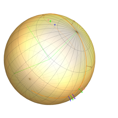
Figure 1: The fitted trajectory for $\alpha$ on the unit sphere

The fitted trajectory of $\alpha$ on the unit sphere is shown in Figure 1 and the dependence of $\theta$ and $R$ on $t=2\ln\left(\frac{\mu}{1\mathrm{Gev}}\right)$ are given in Figure 2 and Figure 3.

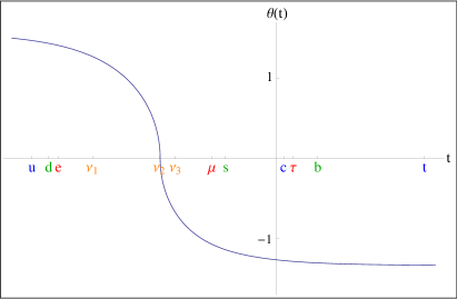
Figure 2: Fitted $\theta$ as a function of $t=2\ln\left(\frac{\mu}{1\mathrm{Gev}}\right)$

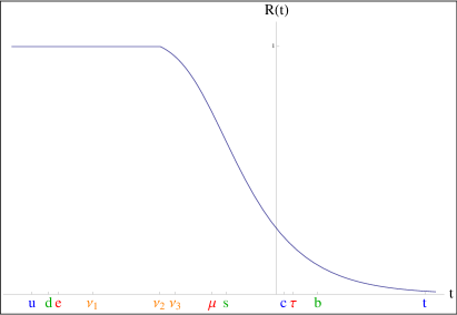
Figure 3: Fitted $R$ as a function of $t=2\ln\left(\frac{\mu}{1\mathrm{Gev}}\right)$

3 The vacuum transition at around 17 MeV

For this paper, what interests us in the above fit is the surprising fact that the FSM seems to have undergone a vacuum transition at a scale $\mu$ of around 17 MeV. One sees in Figures 2 and 3 that at some point, say $\mu_{T}\sim 17\ {\rm MeV}$, the derivative of $\theta$ with respect to $\mu$ becomes infinite while $R=1$ and remains at $1$ for $\mu<\mu_{T}$.

Now, the framon potential $V$ constructed, we recall, to be invariant under both the local symmetry $u(1)\times su(2)\times su(3)$ and the global symmetry $\tilde{u}(1)\times\widetilde{su}(2)\times\widetilde{su}(3)$ as the FSM requires, allows both the following 2 classes of vacua as minima of $V$, one class with $R$ varying with changing $\alpha$, and another class with $R=1$ and only $\alpha$ varying [25]. The above then seems to say that as the scale lowers from high values where the vacuum is originally of the first class, there will come a point, say $\mu=\mu_{T}\sim 17\ {\rm MeV}$, where a transition will occur when the vacuum moves into the other class where $R$ takes the fixed value $1$.

This transition, say VTR1, was first found in numerical solutions of the 2 coupled equations (12) and (13) while effecting the fit, but can be seen also analytically from the 2 equations, as will be detailed in the Appendix. It is also shown in the Appendix that the occurence of such a transition may not be restricted to the one-loop level at which the analysis has so far been carried out in detail, but seems to be kinematic in origin and may extend to higher loops. The value $\mu_{T}$ at which the transition occurs will change with more loops, as will indeed the whole fit performed in [10], but the occurence of such a transition seems likely to remain. It has to be said though that neither the mathematical structure nor the physical significance of VTR1 has yet been fully understood.

Notice that, as is shown in the Appendix, this vacuum transition need not always appear in the form selected in [10], but depends on the direction on the $\theta-R$ plane in which the transition point is approached. However, that the fit to data in [10] should choose to approach VTR1 in the direction indicated in the analysis above is no mystery. It was known already in R2M2 days [23] that in order to fit data the trajectory for $\alpha$ has to rotate at progressively greater speed as the scale $\mu$ decreases. In this type of models, as now in FSM, the lower generations acquire masses and the mixing matrices acquire nonzero mixing only by virtue of the rotation of $\alpha$, and the larger the values for the mass ratios, say $m_{c}/m_{t},m_{\mu}/m_{\tau}$, or the mixing matrix elements, say $V_{cb},U_{\mu 3}$, the faster the rotation will have to be. Given then the empirical values:

$$m_{c}/m_{t}\sim 0.007,\ \ m_{\mu}/m_{\tau}\sim 0.06;\ \ |V_{cb}|\sim 0.04,\ \ |U_{\mu 3}|\sim 0.73,$$ (16)

it follows that the curve of $\theta$ against $\mu$ in Figure 2 has to grow progressively steeper as $\mu$ decreases, as is seen to be indeed the case in the fit.

That the curve has to grow progressively steeper as the scale lowers does favour its approach to VTR1 in the direction it did, but cannot be taken as evidence that it should eventually acquire an infinite slope, namely that the transition VTR1 does indeed exist. Can one find other empirical facts to support this latter claim? The following two points are worth mentioning.

• [E1] First, empirically, from analyses in the SM, one wants $m_{u}<m_{d}$. This is a bit of a puzzle because $m_{t}>m_{b}$, $m_{c}>m_{s}$, namely the U-type is heavier than the D-type in the 2 higher (that is, heavier) generations, but only $m_{u}<m_{d}$ in the lowest (that is, the lightest) generation. Why? The R2M2 type of models for quark masses did not solve the puzzle for, as explained above, the masses of the lower generations come, according to these models, from “leakage” from the highest generation via the rotation of $\alpha$. Hence, the heavier the highest generation, the bigger will be the “leak” to the generations below, as confirmed by $m_{t}>m_{b}$, $m_{c}>m_{s}$. But why $m_{u}<m_{d}$? It was only in [10] that we have for the first time chanced upon an answer for this puzzle in the FSM framework, and it comes about in the following fashion. It was noted already some years ago [26] that for the R2M2 type of models it is the geodesic curvature of the rotation trajectory of $\alpha$ that governs the lowest generation mass. Now in the trajectory given by the fit of [10], as shown in Figure 1, the geodesic curvature changes sign when $\alpha$ passes through the transition point VTR1. And this, as explained in detail in [10], was what gave in that fit the very gratifying result $m_{u}<m_{d}$. And this can be claimed, at least within the FSM framework, to be a consequence of the VTR1 transition. We do not know, of course, whether $m_{u}<m_{d}$ has anything to do with $m_{p}<m_{n}$, the problem being nonperturbative is yet unsolved. But if it does, then we might have here even an answer to an ancient question so crucial to our own existence.

• [E2] The mass spectrum of the $H$ and $G$ states in the hidden sector [HS] mentioned above can and has been calculated in [16] where it is shown that there is a bunch of states with mass eigenvalues $\zeta_{S}\sqrt{{\textstyle{{1}\over{3}}}(1-R)}$, where $\zeta_{S}$, we recall, is a measure of the vacuum expectation value of the colour framon $\Phi$ with an estimated value of about 2 TeV. The physical masses of such states are to be measured by convention at the scale equal to their mass values, that is, solutions to the equation:

  $$\mu=\zeta_{S}\sqrt{{\textstyle{{1}\over{3}}}(1-R(\mu))}.$$ (17)

  Hence, given that $(1-R)$ is supposed to vanish at VTR1 at around 17 MeV, these states must have a solution to (17) for their physical mass just above but very close to 17 MeV. Two of these states, one scalar called $H_{+}$ and one vector called $G_{3}$, are known to have small couplings via mixing to our standard sector. The first can be made to accommodate the $g-2$ anomaly detected first some years ago at Brookhaven [27] and confirmed, up to a point, two years ago at Fermilab [28], while the second can be made to accommodate the so-called Atomki anomaly detected in excited ${}^{8}Be$ decay by [29], as was shown in [15].

The first piece of evidence [E1] is, of course, empirically solid but its relationship to VTR1 is not direct, while the relationship of the second piece [E2] to VTR1 is direct, but the empirical facts as well as their FSM interpretations have yet to be further justified.

In brief, although in the FSM framework the transition VTR1 is strongly indicated by the mass and mixing patterns of quarks and leptons, one has as yet understood in depth and detail neither its mathematical structure nor its physical significance. Nor has one gathered phenomenologically sufficient solid evidences as yet for its support. However, this vacuum transition, if it indeed exists, would have potentially, we believe, such a significance with such far-reaching physical consequences that it is worth being brought to the notice of the community even at this early stage of our own understanding of it.

In view of the importance of VTR1 to what follows, it would be useful to have an estimate of the error on the transition scale given above as 17 MeV. This, unfortunately, we are unable to provide, because the fit given in [10] was only the best we could find by trial and error. That we had chosen to proceed in such an ad hoc manner was not just negligence, there being a difficulty that we did not know how to overcome. What we wanted was an overall description of the whole mass and mixing pattern of quarks of leptons, using all the data then available, but the different bits of data came with widely varying accuracy, with,for example, the electron mass known to $10^{-8}$, while for the lepton mixing angle $\sin\theta_{23}$ only a bound was known, so that a $\chi^{2}$ fit would make little sense without weighting and any weighting made would be arbitrary. But if we allow ourselves to venture a guess, then from past experience and later applications [31], we would suggest as an estimate of the error on the transition scale of about 1—2 MeV. The reason for such a small-seeming error is the steepness of the curve for $\theta$ in Figure 2 near VTR1, so that a small change in $\mu$ would already make a big difference. That is, of course, if we keep narrowly within the present FSM framework.

We note in passing that although the exsistence of a vacuum transition at 17 MeV appears here as specific to the FSM via fitting to mass and mixing data, that there should be a new physical scale of that order was deduced by Bjorken [24] (7 MeV for him instead of 17 MeV here) via a line of dimensional arguments suggested by Zeldovich, and ultimately by Dirac, on much more general grounds.

4 Implied metric in the hidden sector

Our appreciation of the significance of the VTR1 transition is enhanced when considered in conjunction with the following facts.

The vierbeins in gravity are associated with a metric. The framons in FSM, or at least their vev’s, are supposed to be frame vectors too, like the vierbeins, and so should be associated with a metric as well. In that case, at VTR1 when $Q$ vanishes, that metric may develop singularities and it would be interesting to find out what would ensue. But first, of course, we have to clarify what is the metric implied by the framon vev’s and what it measures.

Let us turn back and recall where this $\mbox{\boldmath$\Phi$}_{\mathrm{\scriptscriptstyle{VAC}}}$ actually turned up in FSM calculations. It appeared in, for example, the Yukawa couplings, say (69) of [16], in the combination:

$$\mbox{\boldmath$\Phi$}_{\mathrm{\scriptscriptstyle{VAC}}}^{\dagger}\psi_{L}({\textstyle{{1}\over{6}}},2,3)=\chi_{L}({\textstyle{{1}\over{2}}},2,1),$$ (18)

where the numbers in brackets denote, respectively, the $U(1)$ charge, the dimension of the flavour representation, and the dimension of the colour representation. This is one of the $F$’s in the hidden sector [HS], being a colour-neutral bound state via colour confinement of the colour framon $\Phi$, a colour triplet, with the fundamental fermion $\psi_{L}({\textstyle{{1}\over{6}}},2,3)$, with the result still carrying the local flavour of the latter. It was called a co-quark, being the parallel of a quark in the standard sector, only with the roles of flavour and colour interchanged.

Now this $\chi_{L}$ is a vector in $\widetilde{su}(3)$ labelled by $\tilde{a}$ indices. Suppose we ask how this vector is to be normalized. To answer this, we first recall that $\psi_{L}$ in $su(3)$ colour is normalized thus:

$$\psi_{L}^{\dagger}\psi_{L}=1.$$ (19)

That being the case, then for the vector $\chi_{L}$ in dual colour $\widetilde{su}(3)$, just summing over the dual colour indices $\tilde{a}$ will not give us the norm, for according to (18), this will give us:

$$\chi_{L}^{\dagger}\chi_{L}=\zeta_{S}^{2}[Q^{2}\psi_{L1}^{*}\psi_{L1}+Q^{2}\psi_{L2}^{*}\psi_{L2}+P^{2}\psi_{L3}^{*}\psi_{L3}]$$ (20)

which is not unity. However, if we introduce a metric, say,

$${\bf G}=\zeta_{S}^{-2}\left(g^{\tilde{a}\tilde{b}}\right)=\zeta_{S}^{-2}{\rm diag}\,[Q^{-2},Q^{-2},P^{-2}],$$ (21)

then

$$|\chi_{L}|^{2}=\sum_{\tilde{a}\tilde{b}}\chi_{L\tilde{a}}^{\dagger}g^{\tilde{a}\tilde{b}}\chi_{L\tilde{b}}=|\psi_{L}|^{2}=1.$$ (22)

It is here, then, that the metric associated with $\mbox{\boldmath$\Phi$}_{\mathrm{\scriptscriptstyle{VAC}}}$ comes in, namely to give the norms for the state vectors $\chi_{L}$ in the dual colour representation.

We notice that, contrary to the vierbeins in gravity where it is the global reference metric that is orthonormal (that is, Minkowskian) while the local metric is distorted, here it is the metric of the local (that is, dependent on space-time point $x$) symmetry which remains orthonormal while it is the global (independent of space-time point $x$) reference metric that is being distorted as per (21) above. This is dictated by our requirement that local colour is confining so that its symmetry has to remain exact.

Although worked out specifically only for the co-quark (18) above, the same analysis clearly applies to all the $F$s, namely all co-quarks and co-leptons, formed as bound states of the colour framon with fundamental fermion fields. Their wave functions have all to be normalized with the metric (21).

Indeed, the same assertion holds also for all the other particles in the hidden sector, namely vector and scalar states $G$ and $H$ formed by colour confinement from framon-antiframon pairs. Let us work it out first for the $G$s which, in ’t Hooft’s confinement picture, are $p$-wave bound states of framon-antiframon pairs:

$$G_{\mu}=\mbox{\boldmath$\Phi$}^{\dagger}D_{\mu}\mbox{\boldmath$\Phi$}.$$ (23)

To leading order:

$$G_{\mu} = \mbox{\boldmath$\Phi$}_{\mathrm{\scriptscriptstyle{VAC}}}^{\dagger}\Omega^{-1}D_{\mu}\Omega\mbox{\boldmath$\Phi$}_{\mathrm{\scriptscriptstyle{VAC}}}$$ (24)

$$= \zeta_{S}\left(\begin{array}[]{ccc}Q&0&0\\ 0&Q&0\\ 0&0&P\end{array}\right)\tilde{C}_{\mu}\zeta_{S}\left(\begin{array}[]{ccc}Q&0&0\\ 0&Q&0\\ 0&0&P\end{array}\right).$$ (31)

where:

$$\tilde{C}_{\mu}=\Omega^{-1}D_{\mu}\Omega$$ (32)

is just a gauge transform of $C_{\mu}$ with $\Omega$ being the gauge rotation transforming from the standard gauge where the vacuum takes the form (8) to a general local colour gauge.

Now, for the colour gauge potential:

$$C_{\mu}=\sum_{K}C_{\mu}^{K}\lambda_{K},$$ (33)

we can define the norm as (using the usual normalization for the lambda matrices):

$$\|C_{\mu}\|^{2}={\textstyle{{1}\over{2}}}\mathop{\rm Tr}\nolimits[C_{\mu}^{\dagger}C^{\mu}]=\sum_{K}C_{\mu}^{K\dagger}C^{\mu K}.$$ (34)

Expanding similarly $\tilde{C}_{\mu}$ in (31) above, one has:

$$G_{\mu}=\mbox{\boldmath$\Phi$}_{\mathrm{\scriptscriptstyle{VAC}}}\sum_{K}\tilde{C}_{\mu}^{K}\lambda_{K}\mbox{\boldmath$\Phi$}_{\mathrm{\scriptscriptstyle{VAC}}}.$$ (35)

One sees then that it will not do to take the norm of $G_{\mu}$ just as $\mathop{\rm Tr}\nolimits[G_{\mu}^{\dagger}G^{\mu}]$. One should instead insert the metric (21) when summing over tilde indices, thus:

$$\|G_{\mu}\|^{2} = \mathop{\rm Tr}\nolimits[\mbox{\bf G}G_{\mu}^{\dagger}\mbox{\bf G}G^{\mu}]$$

$$= \mathop{\rm Tr}\nolimits[\mbox{\bf G}\mbox{\boldmath$\Phi$}_{\mathrm{\scriptscriptstyle{VAC}}}\sum_{K}\tilde{C}_{\mu}^{K\dagger}\lambda_{K}\mbox{\boldmath$\Phi$}_{\mathrm{\scriptscriptstyle{VAC}}}\mbox{\bf G}\mbox{\boldmath$\Phi$}_{\mathrm{\scriptscriptstyle{VAC}}}\sum_{L}\tilde{C}^{\mu L}\lambda_{L}\mbox{\boldmath$\Phi$}_{\mathrm{\scriptscriptstyle{VAC}}}]$$

$$= \mathop{\rm Tr}\nolimits[\mbox{\boldmath$\Phi$}_{\mathrm{\scriptscriptstyle{VAC}}}\mbox{\bf G}\mbox{\boldmath$\Phi$}_{\mathrm{\scriptscriptstyle{VAC}}}\sum_{K,L}\tilde{C}_{\mu}^{K\dagger}\lambda_{K}\mbox{\boldmath$\Phi$}_{\mathrm{\scriptscriptstyle{VAC}}}\mbox{\bf G}\mbox{\boldmath$\Phi$}_{\mathrm{\scriptscriptstyle{VAC}}}\tilde{C}^{\mu L}\lambda_{L}]$$

$$= \sum_{K}\tilde{C}_{\mu}^{K\dagger}\tilde{C}^{\mu K},$$

as claimed above, where in the last equality one has used the fact that:

$$\mbox{\boldmath$\Phi$}_{\mathrm{\scriptscriptstyle{VAC}}}\mbox{\bf G}\mbox{\boldmath$\Phi$}_{\mathrm{\scriptscriptstyle{VAC}}}=1.$$ (37)

The same is true also for the $H$ states which in ’t Hooft’s language are $s$-wave bound states of the colour framon with its conjugate via colour confinement, thus $\mbox{\boldmath$\Phi$}^{\dagger}\mbox{\boldmath$\Phi$}$. But, since $\Phi$ has nonzero vev, it is the fluctuations about $\mbox{\boldmath$\Phi$}_{\mathrm{\scriptscriptstyle{VAC}}}$ that counts as the $H$s, thus $\mbox{\boldmath$\Phi$}_{\mathrm{\scriptscriptstyle{VAC}}}\delta\mbox{\boldmath$\Phi$}$. Expanding then, one has:

$$\delta\mbox{\boldmath$\Phi$}=\left[\sum_{L=0,...,8}c_{L}\lambda_{L}\right]\mbox{\boldmath$\Phi$}_{\mathrm{\scriptscriptstyle{VAC}}},$$ (38)

where $\lambda_{0}=I/\sqrt{3}$. Notice that since the $H$s are in $s$-wave, the expansion is in the hermitian basis $\lambda_{L}$, not the anti-hermitian basis $i\lambda_{K}$ for the $p$-wave states $G$. Further, in our adopted notation, $\Phi$, hence also $\delta\mbox{\boldmath$\Phi$}$ and $\mbox{\boldmath$\Phi$}_{\mathrm{\scriptscriptstyle{VAC}}}$, are matrices whose rows are labelled by colour and columns by dual colour, while $\lambda_{L}$ and $\lambda_{K}$ are matrices whose rows and columns are both labelled by colour. This gives the $H$ states. in parallel to (35) for $G$, as:

$$H=\sum_{L}c_{L}\mbox{\boldmath$\Phi$}_{\mathrm{\scriptscriptstyle{VAC}}}\lambda_{L}\mbox{\boldmath$\Phi$}_{\mathrm{\scriptscriptstyle{VAC}}},$$ (39)

where we recall from (8) that $\mbox{\boldmath$\Phi$}_{\mathrm{\scriptscriptstyle{VAC}}}$ is a diagonal matrix with unequal diagonal elements. Hence, as for $G$, the norm of $H$ is not given just by $\mathop{\rm Tr}\nolimits[H^{\dagger}H]$ but by:

$$\|H\|^{2} = \mathop{\rm Tr}\nolimits[\mbox{\bf G}H^{\dagger}\mbox{\bf G}H]$$

$$= \sum_{L}|c_{L}|^{2}.$$

It appears then that the metric (21) applies to all particles $F,G,H$ comprising the hidden sector ${\bf[HS]}$ of the FSM when evaluating norms of their state vectors. Recall now that as the scale lowers towards VTR1, $R\rightarrow 1$, and 2 entries in (21) blow up, although since the corresponding components in the relevant state vectors vanish, there are no actual infinities in the norms. Nevertheless, this behaviour of the metric at VTR1 seems likely to have significant effects on the physics in the hidden sector where it operates. Our knowledge and understanding of the hidden sector being so meagre at present, our imagination has so far failed us in finding detectable effects therein, but we have noted already two interesting reflections [E1], [E2] they have on the standard sector. In any case, since the dynamics of the hidden and standard sectors are intimately connected, the noted singularity at VTR1 in the metric (21) in the hidden sector does not concern just that sector alone but could have grave repercussions on the whole scheme and has thus to be understood.

5 Kaluza-Klein embedding

Having failed so far in finding a verifiable effect of the transition VTR1 in the hidden sector itself, yet still wanting to find an example of such, we have then let our imagination loose, and it flew off at a tangent in the following direction. In gravity the vierbeins lead not just to a metric measuring the norms of vectors but to an actual metric of space-time itself. Attempting to mimic that, we try to imagine the whole FSM scheme being embedded, in Kaluza-Klein (KK) fashion, into a higher-dimensional space-time, a scheme we may call KFSM for short. In that case, we imagine, the vacuum transition VTR1 might lead to unusual behaviour of the metric in space-time itself and give rise to observable cosmological effects.

Before pushing further, however, two remarks are here appropriate. First, in making the KK assumption suggested above, one has gone beyond the original remits of the FSM. Hence, whatever new results one will obtain in this new venture, whether good or bad, should not affect the results obtained before with the FSM for particle physics to which it has so far been limited. And, of course, nor can the FSM alone claim credit for whatever the new venture might hope to achieve.

Secondly, we recognize, of course, that even the embedding of the SM into a KK theory is a sophisticated topic in itself already worked on by many eminent physicists without so far a definitive solution, and we have nothing to add to that. The embedding of the FSM into KK is therefore even more of an open problem and may not even be possible. We shall show, however, that so long as the KK embedding somehow goes through, what concern us in what follows are just a few compactified dimensions picked out by framing in the FSM as requiring our special attention, and so may not depend on details of how the KK embedding is actually effected.

With these reservations understood, let us then embark on our new adventure into the unknown, and prepare ourselves for confrontation with some unexpected consequences.

In a Kaluza-Klein theory, the compactified dimensions representing the gauged internal symmetry are generally supposed to be small in size so as to have escaped present detection, but it is usually not specified what actual sizes they do have. For example, some would suggest the Planck length. However, when the gauge theory involved is framed, as what interests us here, two significant changes ensue:

• The framons, though frame vectors in internal symmetry space, are Lorentz scalars in ordinary 4-dimensional space-time and so, as such, may acquire non-zero vacuum expectation values depending on their self-interaction potential.

• And, being frame vectors in internal space, those framons with non-zero vev’s would imply non-zero components of the metric, each of a certain size prescribed by the self-interaction potential in some specified direction of the compactified space representing the internal symmetry.

In other words, when the gauge theory embedded in the Kaluza-Klein scenario is framed, the physical concept of length is introduced into the compactified dimensions which they did not seem to have possessed before. One is then not free to assign arbitrary small sizes to all the compactified dimensions. Some of them will have to acquire the nonzero physical sizes specified and assigned to them by the framon self-interacting potential. We shall refer to these latter as the vev-enhanced dimensions, as opposed to those remaining dimensions corresponding to framon components with zero vev’s with therefore presumably still their original minimal size.

Specialize now to the FSM where the SM gauge symmetry is $G=u(1)\times su(2)\times su(3)$ and the flavour and colour symmetries are framed. In the confinement picture of ’t Hooft which the FSM has adopted and extended, both the global flavour and colour symmetries are broken and both the flavour and colour framons acquire non-zero vev’s. Let us first work it out for colour, which is of special interest to us here. For this, as already shown above, the framon has the vev (8), and this has led to the metric (21) for measuring lengths of vectors in the hidden sector.

Notice that $Q$ and $P$ are dimensionless but $\zeta_{S}^{-1}$ has the physical dimension $L$ of length. Hence (21) means that when applied to vectors in the colour symmetry space, which has initially no physical dimension, they will now acquire a norm with the physical dimension of length. Equivalently, which may be more convenient, one can shift the physical dimension to the vectors, saying that they are measured in units of $\zeta_{S}^{-1}$ with dimension $L$, and that their norms are to be defined with the dimensionless metric:

$$\hat{\bf g}=(g^{\tilde{a}\tilde{b}})=\left(\begin{array}[]{ccc}Q^{-2}&0&0\\ 0&Q^{-2}&0\\ 0&0&P^{-2}\end{array}\right).$$ (41)

Imagine next that there is a field of such vectors over those compactified dimensions which correspond to colour in the Kaluza-Klein scenario, and that this metric measuring the norms of these vectors is then to be taken as the contravariant metric. To this, the covariant metric measuring distance in the underlying Kaluza-Klein space would be the inverse:

$$\check{\bf g}=(g_{\tilde{a}\tilde{b}})=\left(\begin{array}[]{ccc}Q^{2}&0&0\\ 0&Q^{2}&0\\ 0&0&P^{2}\end{array}\right),$$ (42)

giving in those dimensions of the KK space the elemental distance $d\mbox{\boldmath$\sigma$}$ as:

$$d\mbox{\boldmath$\sigma$}^{2}=g_{\tilde{a}\tilde{b}}dx^{\tilde{a}}dx^{\tilde{b}}.$$ (43)

This metric (42) is also dimensionless, in keeping with the convention adopted above for (41). What is the physical dimension then of $d\mbox{\boldmath$\sigma$}$?

This distance $d\mbox{\boldmath$\sigma$}$ is measured in the manifold of compactified dimensions corresponding to colour in the Kaluza-Klein space while the vectors with norms of the dimension of length $L$ above live in the tangent space to this manifold, but locally, the tangent space and the manifold coincide. It seems thus natural that the line element $d\mbox{\boldmath$\sigma$}$ should have the same physical dimension as that of the vectors above, namely $L$ also. This means that, since we have adopted the covention that both the metrics (41) and (42) are dimensionless, it is the displacements in co-ordinates $dx^{\tilde{a}}$ which should carry this physical dimension $L$. This is exactly what is needed if these are to be taken as compactified dimensions of space as KK suggest.

This last assertion is by itself quite intriguing. In an ordinary KK theory when a gauge symmetry is embedded as extra dimensions in space-time, the symmetry space has in itself no physical dimension. But if it were to play the role of compactified dimensions in space as KK suggests, then it has to be given the physical dimension of $L^{d}$, where $d$ is the number of the extra dimensions introduced. Usually in the literature, as already noted above, this needed physical dimension is introduced via the Planck constant, tacitly thus assuming that the compactified dimensions are of the order of the Planck length in size. Here, we seem to be saying that in FSM, because the gauge symmetry is framed and its global dual is broken, some dimensions in that symmetry space get given not only a size but a size in the appropriate dimension of length $L$, and this size is of order $\zeta_{S}^{-1}$, with $\zeta_{S}$ being the strength of the vacuum expectation value of the framon field, which is much larger than the Planck length. That such a result should obtain in the FSM is traced to the confinement picture of ’t Hooft (extended to include colour) which gives the state vector of a co-quark as $\chi_{L}$ in (18), namely as a bound state of the fundamental fermion field with a framon, thereby making it carry the physical dimension of the latter.

Explicitly then, from (43) and (42), we have:

$$d\mbox{\boldmath$\sigma$}^{2}=Q^{2}(dx^{\tilde{1}})^{2}+Q^{2}(dx^{\tilde{2}})^{2}+P^{2}(dx^{\tilde{3}})^{2},$$ (44)

in the local $su(3)$ gauge where the framon $\Phi$ is hermitian and the global $\widetilde{su}(3)$ gauge where $\alpha$ points in the $\tilde{3}$ direction. We note also that $Q$ and $P$, though dependent on the renormalization scales $\mu$, do not depend on the co-ordinates $x^{\tilde{a}}$. This metric then signifies a 3-torus in space at every $\mu$.

This means then that of the compactified dimensions of the space representing the colour symmetry in the KK theory, those 3 denoted by the diagonal elements of $\check{\bf g}$ stand out as having acquired by symmetry-breaking a non-minimal size of order $\zeta_{S}^{-1}$, these forming together a 3-torus subspace of the colour symmetry space, while the other dimensions therein remain of the original minimal size.

A similar analyis can be carried out for the flavour symmetry [14, 16] which gives the line element in that subspace as:

$$d\sigma^{2}=\zeta_{W}^{-2}[{\textstyle{{1}\over{2}}}(dx^{\tilde{1}})^{2}+{\textstyle{{1}\over{2}}}(dx^{\tilde{2}})^{2}],$$ (45)

again signifying that of the several compactified dimensions of the space representing the flavour symmery in the KK theory, those 2 denoted by the diagonal elements of:

$$\check{\rm g}=\zeta_{W}^{-2}\,{\rm diag}\,[{\textstyle{{1}\over{2}}},{\textstyle{{1}\over{2}}}],$$ (46)

stand out as having acquired by symmetry-breaking a non-minimal size of order $\zeta_{W}^{-1}$ and form a 2-torus subspace of the flavour symmetry space, while the other dimensions remain of the original minimal size.

Altogether then, one seems to have acquired, by symmetry-breaking, 5 what we might call vev-enhanced dimensions of the internal symmetry space each with a size prescribed by the framon potential while the remaining dimensions of that space presumably would retain their original minimal size. And from the way this conclusion was worked out above, it seems that the world would look rather different to the standard or to the hidden sector particles.

To the standard sector particles such as the quarks, the leptons, the vector bosons $W-Z$ and the Higgs boson $h_{W}$, space-time would consist of (i) the usual 4 dimensions plus (ii) a vev-enhanced 2-torus of size of order $\zeta_{W}^{-1}$ as measured by the metric (46), plus (iii) some non-vev-enhanced dimensions with still unspecified minimal size corresponding to the remaining components of the flavour framon $\Phi$ with zero vev’s, while (iv) the colour dimensions and (v) the original $u(1)$ would appear in the usual Kaluza-Klein fashion as gauged symmetry spaces for colour and electromagnetism.

To the hidden sector particles $F$, $G$, and $H$, on the other hand, space-time would consist of (i) the usual 4 dimensions plus (ii) a vev-enhanced 3-torus of size of order $\zeta_{S}^{-1}$ as measured by the metric (42), plus (iii) the non-vev-enhanced dimensions with still unspecified minimal size corresponding to the remaining components of the colour framon with zero vev’s, while (iv) the flavour dimensions and (v) the original $u(1)$ would appear in usual Kaluza-Klein fashion as the gauged symmetry spaces for flavour and electromagnetism.

To the photon, however, which is in the FSM a mixture of a $u(1)$ gauged particle with the standard sector vector boson $Z$ and with a hidden sector vector boson $G$ [14, 16], the world will look again different in a way which will be of particular interest to us. To the photon, space-time would consist of (i) the usual 4 dimensions plus (ii) a 2-torus of size $\zeta_{W}^{-1}$ plus (iii) a 3-torus of size $\zeta_{S}^{-1}$ plus (iv) other compactified dimensions of minimal size, while (v) the original $U(1)$ dimension would remain in the KK fashion as the gauged symmetry space of electromagnetism.

Our next question is how this structure will change with changing scale. In particular, we are interested in how it would behave as $\mu$ approaches the VTR1 transition, say, from above. Now, of the many compactified dimensions with minimal sizes we know nothing, and can only assume that they remain more or less oblivious to such scale-changes. Of the 5 vev-enhanced dimensions, the 2 from flavour have a size proportional to $\zeta_{W}^{-1}$, where $\zeta_{W}\sim 246$ Gev and is known to be only weakly dependent on scale. But the remaining 3 from colour have different sizes: $\zeta_{S}^{-1}$ times $Q$ or $P$, as given in (10), where $R$ is known to be strongly scale-dependent, as seen in Figure 3. Indeed, as the scale approaches the vacuum transition VTR1 at around 17 MeV, we see that those 2 dimensions with size proportional to $Q$ would shrink to zero. This means that the volume of the whole 3-torus formed from the 3 vev-enhanced dimensions would collapse to zero altogether.

From the fit in [10] to the mass and mixing data of quarks and leptons, one has in FSM even a rough picture of how this collapse may behave as it nears the VTR1 transition point. According to the metric (42), the 3-torus in the vev-enhanced dimensions has a volume proportional to:

$$\zeta_{S}^{-3}(1-R)\sqrt{1+2R}.$$ (47)

The behaviour of $R$ near VTR1 is given in Figure 3, but there is as yet no direct information on $\zeta_{S}$ except for an estimated value of $\zeta_{S}\sim 2$ TeV at high scales (say around the top mass $m_{t}$) from [14]. However, we recall from (11) that:

$$\zeta_{S}^{-1}=\sqrt{R\frac{2\kappa}{\nu_{2}\zeta_{W}^{2}}}$$ (48)

where $\zeta_{W}$ is known to be about 246 GeV and weakly dependent on scale, while $\kappa$ and $\nu_{2}$ are dimensionless couplings in the framon potential (7) which are naturally of order unity and hence also likely to be weakly scale-dependent. Though crude, this last assertion is checked to be consistent with the above estimate of $\zeta_{S}\sim 2$ TeV at $\mu\sim m_{t}$ where $R\sim 0.01$. If so, then we have roughly that $\zeta_{S}^{-1}\sim\sqrt{R}$ in scale-dependence giving instead of (47):

$$R^{3/2}(1-R)\sqrt{1+2R},$$ (49)

for the scale-dependence of the volume of the vev-enhanced 3-torus in colour near the VTR1 transition. And, if we ignore the unkown scale-dependence of the non-vev-enhanced Planck sized dimensions, the same behaviour would apply to the whole compactified subspace corresponding to the colour symmetry in the KK scenario.

From Figure 3 then, one obtains via (49) Figure 4. The volume of the subspace corresponding to colour is seen to start off at high $\mu$ ($\sim m_{t}$) with a small value, rising at first as $\mu$ lowers, in line with the usual 3 dimensions of space, but then as the scale nears the VTR1 transition at $\mu_{T}\sim$ 17 MeV, it drops quite abruptly to zero.

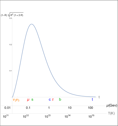
Figure 4: A sketch of how, as surmised, the volume of the compactified colour dimensions would vary with scale and shrink eventually to zero as the scale lowers towards the VTR1 transition.

In other words, the KFSM scheme seems to say that, driven by some microscopic dynamics mostly in the hidden sector, space-time in the Kaluza-Klein scenario would lose at VTR1 quite abruptly 2 of its compactified spatial dimensions. If this is true, dramatic effects, it seems, can hardly be avoided. In the next section, we aim to set our imagination loose and try to figure out how the evolution of the early universe might be affected—purely in a spirit of exploration on our part, however inadequately equipped we know we really are for the task.

6 Possible effect on the horizon problem

Suppose we accept the above picture of the FSM embedded Kaluza-Klein fashion into space-time, namely that space-time is effecively 10-dimensional: 4 for the usual, plus 1 compactified for the $u(1)$ gauge, plus 2 compactified vev-enhanced for flavour, plus further 3 compactified vev-enhanced for colour. The 2 vev-enhanced dimensions for flavour have a size of order $\zeta_{W}^{-1}$ where $\zeta_{W}$ is the vev of the standard Higgs field of order 246 GeV, while the 3 vev-enhanced dimensions for colour have sizes of order $\zeta_{S}^{-1}$ where $\zeta_{S}$ is the vev strength of the colour framon (a new ingredient of FSM with no analogue in the SM) thought to be of order TeV at high scales but probably quite strongly scale-dependent. There are other compactified dimensions with minimal sizes about which we know nothing and can and shall largely ignore. Let us accept also, as put forward above, that because of the vacuum transition VTR1 found in FSM at a scale of around 17 MeV [10], 2 of the 3 vev-enhanced dimensions for colour shrink to zero as the scale approaches VTR1 from above, as depicted in Figure 4.

Suppose further that as the universe cooled, it was its temperature at every stage which set the scale so that we can follow the development of VTR1 in Figure 4 just by converting the scale $\mu$ to the temperature $T$ as shown. One sees then that as the universe cooled from some initial high temperature, the compactified dimensions for colour first expanded, in line with the usual 3 space dimensions, but then started to contract when the transition VTR1 at a scale of about 17 MeV was approached. This corresponds to a temperature of about $2.0\times 10^{11}$ K when the universe was around $2.5\times 10^{-3}$ s old.

What would happen then at this transition when 2 of the compatified dimensions are supposed to shrink to zero? This reminds one of a balloon being squeezed—if compressed in one direction, it would expand in the other directions, as long as the amount of air it contains is kept the same. Would something similar occur to the early universe at VTR1?

It would seem that it might. The universe around the time of the VTR1 was radiation-dominated, so that in terms of the balloon analogy that we cavalierly suggested above, the air inside the balloon would here be replaced by black body radiation. This in a sense makes the problem easier, since the energy density per unit volume would, by Jean’s Law, be a function of just the temperature. In Figure 4 we saw that VTR1 is supposed to occur over a relatively short range of temperature. Suppose that as a first approximation we take the transition to be isothermal, then the energy density of the black body radiation contained would remain the same. And if the number of photons also remains the same, the volume they occupy should remain the same before and after the transition. Hence at VTR1, when 2 of the compactified dimensions shrink to zero, the other dimensions will have to expand to compensate, as envisaged in the balloon analogue.

In the present Kaluza-Klein scenario many dimensions are involved. Apart from the usual 4 dimensions of space-time, we have in addition the compactified dimensions corresponding to the embedded internal symmetry $G$. Hence, when 2 of the latter dimensions corresponding to colour are squeezed by VTR1 as proposed, we have to ask which of the remaining dimensions will expand to compensate. We recall first from (42) that when $R\rightarrow 1$ as VTR1 is approached and 2 diagonal entries in $\check{\bf g}$ shrink to zero, the third entry just goes gently to $1\times\zeta_{S}^{-2}$ and cannot expand. Neither can the compactified dimensions corresponding to flavour, the size of which were seen to be governed by $\zeta_{W}$, known in the standard electroweak theory to be only weakly scale-dependent. Of the compactified dimensions there remain then only the $u(1)$ gauge and the ones we labelled as non-vev-enhanced all of minimal Planck size which we have assumed, and shall continue to assume, to be oblivious to scale changes. In that case, it would seem that at VTR1 when the 2 collapsing dimensions shrink to zero, only the 3 standard spatial dimensons can freely expand to compensate for the shrinkage.

Supposing this is true, let us ask next by how much the 3 spatial dimensions might be expected to expand under VTR1. The 2 collapsing dimensions are supposed to have started just before the VTR1 with a value of order $\zeta_{S}^{-1}\sim\zeta_{W}^{-1}$. If they actually shrank to zero after VTR1, then the expansion of course would be infinite. Let us however take zero practically to mean only the smallest length known, namely the Planck length:

$$\ell_{Pl}=m_{Pl}^{-1}\sim 1.616\times 10^{-35}\ {\rm m},$$ (50)

then the expansion will be large, but finite.

Assuming next that the universe remained isotropic, for example with the Robertson-Walker metric [32, 33, 34, 35], and remaining still for the moment in the approximation when VTR1 is taken isothermal so that the volume remained the same before and after the transition, we will then have:

$${\cal R}_{F}^{3}\ell_{Pl}^{2}\sim{\cal R}_{I}^{3}{\ell_{I}}^{2},$$ (51)

where ${\cal R}_{I}$ is initial size of the universe before the VRT1 transition, ${\cal R}_{F}$ the expanded size after the transition, and $\ell_{I}$ is the initial size of the 2 compactified colour dimensions which were shrunk to the size of the Planck length by the transition.

Suppose we substitute then for $\ell_{I}$ the above order of magnitute estimate:

$$\ell_{I}\sim\zeta_{S}^{-1}(\mu\sim\mu_{T})\sim\zeta_{W}^{-1}\sim(246\ {\rm GeV})^{-1}\sim 8.0\times 10^{-19}\ {\rm m}.$$ (52)

We obtain the order of magnitude estimate for the expansion factor:

$${\cal E}_{\rm isotherm}=\frac{{\cal R}_{F}}{{\cal R}_{I}}\Bigg{|}_{\rm isotherm}$$ (53)

as:

$${\cal E}_{\rm isotherm}\sim\left(\frac{\ell_{I}}{\ell_{\rm Pl}}\right)^{2/3}=\left(\frac{8.0\times 10^{-19}}{1.6\times 10^{-35}}\right)^{2/3}=1.4\times 10^{11}.$$ (54)

That such an expansion would be enough to imply a universe smaller in size than the horizon before the transition can be seen as follows.

The portion of the universe that is observable to us, or in other words the horizon at present, is

$$t_{0}=1.38\times 10^{10}\ {\rm yr},$$ (55)

which in units of length is

$${\cal R}_{0}={\cal H}_{0}\sim 3t_{0}\sim 4.14\times 10^{10}\ {\rm ly}\sim 3.92\times 10^{26}\ {\rm m}.$$ (56)

For general time $t$, however, we need to distinguish between the two concepts: ${\cal R}$ the size of the universe, and ${\cal H}$ the horizon, since the two evolve with time differently.

Tracing the evolution backwards in the standard Big Bang model, one estimates that the part of the universe we now observe, or the universe for short, was, at its age of $2.5\times 10^{-3}$ s just after the VTR1 transition, only about

$${\cal R}_{T+}\sim 3.7\times 10^{15}\ {\rm m}$$ (57)

in size. In arriving at this estimate, we have taken account of the knowledge [3, 4] that the energy density of the universe was dominated by matter from now at an age of $1.38\times 10^{10}$ yr back to about $4\times 10^{4}$ yr, when its size depended on time roughly as $t^{2/3}$, but from then onwards back to its age just after VTR1, when it was radiation dominated, and its size depended on time as $t^{1/2}$.

On the other hand, the horizon ${\cal H}$ depended on time roughly as $2t$ when the universe was radiation dominated, so that at the time around VTR1, when its age was $\sim 2.5\times 10^{-3}\ {\rm s}$, the horizon was only of order:

$${\cal H}_{\rm VT}\sim 1.5\times 10^{6}\ {\rm m}.$$ (58)

In other words, the universe then of size (57), as estimated above, was made up of numerous causally disconnected bits, as it was already at the decoupling time when the CMB was formed, only exacerbated.

However, given the size of the universe ${\cal R}_{T+}$ in (57) just after the transition and the estimate (54) for the expansion factor due to VTR1, one concludes that the universe would have expanded from a size ${\cal R}_{T-}$ just before the transition of only:

$${\cal R}_{T-}\sim\frac{3.7\times 10^{15}\ {\rm m}}{1.4\times 10^{11}}\sim 2.7\times 10^{4}\ {\rm m},$$ (59)

which would fit comfortably inside the horizon at that time, namely the ratio of size to horizon:

$$\frac{{\cal R}}{{\cal H}}\Bigg{|}_{T=17\ {\rm MeV}}\sim 0.018;\ \ \ {\rm isothermal\ approx.}$$ (60)

This estimate is inaccurate, however, having been derived assuming that the VTR1 transition is isothermal, which it clearly is not. As seen in Figure 4, it seems to have occurred over a period corresponding to about half-a-decade drop in temperature, say from about 100 MeV to 17 MeV. Recalling that the energy density of black body radiation depends on temperature as $T^{4}$ (the Stefan–Boltzmann Law), we can correct roughly for the drop in temperature by multiplying (54) by the factor $(T_{F}/T_{I})^{4/3}$ which for $T_{I}\sim 100\ {\rm MeV},T_{F}\sim 17\ {\rm MeV}$ gives a value of $\sim(17/100)^{1.33}\sim 0.095$, hence for the corrected expansion factor ${\cal E}$:

$${\cal E}_{\rm temp.\ corr.}=\frac{{\cal R}_{F}}{{\cal R}_{I}}\sim 1.3\times 10^{10},$$ (61)

or that the initial size of the universe before the VTR1 expansion as:

$${\cal R}_{I}\sim 2.87\times 10^{5}\ {\rm m},$$ (62)

and for the ratio of size to horizon:

$$\frac{{\cal R}}{{\cal H}}\Bigg{|}_{T=17\ {\rm MeV}}\sim 0.19;\ \ \ {\rm temp.\ corr.},$$ (63)

leaving the universe still lying inside the horizon.

But this is about the best that we can do at present to correct for the isothermal approximation made, without further knowledge of the physics governing the universe in the earlier epoch at temperatures above the VTR1 transition. Ideally, one should have followed the development of the universe as it evolved in time towards the VTR1 transition to evaluate properly the expansion factor ${\cal E}$ one needs, but this is not possible, at least for us, when even the Kaluza-Klein theory supposed to govern that evolution is not fully spelt out.

Given these very approximate numbers and the fact that they are, in the first place, meant to be just order of magnitude estimates, one can only say that:

• [C] The expansion due to the vacuum transition VTR1 in FSM is of an order of magnitude capable of taking a universe inside the horizon at some time before, to a size of the order of a light year at time $T_{+}$ just after, which will then further evolve by Hubble expansion to our universe today, of which all portions would then have, at one stage, been causally connected.

But even so, it would seem that one has here on offer a possible answer to the immediate question posed by the horizon problem.

To qualify, however, as a serious candidate solution of the problem, it has yet to be ensured that the above scenario is not inconsistent with other known properties of the universe, and this has not been done. There are questions that we have heard about but cannot as yet answer, such as the flatness problem, the problem of large scale inhomogeneities and so on, which the VTR1 transition might affect. There are probably many other questions (for example the entropy paradox [36]) that we are insufficiently knowledgeable even to ask, let alone answer. The purpose here is therefore not to claim a new solution of the horizon problem but merely to make known a suggestive observation from the angle of particle physics in the hope that experts in cosmology and the early universe might wish to consider.

But if, at this low level of plausibility, the above VTR1 scenario is taken as a candidate solution to the horizon problem, then it would have in addition the following seemingly attractive features:

• It is not constructed specifically to solve the horizon problem but a consequence of the FSM constructed for particle physics, apart of course from the Kaluza-Klein embedding which is what connects it to cosmology. Even the values of all the parameters which entered in the above discussion came from fits to particle physics data and none has been adjusted in this paper to arrive at the stated results.

• The VTR1, being driven in the FSM by the underlying microscopic particle physics, would turn itself on and off automatically as the universe cooled and, being in the FSM a global effect, it would do so simultaneuosly over all space .

• The present FSM fit to particle data says that when $R$ reaches the value 1 at VTR1, it will stay there ever afterwards, meaning that the expansion caused by VTR1 would be all over by $t\sim 2.5\times 10^{-3}$ s. It need not therefore affect previous successes of the Big Bang idea, such as that on nucleosynthesis, which occurred at much later times.

• The expansion caused by VTR1 being “quasi-isothermal” and even during that short time when it operated it is supposed to incur no more than the usual cooling of the universe, no reheating would seem to be required. Indeed, since the overall (multidimensional) volume is supposed to remain almost the same, the transition can be interpreted less as an expansion than as a mere change of shape.

7 Concluding Remark

The observation of the preceding section on the horizon problem, though exciting it can be, is only speculative, depending as it does on the Kaluza–Klein assumption, which, as far as we know has so far no empirical justification, and involving also some steps which can do with much closer scrutiny. Nevertheless, it serves as an indication of what powerful effects the VTR1 transition can have on the dynamics of the hidden sector. Now in the FSM, a peculiar fact is that although the hidden and standard sectors have little direct interactions with one another, their dynamics are nevertheless intimately connected. For example, even the mass and mixing patterns of quarks and leptons, we recall from Section 2, are consequences of framon-loop renormalization in the hidden sector. Recall further that the hidden sector is in FSM potentially where the dark matter of the universe resides. It looks very likely, therefore, that the VTR1 would play a significant role in determining both the intrinsic properties of the underlying theory and the overall structure of the universe. Unfortunately, we have as yet no idea how to probe systematically these effects, or even what salient questions to ask, our knowledge of the hidden sector being at present so strictly limited. We can only hope that, with persistence and help from the community, something will eventually emerge to take us further on our way.  
 
Appendix  

What interests us in this appendix is the behaviour of the evolution equations (12) and (13) near $R=1$ where the vacuum transition VTR1 is seen to occur, as noted in the text. Our first concern is to check this conclusion analytically, to make sure that it is not just a fluke of the numerical solution. This would be prudent for there are zeros at the transition point both in the numerators and in the denominators on the right-hand side of the 2 equations, and the behaviour of the solution is the result of some delicate cancellations of these zeros against one another, which cancellatons can depend on the direction on the $R\theta$-plane in which the transition point is approached.

Before studying these cancellations in detail, let us first make clear that the curve traced out by $\alpha$ on the unit sphere is itself perfectly regular, with no singularities anywhere, in particular with nothing untoward happening at the pole. What might seem singular there arise only from the singularities in the polar coordinates themselves. That this is the case can be seen by casting the equation (14) which specifies this curve in terms of the Cartesian coordinates $\mbox{\boldmath$\alpha$}=(x,y,z)$, with $x^{2}+y^{2}+z^{2}=1$, thus:

$$yz/x=a.$$ (64)

This is the equation of a hyperbolic paraboloid, and it is its intersection with the unit sphere that gives the curve we want. We note that Figure 1 of [10] shows only part of this curve corresponding to different values of the parameter $a$, but the whole intersection is a closed curve, easily obtainable from that figure using the symmetries of (64). In the fitted trajectory in [10] (with $a=-0.1$), we stay in the upper hemisphere. This is clearly shown in Figure 5 there (the “back” view). Since we have chosen there $a$ to be negative, the curve stays in the fourth and second quadrant above the equatorial plane, and switches to the first and third quadrant below the equatorial plane. (This is the part not shown, not being needed there). One could have chosen $a$ to be positive, and it will be the other way round, but this is just a matter of choice, with no real significance.

Zooming in to the pole ($z=1$), where $y=-0.1x$, we note that the curve is tangent to this line through the pole, going from the fourth quadrant to the second quadrant in the northern hemisphere. It is also tangent to the geodesic (the great circle) through the pole with the same slope (if we look at the tangent plane there). This means the curve has zero geodesic curvature at the pole. The geodesic curvature changes sign as the curve goes through the pole, as can be seen pictorially in the figure, as a consequence of the symmetry under $(x,y)\leftrightarrow(-x,-y)$, or reflection with respect to the pole. As explained in [10], this change of sign of the geodesic curvature is significant in giving in FSM the physically crucial and theoretically intriguing result: $m_{u}<m_{d}$, despite the fact that the heavier generations appear in the opposite order: $m_{t}\gg m_{b},m_{c}\gg m_{s}$.

We have gone through the properties of the curve traced out by $\alpha$ in detail to highlight the fact that it is perfectly regular, with no singularity anywhere, so that the noted VTR1 transition at the pole must have originated from the equations (12) and (13) governing the speed at which $\alpha$ moves along that curve, and it is to these equations we now turn our attention.

We shall concentrate on the region around the pole, and expand around that point thus: $R=1-\delta_{1},\ \theta=\delta_{2}$, with both deltas small and positive, meaning that we are approaching that point from above in $\mu$. And we take $\delta_{1}$ and $\delta_{2}$ to be independent so as to study how the behaviour may change depending on the direction in which that point is approached on the $R\theta$-plane. This behaviour is found to depend crucially on the denominator $D$ (15) appearing in the equations:

$$D = R(1+2R)-3R\cos^{2}\theta+k(1-R)(1+2R)$$ (65)

$$= 2\delta_{1}+2\delta_{1}^{2}+3\delta_{2}^{2}+3k\delta_{1}-2k\delta_{1}^{2}+O(\delta^{3})$$

Expanding similarly the other quantities appearing in the equations, and ignoring some unimportant positive constant coefficents, we find that:

$$\dot{R} \sim -\frac{\delta_{1}(1-\delta_{1})(3-2\delta_{1})}{D}$$ (66)

$$\dot{\theta} \sim -\frac{2(1-\delta_{2})\delta_{2}}{D}$$ (67)

The following conclusion then results:

• (a) If $\delta_{1}\ll\delta_{2}^{2}$, then $\dot{R}\to 0,\dot{\theta}\to-\infty$.

• (b) If $\delta_{1}\sim\delta_{2}^{2}$, then $\dot{R}\to$ nonzero constant, $\dot{\theta}\to\infty$.

• (c) If $\delta_{1}\gg\delta_{2}^{2}$, then $\dot{R}\to$ nonzero constant, $\dot{\theta}\to 0$.

As expected, the behaviour of the trajectories for $R$ and $\theta$ at the transitional point depends crucially on the direction in which that point is approached on the $R\theta$-plane. This direction, however, is not free for us to choose but is determined by the initial condition in solving the equations, or in the case of [10] by the fit to the higher mass states above the transitional point. And this fit has chosen the case ${\bf(a)}$, as seen in Figure 2 by the steep approach of $\theta$ to the transition point as compared with the slow approach of $R$ seen in Figure 3. This means that the condition set out in (a) is satisfied and that $\dot{R}\rightarrow 0$ as the result, confirming thus the conclusion on VTR1 drawn from the numerical solution in [10]. Indeeed, it is fortunate for the FSM that it has made this choice (a), for the other two cases (b) and (c) are not physical in the model where $R\leq 1$ is required.

After going over the pole, the case (a) now being chosen, $\dot{R}=0$ and hence $R=1$ for the rest of the trajectory. This means that the tenets of the VTR1 transition first deduced from the numerical fit in [10] is analytically confirmed.

Indeed, that $\dot{R}=0,R=1$ allows also (13) to be analytically integrated and again confirms the numerical result obtained in [10], but as this concerns only such results as $m_{u}<m_{d}$ already mentioned, of interest elsewhere but not directly in the present VTR1 context, it need not be detailed here.

Next, knowing now that the VTR1 transition does indeed occur in the scenario described in [10], we ask whether this assertion is limited only to the 1-loop approximation studied there, or it is likely to persist in a more general situation. We intend to show in what follows that the latter is the case.

We note first that what the deduction of VTR1 in [10] relies on is the renormalization by a framon loop of a fermion mass matrix (not of the standard quarks and leptons but of some fermions in the hidden sector generically called $F$, as already mentioned in the text), but the evolution equation (RGE) derived on which the result is based concerns only a left-handed vector pertaining to that mass matrix, given in [10] equation (32) as:

$$\frac{d}{dt}(\rho_{S}\zeta_{S}V_{0}\mbox{\bf v})=\left(\begin{array}[]{ccc}\gamma&0&0\\ 0&\gamma&0\\ 0&0&\beta\end{array}\right)(\rho_{S}\zeta_{S}V_{0}\mbox{\bf v}).$$ (68)

That an RGE for a matrix should end up only as an evolution equation for a vector comes about because the fermion mass matrix and the framon couplings renormalizing it in this model are all factorizable into a left-handed (ket) vector times a right-handed (bra) vector. And by the same token, it would remain the same no matter how many framon loops are inserted; the resulting RGE would be factorizable, resulting thus in just an evolution equation for a left-handed ket, as in (68).

Further, one notes that the evolution operator on the right of (68) is a diagonal matrix with its first two entries indentical. This comes about because the FSM has an inherent $su(2)$ symmetry between two of its framons, labelled here $\tilde{1}$ and $\tilde{2}$, although in [10] this was deduced by explicit calculation to 1-framon-loop order. When more framon loops are inserted, the said $su(2)$ symmetry is maintained. The evolution operator will have to be invariant under all $su(2)$ transformations of $\tilde{1},\tilde{2}$ so that, by Schur’s lemma, it would still have to be of the form shown, namely a diagonal matrix with two identical eigenvalues, although their values will no longer be the same as that given in [10] but would involve higher order terms.

Now in [10], from the fact that two eigenvalues of the evolution operator are identical follows a chain of deduction leading to the shape equation of the curve $\Gamma$. Thus, from (68) above, one has:

$$\frac{\dot{v_{2}}}{v_{2}}=\frac{\dot{v_{1}}}{v_{1}},$$ (69)

which gives:

$$v_{2}={\rm constant}\times v_{1},$$ (70)

and hence, via equation (39) there,

$$\frac{\alpha^{\tilde{2}}\alpha^{\tilde{2}}}{\alpha^{\tilde{1}}}={\rm constant},$$ (71)

This chain of deduction, relying only on the symmetry between $\tilde{1}$ and $\tilde{2}$ would still be valid even when these eigenvalues are modified by higher loops. This means that $\Gamma$ would remain the same in shape, having for example a change in sign of its geodesic curvature at $\theta=0$, and retaining thereby the result $m_{u}<m_{d}$ which we so coveted.

More critical for the occurence of the transition VTR1, however, are the equations (12) and (13). Examine first (12). The factor on the R.H.S. in front of the square bracket comes from the L.H.S. of the equation (68) and does not depend on the 1-loop calculation which affects only the R.H.S. of (68). Now, however, the analysis above in (65) to (67) of how $R$ behaves near the transition point relies only on this factor, not on the quantity inside the square bracket. Hence, even if we were to add higher loop terms inside the square bracket, the behaviour of $R$ would remain the same and lead to the conclusions (a) to (c) as listed before, in particular (a) under the same conditions. Namely, provided that the transition point is approached in such a way that $\delta_{1}\ll\delta_{2}^{2}$, then $\dot{R}\to 0,\dot{\theta}\to-\infty$.

Next, examine equation (13), or rather the equation (43) of [10] from which it is derived, namely:

$$\frac{\dot{\alpha}^{\tilde{3}}}{\alpha^{\tilde{3}}}=\beta-\frac{\dot{P}}{P}+\frac{k}{2}\frac{\dot{R}}{R}.$$ (72)

In terms of polar co-ordinates, this read as:

$$\dot{\theta}=-\frac{\cos\theta}{\sin\theta}\left[\beta+\dot{R}\left(-\frac{1}{1+2R}+\frac{k}{2R}\right)\right].$$ (73)

In these equations, all originating from (68), only $\beta$ comes from the R.H.S. of (68) which in the one-loop approximation is given in [10] but is the only quantity which will change when more loops are included. When the transition point is approached, as in case (a) above, $\dot{R}$ vanishes, so that $\dot{\theta}\rightarrow-\infty$ so long as $\beta$ is finite, which it is in the one-loop approximation and is unlikely to change when more loops are added.

We conclude therefore that the transition VTR1 is not limited to the one-loop appoximation but will persist when more loops are included. The actual formulae will differ from [10] and so will the details of the fit to data, such as the value of $\mu_{T}$ where the transition occurs. However, whatever new fit will have to respect the data and end up not very different from the picture shown. We suspect, therefore, that even the numerical result will not change much when more loops are included.

References

- [1] A. Friedmann, Z. Phys. 16, 377 (1922); doi:10.1007/BF01332580
- [2] A. Friedmann, Z. Phys. 21, 326 (1924); doi.org/10.1007/BF01328280
- [3] Steven Weinberg, Cosmology, Oxford University Press, 2008. ISBN: 9780198526827
- [4] P. A. Zyla et al., (Particle Data Group), Prog. Theor. Exp. Phys. 2020, 083C01 (2020); http://pdg.lbl.gov/
- [5] Christian Knobel, “An Introduction into the Theory of Cosmological Structure Formation”, doi:10.48550/arXiv.1208.5931; arXiv:1208.5931[astro-ph.CO]
- [6] A. Guth, Phys. Rev. D23, 347 (1981); doi:10.1103/PhysRevD.23.347
- [7] D. Linde, Phys. Lett. B108, 389 (1982); doi:10.1016/0370-2693(82)91219-9.
- [8] D. Linde, Phys. Rev. Lett. 48, 335 (1982); doi:10.1016/0370-2693(82)90293-3.
- [9] A. Albrecht and P. Steinhardt, Phys. Rev. Lett. 48, 1220 (1982); doi:10.1103/PhysRevLett.48.1437.
- [10] José Bordes, Chan Hong-Mo and Tsou Sheung Tsun, Int. J. Mod. Phys. A30 (2015) 1550051; doi:10.1142/S0217751X15500517; arXiv:1410.8022[hep-ph].
- [11] José Bordes, Chan Hong-Mo and Tsou Sheung Tsun, Int.J.Mod.Phys.A 36 (2021), 2150236; doi:10.1142/S0217751X21502365; arXiv:2107.05420[hep-ph].
- [12] José Bordes, Chan Hong-Mo and Tsou Sheung Tsun, Int. J. Mod. Phys. A36 (2021) 2150238; doi:10.1142/S0217751X21502389; arXiv:2109.11391[hep-ph].
- [13] José Bordes, Chan Hong-Mo and Tsou Sheung Tsun, Int. J. Mod. Phys. A37, No. 27, 2250167 (2022); doi:10.1142/S0217751X22501676; arXiv:2206.06687[hep-ph].
- [14] José Bordes, Chan Hong-Mo and Tsou Sheung Tsun, Int. J. Mod. Phys. A33 (2018), 1850190; doi:217751X18501907; arXiv:1806.08271[hep-ph].
- [15] José Bordes, Chan Hong-Mo and Tsou Sheung Tsun, Int. J. Mod. Phys. A34 (2019) 1950140; doi:10.1142/So217751X19501409; arXiv:1906.09229[hep-ph].
- [16] José Bordes, Chan Hong-Mo and Tsou Sheung Tsun, Int. J. Mod. Phys. A33 (2018) 1850195; doi:10.1142/S0217751X18501956; arXiv:1806.08268[hep-ph].
- [17] K. Abe et al. (T2K Collaboration), Nature, 580, 339-344 (2020); doi:10.1038/s41586-020-2177-0; arXiv:1910.03887[hep-ex].
- [18] T. Aaltonen et al. (CDF collaboration), Science 376, 170 (2022); doi:10.1126/science.abk1781.
- [19] A. Keshavarzi, D. Nomura and T. Teubner, Phys. Rev. D 97, 114025 (2018); doi:10.1103/PhysRevD.97.114025; arXiv:1802.02995[hep-ph].
- [20] Chan Hong-Mo and Tsou Sheung Tsun, Invited contribution, “A Festschrift in Honour of the CN Yang Centenary”. Edited F. C. Chen et al., 2022 (World Scientific); doi:10.48550/arXiv.2201.12256; arXiv:2201.12256[hep-ph].
- [21] G. ’t Hooft, Acta Phys. Austr., Suppl. 22, 531 (1980);
- [22] G. ’t Hooft, “Topological aspects of Quantum Chromodynamics”, Erice Lecture notes, August/September 1998. arXiv:hep-th/9812204.
- [23] Michael J Baker, José Bordes, Chan Hong-Mo and Tsou Sheung Tsun, Int. J. Mod. Phys. A26 (2011) 2087-2124; doi: 10.1142/S0217751X11053365; arXiv:1103.5615[hep-ph].
- [24] James Bjoken, Ann. Phys. (Berlin) 525 (2013) A67-A79; doi: 10.1002/andp.2013.00724; see also the website: bjphysicsnotes.com
- [25] Michael J Baker, Jose Bordes, Chan Hong-Mo and Tsou Sheung Tsun, Int. J. Mod. Phys. A27 (2012) 1250087; doi:10.1142/S0217751X1250087X; arXiv:1111.5591[hep-ph].
- [26] José Bordes, Chan Hong-Mo, Jakov Pfaudler and Tsou Sheung Tsun, Phys. Rev. D58 (1998) 053006; doi:10.1103/PhysRevD.58.053006; arXiv:hep-ph/9802436.
- [27] G.W. Bennett and et al., (Muon Collaboration) Phys. Rev. D73 (2006) 072003; doi:10.1103/PhysRevD.73.072003; arXiv:hep-ex/0602035.
- [28] B. Abi, et al. Phys. Rev. Lett., 126 (14) (2021); doi:10.1103/PhysRevLett.126.141801 arXiv:2104.03281[hep-ex]
- [29] A. J. Krasznahorkay et al., Phys. Rev. Lett. 116, 042501 (2016); doi:10.1103/PhysRevLett.116.042501; arXiv:1504.01527[nucl-ex].
- [30] D. Alves et al., Euro. Phys. Jour. C 83, 230 (2023); DOI: 10.1140/epjc/s10052-023-11271-x
- [31] José Bordes, Chan Hong-Mo and Tsou Sheung Tsun, ”Search for new physics in semileptonic decays of and as implied by the anomaly in FSM”, In preparation.
- [32] H. P. Robertson, Astrophys. J. 82, 284 (1935); doi:10.1086/143681
- [33] H. P. Robertson, Astrophys. J. 83, 187 (1936); doi:10.1086/143716
- [34] H. P. Robertson, Astrophys. J. 83, 257 (1936); doi: 10.1086/143726
- [35] A. G. Walker, Proc. Lond. Math. Soc. s2-42, 90 (1936); doi:10.1112/plms/s2-42.1.90
- [36] R. Penrose, “Difficulties with inflationary cosmology.” Annals of the New York Academy of Sciences 571 (1989) 249-264; doi:10.1111/j.1749-6632.1989.tb50513.x