On the Metrics for Evaluating Monocular Depth Estimation

Abstract

Monocular Depth Estimation (MDE) is performed to produce 3D information that can be used in downstream tasks such as those related to on-board perception for Autonomous Vehicles (AVs) or driver assistance. Therefore, a relevant arising question is whether the standard metrics for MDE assessment are a good indicator of the accuracy of future MDE-based driving-related perception tasks. We address this question in this paper. In particular, we take the task of 3D object detection on point clouds as proxy of on-board perception. We train and test state-of-the-art 3D object detectors using 3D point clouds coming from MDE models. We confront the ranking of object detection results with the ranking given by the depth estimation metrics of the MDE models. We conclude that, indeed, MDE evaluation metrics give rise to a ranking of methods which reflects relatively well the 3D object detection results we may expect. Among the different metrics, the absolute relative (abs-rel) error seems to be the best for that purpose.

1 Introduction

Monocular depth estimation (MDE) is addressed from different settings determined by the data available at training time, e.g., LiDAR [19] and virtual-world [36] supervision, stereo [8] and structure-from-motion (SfM) [37] self-supervision, and combinations of those [11]. MDE results are compared by using de facto standard metrics (e.g., abs-rel, rms, etc.) established by Eigen et al. [7]. Reviewing literature results, we can observe that, in terms of such MDE metrics, the difference among different proposals is not too large even the way of training the model is quite different. For instance, we can see it in Table 2. Focusing on the abs-rel metric by now, we can see that for MonoDEVS-SfM abs-rel=0.090, while for MonoDELS-SfM abs-rel=0.077. The former is based on virtual-world supervision and SfM self-supervision [13], while the latter uses LiDAR supervision instead of the virtual-world one [14]. Thus, in terms of physical sensors, the former requires a monocular systems at training time, while the latter requires a relatively dense LiDAR and a camera both calibrated and synchronized. Thus, in our opinion, a reasonable question is whether the difference of $\sim 0.13$ points justify the use of a LiDAR-based setting. In fact, when performing MDE on-board an autonomous or assisted vehicle, obtaining depth estimation maps is just an intermediate step of a perception stack. Thus, one may wonder if those differences on depth estimation will be consolidated once such MDE models are used to support the targeted perception task. The aim of this paper is to do a step forward to answer this question, using 3D object detection as downstream perception task.

More specifically, we use already trained and publicly available MDE models from the state-of-the-art to generate depth maps. These depth maps are then used to generate 3D point clouds, termed as Pseudo-LiDAR [28] in analogy with LiDAR point clouds. Pseudo-LiDAR is used for training and testing 3D object detectors. We compare the ranking of MDE models according to their performance estimating depth, and their performance supporting 3D object detection through the generation of Pseudo-LiDAR. We consider eight MDE models as well as three different CNN architectures for 3D object detection (Point R-CNN [27], Voxel R-CNN [6], CenterPoint [31]). After analysing our experimental results, based on KITTI benchmark [9], we have seen that the abs-rel metric is well aligned with 3D object detection results in terms of ranking the MDE methods. What remains as future work is to investigate if we can predict accuracy improvements in 3D object detection from the improvements observed in the abs-rel metric. Otherwise, we recommend to incorporate 3D object detection as part of the evaluation of MDE models.

Sect. 2 summarizes the related literature. Sect. 3 presents the models and methods used in our experimental work, namely, the MDE models, the 3D object detection architectures, and the procedure to generate Pseudo-LiDAR from depth maps. Sect. 4 describes the quantitative and qualitative results, including the performance of the MDE models for both estimating depth and supporting 3D object detection. This allows to compare the rankings of MDE generated by MDE metrics vs. 3D object detection metrics. Finally, Sect. 5 summarizes the presented work.

2 Related Work

We focus on MDE methods and 3D object detectors.

2.1 Monocular Depth Estimation (MDE)

As can be seen in the survey by de Queiroz et al. [5], deep convolutional neural networks (CNNs) have significantly boost MDE performance. We can categorize the different MDE proposal according to the data required at training time. For instance, many proposals assume the availability of camera and LiDAR calibrated data, thus, densified LiDAR depth maps are used as supervision to train CNN-based MDE models [19, 2, 29, 33, 1]. When available, pixelwise semantic and LiDAR supervision have been used together to improve the performance of MDE models [15]. To avoid the use of LiDAR data, stereo rigs have been used to provide depth self-supervision [8, 10], also combined with semantic supervision [3]. Other works propose stereo self-supervision to improve upon LiDAR-only supervision [16], assuming a sparse LiDAR setting. In order to avoid the training-time requirement of having access to either a calibrated camera-LiDAR suite or a stereo rig, depth self-supervision has also been based on structure-from-motion (SfM) principles. In other words, only on-board monocular sequences are required to train the corresponding MDE model [37, 32, 35]. Since by using SfM supervision alone we can only estimate relative depth, stereo and SfM self-supervision have also been combined [11], so still keeping a vision-only setting at training time. Other approaches to provide absolute depth in SfM self-supervision settings have been the use of complementary supervision such as the ego-vehicle speed (available as a readable car signal) [12], or synthetic images with depth and semantic supervision [13]. On the other hand, SfM self-supervision has been also used to improve LiDAR-only supervision [14]. Finally, it is also worth to mention that many approaches [22, 36, 34, 23, 13] explore the use of synthetic images with automatically generated depth supervision, which implies addressing the synth-to-real domain gap.

2.2 3D Object Detection

While there are proposals on pure image-based 3D object detection [18], for our study, we are interested in point cloud based object detection. A priori, the point clouds can come from LiDAR sensors or stereo rigs, however, the former case is the most usual in the literature. In any case, we can categorize point cloud based 3D object detection, according to the manner the point cloud is represented. Essentially, we can find point-based and voxel-based approaches.

Point-based. These methods work directly on the raw point clouds, so preserving the geometric information of the world. PointNet [24] processes point clouds for 3D object recognition and segmentation, while PointNet++ [25] runs PointNet in a hierarchical manner to capture local structures and granular patterns of the point cloud. Then, inspired by the popular 2D object detection methods Faster R-CNN [26] and SSD [20], the 3D object detectors Point R-CNN [27] and 3D SSD [30] have been proposed, which use PointNet++ as a backbone feature extractor.

Voxel-based. These methods transform the raw point clouds into a volumetric representation, i.e., a voxel grid. VoxelNet [39] was the first end-to-end trainable network to learn the informative features by dividing the point cloud into a voxel grid. The grid is processed using a voxel feature encoding (VFE) network to extract 3D features. These features are fed to a region proposal network (RPN) to obtain object probability scores and regress 3D BBs. In fact, VoxelNet has been used as a backbone network in several 3D object detection architectures. For instance, Voxel R-CNN [6] uses VoxelNet as part of a RPN. Then, given the corresponding 3D features and 3D BBs, a voxel grouping is performed by a process called voxel query (inspired in Ball query [25]). Finally, a PointNet-inspired process is applied to obtain grid point features, which are fed to fully connected networks to perform the final refinement and classification of the BBs. CenterPoint [31], inspired by CenterNet [38], transforms the point cloud into voxels or pillars, using either VoxelNet or PointPillars [17], respectively. When using VoxelNet as backbone network, the extracted 3D features are flatten to obtain 2D features. Then, a keypoint detector is applied on these 2D features to find the center of potentially detected objects. After, an anchor-free network produces heatmaps to extract additional object properties such as 3D size and orientation. In addition, a light-weighted point network extracts point features at the center of each side of each of the 3D BBs provided by VoxelNet. These point features and those from the object center point are concatenated to pass through MLPs which provide the classification score and 3D BB of each potential object.

3 Methods

In order to assess the usefulness of MDE methods for performing 3D object detection, we consider different MDE approaches and 3D object detectors which work on point clouds. While LiDAR already provides such point clouds, for MDE we have to produce the so-called Pseudo-LiDAR point clouds [28] by properly sampling the respective depth maps. Fig. 1, briefly illustrates the overall idea of performing 3D object detection from monocular images.

Figure 1: MDE-based 3D object detection in a nutshell. Given an image ($I$) we apply a MDE model ($\Psi$) to generate its corresponding depth map ($0pt$). With the intrinsic parameters, $\mathcal{K}$, of the camera capturing the images, as well as a set of parameters, $\mathcal{L}$, defining a LiDAR-inspired sampling procedure, the depth map can be converted to a 3D point cloud, $\hat{\varrho}$. Then, $\hat{\varrho}$ is used to train and test a 3D object detector ($\Xi$) originally developed to work with LiDAR point clouds.

3.1 Pseudo-LiDAR Generation

3.1.1 From a depth map to a 3D point cloud: $\varrho$

In order to generate a Pseudo-LiDAR point cloud, $\varrho$, from a depth map, $0pt$, estimated from an image, $I$, we need the intrinsic parameters, $\mathcal{K}$, of the camera that generated this image. More specifically, we need its optical center $(C_{u},C_{v})$ and focal length $F$, which can be obtained by well-established camera calibration methods [21]. Therefore, we have $\mathcal{K}=\{C_{u},C_{v},F\}$. Given this information, we can assign a 3D point, $(x,y,z)$, to each pixel, $(u,v)$, of the depth map (an so of the input image) as follows:

$$\centering z\leftarrow{0pt}_{u,v},\,y\leftarrow(z/F)(v-C_{v}),\,x\leftarrow(z/F)(u-C_{u})\@add@centering$$ (1)

Thus, $\varrho$ is generated by applying Eq. 1 in all pixels.

3.1.2 Sampled Pseudo-LiDAR: $\hat{\varrho}$

As we will see in Sect. 4, directly working with $\varrho$ drives to poor 3D object detection results. We believe that this is because the design of the state-of-the-art 3D object detectors is biased towards the typical 3D pattern distributions present in point clouds captured by actual LiDARs. Therefore, we introduce a LiDAR-inspired sampling procedure which aims at making Pseudo-LiDAR point clouds to be more similar to LiDAR ones. Note that here we are not addressing a domain adaptation problem, since training and testing data will come from the same domain. Instead, we aim at adjusting our generated point clouds to be better suited for training and testing models such as Point R-CNN, Voxel R-CNN, and CenterPoint.

Figure 2: Top: depth map. Mid-Bottom: white pixels would be sampled according to the LiDAR-inspired procedure for $N_{b}=64$ (mid) and $N_{b}=16$ (bottom), where $N_{b}$ is the number of beams of the simulated LiDAR.

Let us introduce the parameters, $\mathcal{L}$, required for such LiDAR-inspired sampling. We assume a rotational LiDAR mounted with the rotation axis mainly perpendicular with respect to the road plane. The Velodyne LiDAR HDL 64e used in KITTI dataset, is an example. We term as $N_{b}$ the number of beams of the LiDAR under consideration. We term as $\mathcal{V}$ and $\mathcal{H}$ the vertical and horizontal field of view (FOV) of the LiDAR, respectively. The vertical angle resolution is $\mathcal{V}/N_{b}$, while the horizontal angle resolution, $\theta_{\mathcal{H}}$, depends on the rotation mechanism. For instance, for the mentioned Velodyne used in KITTI dataset, we have $N_{b}=64$, $\mathcal{V}\approx 26.9^{\circ}$, $\mathcal{H}=360^{\circ}$, and $\theta_{\mathcal{H}}\approx 0.08^{\circ}$. Moreover, $d^{\mbox{{\scriptsize max}}}$ and $h^{\mbox{{\scriptsize max}}}$ denote the maximum depth and height we want to consider above the camera, respectively. Finally, it is common to discard the rows of the depth map above a threshold $r^{\mbox{{\scriptsize min}}}$. Therefore, we have $\mathcal{L}=\{N_{b},\mathcal{V},\mathcal{H},\theta_{\mathcal{H}},d^{\mbox{{\scriptsize max}}},h^{\mbox{{\scriptsize max}}},r^{\mbox{{\scriptsize min}}}\}$.

Table 1: Details about the selected MDE models.

  Model Training Data Backbone Encoder Working Resolution (pixels) Weights (millions)   PackNet-SfM Monocular sequences PackNet $1280\times 384$ 129.88 MonoDepth2-St Stereo pairs ResNet-18 $1024\times 320$ 14.84 MonoDepth2-St+SfM Stereo pairs & Monocular Seq. ResNet-18 $1024\times 320$ 14.84 MonoDEVS-SfM Virtual depth & Monocular Seq. HRNet-w48 $1280\times 384$ 93.34 MonoDELS-SfM LiDAR & Monocular Seq. HRNet-w48 $1280\times 384$ 93.34 MonoDELS-SfM/RN LiDAR & Monocular Seq. ResNet-18 $1280\times 384$ 14.84 MonoDELS-St LiDAR & Stereo pairs HRNet-w48 $1280\times 384$ 93.34 AdaBins LiDAR EfficientNet B5 $[1224-1242]\times[370-376]$ 78.25  

Now we can think of the sampling procedure as follows. We have a virtual ray originated in the camera optical center $(C_{u},C_{v})$. This ray samples the image plane (which is at a distance $F$ from the principal point), by increments of $\theta_{\mathcal{H}}$ in its horizontal-component motion, and increments of $\mathcal{V}/N_{b}$ in its vertical-component motion. In addition, $\mathcal{V},\mathcal{H},d^{\mbox{{\scriptsize max}}}$ and $h^{\mbox{{\scriptsize max}}}$ set bounds in the 3D space to be considered, while $r^{\mbox{{\scriptsize min}}}$ sets a bound in the image space. For the research carried out in this paper, we have set $\mathcal{V}$ and $\mathcal{H}$ so that we consider the full image area, $d^{\mbox{{\scriptsize max}}}=80$m (points with greater depth are not considered), $h^{\mbox{{\scriptsize max}}}=1$m (points with higher height above the camera are not considered), and $r^{\mbox{{\scriptsize min}}}$ is set to discard the top 40% rows of the depth maps. Note also that the mentioned ray will intersect the image plane in sub-pixel coordinates, however, we take the nearest neighborhood approach to select corresponding pixel coordinates. Fig. 2 shows what pixels from a depth map would be sampled to generate the final 3D point cloud following Eq. 1. We term this Pseudo-LiDAR 3D point cloud as $\hat{\varrho}$.

3.2 MDE models

In order to generate the Pseudo-LiDAR point clouds, we consider well-established and diverse state-of-the-art methods. Moreover, we prioritize MDE models publicly available, so ready to produce depth maps. Accordingly, based on self-supervision we use MonoDepth2 [11], PackNet [12], and MonoDEVSNet [13]. Two variants of MonoDepth2 are used, with only stereo self-supervision and with SfM and stereo self-supervision, we will call them MonoDepth2-St and MonoDepth2-St+SfM, respectively. Analogously, since PackNet relies on SfM self-supervision we will term it here as PackNet-SfM. MonoDEVSNet relies on synthetic data supervision and SfM self-supervision, so we will term it here as MonoDEVSNet-SfM. Based on LiDAR supervision we use AdaBins [1], and MonoDELSNet [14], which also incorporates SfM self-supervision and, so, we term it here as MonoDELSNet-SfM. We have developed a MDE model by replacing SfM self-supervision with stereo self-supervision on MonoDELS-SfM, we term it as MonoDELS-St. Table 1 summarizes the main details related to the selected MDE models.

3.3 3D object detectors

Regarding 3D object detection, we consider three relatively different approaches which are Point R-CNN [27], Voxel R-CNN [6], and CenterPoint [31]. In terms of Sect. 3.1.2, any of these 3D object detectors can play the role of $\Xi$. Beyond differences in their respective CNN architectures, an important difference for our study is the fact that they rely on different strategies to represent the 3D point clouds. More specifically, as we have introduced in Sect. 3, Point R-CNN assumes a point-based representation, while Voxel R-CNN and CenterPoint rely on a voxel-based representation. Another important point for our research is that these methods have publicly available code for training and testing the respective 3D object detectors.

4 Experimental Results

4.1 Datasets and evaluation metrics

We have downloaded the MDE models reported in Sect. 3.2, except for MonoDELSNet-St. The downloaded models were trained on the training set of the Eigen et al. [7] split of the KITTI Raw [9] dataset, considering the subset established by Zhou et al. [37] when using SfM self-supervision. Accordingly, we have used the same training and testing data for our MonoDELSNet-St. Overall, we can compare all the MDE models since they have been trained on the same data, and will be tested in the same data too.

Figure 3: Protocol for experiments. DE stands for depth estimation. TS and VS stands for training and validation set, resp. Here, the DE TS is the training set of the Eigen et al. [7] split, the 3D-OD TS and 3D-OD VS are the training and validation sets of the Chen et al. [4] split. Thus, the datasets are from KITTI benchmark [9]. Eval DE is based on the standard metrics to evaluate depth estimation (abs-rel, rms, ${\delta<\tau}$), while Eval 3D-OD is based on metrics to assess 3D object detection accuracy ($AP_{BEV}$, $AP_{3D}$). Blue paths work at training time, while red paths work at inference/validation time.

For evaluating 3D object detectors, we consider KITTI object detection benchmark [9]. Moreover, we use the Chen et al. [4] split, consisting of 3,712 images for training and 3,769 for validation. As we have mentioned before, we use Point R-CNN, Voxel R-CNN, and CenterPoint as 3D object detectors. In order to make the most of the hyper-parameter tuning done by the respective authors, we use their corresponding framework settings. This implies to train Voxel R-CNN only for the class car, while Point R-CNN and CenterPoint will also include the classes pedestrian and cyclist. An important question for our experiments is that this total of 7,481 images come with corresponding 3D point clouds based on a 64-beams Velodyne LiDAR. Camera calibration matrices are also available. Thus, we can obtain the Pseudo-LiDAR depth (Sect. 3.1) by setting $N_{b}=64$. In the rest of the paper, we term all these data as KITTI-3D-OD.

In this study, we focus on three de facto standard and complementary metrics for evaluating depth estimation [7], defined as follows: $\textbf{abs-rel}\leftarrow(1/n)\sum_{ij}|d_{gt}-d_{p}|/d_{gt}$, $\textbf{rms}\leftarrow\sqrt{(1/n)\sum_{ij}(d_{gt}-d_{p})^{2}}$, and, for a threshold $\tau$, $\delta<\tau\leftarrow\text{\% pixels with}\max\left(|d_{p}|/d_{gt},|d_{gt}|/d_{p}\right)<\tau,$ where $n$ is the total number of valid pixels (i.e., containing depth ground truth) in the full set of testing images, $d_{gt}$ and $d_{p}$ are the ground truth and predicted depths at a given pixel of any testing image, respectively. The absolute relative error (abs-rel) and the accuracy with threshold $\tau$ (${\delta<\tau}$) are percentage measurements, while the root mean square error (rms) is reported in meters.

For 3D object detection we use KITTI metrics [9]. More specifically, we report Average Precision (AP) for 3D and bird-eye-view (BEV), i.e., AP_3D and AP_BEV. Specific results for the detection-difficulty categories used with KITTI metrics are also reported, i.e., for easy, moderate, and hard. For computing these APs, we consider an intersection-over-union (IoU) threshold equal to 0.7 (over 1.0) for the easy case, and 0.5 for the moderate and hard cases. Moreover, as we have mentioned above, the car class is the only in common for the default configurations of Point R-CNN, Voxel R-CNN, and CenterPoint. We also trained Voxel R-CNN for the multi-class task. However, performance on pedestrians and cyclists is poor. In fact, for Point R-CNN and CenterPoint neither is so good. Thus, we focus the quantitative analysis on car detection, while qualitative results are presented for the classes that each detector considers.

4.2 Experiment protocol

The protocol to conduct our experiments is summarized in Fig. 3 with the following description of the Steps:

1. Training depth estimation. MDE models are trained on the training set of the Eigen et al. split (from KITTI Raw dataset). As mentioned in Sect. 4.1, we use available trained models (MonoDepth2-Sfm, MonoDepth2-SfM+St, MonoDEVSNet-SfM, MonoDELSNet-SfM, MonoDELSNet-SfM/RN, PackNet-SfM, AdaBins), and train our MonoDELSNet-St.

2. Testing depth estimation. MDE models are applied to the images of the validation set of the Chen et al. split. Their performance is assessed with the LiDAR-based ground truth (depth) of the same validation set. This is done based on abs-rel, rms, and ${\delta<\tau}$.

3. Generating 3D point clouds. MDE models are applied to the images of the training and validation set of the Chen et al. split (from KITTI-3D-OD dataset). This generates the corresponding depth maps, which are converted into Pseudo-LiDAR as explained in Sect. 3.1. Note that KITTI images and LiDAR data are calibrated, so it is right to assume that we can use the same 3D BBs for LiDAR and Pseudo-LiDAR data. Note that, in case of using an on-board vision-based system to fully replace LiDAR, these 3D BBs should be directly annotated in the Pseudo-LiDAR.

4. Training 3D object detection. The Pseudo-LiDAR obtained from the images of the training set of the Chen et al. split are used to train the 3D objected detection models summarized in Sect. 3.3. (i.e., Point R-CNN, Voxel R-CNN, CenterPoint).

5. Testing 3D object detection. The 3D object detectors are applied to the Pseudo-LiDAR obtained from the images of the validation set of the Chen et al. split. Performance is assessed with $AP_{BEV}$, and $AP_{3D}$.

6. Depth estimation vs. 3D object detection. Select a metric on MDE and rank the MDE models accordingly. Assess if this ranking matches with the rankings that would result from the metrics on 3D object detection. The better is the matching, the better the MDE metric is for comparing depth models regarding its expected performance when used for 3D object detection.

Table 2: MDE results (up to $80$m) for the images of the validation set of Chen et al. [4] split. Best and second best coding is used. Taking Fig. 3 as reference, abs-rel, rms, and $\delta<\tau$ (here $\tau=1.25$) play the role of Eval DE.

Model	abs-rel	rms	$\delta<1.25$
PackNet-SfM	0.101	4.774	0.888
MonoDepth2-St	0.096	4.719	0.883
MonoDepth2-St+SfM	0.095	4.609	0.892
MonoDEVS-SfM	0.090	4.107	0.903
MonoDELS-SfM	0.077	3.837	0.911
MonoDELS-SfM/RN	0.079	3.904	0.909
MonoDELS-St	0.073	3.761	0.918
AdaBins	0.080	3.821	0.920

Table 3: Results on 3D car detection using Point R-CNN, Voxel R-CNN and CenterPoint. LiDAR PC refers to training with actual raw LiDAR 3D point clouds. Thus, this case can be seen as the upper-bound for the rest using MDE-based Pseudo-LiDAR. Best and second best coding refers to each 3D object detector block. Taking Fig. 3 as reference, $AP_{BEV}$ and $AP_{3D}$ play the role of Eval 3D-OD.

	$AP_{BEV}$			$AP_{3D}$
Model	easy	mod.	hard	easy	mod.	hard
Point R-CNN
LiDAR PC	90.63	89.55	89.35	90.62	89.51	89.28
PackNet-SfM	47.86	32.53	30.50	45.74	31.39	27.84
MonoDepth2-St	64.34	40.88	37.21	59.96	39.36	32.41
MonoDepth2-St+SfM	58.81	37.68	31.63	53.14	35.37	30.10
MonoDEVS-SfM	66.17	47.66	45.30	64.33	45.93	40.01
MonoDELS-SfM	75.58	56.07	48.68	71.15	53.31	45.92
MonoDELS-SfM/RN	70.50	48.97	45.41	64.89	47.15	39.87
MonoDELS-St	74.57	54.35	47.25	68.13	47.42	42.84
AdaBins	70.86	48.31	41.12	65.66	45.98	39.56
Voxel R-CNN
LiDAR PC	97.33	89.71	89.35	97.29	89.70	89.33
PackNet-SfM	55.23	37.12	35.80	52.19	34.71	33.86
MonoDepth2-St	65.21	45.74	42.64	62.21	42.54	37.47
MonoDepth2-St+SfM	57.98	37.72	35.09	52.87	35.40	30.54
MonoDEVS-SfM	65.73	46.90	45.24	63.06	44.69	42.84
MonoDELS-SfM	74.91	56.07	53.17	71.51	53.11	47.06
MonoDELS-SfM/RN	69.94	52.59	46.62	65.42	47.68	43.87
MonoDELS-St	75.90	57.39	54.23	73.97	55.64	48.73
AdaBins	70.77	52.34	46.46	66.18	47.44	43.90
CenterPoint
LiDAR PC	95.25	89.88	89.30	95.17	89.85	89.21
PackNet-SfM	49.89	35.10	32.10	45.44	32.33	29.10
MonoDepth2-St	62.14	43.22	37.59	56.43	39.82	34.96
MonoDepth2-St+SfM	51.00	35.12	31.72	47.01	31.50	28.12
MonoDEVS-SfM	61.13	44.63	42.16	56.66	41.63	37.10
MonoDELS-SfM	69.23	52.87	46.46	63.60	48.56	43.29
MonoDELS-SfM/RN	66.72	49.65	44.82	62.57	45.65	41.14
MonoDELS-St	74.04	56.14	51.96	68.69	53.58	47.27
AdaBins	67.92	47.21	43.04	63.62	44.85	38.63

4.3 Testing MDE and 3D object detection

MDE results are shown in Table 2, while Table 3 present 3D car detection results. The images used to generate the depth maps (and so the Pseudo-LiDAR $\hat{\varrho}$) are from the training set of the Chen et al. [4] split, while the validation is performed on the validation set of this split too. Concerning 3D object detection, we can see that MonoDELSNet-SfM and MonoDELSNet-St are consistently outperforming the rest of MDE models. The results are still significantly far from the upper-bound based on LiDAR point clouds. Considering only the detection results corresponding to the use of actual LiDAR point clouds, voxel-based methods (i.e., Voxel R-CNN and CenterPoint) outperform Point R-CNN. In this case, CenterPoint and Point R-CNN can be actually compared since they consider the same three classes (although quantitative results are reported only for car detection here). However, Voxel R-CNN was tuned for car detection only, so they may outperform the others because of this. On the other hand, this is not crucial here since we compare rankings of MDE vs. 3D object detection.

In addition to the quantitative analysis, Fig. 4 presents qualitative results in terms of 3D object detection for the different MDE methods combined with Point R-CNN. Moreover, Figures 5, 6, and 7, show results for the MonoDELSNet-St model when using Point R-CNN, Voxel R-CNN, and CenterPoint, respectively. Despite there are errors (false positives and negatives), we think these are very promising results taking into account we are able to provide relatively accurate 3D object BBs (for the true positives) from single images.

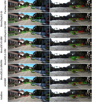
Figure 4: 3D object detection for different MDE methods combined with Point R-CNN. Red BBs are ground truth, green ones are detections.

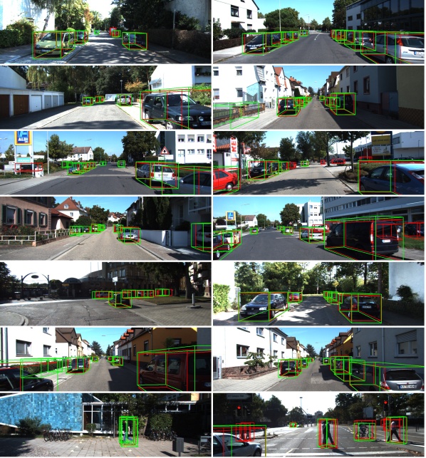
Figure 5: 3D object detection based on MonoDELSNet-St combined with Point R-CNN.

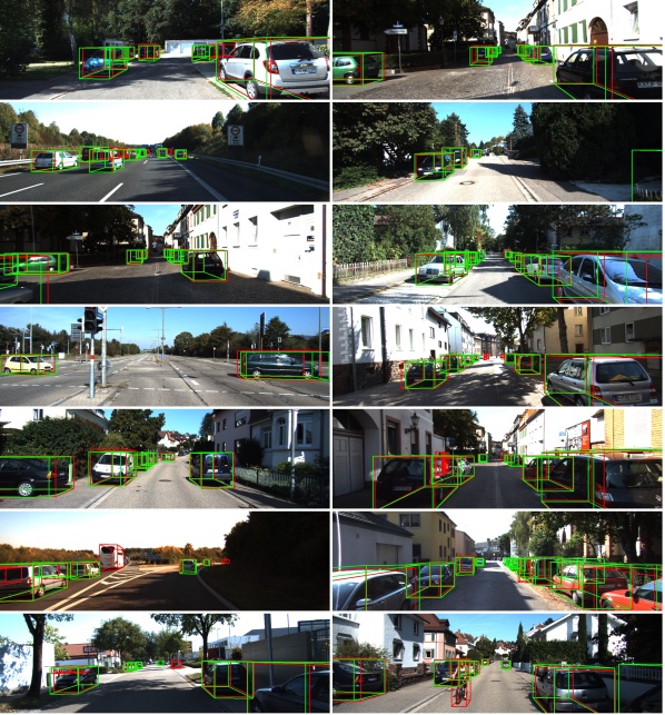
Figure 6: 3D object detection based on MonoDELSNet-St combined with Voxel R-CNN.

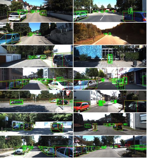
Figure 7: 3D object detection based on MonoDELSNet-St combined with CenterPoint.

4.4 Depth estimation vs. 3D object detection

Despite examining the results of Table 2 and Table 3 has a great interest in itself, in this paper, we focus on confronting them. Concerning the 3D object detection metrics, it is common practice to focus on the moderate setting (mod.). Moreover, we see in Table 2 that $AP_{BEV}$ and $AP_{3D}$ give rise to analogous rankings in terms of 3D object detection under the moderate setting. Thus, for the shake of simplicity, we are going to focus only on $AP_{BEV}$. Accordingly, Fig. 8 compares the $AP_{BEV}-mod$ ranking with the abs-rel, rms, and $\delta<\tau$ $(\tau=1.25)$ rankings, for all the considered 3D object detection models. Briefly, the correspondence between MDE and object detection rankings can be visually observed by looking at the arrows in these figures. A perfect correspondence between rankings shows as parallel arrows, while the lower the correspondence, the more arrows crossing each other. Taking this into account, it is clear that the MDE metric abs-rel predicts the 3D object detection results better than the others. The $\delta<\tau$ metric is more messy, and rms metric is performing in between the other two.

Figure 8: Comparing rankings: abs-rel, rms, $\delta<1.25$ (MDE) vs. $AP_{BEV}-mod$ (3D OD). In the mid column, we have ordered the MDE models from best (top/1) to worse (bottom/8). Then, we have replicated the mid columns as left (voxel-based detectors, which produce the same ranking) and right (Point R-CNN) columns. Afterwards, we have connected the models in left and right columns to its ranking number according to $AP_{BEV}-mod$. Thus, a perfect correspondence between rankings shows as parallel arrows, while the lower the correspondence, the more arrows crossing each other. We abbreviate MonoDepth2 as MD2, MonoDEVSNet as MDEVS, MonoDELSNet as MDELS.

5 Conclusion

When performing MDE on-board an autonomous or assisted vehicle, obtaining depth estimation maps is just an intermediate step of a perception stack. For instance, the perception goal may be to perform semantic segmentation or/and object detection with attached depth information to allow for actual vehicle navigation. On the other hand, reviewing the literature of MDE, it is common to see relatively small quantitative differences among the evaluated MDE models. Thus, one may wonder if those differences will be consolidated once such MDE models are used in the targeted perception task. We have addressed this question by using 3D object detection as target perception task. Depth maps based on different MDE models have been converted to Pseudo-LiDAR 3D point clouds, where 3D object detectors can be trained and tested. We have considered eight MDE models, as well as three different CNN architectures for 3D object detection (Point R-CNN, Voxel R-CNN, CenterPoint). Using KITTI benchmark data, we have seen that, indeed, the abs-rel metric commonly used in MDE assessment, is well aligned with 3D object detection results in terms of ranking the MDE methods. What remains as future work is to investigate if we can predict accuracy improvements in 3D object detection (in absolute terms), from the improvements observed in the abs-rel metric. In case this is not possible, we recommend to incorporate 3D object detection as part of the evaluation of MDE models. It is worth to mention that we have also seen that the way depth maps are sampled to produce Pseudo-LiDAR matters because of the dependency that 3D object detectors have on this.

References

- [1] Shariq Farooq Bhat, Ibraheem Alhashim, and Peter Wonka. Adabins: Depth estimation using adaptive bins. In Int. Conf. on Computer Vision and Pattern Recognition (CVPR), 2021.
- [2] Y. Cao, Z. Wu, and C. Shen. Estimating depth from monocular images as classification using deep fully convolutional residual networks. IEEE Trans. on Circuits and Systems for Video Technology, 2017.
- [3] Po-Yi Chen, Alexander H. Liu, Yen-Cheng Liu, and Yu-Chiang Frank Wang. Towards scene understanding: Unsupervised monocular depth estimation with semantic-aware representation. In Int. Conf. on Computer Vision and Pattern Recognition (CVPR), 2019.
- [4] Xiaozhi Chen, Kaustav Kundu, Yukun Zhu, Andrew G Berneshawi, Huimin Ma, Sanja Fidler, and Raquel Urtasun. 3d object proposals for accurate object class detection. In Neural Information Processing Systems (NeurIPS), 2015.
- [5] Raul de Queiroz Mendes, Eduardo Godinho Ribeiro, Nicolas dos Santos Rosa, and Valdir Grassi Jr. On deep learning techniques to boost monocular depth estimation for autonomous navigation. Robotics and Autonomous Systems, 136:103701, February 2021.
- [6] Jiajun Deng, Shaoshuai Shi, Peiwei Li, Wengang Zhou, Yanyong Zhang, and Houqiang Li. Voxel R-CNN: Towards high performance voxel-based 3d object detection. In Proceedings of the AAAI Conference on Artificial Intelligence, 2021.
- [7] D. Eigen, C. Puhrsch, and R. Fergus. Depth map prediction from a single image using a multi-scale deep network. In Neural Information Processing Systems (NeurIPS), 2014.
- [8] R. Garg, V. Kumar, G. Carneiro, and I. Reid. Unsupervised cnn for single view depth estimation: Geometry to the rescue. In European Conference on Computer Vision (ECCV), 2016.
- [9] A. Geiger, P. Lenz, C. Stiller, and R. Urtasun. Vision meets robotics: The KITTI dataset. International Journal of Robotics Research, 32(11):1231–1237, 2013.
- [10] C. Godard, O.M. Aodha, and G.J. Brostow. Unsupervised monocular depth estimation with left-right consistency. In Int. Conf. on Computer Vision and Pattern Recognition (CVPR), 2017.
- [11] Clément Godard, Oisin Mac Aodha, Michael Firman, and Gabriel J. Brostow. Digging into self-supervised monocular depth estimation. In International Conference on Computer Vision (ICCV), 2019.
- [12] Vitor Guizilini, Rares Ambrus, Sudeep Pillai, Allan Raventos, and Adrien Gaidon. 3D packing for self-supervised monocular depth estimation. In Int. Conf. on Computer Vision and Pattern Recognition (CVPR), 2020.
- [13] Akhil Gurram, Ahmet Faruk Tuna, Fengyi Shen, Onay Urfalioglu, and Antonio M. López. Monocular depth estimation through virtual-world supervision and real-world sfm self-supervision. IEEE Transactions on Intelligent Transportation Systems, pages 1–14, 2021.
- [14] Akhil Gurram, Ahmet Faruk Tuna, Fengyi Shen, Onay Urfalioglu, and Antonio M. López. Monocular depth estimation through virtual-world supervision and real-world SfM self-supervision, 2022.
- [15] Akhil Gurram, Onay Urfalioglu, Ibrahim Halfaoui, Fahd Bouzaraa, and Antonio M. López. Monocular depth estimation by learning from heterogeneous datasets. In Intelligent Vehicles Symposium (IV), 2018.
- [16] Y. Kuznietsov, J. Stückler, and B. Leibe. Semi-supervised deep learning for monocular depth map prediction. In Int. Conf. on Computer Vision and Pattern Recognition (CVPR), 2017.
- [17] Alex H Lang, Sourabh Vora, Holger Caesar, Lubing Zhou, Jiong Yang, and Oscar Beijbom. Pointpillars: Fast encoders for object detection from point clouds. In Int. Conf. on Computer Vision and Pattern Recognition (CVPR), 2019.
- [18] Buyu Li, Wanli Ouyang, Lu Sheng, Xingyu Zeng, and Xiaogang Wang. Gs3d: An efficient 3d object detection framework for autonomous driving. In Int. Conf. on Computer Vision and Pattern Recognition (CVPR), 2019.
- [19] F. Liu, C. Shen, G. Lin, and I. Reid. Learning depth from single monocular images using deep convolutional neural fields. IEEE Trans. on Pattern Analysis and Machine Intelligence, 38(10):2024–2039, 2016.
- [20] Wei Liu, Dragomir Anguelov, Dumitru Erhan, Christian Szegedy, Scott Reed, Cheng-Yang Fu, and Alexander C Berg. Ssd: Single shot multibox detector. In European Conference on Computer Vision (ECCV), 2016.
- [21] Li Long and Shan Dongri. Review of camera calibration algorithms. In Sanjiv K. Bhatia, Shailesh Tiwari, Krishn K. Mishra, and Munesh C. Trivedi, editors, Advances in Computer Communication and Computational Sciences, pages 723–732. Springer Singapore, 2019.
- [22] Jogendra Nath Kundu, Phani Krishna Uppala, Anuj Pahuja, and R. Venkatesh Babu. AdaDepth: Unsupervised content congruent adaptation for depth estimation. In Int. Conf. on Computer Vision and Pattern Recognition (CVPR), 2018.
- [23] Koutilya PNVR, Hao Zhou, and David Jacobs. SharinGAN: Combining synthetic and real data for unsupervised geometry estimation. In Int. Conf. on Computer Vision and Pattern Recognition (CVPR), 2020.
- [24] Charles R Qi, Hao Su, Kaichun Mo, and Leonidas J Guibas. Pointnet: Deep learning on point sets for 3d classification and segmentation. In Int. Conf. on Computer Vision and Pattern Recognition (CVPR), 2017.
- [25] Charles Ruizhongtai Qi, Li Yi, Hao Su, and Leonidas J Guibas. Pointnet++: Deep hierarchical feature learning on point sets in a metric space. Advances in Neural Information Processing Systems, 30:5099–5108, 2017.
- [26] S. Ren, K. He, R. Girshick, and J. Sun. Faster R-CNN: Towards real time object detection with region proposal networks. IEEE Trans. on Pattern Analysis and Machine Intelligence, 39(6):1137–1149, 2017.
- [27] Shaoshuai Shi, Xiaogang Wang, and Hongsheng Li. PointRCNN: 3D object proposal generation and detection from point cloud. In Int. Conf. on Computer Vision and Pattern Recognition (CVPR), 2019.
- [28] Yan Wang, Wei-Lun Chao, Divyansh Garg, Bharath Hariharan, Mark Campbell, and Kilian Q Weinberger. Pseudo-LiDAR from visual depth estimation: Bridging the gap in 3D object detection for autonomous driving. In Int. Conf. on Computer Vision and Pattern Recognition (CVPR), 2019.
- [29] Dan Xu, Wei Wang, Hao Tang, Hong Liu, Nicu Sebe, and Elisa Ricci. Structured attention guided convolutional neural fields for monocular depth estimation. In Int. Conf. on Computer Vision and Pattern Recognition (CVPR), 2018.
- [30] Zetong Yang, Yanan Sun, Shu Liu, and Jiaya Jia. 3DSSD: Point-based 3d single stage object detector. In Int. Conf. on Computer Vision and Pattern Recognition (CVPR), 2020.
- [31] Tianwei Yin, Xingyi Zhou, and Philipp Krahenbuhl. Center-based 3D object detection and tracking. In Int. Conf. on Computer Vision and Pattern Recognition (CVPR), 2021.
- [32] Zhichao Yin and Jianping Shi. GeoNet: Unsupervised learning of dense depth, optical flow and camera pose. In Int. Conf. on Computer Vision and Pattern Recognition (CVPR), 2018.
- [33] Yurong You, Yan Wang, Wei-Lun Chao, Divyansh Garg, Geoff Pleiss, Bharath Hariharan, Mark Campbell, and Kilian Q Weinberger. Pseudo-lidar++: Accurate depth for 3d object detection in autonomous driving. In International Conference on Learning Representation (ICLR), 2019.
- [34] Shanshan Zhao, Huan Fu, Mingming Gong, and Dacheng Tao. Geometry-aware symmetric domain adaptation for monocular depth estimation. In Int. Conf. on Computer Vision and Pattern Recognition (CVPR), 2019.
- [35] Wang Zhao, Shaohui Liu, Yezhi Shu, and Yong-Jin Liu. Towards better generalization: Joint depth-pose learning without PoseNet. In Int. Conf. on Computer Vision and Pattern Recognition (CVPR), 2020.
- [36] Chuanxia Zheng, Tat-Jen Cham, and Jianfei Cai. T2Net: Synthetic-to-realistic translation for solving single-image depth estimation tasks. In European Conference on Computer Vision (ECCV), 2018.
- [37] T. Zhou, M. Brown, N. Snavely, and D. Lowe. Unsupervised learning of depth and ego-motion from video. In Int. Conf. on Computer Vision and Pattern Recognition (CVPR), 2017.
- [38] Xingyi Zhou, Dequan Wang, and Philipp Krähenbühl. Objects as points. arXiv preprint arXiv:1904.07850, 2019.
- [39] Yin Zhou and Oncel Tuzel. VoxelNet: End-to-end learning for point cloud based 3D object detection. In Int. Conf. on Computer Vision and Pattern Recognition (CVPR), 2018.