Optimizing the magnon-phonon cooperativity in planar geometries
Abstract
Optimizing the cooperativity between two distinct particles is an important feature of quantum information processing. Of particular interest is the coupling between spin and phonon, which allows for integrated long range communication between gates operating at GHz frequency. Using local light scattering, we show that, in magnetic planar geometries, this attribute can be tuned by adjusting the orientation and strength of an external magnetic field. The coupling strength is enhanced by about a factor of 2 for the out-of-plane magnetized geometry where the Kittel mode is coupled to circularly polarized phonons, compared to the in-plane one where it couples to linearly polarized phonons. We also show that the overlap between magnon and phonon is maximized by matching the Kittel frequency with an acoustic resonance that satisfies the half-wave plate condition across the magnetic film thickness. Taking the frequency dependence of the damping into account, a maximum cooperativity of about 6 is reached in garnets for the normal configuration near 5.5 GHz.
Quantum information processing relies on the coherent interconversion process between distinct particles. Among the candidates, the coupling between magnons and phonons offers a certain advantage in terms of tunability and long-range propagation distance, which make them useful for building an efficient quantum transducer Lachance-Quirion et al. (2019). Magnetically driven circularly polarized phonons can also carry angular momentum Zhang and Niu (2014); Garanin and Chudnovsky (2015) and transfer it over a characteristic distance much longer than that of magnons without requiring a magnetic material An et al. (2020); Schlitz et al. (2022); Rückriegel and Duine (2020). This new direction in spintronics has created a surge of interest in using phonon angular momentum to enable long-distance spin transport Brataas et al. (2020); Li et al. (2021). Furthermore, phonons are tunable via the geometry and size, raising the hope of optimizing the conversion process Mondal et al. (2018); Berk et al. (2019); Godejohann et al. (2020).
The mutual coupling can be interpreted as an interaction between lattice displacement and magnetic orientation via magnetostriction Kittel (1958); Spencer and LeCraw (1958); Schlömann (1960); Matthews and LeCraw (1962); Lee (1955) or microscopically in terms of magnon-phonon interaction Guerreiro and Rezende (2015); Holanda et al. (2018); Rezende et al. (2021). The coupling results in the formation of magnon-polaron hybrid states Shen and Bauer (2015) that are split by the coupling strength, . Experimentally strong coupling has been demonstrated in various systems such as magnetic insulators Zhang et al. (2016); Khivintsev et al. (2018), metals Zhao et al. (2020), semiconductors Kuszewski et al. (2018), and nano-fabricated ferromagnets Berk et al. (2019); Godejohann et al. (2020).
To gain control over the interconversion process, one needs to develop a way to tune the cooperativity Turchette et al. (1998); Tuchman et al. (2006); Kuhn and Ljunggren (2010); Reiserer and Rempe (2015); Al-Sumaidae et al. (2018); Thomas et al. (2022), a figure of merit which measures the number of oscillations that occurs between the two waveforms before decoherence starts to kick in. Here and are the relaxation rates of magnons and phonons, respectively. The relaxation rates are related to the material quality issue and are challenging to control, but tuning the coupling strength can provide a more efficient way to control due to its dependence. The manipulation of coupling strength between magnons and microwave photons has been achieved by changing the position of magnetic system Harder et al. (2018); Xu et al. (2019); Ihn et al. (2020). But this scheme is hard to apply for the magnon-phonon coupled system because two bodies are inseparable.
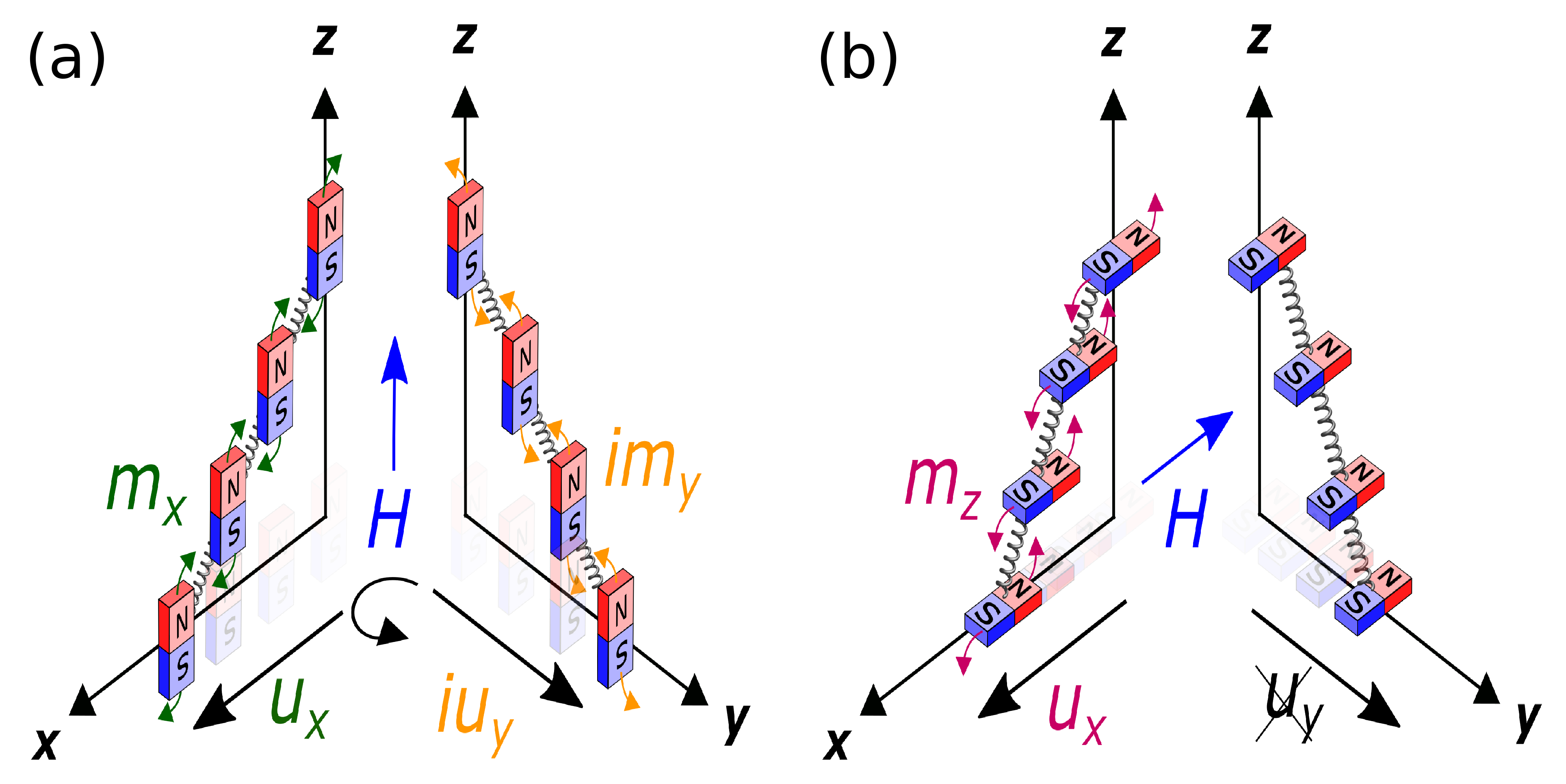
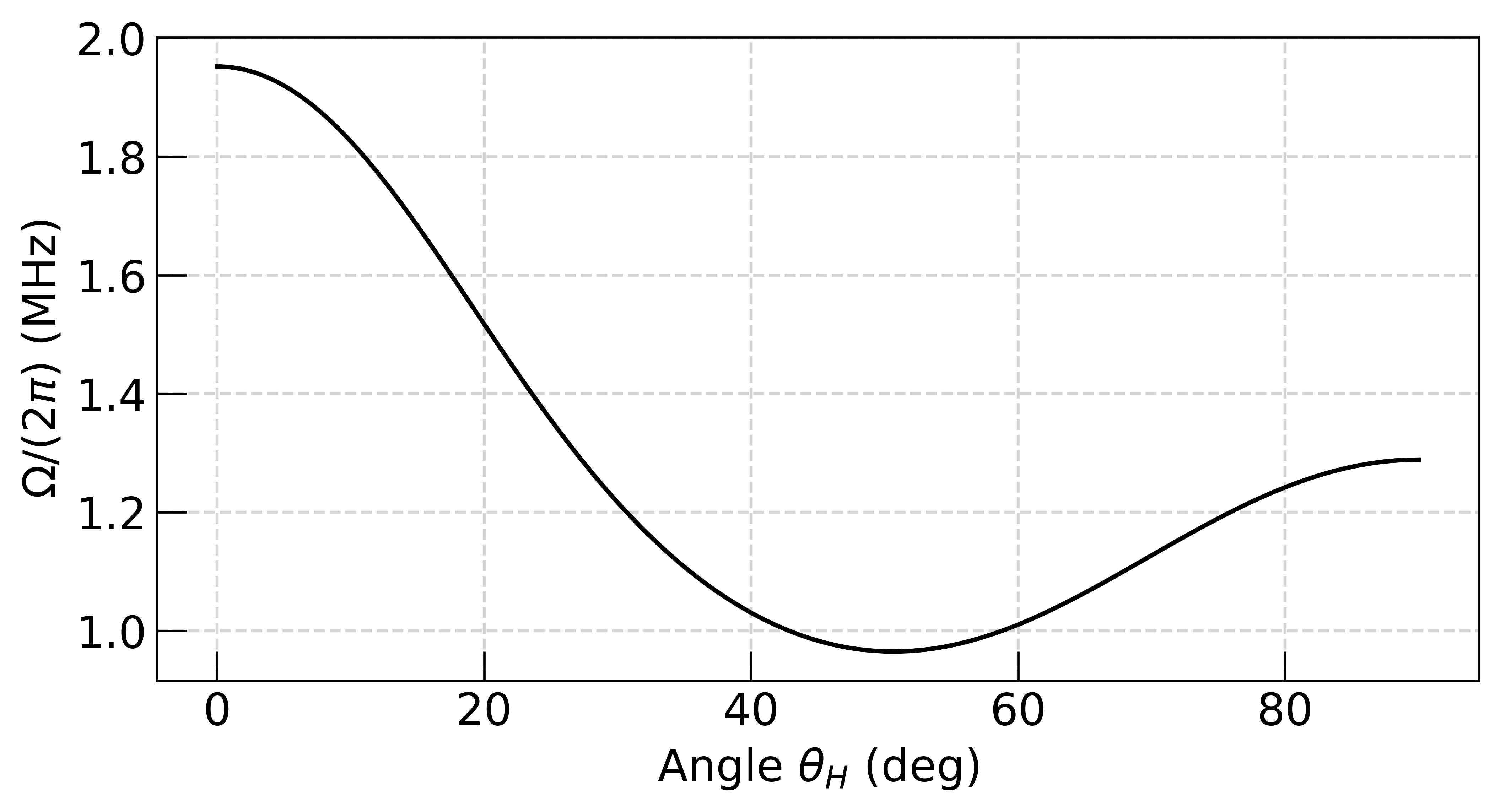
For magnon-phonon coupled systems, the coupling stength can be tuned by adjusting the magnetoelastic energy Morgenthaler (1963); Comstock and LeCraw (1963). For the normally magnetized case, the strains from both transverse lattice vibrations, and , give rise to the change in magnetization alignment (Fig. 1(a)). This contributes to the magnetoelastic energy ), where , , and represent the static, dynamical parts of the magnetization, and the lattice vibration along the direction, respectively. is the direction normal to the film surface. An analytic form of the coupling strength for this configuration is presented in Appendix A. For the in-plane magnetized case, however, only the lattice displacement along the direction of magnetic field ( in Fig. 1(b)) couples to the magnetoelastic energy, leading to . This difference in results in about 1.7 times weaker coupling strength for the in-plane magnetized case at (see Appendix B). Other than these two field directions, an analytic expression for the coupling strength has a complex form and a full angular dependence of coupling strength is presented in Appendix C.
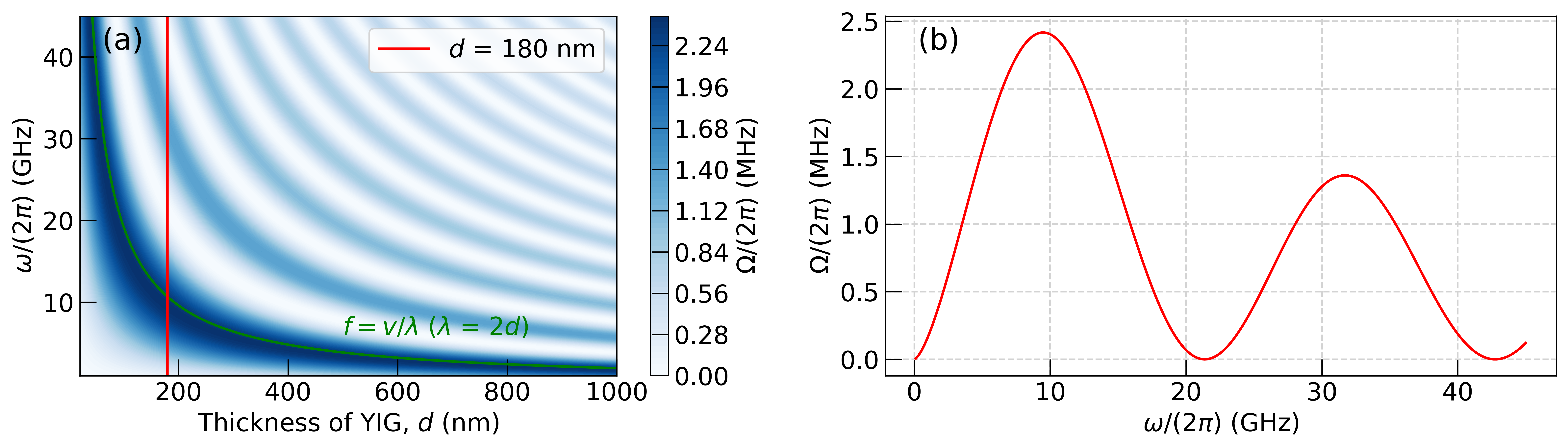
The increased coupling strength for circularly polarized phonons (as in the case of out-of-plane field) is due to the simultaneous contribution of both orthogonal lattice vibrations, leading to a larger magneto-elastic energy. For the linearly polarized phonons (as in the case of in-plane magnetized case), only the component of the lattice vibration parallel to the field direction couples to the magnetization dynamics, hence leading to less effective coupling. This discrepancy accounts for an approximate two-fold enhancement in the coupling strength of circularly polarized phonons. However this enhancement factor may differ depending on the nature of phonon modes and their propagation directions relative to crystallographic axes. Furthermore, the coupling strength in thin magnetic films also depends on the overlap between the magnon and phonon wave functions Litvinenko et al. (2021); Schlitz et al. (2022). This can be tuned by changing the phonon wavelength over the thin magnetic layer. For the uniform Kittel mode, the maximum coupling is achieved when the phonon half wavelength is equal to the thickness of the magnetic layer. On the other hand, the maximum coupling between spatially nonuniform magnon modes and phonons satisfies a different condition Schlitz et al. (2022).
In our experiments, the magnon phonon coupling is detected optically by micro-Brillouin light scattering (BLS), which has the advantage of sensing magnons or phonons directly over the laser spot size of a few microns. The local detection also reduces the contributions from spatial inhomogeneities, minimizing spectral broadening, which allows sensitive detection of coupling between quasiparticles Bozhko et al. (2017); Holanda et al. (2018); Frey et al. (2021). Typical BLS experiments, however, have a limited spectral resolution on the order of ten MHz Demokritov and Demidov (2007); Sebastian et al. (2015), which is not enough to resolve of a few MHz range.
Here we show that the microwave excited BLS can overcome this limit and sense magnon-polarons with enhanced contrast at the avoided crossing. This improvement comes from reducing the adverse effects of spatial inhomogeneities. We perform experiments with both in-plane and out-of-plane magnetic field configurations. Stronger magnon-phonon coupling is observed upon applying the magnetic field to the out-of-plane direction, consistent with the illustration in Fig. 1. We show that the coupling strength is further tunable via changing the phonon wavelength.
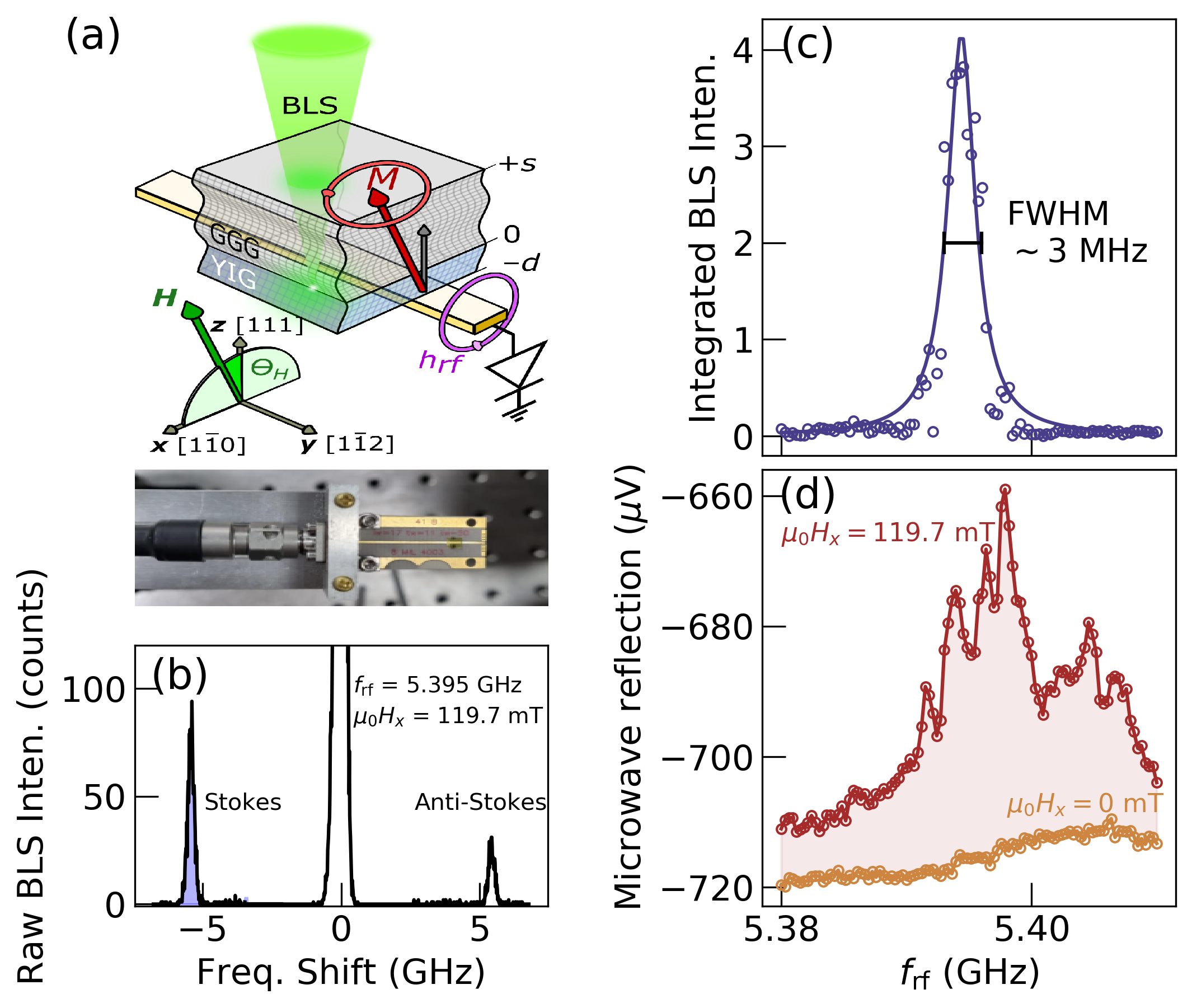
We use a thick yttrium iron garnet (YIG) grown on a m thick gadolinium gallium garnet (GGG) by the liquid phase epitaxy method, followed by removing one side of the originally double-sided YIG via ion-beam etching. The lateral size of 2 mm 2 mm sample is placed on top of a m wide strip antenna (see Fig. 2(a)). An amplitude-modulated microwave at a frequency of 3177 Hz is applied to the sample through a circulator to measure the microwave absorption spectrum. The reflected power is sent to a diode detector and is recorded using a lock-in amplifier. Simultaneously a 37 mW green laser is focused to a beam diameter of 4 m at the bottom of the sample, where the YIG layer is placed, via a 20 objective lens. The beam position is fixed at about 50 m away from the edge of antenna. The laser has a penetration depth of 6 m in YIG Scott et al. (1974), and it is transparent to GGG. As a result, it can penetrate the entire sample without any significant absorption. The component of the antenna field, , is at its maximum near the edge of the antenna, where it exerts the maximum torque on magnetization with the in-plane bias field An et al. (2014). A cross-polarized back-scattered light is sent to a tandem Fabry-Perot interferometer, where the frequency shift of scattered light is analyzed. The external magnetic field can be applied along the in-plane or out-of-plane directions. A pair of secondary Helmholtz coils is used to control the magnetic field on the order of tens of T.
The raw BLS spectrum under microwave excitation is shown in Fig. 2(b). Thermally excited magnon signals in our thin film YIG lie under the noise level. The microwave-assisted magnon signals are more substantial and typically show about 100 counts/s at the peak with an excitation power of dBm. The two peak positions labeled by Stokes and Anti-Stokes peaks in the raw spectrum are identical to the excitation microwave frequency (). Here, the magnon linewidth is determined by the instrumental limit, which is about 300 MHz close to the linewidth of the peak located at zero frequency shift. The Stokes peak area is then integrated, and the integrated intensity is plotted as a function of in Fig. 2(c), where a lorentzian function fits the data. Here the full linewidth is about 3 MHz, comparable to the previously reported values LeCraw et al. (1958); Beaulieu et al. (2018). The wavevector of magnons dominantly contributing to the spectrum is as the antenna coupling is less efficient for values larger than , where is the antenna width Kalinikos (1980). In our backscattering geometry, the bulk standing wave phonons are not detected due to wavevector mismatch 111The bulk phonon wave vector that satisfies the momentum conservation for our backscattering geometry is given by , where and are the scattered and incident light wave vectors. The refractive index is about 2 for GGG. With for the transverse sound wave, the phonon signal is expected and detected at about 26 GHz. The simultaneously obtained microwave reflection spectrum is shown in Fig. 2(d). The two spectra taken at 119.7 mT and 0 mT are compared, where the latter represents the background antenna reflection. The difference (red shaded area in Fig. 2(d)) shows the absorbed microwave power by the magnetic system. A broad resonance spectrum composed of multiple sharp peaks is obtained. The spectral broadening is attributed to the spatially inhomogeneous magnetic precession over the large detection area covered by the antenna.
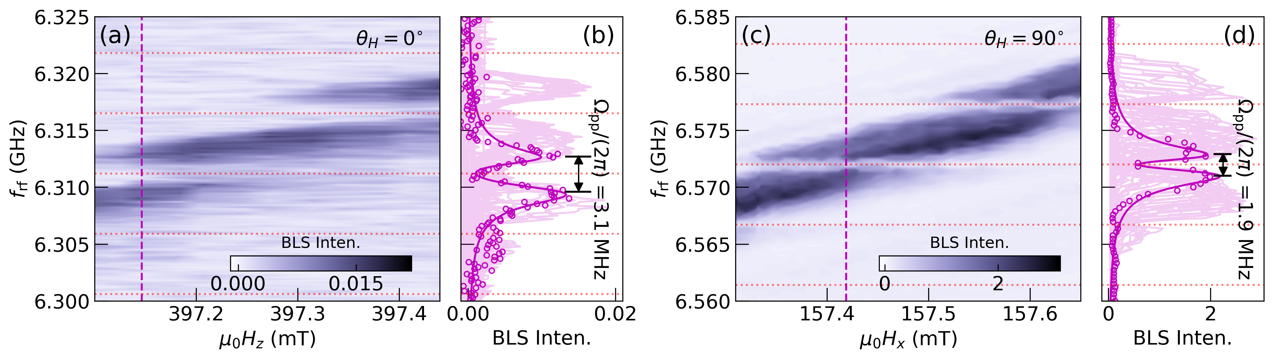
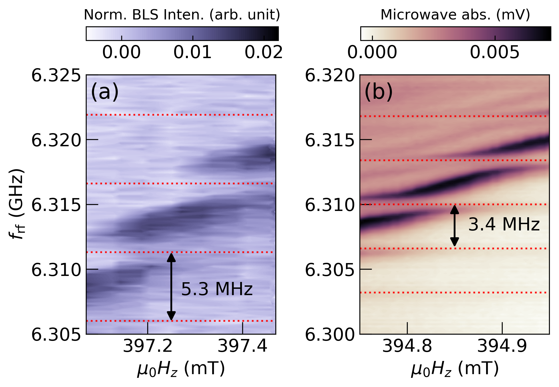
With the capability of locally probing the dynamic magnetization, we now demonstrate the excellent sensitivity of BLS to the formation of magnon-polarons for out-of-plane magnetized configuration by applying . Here the signal-to-noise ratio in the BLS measurement is low because BLS is less sensitive to the in-plane dynamic magnetization Hamrle et al. (2010). To compensate for this, the BLS spectrum is taken at the middle of the antenna to maximize the torque by . Figure 3(a) shows the integrated BLS intensity as a function of and excitation frequency. We clearly see strongly reduced intensities of down to 90% at each phonon frequency indicated by the red dotted lines. These are regularly placed at , where is an integer, is the transverse phonon velocity in GGG, and are the YIG and GGG thickness values, respectively. With Ye and Dötsch (1991), we obtain a frequency spacing of , close to the measured frequency spacing of 5.24 MHz. This spacing is enlarged compared to the previous works that used thicker GGG substrates (see Appendix E). The phonon-induced gap is about , where is slightly larger than the actual coupling strength by . With and extracted from the fit shown as the purple solid line in Fig. 3(b), we obtain .
Based on the picture illustrated in Fig. 1, we expect a reduced magnon-phonon coupling for the in-plane magnetized configuration, where lattice vibrations become linear. Figure 3(c) shows the spectra obtained upon applying the in-plane magnetic field at a similar frequency range to that of Fig. 3(a). The phonon-induced gap of is reduced to (Fig. 3(c)). With and , we obtain . This shows that there is a factor of 2 enhancement in for the out-of-plane magnetized case. In terms of , this represents a factor of 4 improvement. In addition, there is no sign of coupling between longitudinal phonons and magnons, which would give a larger frequency spacing 222Longitudinal phonons have Kleszczewski and Bodzenta (1988), which would lead to 9.7 MHz frequency spacing, not visible in Fig. 3(c)., an experimental evidence that the phonons are indeed transverse-linearly polarized for the in-plane magnetized case Streib et al. (2018). Additionally, it is worth noting that similar acoustic damping values of were obtained for both the out-of-plane and in-plane field cases. This suggests a close proximity in the damping rates between circularly polarized and linearly polarized phonons.
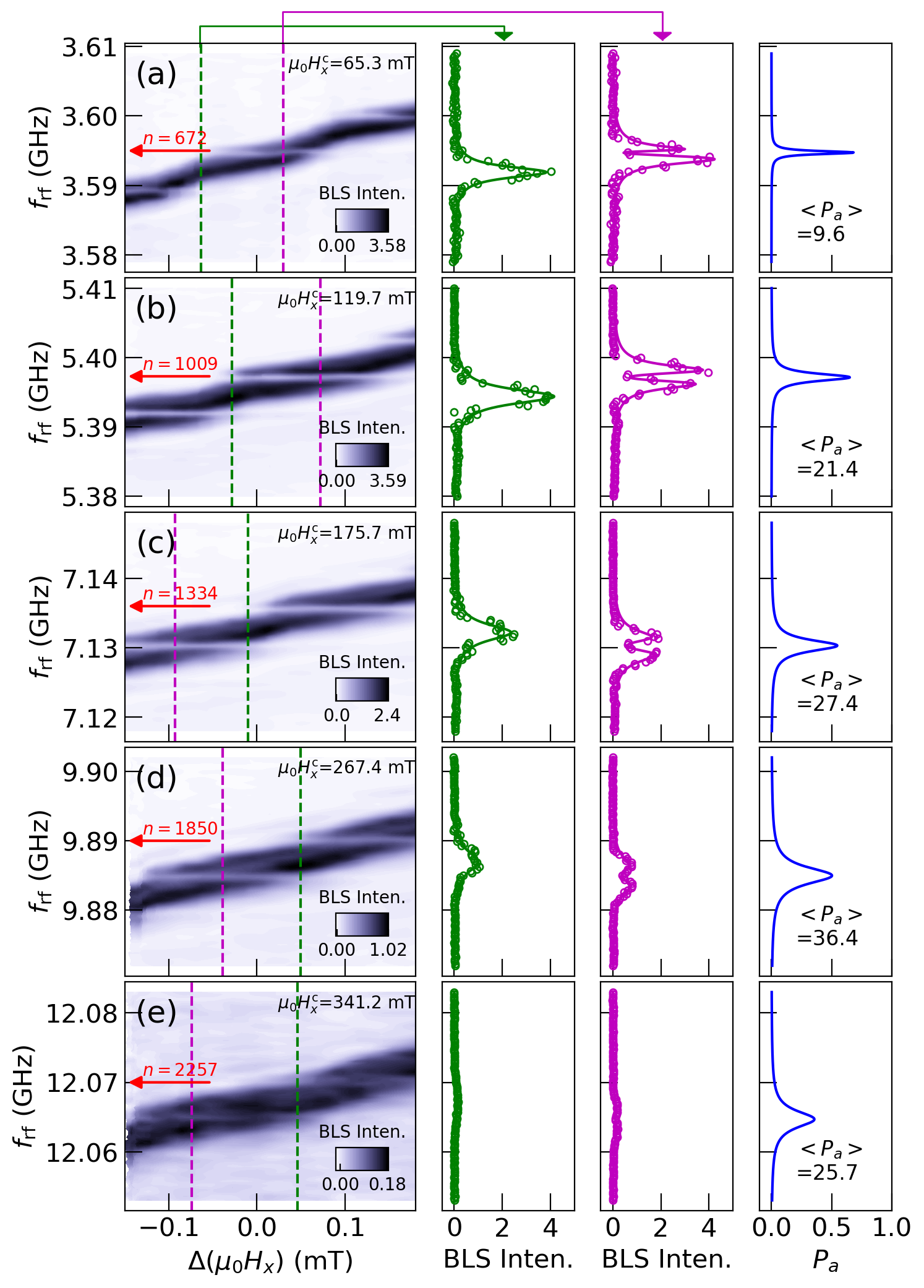
Next, we discuss experiments with different phonon wavelengths by changing the central field, for an in-plane magnetized case. Figure 4(a-e) shows the field and frequency-dependent BLS spectra at different central phonon mode indices indicated by the red arrows. The integrated BLS intensities are plotted in the first column of Fig. 4, where the color scales are normalized to the maxima. The magnon resonances broaden, and the phonon dips reduce with increasing . The absolute BLS intensity significantly drops for higher (see the second and third columns of Fig. 4) due to increased magnon damping, which is proportional to 333We also observed an increased microwave insertion loss of about 3 dBm over the studied frequency range, which may account for an additional reduction of signal at high frequencies. The green linecut is drawn over where the magnon phonon coupling is not visible, therefore pure magnetic resonances are obtained. The purple line cut is drawn to characterize the magnon-polarons.
To perform quantitative analysis, we use the two coupled oscillator model described as follows An et al. (2020):
| (1) |
where are circularly polarized magnon/phonon amplitudes and are the magnetic/acoustic relaxation rates. are the magnetic/acoustic resonances, is the coupling to the antenna, is the antenna field. By solving Eq. 1, we obtain analytic expressions for and given by
| (2) |
The measured BLS intensity is proportional to Buchmeier et al. (2007); Birt et al. (2012) that we use to fit the experimental data. The green lines in Fig. 4 correspond to the fit without phonon contributions, i.e., and from which we extract and . Then, we fit the case with magnon polarons (purple lines in Fig. 4) to extract , and . With these parameters, the complementary can be calculated based on Eq. 2. We then estimate the relative power transferred to the phonon system by
| (3) |
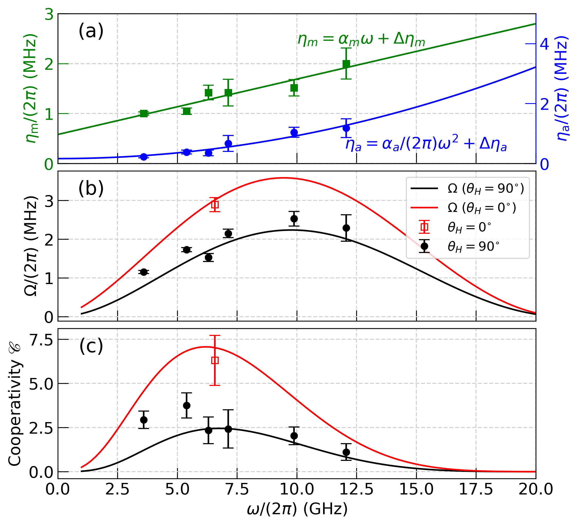
At low , becomes larger than 50% (see the fourth column of Fig. 4). The spectral integration, , becomes maximum near 9 GHz, where the magnon phonon coupling reaches the maximum (see Fig. 5(b)). It is important to note that the experimentally obtained spectral shape consistently aligns with , confirming that our BLS method detects the magnon signal instead of phonons.
The frequency dependences of , , , and are summarized in Fig. 5. follows the predicted linear frequency dependence well (green solid line in Fig. 5(a)) from which we extract , which is close to literature value Dubs et al. (2017), and the inhomogeneous line broadening of . A quadratic dependence on frequency is expected for acoustic damping (blue solid line in Fig. 5(a)) Dutoit (1974). We extract an acoustic relaxation rate of and an inhomogeneous contribution of , which are in reasonable agreements with previously reported values Kleszczewski and Bodzenta (1988); Schlitz et al. (2022). The coupling strength for the in-plane magnetized case is given by (see Appendix B for derivation)
| (4) |
where , is the density of YIG, and is the saturation magnetization. represents the effective magnetoelastic coefficient. We use , , , and the known transverse sound velocity Clark and Strakna (1961). The expected coupling strength variation for in-plane (Eq. 4) and out-of-plane (Eq. A5) magnetized cases are shown with as solid lines in Fig. 5(b). We note that it works well for both in-plane and out-of-plane configurations. However this estimate of deviates from the theoretical value obtained with the known material parameters and assumed pinning free boundary conditions, (see Appendix B). We attribute the discrepancy to the several assumptions made in the calculations, i.e., unpinned spins at the boundaries, phonon properties assumed to be identical for the YIG film and GGG substrates, and neglected anisotropy fields Polulyakh et al. (2021). This calls for detailed investigation on magnetoelastic properties in thin films. Additionally, it is important to note that while our study primarily focuses on the excitation of magnons with , there is a possibility that high- magnons could also interact with phonons. This raises intriguing questions about the variations in cooperativity for high- magnons. Finally the frequency variation of cooperativity is shown Fig. 5(c). The maximum is achieved at lower frequency of about 5.5 GHz compared to 9 GHz for the optimal coupling strength due to the reduction of and with decreasing frequency.
In conclusion, the local magnon-phonon coupling was investigated using an optical technique. Enhanced contrast was observed at the phonon resonances due to the reduced nonuniformity over the detection area. Furthermore, we demonstrated tunable magnon phonon coupling and determined optimal parameters for maximizng magnon phonon interconversion in a planar geometry. Stronger coupling strength with the out-of-plane magnetized configuration was observed, which agrees with the calculations. Our local sensing scheme and optimization of the interconversion may find application to the coherent quantum information processing.
Acknowledgments
We thank Simon Streib for helpful discussions. This work was partially supported by the French Grants ANR-21-CE24-0031 Harmony and the EU-project H2020-2020-FETOPEN k-NET-899646; the EU-project HORIZON-EIC-2021-PATHFINDEROPEN PALANTIRI-101046630. K.A. acknowledges support from the National Research Foundation of Korea (NRF) grant (NRF-2021R1C1C2012269) funded by the Korean government (MSIT).
Appendix A : Magnetoelastic coupling strength in a thin magnetic film for the out-of-plane configuration
We derive an analytic form of coupling strength for out-of-plane magnetized case. We write the magnetic/acoustic equation of motion without damping and crystalline anisotropy terms Comstock and LeCraw (1963) :
| (A1) |
where and represent circularly polarized magnons and phonons. here represents the effective magnetoelastic coefficient when the out-of-plane field is applied along the [111] direction and is elastic stiffness constant. We assume that M and H are parallel.
With , , and , Eq. A1 can be written as
| (A2) |
where we approximated the phonon part with near the crossing point . We consider the coordinate system shown in Fig. 2(a). The magnon profile is for unpinned spins at the boundaries, where is the Heaviside step function. Phonon profile is , where is the index of the phonon mode. This assumes that the phonon amplitude becomes maximum at the boundaries. Coupling strength represents the anticrossing gap, . By integrating over the whole volume, we obtain
| (A3) |
The two equations are multiplied to yield
| (A4) |
where we applied the spatial integration. The integral on the right side can be evaluated using the properties of Heaviside step function and delta function, i.e., and . Finally, we obtain
| (A5) |
Appendix B : Magnetoelastic coupling in a thin magnetic film for the in-plane field configuration
The equation of motion needs to be modified when field is applied along the in-plane direction to take account of the change in (see Appendix F). In this case, the modified equation of motion is given as Polzikova et al. (2014)
| (B1) |
where is the magnetoelastic constants defined in Appendix F. The second equation for can be plugged in to yield
| (B2) |
where and Near the crossing point, we have and the above can be approximated as
| (B3) |
We perform the integration outlined in appendix A.
| (B4) |
Multiplying the two yields
| (B5) |
The imaginary term concerns the size of gap, which is much smaller than the resonance frequency. Ignoring this, we obtain
| (B6) |
Finally the coupling strength is given by
| (B7) |
where
| (B8) |
In our case, , , , and . Then , which amounts to 12% increase from .
The enhancement ratio is given by
| (B9) |
With , we obtain the ratio of about 1.5. This value is smaller than the experimental result of 1.9. To further improve the agreement, one needs to take into account more accurate pinning conditions and anisotropy fields.
Appendix C : Magnetoelastic coupling in a thin magnetic film for arbitrary magnetic field directions
The coupling strength between propagating phonons and spin waves for arbitrary field directions has been derived by E. Schlmann Schlömann (1960), which reads
| (C1) |
where represents the phonon wave vector and is the angle between the external magnetic field and the axis within the plane. For simplicity, we assume that the directions of magnetization and external magnetic field are always parallel, which is indeed the case for sufficiently large external field. is defined as
| (C2) |
Appendix D : Comparison between the BLS and FMR spectra
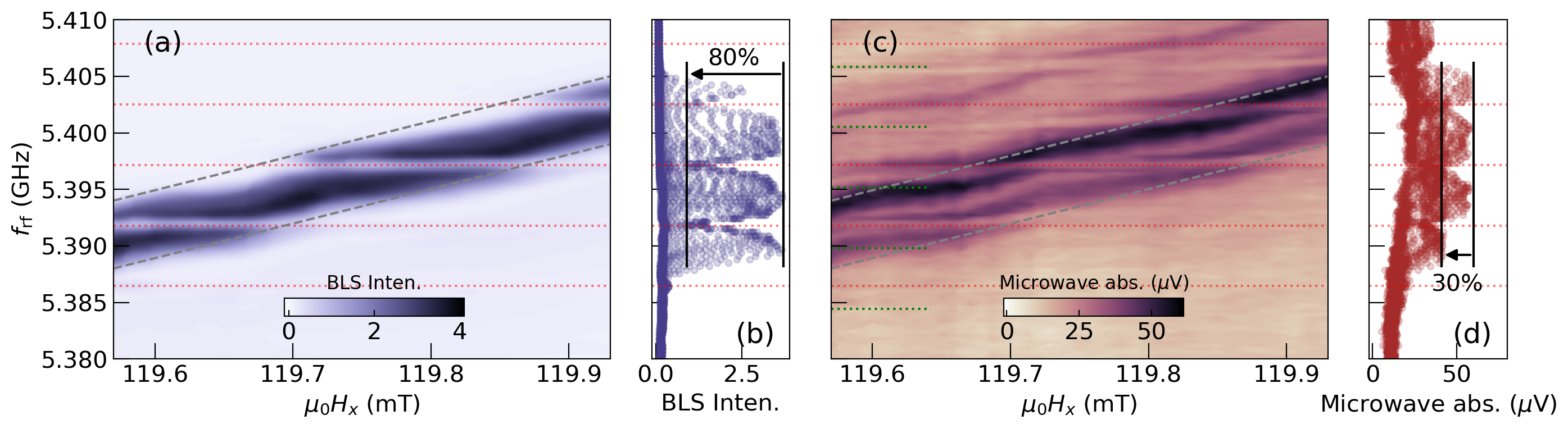
Here we provide a density plot of Fig. 2(d) as a function of field. In BLS, phonons are visible with a better contrast due to its local detection. The intensity reduces by 80% in Fig. 8(b) compared to the 30% reduction in Fig. 8(d) at the phonon resonances. The sharper contrast in BLS is attributed to the reduced detection area leading to a more homogeneous condition. Also multiple magnon lines are visible in the FMR spectrum as shown in Fig. 8(c). In addition to the main phonon lines indicated by red dotted lines, there is also a set of phonon lines visible indicated by green dotted lines.
Appendix E : Frequency spacing for different thicknesses of GGG substrates
The thickness of GGG determines the phonon frequencies following , where and are the YIG and GGG thickness. With the , we obtain and for 330 m and 500 m thick GGG substrates, respectively. These estimations are close to the measured frequency spacing shown in Fig. 9.
Appendix F : Magnetoelastic coefficients for the [10] direction
The value of changes depending on the direction of magnetization with the respect to the crystallographic axis. If the system is fully isotropic then we have . The difference between and would determines the variation of magnetoelastic energy with magnetization direction. The magnetoelastic energy then can be written as
| (F1) |
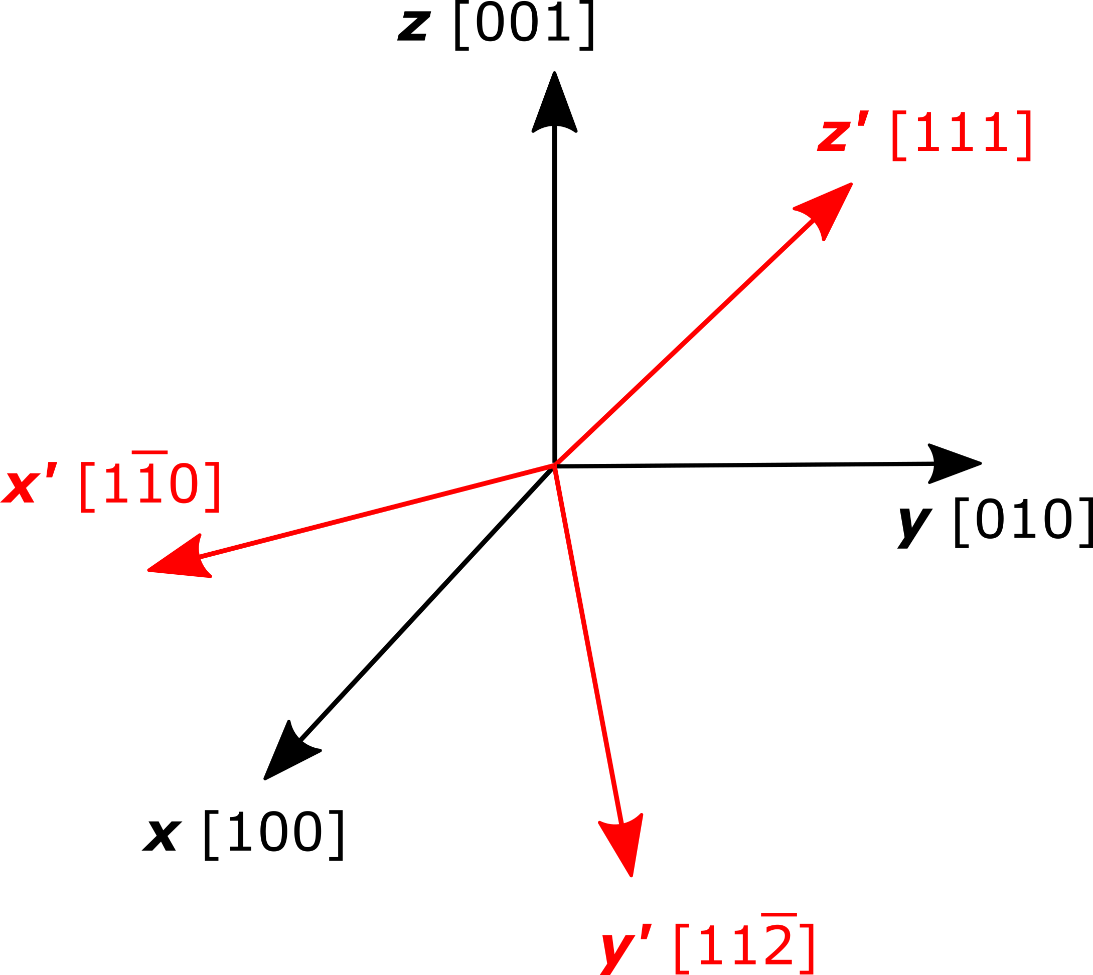
where and represents the strain tensor and the sum goes over . This form easily allows to extract when magnetized along the [001] direction. The coefficients of and terms are and , which represent the magnetoelastic constants for the longitudinal and transverse waves, respectively. When magnetized along the [111] direction, the transverse magnetoelastic coefficient is Comstock and LeCraw (1963). In our experiments, the in-plane field is applied along the [10] direction. To calculate the magnetoelastic energy in this case, one needs to perform a coordinate transform, where , , and (see Fig. 10). The transformation matrix is given by
| (F2) |
Since only the second part of Eq. F1 concerns the anisotropic nature of magnetoelastic coupling, the first part should be invariant under the coordinate transform. The transformation of the second part can be written as
| (F3) |
The magnetoelastic energy after this transformation has many terms. However most of them can be neglected in the first order approximation of dynamic magnetization. When the field is applied along the direction, and are the sole first order terms. Also we assume that the uniform magnetic precession excites the lattice. Therefore only and terms survive. The magnetoelastic energy therefore can be written as LeCraw and Comstock (1965)
| (F4) |
where , which is about three times smaller than . The modification due to the nonzero is considered for the calculation described in Appendix B.
References
- Lachance-Quirion et al. (2019) D. Lachance-Quirion, Y. Tabuchi, A. Gloppe, K. Usami, and Y. Nakamura, Hybrid quantum systems based on magnonics, Appl. Phys. Express 12, 070101 (2019).
- Zhang and Niu (2014) L. Zhang and Q. Niu, Angular momentum of phonons and the einstein–de haas effect, Phys. Rev. Lett. 112, 085503 (2014).
- Garanin and Chudnovsky (2015) D. Garanin and E. Chudnovsky, Angular momentum in spin-phonon processes, Phys. Rev. B 92, 024421 (2015).
- An et al. (2020) K. An, A. N. Litvinenko, R. Kohno, A. A. Fuad, V. V. Naletov, L. Vila, U. Ebels, G. de Loubens, H. Hurdequint, N. Beaulieu, et al., Coherent long-range transfer of angular momentum between magnon kittel modes by phonons, Phys. Rev. B 101, 060407 (2020).
- Schlitz et al. (2022) R. Schlitz, L. Siegl, T. Sato, W. Yu, G. E. Bauer, H. Huebl, and S. T. Goennenwein, Magnetization dynamics affected by phonon pumping, Phys. Rev. B 106, 014407 (2022).
- Rückriegel and Duine (2020) A. Rückriegel and R. A. Duine, Long-range phonon spin transport in ferromagnet–nonmagnetic insulator heterostructures, Phys. Rev. Lett. 124, 117201 (2020).
- Brataas et al. (2020) A. Brataas, B. van Wees, O. Klein, G. de Loubens, and M. Viret, Spin insulatronics, Phys. Rep. 885, 1 (2020).
- Li et al. (2021) Y. Li, C. Zhao, W. Zhang, A. Hoffmann, and V. Novosad, Advances in coherent coupling between magnons and acoustic phonons, APL Mater. 9, 060902 (2021).
- Mondal et al. (2018) S. Mondal, M. A. Abeed, K. Dutta, A. De, S. Sahoo, A. Barman, and S. Bandyopadhyay, Hybrid magnetodynamical modes in a single magnetostrictive nanomagnet on a piezoelectric substrate arising from magnetoelastic modulation of precessional dynamics, ACS Appl. Mater. Interfaces 10, 43970 (2018).
- Berk et al. (2019) C. Berk, M. Jaris, W. Yang, S. Dhuey, S. Cabrini, and H. Schmidt, Strongly coupled magnon–phonon dynamics in a single nanomagnet, Nat. Commun. 10, 1 (2019).
- Godejohann et al. (2020) F. Godejohann, A. V. Scherbakov, S. M. Kukhtaruk, A. N. Poddubny, D. D. Yaremkevich, M. Wang, A. Nadzeyka, D. R. Yakovlev, A. W. Rushforth, A. V. Akimov, et al., Magnon polaron formed by selectively coupled coherent magnon and phonon modes of a surface patterned ferromagnet, Phys. Rev. B 102, 144438 (2020).
- Kittel (1958) C. Kittel, Interaction of spin waves and ultrasonic waves in ferromagnetic crystals, Phys. Rev. 110, 836 (1958).
- Spencer and LeCraw (1958) E. G. Spencer and R. LeCraw, Magnetoacoustic resonance in yttrium iron garnet, Phys. Rev. Lett. 1, 241 (1958).
- Schlömann (1960) E. Schlömann, Generation of phonons in high-power ferromagnetic resonance experiments, J. Appl. Phys. 31, 1647 (1960).
- Matthews and LeCraw (1962) H. Matthews and R. LeCraw, Acoustic wave rotation by magnon-phonon interaction, Phys. Rev. Lett. 8, 397 (1962).
- Lee (1955) E. W. Lee, Magnetostriction and magnetomechanical effects, Rep. Prog. Phys. 18, 184 (1955).
- Guerreiro and Rezende (2015) S. C. Guerreiro and S. M. Rezende, Magnon-phonon interconversion in a dynamically reconfigurable magnetic material, Phys. Rev. B 92, 214437 (2015).
- Holanda et al. (2018) J. Holanda, D. Maior, A. Azevedo, and S. Rezende, Detecting the phonon spin in magnon–phonon conversion experiments, Nat. Phys. 14, 500 (2018).
- Rezende et al. (2021) S. Rezende, D. Maior, O. A. Santos, and J. Holanda, Theory for phonon pumping by magnonic spin currents, Phys. Rev. B 103, 144430 (2021).
- Shen and Bauer (2015) K. Shen and G. E. Bauer, Laser-induced spatiotemporal dynamics of magnetic films, Phys. Rev. Lett. 115, 197201 (2015).
- Zhang et al. (2016) X. Zhang, C.-L. Zou, L. Jiang, and H. X. Tang, Cavity magnomechanics, Sci. Adv. 2, e1501286 (2016).
- Khivintsev et al. (2018) Y. V. Khivintsev, V. Sakharov, S. Vysotskii, Y. A. Filimonov, A. Stognii, and S. Nikitov, Magnetoelastic waves in submicron yttrium–iron garnet films manufactured by means of ion-beam sputtering onto gadolinium–gallium garnet substrates, Tech. Phys. 63, 1029 (2018).
- Zhao et al. (2020) C. Zhao, Y. Li, Z. Zhang, M. Vogel, J. E. Pearson, J. Wang, W. Zhang, V. Novosad, Q. Liu, and A. Hoffmann, Phonon transport controlled by ferromagnetic resonance, Phys. Rev. Appl. 13, 054032 (2020).
- Kuszewski et al. (2018) P. Kuszewski, J.-Y. Duquesne, L. Becerra, A. Lemaître, S. Vincent, S. Majrab, F. Margaillan, C. Gourdon, and L. Thevenard, Optical probing of rayleigh wave driven magnetoacoustic resonance, Phys. Rev. Appl. 10, 034036 (2018).
- Turchette et al. (1998) Q. Turchette, N. P. Georgiades, C. Hood, H. Kimble, and A. Parkins, Squeezed excitation in cavity qed: Experiment and theory, Phys. Rev. A 58, 4056 (1998).
- Tuchman et al. (2006) A. Tuchman, R. Long, G. Vrijsen, J. Boudet, J. Lee, and M. Kasevich, Normal-mode splitting with large collective cooperativity, Phys. Rev. A 74, 053821 (2006).
- Kuhn and Ljunggren (2010) A. Kuhn and D. Ljunggren, Cavity-based single-photon sources, Contemp. Phys. 51, 289 (2010).
- Reiserer and Rempe (2015) A. Reiserer and G. Rempe, Cavity-based quantum networks with single atoms and optical photons, Rev. Mod. Phys. 87, 1379 (2015).
- Al-Sumaidae et al. (2018) S. Al-Sumaidae, M. Bitarafan, C. Potts, J. Davis, and R. DeCorby, Cooperativity enhancement in buckled-dome microcavities with omnidirectional claddings, Opt. Express 26, 11201 (2018).
- Thomas et al. (2022) P. Thomas, L. Ruscio, O. Morin, and G. Rempe, Efficient generation of entangled multiphoton graph states from a single atom, Nature 608, 677 (2022).
- Harder et al. (2018) M. Harder, Y. Yang, B. Yao, C. Yu, J. Rao, Y. Gui, R. Stamps, and C.-M. Hu, Level attraction due to dissipative magnon-photon coupling, Phys. Rev. Lett. 121, 137203 (2018).
- Xu et al. (2019) P.-C. Xu, J. Rao, Y. Gui, X. Jin, and C.-M. Hu, Cavity-mediated dissipative coupling of distant magnetic moments: Theory and experiment, Phys. Rev. B 100, 094415 (2019).
- Ihn et al. (2020) Y. S. Ihn, S.-Y. Lee, D. Kim, S. H. Yim, and Z. Kim, Coherent multimode conversion from microwave to optical wave via a magnon-cavity hybrid system, Phys. Rev. B 102, 064418 (2020).
- Morgenthaler (1963) F. R. Morgenthaler, Longitudinal pumping of magnetoelastic waves in ferrimagnetic ellipsoids, J. Appl. Phys. 34, 1289 (1963).
- Comstock and LeCraw (1963) R. Comstock and R. LeCraw, Generation of microwave elastic vibrations in a disk by ferromagnetic resonance, J. Appl. Phys. 34, 3022 (1963).
- Litvinenko et al. (2021) A. Litvinenko, R. Khymyn, V. Tyberkevych, V. Tikhonov, A. Slavin, and S. Nikitov, Tunable magnetoacoustic oscillator with low phase noise, Phys. Rev. Appl. 15, 034057 (2021).
- Bozhko et al. (2017) D. A. Bozhko, P. Clausen, G. A. Melkov, V. S. L’vov, A. Pomyalov, V. I. Vasyuchka, A. V. Chumak, B. Hillebrands, and A. A. Serga, Bottleneck accumulation of hybrid magnetoelastic bosons, Phys. Rev. Lett. 118, 237201 (2017).
- Frey et al. (2021) P. Frey, D. A. Bozhko, V. S. L’vov, B. Hillebrands, and A. A. Serga, Double accumulation and anisotropic transport of magnetoelastic bosons in yttrium iron garnet films, Phys. Rev. B 104, 014420 (2021).
- Demokritov and Demidov (2007) S. O. Demokritov and V. E. Demidov, Micro-brillouin light scattering spectroscopy of magnetic nanostructures, IEEE Trans. Magn. 44, 6 (2007).
- Sebastian et al. (2015) T. Sebastian, K. Schultheiss, B. Obry, B. Hillebrands, and H. Schultheiss, Micro-focused brillouin light scattering: imaging spin waves at the nanoscale, Front. Phys. 3, 35 (2015).
- (41) Higher power in the vertical field BLS experiments is necessary to enhance the low signal to noise ratio. The gap size remains constant within this power range .
- Scott et al. (1974) G. Scott, D. Lacklison, and J. Page, Absorption spectra of Y3Fe5O12 (YIG) and Y3Ga5O12: Fe3+, Phys. Rev. B 10, 971 (1974).
- An et al. (2014) K. An, D. R. Birt, C.-F. Pai, K. Olsson, D. C. Ralph, R. A. Buhrman, and X. Li, Control of propagating spin waves via spin transfer torque in a metallic bilayer waveguide, Phys. Rev. B 89, 140405 (2014).
- LeCraw et al. (1958) R. LeCraw, E. Spencer, and C. Porter, Ferromagnetic resonance line width in yttrium iron garnet single crystals, Phys. Rev. 110, 1311 (1958).
- Beaulieu et al. (2018) N. Beaulieu, N. Kervarec, N. Thiery, O. Klein, V. Naletov, H. Hurdequint, G. De Loubens, J. B. Youssef, and N. Vukadinovic, Temperature dependence of magnetic properties of a ultrathin yttrium-iron garnet film grown by liquid phase epitaxy: Effect of a pt overlayer, IEEE Magn. Lett. 9, 1 (2018).
- Kalinikos (1980) B. Kalinikos, Excitation of propagating spin waves in ferromagnetic films, in IEE Proc. H, Vol. 127 (1980) pp. 4–10.
- Note (1) The bulk phonon wave vector that satisfies the momentum conservation for our backscattering geometry is given by , where and are the scattered and incident light wave vectors. The refractive index is about 2 for GGG. With for the transverse sound wave, the phonon signal is expected and detected at about 26 GHz.
- Hamrle et al. (2010) J. Hamrle, J. Pištora, B. Hillebrands, B. Lenk, and M. Münzenberg, Analytical expression of the magneto-optical kerr effect and brillouin light scattering intensity arising from dynamic magnetization, J. Phys. D: Appl. Phys. 43, 325004 (2010).
- Ye and Dötsch (1991) M. Ye and H. Dötsch, Magnetoelastic instabilities in the ferrimagnetic resonance of magnetic garnet films, Phys. Rev. B 44, 9458 (1991).
- Note (2) Longitudinal phonons have Kleszczewski and Bodzenta (1988), which would lead to 9.7 MHz frequency spacing, not visible in Fig. 3(c).
- Streib et al. (2018) S. Streib, H. Keshtgar, and G. E. Bauer, Damping of magnetization dynamics by phonon pumping, Phys. Rev. Lett. 121, 027202 (2018).
- Note (3) We also observed an increased microwave insertion loss of about 3 dBm over the studied frequency range, which may account for an additional reduction of signal at high frequencies.
- Buchmeier et al. (2007) M. Buchmeier, H. Dassow, D. Bürgler, and C. Schneider, Intensity of brillouin light scattering from spin waves in magnetic multilayers with noncollinear spin configurations: Theory and experiment, Phys. Rev. B 75, 184436 (2007).
- Birt et al. (2012) D. R. Birt, K. An, M. Tsoi, S. Tamaru, D. Ricketts, K. L. Wong, P. Khalili Amiri, K. L. Wang, and X. Li, Deviation from exponential decay for spin waves excited with a coplanar waveguide antenna, Appl. Phys. Lett. 101, 252409 (2012).
- Dubs et al. (2017) C. Dubs, O. Surzhenko, R. Linke, A. Danilewsky, U. Brückner, and J. Dellith, Sub-micrometer yttrium iron garnet lpe films with low ferromagnetic resonance losses, J. Phys. D: Appl. Phys. 50, 204005 (2017).
- Dutoit (1974) M. Dutoit, Microwave phonon attenuation in yttrium aluminum garnet and gadolinium gallium garnet, J. Appl. Phys. 45, 2836 (1974).
- Kleszczewski and Bodzenta (1988) Z. Kleszczewski and J. Bodzenta, Phonon–phonon interaction in gadolinium–gallium garnet crystals, Phys. Status Solidi (b) 146, 467 (1988).
- Clark and Strakna (1961) A. Clark and R. Strakna, Elastic constants of single-crystal yig, J. Appl. Phys. 32, 1172 (1961).
- Polulyakh et al. (2021) S. N. Polulyakh, V. N. Berzhanskii, E. Y. Semuk, V. I. Belotelov, P. M. Vetoshko, V. V. Popov, A. N. Shaposhnikov, and A. I. Chernov, Magnetoelastic coupling modulation at ferromagnetic resonance in garnet ferrite films, Tech. Phys. 66, 1011 (2021).
- Polzikova et al. (2014) N. Polzikova, S. Alekseev, I. Kotelyanskii, and A. Raevskiy, Magnetic field influence on the spectra of baw resonator with ferrite layers, in Proc. IEEE Int. Freq. Cont. Symp. (IEEE, 2014) pp. 1–4.
- LeCraw and Comstock (1965) R. C. LeCraw and R. L. Comstock, Magnetostriction constants from ferromagnetic resonance, Physical Acoustics, edited by W. P. Mason, IIIB, 127–199 (1965).