Nyström $M$-Hilbert-Schmidt Independence Criterion

Abstract

Kernel techniques are among the most popular and powerful approaches of data science. Among the key features that make kernels ubiquitous are (i) the number of domains they have been designed for, (ii) the Hilbert structure of the function class associated to kernels facilitating their statistical analysis, and (iii) their ability to represent probability distributions without loss of information. These properties give rise to the immense success of Hilbert-Schmidt independence criterion (HSIC) which is able to capture joint independence of random variables under mild conditions, and permits closed-form estimators with quadratic computational complexity (w.r.t. the sample size). In order to alleviate the quadratic computational bottleneck in large-scale applications, multiple HSIC approximations have been proposed, however these estimators are restricted to $M=2$ random variables, do not extend naturally to the $M\geq 2$ case, and lack theoretical guarantees. In this work, we propose an alternative Nyström-based HSIC estimator which handles the $M\geq 2$ case, prove its consistency, and demonstrate its applicability in multiple contexts, including synthetic examples, dependency testing of media annotations, and causal discovery.

1 Introduction

Kernels methods [Aronszajn, 1950] have been on the forefront of data science for more than $20$ years [Schölkopf and Smola, 2002, Steinwart and Christmann, 2008], and they underpin some of the most powerful and principled machine learning techniques currently known. The key idea of kernels is to map the data into a (possibly infinite-dimensional) feature space in which one computes the inner product implicitly by means of a symmetric, positive definite function, the so-called kernel function.

Kernel functions have been designed for strings [Watkins, 1999, Lodhi et al., 2002] or more generally for sequences [Király and Oberhauser, 2019], sets [Haussler, 1999, Gärtner et al., 2002], rankings [Jiao and Vert, 2016], fuzzy domains [Guevara et al., 2017] and graphs [Borgwardt et al., 2020], which renders them broadly applicable. Their extension to the space of probability measures [Berlinet and Thomas-Agnan, 2004, Smola et al., 2007] allows to represent distributions in a reproducing kernel Hilbert space (RKHS) by the so-called mean embedding. Such embeddings form the main building block of maximum mean discrepancy (MMD; Smola et al. [2007], Gretton et al. [2012]), which quantifies the discrepancy of two distributions as the RKHS distance of their respective mean embeddings. MMD is (i) a semi-metric on probability measures, (ii) a metric iff. the kernel is characteristic [Fukumizu et al., 2008, Sriperumbudur et al., 2010], (iii) an instance of integral probability metrics (IPM; Müller [1997], Zolotarev [1983]) when the underlying function class in the IPM is chosen to be the unit ball in an RKHS.

Measuring the discrepancy of a joint distribution to the product of its marginals by MMD gives rise to the Hilbert-Schmidt independence criterion (HSIC; Gretton et al. [2005]). HSIC was shown to be equivalent [Sejdinovic et al., 2013b] to distance covariance [Székely et al., 2007, Székely and Rizzo, 2009, Lyons, 2013]; Sheng and Sriperumbudur [2023] have recently proved a similar result for the conditional case. HSIC is known to capture the independence of $M=2$ random variables with characteristic $(k_{m})_{m=1}^{2}$ kernels (on the respective domains) as proved by Lyons [2013]; for more than two components ($M>2$; Quadrianto et al. [2009], Sejdinovic et al. [2013a], Pfister et al. [2018]) universality [Steinwart, 2001, Micchelli et al., 2006] of $(k_{m})_{m=1}^{M}$-s is sufficient [Szabó and Sriperumbudur, 2018]. HSIC has been deployed successfully in a wide range of domains including independence testing [Gretton et al., 2008, Pfister et al., 2018, Albert et al., 2022], feature selection [Camps-Valls et al., 2010, Song et al., 2012, Wang et al., 2022] with applications in biomarker detection [Climente-González et al., 2019] and wind power prediction [Bouche et al., 2023], clustering [Song et al., 2007, Climente-González et al., 2019], and causal discovery [Mooij et al., 2016, Pfister et al., 2018, Chakraborty and Zhang, 2019, Schölkopf et al., 2021].

Various estimators for HSIC and other dependence measures exist in the literature, out of which we summarize the most closely related ones to our work in Table 1. The classical V-statistic based HSIC estimator (V-HSIC; Gretton et al. [2005], Quadrianto et al. [2009], Pfister et al. [2018]) is powerful but its runtime increases quadratically with the number of samples, which limits it applicability in large-scale settings. To tackle this severe computational bottleneck, approximations of HSIC (N-HSIC, RFF-HSIC) have been proposed [Zhang et al., 2018], relying on the Nyström [Williams and Seeger, 2001] and the random Fourier feature (RFF; Rahimi and Recht [2007]) method, respectively. However, these estimators (i) are limited to two components, (ii) their extension to more than two components is not straightforward, and (iii) they lack theoretical guarantees. The RFF-based approach is further restricted to finite-dimensional Euclidean domains and to translation-invariant kernels. The normalized finite set independence criterion (NFSIC; Jitkrittum et al. [2017]) replaces the RKHS norm of HSIC with an $L_{2}$ one which allows the construction of linear-time estimators. However, NFSIC is also limited to two components, requires $\mathbb{R}^{d}$-valued input, and analytic kernels [Chwialkowski et al., 2015]. Novel complementary approaches are the kernel partial correlation coefficient (KPCC; Huang et al. 2022), and tests basing on incomplete U-statistics [Schrab et al., 2022]. One drawback of KPCC is its cubic runtime complexity w.r.t. the sample size when applied to kernel-enriched domains. Schrab et al. [2022]’s approach can run in linear time, but it is limited to $M=2$ components. We note that all approaches require choosing an appropriate kernel: Here, one can optimize over various parametric families of kernels for increasing a proxy of test power in case of MMD [Jitkrittum et al., 2016, Liu et al., 2020], and in case of HSIC [Jitkrittum et al., 2017]. One can also design (almost) minimax-optimal MMD-based two-sample tests using spectral regularization [Hagrass et al., 2022].

Table 1: Comparison of kernel independence measures: $n$ – number of samples, $M$ – number of components, $n^{\prime}$ – number of Nyström samples, $s$ – number of random Fourier features, $d$ – data dimensionality.

Independence Measure	Runtime Complexity	$M$	Domain	Admissible Kernels
V-HSIC [Pfister et al., 2018]	$\mathcal{O}\left(Mn^{2}\right)$	$M\geq 2$	any	universal
NFSIC [Jitkrittum et al., 2017]	$\mathcal{O}\left(n\right)$	$M=2$	$\mathbb{R}^{d}$	analytic, characteristic
N-HSIC [Zhang et al., 2018]	$\mathcal{O}\left({n^{\prime}}^{3}+n{n^{\prime}}^{2}\right)$	$M=2$	any	characteristic
RFF-HSIC [Zhang et al., 2018]	$\mathcal{O}\left(s^{2}n\right)$	$M=2$	$\mathbb{R}^{d}$	translation-invariant, characteristic
KPCC [Huang et al., 2022]	$\mathcal{O}\left(n^{3}\right)$	$M=2$	any	characteristic
Nyström $M$-HSIC (N-MHSIC)	$\mathcal{O}\left(M{n^{\prime}}^{3}+Mn^{\prime}n\right)$	$M\geq 2$	any	universal

The restriction of existing HSIC approximations to two components is a severe limitation in recent applications like causal discovery which require independence tests capable of handling more than two components. Furthermore, the emergence of large-scale data sets necessitates algorithms that scale well in the sample size. To alleviate these bottlenecks, we make the following contributions.

1. We propose Nyström $M$-HSIC, an efficient HSIC estimator, which can handle more than two components and has runtime $\mathcal{O}\left(M{n^{\prime}}^{3}+Mn^{\prime}n\right)$, where $n$ denotes the number of samples, $n^{\prime}\ll n$ stands for the number of Nyström points, and $M$ is the number of random variables whose independence is measured.

2. We provide theoretical guarantees for Nyström $M$-HSIC: we prove that our estimator converges with rate $\mathcal{O}\left(n^{-1/2}\right)$ for $n^{\prime}\sim\sqrt{n}$, which matches the convergence of the quadratic-time estimator.

3. We perform an extensive suite of experiments to demonstrate the efficiency of Nyström $M$-HSIC. These applications include dependency testing of media annotations and causal discovery. In the former, we achieve similar runtime and power as existing HSIC approximations. The latter requires testing joint independence of more than two components, which is beyond the capabilities of existing HSIC accelerations. Here, the proposed algorithm achieves the same performance as the quadratic-time HSIC estimator V-HSIC with a significantly reduced runtime.

The paper is structured as follows. Our notations are introduced in Section 2. The existing Nyström-based HSIC approximation for two components is reviewed in Section 3. Our proposed method, which is capable of handling $M\geq 2$ components, is presented in Section 4 together with its theoretical guarantees. In Section 5 we demonstrate the applicability of Nyström $M$-HSIC. All the proofs of our results are available in the supplementary material.

2 Notations

This section is dedicated to definitions and to the introduction of our target quantity Hilbert-Schmidt independence criterion (HSIC). In particular, we introduce the notations $[M]$, $\langle\mathbf{v},\mathbf{w}\rangle$, $\left\|{\mathbf{v}}\right\|_{2}$, $\circ_{m\in[M]}\mathbf{A}_{m}$, $\operatorname{tr}(\mathbf{A})$, $\mathbf{A}^{-1}$, $\mathbf{A}^{-}$, $\mathbf{A}^{\mkern-1.5mu\mathsf{T}}$, $\left\|{\mathbf{A}}\right\|_{\text{F}}$, $\mathbf{1}_{d}$, $\mathbf{I}_{d}$, $\mathrm{span}$, $\mathcal{M}_{1}^{+}(\mathcal{X}{})$, $\mathcal{H}_{k}$, $\mu_{k}$, $\mathrm{MMD}_{k}$, $\otimes_{m=1}^{M}k_{m}$, $\otimes_{m=1}^{M}\mathbb{P}_{m}$, $\mathrm{HSIC}_{\otimes_{m=1}^{M}k_{m}}$, $C_{X}$, $A^{-1}$, $\left\|{A}\right\|_{\mathrm{op}}$, $\operatorname{tr}(A)$, $\mathcal{N}_{X}(\lambda)$, $\mathcal{O}_{\text{P}}\left(r_{n}\right)$.

For a positive integer $M$, $[M]:=\{1,\dots,M\}$. The Euclidean inner product of vectors $\mathbf{v},\mathbf{w}\in\mathbb{R}^{d}$ is denoted by $\langle\mathbf{v},\mathbf{w}\rangle$; the Euclidean norm is $\left\|{\mathbf{v}}\right\|_{2}:=\sqrt{\langle\mathbf{v},\mathbf{v}\rangle}$. The Hadamard product of matrices $\mathbf{A}_{m}\in\mathbb{R}^{d_{1}\times d_{2}}$ of equal size ($m\in[M]$) is $\circ_{m\in[M]}\mathbf{A}_{m}:=\left[\prod_{m\in[M]}(\mathbf{A}_{m})_{i,j}\right]_{i\in[d_{1}],j\in[d_{2}]}$. Matrix multiplication takes precendence over the Hadamard one. For a matrix $\mathbf{A}\in\mathbb{R}^{d\times d}$, $\operatorname{tr}(\mathbf{A}):=\sum_{i\in[d]}A_{i,i}$ denotes its trace, $\mathbf{A}^{-1}$ is its inverse (assuming that $\mathbf{A}$ is non-singular), and $\mathbf{A}^{-}$ is its Moore–Penrose inverse. The transpose of a matrix $\mathbf{A}\in\mathbb{R}^{d_{1}\times d_{2}}$ is denoted by $\mathbf{A}^{\mkern-1.5mu\mathsf{T}}$. The Frobenius norm of a matrix $\mathbf{A}\in\mathbb{R}^{d_{1}\times d_{2}}$ is $\left\|{\mathbf{A}}\right\|_{\text{F}}:=\sqrt{\sum_{i\in[d_{1}],j\in[d_{2}]}(A_{i,j})^{2}}$. The $d$-dimensional vector of ones is $\mathbf{1}_{d}$. The $d\times d$-sized identity matrix is denoted by $\mathbf{I}_{d}$. For a set $S$ in a vector space, $\mathrm{span}(S)$ denotes the linear hull of $S$. Let $(\mathcal{X}{},\tau_{\mathcal{X}{}})$ be a topological space, and $\mathcal{B}(\tau_{\mathcal{X}{}})$ the Borel sigma-algebra induced by the topology $\tau_{\mathcal{X}{}}$. All probability measures in the manuscript are meant with respect to the measurable space $\left(\mathcal{X}{},\mathcal{B}(\tau_{\mathcal{X}{}})\right)$, and they are denoted by $\mathcal{M}_{1}^{+}(\mathcal{X}{})$. The RKHS $\mathcal{H}_{k}$ on $\mathcal{X}{}$ associated with a kernel $k:\mathcal{X}{}\times\mathcal{X}{}\to\mathbb{R}$ is the Hilbert space of functions $h:\mathcal{X}{}\to\mathbb{R}$ such that $k(\cdot,x)\in\mathcal{H}_{k}$ and $\left\langle{h,k(\cdot,x)}\right\rangle_{\mathcal{H}_{k}}=h(x)$ for all $x\in\mathcal{X}{}$ and $h\in\mathcal{H}_{k}$. Kernels are assumed to be bounded (in other words, there exists $B\in\mathbb{R}$ such that $\sup_{x,x^{\prime}\in\mathcal{X}{}}k(x,x^{\prime})\leq B$) and measurable, and $\mathcal{H}_{k}$ is assumed to be separable throughout the paper. The function defined by $\phi_{k}(x):=k(\cdot,x)$ is the canonical feature map; with this feature map $k(x,x^{\prime})=\left\langle{k(\cdot,x),k(\cdot,x^{\prime})}\right\rangle_{\mathcal{H}_{k}}=\left\langle{\phi_{k}(x),\phi_{k}(x^{\prime})}\right\rangle_{\mathcal{H}_{k}}$ for all $x,x^{\prime}\in\mathcal{X}{}$. A kernel $k:\mathbb{R}^{d}\times\mathbb{R}^{d}\to\mathbb{R}$ is called translation-invariant if there exists a function $\kappa:\mathbb{R}^{d}\to\mathbb{R}$ such that $k(\mathbf{x},\mathbf{x}^{\prime})=\kappa(\mathbf{x}-\mathbf{x}^{\prime})$ for all $\mathbf{x},\mathbf{x}^{\prime}\in\mathbb{R}^{d}$. The mean embedding $\mu_{k}$ of a probability measure $\mathbb{P}{}\in\mathcal{M}_{1}^{+}(\mathcal{X}{})$ is $\mu_{k}(\mathbb{P}{}):=\int_{\mathcal{X}{}}\phi_{k}(x)\mathrm{d}\mathbb{P}{}(x)$, where the integral is meant in Bochner’s sense. The resulting (semi-)metric is called maximum mean discrepancy (MMD):

$$\mathrm{MMD}_{k}(\mathbb{P},\mathbb{Q}) :=\left\|{\mu_{k}(\mathbb{P}{})-\mu_{k}(\mathbb{Q})}\right\|_{\mathcal{H}_{k}},$$

for $\mathbb{P}{},\mathbb{Q}\in\mathcal{M}_{1}^{+}(\mathcal{X}{})$. The injectivity of the mean embedding $\mu_{k}$ is equivalent to $\mathrm{MMD}_{k}$ being a metric; in this case the kernel $k$ is called characteristic. Let $X=(X_{m})_{m=1}^{M}$ denote a random variable with distribution $\mathbb{P}{}\in\mathcal{M}_{1}^{+}(\mathcal{X}{})$ on the product space $\mathcal{X}{}=\times_{m=1}^{M}\mathcal{X}_{m}$, where $\mathcal{X}_{m}$ is enriched with kernel $k_{m}:\mathcal{X}_{m}\times\mathcal{X}_{m}\to\mathbb{R}$. The distribution of the $m$-th marginal $X_{m}$ of $X$ is denoted by $\mathbb{P}_{m}\in\mathcal{M}_{1}^{+}(\mathcal{X}_{m})$; the product of these $M$ marginals is $\otimes_{m=1}^{M}\mathbb{P}_{m}\in\mathcal{M}_{1}^{+}(\mathcal{X}{})$. The tensor product of the kernels $(k_{m})_{m=1}^{M}$

$$\otimes_{m=1}^{M}k_{m}\left((x_{m})_{m=1}^{M},(x^{\prime}_{m})_{m=1}^{M}\right):=\prod_{m\in[M]}k_{m}(x_{m},x_{m}^{\prime}),$$

with $x_{m},x_{m}^{\prime}\in\mathcal{X}_{m}$ ($m\in[M]$), is also a kernel; we will use the shorthand $k=\otimes_{m=1}^{M}k_{m}$. The associated RKHS has a simple structure $\mathcal{H}_{k}=\otimes_{m=1}^{M}\mathcal{H}_{k_{m}}$ [Berlinet and Thomas-Agnan, 2004] with the r.h.s. denoting the tensor product of the RKHSs $(\mathcal{H}_{k_{m}})_{m=1}^{M}$. Indeed, for $h_{m}\in\mathcal{H}_{k_{m}}$, the multi-linear operator $\otimes_{m=1}^{M}h_{m}\in\otimes_{m=1}^{M}\mathcal{H}_{k_{m}}$ acts as $\otimes_{m=1}^{M}h_{m}(v_{1},\dots,v_{M})=\prod_{m\in[M]}\left\langle{h_{m},v_{m}}\right\rangle_{\mathcal{H}_{k_{m}}}$, where $h_{m},v_{m}\in\mathcal{H}_{k_{m}}$. The space $\otimes_{m=1}^{M}\mathcal{H}_{k_{m}}$ is the closure of the linear combination of such $\otimes_{m=1}^{M}h_{m}$-s:

$$\otimes_{m=1}^{M}\mathcal{H}_{k_{m}}=\widebar{\mathrm{span}}\left(\otimes_{m=1}^{M}h_{m}\,:\,h_{m}\in\mathcal{H}_{k_{m}},m\in[M]\right),$$

where the closure is meant w.r.t. to the (linear extension of the) inner product defined as

$$\left\langle\otimes_{m=1}^{M}a_{m},\otimes_{m=1}^{M}b_{m}\right\rangle_{\otimes_{m=1}^{M}\mathcal{H}_{k_{m}}}:=$$

$$=\prod_{m\in[M]}\left\langle a_{m},b_{m}\right\rangle_{\mathcal{H}_{k_{m}}},\quad a_{m},b_{m}\in\mathcal{H}_{k_{m}}.$$ (1)

Specifically, (1) implies that

$$\left\|\otimes_{m=1}^{M}a_{m}\right\|_{\otimes_{m=1}^{M}\mathcal{H}_{k_{m}}} =\prod_{m\in[M]}\left\|a_{m}\right\|_{\mathcal{H}_{k_{m}}}.$$ (2)

One can define an independence measure, the so-called Hilbert-Schmidt independence criterion based on $k$ as

$$\mathrm{HSIC}_{k}(\mathbb{P}{}):=\mathrm{MMD}_{k}\left(\mathbb{P}{},\otimes_{m=1}^{M}\mathbb{P}_{m}\right)=\left\|{C_{X}}\right\|_{\mathcal{H}_{k}},$$ (3)

where $C_{X}:=\mu_{k}(\mathbb{P}{})-\mu_{k}\left(\otimes_{m=1}^{M}\mathbb{P}_{m}\right)$ is the centered cross-covariance operator.

Let $A:\mathcal{H}_{k}\to\mathcal{H}_{k}$ be a bounded linear operator. Its inverse (provided that it exists) $A^{-1}:\mathcal{H}_{k}\to\mathcal{H}_{k}$ is also bounded linear. The operator norm of $A$ is defined as $\left\|{A}\right\|_{\mathrm{op}}:=\sup_{\left\|{h}\right\|_{\mathcal{H}_{k}}=1}\left\|{Ah}\right\|_{\mathcal{H}_{k}}$. As $\mathcal{H}_{k}$ is separable, it has a countable orthonormal basis $(e_{j})_{j\in J}$. $A$ is called trace-class if $\sum_{j\in J}\left\langle{(A^{*}A)^{\frac{1}{2}}e_{j},e_{j}}\right\rangle_{\mathcal{H}_{k}}<\infty$ where $(\cdot)^{*}$ denotes the adjoint, and in this case $\operatorname{tr}(A):=\sum_{j\in J}\left\langle{Ae_{j},e_{j}}\right\rangle_{\mathcal{H}_{k}}<\infty$ is called the trace of $A$. For $\mathbb{P}{}\in\mathcal{M}_{1}^{+}(\mathcal{X}{})$, kernel $k:\mathcal{X}{}\times\mathcal{X}{}\rightarrow\mathbb{R}$ and $\lambda>0$, the uncentered covariance operator is $\mu_{k\otimes k}(\mathbb{P}{}):=\int_{\mathcal{X}}k(\cdot,x)\otimes k(\cdot,x)\mathrm{d}\mathbb{P}(x)$ and its regularized variant is $\mu_{k\otimes k,\lambda}(\mathbb{P}{}):=\mu_{k\otimes k}(\mathbb{P}{})+\lambda I$, respectively, where $I$ denotes the identity operator. Let $\mathcal{N}_{x}(\lambda)=\left\langle{\phi_{k}(x),\mu^{-1}_{k\otimes k,\lambda}(\mathbb{P}{})\phi_{k}(x)}\right\rangle_{\mathcal{H}_{k}}$. The effective dimension of $X\sim\mathbb{P}{}$ is defined as $\mathcal{N}_{X}(\lambda):=\mathbb{E}_{x\sim\mathbb{P}{}}\left[\mathcal{N}_{x}(\lambda)\right]=\operatorname{tr}\left(\mu_{k\otimes k}(\mathbb{P}{})\mu_{k\otimes k,\lambda}^{-1}(\mathbb{P}{})\right)$. For a sequence of $r_{n}>0$-s and a sequence of real-valued random variables $X_{n}$, $X_{n}=\mathcal{O}_{\text{P}}(r_{n})$ denotes that $\frac{X_{n}}{r_{n}}$ is bounded in probability.

3 Existing HSIC Estimators

We recall the existing HSIC estimator V-HSIC in Section 3.1, and its Nyström approximation for two components in Section 3.2. We present our proposed Nyström approximation for more than two components in Section 4.

3.1 Classical HSIC Estimator (V-HSIC)

Given an i.i.d. sample of $M$-tuples of size $n$

$$\mathbb{\hat{P}}_{n}:=\left\{\left(x_{1}^{1},\dots,x_{M}^{1}\right),\dots,\left(x_{1}^{n},\dots,x_{M}^{n}\right)\right\}\subset\mathcal{X}{}$$ (4)

drawn from $\mathbb{P}{}$, the corresponding empirical estimate of the squared HSIC, obtained by replacing the population means with the sample means, gives rise to the V-statistic based estimator

$$0\leq\operatorname{HSIC}_{k}^{2}\left(\hat{\mathbb{P}}_{n}\right):=\frac{1}{n^{2}}\ \bm{1}_{n}^{\mkern-1.5mu\mathsf{T}}\left(\operatorname{\circ}_{m\in[M]}\mathbf{K}_{k_{m}}\right)\bm{1}_{n}$$

$$+\frac{1}{n^{2M}}\prod_{m\in[M]}\bm{1}_{n}^{\mkern-1.5mu\mathsf{T}}\mathbf{K}_{k_{m}}\bm{1}_{n}-\frac{2}{n^{M+1}}\bm{1}_{n}^{\mkern-1.5mu\mathsf{T}}\left(\operatorname{\circ}_{m\in[M]}\mathbf{K}_{k_{m}}\bm{1}_{n}\right)$$

with Gram matrices

$$\mathbf{K}_{k_{m}}=\left[k_{m}\left(x_{m}^{i},x_{m}^{j}\right)\right]_{i,j\in[n]}\in\mathbb{R}^{n\times n},$$ (6)

which can be computed in $O(n^{2}M)$. This prohibitive runtime inspired the development of HSIC approximations [Zhang et al., 2018] using the Nyström method and random Fourier features. We review the Nyström-based construction in Section 3.2 and explain why the technique is restricted to $M=2$ components, before presenting our alternative approximation scheme of HSIC in Section 4 which is capable of handling $M\geq 2$ components.

3.2 Nyström Method

In this section, we recall the existing Nyström approximation, which can handle $M=2$ components.

The expression (3.1) can be rewritten [Gretton et al., 2005] for $M=2$ components as

$$\operatorname{HSIC}^{2}_{k}\left(\mathbb{\hat{P}}_{n}\right)=\frac{1}{n^{2}}\operatorname{tr}\left(\mathbf{HK}_{k_{1}}\mathbf{HK}_{k_{2}}\right),$$ (7)

with the centering matrix $\mathbf{H}=\mathbf{I}_{n}-\frac{1}{n}\bm{1}_{n}\bm{1}_{n}^{\mkern-1.5mu\mathsf{T}}\in\mathbb{R}^{n\times n}$, Gram matrices $\mathbf{K}_{k_{1}},\,\mathbf{K}_{k_{2}}$ defined in (6), and sample $\mathbb{\hat{P}}_{n}:=\left\{(x_{1}^{1},x_{2}^{1}),\dots,(x_{1}^{n},x_{2}^{n})\right\}$ as in (4) with $M=2$. The naive computation of (7) costs $\mathcal{O}\left(n^{3}\right)$. However, noticing that $\operatorname{tr}(\mathbf{A}^{\mkern-1.5mu\mathsf{T}}\mathbf{B})=\sum_{i,j\in[n]}A_{i,j}B_{i,j}$, the computational complexity reduces to $\mathcal{O}\left(n^{2}\right)$. The quadratic complexity can be reduced by the Nyström approximation³ [Zhang et al., 2018]

$$\begin{split}\operatorname{HSIC}^{2}_{k,\text{N}_{0}}\left(\hat{\mathbb{P}}_{n}\right)&=\frac{1}{n^{2}}\operatorname{tr}\left(\mathbf{HK}^{\text{Nys}}_{k_{1}}\mathbf{HK}^{\text{Nys}}_{k_{2}}\right)\\ &\stackrel{{\scriptstyle(*)}}{{=}}\frac{1}{n^{2}}\left\|{\left(\mathbf{H}\phi_{k_{1}}^{\text{Nys}}\right)^{\mkern-1.5mu\mathsf{T}}\mathbf{H}\phi_{k_{2}}^{\text{Nys}}}\right\|_{\text{F}}^{2},\end{split}$$ (8)

which we detail in the following. The Nyström approximation relies on a subsample of size $n^{\prime}\leq n$ of $\mathbb{\hat{P}}_{n}$, which we denote by $\tilde{\mathbb{P}}_{n^{\prime}}:=\left\{\big{(}\tilde{x}_{1}^{1},\tilde{x}_{2}^{1}\big{)},\dots,\big{(}\tilde{x}_{1}^{n^{\prime}},\tilde{x}_{2}^{n^{\prime}}\big{)}\right\}$; the tilde indicates a relabeling. The subsample allows to define three matrices

$$\begin{split}\mathbf{K}_{k_{m},n^{\prime}n^{\prime}}&=\left[k_{m}\left(\tilde{x}_{m}^{i},\tilde{x}_{m}^{j}\right)\right]_{i,j\in[n^{\prime}]}\in\mathbb{R}^{n^{\prime}\times n^{\prime}},\\ \mathbf{K}_{k_{m},nn}&=\mathbf{K}_{k_{m}}\in\mathbb{R}^{n\times n},\\ \mathbf{K}_{k_{m},n^{\prime}n}&=\left[k_{m}(\tilde{x}_{m}^{i},x_{m}^{j})\right]_{i\in[n^{\prime}],j\in[n]}\in\mathbb{R}^{n^{\prime}\times n},\end{split}$$ (9)

where $m\in[2]$ and $\mathbf{K}_{k_{m}}$ is defined in (6), and let $\mathbf{K}_{k_{m},nn^{\prime}}=\mathbf{K}_{k_{m},n^{\prime}n}^{\mkern-1.5mu\mathsf{T}}\in\mathbb{R}^{n\times n^{\prime}}$. The matrices $\mathbf{K}_{k_{m}}^{\text{Nys}}$ $(m\in[2])$ as used in (8) are

$$\mathbf{K}_{k_{m}}^{\text{Nys}} :=\mathbf{K}_{k_{m},nn^{\prime}}\mathbf{K}_{k_{m},n^{\prime}n^{\prime}}^{-1}\mathbf{K}_{k_{m},n^{\prime}n}$$

$$=\underbrace{\mathbf{K}_{k_{m},nn^{\prime}}\mathbf{K}_{k_{m},n^{\prime}n^{\prime}}^{-\frac{1}{2}}}_{=:\phi_{k_{m}}^{\text{Nys}}\in\mathbb{R}^{n\times n^{\prime}}}\big{(}\underbrace{\mathbf{K}_{k_{m},nn^{\prime}}\mathbf{K}_{k_{m},n^{\prime}n^{\prime}}^{-\frac{1}{2}}}_{\phi_{k_{m}}^{\text{Nys}}}\big{)}^{\mkern-1.5mu\mathsf{T}}\in\mathbb{R}^{n\times n},$$

provided that the inverse $\mathbf{K}_{k_{m},n^{\prime}n^{\prime}}^{-1}$ exists. In (8) the r.h.s. of $(*)$ has a computational complexity of $\mathcal{O}({n^{\prime}}^{3}+nn^{\prime 2})$, which is smaller than $\mathcal{O}\left(n^{2}\right)$ of (7), provided that $n^{\prime}<\sqrt{n}$; this speeds up the computation. $(*)$ relies on the cyclic invariance property of the trace, and the idempotence of $\mathbf{H}$ (in other words, $\mathbf{H}\mathbf{H}=\mathbf{H}$), limiting the above derivation to $M=2$ components; the approach does not extend naturally to the case of $M>2$.

4 Proposed HSIC Estimator

We now elaborate the proposed Nyström HSIC approximation for $M\geq 2$ components.

Recall that the centered cross-covariance operator takes the form

$$C_{X} =\mu_{k}(\mathbb{P}{})-\mu_{k}\left(\otimes_{m=1}^{M}\mathbb{P}_{m}\right)$$

$$=\mu_{k}(\mathbb{P}{})-\otimes_{m=1}^{M}\mu_{k_{m}}\left(\mathbb{P}_{m}\right).$$ (10)

There are $M+1$ expectations in this expression; we estimate these mean embeddings separately. This conceptually simple construction, is to the best of our knowledge, the first that handles $M\geq 2$ components, and it allows to leverage recent bounds on mean estimators (Lemma 4.1). We first detail the general Nyström method for approximating expectations $\int_{\mathcal{Y}{}}\phi_{\ell}(y)\mathrm{d}\mathbb{Q}{}(y)$ associated to a kernel $\ell:\mathcal{Y}\times\mathcal{Y}\to\mathbb{R}$ and probability distribution $\mathbb{Q}\in\mathcal{M}_{1}^{+}(\mathcal{Y}{})$. One can then choose

$$\begin{split}(\mathcal{Y},\ell,\mathbb{Q})&=(\mathcal{X},k,\mathbb{P}{}),\text{ and }\\ (\mathcal{Y},\ell,\mathbb{Q})&=(\mathcal{X}_{m},k_{m},\mathbb{P}_{m}),\quad m\in[M],\end{split}$$ (11)

to achieve our goal.

Let $\tilde{\mathbb{Q}}_{n^{\prime}}=\left\{\tilde{y}^{1},\dots,\tilde{y}^{n^{\prime}}\right\}$ be a subsample (with replacement) of $\hat{\mathbb{Q}}_{n}=\left\{y^{1},\dots,y^{n}\right\}\stackrel{{\scriptstyle\text{i.i.d.}}}{{\sim}}\mathbb{Q}$ referred to as Nyström points; the tilde again indicates relabeling. The usual estimator of the mean embedding replaces the population mean with its empirical counterpart over $n$ samples³

$$\mu_{\ell}(\mathbb{Q})=\int_{\mathcal{Y}{}}\phi_{\ell}(y)\mathrm{d}\mathbb{Q}{}(y)\approx\frac{1}{n}\sum_{i\in[n]}\phi_{\ell}(y^{i})=\mu_{\ell}(\hat{\mathbb{Q}}_{n}).$$

Instead, the Nyström approximation uses a weighted sum with weights $\alpha_{i}\in\mathbb{R}$ ($i\in[n^{\prime}]$): given $n^{\prime}$ Nyström points, the estimator takes the form³

$$\mu_{\ell}(\mathbb{Q}{}) \approx\sum_{i\in[n^{\prime}]}\alpha_{i}\phi_{\ell}(\tilde{y}^{i})=\mu_{\ell}\left(\tilde{\mathbb{Q}}_{n^{\prime}}\right)\in\mathcal{H}_{\ell}^{\text{Nys}},$$

where $\mathcal{H}_{\ell}^{\text{Nys}}:=\mathrm{span}\left(\phi_{\ell}\big{(}\tilde{y}^{i}\big{)}\,:\,i\in[n^{\prime}]\right)\subset\mathcal{H}_{\ell}$. The coefficients $\bm{\alpha}_{\ell}=(\alpha_{\ell}^{1},\dots,\alpha_{\ell}^{n^{\prime}})^{\mkern-1.5mu\mathsf{T}}\in\mathbb{R}^{n^{\prime}}$ are obtained by the minimum norm solution of

$$\min_{\bm{\alpha}_{\ell}\in\mathbb{R}^{n^{\prime}}}\left\|{\mu_{\ell}\left({\hat{\mathbb{Q}}_{n}}\right)-\sum_{i\in[n^{\prime}]}\alpha_{i}\phi_{\ell}\left(\tilde{y}^{i}\right)}\right\|_{\mathcal{H}_{\ell}}^{2}.$$ (12)

The following lemma describes the solution of (12).

Lemma 4.1 (Nyström mean embedding, Chatalic et al. [2022]).

For a kernel $\ell$ with corresponding feature map $\phi_{\ell}$, an i.i.d.  sample $\hat{\mathbb{Q}}_{n}$ of distribution $\mathbb{Q}{}$, and a subsample $\tilde{\mathbb{Q}}_{n^{\prime}}$ of $\hat{\mathbb{Q}}_{n}$, the Nyström estimate of $\mu_{\ell}(\mathbb{Q}{})$ is given by

$$\mu_{\ell}\left(\tilde{\mathbb{Q}}_{n^{\prime}}\right) =\sum_{i\in[n^{\prime}]}\alpha_{\ell}^{i}\phi_{\ell}\left(\tilde{y}^{i}\right),$$

$$\bm{\alpha}_{\ell} =\frac{1}{n}\left(\mathbf{K}_{\ell,n^{\prime}n^{\prime}}\right)^{-}\mathbf{K}_{\ell,n^{\prime}n}\bm{1}_{n},$$ (13)

with Gram matrix $\mathbf{K}_{\ell,n^{\prime}n^{\prime}}=\left[\ell(\tilde{x}^{i},\tilde{x}^{j})\right]_{i,j\in[n^{\prime}]}\in\mathbb{R}^{n^{\prime}\times n^{\prime}}$, and $\mathbf{K}_{\ell,n^{\prime}n}=\left[\ell(\tilde{x}^{i},x^{j})\right]_{i\in[n^{\prime}],j\in[n]}\in\mathbb{R}^{n^{\prime}\times n}$.

Let

$$\tilde{\mathbb{P}}_{n^{\prime}}=\left\{\Big{(}\tilde{x}_{1}^{1},\dots,\tilde{x}_{M}^{1}\Big{)},\dots,\Big{(}\tilde{x}_{1}^{n^{\prime}},\dots,\tilde{x}_{M}^{n^{\prime}}\Big{)}\right\}$$ (14)

be a subsample (with replacement) of $\mathbb{\hat{P}}_{n}=\left\{\left(x_{1}^{1},\dots,x_{M}^{1}\right),\dots,\left(x_{1}^{n},\dots,x_{M}^{n}\right)\right\}$ defined in (4), and

$$\tilde{\mathbb{P}}_{m,n^{\prime}}=\left\{\tilde{x}_{m}^{1},\dots,\tilde{x}_{m}^{n^{\prime}}\right\}$$ (15)

be the corresponding subsample of the $m$-th marginal ($m\in[M]$). Using our choice (11) with Lemma 4.1, the estimators for the embeddings of marginal distributions take the form³

$$\mu_{k_{m}}\left(\tilde{\mathbb{P}}_{m,n^{\prime}}\right) =\sum_{i\in[n^{\prime}]}\alpha_{k_{m}}^{i}\phi_{k_{m}}\left(\tilde{x}_{m}^{i}\right),$$

$$\bm{\alpha}_{k_{m}} =\frac{1}{n}\left(\mathbf{K}_{k_{m},n^{\prime}n^{\prime}}\right)^{-}\mathbf{K}_{k_{m},n^{\prime}n}\bm{1}_{n},$$ (16)

and the estimator of the mean embedding of the joint distribution is³

$$\mu_{k}\left(\tilde{\mathbb{P}}_{n^{\prime}}\right) =\sum_{i\in[n^{\prime}]}\alpha_{k}^{i}\otimes_{m=1}^{M}\phi_{k_{m}}\left(\tilde{x}_{m}^{i}\right),$$

$$\bm{\alpha}_{k} =\frac{1}{n}\left(\mathbf{K}_{k,n^{\prime}n^{\prime}}\right)^{-}\left(\mathbf{K}_{k,n^{\prime}n}\right)\bm{1}_{n}$$

$$\stackrel{{\scriptstyle(*)}}{{=}}\frac{1}{n}\overbrace{\Big{(}\underbrace{\operatorname{\circ}_{m\in[M]}\mathbf{K}_{k_{m},n^{\prime}n^{\prime}}}_{(a)}\Big{)}^{-}}^{(c)}\times$$

$$\quad\hskip 15.6491pt\Big{(}\underbrace{\operatorname{\circ}_{m\in[M]}\mathbf{K}_{k_{m},n^{\prime}n}}_{(b)}\Big{)}\bm{1}_{n},$$ (17)

where $(*)$ holds as for the Gram matrix $\mathbf{K}_{k,n^{\prime}n^{\prime}}$ associated with the product kernel $k=\otimes_{m\in[M]}k_{m}$ one has

$$\mathbf{K}_{k,n^{\prime}n^{\prime}} =\left[k\left((x_{1}^{i},\dots,x_{M}^{i}),(x_{1}^{j},\dots,x_{M}^{j})\right)\right]_{i,j\in[n^{\prime}]}$$

$$=\left[\prod_{m\in[M]}k_{m}(x_{m}^{i},x_{m}^{j})\right]_{i,j\in[n^{\prime}]}=\operatorname{\circ}_{m\in[M]}\mathbf{K}_{k_{m},n^{\prime}n^{\prime}},$$

and similarly $\mathbf{K}_{k,n^{\prime}n}=\operatorname{\circ}_{m\in[M]}\mathbf{K}_{k_{m},n^{\prime}n}$, with $\mathbf{K}_{k_{m},n^{\prime}n^{\prime}}$ and $\mathbf{K}_{k_{m},n^{\prime}n}$ defined in (9).

Combining the $M+1$ Nyström estimators in (16) and in (17) gives rise to the overall Nyström HSIC estimator, which is elaborated in the following lemma.

Lemma 4.2 (Computation of Nyström $M$-HSIC).

The Nyström estimator for HSIC can be expressed as³

$$\operatorname{HSIC}_{k,\text{N}}^{2}\left(\mathbb{\hat{P}}_{n}\right)=\bm{\alpha}_{k}^{\mkern-1.5mu\mathsf{T}}\left(\operatorname{\circ}_{m\in[M]}\mathbf{K}_{k_{m},n^{\prime}n^{\prime}}\right)\bm{\alpha}_{k}$$

$$+\prod_{m\in[M]}\bm{\alpha}_{k_{m}}^{\mkern-1.5mu\mathsf{T}}\mathbf{K}_{k_{m},n^{\prime}n^{\prime}}\bm{\alpha}_{k_{m}}-2\bm{\alpha}_{k}^{\mkern-1.5mu\mathsf{T}}\left(\operatorname{\circ}_{m\in[M]}\mathbf{K}_{k_{m},n^{\prime}n^{\prime}}\bm{\alpha}_{k_{m}}\right),$$

with $\bm{\alpha}_{k_{m}}$ and $\bm{\alpha}_{k}$ defined in (16) and (17), respectively, $\mathbf{K}_{k_{m},n^{\prime}n^{\prime}}$ is defined in (9), and $N$ in the subscript of the estimator refers to Nyström. Note that (4.2) depends on $\hat{\mathbb{P}}_{n}$ as one must solve (12).

Remark 1.

• Uniform weights, no subsampling. The estimator (4.2) gives back (3.1) when $\bm{\alpha}_{k}:=\bm{\alpha}_{k_{m}}:=\frac{1}{n}\bm{1}_{n}$ for all $m\in[M]$, and when there is no subsampling applied.

• Runtime complexity. In order to determine the computational complexity of (4.2) one has to find that of (17); that of (16) follows by choosing $M=1$ in (17). $(a)$ and $(b)$ in (17) are Hadamard products; hence their computational complexity is $\mathcal{O}\left(M{n^{\prime}}^{2}\right)$ and $\mathcal{O}\left(Mnn^{\prime}\right)$. $(c)$ in (17) is the Moore-Penrose inverse of an $n^{\prime}\times n^{\prime}$ matrix; thus its complexity is $\mathcal{O}\left({n^{\prime}}^{3}\right)$. Hence, the computation of $\bm{\alpha}_{k}$ costs $\mathcal{O}\big{(}M{n^{\prime}}^{2}+{n^{\prime}}^{3}+Mn^{\prime}n\big{)}$, and that of $(\bm{\alpha}_{k_{m}})_{m=1}^{M}$ is $\mathcal{O}\big{(}{n^{\prime}}^{2}+{n^{\prime}}^{3}+n^{\prime}n\big{)}$ for each $m\in[M]$. In (4.2) each term can be computed in $\mathcal{O}\left(M{n^{\prime}}^{2}\right)$. Overall the Nyström $M$-HSIC estimator has complexity $\mathcal{O}\big{(}M{n^{\prime}}^{2}+M{n^{\prime}}^{3}+Mn^{\prime}n\big{)}=\mathcal{O}\big{(}M{n^{\prime}}^{3}+Mn^{\prime}n\big{)}$.

• Difference compared to the estimator by Zhang et al. [2018]. For $M=2$, (4.2) reduces to

  $$\operatorname{HSIC}_{k,\text{N}}^{2}\left(\mathbb{\hat{P}}_{n}\right)=\bm{\alpha}_{k}^{\mkern-1.5mu\mathsf{T}}\left(\circ_{i\in[2]}\mathbf{K}_{k_{i},n^{\prime}n^{\prime}}\right)\bm{\alpha}_{k}$$

  $$+\bm{\prod}_{i\in[2]}\alpha_{k_{i}}^{\mkern-1.5mu\mathsf{T}}\mathbf{K}_{k_{i},n^{\prime}n^{\prime}}\bm{\alpha}_{k_{i}}-2\bm{\alpha}_{k}^{\mkern-1.5mu\mathsf{T}}\left(\circ_{i\in[2]}\mathbf{K}_{k_{i},n^{\prime}n^{\prime}}\bm{\alpha}_{k_{i}}\right).$$

  Using the equivalence of (3.1) and (7) in case $M=2$ gives

  $$\operatorname{tr}\left(\mathbf{HK}_{k_{1}}\mathbf{HK}_{k_{2}}\right)=\frac{1}{n^{2}}\bm{1}_{n}^{\mkern-1.5mu\mathsf{T}}\left(\mathbf{K}_{k_{1}}\circ\mathbf{K}_{k_{2}}\right)\bm{1}_{n}$$

  $$+\frac{1}{n^{4}}\prod_{i\in[2]}\bm{1}_{n}^{\mkern-1.5mu\mathsf{T}}\mathbf{K}_{k_{i}}\bm{1}_{n}-\frac{2}{n^{3}}\bm{1}_{n}^{\mkern-1.5mu\mathsf{T}}\left(\mathbf{K}_{k_{1}}\bm{1}_{n}\circ\mathbf{K}_{k_{2}}\bm{1}_{n}\right),$$

  hence (8) becomes

  $$\operatorname{HSIC}_{k,\text{N}_{0}}^{2}\left(\mathbb{\hat{P}}_{n}\right)=\frac{1}{n^{2}}\bm{1}_{n}^{\mkern-1.5mu\mathsf{T}}\left(\mathbf{K}_{k_{1}}^{\text{Nys}}\circ\mathbf{K}_{k_{2}}^{\text{Nys}}\right)\bm{1}_{n}$$

  $$+\frac{1}{n^{4}}\prod_{i\in[2]}\bm{1}_{n}^{\mkern-1.5mu\mathsf{T}}\mathbf{K}_{k_{i}}^{\text{Nys}}\bm{1}_{n}-\frac{2}{n^{3}}\bm{1}_{n}^{\mkern-1.5mu\mathsf{T}}\left(\mathbf{K}_{k_{1}}^{\text{Nys}}\bm{1}_{n}\circ\mathbf{K}_{k_{2}}^{\text{Nys}}\bm{1}_{n}\right).$$

  The estimators (• ‣ 1) and (• ‣ 1) are identical if $\bm{\alpha}_{k}=\bm{\alpha}_{k_{m}}=\frac{1}{n}\bm{1}_{n}$ for all $m\in[M]$ and when there is no subsampling; in the general case they do not coincide. In (8) the dominant term in the complexity is $\left(n^{\prime}\right)^{2}n$ (since $n^{\prime}<n$), this reduces to $n^{\prime}n$ in our proposed estimator (4.2).

Key to showing the consistency of the proposed Nyström $M$-HSIC estimator (4.2) (Proposition 4.1) is our next lemma, which describes how the Nyström approximation error of the mean embeddings of the components ($d_{k_{m}}$ below) can be propagated through tensor products.

Lemma 4.3 (Error propagation on tensor products).

Let $X=(X_{m})_{m=1}^{M}\in\mathcal{X}=\times_{m=1}^{M}\mathcal{X}_{m}$, $k_{m}:\mathcal{X}_{m}\times\mathcal{X}_{m}\rightarrow\mathbb{R}$ bounded kernels ($\exists a_{k_{m}}\in(0,\infty)$ such that $\sup_{x_{m}\in\mathcal{X}_{m}}\sqrt{k_{m}(x_{m},x_{m})}\leq a_{k_{m}}$, $m\in[M]$), $k=\otimes_{m=1}^{M}k_{m}$, $\mathcal{H}_{k}$ the RKHS associated to $k$, $X\sim\mathbb{P}{}\in\mathcal{M}_{1}^{+}(\mathcal{X}{})$, $\mathbb{P}_{m}$ the $m$-th marginal of $\mathbb{P}$ ($m\in[M]$), $n^{\prime}\leq n$, and $\tilde{\mathbb{P}}_{m,n^{\prime}}$ defined according to (15). Then

$$\left\|{\otimes_{m=1}^{M}\mu_{k_{m}}\left(\mathbb{P}_{m}\right)-\otimes_{m=1}^{M}\mu_{k_{m}}\left(\tilde{\mathbb{P}}_{m,n^{\prime}}\right)}\right\|_{\mathcal{H}_{k}}\leq$$

$$\leq\prod_{m\in[M]}\left(a_{k_{m}}+d_{k_{m}}\right)-\prod_{m\in[M]}a_{k_{m}},$$

where $d_{k_{m}}=\left\|{\mu_{k_{m}}\left(\mathbb{P}_{m}\right)-\mu_{k_{m}}\left(\tilde{\mathbb{P}}_{m,n^{\prime}}\right)}\right\|_{\mathcal{H}_{k_{m}}}$.

Our resulting Nyström $M$-HSIC performance guarantee is as follows.

Proposition 4.1 (Error bound for Nyström $M$-HSIC).

Let $X=(X_{m})_{m=1}^{M}\in\mathcal{X}=\times_{m=1}^{M}\mathcal{X}_{m}$, $X\sim\mathbb{P}{}\in\mathcal{M}_{1}^{+}(\mathcal{X}{})$, $(\mathcal{X}_{m})_{m\in[M]}$ locally compact, second-countable topological spaces, $k_{m}:\mathcal{X}_{m}\times\mathcal{X}_{m}\rightarrow\mathbb{R}$ bounded kernels, i.e., $\exists a_{k_{m}}\in(0,\infty)$ such that $\sup_{x_{m}\in\mathcal{X}_{m}}\sqrt{k_{m}(x_{m},x_{m})}\leq a_{k_{m}}$ for all $m\in[M]$, $k=\otimes_{m\in[M]}k_{m}$, $a_{k}=\prod_{m=1}^{M}a_{k_{m}}$, $\phi_{k_{m}}(x_{m})=k_{m}(\cdot,x_{m})$ for all $x_{m}\in\mathcal{X}_{m}$, $\phi_{k}=\otimes_{m=1}^{M}\phi_{k_{m}}$, $C_{k}=\mathbb{E}\left[\phi_{k}(X)\otimes\phi_{k}(X)\right]$, $C_{k_{m}}=\mathbb{E}\left[\phi_{k_{m}}(X_{m})\otimes\phi_{k_{m}}(X_{m})\right]$, the number of Nyström points $n^{\prime}\leq n$, $\hat{\mathbb{P}}_{n}$ defined according to (4). Then, for any $\delta\in\left(0,\frac{1}{M+1}\right)$

$$\left|\mathrm{HSIC}_{k}(\mathbb{P}{})-\operatorname{HSIC}_{k,\text{N}}\left(\hat{\mathbb{P}}_{n}\right)\right|\leq\underbrace{\frac{c_{k,1}}{\sqrt{n}}}_{t_{k,1}}+\underbrace{\frac{c_{k,2}}{n^{\prime}}}_{t_{k,2}}+$$

$$+\underbrace{\frac{c_{k,3}\sqrt{\log(n^{\prime}/\delta)}}{n^{\prime}}\sqrt{\mathcal{N}_{X}\left(\frac{12a_{k}^{2}\log(n^{\prime}/\delta)}{n^{\prime}}\right)}}_{t_{k,3}}+$$

$$+\prod_{m\in[M]}\Bigg{[}a_{k_{m}}+\underbrace{\frac{c_{k_{m},1}}{\sqrt{n}}}_{t_{k_{m},1}}+\underbrace{\frac{c_{k_{m},2}}{n^{\prime}}}_{t_{k_{m},2}}+$$

$$+\underbrace{\frac{c_{k_{m},3}\sqrt{\log(n^{\prime}/\delta)}}{n^{\prime}}\sqrt{\mathcal{N}_{X_{m}}\left(\frac{12a_{k_{m}}^{2}\log(n^{\prime}/\delta)}{n^{\prime}}\right)}}_{t_{k_{m},3}}\Bigg{]}$$

$$-\prod_{m\in[M]}a_{k_{m}}$$

holds with probability at least $1-(M+1)\delta$, provided that

$$n^{\prime}\geq\max_{m\in[M]}\left(67,12a_{k}^{2}\left\|{C_{k}}\right\|_{\mathrm{op}}^{-1},12a_{k_{m}}^{2}\left\|{C_{k_{m}}}\right\|_{\mathrm{op}}^{-1}\right)\log\frac{n^{\prime}}{\delta},$$

where $c_{k,1}=2a_{k}\sqrt{2\log(6/\delta)}$, $c_{k,2}=4\sqrt{3}a_{k}\log(12/\delta)$, $c_{k,3}=12\sqrt{3\log(12/\delta)}a_{k}$, $c_{k_{m},1}=2a_{k_{m}}\sqrt{2\log(6/\delta)}$, $c_{k_{m},2}=4\sqrt{3}a_{k_{m}}\log(12/\delta)$, $c_{k_{m},3}=12\sqrt{3\log(12/\delta)}a_{k_{m}}$ for $m\in[M]$.

As a baseline, to interpret the result (see the second bullet point in Remark 2), one could consider the V-statistic based HSIC estimator (3.1) for $M\geq 2$, which according to our following lemma has a convergence rate of $\mathcal{O}_{\text{P}}\left(\frac{1}{\sqrt{n}}\right)$.

Lemma 4.4 (Deviation bound for V-statistic based HSIC estimator).

Let $\operatorname{HSIC}_{k}(\hat{\mathbb{P}}_{n})$ be as in (3.1) on a metric space $\mathcal{X}=\times_{m=1}^{M}\mathcal{X}_{m}$, and $\operatorname{HSIC}_{k}\left(\mathbb{P}\right)>0$. Then

$$\left|\operatorname{HSIC}_{k}\left(\mathbb{P}\right)-\operatorname{HSIC}_{k}\left(\hat{\mathbb{P}}_{n}\right)\right|=\mathcal{O}_{\text{P}}\left(\frac{1}{\sqrt{n}}\right).$$

Remark 2.

• From the terms $t_{k,1},t_{k,2},t_{k_{m},1},t_{k_{m},2},m\in[M]$ it follows that for $n^{\prime}<\sqrt{n}$ the respective second term dominates, thus increasing the error; for $n^{\prime}>\sqrt{n}$ the respective first term dominates and the computational complexity increases. The effective dimension $\left(t_{k,3},t_{k_{m},3}\right)$ controls the trade off between the two terms and can be related [Chatalic et al., 2022] to the decay of the eigenvalues of the respective covariance operator. A convergence rate of $n^{-1/2}$ for the sums $t_{k,1}+t_{k,2}+t_{k,3}$ and $t_{k_{m},1}+t_{k_{m},2}+t_{k_{m},3}$ can be achieved if

  • $\max_{m\in[M]}\left(\mathcal{N}_{X}(\lambda),\mathcal{N}_{X_{m}}(\lambda)\right)\leq c\lambda^{-\gamma}$ for some $c>0$ and $\gamma\in(0,1]$ with $n^{\prime}=n^{1/(2-\gamma)}\log(n/\delta)$, or

  • $\max_{m\in[M]}\left(\mathcal{N}_{X}(\lambda),\mathcal{N}_{X_{m}}(\lambda)\right)\leq\log(1+c/\lambda)/\beta$ for some $c>0$, $\beta>0$, and $n^{\prime}=\sqrt{n}\log\left(\sqrt{n}\max\limits_{m\in[M]}\left(\frac{1}{\delta},\frac{c}{6a_{k}^{2}},\frac{c}{6a_{k_{m}}^{2}}\right)\right)$.

  This rate of convergence propagates through the product.

• Lemma 4.4 establishes that the V-statistic based estimator of HSIC converges with rate $n^{-1/2}$. Recalling the last line of Table 1, setting $n^{\prime}=o\left(n^{2/3}\right)$, the proposed estimator yields an asymptotic speedup over V-HSIC. Hence, setting $n^{\prime}=\tilde{\mathcal{O}}\left(\sqrt{n}\right)$ allows to obtain the same rate of convergence while decreasing runtime. Assumption $\operatorname{HSIC}_{k}\left(\mathbb{P}\right)>0$ in Lemma 4.4 protects one from attaining a convergence rate of $n^{-1}$ of $\operatorname{HSIC}^{2}_{k}\left(\hat{\mathbb{P}}_{n}\right)$.

5 Experiments

In this section, we demonstrate the efficiency of the proposed method (N-MHSIC) against the baselines NFSIC, RFF-HSIC, N-HSIC and the quadratic-time V-statistic based HSIC estimator (V-HSIC) in the context of independence testing. Hence, the null hypothesis $H_{0}$ is that the joint distribution factorizes to the product of the marginals, the alternative $H_{1}$ is that this is not the case. The experiments study both synthetic (Section 5.1) and real-world (Section 5.2) examples, in terms of power and runtime.

We use the Gaussian kernel

$$k_{m}(\mathbf{x}_{m},\mathbf{x}_{m}^{\prime})=\exp\left(-\gamma_{k_{m}}\left\|{\mathbf{x}_{m}-\mathbf{x}_{m}^{\prime}}\right\|_{2}^{2}\right)$$

for all experiments, with $\gamma_{k_{m}}$ chosen according to the median heuristic. For a fair comparison of the test power, we approximate the null distribution of each test statistic by the permutation approach with $250$ samples. We then perform a one-sided test with an acceptance region of $5\%$ ($\alpha=0.05$), which we repeat, for all power experiments, on $100$ independent draws of the data; the runtime results include these. We set each algorithm’s parameters as recommended by the respective authors: For NFSIC, we set the number of test locations $J=5$; the number of Fourier features (RFF-HSIC) and Nyström samples (N-HSIC) is set to $\sqrt{n}$. The number of Nyström samples of N-MHSIC is indicated within the experiment description. The opaque area in the figures indicates the $0.95$-quantile obtained over $5$ runs. All experiments were performed on a PC with Ubuntu 20.04, 124GB RAM, and 32 cores with 2GHz each.

5.1 Synthetic Data

We examine three toy problems in the following, illustrating runtime and statistical power.

Comparison of HSIC approximations under $H_{0}$.

First, for $M=2$ components, we compare our proposed method to the existing accelerated HSIC estimators (N-HSIC, RFF-HSIC) on independent data to assess convergence w.r.t. runtime. Specifically, we set $X_{1},X_{2}\stackrel{{\scriptstyle\text{i.i.d.}}}{{\sim}}\mathcal{N}(0,1)$. The theoretical value of HSIC is thus zero. Figure 1 shows the estimates for sample sizes from 100 to 1000; the number of Nyström samples for N-MHSIC is set to $n^{\prime}=2\sqrt{n}$. All approaches converge to zero, with N-MHSIC converging a bit slower than the exisiting HSIC approximations. However, we note that the gap is on the order of $10^{-3}$ so it is close to the theoretical value also for small sample sizes. The runtime scales as predicted by the complexity analysis, with the proposed approach running faster than both N-HSIC and RFF-HSIC starting from $n=500$ samples.

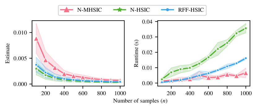
Figure 1: Estimation accuracy for $M=2$ components; the theoretical HSIC value is zero.

Dependent Data ($H_{1}$ holds).

To evaluate the statistical power on $M=2$ components, we set $X_{1}\sim\mathcal{N}(0,1)$, $X_{2}=X_{1}+\epsilon$, and $\epsilon\sim\mathcal{N}(0,1)$, with $n^{\prime}$ set as before. Figure 2 shows that N-MHSIC achieves a power of one for $n\approx 100$ and that it is slightly worse than the existing HSIC approximations for small sample sizes. V-HSIC has the highest power but also the highest runtime. Even though NFSIC has linear runtime complexity it is slower than all other statistics on small sample sizes.

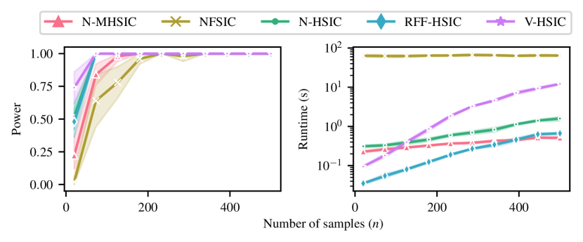
Figure 2: Power on dependent data. Runtime on log scale.

Causal Discovery.

The experiments until now considered $M=2$ components. However, N-MHSIC allows for handling $M\geq 2$ components and thus can estimate the directed acyclic graph (DAG) governing causality if one assumes an additive noise model.

Specifically, we sample from the structural equations $X_{i}=\sum_{j\in\mathrm{PA}_{i}}f^{i,j}\left(X_{j}\right)+\epsilon_{i}$ for $i\in[M]$, of a randomly selected fully connected DAG with four nodes ($M=4$), of which there are $24$. In the equation, $\mathrm{PA}_{i}$ denotes the parents of $i$ in the associated DAG, and the $\epsilon_{i}$ are normally distributed and jointly independent, with a variance sampled independently from the uniform distribution $\mathcal{U}\left(1,\sqrt{2}\right)$.

To now test whether a particular DAG fits the data, Pfister et al. [2018] propose to use generalized additive model regression to find the residuals when regressing each node onto all its parents and to reject the DAG if the residuals are not jointly independent. If these are independent, we accept the causal structure. In this application, one is only interested in the relative $p$-values when performing the procedure for all possible DAGs with the correct number of nodes.

V-HSIC has the best performance in [Pfister et al., 2018], so we only compare against V-HSIC; it is also the only other approach which allows testing joint independence of more than two components. Figure 3 shows how often N-MHSIC and V-HSIC identify the correct DAG in 100 samples. V-HSIC has higher power than N-MHSIC and more often identifies the correct DAG for small sample sizes. However, as the r.h.s. of Figure 3 shows, the proposed algorithm runs even for $n^{\prime}=8\sqrt{n}$ and $n=1500$ twice as fast as V-HSIC while producing the same result quality. Due to their different runtime complexities, the gap in runtime widens further with increasing sample size.

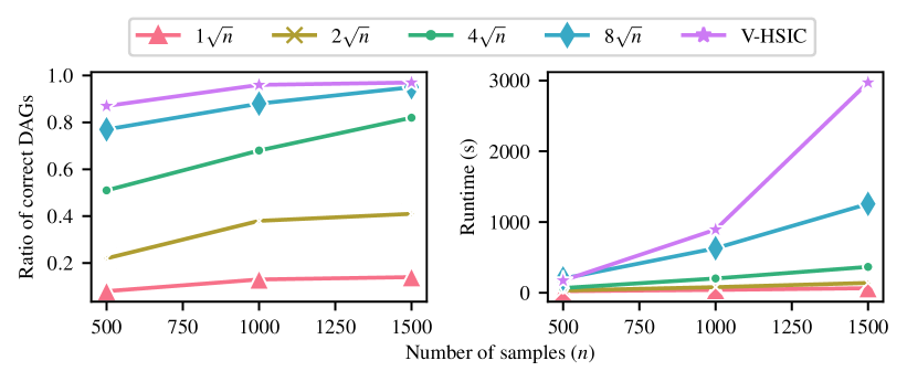
Figure 3: Ratio of correctly identified DAGs with $4$ nodes.

5.2 Real-World Data

This section is dedicated to benchmarks on real-world data.

Million Song Data. The Million Song Data [Bertin-Mahieux et al., 2011] contains approximately 500,000 songs. Each has 90 features ($X$) together with its year of release, which ranges from 1922 to 2011 ($Y$). The algorithms must detect the dependence between the features and the year of release. To approximate the power, we draw $100$ independent samples of the whole data set. Figure 4 shows the results, for level $\alpha=0.01$; the different ranges of $n$ highlight the asymptotic runtime gains. In contrast to a similar experiment of Jitkrittum et al. [2017], we use a permutation approach for all two-sample tests and increase the number of Nyström samples (random Fourier features) as a function of $n$, obtaining higher power throughout. The problem is sufficiently challenging, so that we set the number of Nyström samples to $8\sqrt{n}$ for N-MHSIC. V-HSIC and NFSIC achieve maximum power from $n=500$. N-MHSIC features similar runtime and power as the existing HSIC approximations N-HSIC and RFF-HSIC but can handle more than two components. The runtime plot illustrates that the lower asymptotic complexity of N-MHSIC compared to V-HSIC also holds in practice.

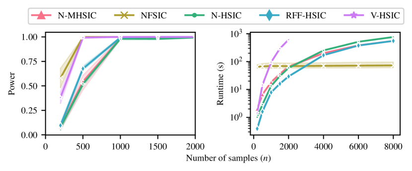
Figure 4: Test power vs. runtime on the Million Song Data.

Weather Causal Discovery.

Here, we aim to infer the correct causality DAG from real-world data, namely the data set of Mooij et al. [2016] which contains $349$ measurements consisting of altitude, temperature and sunshine. The goal is to infer the most plausible DAG with three nodes $(d=3)$ out of the $25$ possible DAGs ($3^{3}-2=25$; two graphs have a cycle). We assume the structural equations discussed before. Figure 5 shows the $p$-values with the estimated DAG (with index $25$) having the largest $p$-value. Again, we compare our results to V-HSIC and find that both successfully identify the most plausible DAG [Pfister et al., 2018].

These experiments demonstrate the efficiency of the proposed Nyström $M$-HSIC method.

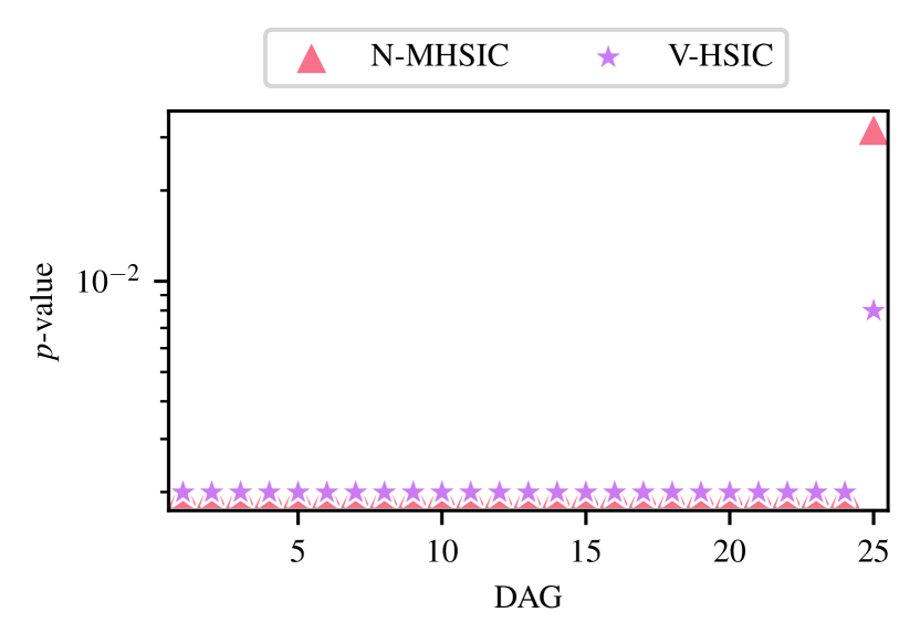
Figure 5: Testing for joint independence on the residuals of DAGs with three nodes (left) and the DAG with the largest $p$-value (right). The $p$-values agree on DAGs $1$ to $24$.

Appendix A Appendix

Section A.1 contains two external theorems and lemmas that we use. Section A.2 is about our proofs.

A.1 External Theorems and Lemmas

In this section two theorems and lemmas are recalled for self-completeness, Theorem A.1 is about bounding the error of Nyström mean embeddings [Chatalic et al., 2022, Theorem 4.1], Theorem A.2 is a well-known result [Serfling, 1980, Section 5.6, Theorem A] for bounding the deviation of U-statistics. Lemma A.1 is about connection between U- and V-statistics. Lemma A.2 recalls Markov’s inequality.

Theorem A.1 (Bound on mean embeddings).

Let $\mathcal{X}$ be a locally compact second-countable topological space, $X$ a random variable supported on $\mathcal{X}$ with Borel probability measure $\mathbb{P}{}$, and let $\mathcal{H}_{k}$ be a RKHS on $\mathcal{X}$ with kernel $k:\mathcal{X}\times\mathcal{X}\to\mathbb{R}$, and feature map $\phi_{k}$. Assume that there exists a constant $K\in(0,\infty)$ such that $\sup_{x\in\mathcal{X}}\sqrt{k(x,x)}\leq K$. Let $C_{k}=\mathbb{E}\left[\phi_{k}(X)\otimes\phi_{k}(X)\right]$. Furthermore, assume that the data points $\hat{\mathbb{P}}_{n}=\{x_{1},\dots,x_{n}\}$ are drawn i.i.d. from the distribution $\mathbb{P}{}$ and that $n^{\prime}\leq n$ subsamples $\tilde{\mathbb{P}}_{n^{\prime}}=\{\tilde{x}_{1},\dots,\tilde{x}_{n^{\prime}}\}$ are drawn uniformly with replacement from the dataset $\hat{\mathbb{P}}_{n}$. Then for any $\delta\in(0,1)$ it holds that

$$\left\|{\mu_{k}\left(\mathbb{P}{}\right)-\mu_{k}\left(\tilde{\mathbb{P}}_{n^{\prime}}\right)}\right\|_{\mathcal{H}_{k}}\leq\frac{c_{1}}{\sqrt{n}}+\frac{c_{2}}{n^{\prime}}+\frac{c_{3}\sqrt{\log(n^{\prime}/\delta)}}{n^{\prime}}\sqrt{\mathcal{N}_{X}\left(\frac{12K^{2}\log(n^{\prime}/\delta)}{n^{\prime}}\right)},$$

with probability at least $1-\delta$ provided that

$$n^{\prime}\geq\max\left(67,12K^{2}\left\|{C_{k}}\right\|_{\mathrm{op}}^{-1}\right)\log\left(\frac{n^{\prime}}{\delta}\right),$$

where $c_{1}=2K\sqrt{2\log(6/\delta)}$, $c_{2}=4\sqrt{3}K\log(12/\delta)$, and $c_{3}=12\sqrt{3\log(12/\delta)}K$.

Recall that a U-statistic is the average of a (symmetric) core function $h=h(x_{1},\dots,x_{m})$ over the observations $X_{1},\dots,X_{n}\sim\mathbb{P}$ ($n\geq m$) with form

$$U_{n}=U(X_{1},\dots,X_{m})=\frac{1}{\binom{n}{m}}\sum_{c}h(X_{i_{1}},\dots,X_{i_{m}}),$$ (21)

where $c$ is the set of the $\binom{n}{m}$ combinations of $m$ distinct elements $\{i_{1},\dots,i_{m}\}$ from $\{1,\dots,n\}$. $U_{n}$ is an unbiased estimator of $\theta=\theta(\mathbb{P})=\mathbb{E}_{\mathbb{P}}[h(X_{1},\dots,X_{m})]$.

Theorem A.2 (Hoeffding’s inequality for U-statistics).

Let $h=h(x_{1},\dots,x_{m})$ be a core function for $\theta=\theta(\mathbb{P})=\mathbb{E}_{\mathbb{P}}\left[h(X_{1},\dots,X_{m})\right]$ with $a\leq h(x_{1},\dots,x_{m})\leq b$. Then, for any $u>0$ and $n\geq m$,

$$\mathbb{P}(U_{n}-\theta\geq u)\leq\exp\left(-\frac{2nu^{2}}{m(b-a)^{2}}\right).$$

Similar to (21) one can consider an alternative (slightly biased) estimator of $\theta$, which is called V-statistic:

$$V_{n}=V(X_{1},\dots,X_{m})=\frac{1}{{n}^{m}}\sum_{(i_{1},\dots,i_{m})\in T_{m}(n)}h(X_{i_{1}},\dots,X_{i_{m}}),$$ (22)

where $T_{m}(n)$ is the $m$-fold Cartesian product of the set $[n]$.

There is a close relation between U- and V-statistics, as it is made explicit by the following lemma [Serfling, 1980, Lemma, Section 5.7.3].

Lemma A.1 (Connection between U- and V-statistics).

Let $\mathbb{P}$ be a probability measure on a metric space $\mathcal{X}$. Let $(X_{i})_{i\in[n]}\stackrel{{\scriptstyle\text{i.i.d.}}}{{\sim}}\mathbb{P}$. Let $m$ denote any element of $[n]$. Let $h$ be a core function satisfying $\mathbb{E}\left[|h(X_{1},\dots,X_{m})|^{r}\right]<\infty$ with some $r\in\mathbb{Z}_{+}$. Let $U_{n}$ and $V_{n}$ denote the U and V-statistic associated to $h$ as defined in (21) and (22), respectively. Then it holds that

$$\mathbb{E}\left[\left|U_{n}-V_{n}\right|^{r}\right]=\mathcal{O}\left(n^{-r}\right).$$

Lemma A.2 (Markov inequality).

For a real-valued random variable $X$ with probability distribution $\mathbb{P}$ and $a>0$, it holds that

$$\mathbb{P}\left(|X|\geq a\right)\leq\frac{\mathbb{E}\left(|X|\right)}{a}.$$

A.2 Proofs

This section is dedicated to proofs. Lemma 4.2 is derived in Section A.2.1. Proposition 4.1 is proved in Section A.2.3 relying on two lemmas shown in Section A.2.2. Lemma 4.4 is proved in Section A.2.5, with an auxiliary result in Section A.2.4.

A.2.1 Proof of Lemma 4.2

Let $\mu_{k}\left(\tilde{\mathbb{P}}_{n^{\prime}}\right)=\sum_{i=1}^{n^{\prime}}\alpha_{k}^{i}\otimes_{m=1}^{M}\phi_{k_{m}}(x_{m}^{i})$, and let $\mu_{k_{m}}\left(\tilde{\mathbb{P}}_{m,n^{\prime}}\right)=\sum_{i=1}^{n^{\prime}}\alpha_{k_{m}}^{i}\phi_{k_{m}}(x_{m}^{i})$ for $m\in[M]$. We write

$$\operatorname{HSIC}_{k,\text{N}}^{2}\left(\hat{\mathbb{P}}_{n}\right) =\left\|{\mu_{k}\left(\tilde{\mathbb{P}}_{n^{\prime}}\right)-\otimes_{m=1}^{M}\mu_{k_{m}}\left(\tilde{\mathbb{P}}_{m,n^{\prime}}\right)}\right\|_{\mathcal{H}_{k}}^{2}$$

$$=\underbrace{\left\|{\mu_{k}\left(\tilde{\mathbb{P}}_{n^{\prime}}\right)}\right\|_{\mathcal{H}_{k}}^{2}}_{=:A}-2\cdot\underbrace{\left\langle\mu_{k}\left(\tilde{\mathbb{P}}_{n^{\prime}}\right),\otimes_{m=1}^{M}\mu_{k_{m}}\left(\tilde{\mathbb{P}}_{m,n^{\prime}}\right)\right\rangle_{\mathcal{H}_{k}}}_{=:C}+\underbrace{\left\|{\otimes_{m=1}^{M}\mu_{k_{m}}\left(\tilde{\mathbb{P}}_{m,n^{\prime}}\right)}\right\|_{\mathcal{H}_{k}}^{2}}_{=:B},$$

and continue term-by-term. Using the definition of the tensor product, we have for term $A$ that

$$A =\left\langle\mu_{k}\left(\tilde{\mathbb{P}}_{n^{\prime}}\right),\mu_{k}\left(\tilde{\mathbb{P}}_{n^{\prime}}\right)\right\rangle_{\mathcal{H}_{k}}=\sum_{i=1}^{n^{\prime}}\sum_{j=1}^{n^{\prime}}\alpha_{k}^{i}\alpha_{k}^{j}\left\langle\otimes_{m=1}^{M}\phi_{k_{m}}(x_{m}^{i}),\otimes_{m=1}^{M}\phi_{k_{m}}(x_{m}^{j})\right\rangle_{\mathcal{H}_{k}}=\sum_{i=1}^{n^{\prime}}\sum_{j=1}^{n^{\prime}}\alpha_{k}^{i}\alpha_{k}^{j}\prod_{m=1}^{M}k_{m}(x_{m}^{i},x_{m}^{j})$$

$$=\bm{\alpha}_{k}^{\mkern-1.5mu\mathsf{T}}\left(\operatorname{\circ}_{m=1}^{M}\mathbf{K}_{k_{m}}\right)\bm{\alpha}_{k}.$$

Similarly, we obtain for term $B$ that

$$B =\left\langle\otimes_{m=1}^{M}\mu_{k_{m}}\left(\tilde{\mathbb{P}}_{m,n^{\prime}}\right),\otimes_{m=1}^{M}\mu_{k_{m}}\left(\tilde{\mathbb{P}}_{m,n^{\prime}}\right)\right\rangle_{\mathcal{H}_{k}}$$

$$=\left\langle\otimes_{m=1}^{M}\sum_{i^{(m)}=1}^{n^{\prime}}\alpha_{k_{m}}^{i^{(m)}}\phi_{k_{m}}\left(x_{m}^{i^{(m)}}\right),\otimes_{m=1}^{M}\sum_{j^{(m)}=1}^{n^{\prime}}\alpha_{k_{m}}^{j^{(m)}}\phi_{k_{m}}\left(x_{m}^{j^{(m)}}\right)\right\rangle_{\mathcal{H}_{k}}$$

$$\stackrel{{\scriptstyle(*)}}{{=}}\prod_{m=1}^{M}\sum_{i^{(m)}=1}^{n^{\prime}}\sum_{j^{(m)}=1}^{n^{\prime}}\alpha_{k_{m}}^{i^{(m)}}\alpha_{k_{m}}^{j^{(m)}}k_{m}\left(x_{m}^{i^{(m)}},x_{m}^{j^{(m)}}\right)=\prod_{m=1}^{M}\bm{\alpha}_{k_{m}}^{\mkern-1.5mu\mathsf{T}}\mathbf{K}_{k_{m}}\bm{\alpha}_{k_{m}},$$

where in $(*)$ we used (1), the linearity of the inner product, and the reproducing property.

Last, we express term $C$ as

$$C =\left\langle\sum_{i=1}^{n^{\prime}}\alpha_{k}^{i}\otimes_{m=1}^{M}\phi_{k_{m}}\left(x_{m}^{i}\right),\otimes_{m=1}^{M}\sum_{j^{(m)}=1}^{n^{\prime}}\alpha_{k_{m}}^{j^{(m)}}\phi_{k_{m}}\left(x_{m}^{j^{(m)}}\right)\right\rangle_{\mathcal{H}_{k}}$$

$$\stackrel{{\scriptstyle(a)}}{{=}}\sum_{i=1}^{n^{\prime}}\alpha_{k}^{i}\left\langle\otimes_{m=1}^{M}\phi_{k_{m}}\left(x_{m}^{i}\right),\otimes_{m=1}^{M}\sum_{j^{(m)}=1}^{n^{\prime}}\alpha_{k_{m}}^{j^{(m)}}\phi_{k_{m}}\left(x_{m}^{j^{(m)}}\right)\right\rangle_{\mathcal{H}_{k}}$$

$$\stackrel{{\scriptstyle(b)}}{{=}}\sum_{i=1}^{n^{\prime}}\alpha_{k}^{i}\prod_{m\in[M]}\left\langle\phi_{k_{m}}\left(x_{m}^{i}\right),\sum_{j^{(m)}=1}^{n^{\prime}}\alpha_{k_{m}}^{j^{(m)}}\phi_{k_{m}}\left(x_{m}^{j^{(m)}}\right)\right\rangle_{\mathcal{H}_{k}}$$

$$\stackrel{{\scriptstyle(c)}}{{=}}\sum_{i=1}^{n^{\prime}}\alpha_{k}^{i}\prod_{m\in[M]}\sum_{j^{(m)}=1}^{n^{\prime}}\alpha_{k_{m}}^{j^{(m)}}\left\langle\phi_{k_{m}}\left(x_{m}^{i}\right),\phi_{k_{m}}\left(x_{m}^{j^{(m)}}\right)\right\rangle_{\mathcal{H}_{k}}$$

$$\stackrel{{\scriptstyle(d)}}{{=}}\sum_{i=1}^{n^{\prime}}\alpha_{k}^{i}\prod_{m\in[M]}\underbrace{\sum_{j^{(m)}=1}^{n^{\prime}}\alpha_{k_{m}}^{j^{(m)}}k_{m}\left(x_{m}^{i},x_{m}^{j^{(m)}}\right)}_{\left(\mathbf{K}_{k_{m}}\right)_{i}\bm{\alpha}_{k_{m}}}=\bm{\alpha}_{k}^{\mkern-1.5mu\mathsf{T}}\left(\operatorname{\circ}_{m=1}^{M}\mathbf{K}_{k_{m}}\bm{\alpha}_{k_{m}}\right),$$

where (a) follows from the linearity of the inner product, (b) holds by (1), (c) is implied by the linearity of the inner product, (d) is valid by the reproducing property, and we refer to the $i$-th row of $\mathbf{K}_{k_{m}}$ as $\left(\mathbf{K}_{k_{m}}\right)_{i}$.

Substituting terms $A,B$, and $C$ concludes the proof.

A.2.2 Two Lemmas to the Proof of Proposition 4.1

Our main result relies on two lemmas.

Lemma A.3 (Error bound for Nyström mean embedding of tensor product kernel).

Let $X=(X_{m})_{m=1}^{M}\in\mathcal{X}=\times_{m=1}^{M}\mathcal{X}_{m}$, $X\sim\mathbb{P}{}\in\mathcal{M}_{1}^{+}(\mathcal{X}{})$, and $(\mathcal{X}_{m})_{m\in[M]}$ locally compact, second-countable topological spaces. Let $k_{m}:\mathcal{X}_{m}\times\mathcal{X}_{m}\rightarrow\mathbb{R}$ be a bounded kernel, i.e. there exists $a_{k_{m}}\in(0,\infty)$ such that $\sup_{x_{m}\in\mathcal{X}_{m}}\sqrt{k_{m}(x_{m},x_{m})}\leq a_{k_{m}}$ for $m\in[M]$. Let $a_{k}=\prod_{m=1}^{M}a_{k_{m}}$, $k=\otimes_{m=1}^{M}k_{m}$, $\mathcal{H}_{k}$ the RKHS associated to $k$, $\phi_{k}=\otimes_{m=1}^{M}\phi_{k_{m}}$, $C_{k}=\mathbb{E}\left[\phi_{k}(X)\otimes\phi_{k}(X)\right]$, $n^{\prime}\leq n$, and $\tilde{\mathbb{P}}_{n^{\prime}}$ defined according to (14). Then for any $\delta\in(0,1)$ it holds that

$$\left\|{\mu_{k}\left(\mathbb{P}{}\right)-\mu_{k}\left(\tilde{\mathbb{P}}_{n^{\prime}}\right)}\right\|_{\mathcal{H}_{k}}\leq\frac{c_{k,1}}{\sqrt{n}}+\frac{c_{k,2}}{n^{\prime}}+\frac{c_{k,3}\sqrt{\log(n^{\prime}/\delta)}}{n^{\prime}}\sqrt{\mathcal{N}_{X}\left(\frac{12a_{k}^{2}\log(n^{\prime}/\delta)}{n^{\prime}}\right)},$$

with probability at least $1-\delta$, provided that

$$n^{\prime}\geq\max\left(67,12a_{k}^{2}\left\|{C_{k}}\right\|_{\mathrm{op}}^{-1}\right)\log\left(\frac{n^{\prime}}{\delta}\right),$$

where $c_{k,1}=2a_{k}\sqrt{2\log(6/\delta)}$, $c_{k,2}=4\sqrt{3}a_{k}\log(12/\delta)$, and $c_{k,3}=12\sqrt{3\log(12/\delta)}a_{k}$.

Proof.

With $\mathcal{X}=\times_{m\in[M]}\mathcal{X}_{m}$, noticing that $\mathcal{X}$ is locally compact second-countable iff. $(\mathcal{X}_{m})_{m\in[M]}$ are so [Willard, 1970, Theorem 16.2(c), Theorem 18.6], $\mathcal{H}_{k}=\otimes_{m=1}^{M}\mathcal{H}_{k_{m}}$, $\phi_{k}=\otimes_{m=1}^{M}\phi_{k_{m}}$, and $\sqrt{k(x,x)}=\prod_{m=1}^{M}\sqrt{k_{m}(x_{m},x_{m})}\leq a_{k}$, the statement is implied by Theorem A.1. ∎

Proof of Lemma 4.3.

To simplify notation, let $\mu_{k_{m}}=\mu_{k_{m}}\left(\mathbb{P}_{m}\right)$, $\tilde{\mu}_{k_{m}}=\mu_{k_{m}}\left(\tilde{\mathbb{P}}_{m,n^{\prime}}\right)$, $\mathcal{H}_{k}=\otimes_{m=1}^{M}\mathcal{H}_{k_{m}}$, and $d_{k_{m}}=\left\|{\mu_{k_{m}}-\tilde{\mu}_{k_{m}}}\right\|_{\mathcal{H}_{k_{m}}}$. The proof proceeds by induction on $M$: For $M=1$ the l.h.s. = r.h.s. = $\left\|{\mu_{k_{1}}\left(\mathbb{P}_{1}\right)-\mu_{k_{1}}\left(\tilde{\mathbb{P}}_{1,n^{\prime}}\right)}\right\|_{\mathcal{H}_{k}}$ is satisfied, and we assume that the statement holds for $M=M-1$, to obtain

$$\left\|{\otimes_{m=1}^{M}\mu_{k_{m}}-\otimes_{m=1}^{M}\tilde{\mu}_{k_{m}}}\right\|_{\mathcal{H}_{k}}=\big{\|}\otimes_{m=1}^{M}\mu_{k_{m}}-\otimes_{m=1}^{M-1}\mu_{k_{m}}\otimes\tilde{\mu}_{k_{M}}+\otimes_{m=1}^{M-1}\mu_{k_{m}}\otimes\tilde{\mu}_{k_{M}}-\otimes_{m=1}^{M}\tilde{\mu}_{k_{m}}\big{\|}_{\mathcal{H}_{k}}$$

$$=\left\|\otimes_{m=1}^{M-1}\mu_{k_{m}}\otimes(\mu_{k_{M}}-\tilde{\mu}_{k_{M}})\right.+\left.\left(\otimes_{m=1}^{M-1}\mu_{k_{m}}-\otimes_{m=1}^{M-1}\tilde{\mu}_{k_{m}}\right)\otimes\tilde{\mu}_{k_{M}}\right\|_{\mathcal{H}_{k}}$$

$$\stackrel{{\scriptstyle(a)}}{{\leq}}\left\|\otimes_{m=1}^{M-1}\mu_{k_{m}}\otimes(\mu_{k_{M}}-\tilde{\mu}_{k_{M}})\right\|_{\mathcal{H}_{k}}+\left\|\left(\otimes_{m=1}^{M-1}\mu_{k_{m}}-\otimes_{m=1}^{M-1}\tilde{\mu}_{k_{m}}\right)\otimes\tilde{\mu}_{k_{M}}\right\|_{\mathcal{H}_{k}}$$

$$\stackrel{{\scriptstyle(b)}}{{=}}\left(\prod_{m\in[M-1]}\left\|\mu_{k_{m}}\right\|_{\mathcal{H}_{k_{m}}}\right)d_{k_{M}}+\left\|\otimes_{m=1}^{M-1}\mu_{k_{m}}-\otimes_{m=1}^{M-1}\tilde{\mu}_{k_{m}}\right\|_{\otimes_{m=1}^{M-1}\mathcal{H}_{k_{m}}}\left\|\tilde{\mu}_{k_{M}}\right\|_{\mathcal{H}_{k_{M}}}$$

$$\stackrel{{\scriptstyle(c)}}{{\leq}}d_{k_{M}}\prod_{m\in[M-1]}a_{k_{m}}+\left\|\otimes_{m=1}^{M-1}\mu_{k_{m}}-\otimes_{m=1}^{M-1}\tilde{\mu}_{k_{m}}\right\|_{\otimes_{m=1}^{M-1}\mathcal{H}_{k_{m}}}\left(a_{k_{M}}+d_{k_{M}}\right)$$

$$\stackrel{{\scriptstyle(d)}}{{\leq}}d_{k_{M}}\prod_{m\in[M-1]}a_{k_{m}}+\left\{\prod_{m\in[M-1]}\left(a_{k_{m}}+d_{k_{m}}\right)-\prod_{m\in[M-1]}a_{k_{m}}\right\}\left(a_{k_{M}}+d_{k_{M}}\right)$$

$$=d_{k_{M}}\prod_{m\in[M-1]}a_{k_{m}}+\prod_{m\in[M]}\left(a_{k_{m}}+d_{k_{m}}\right)-\prod_{m\in[M]}a_{k_{m}}-d_{k_{M}}\prod_{m\in[M-1]}a_{k_{m}}$$

$$=\prod_{m\in[M]}\left(a_{k_{m}}+d_{k_{m}}\right)-\prod_{m\in[M]}a_{k_{m}},$$

where (a) holds by the triangle inequality, (b) is implied by (2) and the definition of $d_{k_{M}}$, (c) follows from

$$\left\|\mu_{k_{m}}\right\|_{\mathcal{H}_{k_{m}}} =\left\|\int_{\mathcal{X}_{m}}k_{m}(\cdot,x_{m})\mathrm{d}\mathbb{P}_{m}(x_{m})\right\|_{\mathcal{H}_{k_{m}}}\stackrel{{\scriptstyle(e)}}{{\leq}}\int_{\mathcal{X}_{m}}\underbrace{\left\|k_{m}(\cdot,x_{m})\right\|_{\mathcal{H}_{k_{m}}}}_{\stackrel{{\scriptstyle(f)}}{{=}}\sqrt{k_{m}(x_{m},x_{m})}\stackrel{{\scriptstyle(g)}}{{\leq}}a_{k_{m}}}\mathrm{d}\mathbb{P}_{m}(x_{m})\leq a_{k_{m}},$$ (23)

$$\left\|{\tilde{\mu}_{k_{M}}}\right\|_{\mathcal{H}_{k_{M}}} =\left\|{\tilde{\mu}_{k_{M}}-\mu_{k_{M}}+\mu_{k_{M}}}\right\|_{\mathcal{H}_{k_{M}}}\stackrel{{\scriptstyle(h)}}{{\leq}}\left\|{\tilde{\mu}_{k_{M}}-\mu_{k_{M}}}\right\|_{\mathcal{H}_{k_{M}}}+\left\|{\mu_{k_{M}}}\right\|_{\mathcal{H}_{k_{M}}}\stackrel{{\scriptstyle(i)}}{{\leq}}d_{k_{M}}+a_{k_{M}},$$

(d) is valid by the induction statement holding for $M-1$, (e) is a property of Bochner integrals, (f) is implied by the reproducing property, (g) comes from the definition of $a_{k_{m}}$, the triangle inequality implies (h), (i) follows from (23) and the definition of $d_{k_{M}}$. ∎

A.2.3 Proof of Proposition 4.1

Let $k=\otimes_{m=1}^{M}k_{m}$, and let $\mathcal{H}_{k}=\otimes_{m=1}^{M}\mathcal{H}_{k_{m}}$. We note that $\mathcal{X}=\times_{m\in[M]}\mathcal{X}_{m}$ is locally compact second-countable as $(\mathcal{X}_{m})_{m\in[M]}$ are so [Willard, 1970, Theorem 16.2(c), Theorem 18.6].

We decompose the error of the Nyström approximation as

$$\left|\mathrm{HSIC}_{k}(\mathbb{P}{})-\operatorname{HSIC}_{k,\text{N}}\left(\hat{\mathbb{P}}_{n}\right)\right| =\left|\left\|{\mu_{k}(\mathbb{P}{})-\otimes_{m=1}^{M}\mu_{k_{m}}(\mathbb{P}_{m})}\right\|_{\mathcal{H}_{k}}-\left\|{\mu_{k}\left(\tilde{\mathbb{P}}_{n^{\prime}}\right)-\otimes_{m=1}^{M}\mu_{k_{m}}\left(\tilde{\mathbb{P}}_{m,n^{\prime}}\right)}\right\|_{\mathcal{H}_{k}}\right|$$

$$\stackrel{{\scriptstyle(a)}}{{\leq}}\left\|{\mu_{k}(\mathbb{P}{})-\otimes_{m=1}^{M}\mu_{k_{m}}(\mathbb{P}_{m})-\mu_{k}\left(\tilde{\mathbb{P}}_{n^{\prime}}\right)+\otimes_{m=1}^{M}\mu_{k_{m}}\left(\tilde{\mathbb{P}}_{m,n^{\prime}}\right)}\right\|_{\mathcal{H}_{k}}$$

$$\stackrel{{\scriptstyle(b)}}{{\leq}}\underbrace{\left\|{\mu_{k}(\mathbb{P}{})-\mu_{k}\left(\tilde{\mathbb{P}}_{n^{\prime}}\right)}\right\|_{\mathcal{H}_{k}}}_{t_{1}}+\underbrace{\left\|{\otimes_{m=1}^{M}\mu_{k_{m}}(\mathbb{P}_{m})-\otimes_{m=1}^{M}\mu_{k_{m}}\left(\tilde{\mathbb{P}}_{m,n^{\prime}}\right)}\right\|_{\mathcal{H}_{k}}}_{t_{2}},$$

where (a) holds by the reverse triangle inequality, and (b) follows from the triangle inequality.

First term ($t_{1}$): One can bound the error of the first term by Lemma A.3; in other words, for any $\delta\in(0,1)$ with probability at least $(1-\delta)$ it holds that

$$\left\|{\mu_{k}(\mathbb{P}{})-\mu_{k}\left(\tilde{\mathbb{P}}_{n^{\prime}}\right)}\right\|_{\mathcal{H}_{k}}\leq\frac{c_{k,1}}{\sqrt{n}}+\frac{c_{k,2}}{n^{\prime}}+\frac{c_{k,3}\sqrt{\log(n^{\prime}/\delta)}}{n^{\prime}}\sqrt{\mathcal{N}_{X_{m}}\left(\frac{12a_{k_{m}}^{2}\log(n^{\prime}/\delta)}{n^{\prime}}\right)}$$

provided that $n^{\prime}\geq\max\left(67,12a_{k}^{2}\left\|{C_{k}}\right\|_{\mathrm{op}}^{-1}\right)\log\left(\frac{n^{\prime}}{\delta}\right)$, with the constants $c_{k,1}=2a_{k}\sqrt{2\log(6/\delta)}$, $c_{k,2}=4\sqrt{3}a_{k}\log(12/\delta)$, $c_{k,3}=12\sqrt{3\log(12/\delta)}a_{k}$.

Second term ($t_{2}$): Applying Lemma 4.3 to the second term gives

$$\left\|{\otimes_{m=1}^{M}\mu_{k_{m}}(\mathbb{P}_{m})-\otimes_{m=1}^{M}\mu_{k_{m}}\left(\tilde{\mathbb{P}}_{m,n^{\prime}}\right)}\right\|_{\mathcal{H}_{k}} \leq\prod_{m\in[M]}\left(a_{k_{m}}+\left\|{\mu_{k_{m}}\left(\mathbb{P}_{m}\right)-\mu_{k_{m}}\left(\tilde{\mathbb{P}}_{m,n^{\prime}}\right)}\right\|_{\mathcal{H}_{k_{m}}}\right)-\prod_{m\in[M]}a_{k_{m}}.$$

We now bound the error of each of the $M$ factors by Theorem A.1, i.e., for fixed $m\in[M]$; particularly we get that for any $\delta\in(0,1)$ with probability at least $1-\delta$

$$\left\|{\mu_{k_{m}}\left(\mathbb{P}_{m}\right)-\mu_{k_{m}}\left(\tilde{\mathbb{P}}_{m,n^{\prime}}\right)}\right\|_{\mathcal{H}_{k_{m}}} \leq\frac{c_{k_{m},1}}{\sqrt{n}}+\frac{c_{k_{m},2}}{n^{\prime}}+\frac{c_{k_{m},3}\sqrt{\log(n^{\prime}/\delta)}}{n^{\prime}}\sqrt{\mathcal{N}_{X_{m}}\left(\frac{12a_{k_{m}}^{2}\log(n^{\prime}/\delta)}{n^{\prime}}\right)},\text{ hence}$$

$$a_{k_{m}}+\left\|{\mu_{k_{m}}\left(\mathbb{P}_{m}\right)-\mu_{k_{m}}\left(\tilde{\mathbb{P}}_{m,n^{\prime}}\right)}\right\|_{\mathcal{H}_{k_{m}}} \leq a_{k_{m}}+\frac{c_{k_{m},1}}{\sqrt{n}}+\frac{c_{k_{m},2}}{n^{\prime}}+\frac{c_{k_{m},3}\sqrt{\log(n^{\prime}/\delta)}}{n^{\prime}}\sqrt{\mathcal{N}_{X_{m}}\left(\frac{12a_{k_{m}}^{2}\log(n^{\prime}/\delta)}{n^{\prime}}\right)},$$

and by union bound that their product is for any $\delta\in(0,\frac{1}{M})$ with probability at least $1-M\delta$

$$\prod_{m\in[M]}\left[a_{k_{m}}+\left\|{\mu_{k_{m}}\left(\mathbb{P}_{m}\right)-\mu_{k_{m}}\left(\tilde{\mathbb{P}}_{m,n^{\prime}}\right)}\right\|_{\mathcal{H}_{k_{m}}}\right]\leq$$

$$\leq\prod_{m\in[M]}\Bigg{[}a_{k_{m}}+\frac{c_{k_{m},1}}{\sqrt{n}}+\frac{c_{k_{m},2}}{n^{\prime}}+\frac{c_{k_{m},3}\sqrt{\log(n^{\prime}/\delta)}}{n^{\prime}}\sqrt{\mathcal{N}_{X_{m}}\left(\frac{12a_{k_{m}}^{2}\log(n^{\prime}/\delta)}{n^{\prime}}\right)}\Bigg{]},$$

$$\prod_{m\in[M]}\left[a_{k_{m}}+\left\|{\mu_{k_{m}}\left(\mathbb{P}_{m}\right)-\mu_{k_{m}}\left(\tilde{\mathbb{P}}_{m,n^{\prime}}\right)}\right\|_{\mathcal{H}_{k_{m}}}\right]-\prod_{m\in[M]}a_{k_{m}}\leq$$

$$\leq\prod_{m\in[M]}\Bigg{[}a_{k_{m}}+\frac{c_{k_{m},1}}{\sqrt{n}}+\frac{c_{k_{m},2}}{n^{\prime}}+\frac{c_{k_{m},3}\sqrt{\log(n^{\prime}/\delta)}}{n^{\prime}}\sqrt{\mathcal{N}_{X_{m}}\left(\frac{12a_{k_{m}}^{2}\log(n^{\prime}/\delta)}{n^{\prime}}\right)}\Bigg{]}-\prod_{m\in[M]}a_{k_{m}},$$

provided that $n^{\prime}\geq\max\left(67,12a_{k_{m}}^{2}\left\|{C_{k_{m}}}\right\|_{\mathrm{op}}^{-1}\right)\log\left(\frac{n^{\prime}}{\delta}\right)$ for all $m\in[M]$, with $C_{k_{m}}=\mathbb{E}\left[\phi_{k_{m}}(X_{m})\otimes\phi_{k_{m}}(X_{m})\right]$ and constants $c_{k_{m},1}=2a_{k_{m}}\sqrt{2\log(6/\delta)}$, $c_{k_{m},2}=4\sqrt{3}a_{k_{m}}\log(12/\delta)$, $c_{k_{m},3}=12\sqrt{3\log(12/\delta)}a_{k_{m}}$, with $m\in[M]$.

Combining the $M+1$ terms by union bound yields the stated result.

A.2.4 Lemma to the Proof of Lemma 4.4

Lemma A.4 (Deviation bound for U-statistics based HSIC estimator).

It holds that

$$\left|\operatorname{HSIC}_{k,u}^{2}\left(\hat{\mathbb{P}}_{n}\right)-\operatorname{HSIC}_{k}^{2}\left(\mathbb{P}\right)\right|=\mathcal{O}_{\text{P}}\left(\frac{1}{\sqrt{n}}\right),$$

where $\operatorname{HSIC}_{k,u}^{2}$ is the U-statistic based estimator of $\operatorname{HSIC}_{k}^{2}$.

Proof.

We show that (3) can be expressed as a sum of U-statistics and then bound the terms individually. First, square (3) to obtain

$$\operatorname{HSIC}_{k}^{2}(\mathbb{P}) =\underbrace{\mathbb{E}_{(x_{1},\dots,x_{M}),(x^{\prime}_{1},\dots,x_{M}^{\prime})\sim\mathbb{P}}\left[\prod_{m\in[M]}k_{m}\left(x_{m},x_{m}^{\prime}\right)\right]}_{A}+\underbrace{\mathbb{E}_{x_{1},x_{1}^{\prime}\sim\mathbb{P}_{1},\dots,x_{M},x_{M}^{\prime}\sim\mathbb{P}_{M}}\left[\prod_{m\in[M]}k_{m}\left(x_{m},x_{m}^{\prime}\right)\right]}_{B}$$

$$\quad\quad-2\underbrace{\mathbb{E}_{(x_{1},\dots,x_{M})\sim\mathbb{P},x_{1}^{\prime}\sim\mathbb{P}_{1},\dots,x_{M}^{\prime}\sim\mathbb{P}_{M}}\left[\prod_{m\in[M]}k_{m}(x_{m},x_{m}^{\prime})\right]}_{C},$$

where $A$, $B$, and $C$ can be estimated by U-statistics $A^{\prime}_{n}$, $B^{\prime}_{n}$, and $C^{\prime}_{n}$, respectively. Let $\operatorname{HSIC}_{k,u}^{2}\left(\hat{\mathbb{P}}_{n}\right)=A^{\prime}_{n}+B^{\prime}_{n}-2C^{\prime}_{n}$, and split $t$ as $\alpha t+\beta t+(1-\alpha-\beta)t$, with $\alpha,\beta>0$ and $\alpha+\beta<1$. One obtains

$$P\left(\left|\operatorname{HSIC}_{k}^{2}(\mathbb{P})-\operatorname{HSIC}_{k,u}^{2}\left(\hat{\mathbb{P}}_{n}\right)\right|\geq t\right)\leq P\left(\left|A-A^{\prime}_{n}\right|\geq\alpha t\right)+P\left(\left|B-B^{\prime}_{n}\right|\geq\beta t\right)+P\left(2\left|C-C^{\prime}_{n}\right|\geq(1-\alpha-\beta)t\right).$$

Doubling and rewriting Theorem A.2, we have that for U-statistics and any $\delta\in(0,1)$

$$\mathbb{P}\left(\left|U_{n}-\theta\right|\geq\sqrt{\frac{m(b-a)^{2}\ln(\frac{2}{\delta})}{2n}}\right)\leq\delta.$$

Now, choosing the $\left(\theta,U_{n},u\right)$ triplet to be $\left(A,A_{n}^{\prime},\alpha t\right)$, $\left(B,B_{n}^{\prime},\beta t\right)$, $\left(C,C_{n}^{\prime},\frac{(1-\alpha-\beta)t}{2}\right)$, respectively, setting $m=2M$, and observing that $a\leq k(x,y)\leq b$ as $k$ is bounded, we obtain that $|A^{\prime}_{n}-A|\sqrt{n}$, $|B^{\prime}_{n}-B|\sqrt{n}$, and $|C^{\prime}_{n}-C|\sqrt{n}$ are bounded in probability and so is their sum. ∎

A.2.5 Proof of Lemma 4.4

We consider the decomposition

$$\left|\operatorname{HSIC}_{k}^{2}\left(\hat{\mathbb{P}}_{n}\right)-\operatorname{HSIC}_{k}^{2}\left(\mathbb{P}\right)\right|\leq\underbrace{\left|\operatorname{HSIC}_{k}^{2}\left(\hat{\mathbb{P}}_{n}\right)-\operatorname{HSIC}_{k,u}^{2}\left(\hat{\mathbb{P}}_{n}\right)\right|}_{t_{1}}+\underbrace{\left|\operatorname{HSIC}_{k,u}^{2}\left(\hat{\mathbb{P}}_{n}\right)-\operatorname{HSIC}^{2}_{k}\left(\mathbb{P}\right)\right|}_{t_{2}},$$ (24)

by using the triangle inequality, where $\operatorname{HSIC}_{k,u}$ is the U-statistic based HSIC estimator.

Second term ($t_{2}$): Lemma A.4 establishes that $t_{2}=\mathcal{O}_{\text{P}}\left(\frac{1}{\sqrt{n}}\right)$.

First term ($t_{1}$): To bound $t_{1}$, first, by Markov’s inequality (Lemma A.2) observe that

$$\mathbb{P}\left(\left|\operatorname{HSIC}_{k}^{2}\left(\hat{\mathbb{P}}_{n}\right)-\operatorname{HSIC}_{k,u}^{2}\left(\hat{\mathbb{P}}_{n}\right)\right|\geq a\right) \leq\underbrace{\frac{\mathbb{E}\left(\left|\operatorname{HSIC}_{k}^{2}\left(\hat{\mathbb{P}}_{n}\right)-\operatorname{HSIC}_{k,u}^{2}\left(\hat{\mathbb{P}}_{n}\right)\right|\right)}{a}}_{=:\epsilon},$$

$$\mathbb{P}\left(\left|\operatorname{HSIC}_{k}^{2}\left(\hat{\mathbb{P}}_{n}\right)-\operatorname{HSIC}_{k,u}^{2}\left(\hat{\mathbb{P}}_{n}\right)\right|\geq\frac{\mathbb{E}\left(\left|\operatorname{HSIC}_{k}^{2}\left(\hat{\mathbb{P}}_{n}\right)-\operatorname{HSIC}_{k,u}^{2}\left(\hat{\mathbb{P}}_{n}\right)\right|\right)}{\epsilon}\right) \leq\epsilon,$$

$$\mathbb{P}\left(\left|\operatorname{HSIC}_{k}^{2}\left(\hat{\mathbb{P}}_{n}\right)-\operatorname{HSIC}_{k,u}^{2}\left(\hat{\mathbb{P}}_{n}\right)\right|<\frac{\mathbb{E}\left(\left|\operatorname{HSIC}_{k}^{2}\left(\hat{\mathbb{P}}_{n}\right)-\operatorname{HSIC}_{k,u}^{2}\left(\hat{\mathbb{P}}_{n}\right)\right|\right)}{\epsilon}\right) \geq 1-\epsilon,$$

$$\mathbb{P}\left(\left|\operatorname{HSIC}_{k}^{2}\left(\hat{\mathbb{P}}_{n}\right)-\operatorname{HSIC}_{k,u}^{2}\left(\hat{\mathbb{P}}_{n}\right)\right|<\frac{C}{n\epsilon}\right) \stackrel{{\scriptstyle(*)}}{{\geq}}1-\epsilon,$$

$$\mathbb{P}\left(\left|\operatorname{HSIC}_{k}^{2}\left(\hat{\mathbb{P}}_{n}\right)-\operatorname{HSIC}_{k,u}^{2}\left(\hat{\mathbb{P}}_{n}\right)\right|\geq\frac{C}{n\epsilon}\right) \leq\epsilon,$$ (25)

for constant $C>0$ and $n$ large enough, where $(*)$ follows from Lemma A.1 (with $r=1$). (25) implies that

$$\left|\operatorname{HSIC}_{k}^{2}\left(\hat{\mathbb{P}}_{n}\right)-\operatorname{HSIC}_{k,u}^{2}\left(\hat{\mathbb{P}}_{n}\right)\right|=\mathcal{O}_{\text{P}}\left(\frac{1}{n}\right).$$

Combining the terms ($t_{1}+t_{2}$): Combining the obtained results for the two terms, one gets that

$$\left|\operatorname{HSIC}_{k}^{2}\left(\hat{\mathbb{P}}_{n}\right)-\operatorname{HSIC}_{k}^{2}\left(\mathbb{P}\right)\right| \stackrel{{\scriptstyle\eqref{eq:decompo-1}}}{{\leq}}\left|\operatorname{HSIC}_{k}^{2}\left(\hat{\mathbb{P}}_{n}\right)-\operatorname{HSIC}_{k,u}^{2}\left(\hat{\mathbb{P}}_{n}\right)\right|+\left|\operatorname{HSIC}_{k,u}^{2}\left(\hat{\mathbb{P}}_{n}\right)-\operatorname{HSIC}_{k}^{2}\left(\mathbb{P}\right)\right|$$

$$=\mathcal{O}_{\text{P}}\left(\frac{1}{n}\right)+\mathcal{O}_{\text{P}}\left(\frac{1}{\sqrt{n}}\right)=\mathcal{O}_{\text{P}}\left(\frac{1}{\sqrt{n}}\right).$$ (26)

Hence

$$\mathcal{O}_{\text{P}}\left(\frac{1}{\sqrt{n}}\right) \stackrel{{\scriptstyle\eqref{eq:decompo-2}}}{{\geq}}\left|\operatorname{HSIC}_{k}^{2}\left(\hat{\mathbb{P}}_{n}\right)-\operatorname{HSIC}_{k}^{2}\left(\mathbb{P}\right)\right|=\left|\operatorname{HSIC}_{k}\left(\hat{\mathbb{P}}_{n}\right)-\operatorname{HSIC}_{k}\left(\mathbb{P}\right)\right|\Big{|}\underbrace{\operatorname{HSIC}_{k}\left(\hat{\mathbb{P}}_{n}\right)}_{\stackrel{{\scriptstyle\eqref{eq:emp-hsic}}}{{\geq}}0}+\underbrace{\operatorname{HSIC}_{k}\left(\mathbb{P}\right)}_{\geq 0}\Big{|}$$

$$\geq\left|\operatorname{HSIC}_{k}\left(\hat{\mathbb{P}}_{n}\right)-\operatorname{HSIC}_{k}\left(\mathbb{P}\right)\right|\operatorname{HSIC}_{k}\left(\mathbb{P}\right),$$

which by dividing with the constant $\operatorname{HSIC}_{k}\left(\mathbb{P}\right)>0$ implies the statement.