An application-oriented scheduler

Abstract

We consider a multi-agent system where agents compete for the access to the radio resource. By combining some application-level parameters, such as the resilience, with a knowledge of the radio environment, we propose a new way of modeling the scheduling problem as an optimization problem. We design accordingly a low-complexity solver. The performance are compared with state-of-the-art schedulers via simulations. The numerical results show that this application-oriented scheduler performs better than standard schedulers. As a result, it offers more space for the selection of the application-level parameters to reach any arbitrary performance.

I Introduction

In modern wireless communications, latency and reliability are as important as throughput. Indeed, new applications, such as the industrial internet of things, involve new use cases with very high latency and reliability requirements. For instance, [1] describes latency requirements of 0.5 ms and reliability of 99.999999$\%$ for motion control. Similar figures are provided for mobile automation. These requirements should be met in the context of systems with many agents sharing the same communication resources. Moreover, for agents with different missions, their application requirements and the quality of their channel may vary.

In this scope, we believe that all available degrees of freedom should be used in the design of the communication system. More specifically, the application requirements should be taken into account in the optimization to maximize the performance. Having this paradigm in mind, we shall focus on the critical MAC layer in this paper, namely the scheduling.

Of course, there exist many studies in the literature that propose design guidelines with respect to these new requirements. A relevant emerging field is the Age of Information (AoI). AoI measures the time elapsed between the generation of a message $u(t)$ and its delivery time $t$, i.e., the AoI is $t-u(t)$. This metric enables to assess existing queuing and scheduling strategies and can serve as a design guideline for new algorithms. AoI is a finer metric than the quality of service (QoS), used for resource allocation, e.g. in the LTE [2], as the latter is transmission centric while the former focuses on the quality of the information effectively received. AoI is also different from resource allocation mechanisms considering communication metrics, such as the data rate or the channel capacity, for their scheduling decision [3]. However, the standard AoI metric does not take into account application requirements. It is possible to weight the AoI of each agent (in the case where a sum AoI is optimized) but this does not enable to directly optimize with respect to these requirements. Moreover, according to many definitions a real-time constraint means meeting a deadline. This is slightly different than the metric optimized with AoI.

Related work - In [4], the average time status update with the queue algorithm first-come-first-served is investigated. In [5], the same authors study AoI in the context of a vehicular network. It is shown that the source rate should not be too high to maximize the AoI metric. Moreover, several scheduling algorithms have been proposed to optimize AoI: the AoI in the case of multiple agents, each having multiple sources, and sharing a common channel is considered in [6]. The authors prove that the problem is NP-hard and proposed sub-optimal algorithms. In [7], the case of a base-station delivering information to several agents is studied. The context is similar to the one in this paper, but the optimization is done with respect to a different metric: they investigate a transmission scheduling policy that minimizes the expected weighted sum of the AoI of each agent.

Main contributions - In this work, we define a new multi-agent scheduling problem. It takes several application parameters into account, including the resilience, i.e., how often an application needs to receive fresh information to work properly. This enables to assess the quality of a scheduler with respect to the application failure probability. As a result, similarly to what is done with semantic communications [8], the communication system is optimized directly with respect to its final real-time requirements. We show with numerical evaluations a strong confidence in the proposed scheduler design as the performance gain is significant compared with state-of-art schedulers.

II Context

II-A Description of the system

We consider a discrete-time system, divided in time slots whose length is denoted by $dt$, e.g., $dt=1$ msec. Let $N$ be the number of agents in the system. Any $k^{th}$ agent $A_{k}$ is represented by a data stream characterized by three parameters:

• The period $T$: the time duration between two consecutive packet arrivals from the application in the agent buffer for transmission.

• The packet lifetime $D$ (with $D\leq T$): the time duration for which the packet is alive.

• The resilience $R$: the maximum time duration for which the agent can survive without a successful transmission of a packet.

Fig. 1 shows a representation, called time-line, of $T$ and $D$.

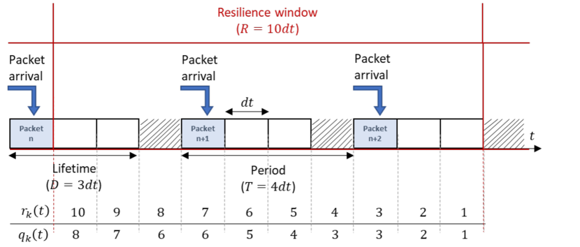
Figure 1: Example of a time-line with $T=4$ and $D=3$ (in number of $dt$’s).

We define the event resilience violation for any agent (E1) as “no packet successfully transmitted during the last $R$ time slots”. For an agent $A_{k}$ at (discrete) time $t$, we accordingly introduce $r_{k}(t)$ as the remaining time before resilience violation. This means that $0\leq r_{k}(t)\leq R$ and $r_{k}(t)$ is a decreasing function of $t$. The complementary event of (E1), called success (E0), is: “successful transmission of a packet at time $t$”. With both the events (E0) and (E1) for any agent $A_{k}$ at time $t$, $r_{k}(t)$ is immediately set to its maximum value $R$.

We define a resilience window as a time window that starts just after one event (E0) or one event (E1), i.e., when $r_{k}(t)=R$, and that ends when $A_{k}$ meets either the next (E0) or the next (E1). Fig. 2 shows an arbitrary example of the time evolution of $r_{k}(t)$ and the associated resilience windows.

Figure 2: Example of a time evolution of $r_{k}(t)$ with $R=10$ (top) and the associated resilience windows (bottom). At time instants $t=7,11,31,33$, $A_{k}$ meets (E0) whereas at time instants $t=22,44$, $A_{k}$ meets (E1).

Additionally, we define a transmission opportunity for an agent $A_{k}$ as a time slot for which a packet is alive. Accordingly, we define the quantity $q_{k}(t)$ as the remaining number of transmission opportunities before meeting (E1). In case $D=T$, i.e., if there is no “hole” in the time-line, then $q_{k}(t)=r_{k}(t)$. In case $D<T$, then $q_{k}(t)\leq r_{k}(t)$.

II-B Description of the environment

We consider a single available radio resource per time slot. We assume that the resource is suited to the transmission of one packet by any agent. Therefore, at any time, all the agents with an alive packet compete for the access to the single radio resource but only one agent finally obtain the resource. We denote by $\delta_{k}(t)=1$ the event “$A_{k}$ is allocated at time $t$” and by $\delta_{k}(t)=0$ the event “$A_{k}$ is not allocated at time $t$”. When allocated the resource, $A_{k}$ observes an unsuccessful transmission of the packet with probability $p_{k}$ being the channel error probability. Thus, an agent $A_{k}$ meets (E1) either if it is never allocated the resource or if the channel strongly impacts the transmission each time the agent is allocated.

II-C Example

Consider a mobile robot with a trajectory monitoring application: $T$ is the time duration between two consecutive position measurements of the agent, $D$ is the time duration for which the measured position remains relevant, and $R$ represents the capacity to interpolate/extrapolate the trajectory without consecutive measurements. We consider that the agent’s mission is to reach a geographical point.

Assume that due to numerous clutters in its surrounding environment, some packets are dropped by the channel resulting in event (E1) for the agent. The trajectory cannot be interpolated/extrapolated with a sufficient accuracy to ensure the success of the mission. Therefore, the agent stops its motion to wait for a full restart which generates, among others, a significant delay. Such an event is then detrimental to the system performance regarding the application purpose.

In our study, for simplification purpose, the restart delay is not considered. In other words, the event (E1) does not stop the agent.

III Optimization problem

In this section, we first formalize the scheduling problem as an optimization problem. Then, we introduce some heuristics to allow for a practical solution.

III-A Presentation of the problem

The problem we propose to solve is the opportunistic centralized scheduling problem: “which agent, at a given time slot, should get the radio ressource given the knowledge of the system and the environment?”. For any agent $A_{k}$ we define $V_{k}(t)$ as the accumulated sum of resilience violations until time $t$. $V_{k}(t)$ is updated based on the events (E0) and (E1) as follows:

Meet (E0): $$V_{k}(t)\leftarrow V_{k}(t-dt),$$ (1)

Meet (E1): $$V_{k}(t)\leftarrow V_{k}(t-dt)+1.$$ (2)

If none of (E0) or (E1) occurs at time $t$, then $V_{k}(t)$ is naturally extended as $V_{k}(t)\leftarrow V_{k}(t-dt)$. From these quantities, we define the local long-term experimented probability of resilience violation at any time $t$ as:

$$F_{k}(t)\stackrel{{\scriptstyle\text{def}}}{{=}}\frac{V_{k}(t)}{t}.$$ (3)

From a system perspective, we define the optimization problem as the search for the scheduling decision $\underline{\delta}^{*}(t)=\{\delta_{1}^{*}(t),...,\delta_{N}^{*}(t)\}$ that minimizes the average probability of resilience violation $F(t)$ embodied by the sum of $F_{k}$’s s.t.:

$$F(t)\stackrel{{\scriptstyle\text{def}}}{{=}}\frac{\sum_{k}V_{k}(t)}{t}.$$ (4)

III-B Proposed alternative objective

As a first step to design an efficient scheduler, we build a heuristic $J\bigl{(}t,\underline{\delta}(t)\bigr{)}$ whose aim is to predict $F(t)$ by predicting actually:

$$S(t)\stackrel{{\scriptstyle\text{def}}}{{=}}\sum_{k}V_{k}(t)$$ (5)

under a given scheduling decision $\underline{\delta}(t)$. The rationale behind considering $S(t)$ instead of $F(t)$ is that $t$ is common to all the agents therefore $t$ only scales the problem, i.e., there is no need to insert it within the optimization problem.

The solver in the following section then consists in choosing the allocation $\underline{\delta}(t)$ such that the heuristic $J\bigl{(}t,\underline{\delta}(t)\bigr{)}$ is minimized. To establish the said heuristic, first, we build a function $\hat{V}\bigl{(}t,\delta_{k}(t)\bigr{)}$ to estimate $V_{k}(t)$ for any agent $A_{k}$. Then, the heuristic $J\bigl{(}t,\underline{\delta}(t)\bigr{)}$ is obtained by summing these local estimates.

III-B1 Local predict function

As $V_{k}(t)$ is an observation metric, we define an associated local long-term predicted accumulated sum of resilience violations $\hat{V}_{k}\bigl{(}t,\delta_{k}(t)\bigr{)}$:

$$\hat{V}_{k}\bigl{(}t,\delta_{k}(t)\bigr{)}\stackrel{{\scriptstyle\text{def}}}{{=}}V_{k}(t-dt)+\hat{f}_{k}\bigl{(}t,\delta_{k}(t)\bigr{)},$$ (6)

where $V_{k}(t-dt)$ is the observed value from the previous time instant and $\hat{f}_{k}\bigl{(}t,\delta_{k}(t)\bigr{)}$ is the local short-term predicted probability of resilience violation within the current resilience window for time $t$ given an allocation decision $\delta_{k}(t)$. The function $\hat{f}_{k}(\cdot,\cdot)$ acts as a correction term especially when $t$ is small. For example, when all $V_{k}$’s are zero at the beginning, they are not well-representing the near future.

We construct $\hat{f}_{k}(\cdot,\cdot)$ to fairly represent the current application status as well as the radio conditions:

• $\hat{f}_{k}(\cdot,\cdot)$ increases as $p_{k}$ increases: a worse radio conditions makes greater the probability of resilience violation

• $\hat{f}_{k}(\cdot,\cdot)$ increases as $r_{k}(t)$ decreases: getting closer to the resilience violation makes greater the probability of resilience violation

We propose the heuristic $f_{r}(\cdot,\cdot)$ that fulfills these requirements

$$f_{r}(t,k)\stackrel{{\scriptstyle\text{def}}}{{=}}p_{k}^{r_{k}(t)}.$$ (7)

In the case of holes in the time-line, i.e., when $D<T$, two agents $A_{k_{1}},A_{k_{2}}$ with the same values $r_{k_{1}}(t)=r_{k_{2}}(t)$ can observe two different time-lines $q_{k_{1}}(t)<q_{k_{2}}(t)$. We propose the following enhancement of the heuristic to distinguish between $A_{k_{1}}$ and $A_{k_{2}}$:

$$f_{q}(t,k)\stackrel{{\scriptstyle\text{def}}}{{=}}p_{k}^{q_{k}(t)}.$$ (8)

Now, we build the function $\hat{f}_{k}(\cdot,\cdot)$ to integrate any of these heuristics. The function should distinguish the case the allocation is not granted from the case the allocation is granted. In the latter case, indeed, $\hat{f}_{k}(\cdot,\cdot)$ must depend on $p_{k}$ because a channel transmission is assumed. As a result, we propose the following definition:

$$\hat{f}_{k}\bigl{(}t,\delta_{k}(t)\bigr{)}=\left\{\begin{array}[]{ll}f(t,k)&\text{if }\delta_{k}(t)=0,\\ p_{k}f(t,k)&\text{if }\delta_{k}(t)=1,\end{array}\right.$$ (9)

where $f$ could be either $f_{r}$ or $f_{q}$. This can be simplified as:

$$\hat{f}_{k}\bigl{(}t,\delta_{k}(t)\bigr{)}=\bigl{(}1-\delta_{k}(t)(1-p_{k})\bigr{)}f(t,k).$$ (10)

Now that $\hat{V}_{k}$ is fully constructed, the local heuristic is nearly completed. We use the utility-based formalism to define the local predict function:

$$j_{k}\bigl{(}t,\delta_{k}(t)\bigr{)}\stackrel{{\scriptstyle\text{def}}}{{=}}U_{\alpha}\Bigl{(}\hat{V}_{k}\bigl{(}t,\delta_{k}(t)\bigr{)}\Bigr{)},$$ (11)

where $U_{\alpha}(\cdot)$ is a non-linear monotonic function identical for all the agents. In this paper, we consider the $\alpha$-fair utility function [9]:

$$U_{\alpha}(x)\stackrel{{\scriptstyle\text{def}}}{{=}}\left\{\begin{array}[]{ll}\frac{x^{1-\alpha}}{1-\alpha}&\alpha\neq 1,\\ \log x&\alpha=1\end{array}\right.,\quad U_{\alpha}^{\prime}(x)=x^{-\alpha}.$$ (12)

The $\alpha$-fair utility framework allows us for considering a family of schedulers with a good performance/fairness tradeoff [10]. The rationale behind the introduction of $U_{\alpha}$ is to stick with such a well-known family of schedulers. Several values of $\alpha$ are considered in this paper to observe if the fairness concern indeed exerts any influence on the scheduling performance.

III-B2 Global predict function

We define the global predict function of $S(t)$ as the sum of the local predict functions:

$$J\bigl{(}t,\underline{\delta}(t)\bigr{)}\stackrel{{\scriptstyle\text{def}}}{{=}}\sum_{k}j_{k}\bigl{(}t,\delta_{k}(t)\bigr{)}.$$ (13)

The goal of the solver is then to find the scheduling decision $\underline{\delta}^{*}(t)$ that minimizes $J$:

$$\underline{\delta}^{*}(t)=\arg\min_{\underline{\delta}(t)}J\bigl{(}t,\underline{\delta}(t)\bigr{)}.$$ (14)

IV Solver

In this section, we present two manners for solving (14): the exact solver and the approximated solver. These two solvers are important regarding the computational complexity because a great number of agents leads the exact solver to overload any computation resource.

IV-A Exact solver for $J$: On-line sum

Let us first compute $j_{k}(t,1)$ and $j_{k}(t,0)$ for any agent $A_{k}$ having an alive packet at time $t$. This corresponds to the events “$A_{k}$ is allocated” and “$A_{k}$ is not allocated”, respectively. If $t$ is a time slot out of the lifetime packet of $A_{k}$, i.e., the packet of $A_{k}$ is dead, $A_{k}$ is not considered for the scheduling decision. $j_{k}(t,1)$ and $j_{k}(t,0)$ are set to infinite values to explicitly exclude $A_{k}$. This provides us Table I.

$k^{*}$	$0$	$1$	$\dots$	$N-1$
$j_{1}\bigl{(}t,\delta_{1}(t)\bigr{)}$	$j_{1}(t,1)$	$j_{1}(t,0)$	$\dots$	$j_{1}(t,0)$
$j_{2}\bigl{(}t,\delta_{2}(t)\bigr{)}$	$j_{2}(t,0)$	$j_{2}(t,1)$	$\dots$	$j_{2}(t,0)$
$\vdots$	$\vdots$	$\vdots$	$\vdots$	$\vdots$
$j_{N}\bigl{(}t,\delta_{N}(t)\bigr{)}$	$j_{N}(t,0)$	$j_{N}(t,0)$	$\dots$	$j_{N}(t,1)$

TABLE I: Table of the on-line sum solver

Secondly, for each scheduler decision, i.e., for each column in Table I, we sum all the rows to obtain a list of $N$ cost values. Thirdly, we extract the column index $k^{*}$ whose cost value is lower than any other cost value. This leads to consider agent $A_{k^{*}}$ as the agent to allocate. This solver requires at least $N$ times the computations of $j_{k}(t,1),j_{k}(t,0)$, then $N$ sums of $N$ terms each (so $N^{2}$ operations at least), then a comparison between $N$ values. Consequently, it might cause computational issues when $N$ increases.

IV-B Approximated solver for $J$: On-line Taylor

For great values of $N$, let us use the Taylor expansion of $U_{\alpha}(\cdot)$ around the prediction $\hat{V}_{k}\bigl{(}t,\delta_{k}(t)\bigr{)}$ considering the experimented $V_{k}(t-dt)$:

$$U_{\alpha}\Bigl{(}\hat{V}_{k}\bigl{(}t,\delta_{k}(t)\bigr{)}\Bigr{)} \approx U_{\alpha}\bigl{(}V_{k}(t-dt)\bigr{)}$$

$$+ \Bigl{(}\hat{V}_{k}\bigl{(}t,\delta_{k}(t)\bigr{)}-V_{k}(t-dt)\Bigr{)}$$

$$\times U_{\alpha}^{\prime}\bigl{(}V_{k}(t-dt)\bigr{)}.$$

We only keep the terms that depend on the current scheduling decision at $t$. In addition, as only one agent is provided the resource at a time, this leads (14) to become:

$$k^{*}=\arg\min_{k}\sum_{k}\hat{V}_{k}\bigl{(}t,\delta_{k}(t)\bigr{)}U_{\alpha}^{\prime}\bigl{(}V_{k}(t-dt)\bigr{)}.$$ (16)

First, we replace the differential from (12), then we replace the prediction from (6) and finally we only keep what depends on the scheduling decision $\underline{\delta}(t)$. We get:

$$k^{*}=\arg\min_{k}\sum_{k}\hat{f}_{k}\bigl{(}t,\delta_{k}(t)\bigr{)}V_{k}(t-dt)^{-\alpha}.$$ (17)

Using (10) and keeping again only the terms that depend on the current scheduling decision $\underline{\delta}(t)$, the previous equation becomes:

$$k^{*}=\arg\max_{k}\sum_{k}\delta_{k}(t)(1-p_{k})f(t,k)V_{k}(t-dt)^{-\alpha}.$$ (18)

One agent $A_{k^{*}}$ is allocated at a time $t$, therefore, $\delta_{k^{*}}(t)=1$ whereas $\delta_{k\neq k^{*}}(t)=0$. Accordingly, the previous equations amounts to:

$$k^{*} = \arg\max_{k}\left\{M_{k}(t)\right\}_{k},$$ (19)

$$M_{k}(t) \stackrel{{\scriptstyle\text{def}}}{{=}} (1-p_{k})f(t,k)V_{k}(t-dt)^{-\alpha}.$$

The on-line Taylor solver requires a comparison between $N$ metrics $M_{1}(t),\dots,M_{N}(t)$, each one requiring few computations, which is dramatically less than what requires the on-line sum. For a large quantity of agents, therefore, provided that the Taylor expansion holds, i.e., $|\hat{V}_{k}\bigl{(}t,\delta_{k}(t)\bigr{)}-V_{k}(t-dt)|<\epsilon$ with $\epsilon\ll 1$, it is highly recommended to consider this solver.

V Numerical observations

This section presents the evaluation results of the proposed solution in comparison with other schedulers from the state-of-the-art.

V-A Challengers

We perform the On-Line Sum (OLS) scheduler from IV-A and the On-Line Taylor (OLT) scheduler from IV-B considering either $f=f_{r}$ (the schedulers are then called OLS-R and OLT-R, respectively) or $f=f_{q}$ (the schedulers are then called OLS-Q and OLT-Q, respectively) when $D=T$ and when $D<T$. We set the $\alpha$ parameter of the utility function $U_{\alpha}$ to $\alpha\in\{-5,-2,-1,0\}$, see [10] for details on the fairness impact.

We confront OLS and OLT to the Round-Robin scheduler [11] used for network scheduling. It consists in allocating the radio resource to the agents one by one following a buffer. The said buffer is a random permutation of $[0,\dots,N-1]$. In case an agent $A_{k}$ does not have an alive packet at time $t$, i.e., the packet is dead, the scheduler scans the next buffer indexes to extract the first agent with an alive packet. In addition, when the Round-Robin has finished a round in its buffer, i.e., after $N$ allocation steps, the Round-Robin replaces its buffer with a new random permutation of $[0,\dots,N-1]$. This randomization prevents an agent from being always out at each period of the Round-Robin.

We also confront the on-line scheduler to a proportional-fair like scheduler (PF-like) whose allocation rule is based on the channel capacity:

$$k^{*}=\arg\max_{k}\frac{\log_{2}\bigl{(}1+\gamma_{k}(t)\bigr{)}}{\sum_{t^{\prime}=0}^{t-dt}\omega_{k}(t^{\prime})\log_{2}\bigl{(}1+\gamma_{k}(t^{\prime})\bigr{)}}.$$ (20)

with $\gamma_{k}(t)$ the instantaneous signal-to-noise ratio at time $t$ (dual value of $p_{k}$) and $\omega_{k}(t^{\prime})=1$ if $A_{k}$ had an alive packet at time $t^{\prime}$ and $\omega_{k}(t^{\prime})=0$ otherwise. The denominator comprises the accumulated quantity of resources allocated in the past to the agent in terms of the channel capacity and the numerator indicates the instantaneous capacity the agent can reach at time $t$. Therefore, with two agents with the same past, the scheduler allocates the agent with the greatest capacity. With two agents with the same instantaneous capacity, the scheduler allocates the agent whose accumulated capacity is the lowest. Therefore, PF-like balances between good performance and fairness.

V-B Environment

We perform 1000 iterations of 10000 time slots duration each for each of the challengers. At each iteration, each probability $p_{k}$ is drawn randomly around a mean value $\bar{p}_{k}$. This actually creates a non-static environment for the agents. The mean values are linearly selected in $[10^{-3},\dots,10^{-1}]$ such that each agent $A_{k}$ is provided $\bar{p}_{k}\neq\bar{p}_{k^{\prime}\neq k}$.

We consider a drop of $N=100$ agents with a packet period $T=100$, with two lifetimes $D=90,100$ to observe the behavior difference by selecting $f=f_{q}$ and $f=f_{r}$.

We consider that the time-line of an agent does not necessarily starts at the same time slot as another agent. Therefore, at each iteration, the time start of each agent is randomly drawn between zero and $T$.

V-C Performance metric

We consider $F(t)$ defined in (4) as the performance metric. First, let us observe the time evolution of $S(t)$ from (5) for some challengers, see Fig. 3. The curves reach a linear steady state after around 5000 time slots whatever the scheduler.

Figure 3: Accumulated sum of violations $S(t)$ over the time.

$F(t)$ being the slope of $S(t)$, we conclude that $F(t)$ reaches a constant value $F_{\text{cst}}$ for a sufficiently large amount of time $t$. Practically speaking, we consider the performance metric to be $F_{\text{cst}}$ computed as the slope of the curve of $S(t)$ over the last 5000 time slots of the simulation. To ensure an even more reliable $F_{\text{cst}}$ value, we average over the previously mentioned 1000 iterations for each scheduler, for each value of $R$.

V-D Results

We show the results for $D=100$ in Fig. 4 and for $D=90$ in Fig. 5. In Fig. 4, as the time-lines of the agents are full, OLS-Q behaves exactly as OLS-R and OLT-Q behaves exactly as OLT-R therefore we only display OLS-R and OLT-R.

First of all, the performance of the Taylor approximation OLT-R are exhibited in comparison with the performance of the exact solver OLS-R in Fig. 4 for $\alpha=0$. We observe that both are very similar, e.g., for $R=105$, OLS-R and OLT-R both perform nearly with $F_{\text{cst}}=1.2\cdot 10^{-3}$. This confirms that the Taylor approximation is relevant enough to continue only with OLT-R for the other values of $\alpha$ and for $D=100,90$.

Figure 4: Steady state $F_{\text{cst}}$ of $F(t)$ with $D=100$.

Secondly, we observe that the various values of $\alpha$ for OLT does not bring much different performance. The curves are all very close one to each other therefore we conclude that the value selection for $\alpha$ is sufficiently free, the fairness does not exert a strong constraint on the scheduling performance.

Thirdly, on both figures, we observe that Round-Robin and PF-like similarly perform with poor results, e.g., $F_{\text{cst}}$ does not go below $10^{-1}$ even with great values of $R$. As a matter of fact, Round-Robin does not perform well because it does not take into account the time-line of the agents and it does not take into account the channel probabilities. In addition, the allocation rule of PF-like does not integrate any form of prediction from the time-line, it only focuses on a past situation of the agents to provide a scheduling decision. Consequently, it integrates somehow the channel error probabilities but it does not take into account the time-lines too which explains the associated bad performance.

Fourthly, we observe a significant gap between the values of $F_{\text{cst}}$ for OLT (R or Q) and PF-like or Round-Robin whatever $D$. This said gap can be exploited in the two following ways:

• We search for the best performance given an application parameter.

• We search for the least application constraint that is able to reach a given performance.

Regarding the first way, for the same application constraint, say $R=100$ and $D=100$, OLT-R exhibits $F_{\text{cst}}=3\cdot 10^{-2}$ whereas PF-like exhibits $F_{\text{cst}}=3\cdot 10^{-1}$, i.e., OLT-R offers a ten times better performance result than PF-like.

Regarding the second way, to reach the same $F_{\text{cst}}$ performance, e.g., $F_{\text{cst}}=2\cdot 10^{-1}$, OLT-R needs a resilience value of $R=90$ whereas PF-like requires $R=105$, i.e., PF-like enlarges by 17% the constraint on the application parameters. Furthermore, we observe that PF-like – and Round-Robin too – cannot satisfy a performance of $10^{-1}$ or lower whatever the application parameter $R$. Increasing $R$ to even greater values than $115$, the maximum value we considered in the simulations, may indeed not lead to significant better performance for PF-like and Round-Robin. This is not the case of OLT-(R or Q) as the slope of $F_{\text{cst}}$ still increasing (in absolute values) when values of $R$ approach $R=115$. OLT-(R or Q) reaches a $F_{\text{cst}}$ value more than a thousand times less than PF-like at this extreme $R$ value. In other words, playing with $R$ can bring significant benefits for OLT-(R or Q), contrary to PF-like and Round-Robin. This means that the proposed scheduler better integrates the application requirements than the other schedulers.

Comparing now OLT-R with OLT-Q when $D=90$, i.e., when the time-lines get some holes, we observe a performance gap when $R\geq 105$. More precisely, the slope of $F_{\text{cst}}$ for OLT-Q changes with an increase in $R$ whereas the slope of $F_{\text{cst}}$ for OLT-R remains constant. From the application point of view, increasing $R$ means having more application computation capacity, e.g., some extrapolation algorithms in the case of the mobile robot, see II-C. This is a constraint regarding the cost of a deployment, therefore, we think it is more beneficial to lower $R$ as much as possible. However, considering the holes in the time-lines requires a slightly more complex scheduler because the computation of $q_{k}(t)$ is not as easy as the computation of $r_{k}(t)$. As a matter of fact, we don’t need to take into account the time-line to compute $r_{k}(t)$, only the resilience windows are enough. When computing $q_{k}(t)$, though, there is a need to couple the knowledge of the resilience windows with the knowledge of the time-lines. In case of some jitter in the application traffic, one needs strong robustness to obtain the exact values of $q_{k}(t)$. Consequently, selecting either OLT-R or OLT-Q is a question of computation capacity at the application level.

Figure 5: Steady state $F_{\text{cst}}$ of $F(t)$ with $D=90$.

VI Conclusion

We designed an application-oriented multi-agent system to better formalize the problem of competition for the access to the radio resource. We jointly considered application-level parameters, characterized mainly by the resilience, and radio environment variables embodied by the channel error probability. We then proposed an on-line scheduler to solve the optimization problem either exactly or approximately with a low-complexity approach. We also introduced a novel way of observing the schedulers’ behavior by focusing on an application-level metric instead of focusing on other usual radio-level metrics. From the performance evaluations, we observed that the proposed on-line scheduler design significantly outperform the other schedulers whatever the value of the resilience. Moreover, we highlighted that the proposed on-line scheduler allows for more degrees of freedom in the selection of the application parameters to reach an arbitrary performance. To conclude, the design of an application-oriented scheduler proved to be a promising method to efficiently integrate application requirements as well as radio parameters.

References

- [1] S. Baek, D. Kim, M. Tesanovic, and A. Agiwal, “3gpp new radio release 16: Evolution of 5g for industrial internet of things,” IEEE Communications Magazine, vol. 59, no. 1, pp. 41–47, 2021.
- [2] S. E. T. Arty Chandra, Jin Wang, “Quality of service based resource determination and allocation apparatus and procedure in high speed packet access evolution and long term evolution systems,” Patent, 2009, wO2007092245A3. [Online]. Available: https://patents.google.com/patent/WO2007092245A3/en
- [3] N. Gresset and H. Bonneville, “Fair preemption for joint delay constrained and best effort traffic scheduling in wireless networks,” 05 2015.
- [4] S. Kaul, R. Yates, and M. Gruteser, “Real-time status: How often should one update?” in 2012 Proceedings IEEE INFOCOM, 2012, pp. 2731–2735.
- [5] S. Kaul, M. Gruteser, V. Rai, and J. Kenney, “Minimizing age of information in vehicular networks,” in 2011 8th Annual IEEE Communications Society Conference on Sensor, Mesh and Ad Hoc Communications and Networks, 2011, pp. 350–358.
- [6] Q. He, D. Yuan, and A. Ephremides, “Optimal link scheduling for age minimization in wireless systems,” IEEE Transactions on Information Theory, vol. 64, no. 7, pp. 5381–5394, 2018.
- [7] I. Kadota, A. Sinha, E. Uysal-Biyikoglu, R. Singh, and E. Modiano, “Scheduling policies for minimizing age of information in broadcast wireless networks,” IEEE/ACM Transactions on Networking, vol. PP, 01 2018.
- [8] Z. Weng and Z. Qin, “Semantic Communication Systems for Speech Transmission,” 2021. [Online]. Available: https://arxiv.org/abs/2102.12605
- [9] T. Lan, D. Kao, M. Chiang, and A. Sabharwal, “An axiomatic theory of fairness in network resource allocation,” in 2010 Proceedings IEEE INFOCOM, 2010, pp. 1–9.
- [10] S. Schwarz, C. Mehlfuhrer, and M. Rupp, “Throughput maximizing multiuser scheduling with adjustable fairness,” in 2011 IEEE International Conference on Communications (ICC), 2011, pp. 1–5.
- [11] R. H. Arpaci-Dusseau and A. C. Arpaci-Dusseau, Operating Systems: Three Easy Pieces, 1st ed. Arpaci-Dusseau Books, August 2018.