Economic Dynamics of Agents

Abstract.

Post-pandemic world has thrown up several challenges, such as, high inflation, low growth, high debt, collapse of economies, political instability, job losses, lowering of income in addition to damages caused natural disasters, more convincing attributed to climate change, apart from existing inequalities. Efforts are being made to mitigate these challenges at various levels. To the best of the knowledge of the author, most of the prior researches have focussed on specific scenarios, use cases, inter-relationships between couple of sectors and more so on optimal policies, such as, impact of carbon tax on individuals, interaction between taxes and welfare, etc. However, not much effort have been made to understand the actual impact on individual agents due to diverse policy changes and how agents cope with changing economic dynamics. This paper considers progressive deteriorating conditions of increase in expense, degrading environmental utility, increase in taxation, decrease in welfare and lowering of income with recourse to inherited properties, credits and return on investments, and tries to understand how the agents cope with the changing situations using an agent based model with matrices related to savings, credits, assets. Results indicate that collapse of agents’ economic conditions can be quite fast, sudden and drastic for all income groups in most cases.

1. Introduction

Several economic challenges have cropped up (more aggressively) following the subsiding of the global pandemic. One of the major concerns has been high inflation (Bonam and Smădu, 2021) leading of increase in household expenses. With low economic growth there are job losses leading to lowering of incomes of individuals (Dang and Viet Nguyen, 2021). Several smaller economies are on the verse of collapse due to high debt leading to political instabilities. Added to these is the economic impact of natural disasters more convincingly being attributed to climate change. Though, many ways of public welfare and other economic measures are being taken to mitigate the deteriorating conditions, individuals are trying their best to navigate through these adverse situations with their available options,e.g, credits, savings, etc., and sometimes conflicting impact of policies. Hence, it is of paramount importance to understand how individual agents deal with these economic challenges with computational models.

Interaction of different topics in relationship to economics have been studied over decades. Some of the works have concentrated on economic consequences from climate change (Otto and Gugushvili, 2020)(Lomborg, 2020)(Fleurbaey et al., 2018). A number of works have focussed on sustainable development as a the way forward (Hirvilammi, 2020)(Fritz and Koch, 2019). Impact of climate change on different income groups have also been investigated (Zachmann et al., 2018)(Chateau et al., 2018). Climate change impact on food security has been studied in (Fujimori et al., 2018). A consumption based tax systems apart from income tax based has been suggested for better welfare measures (Conesa et al., 2020). Joint solutions to challenges of economic growth and income equality has been opined in (Koske et al., 2012). Benefits of earned income tax credits particularly to the low income groups has been highlighted in (Mendenhall et al., 2012). Different aspects of carbon tax, such as, public opinion (Levi, 2021) and recirculation of such collected taxes have been studied (Fremstad and Paul, 2019). Most of the research have concentrated on policy aspects and their empirical studies. However, agents’ (individuals’) experiences to both policies which can themselves be of conflicting nature as well as their prevailing economic conditions. Study of these experiences from an integrated and holistic perspective using a computational model have been largely unexplored.

The paper considers five increasingly deteriorating scenarios for agents over time: 1) increase in expense, 2) increase in expense and decrease in environment utility, 3) increase in expense, decrease in environment utility and rise in taxes, 4) increase in expense, decrease in environment utility, rise in taxes and lowering of public welfare, 5) increase in expense, decrease in environment utility, rise in taxes, lowering of public welfare and reduced income. An agent based model is developed where agents are divided into three income groups, high, middle and low. Each agent has inputs, such as, environment utility, income, public welfare, inherited assets. Agents also have access to credits, saves some amount which they either partly invest and derive return on investments (ROI) or prefer to keep those for future use. Each agent pays taxes and has its expense as required. Each of the variables, such as, income, inherited assets, etc., are assumed to be drawn from uniform distribution within ranges based on their income groups. The environment utility is defined as a decreasing hyperbolic function as time progresses. To avoid complexity, increase or decrease in other parameters are assumed to be linear (explained in detail in section 3). As the agents navigate through the above scenarios over time, several parameters relating to their overall economic health in terms of their saving, credits, inherited assets and economic stress is measured through simulations. Results show the transitions occur much earlier in time as economic conditions deteriorates for the agents and they can be very sudden with the lower income groups getting affected first, though it is matter of time before other two groups also show sharp decline. To the best of the knowledge of the authors, none of the previous works has looked into these scenarios deteriorating with an integrated computational model.

2. Literature Survey

Several research works have published addressing different scenarios of interaction between economics and other multiple factors. This section discusses some these well cited works focussing more on the ones in the past decade.

Climate change is leading to major economic consequences. (Otto and Gugushvili, 2020) opines that some of the welfare measures may have to traded off in developed welfare states (in Europe) to pay for the cost of climate change and may bring an additional detrimental ecological aspect to already existing socioeconomic divide. Need for effective policies and optimal utilization of resources to deal with climate change rather than misdirected ones leading to contradictory goals has been highlighted in (Lomborg, 2020). The author analyses various reports, finds out contradictions and opines that the steps taken to deal with climate change are ineffective. Comprehensive guidelines to design fiscal policies in nations across the world to deal with development and climate change has been put forward in (Pigato, 2019). (Hirvilammi, 2020) proposes transformation of existing welfare state policy towards a more sustainable approach rather than looking into economic growth only. The paper underscores the for holistic approach to deal with the contractions in social welfare, economic growth and sustainability. A new methodology to evaluate social cost of carbon using ethical values rather than utility based approach has been proposed in (Fleurbaey et al., 2018). A detailed study of attitude of people in Europe towards climate and welfare policies have been studied in (Fritz and Koch, 2019). Authors studied the impact of demography, education, social, political and income on individual attitudes. They find that socio-democratic countries and people with higher education levels and moderate views seems to support welfare and climate policies adhering to sustainability. In this very interesting work (Zachmann et al., 2018), authors underscore the importance of designing climate policies without impacting different income groups adversely. (Chateau et al., 2018) studies how green policies can impact labour market and wage distribution in different sectors with five worker categories. Authors make detailed studies of hundreds of assessments of climate and energy policies over last couple of decades on societal impact in terms of electricity access, energy affordability, employment, livelihoods and poverty, etc., in (Lamb et al., 2020). They find that most of the cases the policies do not deliver the required social outcomes though a limited number of them do serve the purposes of both climate and society. A suggestion to move away from growth oriented welfare for sustainability and accepting a degrowth path has been put forward in (Koch, 2022). This paper empirically studies the impact of having maximum and basic incomes, taxing wealth and meat, and reduction in working hours as means to achieve sustainable welfare. (Tol, 2019) estimates the social cost of carbon and its relationship to income elasticity across different countries and finds that large and poor ones have high estimated costs. The need for appropriate fiscal policies to deal with the costs due to climate change in terms of preventive and remedial measures while maintaining economic growth has been studied in (Catalano et al., 2020). Author considers different criteria and types of welfare under the ambit of universal basic income, universal basic service and universal basic vouchers as ways to achieve sustainable welfare in (Bohnenberger, 2020). The need to consider environmental externalities to decide on entrepreneurial successes has been highlighted in (Koval, Viktor et al., 2020). (Fujimori et al., 2018) highlights the need of efficient policies for food security in the context of climate change. Principles for green economic growth for sustainable development, efficient resource utilization and reduction of environmental risks have been proposed in (Mikhno et al., 2021). In the working paper (Carattini et al., 2021), authors study aggressive climate change mitigation policies can lead to challenges in macroeconomic factors. Authors study whether climate changes can have regressive effect on different economic sections of the society in (Buchs et al., 2011). A study of how welfare and climate policies can complement each other has been studied in (Sivonen and Kukkonen, 2021). (Conesa et al., 2020) studies the impact of consumption taxes instead of taxing incomes with low taxes on essentials and high taxes non-essentials. The study finds that progressive income taxes and low consumption taxes can yield better welfare measures.

Economic Inequality has always been a major concern over the world. (Joumard et al., 2012) studies how taxes and transfer of welfare measures can help tackling inequality. (Callan et al., 2013) studies the impact of economic crisis (in Ireland) and finds that the top and the bottom deciles are most impacted. Though, welfare policies helped the bottom decile to lower their losses, other income groups had to deal with higher losses due to impact of the recession. Policies to effectively target two challenges of income inequality and achieving higher economic growth simultaneously has been studied in (Koske et al., 2012). Study on how earned income tax credit and child tax credit helps low and middle income groups in their economic well-being has been described in (Marr et al., 2015). Also, in (Mendenhall et al., 2012) authors uses surveys to show how earned income tax credits provide resources to cover the financial gaps of low income groups and help them build goals for assets. (MONTGOMERIE, 2013) analyses the impact of credit and asset bubble from 2001-2007 on debt burden and financial insecurities of American household, especially young and senior citizens.

Carbon tax is often considered a viable option to deal with climate change. Major research have focussed on carbon pricing, opposition to such taxes and recycling of revenue back to society. A machine learning based approach to study the reasons behind opposition to carbon tax has been studied in (Levi, 2021). Author finds that personal responsibility, public trust and recycling of carbon taxes to households are key reasons behind such opposing trends in Europe. Author highlights the need for differential and dynamic approach to carbon pricing to deal with climate change in (Stiglitz, 2019). (Klenert et al., 2018) highlights the need for political support and appropriate usage of revenues under evolving political and economic situations as against only relying on economic principles for carbon pricing. A proposal to use carbon tax to fund carbon dividend as a way to deal with income inequality has been studied in (Fremstad and Paul, 2019).

From the above discussion it is evident that most papers focus on top down macro policies and try to understand their impact empirically. Many of these policies deal with specific scenarios, e.g., climate and food security, carbon tax and distribution of revenues back to society, economic growth and income inequality, etc. Most of the prior work do not consider the situation for example, when income and welfare schemes are eaten away by higher expenses of agents which could be because of a natural disaster. This paper tries to understand using a computational model the experiences of agents from multiple policies and prevailing deteriorating economic circumstances as they cope using their own individual local policies and available resources.

3. System Model

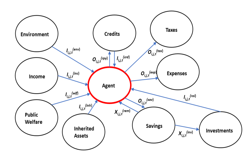
Fig. 1 shows the interaction of an agent with its economic environment. All incoming arrows are its available sources of wealth (inputs) and all outgoing ones are the areas where the wealth goes (outputs). An agent tries to maintain a balance among the inputs and outputs under changing scenarios (explained latter). Let there be $N$ agents in the system. These $N$ agents belong to $G$ income groups. $I_{i,j,t}^{(env)}$ denotes the input utility of $i^{th}$ agent from the $j^{th}$ income group derives from the environment at time $t$. $I_{i,j,t}^{(inc)}$ is the agent’s direct income, e.g., salary. $I_{i,j,t}^{(wlf)}$ is the public welfare it is entitled to. The agent inherits certain amount of wealth $I_{i,j,t}^{(inh)}$ from its legacy. The agent also gets a return on its investments amounting to $I_{i,j,t}^{(roi)}$. In case of need, it may borrow money from institutions in form of credits, insurances, etc., an amount of $I_{i,j,t}^{(crd)}$ and repays those credits, premiums, etc., which amount to $O_{i,j,t}^{(rpy)}$. The agent also pays direct tax of amount $O_{i,j,t}^{(tax)}$ on its income $I_{i,j,t}^{(inc)}$. Its expense (which may include indirect taxes) is $O_{i,j,t}^{(exp)}$. The agent also saves an amount of $O_{i,j,t}^{(sav)}$. In case of need, it also withdraws from this savings an amount of $X_{i,j,t}^{(rem)}$. It also invests an amount of $X_{i,j,t}^{(inv)}$ from its savings.

Income $I_{i,j,t}^{(inc)}$, is a uniform random value $X_{i,j,t}^{(inc)}$ between $I_{j}^{(min)}$ and $I_{j}^{(max)}$. Each income group $j$ has separate expense rate $\gamma_{j}$ and tax rate $\delta_{j}$. Public welfare $I_{i,j,t}^{(wlf)}$, is a uniform random value $X^{(wlf)}_{i,j,t}$ between $W_{j}^{(min)}$ and $W_{j}^{(max)}$. $I^{(inh)}_{i,j,0}$ is also initialised to a uniform random value between $V_{j}^{(min)}$ and $V_{j}^{(max)}$. The following sections describe changing scenarios an agent experiences along with the models for variation of the above parameters.

Figure 1. Economic interaction of an agent

3.1. Increase in expense over time

Expenses of agents can increase due to various reasons, such as, increased cost of living, inflation, etc. Increase in expense of $i^{th}$ agent over the time $t=1,2,..,T$ is defined by equation (1). Expense of each agent $i$ is assumed to increase linearly with time $t$.

(1) $$O^{(exp)}_{i,j,t}=[1+\alpha^{(exp)}_{i,j}t]\gamma_{j}I^{(inc)}_{i,j,t}$$

where $\alpha^{(exp)}_{i,j}$, $0<\alpha^{(exp)}_{i,j}\leq 1$, is used to control the increase over time.

3.2. Decrease in environment utility over time

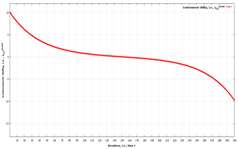
Each agent derives a certain utility from environment, such as, natural resources, suitable climatic conditions, etc. To model the varying environment utility, hyperbolic sine function, i.e., sinh(), is used. Hyperbolic sine function is used because environmental utility can be modeled from a situation when it provides the highest $A_{i,j}$ for the $i^{th}$ belonging to the $j^{th}$ group then progressively going down to zero and further declining (where degrading environment itself creates negative impact, e.g., extreme climatic conditions, natural disasters, etc.) to a minimum value of $-A_{i,j}$. Environment utility of $i^{th}$ agent belonging to the $j^{th}$ group at time $t$, $I^{(env)}_{i,j,t}$, varies as in equation (2) and it is normalized between $A_{i,j}$ and $-A_{i,j}$.

(2) $$I^{(env)}_{i,j,t}=[(A_{i,j}-(-A_{i,j})]\frac{\sinh(\alpha^{(env)}_{i,j}t-\frac{T}{2})-min{(\{\sinh(\alpha^{(env)}_{i,j}t-\frac{T}{2})\})}}{max{(\{\sinh(\alpha^{(env)}_{i,j}t-\frac{T}{2})\})}-min{(\{\sinh(\alpha^{(env)}_{i,j}t-\frac{T}{2})\})}}+(-A_{i,j})$$

$I^{(env)}_{i,j,t}$ is generated for the period $t=1,2,..,T$ and $\alpha^{(env)}_{i,j}$, $0<\alpha^{(env)}_{i,j}\leq 1$, is the control parameter.

3.3. Increase in taxes over time

Each income group has separate tax rate. Taxes is defined to increase linearly as shown in equation (3).

(3) $$O^{(tax)}_{i,j,t}=[1+\alpha^{(tax)}_{i,j}\frac{t}{T}]\delta_{j}I^{(inc)}_{i,j,t}$$

where $\delta_{j}$ is the tax rate for the $j^{th}$ income group. As before, $\alpha^{(tax)}_{i,j}$, $0<\alpha^{(tax)}_{i,j}\leq 1$, is used to adjust the rate of increase of taxes.

3.4. Decrease in public welfare over time

Each agent $i$ in income group $j$ has separate rate $\alpha^{(wlf)}_{i,j}$ to receive public welfare. Decreasing public welfare received by an agent is defined by equation (4).

(4) $$I^{(wlf)}_{i,j,t}=[1-\alpha^{(wlf)}_{i,j}\frac{t}{T}]X^{(wlf)}_{i,j,t},$$

where $0<\alpha^{(wlf)}_{i,j}\leq 1$ and $[1-\alpha^{(wlf)}_{i,j}\frac{t}{T}]>0$.

3.5. Decrease in income over time

Finally, income can decrease due to job losses and other factors which is defined by equation (5).

(5) $$I^{(inc)}_{i,j,t}=[1-\alpha^{(inc)}_{i,j}\frac{t}{T}]X^{(inc)}_{i,j,t}$$

where $\alpha^{(inc)}_{i,j}$, $0<\alpha^{(inc)}_{i,j}\leq 1$, is the control parameter and $[1-\alpha^{(inc)}_{i,j}\frac{t}{T}]>0$.

Thus, savings of agents after taxes and expenses is given by equation (6).

(6) $$O^{(sav)}_{i,j,t}=I^{(inc)}_{i,j,t}-O^{(tax)}_{i,j,t}-O^{(exp)}_{i,j,t}$$

If agent has a total accumulated credit of $I^{(crd)}_{i,j,t-1}$ at time $t-1$ and repays $\eta^{(rpy)}_{i}I^{(crd)}_{i,j,t-1}$ at time $t$ then credit repayment $O^{(rpy)}_{i,j,t}$ has to be subtracted from $O^{(sav)}_{i,j,t}$. Hence,

(7) $$O^{(rpy)}_{i,j,t}=\eta^{(rpy)}_{i}I^{(crd)}_{i,j,t-1}$$

(8) $$O^{(sav)}_{i,j,t}=O^{(sav)}_{i,j,t}-O^{(rpy)}_{i,j,t}$$

Maximum credit limit $I^{(crd)}_{i,j,0}$ is initialized to $\mu^{(crd)}_{i}I^{(inc)}_{i,j,0}$ at the beginning, i.e., at $t=0$.

(9) $$I^{(crd)}_{i,j,0}=\mu^{(crd)}_{i}I^{(inc)}_{i,j,0}$$

Investments is only possible if $O^{(sav)}_{i,j,t}>0$. If $\rho^{(inv)}_{i}$, $0<\rho^{(inv)}_{i}\leq 1$, is the rate from saving invested then this amount is given by

(10) $$X^{(inv)}_{i}=\rho^{(inv)}_{i}O^{(sav)}_{i,j,t}$$

and ROI is given by

(11) $$I^{(roi)}_{i,j,t}=I^{(roi)}_{i,j,t-1}+\rho^{(roi)}_{i}X^{(inv)}_{i}$$

where $\rho^{(roi)}_{i}$, $0<\rho^{(inv)}_{i}\leq 1$ is the rate of ROI. Remaining savings after investment of $i^{th}$ agent is given by

(12) $$X^{(rem)}_{i,j,t}=X^{(rem)}_{i,j,t-1}+[1-\rho^{(inv)}_{i}]O^{(sav)}_{i,j,t}$$

Net balance of $i^{th}$ agent is defined as

(13) $$X^{(net)}_{i,j,t}=X^{(net)}_{i,j,t-1}+I^{(env)}_{i,j,t}+I^{(wlf)}_{i,j,t}+I^{(roi)}_{i,j,t}+X^{(rem)}_{i,j,t}-abs[O^{(sav)}_{i,j,t}].$$

Absolute value of $O^{(sav)}_{i,j,t}$ is used to take care of it being negative when expenses and taxes together are more than the income.

3.6. Policy of agents

Algorithm 1 Balancing policy of agents

1:procedure AgentPolicy()

2:

3:       /* If net balance ¡ 0 then apply following policy */

4:       $If(X^{(net)}_{i,j,t}<0)$

5:             /* if agent has extra saving after then adjust from that amount */

6:             $If(X^{(rem)}_{i,j,t}>0)$

7:                   $deficit=abs(X^{(net)}_{i,j,t})$

8:                   $If(X^{(rem)}_{i,j,t}>deficit)$

9:                         $X^{(rem)}_{i,j,t}=X^{(rem)}_{i,j,t}-deficit$

10:                         $X^{(net)}_{i,j,t}=X^{(net)}_{i,j,t}+deficit$

11:                   $else$

12:                         $X^{(net)}_{i,j,t}=X^{(net)}_{i,j,t}+X^{(rem)}_{i,j,t}$

13:                          $X^{(rem)}_{i,j,t}=0$

14:                   $endif$

15:             $endif$

16:

17:             /* Still, if net balance ¡ 0 then adjust from ROI

18:             $If(X^{(net)}_{i,j,t}<0)$

19:                   $deficit=abs(X^{(net)}_{i,j,t})$

20:                   $If(I^{(roi)}_{i,j,t}>deficit)$

21:                         $I^{(roi)}_{i,j,t}=I^{(roi)}_{i,j,t}-deficit$

22:                         $X^{(net)}_{i,j,t}=X^{(net)}_{i,j,t}+deficit$

23:                   $else$

24:                         $X^{(net)}_{i,j,t}=X^{(net)}_{i,j,t}+I^{(roi)}_{i,j,t}$

25:                         $I^{(roi)}_{i,j,t}=0$

26:                   $endif$

27:             $endif$

28:

29:             /* Still, if net balance ¡ 0 then either adjust from credits or inherited assets */

30:             $If(X^{(net)}_{i,j,t}<0)$

31:                   /* Agent with index even prefers to avail credit */

32:                   $If(i\ is\ even)$

33:                         $deficit=abs(X^{(net)}_{i,j,t})$

34:                         $If(I^{(crd)}_{i,j,t}>deficit)$

35:                               $I^{(crd)}_{i,j,t}=I^{(crd)}_{i,j,t}-deficit$

36:                               $X^{(net)}_{i,j,t}=X^{(net)}_{i,j,t}+deficit$

37:                         $else$

38:                               $X^{(net)}_{i,j,t}=X^{(net)}_{i,j,t}+I^{(cred)}_{i,j,t}$

39:                               $I^{(crd)}_{i,j,t}=0$

40:                         $endif$

41:                   /* Agent with index odd prefers to avail inherited assets */

42:                   $else$

43:                         $deficit=abs(X^{(net)}_{i,j,t})$

44:                         $If(I^{(inh)}_{i,j,t}>deficit)$

45:                               $I^{(inh)}_{i,j,t}=I^{(inh)}_{i,j,t}-deficit$

46:                               $X^{(net)}_{i,j,t}=X^{(net)}_{i,j,t}+deficit$

47:                         $else$

48:                               $X^{(net)}_{i,j,t}=X^{(net)}_{i,j,t}+I^{(inh)}_{i,j,t}$

49:                               $I^{(inh)}_{i,j,t}=0$

50:                         $endif$

51:                   $endif$

52:             $endif$

53:       $endif$

54:end procedure

The agents apply the policies in Algorithm 1 when $X^{(net)}_{i,j,t}\geq 0$ to stabilize their economic conditions. As the first attempt, agents try to use their remaining savings $X^{(rem)}_{i,j,t}$ in lines 6-15. If $X^{(net)}_{i,j,t}<0$ still, then they try to use their ROI $I^{(roi)}_{i,j,t}$ in lines 18-27. Even then if $X^{(net)}_{i,j,t}<0$ then half of the agents (even ones) go for credit options in lines lines 32-40 and the remaining half (odd ones) use their inherited assets in lines 42-51. After applying these policies, agents with $X^{(net)}_{i,j,t}\geq 0$ are those who could balance inputs and outputs and stay afloat. Those agents who still have $X^{(net)}_{i,j,t}<0$ are designated as stress agents.

3.7. Matrices

The emergent behaviour of the following parameters over time are considered and studied in this paper.

3.7.1. Net Balance Amount

Net Balance Amount (NBA) at time $t$ is the sum of $X^{(net)}_{i,j,t}$ for all agents. Increase in this value means better economic condition and vice versa.

(14) $$NBA_{t}=\sum_{i=1}^{N}X^{(net)}_{i,j,t}$$

3.7.2. Remaining Saving Left

Remaining Saving Left (RSL) at time $t$ is the sum of $X^{(rem)}_{i,j,t}$ for all the agents. Increase in this value also means improved economic condition and vice versa.

(15) $$RSL_{t}=\sum_{i=1}^{N}X^{(rem)}_{i,j,t}$$

3.7.3. Number of Stressed Agents

Number of Stressed Agents (NSA) at time $t$ is the cardinality of the set of agents with $X^{(net)}_{i,j,t}<0$ after applying the policy algorithm. Increase in this value means higher economic distress.

(16) $$NSA_{t}=\|\{i:X^{(net)}_{i,j,t}<0\}\|$$

3.7.4. Return on Investment

Return on Investment (ROI) at time $t$ is the sum of $I^{(roi)}_{i,j,t}$ of all the agents. Increase in this value also means economic improvement and vice versa.

(17) $$ROI_{t}=\sum_{i=1}^{N}I^{(roi)}_{i,j,t}$$

3.7.5. Remaining Credit Limit

Remaining Credit Limit (RCL) at time $t$ is the sum of $I^{(crd)}_{i,j,t}$ for all the agents. Drop in this value means economic distress and vice versa.

(18) $$RCL_{t}=\sum_{i=1}^{N}I^{(crd)}_{i,j,t}$$

3.7.6. Remaining Inherited Assents

Remaining Inherited Assents (RIA) at time $t$ is the sum of $I^{(inh)}_{i,j,t}$ for all the agents. Decrease in this value also means economic distress.

(19) $$RIA_{t}=\sum_{i=1}^{N}I^{(inh)}_{i,j,t}$$

3.7.7. Total Stressed Credits

Total Stressed Credits (TSC) is difference between credits taken and amount repaid. If an agent has maximum credit limit $I^{(crd)}_{i,j,0}$ of 10 and has taken loan of 6, it has remaining credit $I^{(crd)}_{i,j,t}$ of 4. If it repays 2 then stressed credit is (6-2) = 4. Increase in this value also means deteriorating economic condition.

(20) $$TSC_{t}=\sum_{i=1}^{N}I^{(crd)}_{i,j,0}-I^{(crd)}_{i,j,t}-O^{(rpy)}_{i,j,t}$$

3.7.8. Savings after all Expenses

Savings after all Expenses (SAE) at time $t$ is the sum of $O^{(sav)}_{i,j,t}$ after paying taxes, expenses and credit repayment for all agents. Decrease in this value means deteriorating economic condition.

(21) $$SAE_{t}=\sum_{i=1}^{N}O^{(sav)}_{i,j,t}$$

3.7.9. Number of Stressed Agents in income group $j$

Number of Stressed Agents (NSA) in income group $j$ at time $t$ is the cardinality of the set of agents $X^{(net)}_{i,j,t}<0$. Increase in this value also means higher economic distress.

(22) $$NSA_{j,t}=\|\{i:X^{(net)}_{i,j,t}<0,j\in\{1,2,..,G\}\}\|$$

4. Results

This section presents the results from numerical evaluation of the model described above. Following scenarios are considered as explained above.

1. Impact of increase in expense of each agent

2. Impact of increase in expense and decrease in environment utility of each agent

3. Impact of increase in expense, decrease in environment utility and increase in taxation of each agent

4. Impact of increase in expense, decrease in environment utility, increase in taxation and decrease in welfare utility of each agent

5. Impact of increase in expense, decrease in environment utility, increase in taxation, decrease in welfare utility and decrease in income of each agent

In all the following results, the rules listed below hold good.

1. All the parameters are normalized to different ranges for better readability.

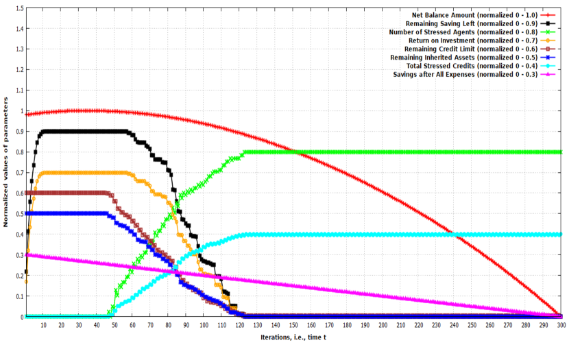
2. NBA, RSL , ROI, RCL, RIA, SAE, NSA and TSC are depicted with red, black, orange, brown, blue, pink, green and cyan lines respectively.

3. The normalization ranges of the above parameters are listed below.

   • NBA - (0.0 - 1.0)

   • RSL - (0.0 - 0.9)

   • NSA - (0.0 - 0.8)

   • ROI - (0.0 - 0.7)

   • RCL - (0.0 - 0.6)

   • RIA - (0.0 - 0.5)

   • TSC - (0.0 - 0.4)

   • SAE - (0.0 - 0.3)

4. The x-axis always represents the time steps, i.e., simulation iterations.

5. The y-axis always represents the normalized values of the parameters.

Values of the model parameters used for numerical evaluation are are presented in Table 1.

Table 1. Simulation Parameters

Parameter	Value	Description
$N$	100	Number of agents
$G$	3	Number of income groups: High $\rightarrow$ 10% of agents, Medium $\rightarrow$ 30% of agents and Low $\rightarrow$ 60% of agents
$\delta_{1},\delta_{2},\delta_{3}$	35%, 20%, 20%	Tax rates - High $\rightarrow$ 35%, Medium $\rightarrow$ 20%, Low $\rightarrow$ 10%
$\gamma_{1},\gamma_{2},\gamma_{3}$	25%, 40%, 98%	Expense rates - High $\rightarrow$ 25%, Medium $\rightarrow$ 40%, Low $\rightarrow$ 98%
$I_{1}^{(min)}$, $I_{2}^{(min)}$, $I_{3}^{(min)}$	8, 4, 1	Minimum income of three income groups
$I_{1}^{(max)}$, $I_{2}^{(max)}$, $I_{3}^{(max)}$	10, 7, 3	Maximum income of three income groups, Income of an agent is randomly chosen between these two min. and max. values
$V_{1}^{(min)}$, $V_{2}^{(min)}$, $V_{3}^{(min)}$	8, 4, 1	Minimum inherited assets of three income groups
$V_{1}^{(max)}$, $V_{2}^{(max)}$, $V_{3}^{(max)}$	10, 7, 3	Maximum inherited assets of three income groups. Inherited asset of an agent is randomly chosen between these two min. and max. values
$W_{1}^{(min)}$, $W_{2}^{(min)}$, $W_{3}^{(min)}$	1, 3, 5	Minimum welfare received by three income groups
$W_{1}^{(max)}$, $W_{2}^{(max)}$, $W_{3}^{(max)}$	2, 5, 7	Maximum welfare received by three income groups. Welfare received by an agent is randomly chosen between these two min. and max. values
$\mu^{(crd)}_{i}$	10	Assumed same for all agents
$\eta^{(rpy)}_{i}$	0.01	Assumed same for all agents
$\rho^{(inv)}_{i}$	0.50	Assumed same for all agents
$\rho^{(roi)}_{i}$	0.15	Assumed same for all agents
$\alpha^{(exp)}_{i,j}$	0.15	Assumed same for all agents
$\alpha^{(env)}_{i,j}$	0.025	Assumed same for all agents
$\alpha^{(tax)}_{i,j}$	1	Assumed same for all agents
$\alpha^{(inc)}_{i,j}$	1	Assumed same for all agents
$\alpha^{(wlf)}_{i,j}$	1	Assumed same for all agents
$T$	300	Simulation duration
$A_{i,j}$	10	Assumed same for all agents

4.1. Impact of Expense

Fig. 2 shows the impact of increase in expense on various parameters and their emergent behaviours. In each iteration, the expense of each agent is increased by 15% of its previous value, i.e., $\alpha^{(exp)}=0.15$. Even though the expenses increase, parameters RSL and ROI show improvements initial phase till iteration 10, i.e., $t=10$, and then stagnates, though SAE shows a downward trend continuously. NBA shows an increase till iteration $t=80$ and then starts declining with increased expenses. RIA and RCL still remains untouched, and NSA and TSC remain at their minimum values till $t=100$. However, there after the problem starts where agents start to meet their expenses through credits and RIA as both starts declining. A major deteriorating situation is observed around iterations $t=120$ where sharp decline in economic condition. Then, a short stable phase is observed. However, a complete collapse is observed round $t=150$. Thus, the model shows agents’ deteriorating condition with increased expenses. One key thing is that the transitions can be sharp (first one from 100 to 122 and the second one from 145 to 150) implying that there are thresholds when reached can cause major economic problems for the agents within a short time. Also, the transitions get sharper over time.

Figure 2. Emergent behaviour of various parameters with increase in expense

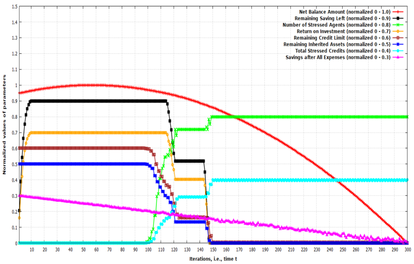
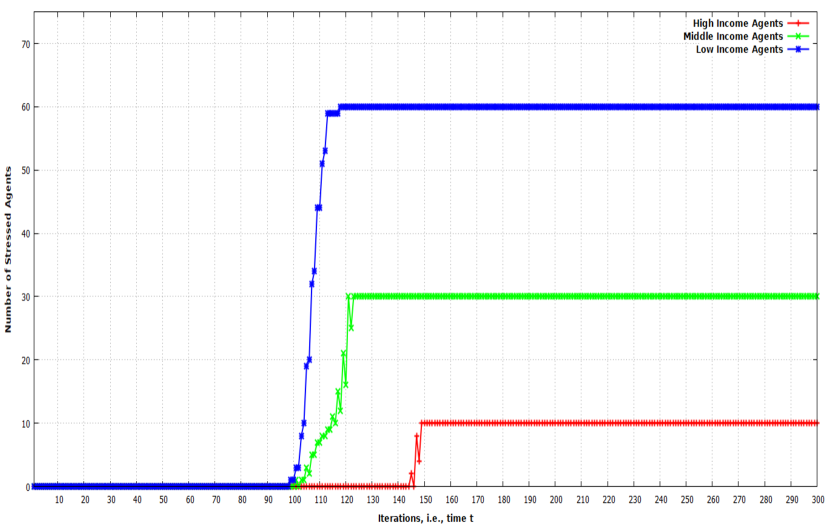
Fig. 3 shows the behaviour of stressed agents from three income groups with increase in expenses. It can be observed that as expense increases the number of stressed agents among the lower income group (blue line) gets impacted first and shows a sharp transition from minimum to maximum value from $t=98$ to $t=118$. The middle income group comes next with a longer phase transition from minimum to maximum from $t=100$ to $t=122$. The high income group is impacted last at a much later stage but still having a sharp transition from $t=145$ to $t=150$.

Figure 3. Number of stressed agents under three income categories with increase in expense

4.2. Impact of Expense and Environment

Fig. 4 shows the behaviour of environment utility, $I^{(env)}_{i,j,t}$ over time $t$. The values of $I^{(env)}_{i,j,t}$, $A_{i,j}$ and $\alpha^{(env)}_{i,j}$ are assumed same for all the agents to reduce complexity.

Figure 4. Environment utility vs. time

The emergent behaviour of various parameters with increase in expense and decrease in environment utility is plotted in Fig. 5. Though, the patterns are more or less similar to Fig. 2 the transitions in Fig. 5 occur much earlier between $t=67$ and $t=112$ as compared to the former. Also, the transitions are much more sharper compared to the previous case. The first transition occurs between $t=67$ and $t=90$ and the second one much sharper between $t=108$ and $t=112$.

Figure 5. Emergent behaviour of various parameters with increase in expense and decreasing environment utility

The behaviour of the stressed agents from the three income groups also show transitions much earlier compared to Fig. 3. The agents from lower income group shows sharper transition between $t=68$ and $t=78$ and those from other two groups remain the same between $t=68$ and $t=88$ and between $t=103$ and $t=108$ respectively.

Figure 6. Number of stressed agents under three income categories with increase in expense and decrease in environment utility

Thus, the model shows that increase in expense and decrease in environment utility lead to much higher economic distress compared to the former situation. The lower income group gets stressed much earlier.

4.3. Impact of Expense, Environment and Taxation

Fig. 7 shows the consequence of the different parameters when taxes increase along with increase in expense and decrease in environment utility for the agents. Though, the behaviour of the parameters remain the same as previous two scenarios, the transitions further shrinks in time, implying increased economic distress from $t=66$ to $t=89$ and then again $t=99$ from $t=105$.

Figure 7. Emergent behaviour of various parameters with increase in expense , decrease in environment utility and increase in taxes

The behaviour of the stressed agents of the three income groups shows faster transitions. Lower income groups shows a steeper curve from $t=65$ to $t=79$. Now, the middle income group also start showing steeper transitions between $t=70$ and $t=88$ as compared to the previous two cases. The high income group remains the same in its behaviour with transition between $t=100$ and $t=105$.

Figure 8. Number of stressed agents under three income categories with increase in expense, decrease in environment utility and increase in taxes

Thus, the model shows decrease in environment utility and increases in expenses and taxes lead to quicker degradation of economic conditions of agents.

4.4. Impact of Expense, Environment, Taxation and Welfare

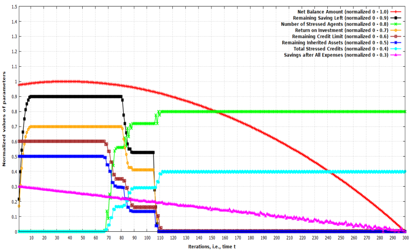
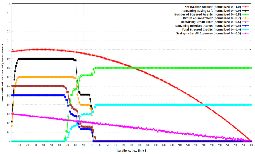
Fig. 9 shows the behaviour of all the parameters with increase in expense, decrease in environment utility, increase in tax and decrease in public welfare received. It can be observed that the transitions occur much quicker starting at $t=62$ till $t=84$ and collapsing at $t=99$ till $t=105$.

Figure 9. Emergent behaviour of various parameters with increase in expense, decrease in environment utility, increase in taxes and decrease in public welfare received

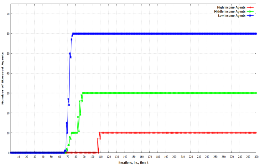
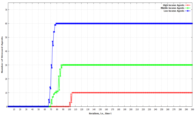
The stressed agents graph in Fig. 10 also shows further sharper transition compared to all the previous three situations. Low income group show increase from $t=63$ to $t=75$, middle income from $t=69$ to $t=87$ and high income from $t=99$ to $t=104$. Thus, this scenario leads to quicker deterioration of economic conditions of the agents.

Figure 10. Number of stressed agents under three income categories with increase in expense, decrease in environment utility and increase in taxes and decrease in public welfare utility

4.5. Impact of Expense, Environment, Taxation, Welfare and Income

Two scenarios are considered for reduced income of agents in addition to other factors in the previous scenarios. In the first case, agents reduce their expenses relative to their lower incomes. However in the second case, agents keep their expenses at their initial levels at $t=0$.

4.5.1. Expense is based on current income $I^{(inc)}_{i,j,t}$

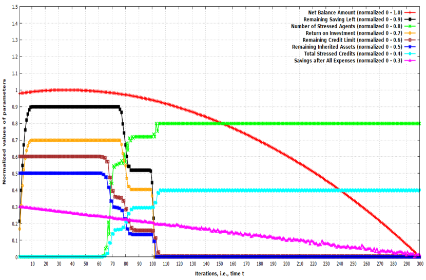
Fig. 11 shows the behaviour of parameters when increases in expense are fractions of present incomes of agents. Two things come into play in this scenario. Firstly, as income decreases the expenses of the agents also reduce. The increase in expense over time is relative to this reduced value. Secondly, when income decreases the direct taxes on income also comes down. It can be seen that the economic distress starts a bit late compared to the previous cases at $t=73$ and collapses completely at $t=137$ within a duration of 64. First transition happens between $t=73$ and $t=98$ and second one happens between $t=123$ and $t=137$. Also, SAEs increase due to decrease in taxes. However, these do not help stop the collapse due to other deteriorating factors.

Figure 11. Emergent behaviour of various parameters with increase in expense, decrease in environment utility, increase in taxes, decrease in public welfare received and decrease in income

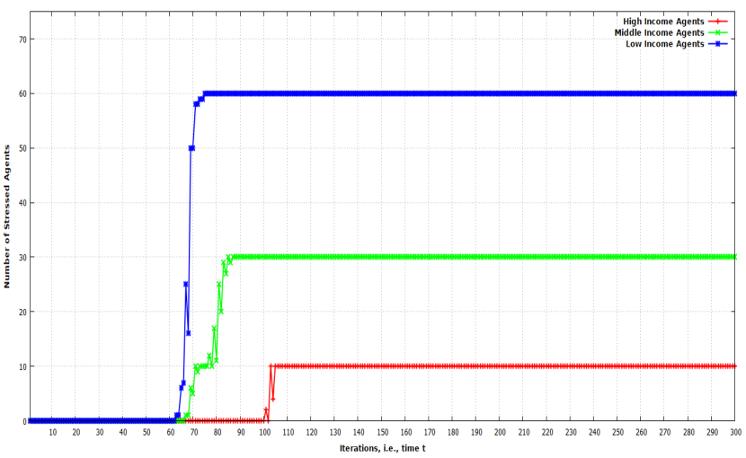
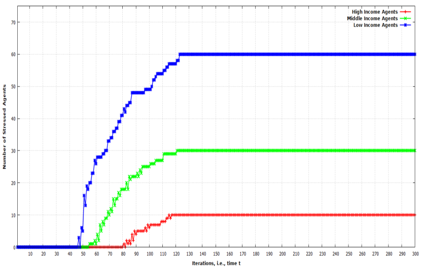
Low income groups deteriorates faster due to reduced income (Fig. 12). The middle and high income groups hold their ground for a longer duration before the final collapse.

Figure 12. Number of stressed agents under three income categories with increase in expense, decrease in environment utility and increase in taxes, decrease in public welfare received and decrease in income

4.5.2. Expense is based on $I^{(inc)}_{i,j,0}$

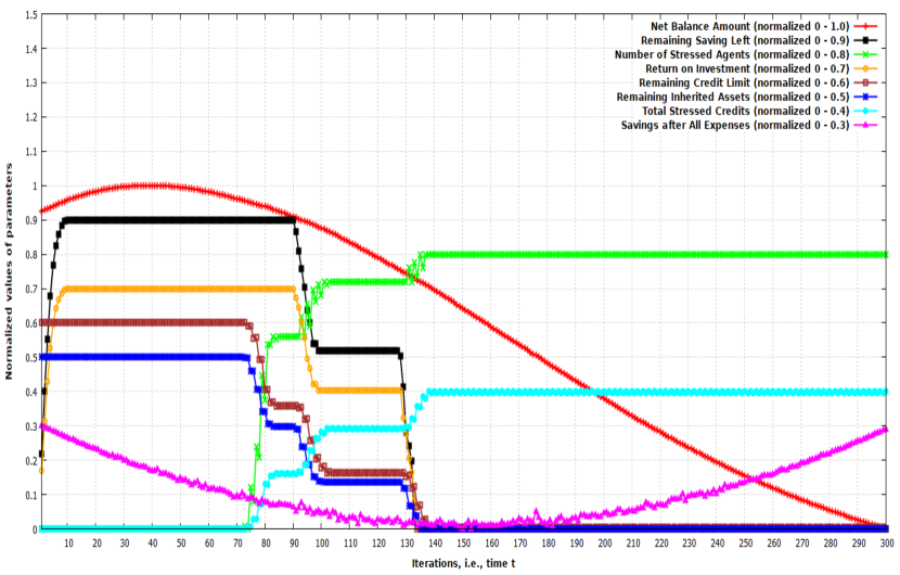
Fig. 13 shows the behaviour when expenses remain the same as at $t=0$ increase over time. Results show that the distresses start much early at $t=47$ and drag on till $t=123$ due to decreases in direct taxes. Surprisingly, there is only one declining trend unlike the previous cases where there is a stable phase between the two sharp transitions. Thus, decrease in income can bring distress much earlier with a continuous downward trend.

Figure 13. Emergent behaviour of various parameters with increase in (original) expense (fixed), decrease in environment utility, increase in taxes, decrease in public welfare received and decrease in income

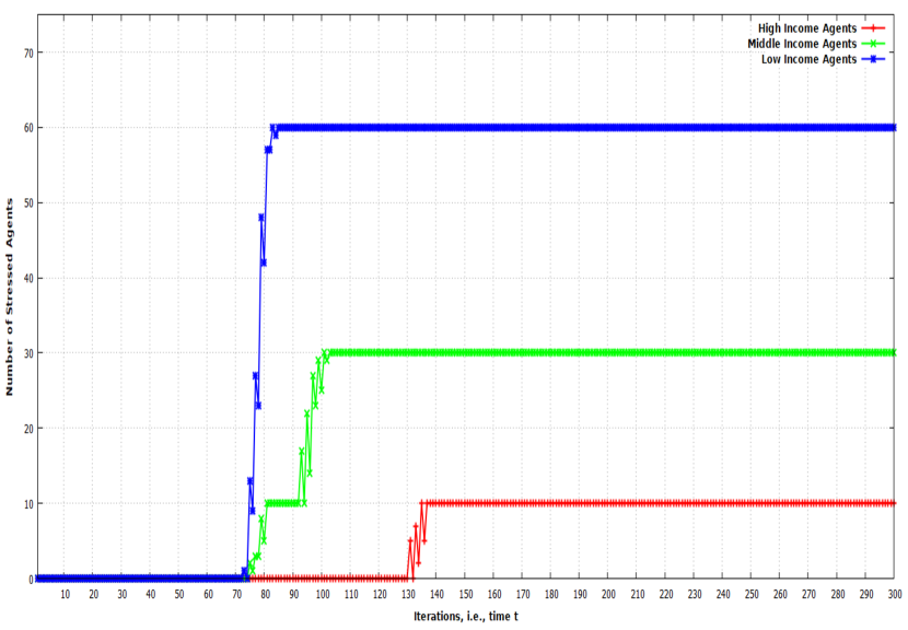
Another interesting fact is that the agents from all three income groups reach their peak values almost at the same time at $t=120$ (Fig. 14) even though distresses start much earlier at different times and are gradual compared to previous scenarios.

Figure 14. Number of stressed agents under three income categories with increase in expense, decrease in environment utility and increase in taxes, decrease in public welfare received and decrease in income

5. Discussion

Generally, following observations can be made of agents with progressively difficult economic conditions in the above five scenarios. Firstly, there are two transitions which are sharp implying that the economic collapse of agents can be sudden. Secondly, the second transition is sharper than the first which implies that the complete collapse can be faster. Thirdly, with increased economic burdens the transitions happen progressively faster and sharper, except for the case of decrease in income when it is delayed because of lower direct taxes to be paid by the agents. Fourthly, as expected, low income agents tend to collapse much faster, followed by the middle income group and finally the high income group. However, it is just a matter of time before all the agents are affected.

6. Conclusion

Post-pandemic world is seeing many challenges. These include high inflation, low growth, high debt, collapse of economies, political instability, job losses, lowering of income in addition to damages caused natural disasters and existing inequalities. Efforts are being made to mitigate these challenges at various levels. Research works have focussed on policies on specific scenarios, use cases, relationships between couple of sectors. However, understanding of actual impact of policies on individual agents and changing dynamics using a computational model has been largely unexplored. This paper explores progressive deteriorating conditions of increase in expense, degrading environmental utility, increase in taxation, decrease in welfare and lowering of income on agents with options to inherited properties, credits and return on investments using an agent based model. The paper also defines several parameters related to economic health of the group of agents in terms savings, ROI, credits, etc. Results indicate that collapse of agents’ economic condition can happen sharply for all income groups with increasing difficult conditions.

Future work will focus on more dynamic scenarios with different rate of change of parameters, such as, expense, income, tax, welfare, etc.

References

- (1)
- Bonam and Smădu (2021) Dennis Bonam and Andra Smădu. 2021. The long-run effects of pandemics on inflation: Will this time be different? Economics Letters 208 (2021), 110065. https://doi.org/10.1016/j.econlet.2021.110065
- Dang and Viet Nguyen (2021) Hai-Anh H. Dang and Cuong Viet Nguyen. 2021. Gender inequality during the COVID-19 pandemic: Income, expenditure, savings, and job loss. World Development 140 (2021), 105296. https://doi.org/10.1016/j.worlddev.2020.105296
- Otto and Gugushvili (2020) Adeline Otto and Dimitri Gugushvili. 2020. Eco-Social Divides in Europe: Public Attitudes towards Welfare and Climate Change Policies. Sustainability 12, 1 (2020). https://doi.org/10.3390/su12010404
- Lomborg (2020) Bjorn Lomborg. 2020. Welfare in the 21st century: Increasing development, reducing inequality, the impact of climate change, and the cost of climate policies. Technological Forecasting and Social Change 156 (2020), 119981. https://doi.org/10.1016/j.techfore.2020.119981
- Fleurbaey et al. (2018) Marc Fleurbaey, Maddalena Ferranna, Mark Budolfson, Francis Dennig, Kian Mintz-Woo, Robert Socolow, Dean Spears, and Stéphane Zuber. 2018. The Social Cost of Carbon: Valuing Inequality, Risk, and Population for Climate Policy. The Monist 102, 1 (12 2018), 84–109. https://doi.org/10.1093/monist/ony023 arXiv:https://academic.oup.com/monist/article-pdf/102/1/84/27215388/ony023.pdf
- Hirvilammi (2020) Tuuli Hirvilammi. 2020. The Virtuous Circle of Sustainable Welfare as a Transformative Policy Idea. Sustainability 12, 1 (2020). https://doi.org/10.3390/su12010391
- Fritz and Koch (2019) Martin Fritz and Max Koch. 2019. Public Support for Sustainable Welfare Compared: Links between Attitudes towards Climate and Welfare Policies. Sustainability 11, 15 (2019). https://doi.org/10.3390/su11154146
- Zachmann et al. (2018) Georg Zachmann, Gustav Fredriksson, and Grégory Claeys. 2018. The distributional effects of climate policies. Bruegel. Blueprint Series 28 (2018).
- Chateau et al. (2018) Jean Chateau, Ruben Bibas, and Elisa Lanzi. 2018. Impacts of Green Growth Policies on Labour Markets and Wage Income Distribution. 137 (2018). https://doi.org/https://doi.org/10.1787/ea3696f4-en
- Fujimori et al. (2018) Shinichiro Fujimori, Tomoko Hasegawa, Joeri Rogelj, Xuanming Su, Petr Havlik, Volker Krey, Kiyoshi Takahashi, and Keywan Riahi. 2018. Inclusive climate change mitigation and food security policy under 1.5C climate goal. Environmental Research Letters 13, 7 (jul 2018), 074033. https://doi.org/10.1088/1748-9326/aad0f7
- Conesa et al. (2020) Juan Carlos Conesa, Bo Li, and Qian Li. 2020. Welfare implications of switching to consumption taxation. Journal of Economic Dynamics and Control 120 (2020), 103991. https://doi.org/10.1016/j.jedc.2020.103991
- Koske et al. (2012) Isabell Koske, Jean-Marc Fournier, and Isabelle Wanner. 2012. Less Income Inequality and More Growth - Are They Compatible? Part 2. The Distribution of Labour Income. 925 (2012). https://doi.org/https://doi.org/10.1787/5k9h2975rhhf-en
- Mendenhall et al. (2012) Ruby Mendenhall, Kathryn Edin, Susan Crowley, Jennifer Sykes, Laura Tach, Katrin Kriz, and Jeffrey R. Kling. 2012. The Role of Earned Income Tax Credit in the Budgets of Low-Income Households. Social Service Review 86, 3 (2012), 367–400. https://doi.org/10.1086/667972 arXiv:https://doi.org/10.1086/667972
- Levi (2021) Sebastian Levi. 2021. Why hate carbon taxes? Machine learning evidence on the roles of personal responsibility, trust, revenue recycling, and other factors across 23 European countries. Energy Research & Social Science 73 (2021), 101883. https://doi.org/10.1016/j.erss.2020.101883
- Fremstad and Paul (2019) Anders Fremstad and Mark Paul. 2019. The Impact of a Carbon Tax on Inequality. Ecological Economics 163 (2019), 88–97. https://doi.org/10.1016/j.ecolecon.2019.04.016
- Pigato (2019) Miria A. Pigato (Ed.). 2019. Fiscal Policies for Development and Climate Action (1 ed.). https://www.worldbank.org/en/topic/macroeconomics/publication/fiscal-policies-for-development-and-climate-action
- Lamb et al. (2020) William F Lamb, Miklós Antal, Katharina Bohnenberger, Lina I Brand-Correa, Finn Müller-Hansen, Michael Jakob, Jan C Minx, Kilian Raiser, Laurence Williams, and Benjamin K Sovacool. 2020. What are the social outcomes of climate policies? A systematic map and review of the ex-post literature. Environmental Research Letters 15, 11 (nov 2020), 113006. https://doi.org/10.1088/1748-9326/abc11f
- Koch (2022) Max Koch. 2022. Social Policy Without Growth: Moving Towards Sustainable Welfare States. Social Policy and Society 21, 3 (2022), 447–459. https://doi.org/10.1017/S1474746421000361
- Tol (2019) Richard S.J. Tol. 2019. A social cost of carbon for (almost) every country. Energy Economics 83 (2019), 555–566. https://doi.org/10.1016/j.eneco.2019.07.006
- Catalano et al. (2020) Michele Catalano, Lorenzo Forni, and Emilia Pezzolla. 2020. Climate-change adaptation: The role of fiscal policy. Resource and Energy Economics 59 (2020), 101111. https://doi.org/10.1016/j.reseneeco.2019.07.005
- Bohnenberger (2020) Katharina Bohnenberger. 2020. Money, Vouchers, Public Infrastructures? A Framework for Sustainable Welfare Benefits. Sustainability 12, 2 (2020). https://doi.org/10.3390/su12020596
- Koval, Viktor et al. (2020) Koval, Viktor, Mikhno, Inesa, Trokhymets, Olena, Kustrich, Liliya, and Vdovenko, Nataliia. 2020. Modeling the interaction between environment and the economy considering the impact on ecosystem. E3S Web Conf. 166 (2020), 13002. https://doi.org/10.1051/e3sconf/202016613002
- Mikhno et al. (2021) Inessa Mikhno, Viktor Koval, Halyna Shvets, Oksana Garmatiuk, and Rima Tamosiuniene. 2021. Green Economy in Sustainable Development and Improvement of Resource Efficiency. Central European Business Review (oct 2021), 99–113. https://www.ceeol.com/search/article-detail?id=941002
- Carattini et al. (2021) Stefano Carattini, Garth Heutel, and Givi Melkadze. 2021. Climate Policy, Financial Frictions, and Transition Risk. Working Paper 28525. National Bureau of Economic Research. https://doi.org/10.3386/w28525
- Buchs et al. (2011) Milena Buchs, Nicholas Bardsley, and Sebastian Duwe. 2011. Who bears the brunt? Distributional effects of climate change mitigation policies. Critical Social Policy 31, 2 (2011), 285–307. https://doi.org/10.1177/0261018310396036 arXiv:https://doi.org/10.1177/0261018310396036
- Sivonen and Kukkonen (2021) Jukka Sivonen and Iida Kukkonen. 2021. Is There a Link between Welfare Regime and Attitudes toward Climate Policy Instruments? Sociological Perspectives 64, 6 (2021), 1145–1165. https://doi.org/10.1177/0731121421990053 arXiv:https://doi.org/10.1177/0731121421990053
- Joumard et al. (2012) Isabelle Joumard, Mauro Pisu, and Debbie Bloch. 2012. Tackling income inequality. (2012). https://doi.org/https://doi.org/10.1787/eco_studies-2012-5k95xd6l65lt
- Callan et al. (2013) Tim Callan, Brian Nolan, Claire Keane, Michael Savage, and John R. Walsh. 2013. Crisis, Response and Distributional Impact: The Case of Ireland. Papers WP456. Economic and Social Research Institute (ESRI). https://ideas.repec.org/p/esr/wpaper/wp456.html
- Marr et al. (2015) Chuck Marr, Chye-Ching Huang, Arloc Sherman, and Brandon DeBot. 2015. EITC and Child Tax Credit Promote Work, Reduce Poverty, and Support Children’s Development, Research Finds. (Oct. 2015). https://www.cbpp.org/research/federal-tax/eitc-and-child-tax-credit-promote-work-reduce-poverty-and-support-childrens
- MONTGOMERIE (2013) JOHNNA MONTGOMERIE. 2013. AMERICA’S DEBT SAFETY-NET. Public Administration 91, 4 (2013), 871–888. https://doi.org/10.1111/j.1467-9299.2012.02094.x arXiv:https://onlinelibrary.wiley.com/doi/pdf/10.1111/j.1467-9299.2012.02094.x
- Stiglitz (2019) Joseph E. Stiglitz. 2019. Addressing climate change through price and non-price interventions. European Economic Review 119 (2019), 594–612. https://doi.org/10.1016/j.euroecorev.2019.05.007
- Klenert et al. (2018) David Klenert, Linus Mattauch, Emmanuel Combet, Ottmar Edenhofer, Cameron Hepburn, Ryan Rafaty, and Nicholas Stern. 2018. Making carbon pricing work for citizens. Nature Climate Change 8, 8 (01 Aug 2018), 669–677. https://doi.org/10.1038/s41558-018-0201-2