Unsupervised Layer-wise Score Aggregation for Textual OOD Detection

Abstract

Out-of-distribution (OOD) detection for text applications is a rapidly growing field due to new robustness and security requirements driven by an increased number of AI-based systems. Existing OOD textual detectors often rely on an anomaly score (e.g., Mahalanobis distance) computed on the embedding output of the last layer of the encoder. In this work, we begin by uncovering that the fact that performance of existent methods varies greatly depending on the task and choice of the layer output. More importantly, we show that the usual choice (the last layer) is rarely the best one and thus, far better results could be achieved if the best layer were chosen. To leverage our key observation, we propose a data-driven, unsupervised method to combine layer-wise anomaly scores. In addition, we extend classical textual OOD benchmarks by including classification tasks with a greater number of classes (up to 77), which reflects more realistic settings. On this augmented benchmark, we show that the proposed post-aggregation methods achieve robust and consistent results while removing manual feature selection altogether. Their performance achieves near oracle’s best layer performance.

1 Introduction

With the increasing deployment of ML tools and systems, the issue of their safety and robustness is becoming more and more critical. Out-of-distribution robustness and detection have emerged as an important research direction Yang et al. (2021); Liu et al. (2020); Winkens et al. (2020a); Kirichenko et al. (2020); Liang et al. (2017); Vyas et al. (2018); Ren et al. (2019); Serrà et al. (2019); McAllister et al. (2019). These OOD samples can cause the deployed AI system to fail as neural models rely heavily on previously seen concepts or patterns Jakubovitz et al. (2019) and tend to struggle with anomalous samples Berend et al. (2020); Bulusu et al. (2020) or new concepts. These failures can affect user confidence, or even rule out the adoption of AI in critical applications. Distinguishing OOD samples (OUT) from in-distribution (IN) samples is a challenge when working on complex data structures (e.g., text or image) due to their high dimensionality. Although OOD detection has attracted much attention in computer vision Huang et al. ; Wang et al. ; Fang et al. (2022), few studies focused on textual data. Furthermore, distortion and perturbation methods for sensitivity analysis used in computer vision are not suitable due to the discrete nature of text Lee et al. (2022); Schwinn et al. (2021). A fruitful line of research Lee et al. (2018); Liang et al. (2018); Esmaeilpour et al. (2022); Xu et al. (2020); Huang et al. (2020) focuses on filtering methods to be added on top of pre-trained models without requiring retraining the model. These methods are often easy to deploy in a real-world scenario and thus lend themselves well to broad adoption. They include plug-in detectors that rely on softmax-based- or hidden-layer-based- confidence scores Lee et al. (2018); Liang et al. (2018); Esmaeilpour et al. (2022); Xu et al. (2020); Huang et al. (2020). Softmax-based detectors Liu et al. (2020); Pearce et al. (2021); Techapanurak et al. (2019) rely on the predicted probabilities to decide whether a sample is OOD. In contrast, hidden-layer-based scores (e.g., cosine similarity, data-depth Colombo et al. (2022a), or Mahalanobis distance Lee et al. (2018)) rely on input embedding of the model encoder. In natural language, these methods arbitrarily rely on either the embedding generated by the last layer of encoder Podolskiy et al. (2021) or on the logits Wang et al. (2022a); Khalid et al. (2022) to compute anomaly scores. While Softmax-based detectors can be applied in black-box scenarios, where one has only access to the model’s output, they have a very narrow view of the model’s behavior. In contrast, hidden-layer-based methods enable one to get deeper insights. They tend to yield better performance at the cost of memory and compute overhead.

We argue that the choice of the penultimate layers (i.e., the last layer, or the logits) ignores the multi-layer nature of the encoder and should be questioned. We give evidence that these representations are (i) not always the best choices (see Fig. 1) and (ii) that leveraging information from all layers can be beneficial. We introduce a data-driven procedure to exploit the information extracted from existing OOD scores across all the different layers of the encoder. While our method can be generalized to compute vision for visual transformers it appeared that in computer vision the last layer is more often than not the best layer to consider reducing the impact of aggregation or selection methods of the layers . We provide in App. H experiments in computer vision supporting these insights.

Our contribution can be summarized as follows:

1. We introduce a new paradigm. One of the main weaknesses of the previous methods is that they rely on a manual selection of the layer to be used, which ignores the information in the other layers of the encoder. We propose an automatic approach to aggregate information from all hidden layers without human (supervised) intervention. Our method, does not require access to OOD samples and harnesses information available in all layers by leveraging principled anomaly detection tools.

2. We conduct extensive experiments on our newly proposed benchmark: We introduce MILTOOD-C A MultI Lingual Text OOD detection benchmark for Classification tasks. MILTOOD-C alleviates two main limitations of previous works: (i) contrary to previous work that relies on datasets involving a limited number of classes (up to $5$), MILTOOD-C includes datasets with a higher number of classes (up to $77$ classes); (ii) MILTOOD-C goes beyond the English-centric setting and includes French, Spanish, and German datasets. Our experiments involve four models and over $186$ pairs of IN and OUT datasets, which show that our new aggregation procedures achieve high performance. At the same time, previous methods tend to suffer a drop in performance in these more realistic scenarios.

3. Open-Science & Open-source code. We will publish our code and benchmark in the datasets library Lhoest et al. (2021) to ensure reproducibility and reduce computational costs.

2 OOD detection for text classification

2.1 Background and notations

We adopt a text classification setting and rely on the encoder section of a model. Let $\Omega$ be a vocabulary and $\Omega^{*}$ its Kleene closure. We consider $(X,Y)$ a random variable with values in $\mathcal{X}\times\mathcal{Y}$ such that $\mathcal{X}\subseteq\Omega^{*}$ is the textual input space, and $P_{XY}$ is its joint probability distribution. The set $\mathcal{Y}=\left\{1,\ldots,C\right\}$ represents the classes of a classification task and $\mathcal{P}(\mathcal{Y})=\left\{\mathbf{p}\in[0,1]^{\left|\mathcal{Y}\right|}:\sum_{i=1}^{\left|\mathcal{Y}\right|}p_{i}=1\right\}$ the probability simplex over the classes. It is assumed that we have access to a training set $\mathcal{D}_{N}=\{(\mathbf{x}_{i},y_{i})\}_{i=1}^{N}$ composed of independent and identically distributed (i.i.d) realizations of $P_{XY}$. The Out-Of-Distribution (OOD) detection problem consists of deciding whether a new, previously unseen sample comes (or not) from the IN distribution $P_{XY}$. The goal is to build a binary function $g:\mathcal{X}\rightarrow\{0,1\}$ based on the thresholding of an anomaly score $s:\mathcal{X}\rightarrow\mathbb{R}_{+}$ that separates IN samples from OOD samples. Namely, for a threshold $\gamma\in\mathbb{R}_{+}$, we have: $g(\mathbf{x},\gamma)~{}=~{}\left\{\begin{array}[]{ll}1&\text{if }s\left(\mathbf{x}\right)>\gamma,\\ 0&\text{if }s\left(\mathbf{x}\right)\leqslant\gamma.\end{array}\right.$

2.2 Building an OOD detector

We assume that we have given a classifier $f_{\theta}:\mathcal{X}\rightarrow\mathcal{P}(\mathcal{Y})$ with $f_{\theta}=\operatorname{softmax}\circ~{}h\circ~{}f^{\theta}_{L}\circ f^{\theta}_{L-1}\circ\dots\circ f^{\theta}_{1}$, with $L>1$ layers (we omit the parameters $\theta$ in what follows for brevity’s sake.), where $f_{\ell}:\mathbb{R}^{d_{\ell-1}}\rightarrow\mathbb{R}^{d_{\ell}}$ is the $\ell$-th layer of the encoder with $d_{\ell}$ being the dimension of the latent space after the $\ell$-th layer ($d_{0}=d$). It is worth noting that in the case of transformers Vaswani et al. (2017), all latent spaces have the same dimension. Finally, $h$ represents the logit function of the classifier. To compute the anomaly score $s$ from $f_{\theta}$, OOD approaches rely on the hidden representations of the (multilayer) encoder. For $\mathbf{x}\in\mathcal{X}$ an input sequence, we denote $\mathbf{z}_{\ell}=(f_{\ell}\circ\dots\circ f_{1})(\mathbf{x})$ its latent representation at layer $\ell$. The latent representation obtained after the $\ell$-th layer of the training set is denoted as $\mathcal{D}_{N}^{\ell}=\{(\mathbf{z}_{\ell,i},y_{i})\}_{i=1}^{N}$. Furthermore, we denote by $\mathcal{D}_{N}^{\ell,y}$ the restriction of $\mathcal{D}_{N}^{\ell}$ to the samples with label $y$, i.e., $\mathcal{D}_{N}^{\ell,y}=\{(\mathbf{z}_{\ell,i},y_{i})\in\mathcal{D}^{\ell}_{N}:y_{i}=y\}$ with $N_{y}=|\mathcal{D}_{N}^{\ell,y}|$ indicates the cardinal of this set. Feature-based OOD detectors usually rely on three key elements:

1. Selecting features: the layer $\ell$ whose representation is considered to be the input of the anomaly score.

2. A notion of an anomaly (or novelty) score built on the mapping $\mathcal{D}_{N}^{\ell}$ of the training set on the chosen feature space. We can build such a score $s(\cdot,\mathcal{D}_{N}^{\ell})$ defined on $\mathbb{R}^{d}\times\left(\mathbb{R}^{d}\right)^{N}$ for any notion of abnormality.

3. Setting a threshold to build the final decision function.

Remark 1.

Choice of the threshold. To select $\gamma$, we follow previous work Colombo et al. (2022a) by selecting an amount of training samples (i.e., “outliers") the detector can wrongfully detect. A classical choice is to set this proportion to $80\%$.

2.3 Popular Anomaly Scores

Mahalanobis distance. Authors of Lee et al. (2018) (see also Podolskiy et al., 2021) propose to compute the Mahalanobis distance on the abstract representations of each layer and each class. Precisely, this distance is given by:

$$s_{M}(\mathbf{z}_{\ell},\mathcal{D}_{N}^{\ell,y})=\left(\mathbf{z}_{\ell}-\mu_{\ell,y}\right)^{\top}\Sigma_{\ell,y}^{-1}\left(\mathbf{z}_{\ell}-\mu_{\ell,y}\right)$$

on each layer $\ell$ and each class $y$ where $\mu_{\ell,y}$ and $\Sigma_{\ell,y}$ are the estimated class-conditional mean and covariance matrix computed on $\mathcal{D}_{N}^{\ell,y}$, respectively. The final score from Lee et al. (2018) is obtained by choosing the minimum of these scores over the classes on the penultimate encoder layer.

Integrated Rank-Weighted depth. Colombo et al. (2022a) propose to leverage the Integrated Rank-Weighted (IRW) depth (Ramsay et al., 2019; Staerman et al., 2021a). Similar to the Mahalanobis distance, the IRW data depth measures the centrality/distance of a point to a point cloud. For the $\ell$-th layer, a Monte-Carlo approximation of the IRW depth can be defined as:

$$s_{\text{IRW}}(\mathbf{z}_{\ell},\mathcal{D}_{N}^{\ell,y})=\frac{1}{n_{\mathrm{proj}}}\sum_{k=1}^{n_{\mathrm{proj}}}\min \Bigg{\{}\frac{1}{n}\sum_{i=1}^{N_{y}}\mathbbm{1}\left\{g_{k,i}(\mathbf{z}_{\ell})\leqslant 0\right\},\frac{1}{n}\sum_{i=1}^{N_{y}}\mathbbm{1}\left\{g_{k,i}(\mathbf{z}_{\ell})>0\right\}\Bigg{\}},$$

where $g_{k,i}(\mathbf{z}_{\ell})=\langle u_{k},\mathbf{z}_{\ell,i}-\mathbf{z}_{\ell}\rangle$, $u_{k}\in\mathbb{S}^{d-1},\mathbf{z}_{\ell,i}\in\mathcal{D}_{N}^{\ell,y}$ where $\mathbb{S}^{d-1}=\{x\in\mathbb{R}^{d}\;:\;||x||=1\}$ is the unit hypersphere and $n_{\mathrm{proj}}$ is the number of directions sampled on the sphere.

Cosine similarity. Zhou et al. (2021) propose to compute the maximum cosine similarity between the embedded sample $\mathbf{z}_{\ell}$ and the training set $\mathcal{D}_{N}^{\ell}$ at layer $\ell$:

$$s_{C}(\mathbf{z}_{\ell},\mathcal{D}_{N}^{\ell})=-\underset{\mathbf{z}_{\ell,i}\in\mathcal{D}_{N}^{\ell}}{\max}\;\;~{}\frac{\langle\mathbf{z}_{\ell},\mathbf{z}_{\ell,i}\rangle}{\left|\left|\mathbf{z}_{\ell}\right|\right|\left|\left|\mathbf{z}_{\ell,i}\right|\right|},$$

where $\langle\cdot,\cdot\rangle$ and $\left|\left|\cdot\right|\right|$ denote the Euclidean inner product and norm, respectively. They also choose the penultimate layer. It is worth noting they do not rely on a per-class decision.

2.4 Limitations of Existing Methods

The choice of layer for step (i) in Sec. 2.2 is not usually a question. Most work arbitrarily relies on the logits Liang et al. (2018); Liu et al. (2020) or the last layer of the encoder Winkens et al. (2020b); Podolskiy et al. (2021); Sun et al. (2022); Ren et al. (2019); Sastry & Oore (2020); Gomes et al. (2022); Yang et al. (2021); Hendrycks & Gimpel (2016); Wang et al. (2022a). We argue that these choices are unjustified and that previous work gives up on important information in other layers. Moreover, previous works have shown that all the layers carry different information or type of abstraction and thus are useful for different tasks Ilin et al. (2017); Kozma et al. (2018); Dara & Tumma (2018).

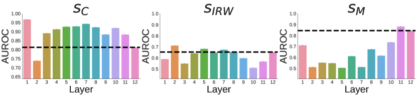
(a) Emotion

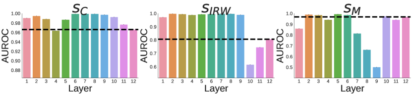
(b) 20-newsgroup

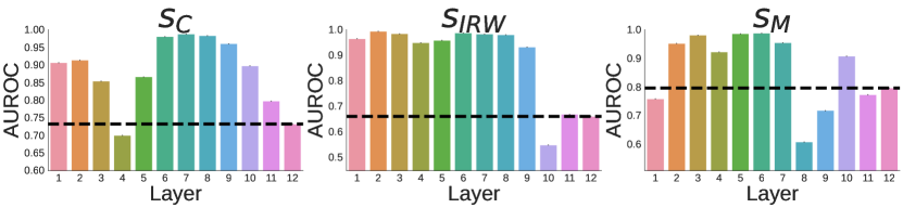
(c) IMDB

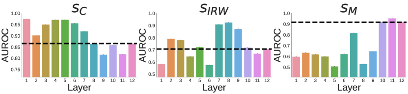
(d) Trec

Fig. 1: OOD detection performance in terms of AUROC $\uparrow$ for each features-based OOD score (Mahalanobis distance ($s_{M}$), Maximum cosine similarity ($s_{C}$) and IRW ($s_{IRW}$)) computed at each layer of the encoder for $4$ different OOD datasets (Emotion, 20-newsgroup, IMDB and Trec) for a model fine-tuned on SST2. We observe that the performance of each metric on each layer varies significantly with the OOD task.

To support our claim, we report in Fig. 1 the OOD performance of popular detectors described in Sec. 2.3 applied at each layer of the encoder Devlin et al. (2018). We observe a high variability across different layers. The last layer is rarely the best-performing layer, and there is room for improvement if we could choose the best possible layer or gather useful information from all of them. This observation is consistent with the literature, as neural networks are known to extract different information and construct different abstractions at each layer Ilin et al. (2017); Kozma et al. (2018); Dara & Tumma (2018). Only a few studies successfully address this issue and attempt to leverage information from all layers. Notably, recent work by Colombo et al. (2022a) considers representations obtained by taking the average embedding across the encoder layers. Other work Raghuram et al. (2021); Wang et al. (2022b) have been proposed in computer vision and adversarial attack settings but tend to fail in OOD detection settings. We propose to compute common OOD scores on each layer of the encoder (and not only on the logits or the representation generated by the last layer) and to aggregate this score in an unsupervised fashion to select and combine the most relevant following the task at hand.

3 Leveraging information from all layers

3.1 Problem Statement

For an input $\mathbf{x}\in\mathcal{X}$ and a training dataset $\mathcal{D}_{N}$, we obtain their set of embedding representation sets: $\{\mathbf{z}_{\ell}\}_{\ell=1}^{L}$ and $\{\mathcal{D}^{\ell}_{N}\}_{\ell=1}^{L}$, respectively. Given an anomaly score function $s:\;\mathbb{R}^{d}\times\left(\mathbb{R}^{d}\right)^{N}\rightarrow\mathbb{R}$ (e.g., those described in Sec. 2.3), we define the OOD score set of an input $\mathbf{x}$ as $\mathcal{S}_{s}(\mathbf{x};\mathcal{D}_{N})=\{\{s(\mathbf{z}_{\ell};\mathcal{D}^{\ell,y}_{N})\}_{\ell=1}^{L}\}_{y=1}^{C}\in\mathbb{R}^{L\times C}$. Similarly, it is possible to obtain a reference set of $\mathcal{R}(\mathcal{D}_{N})=\{\mathcal{S}_{s}(\mathbf{x};\mathcal{D}_{N}),\;\forall\;(\mathbf{x},y)\in\mathcal{D}_{N}\}$ from the training data. In what follows, we aim to answer: Can we leverage all the information available in $\mathcal{S}_{s}(\mathbf{x};\mathcal{D}_{N})$ and/or $\mathcal{R}(\mathcal{D}_{N})$ to build an OOD detector?

3.2 Proposed Framework

Our framework aims at comparing the set of scores of a sample to the sets of scores of a reference relying on principled anomaly detection algorithms. We propose a data-driven aggregation method of OOD scores, $\operatorname{Agg}$.

$$\operatorname{Agg}:\quad\mathbb{R}^{L\times C}\times\left(\mathbb{R}^{L\times C}\right)^{N} \rightarrow\mathbb{R}$$

$$(\mathcal{S}_{s}(\mathbf{x};\mathcal{D}_{N}),\mathcal{R}(\mathcal{D}_{N})) \rightarrow\operatorname{Agg}(\mathcal{S}_{s},\mathcal{R}),$$

where $\mathbf{x}$ denotes the input sample.

Intuition. This framework allows us to consider the whole trace of a sample through the model. This formulation has two main advantages: it avoids manual layer selection and enables us to leverage information from all the encoder layers.

We propose two families of approaches: (i) one solely relies on the score set $\mathcal{S}_{s}(\mathbf{x};\mathcal{D}_{N})$ (corresponding to a no-reference scenario and denoted as $\operatorname{Agg}_{\emptyset}$) and (ii) the second one (named reference scenario) leverages the reference set $\mathcal{R}(\mathcal{D}_{N})$.

Remark 2.

It is worth noting that our framework through $\operatorname{Agg}_{{\emptyset}set}$ or $\operatorname{Agg}$ naturally includes previous approaches Lee et al. (2018); Zhou et al. (2021); Colombo et al. (2022a). For example, the detector of Lee et al. (2018) can be obtained by defining $\operatorname{Agg}_{{\emptyset}}$ as the minimum of the penultimate line of the matrix $\mathcal{S}_{s}(\mathbf{x},\mathcal{D}_{N})$.

3.3 Detailed Aggregation Procedures

Fig. 2: Schema of our aggregation procedure. (1) We extract the embeddings at each layer of the encoder for every sample. (2) We compute the per-class scores for a reference set and the new sample to be evaluated for each layer embedding. (3) We aggregate the scores over every layer to get an aggregated per-class score before taking the min score over the classes. (4) Finally, we apply the threshold on this minimum.

Intuition. Our framework through $\operatorname{Agg}$ and $\operatorname{Agg}_{\emptyset}$ requires two types of operations to extract a single score from $\mathcal{S}_{s}(\mathbf{x},\mathcal{D}_{N})$ and $\mathcal{R}_{s}(\mathcal{D}_{N})$: one aggregation operation over the layers and one aggregation operation over the classes, where necessary.

Our framework in a nutshell. We assume we are given an anomaly score, $s$, that we want to enhance by leveraging all the layers of the encoder. For a given input $\mathbf{x}$, our framework follows $4$ steps (see Fig. 2 for a depiction of the procedure):

1. Compute the embeddings $\{\mathbf{z}_{l}\}_{l=1}^{L}$ for $\mathbf{x}$ and every element of $\mathcal{D}_{N}$.

2. Form $\mathcal{S}_{s}(\mathbf{x};\mathcal{D}_{N})$ and $\mathcal{R}(\mathcal{D}_{N})$ using the score $s$.

3. Perform $\operatorname{Agg}_{\emptyset}$ or $\operatorname{Agg}$:

   1. (per layer) Aggregate score information over the layers to obtain a vector composed of $C$ scores.

   2. (per class) Take the minimum value of this vector.

4. Apply a threshold $\gamma$ on that value.

Step (3.b). is inspired by the OOD literature (Lee et al., 2018; Colombo et al., 2022a). It relies on the observation that if the input sample is IN-distribution, it is expected to have at least one low score in the class vector, whereas an OOD sample should only have high scores equivalent to a high minimum score.

3.3.1 No-reference scenario ($\operatorname{Agg}_{\emptyset}$)

In the no-reference scenario, we have access to a limited amount of information. We thus propose to rely on simple statistics to aggregate the OOD scores available in $\mathcal{S}_{s}(\mathbf{x};\mathcal{D}_{N})$ to compute step (3). of the proposed procedure. Precisely, we use the average, the minimum (min), the median (med), and coordinate (see Remark 2) operators on the column of the matrix $\mathcal{S}_{s}(\mathbf{x};\mathcal{D}_{N})$.

3.3.2 Data-driven scenario ($\operatorname{Agg}$)

In the data-driven scenario, $\operatorname{Agg}$ also has access to the set of reference OOD scores (i.e., $\mathcal{R}_{s}(\mathcal{D}_{N})$) for the given OOD score $s$. The goal, then, is to compare the score set $\mathcal{S}_{s}(\mathbf{x};\mathcal{D}_{N})$ of the input with this reference set $\mathcal{R}_{s}(\mathcal{D}_{N})$ to obtain a score vector of size $C$. In the following, we propose an original solution for the layer operation.

For the per layer operation we rely on an anomaly detection algorithm for each class $\mathcal{A}_{y}$ defined as:

$$\mathcal{A}_{y}:\mathbb{R}^{L}\times(\mathbb{R}^{L})^{N_{y}} \rightarrow\mathbb{R}$$

$$\mathbf{s}_{y}\times\mathcal{R}_{y} \mapsto\mathcal{A}_{y}(\mathbf{s}_{y},\mathcal{R}_{y}),$$ (1)

where $\mathbf{s}_{y}=\{s(\mathbf{z}_{\ell};\mathcal{D}^{\ell,y}_{N})\}_{\ell=1}^{L}$ and $\mathcal{R}_{y}=\mathcal{R}(\mathcal{D}_{N}^{y})$.

Remark 3.

$\mathcal{A}_{y}$ is trained on the reference set $\mathcal{R}_{y}$ for each class and thus does not involve any OOD samples. The score returned for a vector $\mathbf{s}_{y}$ is the prediction score associated with the trained algorithm.

Remark 4.

We define a per-class decision for $\operatorname{Agg}$ since it has been shown to be significantly more effective than global scores Huang & Li (2021). It is the approach chosen by most state-of-the-art-methods. We have validated this approach by conducting extensive experiments. We refer the reader to App. C for further discussion.

We propose four popular anomaly detection algorithms. First, we propose to reuse common OOD scores ($s_{M}$, $s_{C}$, $s_{\text{IRW}}$) as aggregation methods(See App. C for more details): they are now trained on the reference set of sets of OOD scores $\mathcal{R}_{s}(\mathcal{D}_{N})$ and provide a notion of anomaly for the trace of a sample through the model. In addition, we used Isolation Forest (IF; Liu et al., 2008, see also Hariri et al., 2019; Staerman et al., 2019 for its extensions), see also Amer et al., 2013) and the Local Outlier Factor (LOF; Breunig et al., 2000). Below, we briefly recall the general insights of each of these algorithms. It is important to emphasize that our framework can accommodate any anomaly detection algorithms (further details are given in App. C).

Local Outlier Factor. This method compares a sample’s density with its neighbors’ density. Any sample with a lower density than its neighbors is regarded as an outlier.

Isolation Forest. This popular algorithm is built on the idea that anomalous instances should be easily distinguished from normal instances. It leads to a score that measures the complexity of separating a sample from others based on the number of necessary decision trees required to isolate a data point. It is computationally efficient, benefits from stable hyper-parameters, and is well suited to the unsupervised setting.

3.4 Comparison to Baseline Methods

Current State-of-the-art methods for OOD detection on textual data have been recently provided in Colombo et al. (2022a) (PW). They aggregate the hidden layers using Power means Hardy et al. (1952); Rücklé et al. (2018) and then apply an OOD score on this aggregated representation. They achieved previous SOTA performance by coupling it with the IRW depth and proposed a comparison with Mahalanobis and Cosine versions. We reproduce these results as it is a natural baseline for aggregation algorithms.

Last Layer. Considering that the model’s last layer or logits should output the most abstract representation of an input, it has been the primary focus of attention for OOD detection. It is a natural choice for any architecture or model and therefore removes the hurdle of selecting features for different tasks and architectures. For this heuristic, we obtain OOD scores using the Mahanalobis distance (as in Lee et al., 2018), the IRW score (as in Colombo et al., 2022a), and the cosine similarity (as in Winkens et al., 2020b).

Additional methods. It is common on OOD detection methods to report the Maximum Softmax Prediction (MSP; Hendrycks & Gimpel, 2016) as well as the Energy Score (E; Liu et al., 2020).

4 MILTOOD-C: A more realistic benchmark for OOD detection

4.1 Limitation of Existing Benchmarks

Number of classes. Text classification benchmarks for OOD detection often consist of sentiment analysis tasks involving a small number of classes Fang & Zhan (2015); Kharde et al. (2016). Those tasks with a larger number of classes have been mostly ignored in previous OOD detection benchmarks Colombo et al. (2022a); Li et al. (2021); Zhou et al. (2021). However, real-world problems do involve vastly multi-class classification tasks Casanueva et al. (2020). Previous work in computer vision found that these problems require newer and carefully tuned methods to enable OOD detection in this more realistic setting Deng et al. (2009); Le & Yang (2015).

Monolingual datasets. Most methods have been tested on architectures tailored for the English language Colombo et al. (2022a); Li et al. (2021); Arora et al. (2021). With inclusivity and diversity in mind Ruder (2022); van Esch et al. (2022), it is necessary to assess the performance of old and new OOD detection methods on a variety of languages Srinivasan et al. (2021); de Vries et al. (2020); Baheti et al. (2021); Zhang et al. (2022).

4.2 Benchmark

We now present MILTOOD-C, which addresses the aforementioned limitations. It consists of more than $25$ datasets involving up to $77$ classes, and $4$ languages.

Dataset selection. We gathered a large and diverse benchmark in terms of shift typology, tasks, and languages. It covers $25$ datasets in $4$ different languages (i.e., English, German, Spanish, and French) and classifications tasks involving $2$ to $77$ classes. Following standard protocol Hendrycks et al. (2020), we train a classifier for each in-distribution dataset (IN-DS) while the OOD dataset (OUT-DS) is coming from a different dataset. We provide a comprehensive list of the $180$ pairs we considered in Sec. A.2. It is an order of magnitude larger than recent concurrent work from Colombo et al. (2022a).

English benchmark. We relied on the benchmark proposed by Zhou et al. (2021); Hendrycks et al. (2020). It features three types of IN-DS: sentiment analysis (i.e., SST2 Socher et al. (2013), IMDB Maas et al. (2011)), topic classification (i.e., 20Newsgroup Joachims (1996)) and question answering (i.e., TREC-10 and TREC-50 Li & Roth (2002)). We also included the Massive FitzGerald et al. (2022) dataset and the Banking Casanueva et al. (2020) for a larger number of classes and NLI datasets (i.e., RTE Burger & Ferro (2005); Hickl et al. (2006) and MNLI Williams et al. (2018)) following Colombo et al. (2022a). We also considered HINT3Arora et al. (2020) and clink clink which feature a large number of classes. We form IN and OOD pairs between the aforementioned tasks.

Beyond English-centric tasks. For language-specific datasets, we added the same tasks as for English when available and extended it with language-specific datasets such as the PAWS-S datasets Yang et al. (2019), film reviews in French and Spanish Blard (2019). For French and German, we also added the Swiss judgments datasets Niklaus et al. (2022). Finally, we added different tweet classification tasks for each language (English, German, Spanish and French) Zotova et al. (2020); Barbieri et al. (2022).

Model selection. To ensure that our results are consistent not only across tasks and shifts, but also across model architectures, we train classifiers based on $6$ different Transformer Vaswani et al. (2017) decoders: BERT Devlin et al. (2018) (base, large and multilingual versions), DISTILBERT Sanh et al. (2019) and RoBERTa Liu et al. (2019) (base and large versions) fine-tuned on each task.

4.3 Assessing OOD detection performance

	$\mathcal{A}$	AUROC $\uparrow$		FPR $\downarrow$		Err
$\operatorname{Agg}$	$s_{M}$	0.88	±0.16	0.32	±0.35	0.16	±0.19
	$s_{C}$	0.91	±0.16	0.21	±0.35	0.13	±0.21
	$s_{IRW}$	0.87	±0.18	0.30	±0.39	0.16	±0.21
	IF	0.92	±0.13	0.21	±0.31	0.10	±0.15
	LOF	0.87	±0.15	0.37	±0.36	0.19	±0.22
$\operatorname{Agg}_{\emptyset}$	Mean	0.84	±0.18	0.43	±0.40	0.24	±0.25
	Median	0.83	±0.17	0.46	±0.39	0.25	±0.25
	PW	0.82	±0.17	0.48	±0.39	0.23	±0.23
Bas.	$E$	0.83	±0.18	0.39	±0.30	0.19	±0.18
	Last layer	0.84	±0.17	0.42	±0.37	0.20	±0.22
	Logits	0.75	±0.16	0.60	±0.34	0.30	±0.25
	MSP	0.83	±0.17	0.39	±0.28	0.19	±0.18

Tab. 1: Overall average performance of each aggregation method for all architectures, tasks, and OOD scores.

OOD detection is a binary classification problem where the positive class is OUT. We evaluate our detectors following concurrent work Colombo et al. (2022a); Darrin et al. (2022) and evaluate our them using threshold-free metrics such as AUROC $\uparrow$, AUPR-IN/AUPR-OUT and threshold based metrics such as FPR $\downarrow$ at $95\%$ and Err. We report detailed definitions of the metrics in Sec. A.3.

5 Experimental Results

5.1 Quantifying Aggregation Gains

Overall results. Data driven aggregation methods (i.e., with reference) consistently outperform any other baselines or tested methods by a significant margin (see Tab. 1 and Tab. 2) on our extensive MILTOOD-C benchmark. According to our experiments, the best combination of hidden feature-based OOD score and aggregation function is to use the Maximum cosine similarity as the underlying OOD score and to aggregate these scores using the IRW data depth ($s_{\text{IRW}}$). A first time to get the abnormality of the representations of the input and a second time to assess the abnormality of the set of layer-wise scores through the model. It reaches an average AUROC $\uparrow$ of $0.99$ and a FPR $\downarrow$ of $0.02$. It is a gain of more than $5\%$ compared to the previous state-of-the-art methods.

		$\mathcal{A}$	AUROC $\uparrow$	FPR $\downarrow$	Err
$s_{M}$	$\operatorname{Agg}$	$s_{M}$	0.90 ±0.14	0.27 ±0.33	0.16 ±0.20
		$s_{C}$	0.88 ±0.17	0.32 ±0.40	0.19 ±0.24
		$s_{IRW}$	0.81 ±0.20	0.44 ±0.42	0.23 ±0.23
		IF	0.94 ±0.10	0.19 ±0.25	0.11 ±0.13
		LOF	0.87 ±0.15	0.39 ±0.37	0.22 ±0.25
	$\operatorname{Agg}_{\emptyset}$	Mean	0.74 ±0.18	0.59 ±0.39	0.32 ±0.27
		Median	0.75 ±0.17	0.61 ±0.35	0.33 ±0.25
		PW	0.80 ±0.17	0.61 ±0.38	0.30 ±0.25
	Bas.	Last layer	0.92 ±0.11	0.25 ±0.31	0.13 ±0.17
		Logits	0.71 ±0.14	0.65 ±0.27	0.33 ±0.23
$s_{C}$	$\operatorname{Agg}$	$s_{M}$	0.93 ±0.11	0.20 ±0.27	0.11 ±0.15
		$s_{C}$	0.98 ±0.10	0.04 ±0.19	0.03 ±0.11
		$s_{IRW}$	0.99 ±0.07	0.02 ±0.15	0.02 ±0.08
		IF	0.94 ±0.14	0.12 ±0.29	0.04 ±0.12
		LOF	0.93 ±0.11	0.20 ±0.26	0.11 ±0.14
	$\operatorname{Agg}_{\emptyset}$	Mean	0.93 ±0.12	0.25 ±0.33	0.16 ±0.21
		Median	0.92 ±0.12	0.27 ±0.34	0.17 ±0.23
		PW	0.93 ±0.11	0.19 ±0.27	0.11 ±0.14
	Bas.	Last layer	0.92 ±0.11	0.22 ±0.26	0.11 ±0.13
		Logits	0.81 ±0.17	0.52 ±0.42	0.28 ±0.29
$s_{\text{IRW}}$	$\operatorname{Agg}$	$s_{M}$	0.81 ±0.18	0.50 ±0.38	0.21 ±0.21
		$s_{C}$	0.89 ±0.17	0.28 ±0.36	0.17 ±0.21
		$s_{IRW}$	0.82 ±0.19	0.43 ±0.39	0.24 ±0.21
		IF	0.89 ±0.15	0.34 ±0.36	0.17 ±0.19
		LOF	0.82 ±0.15	0.54 ±0.35	0.27 ±0.24
	$\operatorname{Agg}_{\emptyset}$	Mean	0.84 ±0.18	0.47 ±0.40	0.24 ±0.24
		Median	0.82 ±0.18	0.50 ±0.39	0.26 ±0.24
		PW	0.74 ±0.17	0.64 ±0.34	0.31 ±0.24
	Bas.	Last layer	0.66 ±0.14	0.79 ±0.21	0.38 ±0.23
		Logits	0.73 ±0.16	0.64 ±0.28	0.29 ±0.20
MSP	Bas.	MSP	0.83 ±0.17	0.39 ±0.28	0.20 ±0.18

Tab. 2: Average performance of each considered metric over all the OOD pairs and model architectures in terms of AUROC $\uparrow$, Err, and FPR $\downarrow$ . For each common OOD score, we report the results obtained using every aggregation method or choice of features to consider.

Most versatile aggregation method. While the $s_{C}$ and $s_{\text{IRW}}$ used as aggregation methods achieve excellent performance when paired with $s_{C}$ as the underlying OOD score, they fail to aggregate as well other underlying scores. Whereas the isolation forest algorithm is a more versatile and consistent data-driven aggregation method: it yields performance gain for every underlying OOD score.

Performance of common baselines. We show that, on average, using the last layer or the logits as features to perform OOD detection leads to poorer results than almost every other method. It is interesting to point out that this is not the case in computer vision Yang et al. (2021). This finding further motivates the development of OOD detection methods tailored for text.

Impact of simple statistical aggregation. Interestingly, simple statistical aggregations of the set of OOD scores, such as the average or the median, achieve, in some cases, similar or even better results than baselines relying on the score of a single layer.

Impact of data-driven aggregation. In most scenarios, aggregating the scores using a data-driven anomaly detection method leads to significant gains in performance compared to baseline methods. This supports the idea that useful information is scattered across the layers. We show that this information can be retrieved and effectively leveraged to improve OOD detection.

5.2 Post Aggregation Is More Stable Across Task, Language, Model Architecture

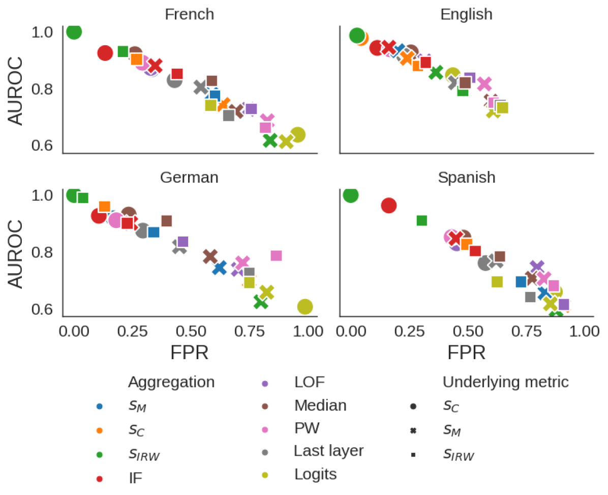
(a) Comparison of the best-performing aggregation methods and underlying OOD scores in terms of AUROC $\uparrow$ and FPR $\downarrow$ trade-off. We can see that most OOD detectors’ performance varies greatly from language to language. The maximum cosine similarity scores aggregated with IRW (green circle) can maintain its performance in all four studied languages and the isolation forests.

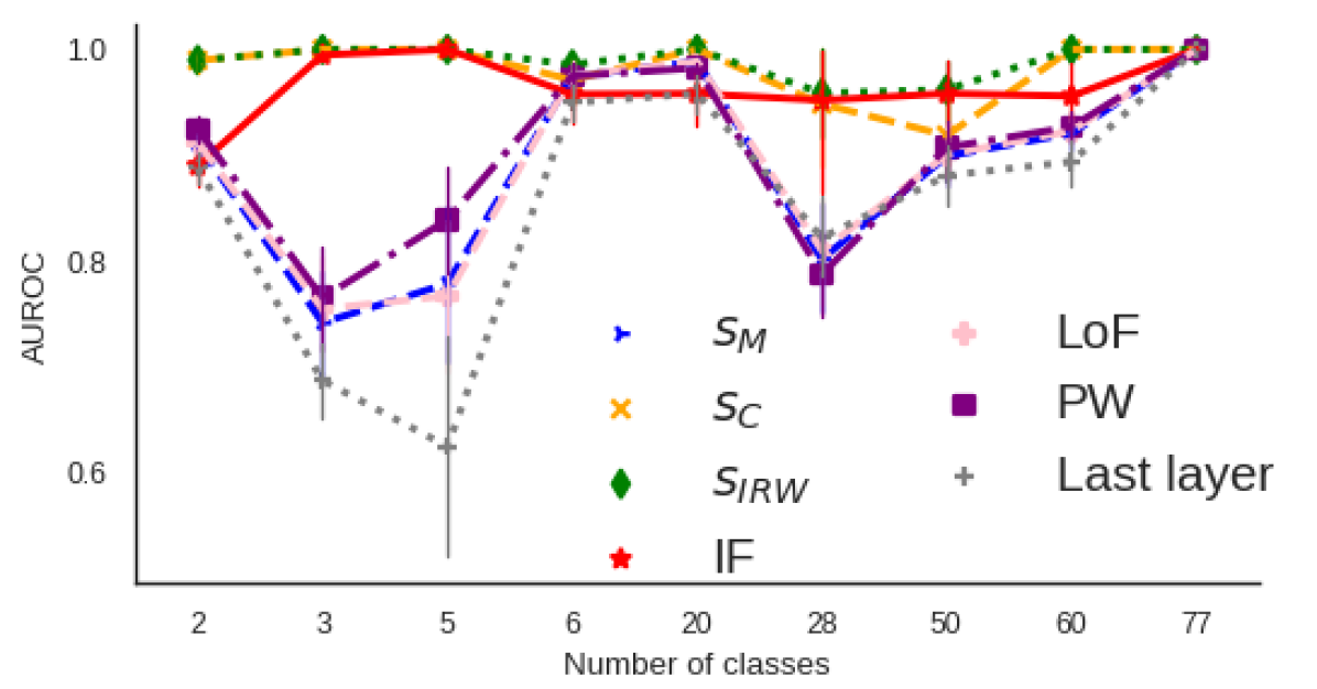
(b) Average performance of OOD detectors in terms of AUROC $\uparrow$ for tasks involving different numbers of classes.

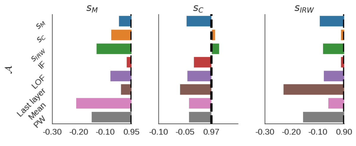
(c) Average performance difference in terms of AUROC between aggregation methods and the oracle (best possible layer).

Fig. 3: Performance trade-off, behavior on tasks featuring different number of classes and comparison with oracle performance.

Most OOD scores have been crafted and finetuned for specific settings. In the case of NLP, they have usually been validated only on datasets involving a small number of classes or on English tasks. In this section, we study the stability and consistency of the performance of each score and aggregation method in different settings.

Stability of performance across tasks. In 3(b), we plot the average AUROC $\uparrow$ across our models and datasets per number of classes of the IN dataset. It is, therefore, the number of classes output by the model. Our best post-aggregation methods (i.e., Maximum cosine similarity and Integrated Rank-Weigthed) produced more consistent results across all settings. It can maintain excellent performance for all types of datasets, whereas the performance of baselines and other aggregation methods tends to fluctuate from one setting to another. More generally, we observe that data-driven aggregation methods tend to perform consistently on all tasks, whereas previous baselines’ performance tends to vary.

Stability of results across languages. In 3(a), we show the relation between AUROC $\uparrow$ and FPR $\downarrow$ for all our aggregation methods and underlying metrics for each language we studied. In contrast, the performance of most combinations varies with the language. We especially notice that $s_{C}$ scores aggregated using either the Integrated rank-weighted or $s_{C}$ consistently achieve excellent performance across all languages.

6 Limitations and conclusions

While this method yields good performance for filtering OOD data and thus allows the exclusion of samples that would undoubtedly be mishandled by the model, it can’t provide any solid guarantees or certification. Moreover, it focused on filtering samples that seemed different from the training distribution without regard for the actual performance of the model on these samples. It might very well exclude samples that would have been well processed on the basis that they are too different from the training distribution. We believe though that it can be a valuable tool to enable a safer deployment of language models in production by allowing efficient filtering of (supposedly) unsupported inputs. We proposed a new framework that allows aggregating OOD scores across all the layers of the encoder of a text classifier instead of solely relying on scores computed on the logits or output of the last layer to improve OOD detection. We confirmed that all the layers of the encoder of a text classifier are not equal when it comes to OOD detection and, more importantly, that the common choices for OOD detection (logits and last layer) are, more often than not, not the best choice. We validated our methods on an extended text OOD classification benchmark MILTOOD-C that we introduced. We showed that our aggregation methods are not only able to outperform previous baselines and recent work, but they were also able to outperform an oracle that would be able to choose the best layer to perform OOD detection for a given task. This leads us to conclude that there is useful information for OOD detection scattered across all the layers of the encoder of a text classifier and that, when appropriately extracted, it can be leveraged to improve OOD detection performance vastly.

[sections]

[sections]l1

Appendix A Benchmark details

A.1 Datasets references

Tab. 3: List of Datasets

Dataset Name	URL
SetFit/emotion	https://huggingface.co/datasets/SetFit/emotion
banking77 Casanueva et al. (2020)	https://huggingface.co/datasets/banking77
SetFit/20-newsgroupsLang (1995)	https://huggingface.co/datasets/SetFit/20_newsgroups
imdb Maas et al. (2011)	https://huggingface.co/datasets/imdb
AmazonScience/massive FitzGerald et al. (2022)	https://huggingface.co/datasets/AmazonScience/massive
glue Wang et al. (2018)	https://huggingface.co/datasets/glue
super-glue Wang et al. (2019)	https://huggingface.co/datasets/super_glue
sst2 Socher et al. (2013)	https://huggingface.co/datasets/sst2
trec Hovy et al. (2001)	https://huggingface.co/datasets/trec
go-emotions Demszky et al. (2020)	https://huggingface.co/datasets/go_emotions
clinc-oos Larson et al. (2019)	https://huggingface.co/datasets/clinc_oos
HINT3 Arora et al. (2020)	https://github.com/hellohaptik/HINT3
xquad Artetxe et al. (2019)	https://huggingface.co/datasets/xquad
catalonia-independence	https://huggingface.co/datasets/catalonia_independence
muchocine	https://huggingface.co/datasets/muchocine
allocine Blard (2019)	https://huggingface.co/datasets/allocine
paws-x Yang et al. (2019)	https://huggingface.co/datasets/paws-x
swiss-judgment-prediction Niklaus et al. (2022)	https://huggingface.co/datasets/rcds/swiss_judgment_prediction
xnli Conneau et al. (2018)	https://huggingface.co/datasets/xnli/
tweet-sentiment-multilingual Barbieri et al. (2022)	https://huggingface.co/datasets/cardiffnlp/tweet_sentiment_multilingual
xstanceVamvas & Sennrich (2020)	https://huggingface.co/datasets/x_stance

A.2 OOD pairs

		OUT-DS
Language	IN-DS
English	20ng	go-emotions,sst2,imdb,trec,mnli,snli,rte,b77,massive,trec-fine,emotion
	b77	go-emotions,sst2,imdb,20ng,trec,mnli,snli,rte,massive,trec-fine,emotion
	emotion	go-emotions,sst2,imdb,20ng,trec,mnli,snli,rte,b77,massive,trec-fine
	go-emotions	sst2,imdb,20ng,trec,mnli,snli,rte,b77,massive,trec-fine,emotion
	imdb	go-emotions,sst2,20ng,trec,mnli,snli,rte,b77,massive,trec-fine,emotion
	massive	go-emotions,sst2,imdb,20ng,trec,mnli,snli,rte,b77,trec-fine,emotion
	rte	go-emotions,sst2,imdb,20ng,trec,mnli,snli,b77,massive,trec-fine,emotion
	sst2	go-emotions,imdb,20ng,trec,mnli,snli,rte,b77,massive,trec-fine,emotion
	trec	go-emotions,sst2,imdb,20ng,mnli,snli,rte,b77,massive,trec-fine,emotion
	trec-fine	go-emotions,sst2,imdb,20ng,trec,mnli,snli,rte,b77,massive,emotion
French	fr-allocine	fr-cls,fr-xnli,fr-pawsx,fr-xstance,fr-swiss-judgement,fr-tweet-sentiment
	fr-cls	fr-xnli,fr-pawsx,fr-allocine,fr-xstance,fr-swiss-judgement,fr-tweet-sentiment
	fr-pawsx	fr-cls,fr-xnli,fr-allocine,fr-xstance,fr-swiss-judgement,fr-tweet-sentiment
	fr-swiss-judgement	fr-cls,fr-xnli,fr-pawsx,fr-allocine,fr-xstance,fr-tweet-sentiment
	fr-tweet-sentiment	fr-cls,fr-xnli,fr-pawsx,fr-allocine,fr-xstance,fr-swiss-judgement
	fr-xnli	fr-cls,fr-pawsx,fr-allocine,fr-xstance,fr-swiss-judgement,fr-tweet-sentiment
	fr-xstance	fr-cls,fr-xnli,fr-pawsx,fr-allocine,fr-swiss-judgement,fr-tweet-sentiment
German	de-pawsx	de-xstance,de-swiss-judgement,de-tweet-sentiment
	de-swiss-judgement	de-xstance,de-tweet-sentiment,de-pawsx
	de-tweet-sentiment	de-xstance,de-swiss-judgement,de-pawsx
	de-xstance	de-swiss-judgement,de-tweet-sentiment,de-pawsx
Spanish	es-cine	es-tweet-sentiment,es-pawsx,es-tweet-inde
	es-pawsx	es-tweet-sentiment,es-cine,es-tweet-inde
	es-tweet-inde	es-tweet-sentiment,es-pawsx,es-cine
	es-tweet-sentiment	es-pawsx,es-cine,es-tweet-inde

Tab. 4: List of OOD pairs considered in our benchmark for each language., the name reported here in this table are the names of the datasets on the Huggingface datasets hub.

	Dataset	Number of classes
Language
English	go-emotions	28
	sst2	2
	imdb	2
	20ng	20
	b77	77
	massive	60
	trec-fine	50
	emotion	6
	trec	6
	rte	2
	mnli	3
	snli	3
French	cls	2
	xnli	3
	pawsx	2
	allocine	2
	xstance	2
	swiss-judgement	2
	tweet-sentiment	3
German	xstance	2
	swiss-judgement	2
	tweet-sentiment	3
	pawsx	2
Spanish	tweet-sentiment	3
	pawsx	2
	cine	5
	tweet-inde	3

Tab. 5: Details of the datasets composing MILTOOD-C.

A.3 OOD detection performance metrics

For evaluation we follow previous work in anomaly detection Picot et al. (2023b, a); Guerreiro et al. (2023); Gomes et al. and use AUROC $\uparrow$, FPR $\downarrow$ , AUPR-IN/AUPR-OUT and Err. We do not aggregate the scores using mean aggregation accross metrics Colombo (2021a); Colombo et al. (2022b).

Area Under the Receiver Operating Characteristic curve (AUROC $\uparrow$; Bradley, 1997). The Receiver Operating Characteristic curve is curve obtained by plotting the True positive rate against the False positive rate. The area under this curve is the probability that an in-distribution example $\mathbf{X}_{in}$ has a anomaly score higher than an OOD sample $\mathbf{x}_{out}$: AUROC $\uparrow$$=\Pr(s(\mathbf{x}_{in})>s(\mathbf{x}_{out}))$. It is given by $\gamma\mapsto(\Pr\big{(}s(\mathbf{x})>\gamma\,|\,Z=0\big{)},\Pr\big{(}s(\mathbf{x})>\gamma\,|\,Z=1\big{)})$.

False Positive Rate at $95\%$ True Positive Rate (FPR $\downarrow$ ). We accept to allow only a given false positive rate $r$ corresponding to a defined level of safety and we want to know what share of positive samples we actually catch under this constraint. It leads to select a threshold $\gamma_{r}$ such that the corresponding TPR equals $r$. At this threshold, one then computes: $\Pr(s(\mathbf{x})>\gamma_{r}\,|\,Z=0)$ with $\gamma_{r}$ s.t. $\textrm{TPR}(\gamma_{r})=r$. $r$ is chosen depending on the difficulty of the task at hand and the required level of safety.

Area Under the Precision-Recall curve (AUPR-IN/AUPR-OUT; Davis & Goadrich, 2006). The Precision-Recall curve plots the recall (true detection rate) against the precision (actual proportion of OOD amongst the predicted OOD). The area under this curve captures the trade-off between precision and recall made by the model. A high value represents a high precision and a high recall i.e. the detector captures most of the positive samples while having few false positives.

Detection error (Err). It is simply the probability of miss-classification for the best threshold.

Appendix B Layer importance in OOD detection

Our extensive experiments consistently show that there almost always exists a layer that is excellent at separating OOD data.

		AUROC $\uparrow$
Ours	Aggregation
$\operatorname{Agg}$	$s_{M}$	0.88	±0.16
	$s_{C}$	0.91	±0.16
	$s_{IRW}$	0.85	±0.19
	IF	0.92	±0.13
	LOF	0.87	±0.15
$\operatorname{Agg}_{\emptyset}$	Mean	0.84	±0.18
	PW	0.82	±0.17
Oracle	Oracle	0.94	±0.12

Tab. 6: Average performance of aggregation scores along with the performance of the oracle that is able to select the best layer to perform OOD detection.

In Tab. 7 we present the AUROC $\uparrow$ performance of all aggregation with all metrics in comparison with the oracle’s performance. We see that there is much room for improvement and that we are able to extract these improvements and even go further.

			AUROC $\uparrow$
Metric	Ours	Aggregation
$s_{M}$	$\operatorname{Agg}$	$s_{IRW}$	0.82	±0.20
		LOF	0.87	±0.15
		$s_{C}$	0.88	±0.17
		$s_{M}$	0.91	±0.14
		IF	0.94	±0.10
	$\operatorname{Agg}_{\emptyset}$	Mean	0.74	±0.18
		PW	0.80	±0.17
	Oracle	Oracle	0.95	±0.09
$s_{C}$	$\operatorname{Agg}$	$s_{M}$	0.93	±0.11
		LOF	0.93	±0.11
		IF	0.94	±0.14
		$s_{C}$	0.98	±0.09
		$s_{IRW}$	0.99	±0.07
	$\operatorname{Agg}_{\emptyset}$	PW	0.93	±0.11
		Mean	0.93	±0.11
	Oracle	Oracle	0.97	±0.07
$s_{IRW}$	$\operatorname{Agg}$	$s_{M}$	0.81	±0.18
		$s_{IRW}$	0.81	±0.19
		LOF	0.82	±0.15
		$s_{C}$	0.88	±0.18
		IF	0.89	±0.15
	$\operatorname{Agg}_{\emptyset}$	PW	0.74	±0.17
		Mean	0.84	±0.18
	Oracle	Oracle	0.90	±0.16

Tab. 7: Performance per metrics and aggregation with the oracle aggregation for comparison

B.1 Explainability and layer significance

Best Layer Selection (Oracle). In Fig. 1, we showed that high OOD detection performance could be reached, provided that we know which is the best layer to perform the OOD detection on. We compare our aggregation methods to an oracle method that always uses the best layer. We show in 3(c) that our aggregation’s methods outperform baselines and, in some cases, the performance of the oracle. This means that our aggregation methods reach and even outperform oracle performance.

Retro-engineering and explainability. We propose an explainability analysis of the learned aggregation algorithms to gain more insights into the layer selection retained by our data-driven detectors. We report in Fig. 4 the SHAP scores Lundberg & Lee (2017) of one of them to distinguish Go-Emotions samples from RTE samples and 20 news-group samples. It outlines the different importance of the layers for different tasks. Not surprisingly, we found that different layers better separate different classes and tasks. We also confirm that the last layer is not always the best suited for OOD data separation.

Fig. 4: Importance (in terms of Shap score Lundberg & Lee, 2017) of each layer in OOD detection for Go-Emotions as IN-DS with BERT for two different OOD datasets. It represents the importance of each feature (Mahalanobis distance computed at a given layer) for the isolation forest anomaly detection algorithms. We can see that the significant layers are different from one OOD dataset to another and that in both presented cases, the last layer ($12$) nor the logits ($13$) are not the most useful ones.

Appendix C Additional aggregation algorithms

We proposed in our work a framework that accommodates a wide range of aggregation algorithms. We focused on unsupervised anomaly detection algorithms and common statistics. However, many others options are available in different flavors. For instance, we focused on per-class anomaly detection but we can redo all our work for all classes at once or implement common OOD scores as aggregation mechanisms. In this section, we propose additional aggregation algorithms that are worth exploring. We provide their formalization and results when available and propose direction for future works.

C.1 Details of anomaly detection algorithms

Local Outlier Factor It measures the density of objects around a sample to decide whether it is an inlier or an outlier. It relies on the $k$-distance of a sample, e.g, its distance to its $k$th closest neighbor and considers $N_{k}(\mathbf{x})$ the set of the $k$ nearest neighbors.

For stability reasons, the usual LOF method uses the reachability distance which is defined as $\operatorname{Rd}(\mathbf{x},\mathbf{x}^{\prime})=\max(k-\operatorname{distance}(\mathbf{x}^{\prime}),d(\mathbf{x},\mathbf{x}^{\prime}))$. Intuitively, it is the distance between $\mathbf{x}$ and $\mathbf{x}^{\prime}$ if they are far enough from each other otherwise they are in the same $k$ nearest neighbors set and in that case the diameter of the set is used as minimal distance. From these definitions, we can define the local density of a sample $\mathbf{x}$, $\operatorname{dens}(\mathbf{x})=\left(\frac{\sum_{\mathbf{x}^{\prime}\in N_{k}(\mathbf{x})}\operatorname{Rd}_{k}(\mathbf{x},\mathbf{x}^{\prime})}{\left|N_{k}(\mathbf{x})\right|}\right)$. The LOF score compare the density of a sample to the densities of its neighbor: $\texttt{LOF}(\mathbf{x})=\frac{\sum_{\mathbf{x}^{\prime}\in N_{k}(\mathbf{x})}\operatorname{dens}_{k}(\mathbf{x}^{\prime})}{\left|N_{k}(\mathbf{x})\right|\operatorname{dens}_{k}(\mathbf{x})}$. If $\texttt{LOF}(\mathbf{x})=1$ the sample has the same density as his neighbor, if it’s lower than $1$ it has a higher density than its neighbor and thus is likely to be an inlier whereas if the score is higher than $1$ it has a smaller density than its neighbor and should be an outlier.

Isolation Forest This popular algorithm is built on the idea that abnormal instances should be easier to distinguish from normal instances. It leads to a score that measures the complexity of separating samples based on the number of necessary decision trees required to isolate a data point. In addition to its computational ease, it benefits from stable hyper-parameters and is well suited to the unsupervised setting. Formally speaking we consider a recursive partitioning problem which is formalized as an isolation tree structure. The number of trees required to isolate a point is the length of a path through the tree from the root to a leaf.

C.2 Per-class scoring vs. Global aggregation

We reproduced the common strategy of relying on a per-class OOD score and then using the minimum score over the classes as the OOD score. This strategy relies on the intuition that an IN sample, belonging to a given class will at least have a small anomaly score regarding this class whereas an OOD sample would have only high scores.

However, using our aggregation tools we can imagine relying on per-class OOD scores for the underlying scores but including them in the aggregation mechanism. For comprehensiveness’ sake, we report here the results under this setting but we found that in most cases per-class scores remain the better solution.

Following our notations and framework, it means formally that the aggregation algorithms are now not indexed by the classes but take as input a vector containing all the scores per layer and per class:

$$\mathcal{A}: (\mathcal{R}^{L}\times\mathcal{R}^{C})\times(\mathcal{R}^{L}\times\mathcal{R}^{C})^{N}\rightarrow\mathbb{R}$$

$$\mathbf{s}\times\mathcal{R}\mapsto\mathcal{A}(\mathbf{s},\mathcal{R}),$$ (2)

		AUROC $\uparrow$		FPR $\downarrow$		Err
Ours	Aggregation
$\operatorname{Agg}$	$s_{C}*$	0.55	±0.09	0.92	±0.14	0.48	±0.27
	$s_{M}*$	0.81	±0.18	0.45	±0.40	0.22	±0.23
	$s_{IRW}*$	0.79	±0.19	0.55	±0.39	0.29	±0.26
	IF*	0.83	±0.16	0.36	±0.32	0.22	±0.22
	LoF*	0.50	±0.00	1.00	±0.02	0.45	±0.30

Tab. 8: Overall average performance of each aggregation method overall architectures, tasks and underlying OOD scores when aggregating all layers and classes at once.

			AUROC $\uparrow$		FPR $\downarrow$		Err
Metric	Ours	Aggregation
$s_{M}$	$\operatorname{Agg}$	$s_{C}*$	0.57	±0.12	0.89	±0.19	0.48	±0.27
		$s_{M}*$	0.75	±0.16	0.67	±0.35	0.33	±0.25
		$s_{IRW}*$	0.67	±0.14	0.77	±0.27	0.38	±0.23
		IF*	0.75	±0.15	0.55	±0.29	0.34	±0.21
		LoF*	0.50	±0.01	0.99	±0.03	0.42	±0.28
$s_{C}$	$\operatorname{Agg}$	$s_{C}*$	0.51	±0.01	0.97	±0.02	0.50	±0.27
		$s_{M}*$	0.75	±0.16	0.53	±0.34	0.28	±0.21
		$s_{IRW}*$	0.82	±0.19	0.47	±0.38	0.24	±0.24
		IF*	0.84	±0.15	0.34	±0.32	0.23	±0.24
		LoF*	0.50	±0.00	1.00	±0.00	0.44	±0.29
$s_{\text{IRW}}$	$\operatorname{Agg}$	$s_{C}*$	0.58	±0.10	0.91	±0.14	0.45	±0.26
		$s_{M}*$	0.93	±0.15	0.16	±0.31	0.07	±0.11
		$s_{IRW}*$	0.86	±0.18	0.43	±0.40	0.26	±0.29
		IF*	0.91	±0.13	0.19	±0.25	0.11	±0.15
		LoF*	0.50	±0.00	1.00	±0.00	0.50	±0.30

Tab. 9: Average performance of the aggregation methods (i.e., for $\operatorname{Agg}$) performed on the whole score matrix at once (per-class and per-layer scores concatenated into a single vector) instead of aggregation each trajectory separately.

Overall aggregation vs per-class aggregation. Consistently with previous work, our aggregation methods do not perform as well when used to produce directly a single overall score instead of being used class-wise and then taking the minimum score over the classes. In Tab. 9 we report the OOD detection performance of this setting.

C.3 Without reference statistical baselines

The simplest way to aggregate OOD scores is to consider statistical aggregation over the layers and the classes. We showed that even basic aggregations such as taking the median score enable significant gains with respect to the last layer baselines.

Appendix D Computational cost

Time complexity. While the addition of an aggregation method induces obvious additional computational costs they are actually quite limited (they do not slow down the process significantly. They require only to compute the usual OOD scores on each layer (which does not change the asymptotic complexity) and then to perform the inference of common anomaly detection algorithms. For example, Isolation forests are known to have a linear complexity in the number of samples and to be able to perform well and fast with numerous and very high dimensional data.

Memory footprint. Perhaps most of the overhead is a memory overhead: for underlying OOD scores relying on a reference set we have to store one trained score for each layer. In the case of the Mahalanobis distance, it means storing $L$ covariance matrices instead of one in addition of the trained aggregation algorithm.

Appendix E Explainability and variability

Isolation forests are constructed by choosing at random separating plans and thus each run might give different importance to features. We benchmarked the methods over $10$ seeds to alleviate variability and validate our results. It showed that while some features could be permuted the overall trend were consistent: features that are not relevant for a run do not significantly gain in importance.

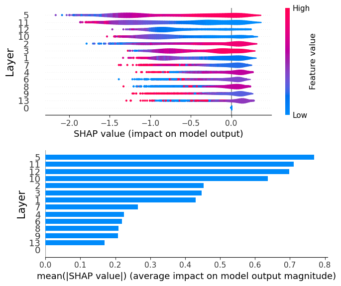
(a) RTE as Out-DS

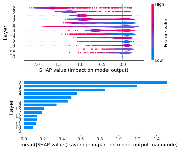
(b) 20ng as Out-DS

Fig. 5: Importance (in terms of shap score Lundberg & Lee (2017)) of each layer in OOD detection for Go-Emotions as IN-DS with a bert architecture for two different OOD datasets. The first row represents the samples from a dataset containing IN and OUT samples. Each line corresponds to a feature and shows how a given feature’s value influences the model to rule the sample as an anomaly (negative) or as a normal (positive) sample. The features are ranked by importance in the decision. The second row represents the importance of each feature (OOD score computed at a given layer) for the isolation forest anomaly detection algorithms. We can see that the significant layers are different from one OOD dataset to another and that in both presented cases, the last layer (Layer 12) is not the most useful one.

Appendix F Experimental results

F.1 Performance per tasks

F.1.1 Language specific results

In Tab. 10, Tab. 11, Tab. 13, Tab. 12 we present the average performance of each aggregation methods on each language.

			AUROC $\uparrow$		FPR $\downarrow$		Err		AUPR-IN		AUPR-OUT
Metric	Ours	Agg.
$E$	Bas.	$E$	0.86	±0.16	0.35	±0.29	0.17	±0.17	0.82	±0.25	0.81	±0.22
$s_{M}$	Bas.	Last layer	0.92	±0.11	0.24	±0.30	0.12	±0.17	0.92	±0.16	0.86	±0.20
		Logits	0.72	±0.14	0.61	±0.26	0.30	±0.22	0.66	±0.29	0.67	±0.27
	$\operatorname{Agg}_{\emptyset}$	PW	0.82	±0.17	0.57	±0.40	0.26	±0.24	0.84	±0.22	0.67	±0.30
		Mean	0.77	±0.18	0.54	±0.40	0.30	±0.27	0.68	±0.30	0.76	±0.28
		Median	0.76	±0.17	0.60	±0.37	0.31	±0.25	0.70	±0.29	0.70	±0.29
		Max	0.75	±0.19	0.55	±0.40	0.31	±0.27	0.67	±0.30	0.75	±0.29
		Min	0.50	±0.00	1.00	±0.00	0.41	±0.29	0.80	±0.15	0.70	±0.15
	$\operatorname{Agg}$	IF	0.95	±0.09	0.16	±0.23	0.09	±0.12	0.93	±0.15	0.91	±0.16
		$s_{M}$	0.93	±0.11	0.20	±0.29	0.12	±0.17	0.91	±0.19	0.90	±0.17
		$s_{C}$	0.91	±0.16	0.24	±0.36	0.15	±0.23	0.89	±0.20	0.93	±0.15
		LOF	0.90	±0.14	0.32	±0.36	0.17	±0.23	0.88	±0.20	0.85	±0.21
		$s_{M}*$	0.78	±0.15	0.63	±0.37	0.30	±0.25	0.75	±0.27	0.68	±0.31
		IF*	0.78	±0.14	0.49	±0.27	0.31	±0.20	0.55	±0.28	0.84	±0.22
		$s_{C}*$	0.56	±0.12	0.89	±0.19	0.49	±0.28	0.51	±0.31	0.59	±0.29
		LoF*	0.50	±0.01	0.99	±0.03	0.43	±0.30	0.71	±0.23	0.69	±0.19
$s_{C}$	Bas.	Last layer	0.92	±0.11	0.22	±0.26	0.11	±0.13	0.90	±0.18	0.88	±0.18
		Logits	0.85	±0.16	0.44	±0.41	0.24	±0.28	0.83	±0.24	0.81	±0.23
	$\operatorname{Agg}_{\emptyset}$	Mean	0.94	±0.11	0.22	±0.31	0.15	±0.20	0.91	±0.17	0.93	±0.16
		PW	0.94	±0.11	0.17	±0.26	0.09	±0.13	0.92	±0.16	0.91	±0.17
		Min	0.93	±0.11	0.24	±0.31	0.15	±0.18	0.90	±0.17	0.91	±0.18
		Median	0.93	±0.12	0.26	±0.34	0.17	±0.23	0.88	±0.19	0.92	±0.16
		Max	0.57	±0.15	0.90	±0.29	0.35	±0.29	0.82	±0.18	0.71	±0.18
	$\operatorname{Agg}$	$s_{C}$	0.98	±0.10	0.04	±0.20	0.03	±0.11	0.98	±0.12	0.98	±0.12
		IF	0.94	±0.14	0.11	±0.29	0.03	±0.11	0.95	±0.16	0.85	±0.23
		LOF	0.94	±0.10	0.17	±0.25	0.09	±0.12	0.92	±0.16	0.91	±0.17
		$s_{M}$	0.94	±0.10	0.18	±0.25	0.10	±0.13	0.92	±0.16	0.90	±0.17
		IF*	0.88	±0.12	0.25	±0.26	0.18	±0.21	0.67	±0.27	0.93	±0.11
		$s_{M}*$	0.78	±0.16	0.47	±0.33	0.25	±0.20	0.64	±0.28	0.78	±0.27
		$s_{C}*$	0.51	±0.01	0.97	±0.02	0.48	±0.28	0.53	±0.30	0.49	±0.30
		LoF*	0.50	±0.00	1.00	±0.00	0.40	±0.29	0.80	±0.15	0.70	±0.15
$s_{\text{IRW}}$	Bas.	Logits	0.73	±0.17	0.65	±0.30	0.28	±0.21	0.75	±0.25	0.68	±0.26
		Last layer	0.66	±0.13	0.79	±0.21	0.38	±0.24	0.65	±0.29	0.64	±0.26
	$\operatorname{Agg}_{\emptyset}$	Max	0.84	±0.18	0.45	±0.40	0.22	±0.22	0.85	±0.19	0.83	±0.22
		Mean	0.84	±0.18	0.45	±0.41	0.22	±0.23	0.85	±0.20	0.83	±0.21
		Median	0.82	±0.18	0.49	±0.39	0.25	±0.24	0.82	±0.22	0.82	±0.21
		PW	0.75	±0.17	0.61	±0.35	0.29	±0.23	0.75	±0.26	0.73	±0.25
		Min	0.50	±0.00	1.00	±0.00	0.41	±0.29	0.80	±0.15	0.70	±0.15
	$\operatorname{Agg}$	$s_{M}*$	0.99	±0.02	0.03	±0.05	0.03	±0.03	0.96	±0.09	0.99	±0.04
		IF*	0.96	±0.04	0.10	±0.10	0.06	±0.05	0.89	±0.16	0.96	±0.07
		IF	0.89	±0.14	0.32	±0.36	0.15	±0.18	0.89	±0.18	0.80	±0.25
		$s_{C}$	0.88	±0.18	0.29	±0.38	0.18	±0.22	0.88	±0.19	0.93	±0.11
		LOF	0.84	±0.15	0.51	±0.35	0.24	±0.23	0.84	±0.23	0.71	±0.27
		$s_{M}$	0.81	±0.18	0.48	±0.39	0.19	±0.19	0.84	±0.21	0.75	±0.24
		$s_{C}*$	0.60	±0.10	0.90	±0.15	0.43	±0.26	0.60	±0.29	0.53	±0.31
		LoF*	0.50	±0.00	1.00	±0.00	0.51	±0.31	0.75	±0.16	0.62	±0.28
MSP	Bas.	MSP	0.86	±0.15	0.35	±0.26	0.17	±0.16	0.81	±0.24	0.81	±0.20

Tab. 10: Average performance on the english benchamrk.

			AUROC $\uparrow$		FPR $\downarrow$		Err		AUPR-IN		AUPR-OUT
Metric	Ours	Agg.
$E$	Bas.	$E$	0.69	±0.16	0.62	±0.25	0.31	±0.19	0.62	±0.26	0.69	±0.27
$s_{M}$	Bas.	Logits	0.61	±0.08	0.91	±0.07	0.52	±0.24	0.55	±0.26	0.61	±0.28
	$\operatorname{Agg}_{\emptyset}$	Median	0.72	±0.15	0.69	±0.25	0.41	±0.21	0.61	±0.27	0.73	±0.26
		PW	0.69	±0.12	0.83	±0.18	0.43	±0.24	0.70	±0.24	0.61	±0.29
		Mean	0.62	±0.10	0.80	±0.16	0.43	±0.23	0.55	±0.28	0.63	±0.26
		Max	0.60	±0.08	0.84	±0.15	0.45	±0.25	0.56	±0.29	0.60	±0.26
		Min	0.50	±0.00	1.00	±0.00	0.50	±0.28	0.75	±0.14	0.75	±0.14
	$\operatorname{Agg}$	IF	0.88	±0.14	0.35	±0.31	0.18	±0.19	0.85	±0.19	0.84	±0.24
		$s_{M}$	0.78	±0.16	0.59	±0.34	0.31	±0.25	0.75	±0.24	0.73	±0.29
		$s_{C}$	0.74	±0.19	0.64	±0.41	0.33	±0.20	0.79	±0.15	0.79	±0.15
		LOF	0.73	±0.14	0.74	±0.23	0.39	±0.24	0.67	±0.29	0.66	±0.27
		$s_{C}*$	0.59	±0.12	0.89	±0.15	0.45	±0.27	0.59	±0.31	0.59	±0.24
		$s_{M}*$	0.57	±0.05	0.89	±0.06	0.37	±0.22	0.66	±0.25	0.44	±0.25
		IF*	0.56	±0.05	0.89	±0.05	0.47	±0.23	0.52	±0.28	0.56	±0.28
		LoF*	0.50	±0.01	1.00	±0.01	0.41	±0.27	0.70	±0.20	0.61	±0.21
$s_{C}$	Bas.	Logits	0.64	±0.12	0.96	±0.10	0.50	±0.26	0.62	±0.26	0.61	±0.27
	$\operatorname{Agg}_{\emptyset}$	Median	0.92	±0.13	0.26	±0.32	0.17	±0.23	0.90	±0.21	0.91	±0.16
		PW	0.89	±0.14	0.29	±0.30	0.17	±0.20	0.85	±0.20	0.88	±0.20
		Mean	0.89	±0.15	0.36	±0.35	0.21	±0.23	0.89	±0.20	0.85	±0.21
		Min	0.84	±0.15	0.56	±0.33	0.29	±0.24	0.85	±0.19	0.76	±0.24
		Max	0.61	±0.16	0.92	±0.23	0.48	±0.29	0.70	±0.26	0.74	±0.19
	$\operatorname{Agg}$	$s_{C}$	1.00	±0.00	0.00	±0.00	0.02	±0.01	1.00	±0.00	1.00	±0.00
		IF	0.92	±0.13	0.13	±0.22	0.07	±0.14	0.86	±0.25	0.85	±0.19
		LOF	0.87	±0.14	0.33	±0.30	0.19	±0.20	0.82	±0.21	0.87	±0.21
		$s_{M}$	0.87	±0.15	0.33	±0.31	0.20	±0.22	0.81	±0.23	0.87	±0.20
		IF*	0.61	±0.06	0.81	±0.11	0.47	±0.21	0.49	±0.27	0.65	±0.25
		$s_{M}*$	0.59	±0.08	0.86	±0.12	0.45	±0.23	0.54	±0.28	0.57	±0.29
		$s_{C}*$	0.51	±0.01	0.99	±0.00	0.59	±0.26	0.42	±0.27	0.60	±0.26
		LoF*	0.50	±0.00	1.00	±0.00	0.50	±0.28	0.75	±0.14	0.75	±0.14
$s_{\text{IRW}}$	Bas.	Logits	0.74	±0.10	0.59	±0.21	0.31	±0.19	0.64	±0.25	0.74	±0.21
	$\operatorname{Agg}_{\emptyset}$	Median	0.83	±0.14	0.59	±0.35	0.34	±0.26	0.80	±0.24	0.77	±0.24
		Mean	0.82	±0.15	0.60	±0.35	0.37	±0.28	0.76	±0.27	0.79	±0.22
		Max	0.80	±0.15	0.63	±0.30	0.38	±0.25	0.73	±0.27	0.77	±0.22
		PW	0.66	±0.09	0.82	±0.18	0.42	±0.24	0.64	±0.28	0.60	±0.24
		Min	0.50	±0.00	1.00	±0.00	0.50	±0.28	0.75	±0.14	0.75	±0.14
	$\operatorname{Agg}$	$s_{C}$	0.90	±0.13	0.27	±0.31	0.16	±0.15	0.89	±0.15	0.91	±0.12
		IF	0.85	±0.15	0.44	±0.36	0.22	±0.21	0.83	±0.24	0.79	±0.27
		$s_{M}$	0.77	±0.17	0.60	±0.34	0.28	±0.23	0.78	±0.25	0.69	±0.30
		LOF	0.73	±0.14	0.76	±0.27	0.40	±0.25	0.70	±0.26	0.66	±0.29
		IF*	0.65	±0.08	0.69	±0.16	0.38	±0.20	0.54	±0.28	0.69	±0.22
		$s_{M}*$	0.60	±0.07	0.85	±0.12	0.28	±0.15	0.74	±0.19	0.40	±0.21
		$s_{C}*$	0.52	±0.01	0.96	±0.01	0.55	±0.26	0.46	±0.28	0.57	±0.28
		LoF*	0.50	±0.00	1.00	±0.00	0.53	±0.28	0.73	±0.14	0.64	±0.26
MSP	Bas.	MSP	0.69	±0.16	0.62	±0.25	0.31	±0.19	0.63	±0.25	0.69	±0.27

Tab. 11: Average performance on the french benchamrk.

			AUROC $\uparrow$		FPR $\downarrow$		Err		AUPR-IN		AUPR-OUT
Metric	Ours	Agg.
$E$	Bas.	$E$	0.69	±0.15	0.67	±0.29	0.35	±0.18	0.67	±0.16	0.70	±0.17
$s_{M}$	Bas.	Logits	0.62	±0.08	0.85	±0.07	0.48	±0.12	0.55	±0.16	0.65	±0.12
	$\operatorname{Agg}_{\emptyset}$	Median	0.71	±0.15	0.78	±0.22	0.43	±0.17	0.69	±0.20	0.69	±0.20
		PW	0.70	±0.13	0.83	±0.15	0.46	±0.16	0.69	±0.19	0.69	±0.13
		Mean	0.58	±0.07	0.90	±0.07	0.47	±0.11	0.56	±0.16	0.57	±0.15
		Max	0.57	±0.06	0.91	±0.07	0.48	±0.12	0.55	±0.17	0.56	±0.14
		Min	0.50	±0.00	1.00	±0.00	0.50	±0.14	0.75	±0.07	0.75	±0.07
	$\operatorname{Agg}$	IF	0.85	±0.13	0.45	±0.27	0.24	±0.13	0.83	±0.15	0.83	±0.18
		LOF	0.74	±0.07	0.80	±0.11	0.42	±0.11	0.72	±0.13	0.70	±0.13
		$s_{M}$	0.65	±0.09	0.83	±0.10	0.45	±0.14	0.62	±0.18	0.65	±0.09
		$s_{C}$	0.61	±0.10	0.91	±0.12	0.46	±0.05	0.64	±0.10	0.65	±0.10
		IF*	0.56	±0.04	0.89	±0.05	0.42	±0.11	0.60	±0.13	0.51	±0.11
		$s_{C}*$	0.56	±0.08	0.94	±0.09	0.45	±0.12	0.63	±0.14	0.54	±0.17
		$s_{M}*$	0.53	±0.02	0.93	±0.02	0.49	±0.13	0.52	±0.14	0.53	±0.14
		LoF*	0.50	±0.00	1.00	±0.00	0.47	±0.14	0.68	±0.17	0.65	±0.14
$s_{C}$	Bas.	Logits	0.66	±0.10	0.87	±0.09	0.46	±0.12	0.64	±0.13	0.64	±0.17
	$\operatorname{Agg}_{\emptyset}$	PW	0.85	±0.13	0.43	±0.32	0.23	±0.17	0.84	±0.16	0.84	±0.17
		Median	0.85	±0.13	0.48	±0.37	0.28	±0.21	0.84	±0.16	0.84	±0.16
		Mean	0.85	±0.14	0.49	±0.36	0.28	±0.21	0.84	±0.16	0.83	±0.18
		Min	0.82	±0.14	0.58	±0.30	0.33	±0.18	0.82	±0.16	0.80	±0.18
		Max	0.52	±0.04	1.00	±0.00	0.49	±0.14	0.68	±0.17	0.74	±0.07
	$\operatorname{Agg}$	$s_{C}$	1.00	±0.00	0.00	±0.00	0.01	±0.01	1.00	±0.00	1.00	±0.00
		IF	0.96	±0.11	0.16	±0.38	0.09	±0.21	0.95	±0.18	0.92	±0.16
		$s_{M}$	0.84	±0.14	0.45	±0.32	0.24	±0.18	0.82	±0.18	0.83	±0.16
		LOF	0.83	±0.14	0.45	±0.31	0.24	±0.17	0.81	±0.18	0.83	±0.16
		IF*	0.58	±0.07	0.84	±0.10	0.44	±0.14	0.55	±0.15	0.59	±0.15
		$s_{M}*$	0.55	±0.02	0.91	±0.03	0.48	±0.12	0.52	±0.14	0.56	±0.14
		$s_{C}*$	0.51	±0.01	0.99	±0.00	0.47	±0.13	0.54	±0.15	0.47	±0.14
		LoF*	0.50	±0.00	1.00	±0.00	0.50	±0.14	0.75	±0.07	0.75	±0.07
$s_{\text{IRW}}$	Bas.	Logits	0.69	±0.08	0.63	±0.17	0.35	±0.13	0.59	±0.15	0.75	±0.14
	$\operatorname{Agg}_{\emptyset}$	Mean	0.79	±0.16	0.67	±0.32	0.37	±0.21	0.80	±0.18	0.75	±0.17
		Median	0.78	±0.17	0.64	±0.41	0.37	±0.26	0.77	±0.22	0.77	±0.16
		Max	0.76	±0.15	0.74	±0.25	0.41	±0.18	0.77	±0.18	0.74	±0.16
		PW	0.68	±0.13	0.87	±0.11	0.45	±0.14	0.68	±0.21	0.63	±0.13
		Min	0.50	±0.00	1.00	±0.00	0.50	±0.14	0.75	±0.07	0.75	±0.07
	$\operatorname{Agg}$	$s_{C}$	0.83	±0.14	0.50	±0.33	0.28	±0.17	0.80	±0.15	0.83	±0.14
		IF	0.80	±0.15	0.53	±0.31	0.29	±0.17	0.77	±0.16	0.79	±0.19
		$s_{M}$	0.69	±0.16	0.73	±0.28	0.35	±0.12	0.69	±0.11	0.65	±0.24
		IF*	0.63	±0.08	0.74	±0.15	0.41	±0.13	0.55	±0.15	0.69	±0.14
		LOF	0.61	±0.09	0.91	±0.04	0.47	±0.12	0.63	±0.12	0.57	±0.15
		$s_{M}*$	0.57	±0.05	0.89	±0.08	0.37	±0.07	0.66	±0.09	0.46	±0.10
		$s_{C}*$	0.51	±0.01	0.96	±0.02	0.53	±0.13	0.48	±0.13	0.55	±0.14
		LoF*	0.50	±0.00	0.99	±0.00	0.46	±0.13	0.77	±0.07	0.62	±0.18
MSP	Bas.	MSP	0.68	±0.15	0.69	±0.28	0.36	±0.17	0.65	±0.16	0.69	±0.17

Tab. 12: Average performance on the spanish benchamrk.

			AUROC $\uparrow$		FPR $\downarrow$		Err		AUPR-IN		AUPR-OUT
Metric	Ours	Agg.
$E$	Bas.	$E$	0.55	±0.29	0.67	±0.28	0.36	±0.27	0.54	±0.34	0.65	±0.33
$s_{M}$	Bas.	Logits	0.66	±0.11	0.82	±0.20	0.54	±0.31	0.51	±0.35	0.71	±0.29
	$\operatorname{Agg}_{\emptyset}$	Median	0.78	±0.15	0.58	±0.32	0.38	±0.27	0.64	±0.27	0.82	±0.27
		PW	0.76	±0.13	0.72	±0.16	0.43	±0.26	0.72	±0.24	0.73	±0.28
		Max	0.65	±0.10	0.82	±0.17	0.24	±0.18	0.83	±0.16	0.39	±0.26
		Mean	0.63	±0.10	0.83	±0.14	0.38	±0.27	0.66	±0.31	0.53	±0.30
		Min	0.50	±0.00	1.00	±0.00	0.50	±0.34	0.75	±0.17	0.75	±0.17
	$\operatorname{Agg}$	IF	0.90	±0.15	0.24	±0.33	0.07	±0.06	0.96	±0.04	0.81	±0.32
		$s_{M}$	0.74	±0.15	0.62	±0.30	0.35	±0.28	0.71	±0.29	0.73	±0.30
		LOF	0.74	±0.11	0.70	±0.27	0.41	±0.28	0.63	±0.34	0.69	±0.28
		$s_{C}$	0.70	±0.15	0.75	±0.32	0.39	±0.15	0.73	±0.13	0.73	±0.15
		$s_{C}*$	0.63	±0.11	0.96	±0.09	0.25	±0.21	0.84	±0.15	0.40	±0.19
		IF*	0.57	±0.04	0.87	±0.05	0.53	±0.28	0.44	±0.33	0.64	±0.30
		$s_{M}*$	0.57	±0.06	0.90	±0.06	0.26	±0.18	0.78	±0.20	0.30	±0.22
		LoF*	0.50	±0.00	1.00	±0.01	0.31	±0.27	0.76	±0.20	0.50	±0.26
$s_{C}$	Bas.	Logits	0.61	±0.08	0.99	±0.02	0.58	±0.32	0.51	±0.31	0.65	±0.31
	$\operatorname{Agg}_{\emptyset}$	Median	0.93	±0.12	0.23	±0.35	0.22	±0.32	0.89	±0.22	0.97	±0.02
		Mean	0.93	±0.11	0.28	±0.40	0.26	±0.35	0.90	±0.18	0.97	±0.03
		PW	0.91	±0.14	0.18	±0.24	0.06	±0.04	0.96	±0.03	0.86	±0.23
		Min	0.90	±0.12	0.39	±0.37	0.32	±0.34	0.86	±0.21	0.93	±0.06
		Max	0.56	±0.07	0.98	±0.04	0.38	±0.31	0.69	±0.31	0.60	±0.25
	$\operatorname{Agg}$	$s_{C}$	1.00	±0.00	0.00	±0.00	0.02	±0.01	1.00	±0.00	1.00	±0.00
		IF	0.93	±0.13	0.11	±0.18	0.02	±0.03	0.95	±0.07	0.84	±0.16
		$s_{M}$	0.92	±0.12	0.17	±0.20	0.06	±0.04	0.96	±0.03	0.88	±0.19
		LOF	0.91	±0.12	0.19	±0.19	0.06	±0.04	0.96	±0.03	0.87	±0.19
		IF*	0.61	±0.06	0.78	±0.10	0.51	±0.23	0.40	±0.31	0.73	±0.27
		$s_{M}*$	0.56	±0.03	0.90	±0.03	0.43	±0.29	0.58	±0.34	0.49	±0.33
		$s_{C}*$	0.51	±0.00	0.99	±0.00	0.75	±0.21	0.24	±0.21	0.76	±0.20
		LoF*	0.50	±0.00	1.00	±0.00	0.50	±0.34	0.75	±0.17	0.75	±0.17
$s_{\text{IRW}}$	Bas.	Logits	0.69	±0.09	0.75	±0.21	0.48	±0.29	0.54	±0.30	0.75	±0.25
	$\operatorname{Agg}_{\emptyset}$	Mean	0.92	±0.09	0.35	±0.39	0.24	±0.32	0.89	±0.19	0.87	±0.15
		Median	0.91	±0.13	0.40	±0.43	0.24	±0.31	0.88	±0.23	0.83	±0.21
		Max	0.88	±0.13	0.40	±0.33	0.28	±0.31	0.84	±0.24	0.84	±0.19
		PW	0.79	±0.14	0.86	±0.25	0.47	±0.35	0.77	±0.25	0.65	±0.26
		Min	0.50	±0.00	1.00	±0.00	0.50	±0.34	0.75	±0.17	0.75	±0.17
	$\operatorname{Agg}$	$s_{C}$	0.96	±0.07	0.13	±0.19	0.09	±0.09	0.94	±0.10	0.97	±0.06
		IF	0.90	±0.18	0.23	±0.34	0.16	±0.24	0.85	±0.26	0.91	±0.19
		$s_{M}$	0.87	±0.17	0.34	±0.40	0.25	±0.31	0.77	±0.30	0.90	±0.20
		LOF	0.84	±0.17	0.47	±0.40	0.33	±0.33	0.75	±0.29	0.86	±0.23
		IF*	0.67	±0.09	0.66	±0.19	0.41	±0.21	0.44	±0.31	0.75	±0.30
		$s_{M}*$	0.65	±0.09	0.80	±0.14	0.21	±0.12	0.83	±0.15	0.36	±0.20
		$s_{C}*$	0.51	±0.01	0.96	±0.01	0.65	±0.28	0.34	±0.29	0.68	±0.28
		LoF*	0.50	±0.00	1.00	±0.00	0.59	±0.33	0.70	±0.16	0.72	±0.26
MSP	Bas.	MSP	0.56	±0.28	0.67	±0.27	0.36	±0.27	0.55	±0.34	0.65	±0.33

Tab. 13: Average performance on the german benchamrk.

In addition to the global performance, we provide the average OOD detection performance per IN-DS in Tab. 14 Tab. 16 Tab. 20 and Tab. 18 and per OUT-DS in Tab. 15 Tab. 17 Tab. 21 and Tab. 19.

		in	20ng	emotion	go-emotions	imdb	massive	rte	sst2	trec	trec-fine
Metric	Ours	Agg.
$s_{C}$	$\operatorname{Agg}$	IF	0.95	0.95	0.95	0.91	0.95	0.82	0.91	0.95	0.95
		LOF	0.99	0.99	0.81	0.97	0.92	0.81	0.94	0.93	0.90
	$\operatorname{Agg}_{\emptyset}$	Mean	0.99	0.99	0.82	0.92	0.92	0.84	0.96	0.93	0.90
		Median	0.89	0.98	0.81	0.96	0.92	0.91	0.90	0.91	0.88
		PW	0.98	0.99	0.79	0.96	0.92	0.84	0.96	0.93	0.90
	Bas.	Last layer	0.96	0.96	0.83	0.95	0.89	0.83	0.87	0.93	0.88
		Logits	0.97	0.96	0.69	0.78	0.88	0.57	0.67	0.91	0.86
$s_{\text{IRW}}$	$\operatorname{Agg}$	IF	0.99	0.95	0.81	0.98	0.85	0.91	0.77	0.90	0.88
		LOF	0.92	0.90	0.66	0.78	0.75	0.84	0.78	0.89	0.85
	$\operatorname{Agg}_{\emptyset}$	Mean	0.98	0.91	0.84	0.99	0.80	0.95	0.82	0.90	0.50
		Median	0.95	0.89	0.82	0.99	0.78	0.91	0.85	0.86	0.50
		PW	0.87	0.84	0.73	0.91	0.67	0.79	0.77	0.72	0.50
	Bas.	Last layer	0.85	0.79	0.72	0.87	0.71	0.80	0.81	0.77	0.50
		Logits	0.88	0.90	0.61	0.88	0.62	0.57	0.84	0.60	0.50
$s_{M}$	$\operatorname{Agg}$	IF	1.00	0.98	0.80	1.00	0.92	0.91	0.94	0.90	0.89
		LOF	0.94	0.92	0.73	0.85	0.87	0.85	0.84	0.86	0.92
	$\operatorname{Agg}_{\emptyset}$	Mean	0.91	0.83	0.65	0.72	0.72	0.68	0.72	0.74	0.84
		Median	0.79	0.73	0.66	0.71	0.71	0.76	0.68	0.72	0.86
		PW	0.85	0.85	0.65	0.87	0.77	0.76	0.72	0.83	0.90
	Bas.	Last layer	0.93	0.85	0.64	0.77	0.79	0.75	0.72	0.83	0.88
		Logits	0.85	0.71	0.65	0.73	0.62	0.61	0.66	0.65	0.76

Tab. 14: Performance (AUROC $\uparrow$) of different aggregation per english IN-DS .

			AUROC $\uparrow$
		out	20ng	amazon-reviews-multi	b77	emotion	go-emotions	imdb	massive	rte	snli	sst2	trec	trec-fine
Metric	Ours	Agg.
$s_{C}$	$\operatorname{Agg}$	IF	0.54	0.41	0.52	0.53	0.53	0.54	0.53	0.53	0.54	0.54	0.52	0.54
		LOF	0.52	0.52	0.50	0.51	0.51	0.52	0.51	0.50	0.53	0.51	0.52	0.52
	$\operatorname{Agg}_{\emptyset}$	Mean	0.52	0.53	0.51	0.51	0.52	0.53	0.51	0.50	0.53	0.51	0.52	0.52
		Median	0.51	0.53	0.50	0.51	0.52	0.52	0.53	0.51	0.52	0.52	0.52	0.52
		PW	0.52	0.53	0.51	0.51	0.52	0.52	0.52	0.51	0.53	0.52	0.52	0.52
	Bas.	Last layer	0.53	0.52	0.49	0.51	0.51	0.53	0.52	0.50	0.52	0.51	0.51	0.52
		Logits	0.50	0.51	0.48	0.50	0.51	0.51	0.51	0.50	0.52	0.51	0.49	0.50
$s_{\text{IRW}}$	$\operatorname{Agg}$	IF	0.51	0.50	0.49	0.52	0.49	0.51	0.51	0.51	0.52	0.49	0.50	0.51
		LOF	0.53	0.49	0.47	0.48	0.45	0.52	0.50	0.50	0.48	0.46	0.48	0.49
	$\operatorname{Agg}_{\emptyset}$	Mean	0.54	0.52	0.49	0.50	0.49	0.54	0.50	0.53	0.51	0.50	0.49	0.50
		Median	0.53	0.51	0.48	0.49	0.48	0.52	0.50	0.52	0.50	0.49	0.50	0.50
		PW	0.48	0.44	0.45	0.46	0.43	0.47	0.46	0.47	0.46	0.46	0.47	0.48
	Bas.	Last layer	0.49	0.47	0.44	0.45	0.44	0.48	0.46	0.47	0.47	0.45	0.46	0.45
		Logits	0.44	0.47	0.45	0.42	0.44	0.44	0.47	0.45	0.45	0.44	0.46	0.47
$s_{M}$	$\operatorname{Agg}$	IF	0.51	0.50	0.51	0.51	0.50	0.52	0.51	0.50	0.53	0.51	0.53	0.52
		LOF	0.52	0.51	0.50	0.51	0.50	0.52	0.51	0.53	0.52	0.50	0.51	0.51
	$\operatorname{Agg}_{\emptyset}$	Mean	0.52	0.45	0.46	0.47	0.41	0.52	0.45	0.47	0.50	0.42	0.46	0.42
		Median	0.52	0.47	0.42	0.45	0.41	0.51	0.47	0.44	0.49	0.42	0.47	0.43
		PW	0.51	0.49	0.47	0.48	0.47	0.51	0.50	0.50	0.52	0.46	0.49	0.47
	Bas.	Last layer	0.52	0.50	0.48	0.49	0.48	0.52	0.49	0.51	0.51	0.48	0.48	0.47
		Logits	0.44	0.44	0.43	0.44	0.43	0.43	0.45	0.42	0.43	0.43	0.43	0.44

Tab. 15: Performance (AUROC $\uparrow$) of different aggregation methods per english OUT-DS .

		in	fr-allocine	fr-cls	fr-pawsx	fr-swiss-judgement	fr-tweet-sentiment	fr-xnli	fr-xstance
Metric	Ours	Agg.
$s_{C}$	$\operatorname{Agg}$	IF	0.87	1.00	0.84	0.95	1.00	1.00	0.81
		LOF	0.91	1.00	0.95	0.87	0.66	0.82	0.89
	$\operatorname{Agg}_{\emptyset}$	Mean	0.92	1.00	0.98	0.90	0.67	0.82	0.93
		Median	0.89	1.00	0.99	0.98	0.73	0.92	0.95
		PW	0.91	1.00	0.98	0.88	0.69	0.85	0.93
	Bas.	Last layer	0.89	1.00	0.91	0.86	0.63	0.75	0.76
		Logits	0.82	0.67	0.64	0.56	0.57	0.58	0.62
$s_{\text{IRW}}$	$\operatorname{Agg}$	IF	0.73	0.74	0.95	0.99	0.86	0.89	0.80
		LOF	0.63	0.77	0.68	0.85	0.72	0.77	0.67
	$\operatorname{Agg}_{\emptyset}$	Mean	0.71	0.76	0.88	0.93	0.79	0.83	0.83
		Median	0.71	0.75	0.96	0.86	0.84	0.83	0.84
		PW	0.67	0.59	0.65	0.74	0.66	0.71	0.60
	Bas.	Last layer	0.81	0.68	0.75	0.58	0.74	0.74	0.63
		Logits	0.85	0.73	0.78	0.66	0.74	0.76	0.66
$s_{M}$	$\operatorname{Agg}$	IF	0.89	0.94	0.95	0.93	0.67	0.86	0.92
		LOF	0.70	0.87	0.84	0.60	0.78	0.56	0.73
	$\operatorname{Agg}_{\emptyset}$	Mean	0.63	0.58	0.57	0.65	0.71	0.62	0.54
		Median	0.75	0.82	0.65	0.63	0.71	0.67	0.80
		PW	0.69	0.69	0.66	0.62	0.76	0.68	0.69
	Bas.	Last layer	0.85	0.90	0.90	0.82	0.63	0.72	0.82
		Logits	0.64	0.59	0.59	0.58	0.64	0.62	0.62

Tab. 16: Performance (AUROC $\uparrow$) of different aggregation per french IN-DS .

			AUROC $\uparrow$
		out	fr-allocine	fr-cls	fr-pawsx	fr-swiss-judgement	fr-tweet-sentiment	fr-xnli	fr-xstance
Metric	Ours	Agg.
$s_{C}$	$\operatorname{Agg}$	IF	0.51	0.54	0.50	0.51	0.54	0.53	0.50
		LOF	0.50	0.46	0.51	0.51	0.50	0.49	0.49
	$\operatorname{Agg}_{\emptyset}$	Mean	0.52	0.48	0.52	0.51	0.50	0.51	0.51
		Median	0.52	0.51	0.50	0.50	0.50	0.52	0.52
		PW	0.51	0.48	0.50	0.51	0.50	0.50	0.50
	Bas.	Last layer	0.48	0.43	0.50	0.50	0.51	0.48	0.49
		Logits	0.28	0.29	0.43	0.41	0.40	0.37	0.37
$s_{\text{IRW}}$	$\operatorname{Agg}$	IF	0.51	0.50	0.48	0.52	0.50	0.45	0.47
		LOF	0.38	0.38	0.44	0.50	0.46	0.40	0.37
	$\operatorname{Agg}_{\emptyset}$	Mean	0.46	0.46	0.48	0.51	0.50	0.42	0.41
		Median	0.47	0.47	0.46	0.51	0.50	0.43	0.43
		PW	0.35	0.35	0.41	0.37	0.41	0.37	0.37
	Bas.	Last layer	0.40	0.40	0.42	0.41	0.43	0.40	0.39
		Logits	0.39	0.39	0.45	0.43	0.45	0.42	0.40
$s_{M}$	$\operatorname{Agg}$	IF	0.48	0.48	0.51	0.51	0.50	0.50	0.49
		LOF	0.41	0.40	0.44	0.50	0.46	0.38	0.40
	$\operatorname{Agg}_{\emptyset}$	Mean	0.35	0.36	0.37	0.42	0.34	0.31	0.34
		Median	0.38	0.39	0.46	0.48	0.51	0.33	0.37
		PW	0.35	0.36	0.45	0.46	0.44	0.34	0.35
	Bas.	Last layer	0.43	0.42	0.48	0.50	0.48	0.46	0.47
		Logits	0.34	0.34	0.37	0.38	0.33	0.29	0.33

Tab. 17: Performance (AUROC $\uparrow$) of different aggregation methods per french OUT-DS .

		in	es-cine	es-pawsx	es-tweet-inde	es-tweet-sentiment
Metric	Ours	Agg.
$s_{C}$	$\operatorname{Agg}$	IF	1.00	0.87	0.98	1.00
		LOF	0.77	0.97	0.84	0.74
	$\operatorname{Agg}-{\emptyset}$	Mean	0.79	0.99	0.85	0.74
		Median	0.86	0.99	0.82	0.72
		PW	0.84	0.99	0.85	0.73
	Bas.	Last layer	0.63	0.97	0.75	0.69
		Logits	0.60	0.74	0.70	0.58
$s_{\text{IRW}}$	$\operatorname{Agg}$	IF	0.84	0.98	0.77	0.62
		LOF	0.60	0.67	0.61	0.58
	$\operatorname{Agg}_{\emptyset}$	Mean	0.89	0.96	0.67	0.64
		Median	0.86	0.99	0.66	0.62
		PW	0.72	0.83	0.57	0.59
	Bas.	Last layer	0.66	0.69	0.61	0.59
		Logits	0.72	0.73	0.74	0.58
$s_{M}$	$\operatorname{Agg}$	IF	0.92	0.96	0.83	0.69
		LOF	0.77	0.80	0.69	0.72
	$\operatorname{Agg}_{\emptyset}$	Mean	0.53	0.57	0.55	0.66
		Median	0.90	0.63	0.73	0.56
		PW	0.67	0.71	0.74	0.70
	Bas.	Last layer	0.69	0.85	0.83	0.70
		Logits	0.58	0.67	0.55	0.66

Tab. 18: Performance (AUROC $\uparrow$) of different aggregation per spanish IN-DS .

			AUROC $\uparrow$
		out	es-cine	es-pawsx	es-tweet-inde	es-tweet-sentiment
Metric	Ours	Agg.
$s_{C}$	$\operatorname{Agg}$	IF	0.50	0.50	0.50	0.53
		LOF	0.50	0.49	0.48	0.48
	$\operatorname{Agg}-{\emptyset}$	Mean	0.51	0.49	0.49	0.49
		Median	0.50	0.49	0.49	0.49
		PW	0.51	0.49	0.49	0.49
	Bas.	Last layer	0.49	0.43	0.48	0.47
		Logits	0.38	0.38	0.38	0.39
$s_{\text{IRW}}$	$\operatorname{Agg}$	IF	0.47	0.43	0.49	0.49
		LOF	0.26	0.35	0.37	0.37
	$\operatorname{Agg}_{\emptyset}$	Mean	0.45	0.43	0.51	0.51
		Median	0.48	0.41	0.51	0.50
		PW	0.41	0.31	0.43	0.46
	Bas.	Last layer	0.32	0.32	0.34	0.37
		Logits	0.37	0.42	0.37	0.39
$s_{M}$	$\operatorname{Agg}$	IF	0.47	0.50	0.49	0.50
		LOF	0.36	0.41	0.41	0.42
	$\operatorname{Agg}_{\emptyset}$	Mean	0.35	0.31	0.33	0.32
		Median	0.36	0.48	0.45	0.44
		PW	0.38	0.44	0.38	0.38
	Bas.	Last layer	0.45	0.47	0.43	0.44
		Logits	0.40	0.35	0.30	0.32

Tab. 19: Performance (AUROC $\uparrow$) of different aggregation methods per spanish OUT-DS .

		in	de-pawsx	de-swiss-judgement	de-tweet-sentiment	de-xstance
Metric	Ours	Agg.
$s_{C}$	$\operatorname{Agg}$	IF	0.88	0.99	0.99	0.85
		LOF	0.94	0.99	0.74	0.99
	$\operatorname{Agg}-{\emptyset}$	Mean	0.97	1.00	0.76	0.99
		Median	0.99	0.99	0.76	0.99
		PW	0.96	0.99	0.70	0.99
	Bas.	Last layer	0.93	0.99	0.61	0.97
		Logits	0.67	0.53	0.55	0.67
$s_{\text{IRW}}$	$\operatorname{Agg}$	IF	0.95	1.00	0.68	0.97
		LOF	0.84	0.98	0.68	0.84
	$\operatorname{Agg}_{\emptyset}$	Mean	0.93	0.99	0.85	0.93
		Median	0.97	0.99	0.77	0.90
		PW	0.75	0.94	0.63	0.83
	Bas.	Last layer	0.61	0.91	0.80	0.58
		Logits	0.71	0.71	0.66	0.68
$s_{M}$	$\operatorname{Agg}$	IF	0.95	1.00	0.66	0.99
		LOF	0.85	0.67	0.74	0.69
	$\operatorname{Agg}_{\emptyset}$	Mean	0.63	0.74	0.60	0.55
		Median	0.73	0.79	0.66	0.95
		PW	0.70	0.87	0.68	0.79
	Bas.	Last layer	0.74	0.99	0.61	0.93
		Logits	0.68	0.73	0.61	0.61

Tab. 20: Performance (AUROC $\uparrow$) of different aggregation per german IN-DS .

			AUROC $\uparrow$
		out	de-pawsx	de-swiss-judgement	de-tweet-sentiment	de-xstance
Metric	Ours	Agg.
$s_{C}$	$\operatorname{Agg}$	IF	0.54	0.51	0.50	0.50
		LOF	0.52	0.52	0.50	0.49
	$\operatorname{Agg}-{\emptyset}$	Mean	0.51	0.53	0.50	0.51
		Median	0.51	0.53	0.50	0.53
		PW	0.52	0.54	0.50	0.51
	Bas.	Last layer	0.53	0.51	0.50	0.52
		Logits	0.33	0.33	0.37	0.31
$s_{\text{IRW}}$	$\operatorname{Agg}$	IF	0.53	0.50	0.50	0.52
		LOF	0.49	0.49	0.50	0.47
	$\operatorname{Agg}_{\emptyset}$	Mean	0.50	0.50	0.50	0.49
		Median	0.51	0.51	0.50	0.52
		PW	0.48	0.39	0.47	0.47
	Bas.	Last layer	0.45	0.41	0.42	0.50
		Logits	0.35	0.40	0.39	0.42
$s_{M}$	$\operatorname{Agg}$	IF	0.52	0.54	0.50	0.52
		LOF	0.36	0.49	0.44	0.35
	$\operatorname{Agg}_{\emptyset}$	Mean	0.34	0.38	0.40	0.34
		Median	0.46	0.48	0.49	0.35
		PW	0.44	0.37	0.45	0.46
	Bas.	Last layer	0.52	0.46	0.50	0.48
		Logits	0.34	0.36	0.37	0.46

Tab. 21: Performance (AUROC $\uparrow$) of different aggregation methods per german OUT-DS .

F.2 Performance on datasets with a very large number of classes.

			clink	hint3
Metric	Ours	Agg
$s_{C}$	$\operatorname{Agg}$	$s_{C}$	1.00	0.97
		IF	1.00	0.95
		LOF	0.89	0.77
		$s_{M}$	0.89	0.76
	$\operatorname{Agg}_{\emptyset}$	Mean	0.90	0.78
		Median	0.90	0.76
		PW	0.91	0.78
	Bas.	Last layer	0.88	0.77
		Logits	0.87	0.71
$s_{\text{IRW}}$	$\operatorname{Agg}$	$s_{C}$	0.96	0.50
		IF	0.75	0.77
		LOF	0.53	0.51
		$s_{M}$	0.72	0.50
	$\operatorname{Agg}_{\emptyset}$	Mean	0.78	0.50
		Median	0.65	0.50
		PW	0.60	0.50
	Bas.	Last layer	0.59	0.50
		Logits	0.60	0.50
$s_{M}$	$\operatorname{Agg}$	$s_{C}$	0.96	0.98
		IF	0.90	0.68
		LOF	0.79	0.69
		$s_{M}$	0.90	0.80
	$\operatorname{Agg}_{\emptyset}$	Mean	0.66	0.67
		Median	0.66	0.61
		PW	0.76	0.68
	Bas.	Last layer	0.77	0.72
		Logits	0.79	0.70

Tab. 22: Performance of our aggregation methods on Clink and Hint3 datasets.

Appendix G Futures Applications

For future work, we plan to study OOD in sequence labelling tasks Witon* et al. (2018); Colombo* et al. (2020); Chapuis* et al. (2020a, b); Colombo et al. (2021a), sequence generation Colombo* et al. (2019); Jalalzai* et al. (2020); Modi et al. (2020); Colombo et al. (2021e) and fair classification Colombo et al. (2021d, b); Pichler et al. (2022) and multimodal scenario Garcia* et al. (2019); Dinkar* et al. (2020) as well as automatic evaluation Colombo et al. (2021c); Colombo (2021a, b); Staerman et al. (2021b).

Appendix H Negative results

H.1 Computer vision experiments

We ran additional experiments in computer vision on ViT-16/B (224x224) finetuned on CIFAR. Consistently with priori work we found that the last layer was most often than not the most useful layer for OOD detection.

		$s_{C}$, $s_{C}$	$s_{C}$, $s_{M}$	$s_{C}$, Last layer	$s_{M}$, $s_{M}$	$s_{M}$, IF	$s_{M}$, Last layer
cifar10	TNR	78.1	39.5	78.0	34.7	11.7	79.3
	ROC	94.5	84.7	95.8	82.9	80.4	96.0
svhn	TNR	74.4	63.7	76.1	83.8	97.6	82.9
	ROC	92.3	93.2	94.6	97.1	99.3	96.0
isun	TNR	61.0	83.9	62.5	98.0	98.8	64.3
	ROC	90.7	96.8	92.7	99.5	99.6	93.6
lsun_c	TNR	73.7	66.7	74.9	96.5	99.1	80.7
	ROC	94.1	93.7	95.5	99.1	99.5	96.4
lsun_r	TNR	64.3	88.8	65.0	99.2	99.4	70.0
	ROC	91.5	97.6	93.3	99.8	99.7	94.4
tiny_imagenet_c	TNR	71.9	84.0	73.0	99.6	99.9	76.5
	ROC	93.1	96.8	94.5	99.8	99.9	95.4
tiny_imagenet_r	TNR	68.5	87.9	70.1	97.8	98.7	72.5
	ROC	92.7	97.5	93.9	99.5	99.6	94.6
textures	TNR	92.3	99.6	93.0	100.0	100.0	97.4
	ROC	98.4	99.8	98.4	100.0	100.0	99.2
places365	TNR	68.3	90.8	70.4	100.0	100.0	81.2
	ROC	92.3	98.0	94.5	100.0	100.0	96.6
english_chars	TNR	82.1	79.6	82.9	92.8	98.7	90.0
	ROC	94.1	95.9	95.6	98.5	99.6	97.5

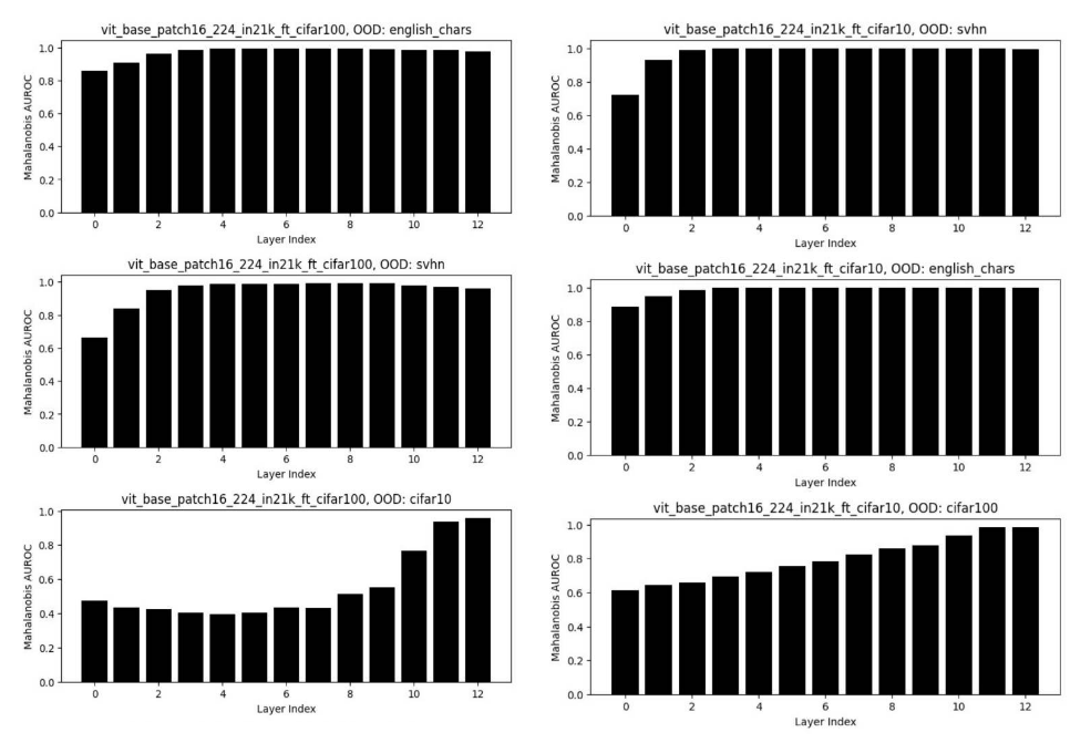
Fig. 6: Performance in OOD detection for the different layers of the ViT models. We can observe that the last layer always yield very good OOD detection performance making aggregation methods (other than just selecting the last layer) somewhat irrelevant or at least not better than the usual heuristic.

References

- Amer et al. (2013) Amer, M., Goldstein, M., and Abdennadher, S. Enhancing one-class support vector machines for unsupervised anomaly detection. In Proceedings of the ACM SIGKDD workshop on outlier detection and description, pp. 8–15, 2013.
- Arora et al. (2020) Arora, G., Jain, C., Chaturvedi, M., and Modi, K. HINT3: Raising the bar for intent detection in the wild. In Proceedings of the First Workshop on Insights from Negative Results in NLP, pp. 100–105, Online, November 2020. Association for Computational Linguistics. doi: 10.18653/v1/2020.insights-1.16. URL https://www.aclweb.org/anthology/2020.insights-1.16.
- Arora et al. (2021) Arora, U., Huang, W., and He, H. Types of out-of-distribution texts and how to detect them. arXiv preprint arXiv:2109.06827, 2021.
- Artetxe et al. (2019) Artetxe, M., Ruder, S., and Yogatama, D. On the cross-lingual transferability of monolingual representations. CoRR, abs/1910.11856, 2019.
- Baheti et al. (2021) Baheti, A., Sap, M., Ritter, A., and Riedl, M. Just say no: Analyzing the stance of neural dialogue generation in offensive contexts. arXiv preprint arXiv:2108.11830, 2021.
- Barbieri et al. (2022) Barbieri, F., Espinosa Anke, L., and Camacho-Collados, J. XLM-T: Multilingual language models in Twitter for sentiment analysis and beyond. In Proceedings of the Thirteenth Language Resources and Evaluation Conference, pp. 258–266, Marseille, France, June 2022. European Language Resources Association. URL https://aclanthology.org/2022.lrec-1.27.
- Berend et al. (2020) Berend, D., Xie, X., Ma, L., Zhou, L., Liu, Y., Xu, C., and Zhao, J. Cats are not fish: Deep learning testing calls for out-of-distribution awareness. In Proceedings of the 35th IEEE/ACM International Conference on Automated Software Engineering, pp. 1041–1052, 2020.
- Blard (2019) Blard, T. French sentiment analysis with bert. https://github.com/TheophileBlard/french-sentiment-analysis-with-bert, 2019.
- Bradley (1997) Bradley, A. P. The use of the area under the roc curve in the evaluation of machine learning algorithms. Pattern recognition, 30(7):1145–1159, 1997.
- Breunig et al. (2000) Breunig, M. M., Kriegel, H.-P., Ng, R. T., and Sander, J. Lof: identifying density-based local outliers. In Proceedings of the 2000 ACM SIGMOD international conference on Management of data, pp. 93–104, 2000.
- Bulusu et al. (2020) Bulusu, S., Kailkhura, B., Li, B., Varshney, P. K., and Song, D. Anomalous example detection in deep learning: A survey. IEEE Access, 8:132330–132347, 2020.
- Burger & Ferro (2005) Burger, J. and Ferro, L. Generating an entailment corpus from news headlines. In Proceedings of the ACL Workshop on Empirical Modeling of Semantic Equivalence and Entailment, pp. 49–54. Association for Computational Linguistics, 2005.
- Casanueva et al. (2020) Casanueva, I., Temcinas, T., Gerz, D., Henderson, M., and Vulic, I. Efficient intent detection with dual sentence encoders. In Proceedings of the 2nd Workshop on NLP for ConvAI - ACL 2020, mar 2020. URL https://arxiv.org/abs/2003.04807. Data available at https://github.com/PolyAI-LDN/task-specific-datasets.
- Chapuis* et al. (2020a) Chapuis*, E., Colombo*, P., Manica, M., Labeau, M., and Clavel, C. Hierarchical pre-training for sequence labelling in spoken dialog. Finding of EMNLP 2020, 2020a.
- Chapuis* et al. (2020b) Chapuis*, E., Colombo*, P., Manica, M., Varni, G., Vignon, E., and Clavel, C. Guider l’attention dans les modèles de séquence à séquence pour la prédiction des actes de dialogue. In WACAI 2020, 2020b.
- Colombo (2021a) Colombo, P. Apprendre à représenter et à générer du texte en utilisant des mesures d’information. PhD thesis, (PhD thesis) Institut Polytechnique de Paris, 2021a.
- Colombo (2021b) Colombo, P. Learning to represent and generate text using information measures. PhD thesis, (PhD thesis) Institut polytechnique de Paris, 2021b.
- Colombo* et al. (2019) Colombo*, P., Witon*, W., Modi, A., Kennedy, J., and Kapadia, M. Affect-driven dialog generation. NAACL 2019, 2019.
- Colombo* et al. (2020) Colombo*, P., Chapuis*, E., Manica, M., Vignon, E., Varni, G., and Clavel, C. Guiding attention in sequence-to-sequence models for dialogue act prediction. AAAI 2020, 2020.
- Colombo et al. (2021a) Colombo, P., Chapuis, E., Labeau, M., and Clavel, C. Code-switched inspired losses for spoken dialog representations. In EMNLP 2021, 2021a.
- Colombo et al. (2021b) Colombo, P., Chapuis, E., Labeau, M., and Clavel, C. Improving multimodal fusion via mutual dependency maximisation. EMNLP 2021, 2021b.
- Colombo et al. (2021c) Colombo, P., Clave, C., and Piantanida, P. Infolm: A new metric to evaluate summarization & data2text generation. AAAI 2022, 2021c.
- Colombo et al. (2021d) Colombo, P., Clavel, C., and Piantanida, P. A novel estimator of mutual information for learning to disentangle textual representations. ACL 2021, 2021d.
- Colombo et al. (2021e) Colombo, P., Yang, C., Varni, G., and Clavel, C. Beam search with bidirectional strategies for neural response generation. ICNLSP 2021, 2021e.
- Colombo et al. (2022a) Colombo, P., Gomes, E. D. C., Staerman, G., Noiry, N., and Piantanida, P. Beyond mahalanobis distance for textual ood detection. In Advances in Neural Information Processing Systems, 2022a.
- Colombo et al. (2022b) Colombo, P., Noiry, N., Irurozki, E., and Clémençon, S. What are the best systems? new perspectives on nlp benchmarking. NeurIPS 2022, 2022b.
- Conneau et al. (2018) Conneau, A., Rinott, R., Lample, G., Williams, A., Bowman, S. R., Schwenk, H., and Stoyanov, V. Xnli: Evaluating cross-lingual sentence representations. In Proceedings of the 2018 Conference on Empirical Methods in Natural Language Processing. Association for Computational Linguistics, 2018.
- Dara & Tumma (2018) Dara, S. and Tumma, P. Feature extraction by using deep learning: A survey. In 2018 Second International Conference on Electronics, Communication and Aerospace Technology (ICECA), pp. 1795–1801, 2018. doi: 10.1109/ICECA.2018.8474912.
- Darrin et al. (2022) Darrin, M., Piantanida, P., and Colombo, P. Rainproof: An umbrella to shield text generators from out-of-distribution data. arXiv preprint arXiv:2212.09171, 2022.
- Davis & Goadrich (2006) Davis, J. and Goadrich, M. The relationship between precision-recall and roc curves. In Proceedings of the 23rd international conference on Machine learning, pp. 233–240, 2006.
- de Vries et al. (2020) de Vries, W., van Cranenburgh, A., and Nissim, M. What’s so special about bert’s layers? a closer look at the nlp pipeline in monolingual and multilingual models. arXiv preprint arXiv:2004.06499, 2020.
- Demszky et al. (2020) Demszky, D., Movshovitz-Attias, D., Ko, J., Cowen, A., Nemade, G., and Ravi, S. GoEmotions: A Dataset of Fine-Grained Emotions. In 58th Annual Meeting of the Association for Computational Linguistics (ACL), 2020.
- Deng et al. (2009) Deng, J., Dong, W., Socher, R., Li, L.-J., Li, K., and Fei-Fei, L. ImageNet: A Large-Scale Hierarchical Image Database. In CVPR09, 2009.
- Devlin et al. (2018) Devlin, J., Chang, M.-W., Lee, K., and Toutanova, K. Bert: Pre-training of deep bidirectional transformers for language understanding. arXiv preprint arXiv:1810.04805, 2018.
- Dinkar* et al. (2020) Dinkar*, T., Colombo*, P., Labeau, M., and Clavel, C. The importance of fillers for text representations of speech transcripts. EMNLP 2020, 2020.
- Esmaeilpour et al. (2022) Esmaeilpour, S., Liu, B., Robertson, E., and Shu, L. Zero-shot out-of-distribution detection based on the pretrained model clip. In Proceedings of the AAAI conference on artificial intelligence, 2022.
- Fang & Zhan (2015) Fang, X. and Zhan, J. Sentiment analysis using product review data. Journal of Big Data, 2(1):1–14, 2015.
- Fang et al. (2022) Fang, Z., Li, Y., Lu, J., Dong, J., Han, B., and Liu, F. Is out-of-distribution detection learnable? In Oh, A. H., Agarwal, A., Belgrave, D., and Cho, K. (eds.), Advances in Neural Information Processing Systems, 2022. URL https://openreview.net/forum?id=sde_7ZzGXOE.
- FitzGerald et al. (2022) FitzGerald, J., Hench, C., Peris, C., Mackie, S., Rottmann, K., Sanchez, A., Nash, A., Urbach, L., Kakarala, V., Singh, R., Ranganath, S., Crist, L., Britan, M., Leeuwis, W., Tur, G., and Natarajan, P. Massive: A 1m-example multilingual natural language understanding dataset with 51 typologically-diverse languages, 2022.
- Garcia* et al. (2019) Garcia*, A., Colombo*, P., Essid, S., d’Alché Buc, F., and Clavel, C. From the token to the review: A hierarchical multimodal approach to opinion mining. EMNLP 2019, 2019.
- (41) Gomes, E. D. C., Colombo, P., Staerman, G., Noiry, N., and Piantanida, P. A functional perspective on multi-layer out-of-distribution detection.
- Gomes et al. (2022) Gomes, E. D. C., Alberge, F., Duhamel, P., and Piantanida, P. Igeood: An information geometry approach to out-of-distribution detection. arXiv preprint arXiv:2203.07798, 2022.
- Guerreiro et al. (2023) Guerreiro, N. M., Colombo, P., Piantanida, P., and Martins, A. F. Optimal transport for unsupervised hallucination detection in neural machine translation. arXiv preprint arXiv:2212.09631, 2023.
- Hardy et al. (1952) Hardy, G. H., Littlewood, J. E., Pólya, G., Pólya, G., et al. Inequalities. Cambridge university press, 1952.
- Hariri et al. (2019) Hariri, S., Kind, M. C., and Brunner, R. J. Extended isolation forest. IEEE Transactions on Knowledge and Data Engineering, 33(4):1479–1489, 2019.
- Hendrycks & Gimpel (2016) Hendrycks, D. and Gimpel, K. A baseline for detecting misclassified and out-of-distribution examples in neural networks. arXiv preprint arXiv:1610.02136, 2016.
- Hendrycks et al. (2020) Hendrycks, D., Liu, X., Wallace, E., Dziedzic, A., Krishnan, R., and Song, D. Pretrained transformers improve out-of-distribution robustness. arXiv preprint arXiv:2004.06100, 2020.
- Hickl et al. (2006) Hickl, A., Williams, J., Bensley, J., Roberts, K., Rink, B., and Shi, Y. Recognizing textual entailment with lcc’s groundhog system. In Proceedings of the Second PASCAL Challenges Workshop, 2006.
- Hovy et al. (2001) Hovy, E., Gerber, L., Hermjakob, U., Lin, C.-Y., and Ravichandran, D. Toward semantics-based answer pinpointing. In Proceedings of the First International Conference on Human Language Technology Research, 2001. URL https://www.aclweb.org/anthology/H01-1069.
- Huang et al. (2020) Huang, H., Li, Z., Wang, L., Chen, S., Dong, B., and Zhou, X. Feature space singularity for out-of-distribution detection. arXiv preprint arXiv:2011.14654, 2020.
- Huang & Li (2021) Huang, R. and Li, Y. Mos: Towards scaling out-of-distribution detection for large semantic space. In Proceedings of the IEEE/CVF Conference on Computer Vision and Pattern Recognition, pp. 8710–8719, 2021.
- (52) Huang, W., Wang, H., Xia, J., Wang, C., and Zhang, J. Density-driven regularization for out-of-distribution detection. In Advances in Neural Information Processing Systems.
- Ilin et al. (2017) Ilin, R., Watson, T., and Kozma, R. Abstraction hierarchy in deep learning neural networks. In 2017 International Joint Conference on Neural Networks (IJCNN), pp. 768–774. IEEE, 2017.
- Jakubovitz et al. (2019) Jakubovitz, D., Giryes, R., and Rodrigues, M. R. Generalization error in deep learning. In Compressed sensing and its applications, pp. 153–193. Springer, 2019.
- Jalalzai* et al. (2020) Jalalzai*, H., Colombo*, P., Clavel, C., Gaussier, É., Varni, G., Vignon, E., and Sabourin, A. Heavy-tailed representations, text polarity classification & data augmentation. NeurIPS 2020, 2020.
- Joachims (1996) Joachims, T. A probabilistic analysis of the rocchio algorithm with tfidf for text categorization. Technical report, Carnegie-mellon univ pittsburgh pa dept of computer science, 1996.
- Khalid et al. (2022) Khalid, U., Esmaeili, A., Karim, N., and Rahnavard, N. Rodd: A self-supervised approach for robust out-of-distribution detection. arXiv preprint arXiv:2204.02553, 2022.
- Kharde et al. (2016) Kharde, V., Sonawane, P., et al. Sentiment analysis of twitter data: a survey of techniques. arXiv preprint arXiv:1601.06971, 2016.
- Kirichenko et al. (2020) Kirichenko, P., Izmailov, P., and Wilson, A. G. Why normalizing flows fail to detect out-of-distribution data. In Advances in Neural Information Processing Systems, volume 33, pp. 20578–20589. Curran Associates, Inc., 2020.
- Kozma et al. (2018) Kozma, R., Ilin, R., and Siegelmann, H. T. Evolution of abstraction across layers in deep learning neural networks. Procedia Computer Science, 144:203–213, 2018. ISSN 1877-0509. doi: https://doi.org/10.1016/j.procs.2018.10.520.
- Lang (1995) Lang, K. Newsweeder: Learning to filter netnews. In Prieditis, A. and Russell, S. (eds.), Machine Learning Proceedings 1995, pp. 331–339. Morgan Kaufmann, San Francisco (CA), 1995. ISBN 978-1-55860-377-6. doi: https://doi.org/10.1016/B978-1-55860-377-6.50048-7. URL https://www.sciencedirect.com/science/article/pii/B9781558603776500487.
- Larson et al. (2019) Larson, S., Mahendran, A., Peper, J. J., Clarke, C., Lee, A., Hill, P., Kummerfeld, J. K., Leach, K., Laurenzano, M. A., Tang, L., et al. An evaluation dataset for intent classification and out-of-scope prediction. arXiv preprint arXiv:1909.02027, 2019.
- Le & Yang (2015) Le, Y. and Yang, X. Tiny imagenet visual recognition challenge. 2015.
- Lee et al. (2022) Lee, J., Prabhushankar, M., and AlRegib, G. Gradient-based adversarial and out-of-distribution detection. arXiv preprint arXiv:2206.08255, 2022.
- Lee et al. (2018) Lee, K., Lee, K., Lee, H., and Shin, J. A simple unified framework for detecting out-of-distribution samples and adversarial attacks. Advances in neural information processing systems, 31, 2018.
- Lhoest et al. (2021) Lhoest, Q., Villanova del Moral, A., Jernite, Y., Thakur, A., von Platen, P., Patil, S., Chaumond, J., Drame, M., Plu, J., Tunstall, L., Davison, J., Šaško, M., Chhablani, G., Malik, B., Brandeis, S., Le Scao, T., Sanh, V., Xu, C., Patry, N., McMillan-Major, A., Schmid, P., Gugger, S., Delangue, C., Matussière, T., Debut, L., Bekman, S., Cistac, P., Goehringer, T., Mustar, V., Lagunas, F., Rush, A., and Wolf, T. Datasets: A community library for natural language processing. In Proceedings of the 2021 Conference on Empirical Methods in Natural Language Processing: System Demonstrations, pp. 175–184, Online and Punta Cana, Dominican Republic, November 2021. Association for Computational Linguistics. URL https://aclanthology.org/2021.emnlp-demo.21.
- Li & Roth (2002) Li, X. and Roth, D. Learning question classifiers. In COLING 2002: The 19th International Conference on Computational Linguistics, 2002. URL https://aclanthology.org/C02-1150.
- Li et al. (2021) Li, X., Li, J., Sun, X., Fan, C., Zhang, T., Wu, F., Meng, Y., and Zhang, J. folden: -fold ensemble for out-of-distribution detection. arXiv preprint arXiv:2108.12731, 2021.
- Liang et al. (2017) Liang, S., Li, Y., and Srikant, R. Enhancing the reliability of out-of-distribution image detection in neural networks. arXiv preprint arXiv:1706.02690, 2017.
- Liang et al. (2018) Liang, S., Li, Y., and Srikant, R. Enhancing the reliability of out-of-distribution image detection in neural networks. In International Conference on Learning Representations, 2018. URL https://openreview.net/forum?id=H1VGkIxRZ.
- Liu et al. (2008) Liu, F. T., Ting, K. M., and Zhou, Z.-H. Isolation forest. In In Proceedings 8th IEEE International Conference on Data Mining, pp. 413–422, 2008.
- Liu et al. (2020) Liu, W., Wang, X., Owens, J., and Li, Y. Energy-based out-of-distribution detection. Advances in Neural Information Processing Systems, 2020.
- Liu et al. (2019) Liu, Y., Ott, M., Goyal, N., Du, J., Joshi, M., Chen, D., Levy, O., Lewis, M., Zettlemoyer, L., and Stoyanov, V. Roberta: A robustly optimized bert pretraining approach. arXiv preprint arXiv:1907.11692, 2019.
- Lundberg & Lee (2017) Lundberg, S. M. and Lee, S.-I. A unified approach to interpreting model predictions. In Guyon, I., Luxburg, U. V., Bengio, S., Wallach, H., Fergus, R., Vishwanathan, S., and Garnett, R. (eds.), Advances in Neural Information Processing Systems 30, pp. 4765–4774. Curran Associates, Inc., 2017.
- Maas et al. (2011) Maas, A. L., Daly, R. E., Pham, P. T., Huang, D., Ng, A. Y., and Potts, C. Learning word vectors for sentiment analysis. In Proceedings of the 49th Annual Meeting of the Association for Computational Linguistics: Human Language Technologies, pp. 142–150, Portland, Oregon, USA, June 2011. Association for Computational Linguistics. URL https://aclanthology.org/P11-1015.
- McAllister et al. (2019) McAllister, R., Kahn, G., Clune, J., and Levine, S. Robustness to out-of-distribution inputs via task-aware generative uncertainty. In 2019 International Conference on Robotics and Automation (ICRA), pp. 2083–2089. IEEE, 2019.
- Modi et al. (2020) Modi, A., Kapadia, M., Fidaleo, D. A., Kennedy, J. R., Witon, W., and Colombo, P. Affect-driven dialog generation, October 27 2020. US Patent 10,818,312.
- Niklaus et al. (2022) Niklaus, J., Stürmer, M., and Chalkidis, I. An empirical study on cross-x transfer for legal judgment prediction, 2022.
- Pearce et al. (2021) Pearce, T., Brintrup, A., and Zhu, J. Understanding softmax confidence and uncertainty. arXiv preprint arXiv:2106.04972, 2021.
- Pichler et al. (2022) Pichler, G., Colombo, P. J. A., Boudiaf, M., Koliander, G., and Piantanida, P. A differential entropy estimator for training neural networks. In ICML 2022, 2022.
- Picot et al. (2023a) Picot, M., Noiry, N., Piantanida, P., and Colombo, P. Adversarial attack detection under realistic constraints. 2023a.
- Picot et al. (2023b) Picot, M., Staerman, G., Granese, F., Noiry, N., Messina, F., Piantanida, P., and Colombo, P. A simple unsupervised data depth-based method to detect adversarial images. 2023b.
- Podolskiy et al. (2021) Podolskiy, A., Lipin, D., Bout, A., Artemova, E., and Piontkovskaya, I. Revisiting mahalanobis distance for transformer-based out-of-domain detection. arXiv preprint arXiv:2101.03778, 2021.
- Raghuram et al. (2021) Raghuram, J., Chandrasekaran, V., Jha, S., and Banerjee, S. A general framework for detecting anomalous inputs to dnn classifiers. In International Conference on Machine Learning, pp. 8764–8775. PMLR, 2021.
- Ramsay et al. (2019) Ramsay, K., Durocher, S., and Leblanc, A. Integrated rank-weighted depth. Journal of Multivariate Analysis, 173:51–69, 2019.
- Ren et al. (2019) Ren, J., Liu, P. J., Fertig, E., Snoek, J., Poplin, R., Depristo, M., Dillon, J., and Lakshminarayanan, B. Likelihood ratios for out-of-distribution detection. In Advances in Neural Information Processing Systems, volume 32. Curran Associates, Inc., 2019.
- Rücklé et al. (2018) Rücklé, A., Eger, S., Peyrard, M., and Gurevych, I. Concatenated power mean word embeddings as universal cross-lingual sentence representations. arXiv preprint arXiv:1803.01400, 2018.
- Ruder (2022) Ruder, S. The State of Multilingual AI. http://ruder.io/state-of-multilingual-ai/, 2022.
- Sanh et al. (2019) Sanh, V., Debut, L., Chaumond, J., and Wolf, T. Distilbert, a distilled version of bert: smaller, faster, cheaper and lighter. arXiv preprint arXiv:1910.01108, 2019.
- Sastry & Oore (2020) Sastry, C. S. and Oore, S. Detecting out-of-distribution examples with gram matrices. In International Conference on Machine Learning, pp. 8491–8501. PMLR, 2020.
- Schwinn et al. (2021) Schwinn, L., Nguyen, A., Raab, R., Bungert, L., Tenbrinck, D., Zanca, D., Burger, M., and Eskofier, B. Identifying untrustworthy predictions in neural networks by geometric gradient analysis. In Uncertainty in Artificial Intelligence, pp. 854–864. PMLR, 2021.
- Serrà et al. (2019) Serrà, J., Álvarez, D., Gómez, V., Slizovskaia, O., Núñez, J. F., and Luque, J. Input complexity and out-of-distribution detection with likelihood-based generative models. arXiv preprint arXiv:1909.11480, 2019.
- Socher et al. (2013) Socher, R., Perelygin, A., Wu, J., Chuang, J., Manning, C. D., Ng, A., and Potts, C. Recursive deep models for semantic compositionality over a sentiment treebank. In Proceedings of the 2013 Conference on Empirical Methods in Natural Language Processing, pp. 1631–1642, Seattle, Washington, USA, October 2013. Association for Computational Linguistics. URL https://aclanthology.org/D13-1170.
- Srinivasan et al. (2021) Srinivasan, A., Sitaram, S., Ganu, T., Dandapat, S., Bali, K., and Choudhury, M. Predicting the performance of multilingual nlp models. arXiv preprint arXiv:2110.08875, 2021.
- Staerman et al. (2019) Staerman, G., Mozharovskyi, P., Clémençon, S., and d’Alché Buc, F. Functional isolation forest. In Proceedings of The Eleventh Asian Conference on Machine Learning, pp. 332–347, 2019.
- Staerman et al. (2021a) Staerman, G., Mozharovskyi, P., and Clémençon, S. Affine-invariant integrated rank-weighted depth: Definition, properties and finite sample analysis. arXiv preprint arXiv:2106.11068, 2021a.
- Staerman et al. (2021b) Staerman, G., Mozharovskyi, P., Colombo, P., Clémençon, S., and d’Alché Buc, F. A pseudo-metric between probability distributions based on depth-trimmed regions. arXiv e-prints, pp. arXiv–2103, 2021b.
- Sun et al. (2022) Sun, Y., Ming, Y., Zhu, X., and Li, Y. Out-of-distribution detection with deep nearest neighbors. In ICML, 2022.
- Techapanurak et al. (2019) Techapanurak, E., Suganuma, M., and Okatani, T. Hyperparameter-free out-of-distribution detection using softmax of scaled cosine similarity. arXiv preprint arXiv:1905.10628, 2019.
- Vamvas & Sennrich (2020) Vamvas, J. and Sennrich, R. X-stance: A multilingual multi-target dataset for stance detection. arXiv preprint arXiv:2003.08385, 2020.
- van Esch et al. (2022) van Esch, D., Lucassen, T., Ruder, S., Caswell, I., and Rivera, C. Writing system and speaker metadata for 2,800+ language varieties. In Proceedings of the Thirteenth Language Resources and Evaluation Conference, pp. 5035–5046, 2022.
- Vaswani et al. (2017) Vaswani, A., Shazeer, N., Parmar, N., Uszkoreit, J., Jones, L., Gomez, A. N., Kaiser, Ł., and Polosukhin, I. Attention is all you need. Advances in neural information processing systems, 30, 2017.
- Vyas et al. (2018) Vyas, A., Jammalamadaka, N., Zhu, X., Das, D., Kaul, B., and Willke, T. L. Out-of-distribution detection using an ensemble of self supervised leave-out classifiers. In Proceedings of the European Conference on Computer Vision (ECCV), pp. 550–564, 2018.
- Wang et al. (2018) Wang, A., Singh, A., Michael, J., Hill, F., Levy, O., and Bowman, S. R. Glue: A multi-task benchmark and analysis platform for natural language understanding. arXiv preprint arXiv:1804.07461, 2018.
- Wang et al. (2019) Wang, A., Pruksachatkun, Y., Nangia, N., Singh, A., Michael, J., Hill, F., Levy, O., and Bowman, S. R. Superglue: A stickier benchmark for general-purpose language understanding systems. arXiv preprint arXiv:1905.00537, 2019.
- Wang et al. (2022a) Wang, H., Li, Z., Feng, L., and Zhang, W. Vim: Out-of-distribution with virtual-logit matching. In Proceedings of the IEEE/CVF Conference on Computer Vision and Pattern Recognition, pp. 4921–4930, 2022a.
- Wang et al. (2022b) Wang, H., Zhao, C., Zhao, X., and Chen, F. Layer adaptive deep neural networks for out-of-distribution detection. In Advances in Knowledge Discovery and Data Mining: 26th Pacific-Asia Conference, PAKDD 2022, Chengdu, China, May 16–19, 2022, Proceedings, Part II, pp. 526–538. Springer, 2022b.
- (108) Wang, Y., Zou, J., Lin, J., Ling, Q., Pan, Y., Yao, T., and Mei, T. Out-of-distribution detection via conditional kernel independence model. In Advances in Neural Information Processing Systems.
- Williams et al. (2018) Williams, A., Nangia, N., and Bowman, S. A broad-coverage challenge corpus for sentence understanding through inference. In Proceedings of the 2018 Conference of the North American Chapter of the Association for Computational Linguistics: Human Language Technologies, Volume 1 (Long Papers), pp. 1112–1122, New Orleans, Louisiana, June 2018. Association for Computational Linguistics. doi: 10.18653/v1/N18-1101. URL https://aclanthology.org/N18-1101.
- Winkens et al. (2020a) Winkens, J., Bunel, R., Roy, A. G., Stanforth, R., Natarajan, V., Ledsam, J. R., MacWilliams, P., Kohli, P., Karthikesalingam, A., Kohl, S., et al. Contrastive training for improved out-of-distribution detection. arXiv preprint arXiv:2007.05566, 2020a.
- Winkens et al. (2020b) Winkens, J., Bunel, R., Roy, A. G., Stanforth, R., Natarajan, V., Ledsam, J. R., MacWilliams, P., Kohli, P., Karthikesalingam, A., Kohl, S. A. A., taylan. cemgil, Eslami, S. M. A., and Ronneberger, O. Contrastive training for improved out-of-distribution detection. ArXiv, abs/2007.05566, 2020b.
- Witon* et al. (2018) Witon*, W., Colombo*, P., Modi, A., and Kapadia, M. Disney at iest 2018: Predicting emotions using an ensemble. In Wassa @EMNP2018, 2018.
- Xu et al. (2020) Xu, H., He, K., Yan, Y., Liu, S., Liu, Z., and Xu, W. A deep generative distance-based classifier for out-of-domain detection with mahalanobis space. In Proceedings of the 28th International Conference on Computational Linguistics, pp. 1452–1460, 2020.
- Yang et al. (2021) Yang, J., Zhou, K., Li, Y., and Liu, Z. Generalized out-of-distribution detection: A survey, 2021. URL https://arxiv.org/abs/2110.11334.
- Yang et al. (2019) Yang, Y., Zhang, Y., Tar, C., and Baldridge, J. PAWS-X: A Cross-lingual Adversarial Dataset for Paraphrase Identification. In Proc. of EMNLP, 2019.
- Zhang et al. (2022) Zhang, Q., Shen, X., Chang, E., Ge, J., and Chen, P. Mdia: A benchmark for multilingual dialogue generation in 46 languages. arXiv preprint arXiv:2208.13078, 2022.
- Zhou et al. (2021) Zhou, W., Liu, F., and Chen, M. Contrastive out-of-distribution detection for pretrained transformers. arXiv preprint arXiv:2104.08812, 2021.
- Zotova et al. (2020) Zotova, E., Agerri, R., Nuñez, M., and Rigau, G. Multilingual stance detection in tweets: The Catalonia independence corpus. In Proceedings of the Twelfth Language Resources and Evaluation Conference, pp. 1368–1375, Marseille, France, May 2020. European Language Resources Association. ISBN 979-10-95546-34-4. URL https://aclanthology.org/2020.lrec-1.171.