Transductive Matrix Completion with Calibration for Multi-Task Learning

Abstract

Multi-task learning has attracted much attention due to growing multi-purpose research with multiple related data sources. Moreover, transduction with matrix completion is a useful method in multi-label learning. In this paper, we propose a transductive matrix completion algorithm that incorporates a calibration constraint for the features under the multi-task learning framework. The proposed algorithm recovers the incomplete feature matrix and target matrix simultaneously. Fortunately, the calibration information improves the completion results. In particular, we provide a statistical guarantee for the proposed algorithm, and the theoretical improvement induced by calibration information is also studied. Moreover, the proposed algorithm enjoys a sub-linear convergence rate. Several synthetic data experiments are conducted, which show the proposed algorithm out-performs other existing methods, especially when the target matrix is associated with the feature matrix in a nonlinear way.

1 Introduction

With the advent of the big data era, massive amounts of information and data have been collected by modern high-tech devices, including web servers, environmental sensors, x-ray imaging machines, and so on. Based on multiple data sources related to learning purposes, algorithms have been developed to achieve various learning goals. Multi-task learning (MTL) [1], for example, implements a robust learner for multiple tasks incorporating multiple sources, and it can be widely used in practice, including web search, medical diagnosis, natural language processing, and computer version.

MTL has advantages for analyzing the multi-response structure. For $i=1,\ldots,n$, let $\mathbf{y}_{i}\in\mathbb{R}^{m}$ be the vector of interest of length $m$, where $n$ is the number of instances, and each element corresponds to a particular task. Denote $\mathbf{Y}=(y_{ij})$ to be the $n\times m$ response matrix, consisting of the $n$ realizations of $\mathbf{y}_{i}$. If the responses for a specific task are categorical, it is essentially a multi-label learning problem. As for continuous responses, it turns out to be a multi-response regression problem if additional features are available. As the exponential family is flexible to handle different data types, regardless of categorical or continuous, for each task, we assume that $y_{ij}$ independently comes from an exponential family distribution with parameter $z_{\star,ij}$, which forms $\mathbf{Z}_{\star}=(z_{\star,ij})$. The goal is to learn the underlying $\mathbf{Z}_{\star}$ based on $\mathbf{Y}$. Moreover, entries of $\mathbf{Y}$ may suffer from missingness which makes it difficult to learn $\mathbf{Z}_{\star}$. To tackle this difficulty and estimate $\mathbf{Z}_{\star}$ simultaneously, matrix completion (MC) [2, 3, 4, 5, 6] algorithms have been developed under the low-rank and other regularity assumptions. The recovery of the target matrix without any additional features is studied in [7]. Noisy MC is investigated in [8, 9] from the exponential family with fully observed features.

In MTL problems, features related to the responses may exist, but it is inevitable that such features also suffer from missingness. Goldberg et al. (2010) [10] studied such a problem under multi-label learning. Specifically, they studied single-task binary response matrix given feature matrix where both matrices were subject to missingness. Xu et al. (2018) [11] proposed the co-completion method by additionally penalizing the trace norm of the feature matrix. A recent work [12] considered this problem via a smoothed rank function approach. Under the noiseless case, [13] studied the error rate in the scenario with corrupted side information.

Calibration [14, 15, 16] is widely used to incorporate such prior knowledge in the learning procedure, and it improves the estimation efficiency. In this vein, [17] studied the calibration with local polynomial regression between responses and features. Later, [18] generalized this idea to the so-called model calibration under a parametric framework. Afterward, [19] generalized the idea to a functional type calibration equation. As far as we know, no calibration related work has been done under the MC framework.

In this paper, we focus on MTL problems incorporating incomplete features, and we assume that certain prior knowledge about the features is also available. Our work can be embodied in the following toy example. For the well-known Netflix movie rating problem [20], we aim to simultaneously complete rating and like-dislike matrices incorporating an incomplete feature matrix, consisting of age, gender, and so on. However, all three matrices suffer from missingness. When additional information such as the summary statistics for age, gender, etc., can be obtained from the census survey, we investigate the benefits of such additional information incorporated by the calibration method. In a nutshell, we propose a Transductive Matrix Completion with Calibration (TMCC) algorithm, and the prior information about the features is considered by an additional calibration constraint. As far as we know, this is the first paper exploring multi-task learning under a matrix completion framework with calibration. Methodologically, our method has two merits: (i) the target and feature matrices can be completed simultaneously; (ii) calibration information can be incorporated. Theoretically, we show the statistical guarantee of our method, and the benefit of calibration is also discussed. Besides, we have validated that the convergence rate of the proposed algorithm is $O(1/k^{2})$. Numerically, synthetic data experiments show that our proposed method performs better than other existing methods, especially when the target matrix has a nonlinear transformation from the feature matrix.

Notations. Denote $[n]$ as the set $\{1,\ldots,n\}$. Given an arbitrary matrix $\mathbf{S}=(s_{ij})\in\mathbb{R}^{n_{1}\times n_{2}}$, the Frobenius norm of $\mathbf{S}$ is $\left\|\mathbf{S}\right\|_{F}=(\sum_{i=1}^{n_{1}}\sum_{j=1}^{n_{2}}s_{ij}^{2})^{1/2}$. Denote the singular values of $\mathbf{S}$ as $\sigma_{1}(\mathbf{S}),\ldots,\sigma_{n_{1}\wedge n_{2}}(\mathbf{S})$ in descending order. The operator norm is $\|\mathbf{S}\|=\sigma_{\max}(\mathbf{S})=\sigma_{1}(\mathbf{S})$ and the nuclear norm $\|\mathbf{S}\|_{\star}=\sum_{i=1}^{n_{1}\wedge n_{2}}\sigma_{i}(\mathbf{S})$. Besides, let $\sigma_{\min}(\mathbf{S})=\sigma_{n_{1}\wedge n_{2}}(\mathbf{S})$.

2 Model and Algorithm

Suppose there are $S$ response matrices, $\mathbf{Y}^{(1)},\ldots,\mathbf{Y}^{(S)}$. For example, $\mathbf{Y}^{(1)}$ can be a like-dislike matrix, and $\mathbf{Y}^{(2)}$ can be a rating matrix, whose rows correspond to users, columns correspond to movies, and $S=2$. Denote the number of instances by $n$, the number of tasks for $s$-th response matrix by $m_{s}$. For $s\in[S]$, we have $\mathbf{Y}^{(s)}=(y_{ij}^{(s)})\in\mathbb{R}^{n\times m_{s}}$, and $y_{ij}^{(s)}$ can be either discrete or continuous for $i\in[n]$. We assume that within the same response matrix, all entries follow the same generic exponential family. For example, all entries of $\mathbf{Y}^{(1)}$ follow Bernoulli distributions with different success probabilities. Let $\mathbf{R}_{y}^{(s)}=(r_{y,ij}^{(s)})\in\mathbb{R}^{n\times m_{s}}$ be the corresponding indicator matrix for $\mathbf{Y}^{(s)}$. In particular, if $y_{ij}^{(s)}$ is observed, then $r_{y,ij}^{(s)}=1$; otherwise, $r_{y,ij}^{(s)}=0$. Furthermore, assume that $\mathbf{Y}^{(s)}$ is generated from a low-rank matrix $\mathbf{Z}_{\star}^{(s)}=(z_{\star,ij}^{(s)})\in\mathbb{R}^{n\times m_{s}}$ by the exponential family via a base function $h^{(s)}$ and a link function $g^{(s)}$, namely, the density function $f^{(s)}(y_{ij}^{(s)}|z_{\star,ij}^{(s)})=h^{(s)}(y_{ij}^{(s)})\exp\{y_{ij}^{(s)}z_{\star,ij}^{(s)}-g^{(s)}(z_{\star,ij}^{(s)})\}$, for $s\in[S]$. For instance, suppose $g^{(s)}(z_{\star,ij}^{(s)})=\sigma^{2}(z_{\star,ij}^{(s)})^{2}/2$ and $h^{(s)}(y_{ij}^{(s)})=(2\pi\sigma^{2})^{-1/2}\exp{\{-(y_{ij}^{(s)})^{2}/(2\sigma^{2})\}}$, and the corresponding exponential family is the Gaussian distribution with mean $\sigma^{2}z_{\star,ij}^{(s)}$ and variance $\sigma^{2}$ with support $\mathbb{R}$.

Denote $\mathbf{X}_{\star}=(x_{\star,ij})\in\mathbb{R}^{n\times d}$ as the true feature matrix consisting of $d$ feature, and it is assumed to be low-rank. Let $\mathbf{X}=(x_{ij})\in\mathbb{R}^{n\times d}$ be a noisy version of the true feature matrix, i.e., $\mathbf{X}=\mathbf{X}_{\star}+\boldsymbol{\epsilon}$, where $\boldsymbol{\epsilon}=(\epsilon_{ij})\in\mathbb{R}^{n\times d}$ is a noise matrix with $\mathbb{E}(\mathbb{\boldsymbol{\epsilon}})=\mathbf{0}$, and its entries are independent. As the feature matrix is also incomplete, in a similar fashion, we denote $\mathbf{R}_{x}=(r_{x,ij})\in\mathbb{R}^{n\times d}$ as the corresponding indicator matrix of $\mathbf{X}$. That is, we only observe an incomplete matrix $\mathbf{R}_{x}\circ\mathbf{X}$, where $\circ$ denotes the Hadamard product. Let target matrix $\mathbf{Z}_{\star}=[\mathbf{Z}_{\star}^{(1)},\ldots,\mathbf{Z}_{\star}^{(S)}]$ be the collection of hidden parameter matrices. Our goal is to recover $\mathbf{Z}_{\star}$. We believe that some hidden connection between $\mathbf{X}_{\star}$ and $\mathbf{Z}_{\star}$ may provide us benefits for MTL.

Our method can be illustrated in Fig 1, where $\mbox{logit}(p)=\log\{p/(1-p)\}$, for $p\in(0,1)$. In this example, we have three observed matrices whose entries are from Bernoulli, Gaussian, and Poisson distributions, correspondingly, and are subject to missingness. In addition, we have an incomplete feature matrix related to the target matrix and calibration information for the true feature matrix. By the proposed TMCC algorithm, we can complete the true feature matrix and target matrix simultaneously.

Figure 1: Algorithm Illustration, where a Question Mark Represents a Missing Value.

Given density functions $\{f^{(s)}\}_{s=1}^{S}$, or collection of $\{g^{(s)}\}_{s=1}^{S}$ and $\{h^{(s)}\}_{s=1}^{S}$, the negative quasi log-likelihood function for $\mathbf{Z}^{\dagger}$ is

$$\ell_{0}\left(\mathbf{Z}^{\dagger}\right)= -\sum_{s=1}^{S}\sum_{(i,j)\in[n]\times[m_{s}]}r_{y,ij}^{(s)}\log\left\{f^{(s)}(y_{ij}^{(s)}|z_{ij}^{\dagger(s)})\right\}$$

$$= \sum_{s=1}^{S}\sum_{(i,j)\in[n]\times[m_{s}]}r_{y,ij}^{(s)}\left[\left\{-y_{ij}^{(s)}z_{ij}^{\dagger(s)}+g^{(s)}\left(z_{ij}^{\dagger(s)}\right)\right\}+\log\left\{h^{(s)}(y_{ij}^{(s)})\right\}\right]$$ (1)

where $\mathbf{Z}^{\dagger}=[\mathbf{Z}^{\dagger(1)},\ldots,\mathbf{Z}^{\dagger(S)}]$ and $\mathbf{Z}^{\dagger(s)}=(z_{ij}^{\dagger(s)})\in\mathbb{R}^{n\times m_{s}}$. As the argument $\mathbf{Z}^{\dagger}$ is irrelevant with the second term of (2), we refine (2) as

$$\ell\left(\mathbf{Z}^{\dagger}\right)=\sum_{s=1}^{S}\sum_{(i,j)\in[n]\times[m_{s}]}r_{y,ij}^{(s)}\left\{-y_{ij}^{(s)}z_{ij}^{\dagger(s)}+g^{(s)}\left(z_{ij}^{\dagger(s)}\right)\right\}.$$

Let $\mathbf{Y}=[\mathbf{Y}^{(1)},\ldots,\mathbf{Y}^{(S)}]$ be the collection of each specific task, $D=d+\sum_{s=1}^{S}m_{s}$ and $\mathbf{M}_{\star}$ be the concatenated matrix $[\mathbf{X}_{\star},\mathbf{Z}_{\star}]\in\mathbb{R}^{n\times D}$. Suppose we have an additional calibration constraint $\mathbf{A}\mathbf{X}_{\star}=\mathbf{B}$, where $\mathbf{A}$ and $\mathbf{B}$ are available. To incorporate the calibration constraint, the estimation procedure can be formulated as

$$\widehat{\mathbf{M}} =\operatorname*{arg\,min}_{\mathbf{M}^{\dagger}\in\mathbb{R}^{n\times D}}\left[\frac{1}{nD}\left\{\ell\left(\mathbf{Z}^{\dagger}\right)+\frac{1}{2}\left\|\mathbf{R}_{x}\circ\left(\mathbf{X}^{\dagger}-\mathbf{X}\right)\right\|_{F}^{2}\right\}\right.$$

$$\left.\ \ \ \ \ \ \ \ \ \ \ \ \ \ \ \ \ \ \ \ \quad\quad+\tau_{1}\left\|\mathbf{A}\mathbf{X}^{\dagger}-\mathbf{B}\right\|_{F}^{2}+\tau_{2}\left\|\mathbf{M}^{\dagger}\right\|_{\star}\right]$$

$$=:\operatorname*{arg\,min}_{\mathbf{M}^{\dagger}\in\mathbb{R}^{n\times D}}f_{\tau_{1}}\left(\mathbf{M}^{\dagger}\right)+\tau_{2}\left\|\mathbf{M}^{\dagger}\right\|_{\star}$$

$$=:\operatorname*{arg\,min}_{\mathbf{M}^{\dagger}\in\mathbb{R}^{n\times D}}\mathcal{L}_{\tau_{1},\tau_{2}}\left(\mathbf{M}^{\dagger}\right),$$ (2)

where $\mathbf{M}^{\dagger}=[\mathbf{X}^{\dagger},\mathbf{Z}^{\dagger}]$, $\widehat{\mathbf{M}}=[\widehat{\mathbf{X}},\widehat{\mathbf{Z}}]$ and we employ the commonly used square loss to complete the feature part. One trivial case is that when the calibration information is strong enough, i.e., $\mathbf{A}$ is invertible, the feature matrix $\mathbf{X}_{\star}$ can be exactly recovered. Note that our learning object is quite general. When $S=1$, the entries within the only response matrix come from Bernoulli distributions, and there’s no third term related to calibration in (2), our learning object degenerates to the case considered in [10], and [11]. However, [10] had an additional assumption that there exists a linear relationship between the feature matrix and the hidden parameter matrix. We do not make such a structural assumption. Besides, [11] used additional nuclear norms to penalize the feature matrix for single task learning. When there is no feature information, the objective function will degenerate to the case in [7].

We propose a Transductive Matrix Completion with Calibration (TMCC) algorithm to obtain the estimator in (2). In the algorithm, the $ij$-th element of the gradient $\partial f_{\tau_{1}}(\mathbf{M}^{\dagger})$ with respect to $\mathbf{M}^{\dagger}$ is

$$\partial f_{\tau_{1}}(\mathbf{M}^{\dagger})_{ij}=\begin{dcases}\frac{r_{x,ij}}{nD}\left(x_{ij}^{\dagger}-x_{ij}\right)+2\tau_{1}(\mathbf{A}^{\rm T}\mathbf{A}\mathbf{X}^{\dagger}-\mathbf{A}^{\rm T}\mathbf{B})_{ij},\quad\mbox{for}\ j\in[d],\\ \frac{r_{y,ij}}{nD}\left\{-y_{ij_{\circ}}^{(s)}+\frac{\partial g^{(s)}(z_{ij_{\circ}}^{\dagger(s)})}{\partial z_{ij_{\circ}}^{\dagger(s)}}\right\},\quad\quad\quad\quad\quad\quad\quad\mbox{for}\ \sum_{k=1}^{s-1}m_{k}+d<j\leq\sum_{k=1}^{s}m_{k}+d,\end{dcases}$$

where $j_{\circ}=j-d-\sum_{k=1}^{s-1}m_{k}$. For any generic matrix $\mathbf{S}$ with the singular value decomposition (SVD) $\mathbf{S}=\mathbf{U}\boldsymbol{\Sigma}\mathbf{V}^{\rm T}$, $\boldsymbol{\Sigma}=\mbox{diag}(\sigma_{i})$, $\sigma_{1}\geq\cdots\geq\sigma_{r}$ and $r=\mbox{rank}(\mathbf{S})$. Denote the singular value soft threshold operator by $\mathcal{T}_{c}(\mathbf{S})=\mathbf{U}\mbox{diag}((\sigma_{i}-c)_{+})\mathbf{V}^{\rm T}$ for a constant $c>0$ and $x_{+}=\max(x,0)$. The detailed algorithm is presented in Algorithm 1.

Input: Incomplete matrices $\mathbf{X}$, $\mathbf{Y}$; indicator matrices $\mathbf{R}_{x}$, $\mathbf{R}_{y}$; calibration constraint matrices $\mathbf{A}$ and $\mathbf{B}$, tuning parameters $\tau_{1}$, $\tau_{2}$; learning depth $K$, step size $\eta$, stopping criterion $\kappa$.

Initialize: Random matrices $\mathbf{M}^{(0)}=\mathbf{M}^{(1)}\in\mathbb{R}^{n\times D}$, $c=1$.

1 for $k=1$ to $K$  do

2       Compute $\theta=(c-1)/(c+2)$.

3       Compute $\mathbf{Q}=(1+\theta)\mathbf{M}^{(k)}-\theta\mathbf{M}^{(k-1)}.$

4       Compute $\mathbf{T}=\mathbf{Q}-\eta\partial f_{\tau_{1}}(\mathbf{Q})$.

5       Compute $\mathbf{M}^{(k+1)}=\mathcal{T}_{\eta\tau_{2}}(\mathbf{T})$.

6       if  $\mathcal{L}_{\tau_{1},\tau_{2}}(\mathbf{M}^{(k+1)})>\mathcal{L}_{\tau_{1},\tau_{2}}(\mathbf{M}^{(k)})$  then

7             $c=1$;

8       else

9             $c=c+1$;

10      if  $\left|\mathcal{L}_{\tau_{1},\tau_{2}}(\mathbf{M}^{(k+1)})-\mathcal{L}_{\tau_{1},\tau_{2}}(\mathbf{M}^{(k)})\right|\leq\kappa$  then

11             $\mathbf{M}^{\ddagger}=\mathbf{M}^{(k+1)}$;

12             break;

13      

Output: $\mathbf{M}^{\ddagger}$

Algorithm 1 TMCC algorithm

The parameter $K$ is a predetermined integer that controls the learning depth of TMCC, and $\eta$ is a predetermined constant for the step size. Within the algorithm, $\kappa$ in the Algorithm 1 is a predetermined stopping criterion. The proposed algorithm iteratively updates the gradient and does singular value thresholding (SVT) [21], in addition to an accelerated proximal gradient decent [22] step to get a fast convergence rate.

3 Theoretical Guarantee

In this section, we first provide convergence rate analysis for TMCC algorithm. Before that, we make the following technical assumptions.

Assumption 1.

There exists a positive constant $p_{\min}$ such that

$$\min\left[\left\{\min_{s\in[S]}\min_{(i,j)\in[n]\times[m_{s}]}\pi_{y,ij}^{(s)}\right\},\left\{\min_{(i,j)\in[n]\times[d]}\pi_{x,ij}\right\}\right]\geq p_{\min},$$

where $\pi_{x,ij}=\mathbb{P}(r_{x,ij}=1)$, $\pi_{y,ij}^{(s)}=\mathbb{P}(r_{y,ij}^{(s)}=1)$. Further, there exists a positive constant $\gamma$ such that

$$\max\left(\left[\max_{i\in[n]}\left\{\pi_{x,i\cdot}+\pi_{y,i\cdot}\right\}\right],\left[\max_{j\in[d]}\pi_{x,\cdot j}\right],\left[\max_{s\in[S]}\max_{j\in[m_{s}]}\pi_{y,\cdot j}^{(s)}\right]\right)\leq\gamma,$$

where $\pi_{x,i\cdot}=\sum_{j\in[d]}\pi_{x,ij}$, $\pi_{x,\cdot j}=\sum_{i\in[n]}\pi_{x,ij}$, $\pi_{y,\cdot j}^{(s)}=\sum_{i\in[n]}\pi_{y,ij}^{(s)}$, $\pi_{y,i\cdot}=$ $\sum_{s\in[S]}\sum_{j\in[m_{s}]}\pi_{y,ij}^{(s)}$.

Assumption 2.

There exists a positive constant $\alpha$, such that $\max\left\{\left\|\mathbf{X}_{\star}\right\|_{\infty},\left\|\mathbf{Z}_{\star}\right\|_{\infty}\right\}\leq\alpha.$

Assumption 3.

Let $\mathcal{D}=[-\alpha-\delta,\alpha+\delta]$, for some $\delta>0$. For any $z\in\mathcal{D}$, there exist positive constants $L_{\alpha}$ and $U_{\alpha}$, such that $L_{\alpha}\leq(g^{(s)})^{\prime\prime}(z)\leq U_{\alpha},$ where $g^{(s)}$ is the link function of exponential family for $s$-th response matrix, for $s\in[S]$.

Assumption 4.

There exists a positive constant $\zeta$, for any $\lambda\in\mathbb{R}$, such that $\mathbb{E}(e^{\lambda\epsilon_{ij}})\leq e^{\lambda^{2}\zeta/2}$, where $\epsilon_{ij}$’s are noises for the feature matrix.

Assumption 5.

There exists a constant $C>0$, such that $\sigma_{\min}(\mathbf{A})\geq C>0$.

Assumption 1 controls the sampling probabilities for our model. The first part ensures that all the sampling probabilities are bounded away from zero. The second part aims to bound the operator norm of a Rademacher matrix of the same dimension as $\mathbf{M}_{\star}$ stochastically. Although we assume that the parameter matrix $\mathbf{Z}_{\star}$ is bounded in Assumption 2, the support of entries in $\mathbf{Y}$ can be unbounded. For instance, the support of a Poisson distribution is unbounded, while its mean is fixed. In other words, Assumption 2 implies $\mathbf{M}_{\star}\in\mathcal{G}_{\infty}(\alpha):=\{\mathbf{G}\in\mathbb{R}^{n\times D}:\|\mathbf{G}\|_{\infty}\leq\alpha\}$. Assumption 3 is mild under the canonical exponential family framework. That is, we have $\mbox{Var}(y_{ij}^{s}|g^{s}(z_{\star,ij}^{s}))=(g^{(s)})^{\prime\prime}(z_{\star,ij}^{s})>0$ for each $i,j$. We extend it a little bit with tolerance $\delta$ for ease of proof. Furthermore, define $\tilde{L}_{\alpha}=(L_{\alpha}\wedge 1)$ and $\tilde{U}_{\alpha}=(U_{\alpha}\vee\zeta\vee 1)$. Assumption 4 implies that the errors for the feature matrix come from sub-Gaussian distributions. Assumption 5 indicates that the calibration matrix $\mathbf{A}$ should be of full rank. The following Theorem 1 shows the convergence rate of the proposed algorithm is $O(1/k^{2})$.

Theorem 1.

Suppose that Assumption $\ref{A1}\sim\ref{A3.5}$ hold, $\tau_{1}\leq\ \ \$ $c_{1}\min[\{\sigma_{\max}(\mathbf{A})\}^{-2}(nD\alpha)^{-1/2}$, $\{nD\sigma_{\min}^{2}(\mathbf{A})\}^{-1}\tilde{L}_{\alpha}p_{\min}]$ and $\tau_{2}=(nD)^{-1}2c_{2}\{(\tilde{U}_{\alpha})^{1/2}\vee 1/\delta\}\{\gamma^{1/2}+(\log(n\vee D))^{3/2}\}$. The sequences $\{\mathbf{M}^{(k)}\}$ generated by Algorithm 1 satisfy

$$f_{\tau_{1}}\left(\mathbf{M}^{(k)}\right)-f_{\tau_{1}}\left(\mathbf{M}_{\star}\right)\leq\frac{2\tilde{L}\left\|\mathbf{M}^{(0)}-\mathbf{M}_{\star}\right\|_{F}^{2}}{\eta(k+1)^{2}},$$

with probability at least $1-4/(n+D)$, where $\tilde{L}$ is a constant related to $c_{1}$ and $\alpha^{1/2}\tilde{U}_{\alpha}$.

The following theorem presents the statistical guarantee for the proposed method.

Theorem 2.

Suppose that Assumption $\ref{A1}\sim\ref{A3.5}$ hold, $\tau_{1}\leq\ \$ $\{nD\sigma_{\min}^{2}(\mathbf{A})\}^{-1}c_{1}\tilde{L}_{\alpha}p_{\min}$ and $\tau_{2}=(nD)^{-1}2c_{2}\{(\tilde{U}_{\alpha})^{1/2}\vee 1/\delta\}\{\gamma^{1/2}+(\log(n\vee D))^{3/2}\}$. Then, with probability as least $1-4/(n+D)$,

$$\quad\left\{\frac{1}{nD}+\frac{8\tau_{1}}{\tilde{L}_{\alpha}p_{\min}}\sigma_{\min}^{2}(\mathbf{A})\right\}\left\|\widehat{\mathbf{X}}-\mathbf{X}_{\star}\right\|_{F}^{2}+\frac{1}{nD}\left\|\widehat{\mathbf{Z}}-\mathbf{Z}_{\star}\right\|_{F}^{2}$$

$$\leq\frac{c{\text{rank}}(\mathbf{M}_{\star})}{nDp_{\min}^{2}}\left\{\alpha^{2}+\frac{\tilde{U}_{\alpha}\vee 1/\delta^{2}}{\tilde{L}_{\alpha}^{2}}\right\}\left\{\gamma+\log^{3}(n\vee D)\right\},$$ (3)

where $c,c_{1},c_{2}$ are positive constants.

Theorem 2 implies that our recovered error for the target matrix, in the sense of squared Frobenius norm, is bounded by the right hand side of (2), with probability approaching $1$ when $n$ and $D$ are large enough. Suppose the feature matrix is also regarded as a response matrix from Gaussian noise with unit variance, by directly applying the Theorem 7 in [7], we have $(nD)^{-1}(\|\widehat{\mathbf{X}}-\mathbf{X}_{\star}\|_{F}^{2}+\|\widehat{\mathbf{Z}}-\mathbf{Z}_{\star}\|_{F}^{2})$ less than the terms in the second line of (2). Fortunately, with the help of calibration information, we have a constant order improvement. Specifically, together with Assumption 5, we have

$$\frac{1}{nD}\left\|\widehat{\mathbf{X}}-\mathbf{X}_{\star}\right\|_{F}^{2}+\frac{1}{nD}\left\|\widehat{\mathbf{Z}}-\mathbf{Z}_{\star}\right\|_{F}^{2}$$

$$\stackrel{{\scriptstyle(i)}}{{<}} \left\{\frac{1}{nD}+\frac{8\tau_{1}}{\tilde{L}_{\alpha}p_{\min}}\sigma_{\min}^{2}(\mathbf{A})\right\}\left\|\widehat{\mathbf{X}}-\mathbf{X}_{\star}\right\|_{F}^{2}+\frac{1}{nD}\left\|\widehat{\mathbf{Z}}-\mathbf{Z}_{\star}\right\|_{F}^{2},$$

where the inequality $(i)$ is strict, which is one of the main theoretical contributions of this paper.

4 Experiments

We conduct a simulation study to illustrate the performance of the proposed method. Let $\mathbf{P}\in\mathbb{R}^{n\times r}$ and $\mathbf{Q}\in\mathbb{R}^{d\times r}$ whose entries are generated independently from a uniform distribution over $(0,1)$. Then, let $\mathbf{X}_{\star}^{0}=\mathbf{P}\mathbf{Q}^{\rm T}$ and $\mathbf{X}_{\star}=\mathbf{X}_{\star}^{0}/\|\mathbf{X}_{\star}^{0}\|_{\infty}$. We further generate coefficient matrix $\mathbf{W}^{(s)}\in\mathbb{R}^{d\times m_{s}}$ whose elements are independently generated from a uniform distribution over $(0,1)$ for $s=1,2,3$. Let $\widetilde{\mathbf{Z}}_{\star}^{(s)}=\mathbf{X}_{\star}\mathbf{W}^{(s)}$. We call this setting as “linear” case. By normalization, we have $\mathbf{Z}_{\star}^{(s)}=\widetilde{\mathbf{Z}}_{\star}^{(s)}/\|\widetilde{\mathbf{Z}}_{\star}^{(s)}\|_{\infty}$. Specifically, $\mathbf{Y}^{(1)}$ has Bernoulli entries with support $\{0,1\}$, $\mathbf{Y}^{(2)}$ has Poisson entries and $\mathbf{Y}^{(3)}$ has Gaussian entries with known $\sigma^{2}=1$. All the link between $\mathbf{Y}^{(s)}$ and ${\mathbf{Z}^{(s)}}$ are the same as those in Section 2. For calibration information, suppose we know the column means for $\mathbf{X}_{\star}$, i.e., $\mathbf{A}=(1/n)\mathbf{1}_{1\times n}$ and $\mathbf{B}=\mathbf{A}\mathbf{X}_{\star}$. On the other hand, we have a “nonlinear” case, i.e., we assume that $\widetilde{\mathbf{Z}}_{\star}^{(s)}$ is generated by an element-wise nonlinear transformation of $\mathbf{X}_{\star}$. Specifically, let $z_{\star,ij}^{(s)}=t^{(s)}(x_{\star,ij})$, where $t^{(1)}(x)=x^{2}+x+0.5$, $t^{(2)}(x)=-x^{2}-x$, $t^{(3)}(x)=-x^{2}-2x+0.2$. The normalization procedure is the same as the “linear” case. The proposed method TMCC is compared with three other approaches.

1. MC_0: Exactly the same as modified TMCC except for the gradient updating procedure. No calibration information is considered. Therefore in $\partial f_{\tau_{1}}(\mathbf{M}^{\dagger})_{ij}$ the term $2\tau_{1}(\mathbf{A}^{\rm T}\mathbf{A}\mathbf{X}^{\dagger}-\mathbf{A}^{\rm T}\mathbf{B})_{ij}$ is eliminated.

2. CMC_SI: Collective matrix completion (CMC) [7] is used to complete the parameters for the target matrix, and Soft-Impute (SI) method from [23] is used to complete the feature matrix separately.

3. TS: A two-stage method, where, at the first stage, only the feature matrix is imputed by the Soft-Impute method, and at the second stage, the method MC_0 is applied to the concatenated matrix joined by the feature matrix and the observed response matrices.

Specifically, MC_0 and TMCC share the same strategy, i.e. simultaneously recovering all matrices, while CMC_SI chooses to recover separately and TS opts to recover step by step.

In the experiments, we set $n=1500$, $d=500$, $m_{1}=m_{2}=m_{3}=500$ and choose learning depth $K=1000$ and stopping criterion $\kappa=10^{-7}$. Further, we compare different methods with rank $r\in\{5,10,15\}$. The missing rate $\nu\in\{60\%,80\%\}$ of both the feature matrix and response matrix are the same in each experiment. For TMCC, we tune $\tau_{1}$ and $\tau_{2}$ on one independent validation set and apply the same parameters to all other repeated 50 simulations. Further, other compared methods employ the same procedure as TMCC while they only have to be tuned for the parameter $\tau_{2}$.

The performance of each method is evaluated via the mean value and standard deviation of the relative errors (RE) based on repeated experiments. Specifically, the relative error of a recovered feature matrix is $\mbox{RE}(\widehat{\mathbf{X}})=\|\widehat{\mathbf{X}}-\mathbf{X}_{\star}\|_{F}/\|\mathbf{X}_{\star}\|_{F}$ and that of target matrix $\mbox{RE}(\widehat{\mathbf{Z}})=\|\widehat{\mathbf{Z}}-\mathbf{Z}_{\star}\|_{F}/\|\mathbf{Z}_{\star}\|_{F}$. Experiment results are summarized in Fig 2 and Fig 3.

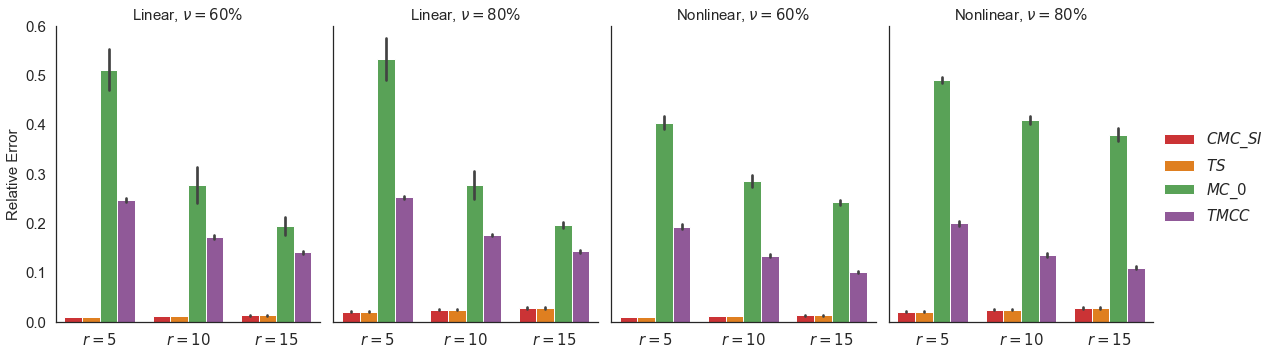
Figure 2: Relative Error of Feature Matrix (with the Black Lines Representing ± the Standard Error)

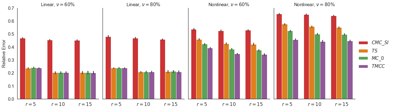
Figure 3: Relative Error of Target Matrix (with the Black Lines Representing ± the Standard Error)

In Fig 2, it is an unsurprising fact that TMCC surpasses MC_0 with the help of calibration information. For instance, in the linear case with $\nu=60\%$, the mean of RE of $\hat{\mathbf{X}}$ by MC_0 is 0.51 with standard error (SE) 0.0417 when $r=5$ while that by TMCC is 0.25 with SE 0.0040. TMCC’s RE is less than half of MC_0’s and situations in other cases are alike. Besides, CMC_SI and TS perform the best in all scenarios. Specifically, the mean of RE of $\hat{\mathbf{X}}$ by CMC_SI is 0.01 with SE 0.0005, and that by TS is 0.01 with SE 0.0006 when $r=10$ in the nonlinear case with $\nu=60\%$. It is because both CMC_SI and TS complete the feature matrix without considering the target matrix. However, our primary goal is to recover $\mathbf{Z}_{\star}$, i.e., achieving a low relative error of $\hat{\mathbf{Z}}$. In Fig 3, the far lower relative error of $\hat{\mathbf{X}}$ by CMC_SI and TS does not bring a lower relative error of $\hat{\mathbf{Z}}$. Of all the four approaches, CMC_SI is the only one that fails to take advantage of the feature matrix to recover the target matrix. That is why it attains the greatest relative error of the target matrix. For example, its mean of RE of $\hat{\mathbf{Z}}$ is 0.46 with SE 0.0046 when $r=15$ in the linear case with $\nu=80\%$ and 0.53 with SE 0.0057 when $r=15$ in the nonlinear case with $\nu=60\%$, more than twice of the other three methods. Besides, TS, MC_0, and TMCC behave similarly in the linear case while they display great differences in the nonlinear case. When the relationship between $\mathbf{X}_{\star}$ and $\mathbf{Z}_{\star}$ is not linear, simultaneously recovering demonstrates great strength compared with recovering step by step and recovering separately. In the nonlinear case with $\nu=80\%$, the means of RE of $\hat{\mathbf{Z}}$ by CMC_SI, TS, MC_0, and TMCC are 0.66, 0.58, 0.52, and 0.46 respectively when $r=5$. Situations in other cases are almost the same. What is noteworthy is that TMCC also overtakes MC_0 with respect to target matrices, which implies the power of calibration information again. Overall, relatively low standard errors indicate the stability of these algorithms.

5 Conclusion

We proposed a statistical framework for multi-task learning under exponential family matrix completion framework with known calibration information. Statistical guarantee of our proposed estimator has been shown and a constant order improvement is achieved compared with existing methods. We have also shown that the proposed algorithm has a convergence rate of $O(1/k^{2})$. The simulation study also shows that our proposed method has numerical benefits.

Appendix

In this appendix, we provide technical proofs and computational time comparisons for our main article. Specifically, it is organized as follows:

• Section A introduces necessary preliminary;

• Section B presents proof of Theorem 1;

• Section C presents proof of Theorem 2;

• Section D provides auxiliary lemmas;

• Section E provides computational time comparison for the simulations.

Appendix A PRELIMINARY

In the following, we investigate the theoretical properties of the proposed TMCC algorithm. Before going through those theoretical results, we first introduce some useful matrix norm inequalities. For two matrices $\mathbf{S}$ and $\mathbf{T}$ with the same dimension, define the inner product in terms of the trace of the matrix product, i.e., $\langle\mathbf{S},\mathbf{T}\rangle=\mbox{tr}(\mathbf{S}^{\rm T}\mathbf{T})$. We have trace duality inequality

$$\left|\mbox{tr}(\mathbf{S}^{\rm T}\mathbf{T})\right|\leq\left\|\mathbf{S}\right\|\left\|\mathbf{T}\right\|_{\star},$$ (A.4)

and bound for nuclear norm

$$\left\|\mathbf{S}\right\|_{\star}\leq\sqrt{\mbox{rank}(\mathbf{S})}\left\|\mathbf{S}\right\|_{F}.$$ (A.5)

Further,

$$\sigma_{\min}(\mathbf{S})\left\|\mathbf{T}\right\|_{F}\leq\left\|\mathbf{S}\mathbf{T}\right\|_{F},$$ (A.6)

where the proof of (A.6) is presented in Lemma 2. Suppose the SVD of $\mathbf{S}$ is $\mathbf{U}_{\mathbf{S}}\Sigma_{\mathbf{S}}\mathbf{V}^{\rm T}_{\mathbf{S}}$. Let $\widetilde{\mathbf{P}}_{\mathbf{S}}=\mathbf{S}(\mathbf{S}^{\rm T}\mathbf{S})^{-1}\mathbf{S}^{\rm T}$ be the projection matrix based on $\mathbf{S}$. Define $\mathcal{P}_{\mathbf{S}}^{\perp}(\mathbf{T})=\widetilde{\mathbf{P}}_{\mathbf{U}_{\mathbf{S}}^{\perp}}\mathbf{T}\widetilde{\mathbf{P}}_{\mathbf{V}_{\mathbf{S}}^{\perp}}$, where $\mathbf{F}^{\perp}=(\mathbf{I}-\widetilde{\mathbf{P}}_{\mathbf{F}})\mathbf{F}$ for a matrix $\mathbf{F}$. Notice that $\mathcal{P}_{\mathbf{S}}^{\perp}(\mathbf{T})$ is not a projection since it is not idempotent. Let $\mathcal{P}_{\mathbf{S}}(\mathbf{T})=\mathbf{T}-\mathcal{P}_{\mathbf{S}}^{\perp}(\mathbf{T})$ and we have

$$\mbox{rank}\left\{\mathcal{P}_{\mathbf{S}}(\mathbf{T})\right\}\leq 2\mbox{rank}(\mathbf{S}).$$ (A.7)

By [24], we have

$$\left\|\mathbf{S}\right\|_{\star}-\left\|\mathbf{T}\right\|_{\star}\leq\left\|\mathcal{P}_{\mathbf{S}}(\mathbf{S}-\mathbf{T})\right\|_{\star}+\left\|\mathcal{P}_{\mathbf{S}}^{\perp}(\mathbf{S}-\mathbf{T})\right\|_{\star}.$$ (A.8)

Finally, we define the Bregman divergence.

Definition 1.

Let $\mathcal{C}$ be a closed set. For a continuously-differentiable function $F:\mathcal{C}\rightarrow\mathbb{R}$, the Bregman divergence associated with $F$ between $x,y\in\mathcal{C}$ is

$$d_{F}(x,y)=F(x)-F(y)-\langle\nabla F(y),x-y\rangle.$$

Mathematically, $d_{F}(x,y)$ is equivalent to the first-order Taylor expansion error of $F(x)$ evaluated at $y$.

Denote $\boldsymbol{\Sigma}_{R}$ to be an $n\times D$ matrix, consisting of $i.i.d.$ Rademacher sequences $\{\xi_{x,ij}:i\in[n],j\in[d]\}$ and $\{\xi_{y,ij}^{(s)}:i\in[n],j\in[m_{s}]\}$ for $s\in[S]$. Specifically,

$$\boldsymbol{\Sigma}_{R}= \sum_{(i,j)}^{(n,d)}\xi_{x,ij}r_{x,ij}\mathbf{E}_{x,ij}+\sum_{s=1}^{S}\sum_{(i,j)}^{(n,m_{s})}\xi_{y,ij}^{(s)}r_{y,ij}^{(s)}\mathbf{E}_{y,ij}^{(s)},$$

where $\mathbf{E}_{x,ij}=\mathbf{e}_{i}(n)\mathbf{e}_{j}(D)^{\rm T}$ and $\mathbf{E}_{y,ij}^{(s)}=\mathbf{e}_{i}(n)\mathbf{e}_{\tilde{j}}(D)^{\rm T}$ are $\mathbb{R}^{n\times D}$ matrices lying in the set of canonical bases, $\mathbf{e}_{i}(l)$ is the $j$-th unit vector of length $l$ and $\tilde{j}=j+d+\sum_{t=1}^{s-1}m_{t}$.

Appendix B PROOF OF THEOREM 1

Proof.

Given two arbitrary matrices $\mathbf{S}$, $\mathbf{T}\in\mathbb{R}^{n\times D}$, we have

$$\left|f_{\tau_{1}}(\mathbf{S})-f_{\tau_{1}}(\mathbf{T})\right|$$

$$= \left|\left\{\tilde{\ell}(\mathbf{S})-\tilde{\ell}(\mathbf{T})\right\}-\tau_{1}\left\{\left\|\mathbf{A}\left(\mathbf{S}-\mathbf{M}_{\star}\right)\right\|_{F}^{2}-\left\|\mathbf{A}\left(\mathbf{T}-\mathbf{M}_{\star}\right)\right\|_{F}^{2}\right\}\right|$$

$$\leq \left|\tilde{\ell}(\mathbf{S})-\tilde{\ell}(\mathbf{T})\right|+\tau_{1}\left|\left\{\left\|\mathbf{A}\left(\mathbf{S}-\mathbf{M}_{\star}\right)\right\|_{F}^{2}-\left\|\mathbf{A}\left(\mathbf{T}-\mathbf{M}_{\star}\right)\right\|_{F}^{2}\right\}\right|$$

$$\leq \left\|\nabla\tilde{\ell}\left(\widetilde{\mathbf{M}}\right)\right\|\left\|\mathbf{S}-\mathbf{T}\right\|_{\star}+\tau_{1}\sigma_{1}^{2}(\mathbf{A})\left\|\mathbf{S}-\mathbf{T}\right\|_{F}\left\|\mathbf{S}+\mathbf{T}-2\mathbf{M}_{\star}\right\|_{F}$$

$$\leq \left\{\sqrt{n\wedge D}\left\|\nabla\tilde{\ell}\left(\widetilde{\mathbf{M}}\right)\right\|+2\tau_{1}\sigma_{1}^{2}(\mathbf{A})\sqrt{nD\alpha}\right\}\left\|\mathbf{S}-\mathbf{T}\right\|_{F},$$

where $\widetilde{\mathbf{M}}\in\mathcal{G}_{\infty}(\alpha)$. We focus on bound of $\|\nabla\tilde{\ell}(\widetilde{\mathbf{M}})\|$.

$$\left\|\nabla\tilde{\ell}\left(\widetilde{\mathbf{M}}\right)\right\|$$

$$\leq \left\|\nabla\tilde{\ell}(\mathbf{M}_{\star})\right\|+\left\|\nabla\tilde{\ell}(\widetilde{\mathbf{M}})-\nabla\tilde{\ell}(\mathbf{M}_{\star})\right\|$$

$$\leq \left\|\nabla\tilde{\ell}(\mathbf{M}_{\star})\right\|+\frac{1}{nD}\left\|\sum_{s=1}^{S}\sum_{(i,j)\in[n]\times[m_{s}]}r_{y,ij}^{(s)}\mathbf{E}_{y,ij}^{(s)}\times\left\{(g^{(s)})^{\prime}(\tilde{z}_{\star,ij}^{(s)})-(g^{(s)})^{\prime}(z_{\star,ij}^{(s)})\right\}\right.$$

$$\left.\quad\quad\quad\quad\quad\quad\quad\quad\quad\quad\quad\quad+\sum_{(i,j)\in[n]\times[d]}r_{x,ij}\mathbf{E}_{x,ij}\left\{g_{N}^{\prime}(\tilde{x}_{ij})-g_{N}^{\prime}(x_{ij})\right\}\right\|$$

$$\leq \left\|\nabla\tilde{\ell}(\mathbf{M}_{\star})\right\|+\frac{\tilde{U}_{\alpha}}{nD}\left\|\sum_{s=1}^{S}\sum_{(i,j)\in[n]\times[m_{s}]}r_{y,ij}^{(s)}\mathbf{E}_{y,ij}^{(s)}\left|\tilde{z}_{\star,ij}^{(s)}-z_{\star,ij}^{(s)}\right|+\sum_{(i,j)\in[n]\times[d]}r_{x,ij}\mathbf{E}_{x,ij}\left|\tilde{x}_{ij}-x_{ij}\right|\right\|$$

$$\leq \frac{c_{2}(\sqrt{\tilde{U}_{\alpha}}\vee 1/\delta)\left[\sqrt{\gamma}+\left\{\log(n\vee D)\right\}^{3/2}\right]}{nD}+\frac{2\sqrt{nD\alpha}\tilde{U}_{\alpha}}{nD}$$

$$\leq \frac{c_{3}}{\sqrt{nD}}.$$

Therefore, as long as $\tau_{1}\leq c_{1}\{\sigma_{1}(\mathbf{A})\}^{-2}(nD\alpha)^{-1/2}$, there exists positive constant $\tilde{L}=2c_{1}+c_{3}$ such that $f_{\tau_{1}}(\cdot)$ is $\tilde{L}$-Lipchitz. The remaining proof can be obtained by followed the proof of Theorem 4.1 in [22]. ∎

Appendix C PROOF OF THEOREM 2

Proof.

In general, we use the connection between exponential family distributions and Bregman divergence to argue the basic inequality implied by our estimation procedure. Then, a key quantity can be bounded and the results can be obtained by the standard argument for matrix completion. Specifically, by basic inequality, we have

$$\frac{1}{nD}\left[\sum_{s=1}^{S}\sum_{(i,j)\in[n]\times[m_{s}]}r_{y,ij}^{(s)}\left\{-y_{ij}^{(s)}\hat{z}_{ij}^{(s)}+g^{(s)}(\hat{z}_{ij}^{(s)})\right\}+\sum_{(i,j)\in[n]\times[d]}\frac{r_{x,ij}}{2}(\hat{x}_{ij}-x_{ij})^{2}\right]$$

$$\quad\quad+\tau_{1}\left\|\mathbf{A}\widehat{\mathbf{X}}-\mathbf{B}\right\|_{F}^{2}+\tau_{2}\left\|\widehat{\mathbf{M}}\right\|_{\star}$$

$$\leq \frac{1}{nD}\left[\sum_{s=1}^{S}\sum_{(i,j)\in[n]\times[m_{s}]}r_{y,ij}^{(s)}\left\{-y_{ij}^{(s)}z_{\star,ij}+g^{(s)}(z_{\star,ij}^{(s)})\right\}+\sum_{(i,j)\in[n]\times[d]}\frac{r_{x,ij}}{2}(x_{\star,ij}-x_{ij})^{2}\right]$$

$$\quad\quad+\tau_{1}\left\|\mathbf{A}\mathbf{X}_{\star}-\mathbf{B}\right\|_{F}^{2}+\tau_{2}\left\|\mathbf{M}_{\star}\right\|_{\star}$$

$$= \frac{1}{nD}\left[\sum_{s=1}^{S}\sum_{(i,j)\in[n]\times[m_{s}]}r_{y,ij}^{(s)}\left\{-y_{ij}^{(s)}z_{\star,ij}+g^{(s)}(z_{\star,ij}^{(s)})\right\}+\sum_{(i,j)\in[n]\times[d]}\frac{r_{x,ij}}{2}(x_{\star,ij}-x_{ij})^{2}\right]+\tau_{2}\left\|\mathbf{M}_{\star}\right\|_{\star},$$

where the calibration information implies the last equality. Let $g_{N}(x)=x^{2}/2$, expanding quadratic terms of $x_{ij}$, and we have

$$\frac{1}{nD}\left[\sum_{s=1}^{S}\sum_{(i,j)\in[n]\times[m_{s}]}r_{y,ij}^{(s)}\left\{-y_{ij}^{(s)}\hat{z}_{ij}^{(s)}+g^{(s)}(\hat{z}_{ij}^{(s)})\right\}+\sum_{(i,j)\in[n]\times[d]}r_{x,ij}\left\{-x_{ij}\hat{x}_{ij}+g_{N}(\hat{x}_{ij})\right\}\right]$$

$$\quad\quad+\tau_{1}\left\|\mathbf{A}\widehat{\mathbf{X}}-\mathbf{B}\right\|_{F}^{2}+\tau_{2}\left\|\widehat{\mathbf{M}}\right\|_{\star}$$

$$\leq \frac{1}{nD}\left[\sum_{s=1}^{S}\sum_{(i,j)\in[n]\times[m_{s}]}r_{y,ij}^{(s)}\left\{-y_{ij}^{(s)}z_{\star,ij}+g^{(s)}(z_{\star,ij}^{(s)})\right\}+\sum_{(i,j)\in[n]\times[d]}r_{x,ij}\left\{-x_{ij}{x}_{\star,ij}+g_{N}(x_{\star,ij})\right\}\right]+\tau_{2}\left\|\mathbf{M}_{\star}\right\|_{\star}.$$

Rearranging the terms, we obtain

$$\frac{1}{nD}\left(\sum_{s=1}^{S}\sum_{(i,j)\in[n]\times[m_{s}]}r_{y,ij}^{(s)}\left[-y_{ij}^{(s)}\left(\widehat{z}_{ij}^{(s)}-z_{\star,ij}^{(s)}\right)+\left\{g^{(s)}(\widehat{z}_{ij}^{(s)})-g^{(s)}(z_{\star,ij}^{(s)})\right\}\right]+\right.$$

$$\left.\quad\sum_{(i,j)\in[n]\times[d]}r_{x,ij}\times\left[-x_{ij}(\hat{x}_{ij}-x_{\star,ij})+\left\{g_{N}(\hat{x}_{ij})-g_{N}(x_{\star,ij})\right\}\right]\right)$$

$$\leq -\tau_{1}\left\|\mathbf{A}\widehat{\mathbf{X}}-\mathbf{B}\right\|_{F}^{2}+\tau_{2}\left(\left\|\mathbf{M}_{\star}\right\|_{\star}-\left\|\widehat{\mathbf{M}}\right\|_{\star}\right)$$

$$= -\tau_{1}\left\|\mathbf{A}\left(\widehat{\mathbf{X}}-\mathbf{X}_{\star}\right)\right\|_{F}^{2}+\tau_{2}\left(\left\|\mathbf{M}_{\star}\right\|_{\star}-\left\|\widehat{\mathbf{M}}\right\|_{\star}\right).$$ (C.9)

Plug in the Bregman divergence into (C) with (A.4), and we have

$$\frac{1}{nD}\left[\sum_{s=1}^{S}\sum_{(i,j)\in[n]\times[m_{s}]}\left\{r_{y,ij}^{(s)}d_{g^{(s)}}\left(\widehat{z}_{ij}^{(s)},z_{\star,ij}^{(s)}\right)\right\}+\sum_{(i,j)\in[n]\times[d]}\left\{r_{x,ij}^{(s)}d_{g_{N}}\left(\widehat{x}_{ij},x_{\star,ij}\right)\right\}\right]$$

$$\leq -\tau_{1}\left\|\mathbf{A}\widehat{\mathbf{X}}-\mathbf{B}\right\|_{F}^{2}+\tau_{2}\left(\left\|\mathbf{M}_{\star}\right\|_{\star}-\left\|\widehat{\mathbf{M}}\right\|_{\star}\right)-$$

$$\quad\frac{1}{nD}\left[\sum_{s=1}^{S}\sum_{(i,j)\in[n]\times[m_{s}]}r_{y,ij}^{(s)}\times\quad\left\{\left(g^{(s)}\right)^{\prime}(z_{\star,ij}^{(s)})-y_{ij}^{(s)}\right\}\left(\widehat{z}_{ij}^{(s)}-z_{\star,ij}^{(s)}\right)+\right.$$

$$\left.\quad\quad\quad\sum_{(i,j)\in[n]\times[d]}r_{x,ij}\left\{(g_{N})^{\prime}(x_{\star,ij})-x_{ij}\right\}(\hat{x}_{ij}-x_{\star,ij})\right]$$

$$= -\tau_{1}\left\|\mathbf{A}\widehat{\mathbf{X}}-\mathbf{B}\right\|_{F}^{2}+\tau_{2}\left(\left\|\mathbf{M}_{\star}\right\|_{\star}-\left\|\widehat{\mathbf{M}}\right\|_{\star}\right)-\langle\nabla\tilde{\ell}(\mathbf{M}_{\star}),\widehat{\mathbf{M}}-\mathbf{M}_{\star}\rangle$$

$$\leq -\tau_{1}\left\|\mathbf{A}\widehat{\mathbf{X}}-\mathbf{B}\right\|_{F}^{2}+\tau_{2}\left(\left\|\mathbf{M}_{\star}\right\|_{\star}-\left\|\widehat{\mathbf{M}}\right\|_{\star}\right)+\left\|\nabla\tilde{\ell}(\mathbf{M}_{\star})\right\|\left\|\widehat{\mathbf{M}}-\mathbf{M}_{\star}\right\|_{\star},$$ (C.10)

where $\tilde{\ell}(\mathbf{M}_{\star})=(nD)^{-1}[\ell(\mathbf{Z}_{\star})+\sum_{(i,j)\in[n]\times[d]}r_{x,ij}\times\{-x_{ij}x_{\star,ij}+g_{N}(x_{\star,ij})\}]$. With an additional assumption that $\tau_{2}\geq 2\|\nabla\tilde{\ell}(\mathbf{M}_{\star})\|$, together with (A.5) and (A.7), (C) yields

$$\frac{1}{nD}\left\{\sum_{s=1}^{S}\sum_{(i,j)\in[n]\times[m_{s}]}r_{y,ij}^{(s)}d_{g^{(s)}}\left(\widehat{z}_{ij}^{(s)},z_{\star,ij}^{(s)}\right)+\sum_{(i,j)\in[n]\times[d]}r_{x,ij}d_{g_{N}}(\hat{x}_{ij},x_{\star,ij})\right\}$$

$$\leq \frac{3\tau_{2}}{2}\left\|\mathcal{P}_{\mathbf{M}}\left(\widehat{\mathbf{M}}-\mathbf{M}_{\star}\right)\right\|_{\star}-\tau_{1}\left\|\mathbf{A}\left(\widehat{\mathbf{X}}-\mathbf{X}_{\star}\right)\right\|_{F}^{2}$$

$$\leq \frac{3\tau_{2}}{2}\sqrt{2\mbox{rank}(\mathbf{M}_{\star})}\left\|\widehat{\mathbf{M}}-\mathbf{M}_{\star}\right\|_{F}-\tau_{1}\left\|\mathbf{A}\left(\widehat{\mathbf{X}}-\mathbf{X}_{\star}\right)\right\|_{F}^{2}.$$ (C.11)

Meanwhile, as $L_{\alpha}(x-y)^{2}\leq 2d_{g^{(s)}}(x,y)\leq U_{\alpha}(x-y)^{2}$ and $2d_{g_{N}}(x,y)=(x-y)^{2}$, we have

$$\Delta_{\tilde{\ell}}^{2}\leq \frac{2}{\tilde{L}_{\alpha}nD}\left\{\sum_{s=1}^{S}\sum_{(i,j)\in[n]\times[m_{s}]}r_{y,ij}^{(s)}d_{g^{(s)}}\left(\widehat{z}_{ij}^{(s)},z_{\star,ij}^{(s)}\right)+\sum_{(i,j)\in[n]\times[d]}r_{x,ij}d_{g_{N}}(\hat{x}_{ij},x_{\star,ij})\right\},$$

where

$$\Delta_{\tilde{\ell}}^{2}= \frac{1}{nD}\left\{\sum_{s=1}^{S}\sum_{(i,j)\in[n]\times[m_{s}]}r_{y,ij}^{(s)}\left(\widehat{z}_{ij}^{(s)}-z_{\star,ij}^{(s)}\right)^{2}+\sum_{(i,j)\in[n]\times[d]}r_{x,ij}\left(\hat{x}_{ij}-x_{\star,ij}\right)^{2}\right\}.$$ (C.12)

Put (C) and (C.12) together, and we obtain

$$\Delta_{\tilde{\ell}}^{2}\leq \frac{2}{\tilde{L}_{\alpha}}\left\{\frac{3\tau_{2}}{2}\sqrt{2\mbox{rank}(\mathbf{M}_{\star})}\left\|\widehat{\mathbf{M}}-\mathbf{M}_{\star}\right\|_{F}-\tau_{1}\left\|\mathbf{A}\left(\widehat{\mathbf{X}}-\mathbf{X}_{\star}\right)\right\|_{F}^{2}\right\}.$$ (C.13)

With Lemma 1 and 5 in the Appendix, follow the proof of Theorem 3 in [7], our main theorem is proved.

∎

Appendix D AUXILIARY LEMMAS

Lemma 1.

Let arbitrary matrices $\mathbf{S},\mathbf{T}\in\mathcal{G}_{\infty}(\alpha)$. Assume that $\tau_{2}\geq 2\|\nabla\tilde{\ell}(\mathbf{T})\|$ and $\tilde{\ell}(\mathbf{S})+\tau_{2}\|\mathbf{S}\|_{\star}\leq\tilde{\ell}(\mathbf{T})-\tau_{1}\|\mathbf{A}(\mathbf{S}_{[d]}-\mathbf{T}_{[d]})\|_{F}^{2}+\tau_{2}\|\mathbf{T}\|_{\star}$, where $\mathbf{S}_{[d]}$ consists of the first $d$ columns of $\mathbf{S}$. Then we have

1. $\left\|\mathcal{P}_{\mathbf{T}}^{\perp}(\mathbf{S}-\mathbf{T})\right\|_{\star}\leq 3\left\|\mathcal{P}_{\mathbf{T}}(\mathbf{S}-\mathbf{T})\right\|_{F}-2\tau_{1}\tau_{2}^{-1}\sigma_{\min}^{2}(\mathbf{A})\left\|\mathbf{S}_{[d]}-\mathbf{T}_{[d]}\right\|_{F}^{2}$,

2. $\left\|\mathbf{S}-\mathbf{T}\right\|_{\star}\leq 4\sqrt{2\mbox{rank}(\mathbf{T})}\left\|\mathbf{S}-\mathbf{T}\right\|_{F}-2\tau_{1}\tau_{2}^{-1}\sigma_{\min}^{2}(\mathbf{A})\left\|\mathbf{S}_{[d]}-\mathbf{T}_{[d]}\right\|_{F}^{2}$.

Proof.

Rearranging the terms, we have

$$\tau_{2}\left(\left\|\mathbf{S}\right\|_{\star}-\left\|\mathbf{T}\right\|_{\star}\right)\leq\tilde{\ell}(\mathbf{T})-\tilde{\ell}(\mathbf{S})-\tau_{1}\left\|\mathbf{A}(\mathbf{S}_{[d]}-\mathbf{T}_{[d]})\right\|_{F}^{2}.$$ (D.14)

By convexity of $\tilde{\ell}(\cdot)$ and (A.4), we have

$$\tilde{\ell}(\mathbf{T})-\tilde{\ell}(\mathbf{S})\leq\langle\nabla\tilde{\ell}(\mathbf{T}),\mathbf{T}-\mathbf{S}\rangle\leq\left\|\nabla\tilde{\ell}(\mathbf{T})\right\|\left\|\mathbf{T}-\mathbf{S}\right\|_{\star}\leq\frac{\tau_{2}}{2}\left\|\mathbf{T}-\mathbf{S}\right\|_{\star}.$$ (D.15)

Plug (D.15) in (D.14) with (A.8), and we obtain

$$\tau_{2}\left\|\mathcal{P}_{\mathbf{T}}^{\perp}(\mathbf{S}-\mathbf{T})\right\|_{\star}-\tau_{2}\left\|\mathcal{P}_{\mathbf{T}}(\mathbf{S}-\mathbf{T})\right\|_{\star}\leq\frac{\tau_{2}}{2}\left\|\mathbf{T}-\mathbf{S}\right\|_{\star}-\tau_{1}\left\|\mathbf{A}(\mathbf{S}_{[d]}-\mathbf{T}_{[d]})\right\|_{F}^{2}.$$

Rearranging terms, we have

$$\left\|\mathcal{P}_{\mathbf{T}}^{\perp}(\mathbf{S}-\mathbf{T})\right\|_{\star}$$

$$\leq 3\left\|\mathcal{P}_{\mathbf{T}}(\mathbf{S}-\mathbf{T})\right\|_{\star}-\frac{2\tau_{1}}{\tau_{2}}\left\|\mathbf{A}(\mathbf{S}_{[d]}-\mathbf{T}_{[d]})\right\|_{F}^{2}$$

$$\leq 3\left\|\mathcal{P}_{\mathbf{T}}(\mathbf{S}-\mathbf{T})\right\|_{\star}-\frac{2\tau_{1}}{\tau_{2}}\sigma_{\min}^{2}(\mathbf{A})\left\|(\mathbf{S}_{[d]}-\mathbf{T}_{[d]})\right\|_{F}^{2},$$

where the first part is proved. For the second part, we have

$$\left\|\mathbf{S}-\mathbf{T}\right\|_{\star}$$

$$= \left\|\mathcal{P}_{\mathbf{T}}^{\perp}(\mathbf{S}-\mathbf{T})+\mathcal{P}_{\mathbf{T}}(\mathbf{S}-\mathbf{T})\right\|_{\star}$$

$$\leq \left\|\mathcal{P}_{\mathbf{T}}^{\perp}(\mathbf{S}-\mathbf{T})\right\|_{\star}+\left\|\mathcal{P}_{\mathbf{T}}(\mathbf{S}-\mathbf{T})\right\|_{\star}$$

$$\leq 4\left\|\mathcal{P}_{\mathbf{T}}(\mathbf{S}-\mathbf{T})\right\|_{\star}-\frac{2\tau_{1}}{\tau_{2}}\sigma_{\min}^{2}(\mathbf{A})\left\|(\mathbf{S}_{[d]}-\mathbf{T}_{[d]})\right\|_{F}^{2}$$

$$\leq 4\sqrt{2\mbox{rank}(\mathbf{T})}\left\|\mathbf{S}-\mathbf{T}\right\|_{F}-\frac{2\tau_{1}}{\tau_{2}}\sigma_{\min}^{2}(\mathbf{A})\left\|\mathbf{S}_{[d]}-\mathbf{T}_{[d]}\right\|_{F}^{2}.$$

∎

Lemma 2.

Given $\mathbf{S}$ and $\mathbf{T}$ of arbitrary matrices with the same dimension,

$$\sigma_{\min}(\mathbf{S})\left\|\mathbf{T}\right\|_{F}\leq\left\|\mathbf{S}\mathbf{T}\right\|_{F}.$$

Proof.

By singular value decomposition, let $\mathbf{S}=\mathbf{U}_{\mathbf{S}}\Lambda_{\mathbf{S}}\mathbf{V}_{\mathbf{S}}^{\rm T}$ and $\mathbf{T}=\mathbf{U}_{\mathbf{T}}\Lambda_{\mathbf{T}}\mathbf{V}_{\mathbf{T}}^{\rm T}$. Then by the cyclic property of trace operator,

$$\left\|\mathbf{S}\mathbf{T}\right\|_{F}^{2} =\left\|\mathbf{U}_{\mathbf{S}}\Sigma_{\mathbf{S}}\mathbf{V}_{\mathbf{S}}^{\rm T}\mathbf{U}_{\mathbf{T}}\Sigma_{\mathbf{T}}\mathbf{V}_{\mathbf{T}}^{\rm T}\right\|_{F}^{2}$$

$$=\mbox{tr}\left(\mathbf{V}_{\mathbf{T}}\Sigma_{\mathbf{T}}\mathbf{U}_{\mathbf{T}}^{\rm T}\mathbf{V}_{\mathbf{S}}\Sigma_{\mathbf{S}}\mathbf{U}_{\mathbf{S}}^{\rm T}\mathbf{U}_{\mathbf{S}}\Sigma_{\mathbf{S}}\mathbf{V}_{\mathbf{S}}^{\rm T}\mathbf{U}_{\mathbf{T}}\Sigma_{\mathbf{T}}\mathbf{V}_{\mathbf{T}}^{\rm T}\right)$$

$$=\mbox{tr}\left(\mathbf{V}_{\mathbf{S}}\Sigma_{\mathbf{S}}^{2}\mathbf{V}_{\mathbf{S}}^{\rm T}\mathbf{U}_{\mathbf{T}}\Sigma_{\mathbf{T}}\mathbf{V}_{\mathbf{T}}^{\rm T}\mathbf{V}_{\mathbf{T}}\Sigma_{\mathbf{T}}\mathbf{U}_{\mathbf{T}}^{\rm T}\right)$$

$$\geq\sigma_{\min}^{2}(\mathbf{S})\mbox{Tr}\left(\mathbf{U}_{\mathbf{T}}\Sigma_{\mathbf{T}}\mathbf{V}_{\mathbf{T}}^{\rm T}\mathbf{V}_{\mathbf{T}}\Sigma_{\mathbf{T}}\mathbf{U}_{\mathbf{T}}^{\rm T}\right)$$

$$=\sigma_{\min}^{2}(\mathbf{S})\left\|\mathbf{T}\right\|_{F}^{2}.$$

∎

The following three lemmas can be adapted from [7].

Lemma 3 (Modified Lemma 5 of [7]).

Suppose that Assumption 1 holds. There exists a positive constant $c$, such that

$$\mathbb{E}\left(\left\|\boldsymbol{\Sigma}_{R}\right\|\right)\leq\frac{c\left\{\sqrt{\gamma}+\sqrt{\log{(n\vee D)}}\right\}}{nD}.$$

Lemma 4 (Modified Lemma 6 of [7]).

Suppose that Assumption 1, 3 and 4 hold and there exists a positive constant $c$, such that

$$\left\|\nabla\tilde{\ell}(\mathbf{M}_{\star})\right\|\leq\frac{c(\sqrt{\tilde{U}_{\alpha}}\vee 1/\delta)\left[\sqrt{\gamma}+\left\{\log(n\vee D)\right\}^{3/2}\right]}{nD}$$

holds with probability at least $1-4/(n+D)$.

Lemma 5 (Modified Lemma 19 of [7]).

Suppose that Assumption $1\sim 3$ hold. Let $\beta=946(p_{\min}nD)^{-1}\alpha^{2}\log(n+D)$. Let

$$\mathcal{H}(\mathbf{M}_{\star},\alpha,\beta,\mu,\theta)= \left\{\mathbf{H}\in\mathcal{G}_{\infty}(\alpha):\left\|\mathbf{H}-\mathbf{M}_{\star}\right\|_{\star}\leq\sqrt{\mu}\left\|\mathbf{H}-\mathbf{M}_{\star}\right\|_{F}-\theta\left\|\mathbf{H}_{[d]}-\mathbf{M}_{\star[d]}\right\|_{F}^{2},\right.$$

$$\left.\quad\quad\frac{1}{nD}\left\|\widehat{\mathbf{M}}-\mathbf{M}_{\star}\right\|_{\Pi,F}^{2}>\beta\right\}.$$

Then, for any $\mathbf{H}\in\mathcal{H}(\mathbf{M}_{\star},\alpha,\beta,\mu,\theta)$,

$$\left|\Delta_{\tilde{\ell}}(\mathbf{H},\mathbf{M}_{\star})-\frac{1}{nD}\left\|\mathbf{H}-\mathbf{M}_{\star}\right\|_{\Pi,F}^{2}\right|\leq\frac{1}{2nD}\left\|\mathbf{H}-\mathbf{M}_{\star}\right\|_{\Pi,F}^{2}+\frac{1392nD\alpha^{2}\mu}{p_{\min}}\left\{\mathbb{E}(\left\|\boldsymbol{\Sigma}_{R}\right\|)\right\}^{2}+\frac{5567\alpha^{2}}{nDp_{\min}},$$

with probability at least $1-4(n+D)^{-1}$.

Appendix E Computational Time Comparison

In terms of accuracy, our algorithm outperforms others. For the computational time, our algorithm enjoys a sublinear rate, which is the same as the CMS_SI method. Besides, TS and MC_0 methods are just small deviations from TMCC method, and they enjoy the same sublinear convergence rate. We present the computational behavior among different methods under the missing rate $\nu=80\%$, rank $r$ = 15 with $50$ trials. Further, the stopping criterion for the objective is $\kappa=1e-7$. For TS, the first stage (Feature matrix recovery) stopping criterion is $\kappa_{0}=1e-12$. The results are presented in Table 1, where the running time for TS consists of the time for the first stage plus that for the second stage. The results show the comparable elapsed time for the four methods.

Table 1: Computational Time for Different Scenarios.

Transformation Measure CMC_SI TS MC_0 TMCC Linear Average Time(s) 569.82 1865.40 (185.19+1680.21) 676.20 926.53 Standard Error 78.19 801.61 (107.40+753.79) 50.86 125.39 Nonlinear Average Time(s) 271.78 1072.69 (201.79+870.90) 1141.88 1108.50 Standard Error 28.13 323.55 (110.12+255.70) 476.88 247.77

References

- [1] Rich Caruana, “Multitask learning,” Machine Learning, vol. 28, no. 1, pp. 41–75, 1997.
- [2] Benjamin Recht, “A simpler approach to matrix completion,” Journal of Machine Learning Research, vol. 12, no. Dec, pp. 3413–3430, 2011.
- [3] Raghunandan Keshavan, Andrea Montanari, and Sewoong Oh, “Matrix completion from noisy entries,” Advances in neural information processing systems, vol. 22, 2009.
- [4] Vladimir Koltchinskii, Karim Lounici, and Alexandre B Tsybakov, “Nuclear-norm penalization and optimal rates for noisy low-rank matrix completion,” The Annals of Statistics, vol. 39, no. 5, pp. 2302–2329, 2011.
- [5] Sahand Negahban and Martin J Wainwright, “Restricted strong convexity and weighted matrix completion: Optimal bounds with noise,” Journal of Machine Learning Research, vol. 13, no. May, pp. 1665–1697, 2012.
- [6] Tony Cai and Wen-Xin Zhou, “A max-norm constrained minimization approach to 1-bit matrix completion,” Journal of Machine Learning Research, vol. 14, no. 1, pp. 3619–3647, 2013.
- [7] Mokhtar Z Alaya and Olga Klopp, “Collective matrix completion,” Journal of Machine Learning Research, vol. 20, no. 148, pp. 1–43, 2019.
- [8] Jianqing Fan, Wenyan Gong, and Ziwei Zhu, “Generalized high-dimensional trace regression via nuclear norm regularization,” Journal of Econometrics, vol. 212, no. 1, pp. 177–202, 2019.
- [9] Geneviève Robin, Olga Klopp, Julie Josse, Éric Moulines, and Robert Tibshirani, “Main effects and interactions in mixed and incomplete data frames,” Journal of the American Statistical Association, vol. 115, no. 531, pp. 1292–1303, 2020.
- [10] Andrew Goldberg, Ben Recht, Junming Xu, Robert Nowak, and Jerry Zhu, “Transduction with matrix completion: Three birds with one stone,” in Advances in neural information processing systems, 2010, pp. 757–765.
- [11] Miao Xu, Gang Niu, Bo Han, Ivor W Tsang, Zhi-Hua Zhou, and Masashi Sugiyama, “Matrix co-completion for multi-label classification with missing features and labels,” arXiv preprint arXiv:1805.09156, 2018.
- [12] Ashkan Esmaeili, Kayhan Behdin, Mohammad Amin Fakharian, and Farokh Marvasti, “Transduction with matrix completion using smoothed rank function,” arXiv preprint arXiv:1805.07561, 2018.
- [13] Kai-Yang Chiang, Inderjit S Dhillon, and Cho-Jui Hsieh, “Using side information to reliably learn low-rank matrices from missing and corrupted observations,” Journal of Machine Learning Research, vol. 19, no. 1, pp. 3005–3039, 2018.
- [14] Jean-Claude Deville and Carl-Erik Särndal, “Calibration estimators in survey sampling,” Journal of the American Statistical Association, vol. 87, no. 418, pp. 376–382, 1992.
- [15] Carl-Erik Särndal, Bengt Swensson, and Jan Wretman, Model assisted survey sampling, Springer Science & Business Media, 2003.
- [16] Wayne A Fuller, Sampling statistics, John Wiley & Sons, 2011.
- [17] F Jay Breidt and Jean D Opsomer, “Local polynomial regresssion estimators in survey sampling,” The Annals of Statistics, vol. 28, no. 4, pp. 1026–1053, 2000.
- [18] Changbao Wu and Randy R Sitter, “A model-calibration approach to using complete auxiliary information from survey data,” Journal of the American Statistical Association, vol. 96, no. 453, pp. 185–193, 2001.
- [19] Jae Kwang Kim and Mingue Park, “Calibration estimation in survey sampling,” International Statistical Review, vol. 78, no. 1, pp. 21–39, 2010.
- [20] James Bennett and Stan Lanning, “The netflix prize,” in Proceedings of KDD cup and workshop. Citeseer, 2007, vol. 2007, p. 35.
- [21] Jian-Feng Cai, Emmanuel J Candès, and Zuowei Shen, “A singular value thresholding algorithm for matrix completion,” SIAM Journal on Optimization, vol. 20, no. 4, pp. 1956–1982, 2010.
- [22] Shuiwang Ji and Jieping Ye, “An accelerated gradient method for trace norm minimization,” in Proceedings of the 26th annual international conference on machine learning, 2009, pp. 457–464.
- [23] Rahul Mazumder, Trevor Hastie, and Robert Tibshirani, “Spectral regularization algorithms for learning large incomplete matrices,” Journal of Machine Learning Research, vol. 11, no. Aug, pp. 2287–2322, 2010.
- [24] Olga Klopp, “Noisy low-rank matrix completion with general sampling distribution,” Bernoulli, vol. 20, no. 1, pp. 282–303, 2014.