Escaping limit cycles: Global convergence for constrained nonconvex-nonconcave minimax problems

Abstract

This paper introduces a new extragradient-type algorithm for a class of nonconvex-nonconcave minimax problems. It is well-known that finding a local solution for general minimax problems is computationally intractable. This observation has recently motivated the study of structures sufficient for convergence of first order methods in the more general setting of variational inequalities when the so-called weak Minty variational inequality (MVI) holds. This problem class captures non-trivial structures as we demonstrate with examples, for which a large family of existing algorithms provably converge to limit cycles. Our results require a less restrictive parameter range in the weak MVI compared to what is previously known, thus extending the applicability of our scheme. The proposed algorithm is applicable to constrained and regularized problems, and involves an adaptive stepsize allowing for potentially larger stepsizes. Our scheme also converges globally even in settings where the underlying operator exhibits limit cycles.

1 Introduction

Many machine learning applications, from generative adversarial networks (GANs) to robust reinforcement learning, result in nonconvex-nonconcave constrained minimax problems, which pose notorious difficulties to the scalable first order methods. Indeed, there is no shortage of results illustrating divergent or cycling behavior when going beyond minimization problems (Benaım & Hirsch, 1999; Hommes & Ochea, 2012; Mertikopoulos et al., 2018b; Hsieh et al., 2021).

Traditionally, minimax problems have been studied for more than half a century under the umbrella of the variational inequalities (VIs). The extragradient-type algorithms from the VI literature was recently brought to the awareness of the machine learning community (Mertikopoulos et al., 2018a; Gidel et al., 2018; Böhm et al., 2020), and have provided a principled way of stabilizing training and avoiding Poincaré recursions. However, these results mostly concern the convex-concave setting.

In nonconvex-nonconcave minimax problems, or more generally nonmonotone variational inequalities (VIs), even finding a local solution is in general intractable. This has been made precise through exponential lower bound of the classical optimization type (Hirsch & Vavasis, 1987) and computational complexity results (Papadimitriou, 1994; Daskalakis et al., 2021b). This is in sharp contrast to minimization problems, where only finding a global solution is intractable. The recent result of (Hsieh et al., 2021) provides some intuition behind this difference by showing that the asymptotic limits of most schemes, including extragradient, can converge to attracting limit cycles.

To make progress in lieu of these negative results, Diakonikolas et al. (2021) proposes a simple generalization of extragradient, called (EG+), that can converge to a stationary point even for a class of nonmonotone problems provided that the weak Minty variational inequality (MVI) holds. This problem class is parametrized by a constant $\rho$, which controls the degree of nonconvexity. However, given the range of $\rho$ in Diakonikolas et al. (2021), the new class is still too small to include even the simplest counterexample of Hsieh et al. (2021) for the general Robbins-Monro schemes.

Contributions

Building on the analysis in Diakonikolas et al. (2021), we propose a new adaptive scheme, called (CurvatureEG+), that converges even in the difficult counter example of Hsieh et al. (2021) as illustrated in Fig. 1. Our main contributions are summarized below.

1. We propose an adaptive extragradient-type algorithm that converges for a larger range of $\rho$, the parameter in the weak MVI assumption (cf. Item 3) than previously known.

2. More importantly, we show that convergence is ensured if $2\rho+\gamma_{k}>0$, where $\gamma_{k}$ is the extrapolation stepsize. This is crucial since by selecting $\gamma_{k}$ through a backtracking procedure larger stepsizes are allowed, which in turn implies convergence for more negative values of $\rho$, thus capturing a larger class of problems. In addition, we show that the linesearch eventually passes without triggering any backtrack if initialized based on the Jacobian of $F$ (cf. Section 4).

3. We present a non-adaptive variant of our algorithm (CEG+), and show that for particular parameter choices (EG+) of Diakonikolas et al. (2021), and when $\rho=0$ the celebrated forward-backward-forward (FBF) algorithm of Tseng (2000) are recovered, thus unifying and generalizing both methods. We improve upon Diakonikolas et al. (2021) by not only relaxing the problem class but also the stepsize range. We show that our results are tight by providing a matching lower bound, thus providing a complete picture of (EG+) under weak MVI.

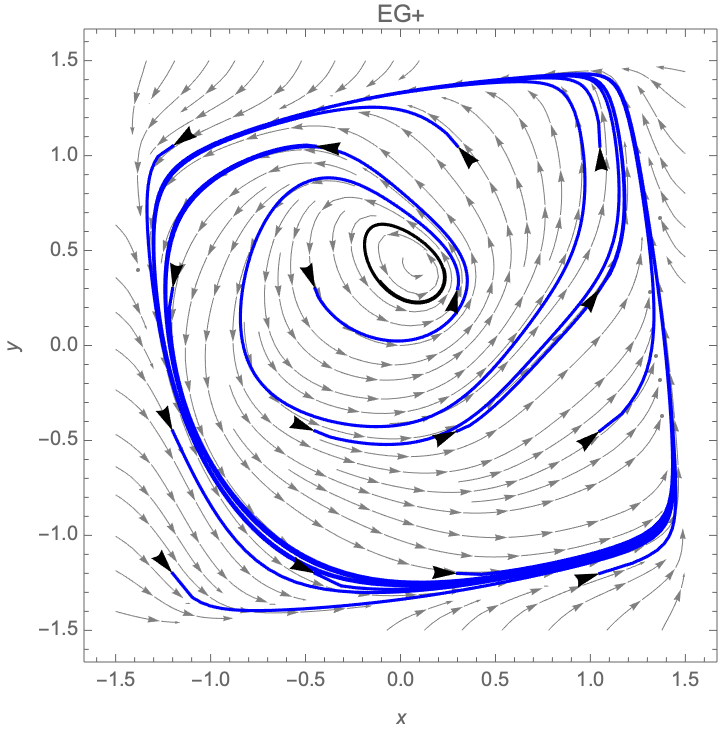
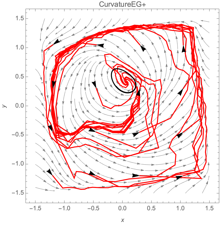
Figure 1: Forsaken (Hsieh et al., 2021, Example 5.2) provides an example where the weak MVI constant $\rho$ does not satisfy algorithmic requirements of (EG+) and (EG+) does not converge to a stationary point but rather the attracting limit cycle (left). In contrast, adaptively choosing the extrapolation stepsize large enough with our new method, called (CurvatureEG+), is sufficient for avoiding the limit cycles (right). The repellant limit cycle is indicated in black and the stream plot shows the vectorfield $Fz$. The blue and red curves indicate multiple trajectories of the algorithms starting from initializations indicated in black. See Section C.4 for properties of Forsaken.

Related work

The community has resorted to various approaches to make progress for nonconvex-nonconcave minimax problems. One line of work focuses on deriving local convergence results (Mazumdar et al., 2019; Fiez & Ratliff, 2020; Heusel et al., 2017). For global results, the two primary approaches have been to either assume a global oracle for the inner problem (Jin et al., 2019; Davis & Drusvyatskiy, 2018) or assume particular problem structure such as the Polyak-Łojasiewicz condition (Nouiehed et al., 2019; Yang et al., 2020) or concavity for the inner problem (Rafique et al., 2019).

We follow the same tradition of assuming structure, but from the general perspective of operator theory. The idea of studying minimax and related problems through the lens of variational inequality has a long history (Minty, 1962; Rockafellar, 1976; Polyak, 1987; Bertsekas, 1997), with recent renewed interest due to its relevance for minimax formulations (Mertikopoulos et al., 2018a; Gidel et al., 2018; Azizian et al., 2020).

One relaxation of the monotone case for which we have positive results is that of Minty variational inequalities (MVI) (Mertikopoulos et al., 2018a; Song et al., 2021; Zhou et al., 2017; Liu et al., 2021), which includes all quasiconvex-concave and starconvex-concave problems. Diakonikolas et al. (2021) introduced the relaxed condition of weak MVI. In the unconstrained setting they showed non-asymptotic convergence results under a restricted problem constant $\rho$. Similarly to us, Lee & Kim (2021a) extends the regime but under the stronger condition of cohypomonotonicity. They do so by studying a more evolved variant of extragradient building on anchoring techniques. We instead directly improve upon (EG+) and generalize it to new settings.

In the stochastic setting, usually the stepsize for the extrapolation step is diminishing. This is the case in Böhm et al. (2020) where they consider a forward-backward-forward type scheme. However, they remain in the monotone setting, where the limit cycles are non-attracting, as exemplified by a bilinear game. Hsieh et al. (2021) recently showed that a large family of algorithms, which includes the extragradient method with diminishing stepsize, can converge to attracting limit cycles. Going beyond this restriction, prior to Diakonikolas et al. (2021), Hsieh et al. (2020) interestingly considers two separate and diminishing stepsizes under the stronger assumption of MVI.

2 Problem formulation and preliminaries

In this paper we are interested in finding zeros of an operator (or set-valued mapping) $T:\mathbb{R}^{n}\rightrightarrows\mathbb{R}^{n}$ that is written as the sum of a Lipschitz continuous (but possibly nonmonotone) operator $F$ and a maximally monotone operator $A$. That is, we wish to find $z\in\mathbb{R}^{n}$ such that the general inclusion

$$0\in Tz\coloneqq Az+Fz$$ (2.1)

holds. The set of all such points is denoted by $\operatorname*{zer}T\coloneqq{\mathopen{}\left\{z\in R^{n}{}\mid{}0\in Tz\right\}\mathclose{}}$. Throughout the paper problem (2.1) is studied under the following assumptions (definitions can be found in Appendix A).

Assumption I.

In problem (2.1),

1. Operator $A:\mathbb{R}^{n}\rightrightarrows\mathbb{R}^{n}$ is a maximally monotone operator.

2. Operator $F:\mathbb{R}^{n}\to\mathbb{R}^{n}$ is $L$-Lipschitz continuous.

3. Weak Minty variational inequality (MVI) holds, i.e., there exists a nonempty set $\mathcal{S}^{\star}\subseteq\operatorname*{zer}T$ such that for all $z^{\star}\in\mathcal{S}^{\star}$ and some $\rho\in(-\tfrac{1}{2L},\infty)$

   $$\langle v,z-z^{\star}\rangle\geq\rho\|v\|^{2},\quad\text{for all $(z,v)\in\operatorname{gph}T$.}$$ (2.2)

Generally, we do not require the weak Minty assumption to hold at every $z^{\star}\in\operatorname*{zer}T$. In fact, as shown in Theorem 3.1 nonemptiness of $\mathcal{S}^{\star}$ is sufficient for ensuring that the limit points belong to $\operatorname*{zer}T$. Interestingly, despite nonmonotonicity of $F$, global (as opposed to subsequential) convergence can be established when $\mathcal{S}^{\star}=\operatorname*{zer}T$, an assumption that is still weaker than cohypomonotonicity.

VIs provide a convenient abstraction for a range of problems. We mention some central examples below but otherwise defer to the overview in Facchinei & Pang (2007). Subsequently, we provide examples where the weak MVI holds.

Example 1: (minimax optimization). A comprehensive way to capture a wide range of applications in machine learning is to consider structured minimax problems of the form

$$\operatorname*{minimize}_{x\in\mathbb{R}^{n_{x}}}\operatorname*{maximize}_{y\in\mathbb{R}^{n_{y}}}\;\mathcal{L}(x,y)\coloneqq\varphi(x,y)+g(x)-h(y),$$ (2.3)

where $\varphi$ is not necessarily convex in $x$ or concave in $y$. Functions $g$ and $h$ are proper extended real-valued lower semicontinuous and convex, with easy to compute proximal maps. Common examples for $g$ and $h$ involve regularizers such as $\ell_{1}$, $\ell_{2}$ norms, or indicator functions of sets allowing us to capture constrained minimax problems. The first order optimality condition associated with this problem may be written in the form of the structured inclusion (2.1) by letting $Fz=({\nabla}_{x}\varphi(x,y),-{\nabla}_{y}\varphi(x,y))$, $Az=(\partial g(x),\partial h(y))$.

As it will become clear in the next section (cf. Algorithm 1), the main computations involved in the proposed scheme are evaluations of $F$ and resolvent $J_{A}={\mathopen{}\left({\rm id}+A\right)\mathclose{}}^{-1}$. Recall that the resolvent of a maximally monotone operator is firmly nonexpansive with full domain (cf. (Bauschke & Combettes, 2017, Sect. 23)). If $A=\partial f$ is the subdifferential operator of a convex function $f$, then its resolvent is the proximal mapping. For instance when $A$ is as in Assumption I, then its resolvent is given by $J_{A}(x,y)=(\operatorname{prox}_{g}(x),\operatorname{prox}_{h}(y))$.

Example 2: ($N$-player games). More generally, we can consider a continuous game of $N$ players in normal form. Denote the decision variables $\mathchoice{\text{\boldmath{$\displaystyle z$}}}{\text{\boldmath{$\textstyle z$}}}{\text{\boldmath{$\scriptstyle z$}}}{\text{\boldmath{$\scriptscriptstyle z$}}}:=(z_{i};z_{-i}):=(z_{1},...,z_{N})$ and let the loss incurred by the $i^{\mathrm{th}}$ player be $\mathcal{L}_{i}(z_{i};z_{-i})=\varphi_{i}(\mathchoice{\text{\boldmath{$\displaystyle z$}}}{\text{\boldmath{$\textstyle z$}}}{\text{\boldmath{$\scriptstyle z$}}}{\text{\boldmath{$\scriptscriptstyle z$}}})+g_{i}(z_{i})$ where $\varphi_{i}$ is the payoff function and $g_{i}$ typically enforce constraints on $z_{i}$. Then we seek a Nash equilibrium, which is any decision which is unilaterally stable, i.e.,

$$\mathcal{L}_{i}(z_{i}^{\star};z_{-i}^{\star})\leq\mathcal{L}_{i}(z_{i};z_{-i}^{\star})\quad\forall z_{i}\text{ and }i\in[N]\coloneqq\{1,\ldots,N\}.$$ (2.4)

The corresponding first order optimality conditions may be written as $Az=(\partial g_{1}(z_{1}),\ldots,\partial g_{N}(z_{N}))$ and $Fz=({\nabla}_{z_{1}}\varphi_{1}(\mathchoice{\text{\boldmath{$\displaystyle z$}}}{\text{\boldmath{$\textstyle z$}}}{\text{\boldmath{$\scriptstyle z$}}}{\text{\boldmath{$\scriptscriptstyle z$}}}),\ldots,{\nabla}_{z_{N}}\varphi_{N}(\mathchoice{\text{\boldmath{$\displaystyle z$}}}{\text{\boldmath{$\textstyle z$}}}{\text{\boldmath{$\scriptstyle z$}}}{\text{\boldmath{$\scriptscriptstyle z$}}}))$.

A solution to (2.1) thus returns a candidate for which the first order condition of the above problems is satisfied. In the monotone case these two solution concepts coincide, while in the more general case of weak MVI, we provide examples where this still holds. In particular, we introduce in Section 5 a nonconvex-nonconcave minimax game which additionally exhibits limit cycles for $Fz$. As a consequence most schemes including gradient descent ascent, extragradient and optimistic gradient descent ascent do not converge to a stationary point globally (Hsieh et al., 2021). However, the global Nash equilibrium satisfies Item 3 with $\rho>-\nicefrac{{1}}{{2L}}$, which we show is sufficient for global convergence of (CEG+).

The weak MVI condition is satisfied in certain reinforcement learning settings. Specifically, Diakonikolas et al. (2021); Daskalakis et al. (2021a) considers a two-player zero-sum game where the weak MVI holds, while neither MVI nor cohypomonotonicity holds. Interestingly, the formulation requires constraint—a condition they do not handle. We thus provide the first provable algorithm for this setting. Weak MVI also contains all quasiconvex-concave and starconvex-concave problems. For further examples, the literature on cohypomonotonicity (Bauschke et al., 2020) is relevant since it implies weak MVI, see for instance Lee & Kim (2021b, Example 1).

3 Generalizing Extragradient+

Our starting point is the Extragradient+ (EG+) algorithm of Diakonikolas et al. (2021) which is identical to extragradient (Korpelevich, 1976) except for the second stepsize being smaller. They only treat the inclusion (2.1) when $A\equiv 0$, and in our notation require $\rho\in(-\nicefrac{{1}}{{8L}},0]$. Specifically,

$$\bar{z}^{k}=z^{k}-\gamma_{k}Fz^{k},\quad z^{k+1}=z^{k}-\bar{\alpha}_{k}\gamma_{k}F\bar{z}^{k}$$ (EG+)

where they choose $\gamma_{k}=\nicefrac{{1}}{{L}}$ and $\bar{\alpha}_{k}=\nicefrac{{1}}{{2}}$ (Diakonikolas et al., 2021, Thm. 3.2).

We generalize (EG+) in Algorithm 1 to take the operator $A$ into account—consequently we capture constraint and regularized problems as well. In addition, the scheme is adaptive in $\bar{\alpha}_{k}$. We will show that the weaker requirement of $\rho\in(-\nicefrac{{1}}{{2L}},\infty)$ suffices even for the more general inclusion (2.1).

The main convergence results of Algorithm 1 are established in the next theorem. The proof is largely inspired by recent developments in operator splitting techniques in the framework of monotone inclusions (Latafat & Patrinos, 2017; Giselsson, 2021). The key idea lies in interpreting each iteration of the algorithm as a projection onto a certain hyperplane, an interpretation that dates back to Solodov & Tseng (1996); Solodov & Svaiter (1999).

Theorem 3.1.

Suppose that Assumption I holds, and let $\lambda_{k}\in(0,2)$, $\gamma_{k}\in\big{(}\lfloor-2\rho\rfloor_{+},\nicefrac{{1}}{{L}}\big{]}$ where $\lfloor x\rfloor_{+}\coloneqq\max\{0,x\}$, ${\delta_{k}\in(\nicefrac{{-\gamma_{k}}}{{2}},\rho]}$, $\liminf_{k\to\infty}\lambda_{k}(2-\lambda_{k})>0$, and $\liminf_{k\to\infty}(\delta_{k}+\nicefrac{{\gamma_{k}}}{{2}})>0$. Consider the sequences $(z^{k})_{k\in\mathbb{N}}$, $(\bar{z}^{k})_{k\in\mathbb{N}}$ generated by Algorithm 1. Then for all $z^{\star}\in\mathcal{S}^{\star}$,

$${\min_{k=0,1,\ldots,m}\tfrac{1}{\gamma_{k}^{2}}\|H\bar{z}^{k}-Hz^{k}\|^{2}}{}\leq{}\tfrac{1}{\kappa(m+1)}\|z^{0}-z^{\star}\|^{2},$$ (3.1)

where $\kappa=\liminf_{k\to\infty}\lambda_{k}(2-\lambda_{k})(\delta_{k}+\nicefrac{{\gamma_{k}}}{{2}})^{2}$. Moreover, the following holds

1. $(\bar{z}^{k})_{k\in\mathbb{N}}$ is bounded and its limit points belong to $\operatorname*{zer}T$;

2. if in addition $\limsup_{k\to\infty}\gamma_{k}<\nicefrac{{1}}{{L}}$ and $\mathcal{S}^{\star}=\operatorname*{zer}T$, then $(z^{k})_{k\in\mathbb{N}}$, $(\bar{z}^{k})_{k\in\mathbb{N}}$ both converge to some $z^{\star}\in\operatorname*{zer}T$.

Note that whenever $\limsup_{k\to\infty}\gamma_{k}<\tfrac{1}{L}$, Item 2 may be used to derive a similar inequality in terms of $\|\bar{z}^{k}-z^{k}\|$ by lower bounding $\|H\bar{z}^{k}-Hz^{k}\|$ in (3.1). We also remark that tighter rates may be obtained in the regime $\rho\geq 0$, however, this will not be pursued in this work.

Algorithm 1 (AdaptiveEG+) Deterministic algorithm for problem (2.1)

1.1:    $z^{0}=z^{\rm init}\in\mathbb{R}^{n}$, $\lambda_{k}\in(0,2)$, $\gamma_{k}\in\big{(}\lfloor-2\rho\rfloor_{+},\nicefrac{{1}}{{L}}\big{]}$, ${\delta_{k}\in(\nicefrac{{-\gamma_{k}}}{{2}},\rho]}$,

1.2:    

1.3:    Let $\bar{z}^{k}{}={}\big{(}{\rm id}+\gamma_{k}A\big{)}^{-1}\big{(}z^{k}-\gamma_{k}Fz^{k}\big{)}$

1.4:    Compute stepsize

$$\alpha_{k}{}={}\tfrac{\delta_{k}}{\gamma_{k}}+\frac{\langle\bar{z}^{k}-z^{k},H\bar{z}^{k}-Hz^{k}\rangle}{\|H\bar{z}^{k}-Hz^{k}\|^{2}},$$

   where $H={\rm id}-\gamma_{k}F$.

1.5:    Update the vector $z^{k+1}{}={}z^{k}{}+{}\lambda_{k}\alpha_{k}(H\bar{z}^{k}-Hz^{k})$

1.6:    $z^{k+1}$

3.1 Non-adaptive stepsize variant

Although we do not incur additional costs for evaluating the adaptive stepsize $\alpha_{k}$ in 1.4, it proves instructive to present a variant with constant stepsize. As a result we compare the range of our stepsizes against Diakonikolas et al. (2021) showing an improvement by a factor of $\nicefrac{{3}}{{2}}$. Moreover, in the monotone case ($\rho=0$), with a certain choice of stepsizes the algorithm reduces to the celebrated forward-backward-forward (FBF) algorithm of Tseng (2000). We remark that the relation of FBF to projection-type algorithms was noted in Tseng (2000), (Giselsson, 2021, Sect. 6.2.1).

To this end, in this subsection consider the following non-adaptive variant of Algorithm 1 that generalizes (EG+). Letting $\bar{\alpha}_{k}\in(0,1+\nicefrac{{2\delta_{k}}}{{\gamma_{k}}})$:

$$\bar{z}^{k}{}={}\big{(}{\rm id}+\gamma_{k}A\big{)}^{-1}\big{(}z^{k}-\gamma_{k}Fz^{k}\big{)},\quad z^{k+1}{}={}z^{k}{}+{}\bar{\alpha}_{k}(H\bar{z}^{k}-Hz^{k}).$$ (CEG+)

The convergence of this algorithm is an immediate byproduct of Theorem 3.1. To see this, note that the $z^{k+1}$ update in 1.5 may be written as $z^{k+1}{}={}z^{k}{}+{}2\eta_{k}\alpha_{k}(H\bar{z}^{k}-Hz^{k})$, for $\eta_{k}\in(0,1)$. Therefore, convergence is still ensured for any $\bar{\alpha}_{k}<2\alpha_{k}$ as the difference may be absorbed by the relaxation parameter $\eta_{k}$. Note that by $\nicefrac{{1}}{{2}}$-cocoercivity of $H$ (cf. Item 1)

$$\bar{\alpha}_{k}<\tfrac{2\delta_{k}}{\gamma_{k}}+1{}\leq{}\tfrac{2\delta_{k}}{\gamma_{k}}+\frac{2\langle H\bar{z}^{k}-Hz^{k},\bar{z}^{k}-z^{k}\rangle}{\|H\bar{z}^{k}-Hz^{k}\|^{2}}=2\alpha_{k},$$ (3.2)

establishing the validity of the prescribed stepsize range. The convergence of the non-adaptive variant is summarized in the next corollary that for simplicity is stated with constant parameters (dropping subscripts $k$).

Corollary 3.2 (Constant stepsize).

Suppose that Assumption I holds, and let $\gamma\in\big{(}\lfloor-2\rho\rfloor_{+},\nicefrac{{1}}{{L}}\big{]}$, ${\delta\in(\nicefrac{{-\gamma}}{{2}},\rho]}$, and $\bar{\alpha}\in(0,1+\nicefrac{{2\delta}}{{\gamma}})$. Consider the sequences $(z^{k})_{k\in\mathbb{N}}$, $(\bar{z}^{k})_{k\in\mathbb{N}}$ generated according to the update rule (CEG+). Then,

$${\min_{k=0,1,\ldots,m}\|H\bar{z}^{k}-Hz^{k}\|^{2}}{}\leq{}\frac{\|z^{0}-z^{\star}\|^{2}}{\kappa(m+1)},$$ (3.3)

where $\kappa=\bar{\alpha}(1+\tfrac{2\delta}{\gamma}-\bar{\alpha})$. Moreover, the claims of Items 1 and 2 hold true.

The setting of Diakonikolas et al. (2021) in (EG+) involves the stepsizes $\gamma_{k}=\nicefrac{{1}}{{L}}$, $\alpha_{k}=\nicefrac{{1}}{{2}}$. Note that when restricting to $A\equiv 0$, the iterates (CEG+) simplify to this form owing to the fact that $H\bar{z}^{k}-Hz^{k}=\bar{z}^{k}-\gamma F\bar{z}^{k}-Hz^{k}=-\gamma F\bar{z}^{k}$. In comparison, in our setting if $\delta=\rho=-\nicefrac{{1}}{{8L}}$ (the smallest $\rho$ permitted in Diakonikolas et al. (2021)) is selected, then based on our analysis in Corollary 3.2 we may select $\gamma_{k}=\nicefrac{{1}}{{L}}$, and $\bar{\alpha}_{k}\in(0,\nicefrac{{3}}{{4}})$, thus the upper bound for the second stepsize is $\nicefrac{{3}}{{2}}$ times that of Diakonikolas et al. (2021).

Remark 3.3 (relation to FBF).

In Corollary 3.2 the range of stepsizes $\gamma$, $\bar{\alpha}$ may alternatively be set as $\gamma\in\big{(}\lfloor-2\rho\rfloor_{+},\nicefrac{{1}}{{L}}\big{)}$, $\bar{\alpha}\in(0,1+\nicefrac{{2\delta}}{{\gamma}}]$. This is due to the fact that if $\gamma<\nicefrac{{1}}{{L}}$ (strictly), then $H$ is strictly $\nicefrac{{1}}{{2}}$-cocoercive. Therefore, in (3.2), $1+\tfrac{2\delta}{\gamma}<2\alpha_{k}$ holds, and thus the stepsize $\bar{\alpha}=1+\tfrac{2\delta}{\gamma}$ is permitted. Although this may appear to be of little practical significance, by setting $\gamma\in(0,\nicefrac{{1}}{{L}})$, $\delta=\rho=0$, and $\bar{\alpha}=1$ in (CEG+), we obtain $z^{k+1}=\bar{z}^{k}+\gamma Fz^{k}-\gamma F\bar{z}^{k}$, which is the forward-backward-forward (FBF) algorithm of Tseng (2000), (Bauschke & Combettes, 2017, Thm. 26.17)). ∎

3.2 Lower bounds

We show that the result in Corollary 3.2 is tight by providing a matching lower bound when $A\equiv 0$. We do so by fixing $\bar{\alpha}_{k}$ and showing a stepsize dependent lower bound. In particular, note that if $\bar{\alpha}_{k}=\nicefrac{{1}}{{2}}$ as in Diakonikolas et al. (2021, Thm. 3.2), then Theorem 3.4 implies a lower bound of $\rho>-\nicefrac{{1}}{{4L}}$ for the (EG+) scheme. The lower bound is contextualized in Fig. 2 by relating it to our convergence results and existing results in the literature.

Theorem 3.4.

Consider a sequence $(z^{k})_{k\in\mathbb{N}}$ generated according to (EG+) fixing $\gamma_{k}=\gamma=\nicefrac{{1}}{{L}}$ and $\bar{\alpha}_{k}=\bar{\alpha}\in(0,1)$. Let $-\rho L\geq\frac{1-\bar{\alpha}}{2}$. Then, there exists an $F:\mathbb{R}^{n}\to\mathbb{R}^{n}$, $n>1$, satisfying Item 2 and Item 3 for which the sequence will not converge.

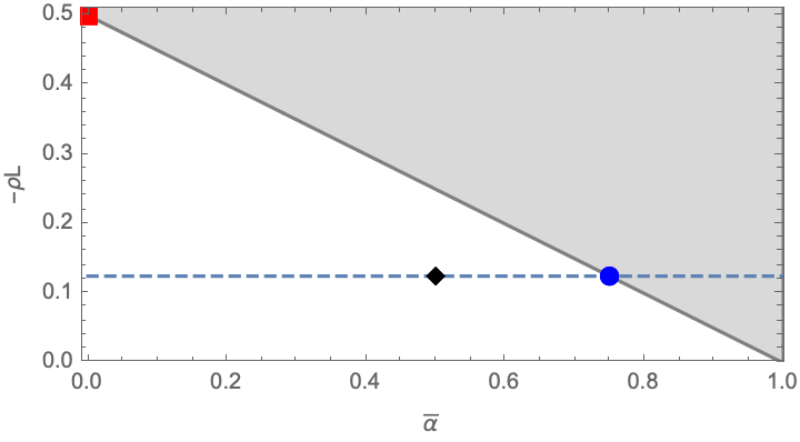
Figure 2: The grey region indicates where convergence provably cannot be guaranteed by Theorem 3.4. The dashed line indicates where $\rho=-\nicefrac{{1}}{{8L}}$. This is the condition under which (Diakonikolas et al., 2021, Thm. 3.2) shows the first convergence result $({\color[rgb]{0,0,0}\blackdiamond})$. Corollary 3.2 improves their result by matching the lower bound for any $\bar{\alpha}$, in particular for $\bar{\alpha}=\nicefrac{{3}}{{4}}$ $({\color[rgb]{0,0,1}\CIRCLE})$. The adaptive scheme in Theorem 3.1 matches the smallest possible $\rho$ for any (EG+) scheme with fixed stepsize $({\color[rgb]{1,0,0}\blacksquare})$.

4 Adaptively taking larger stepsizes using local curvature

Algorithm 2 Lipschitz constant backtracking

2.1:    $z^{k}\in\mathbb{R}^{n}$, $\tau\in(0,1)$, $\nu\in(0,1)$

2.2:     Set initial guess $\gamma=\gamma^{\rm init}$, and let $G_{\gamma}(z^{k})\coloneqq\big{(}{\rm id}+\gamma A\big{)}^{-1}\big{(}z^{k}-\gamma Fz^{k}\big{)}$ 2.3:    while $\gamma\|F(G_{\gamma}(z^{k}))-Fz^{k}\|>\nu\|G_{\gamma}(z^{k})-z^{k}\|$ do $\gamma\leftarrow\tau\gamma$

2.4:    $\gamma_{k}=\gamma$ and $\bar{z}^{k}=G_{\gamma}(z^{k})$

As made apparent in the analysis in Section 3 (cf. Section B.1) the bound on the smallest weak MVI constant $\rho$ in Item 3 may be replaced with the requirement that $\rho>-\nicefrac{{\gamma_{k}}}{{2}}$ for all $k\in\mathbb{N}$. Therefore, larger stepsizes $\gamma_{k}$ would guarantee global convergence for an even larger class of problems. Since a global Lipschitz constant is inherently pessimistic the natural question then becomes how to locally choose a maximal stepsize without diverging.

The proposed scheme involves a backtracking linesearch that uses the local curvature for its initial guess. The reason being that this will immediately pass, close enough to the solution $z^{\star}$, by argument of continuity. More precisely, we will set the initial guess to something slightly smaller than $\|JF(z^{k})\|^{-1}$, where $JF(z)$ denotes the Jacobian of $F$ at $z$ and $\|\cdot\|$ is the spectral norm. Note that, despite the use of second order information, the scheme remains efficient since $\|JF({}z{})[{}{}{}]\|$ only requires one eigenvalue computation performed through Jacobian-vector product (Pearlmutter, 1994).

Given an initial point $z^{0}=z^{\rm init}$ and $\nu\in(0,1)$, the final scheme which we denote (CurvatureEG+) proceeds for $k=0,1,\dots$ as follows:

$$\begin{split}1.\ &\text{Obtain $\gamma_{k}$ and $\bar{z}^{k}$ according to \lx@cref{creftypecap~refnum}{alg:LSBacktrack} with $\gamma^{\mathrm{init}}=\nu\|JF(z^{k})\|^{-1}$}\\ 2.\ &\text{Compute $z^{k+1}$ according to \lx@cref{creftypeplural~refnum}{State:alpha:Struct} and~\lx@cref{refnum}{state:Finito:s+:Struct} of \lx@cref{creftypecap~refnum}{alg:WeakMinty:Struct} }\end{split}$$ (CurvatureEG+)

The above intuitive reasoning is made precise in the next lemma where it is shown that backtracking linesearch will terminate in finite time and that $\gamma^{\mathrm{init}}$ will be immediately accepted asymptotically.

Lemma 4.1 (Lipschitz constant backtracking).

Suppose that $F:\mathbb{R}^{n}\to\mathbb{R}^{n}$ is a $L$-Lipschitz continuous operator. Consider the linesearch procedure in Algorithm 2. Then,

1. The linesearch terminates in finite time with $\gamma\geq\min\{\gamma^{\rm init},\nicefrac{{\nu\tau}}{{L}}\}$;

2. Suppose that $(z^{k})_{k\in\mathbb{N}}$ converges to $z^{\star}\in\operatorname*{zer}T$. If $F$ is continuously differentiable, and $\gamma^{\rm init}\in(0,\nu\|JF({}z^{k}{})[{}{}{}]\|^{-1})$ with $\nu\in(0,1)$, then eventually the backtrack will never be invoked ($\gamma^{\rm init}$ would be accepted).

The convergence results for (CurvatureEG+) are deduced based of the above lemma and Theorem 3.1 and are provided in Corollary B.1 in Section B.2. We illustrate the behavior of (CurvatureEG+) in Fig. 1 and in Section 6.

5 Constructing toy examples

When Item 3 holds for negative $\rho$, limit cycles of the underlying operator $Fz$ can emerge. We illustrate this with simple polynomial examples for which all the properties of interest can be computed in closed form.

Definition 1 (PolarGame).

A PolarGame denotes a two-player game whose associated operator $F$ has limit cycles at $\|z\|_{2}=c_{i}$ for all $i\in[k]$ where $c_{i}\neq 0$.

This turns out to be particularly easy to construct in polar coordinates as the name suggests (see Section C.1). Apart from introducing arbitrary number of limit cycles it also gives us control over $\rho$. This is illustrated in the following instantiations capturing three important cases.

Example 3: (PolarGame). Consider $Fz={\mathopen{}\left(\psi(x,y)-y,\psi(y,x)+x\right)\mathclose{}}$ where $\|z\|_{\infty}\leq\nicefrac{{11}}{{10}}$ and $\psi(x,y)=\frac{1}{16}ax(-1+x^{2}+y^{2})(-9+16x^{2}+16y^{2})$. We have the following three cases:

(i)  $a=1$ then $\rho\in(-\frac{1}{L},-\frac{1}{2L})$  (ii)  $a=\frac{3}{4}$ then $\rho\in(-\frac{1}{2L},-\frac{1}{3L})$  (iii)  $a=\frac{1}{3}$ then $\rho\in(-\frac{1}{8L},-\frac{1}{10L})$

where $L$ denotes the Lipschitz constant of $F$ restricted to the constraint set. For all cases $F$ exhibits limit cycles at $\|z\|=1$ and $\|z\|=\nicefrac{{3}}{{4}}$. Proof is deferred to Section C.2.

Example 4: (minimax). In the particular case of constrained minimax problem we introduce the following polynomial game:

$$\operatorname*{minimize}_{|x|\leq\nicefrac{{4}}{{3}}}\operatorname*{maximize}_{|y|\leq\nicefrac{{4}}{{3}}}\phi(x,y):=xy+\psi(x)-\psi(y),$$ (GlobalForsaken)

where $\psi(z)=\frac{2z^{6}}{21}-\frac{z^{4}}{3}+\frac{z^{2}}{3}$. We provide proof of the following properties in Section C.3:

1. There exists a repellant limit cycle and an attracting limit cycle of $F$.

2. $z^{\star}=(0,0)$ is a global Nash equilibrium for which Item 3 holds inside the constraint with $\rho>-\nicefrac{{1}}{{2L}}$, where $L$ denotes the Lipschitz constant of $F$ restricted to the constraint set.

6 Experiments

The algorithms considered in the experiments include the adaptive Algorithm 1, (CurvatureEG+), and constant stepsize methods that can be seen as instances of (CEG+) for various choices of $\gamma_{k}$ and $\bar{\alpha}_{k}$. When $\gamma_{k}=\nicefrac{{1}}{{L}}$ and $\bar{\alpha}_{k}=1$ we recover a constrained variant of extragradient, which we denote CEG. When $\bar{\alpha}_{k}=\nicefrac{{1}}{{2}}$ we denote the scheme CEG+, which is the direct generalization to the constraint setting of the (EG+) scheme studied in Diakonikolas et al. (2021, Thm. 3.2). Note that this choice of $\bar{\alpha}_{k}$ restricts the problem class for which we otherwise can have guaranteed convergence according to Corollary 3.2. When $\bar{\alpha}_{k}$ is chosen adaptively according to Algorithm 1 we refer to it as AdaptiveEG+. Finally, when $\gamma_{k}$ is additionally chosen adaptively we use the name (CurvatureEG+).

In the stochastic setting, when $\gamma_{k}=\nicefrac{{1}}{{k}}$ and $\alpha_{k}=1$, effectively both stepsizes diminish, and we recover a constrained variant of the popular stochastic extragradient scheme (see e.g. Hsieh et al. (2021, Algorithm 3)), which we refer to as SEG. We also consider a heuristic variant where $\gamma_{k}=\nicefrac{{1}}{{L}}$ and only $\alpha_{k}$ is decreasing, which we refer to as SEG+.

We test the algorithms on the constructed examples and confirm their convergence guarantees. Specifically, we apply the algorithms to the minimax problem in Definition 1, the PolarGames in Definition 1, and a worst case construction, Section B.3, from the proof of the lower bound (cf. Section B.3). For Section B.3 we choose the problem parameters such that $\rho=-\nicefrac{{1}}{{3L}}$ according to (B.13), and additionally add an $\ell_{\infty}$-ball constraint to keep the iterates bounded. To simulate the stochastic setting we add Gaussian noise to calls of $F$. Results for the deterministic setting and stochastic setting can be found in Fig. 3 and Fig. 4 respectively.

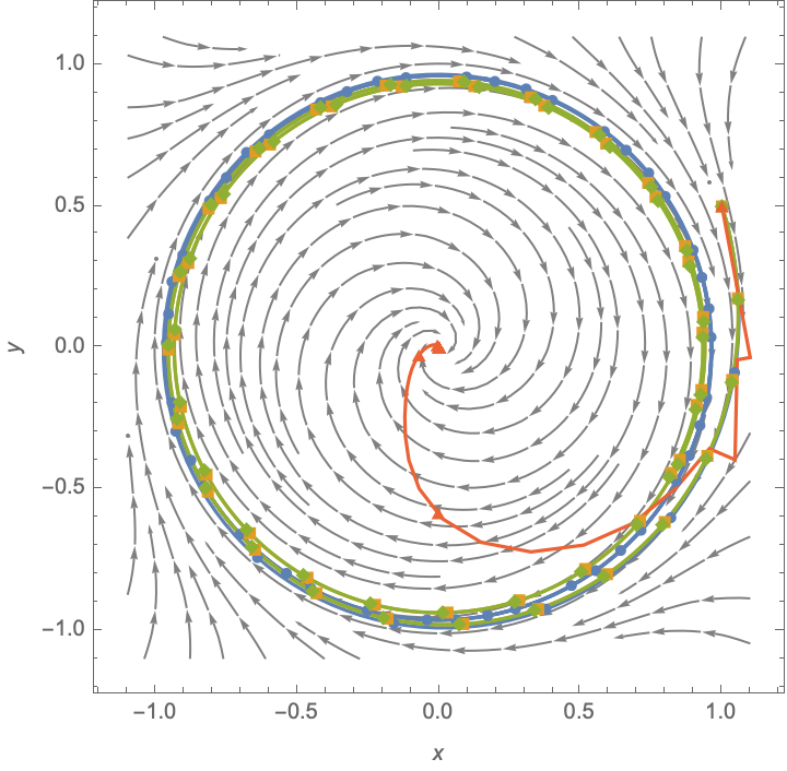
(a) Definition 1 ($a=1$)

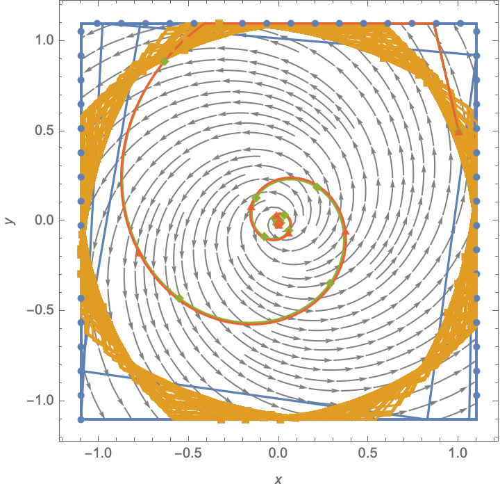
(b) Section B.3 ($\rho=-\nicefrac{{1}}{{3L}}$)

Figure 3: Deterministic setting. In (3(a)) we have an instance of Definition 1 with $\rho<-\nicefrac{{1}}{{2L}}$ for which Theorem 3.4 provides lower bound for extrapolation stepsize $\gamma_{k}=\nicefrac{{1}}{{L}}$. However, adaptively choosing $\gamma_{k}$ larger can converge as illustrated with (CurvatureEG+). In addition, (3(b)) confirms with Section B.3, that (CEG+) for $\bar{\alpha}_{k}=\nicefrac{{1}}{{2}}$ and CEG may indeed not converge even when $\rho=-\nicefrac{{1}}{{3L}}$. In contrast, both AdaptiveEG+ and (CurvatureEG+) converges to the stationary point. Note that picking $\bar{\alpha}_{k}<\nicefrac{{1}}{{3}}$ would lead to convergence of (CEG+) by Corollary 3.2. See Fig. 6 and Fig. 7 for supplementary experiments.

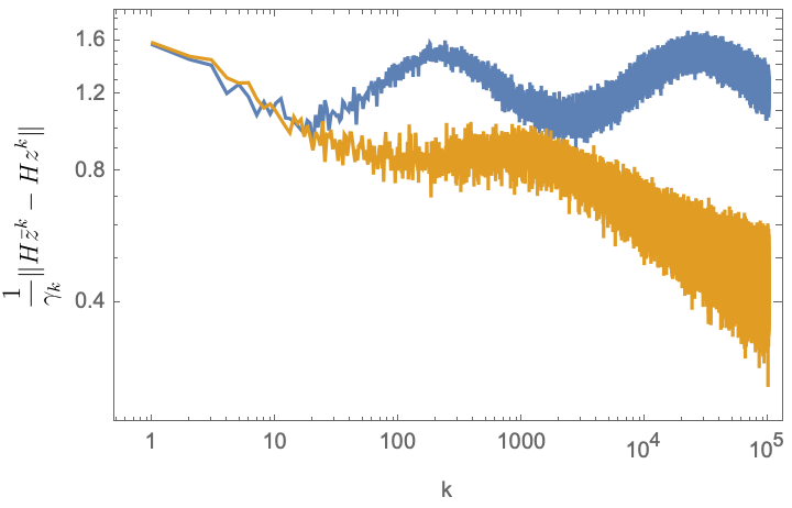
(a) Definition 1

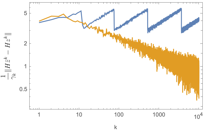
(b) Section B.3 ($\rho=-\nicefrac{{1}}{{3L}}$)

Figure 4: Stochastic setting. In (4(a)) we test the stochastic algorithms on our nonconvex-nonconcave constrained minimax example. The cycling behavior of SEG is inline with Hsieh et al. (2021), who shows that the sequence generated by SEG can converge to limit cycles of the underlying operator $F$. On the other hand, we observe that SEG+ escapes the attracting limit cycle. In (4(b)) we also provide a more challenging example motivated by our lower bound.

7 Conclusion

This paper introduced an EG-type algorithm for a class of nonconvex-nonconcave minimax problems that satisfy the weak Minty variational inequality (MVI). The range of parameter in the weak MVI was extended compared to EG+ of Diakonikolas et al. (2021), and tightness of our results were demonstrated through construction of a counter example. In addition, EG+ (Diakonikolas et al., 2021), as well as the forward-backward-forward algorithm (Tseng, 2000) were all shown to be special cases of our scheme. Furthermore, (CurvatureEG+) was proposed that performs a backtracking linesearch on the extrapolation stepsize $\gamma_{k}$ allowing for larger stepsizes and relaxes the condition $\rho>\tfrac{1}{2L}$ to $\rho>\nicefrac{{-\gamma_{k}}}{{2}}$ which is often a much weaker condition. More importantly, it is shown that asymptotically the linesearch always passes with $\gamma_{k}=\nu\|JF({}z^{k}{})[{}{}{}]\|^{-1}$ for any $\nu\in(0,1)$, thus ratifying the name (CurvatureEG+). Future direction include exploring applications of the proposed algorithm in particular in the setting of GANs. It is also interesting to develope a variance reduced variant of the algorithm for finite sum minimax problems.

8 Acknowledgments and disclosure of funding

We would like to especially thank Yu-Guan Hsieh for providing valuable feedback and discussion. This project has received funding from the European Research Council (ERC) under the European Union’s Horizon 2020 research and innovation programme (grant agreement n° 725594 - time-data). This work was supported by the Swiss National Science Foundation (SNSF) under grant number 200021_205011. The work of the second and third author was supported by the Research Foundation Flanders (FWO) postdoctoral grant 12Y7622N and research projects G081222N, G0A0920N, G086518N, and G086318N; Research Council KU Leuven C1 project No. C14/18/068; Fonds de la Recherche Scientifique – FNRS and the Fonds Wetenschappelijk Onderzoek – Vlaanderen under EOS project no 30468160 (SeLMA); European Union’s Horizon 2020 research and innovation programme under the Marie Skłodowska-Curie grant agreement No. 953348. The work of Olivier Fercoq was supported by the Agence National de la Recherche grant ANR-20-CE40-0027, Optimal Primal-Dual Algorithms (APDO).

Appendix A Preliminary definitions

Notationally we will use $\lfloor x\rfloor_{+}\coloneqq\max\{0,x\}$ throughout. We additionally recall some standard definitions and results and refer to Bauschke & Combettes (2017); Rockafellar (1970)) for further details.

An operator or set-valued mapping $A:\mathbb{R}^{n}\rightrightarrows\mathbb{R}^{d}$ maps each point $x\in\mathbb{R}^{n}$ to a subset $Ax$ of $\mathbb{R}^{d}$. We will use the notation $A(x)$ and $Ax$ interchangably. We denote the domain of $A$ by

$$\operatorname{dom}A\coloneqq\{x\in\mathbb{R}^{n}\mid Ax\neq\emptyset\},$$

its graph by

$$\operatorname{gph}A\coloneqq\{(x,y)\in\mathbb{R}^{n}\times\mathbb{R}^{d}\mid y\in Ax\},$$

and the set of its zeros by $\operatorname*{zer}A\coloneqq\{x\in\mathbb{R}^{n}\mid 0\in Ax\}$. The inverse of $A$ is defined through its graph: $\operatorname{gph}A^{-1}\coloneqq\{(y,x)\mid(x,y)\in\operatorname{gph}A\}$. The resolvent of $A$ is defined by $J_{A}\coloneqq({\rm id}+A)^{-1}$, where ${\rm id}$ denotes the identity operator.

Definition A.1 ((co)monotonicity Bauschke et al. (2020)).

An Operator $A:\mathbb{R}^{n}\rightrightarrows\mathbb{R}^{n}$ is said to be $\rho$-monotone for some $\rho\in\mathbb{R}$, if for all $(x,y),(x^{\prime},y^{\prime})\in\operatorname{gph}A$

$$\rho\|x-x^{\prime}\|^{2}\leq\langle x-x^{\prime},y-y^{\prime}\rangle,$$

and it is said to be $\rho$-comonotone if for all $(x,y),(x^{\prime},y^{\prime})\in\operatorname{gph}A$

$$\rho\|y-y^{\prime}\|^{2}\leq\langle x-x^{\prime},y-y^{\prime}\rangle.$$

The operator $A$ is said to be maximally (co)monotone if its graph is not strictly contained in the graph of another (co)monotone operator.

We say that $A$ is monotone if it is $0$-monotone. When $\rho<0$, $\rho$-comonotonicity is also referred to as $|\rho|$-cohypomonotonicity.

Definition A.2 (Lipschitz continuity and cocoercivity).

Let $\mathcal{D}\subseteq\mathbb{R}^{n}$ be a nonempty subset of $\mathbb{R}^{n}$. A single-valued operator $A:\mathcal{D}\to\mathbb{R}^{n}$ is said to be $L$-Lipschitz continuous if for any $x,x^{\prime}\in\mathcal{D}$

$$\|Ax-Ax^{\prime}\|\leq L\|x-x^{\prime}\|,$$

and $\beta$-cocoercive if

$$\beta\|Ax-Ax^{\prime}\|^{2}\leq\langle x-x^{\prime},Ax-Ax^{\prime}\rangle.$$

Moreover, $A$ is said to be nonexpansive if it is $1$-Lipschitz continuous, and firmly nonexpansive if it is $1$-cocoercive.

The resolvent operator $J_{A}$ is firmly nonexpansive (with $\operatorname{dom}J_{A}=\mathbb{R}^{n}$) if and only if $A$ is (maximally) monotone.

The following lemma plays an important role in our convergence analysis.

Lemma A.3.

Let $A:\mathbb{R}^{n}\to\mathbb{R}^{n}$ denote a single valued operator. Then,

1. $A$ is $1$-Lipschitz if and only if $T={\rm id}-A$ is $\nicefrac{{1}}{{2}}$-cocoercive.

2. If $A$ is $L$-Lipschitz, then $T={\rm id}-\eta A$, $\eta\in(0,\nicefrac{{1}}{{L}})$, is $(1-\eta L)$-monotone, and in particular $\|Tu-Tv\|\geq(1-\eta L)\|u-v\|$ for all $u,v\in\mathbb{R}^{n}$.

Proof.

The first claim follows directly from (Bauschke & Combettes, 2017, Prop.4.11). That $T$ is strongly monotone is a consequence of the Cauchy Schwarz inequality and Lipschitz continuity of $A$:

$$\langle Tv-Tu,v-u\rangle{}={} \|v-u\|^{2}-\eta\langle Av-Au,v-u\rangle{}\geq{}(1-\eta L)\|v-u\|^{2}.$$

In turn, the last claim follows from the Cauchy-Schwarz inequality. ∎

Appendix B Proofs and further results

B.1 Proofs of Section 3

 

Proof of Theorem 3.1.

Let $H={\rm id}-\gamma_{k}F$. By 1.3 $Hz^{k}\in\bar{z}^{k}+\gamma_{k}A\bar{z}^{k}$. Therefore,

$$\tfrac{1}{\gamma_{k}}(Hz^{k}-H\bar{z}^{k}){}\in{}A\bar{z}^{k}+F\bar{z}^{k}$$ (B.1)

In what follows we will show that Algorithm 1 is equivalent to taking a forward-backward step followed by a correction step. Consider the updates

$$\bar{z}^{k}{}\coloneqq{} {\mathopen{}\left({\rm id}+\gamma_{k}A\right)\mathclose{}}^{-1}\big{(}z^{k}-\gamma_{k}Fz^{k}\big{)},$$ (B.2)

$$z^{k+1}{}={} (1-\lambda_{k})z^{k}+\lambda_{k}\operatorname{\Pi}_{\mathcal{D}_{k}}(z^{k}),\quad\text{where}\quad\mathcal{D}_{k}\coloneqq{\mathopen{}\left\{w\mid\langle Hz^{k}-H\bar{z}^{k},\bar{z}^{k}-w\rangle\geq\tfrac{\delta_{k}}{\gamma_{k}}\|Hz^{k}-H\bar{z}^{k}\|^{2}{}\mid{}{}\right\}\mathclose{}}.$$

Note that

$$\langle H\bar{z}^{k}-Hz^{k},\bar{z}^{k}-z^{k}\rangle+\tfrac{\delta_{k}}{\gamma_{k}}\|H\bar{z}^{k}-Hz^{k}\|^{2}{}\geq{} (\tfrac{1}{2}+\tfrac{\delta_{k}}{\gamma_{k}})\|H\bar{z}^{k}-Hz^{k}\|^{2}$$ (B.3)

where in the inequality Item 1 was used. Hence, by (B.3) the stepsize $\alpha_{k}$ is positive and bounded away from zero. Moreover, if $z^{k}\in\mathcal{D}_{k}$, then from (B.3) we may conclude that $\|H\bar{z}^{k}-Hz^{k}\|\leq 0$ which implies that the generated sequence remains constant and $\bar{z}^{k}\in\operatorname*{zer}T$ (cf. (B.1)).

The projection onto $\mathcal{D}_{k}$ for any $v\notin\mathcal{D}_{k}$ is given by

$$\operatorname{\Pi}_{\mathcal{D}_{k}}(v)=v+\frac{\langle\bar{z}^{k}-v,Hz^{k}-H\bar{z}^{k}\rangle-\tfrac{\delta_{k}}{\gamma_{k}}\|Hz^{k}-H\bar{z}^{k}\|^{2}}{\|Hz^{k}-H\bar{z}^{k}\|^{2}}(Hz^{k}-H\bar{z}^{k})$$

Moreover, (B.1) together with Item 3 at $\bar{z}^{k}$ yields

$$\tfrac{1}{\gamma_{k}}\langle Hz^{k}-H\bar{z}^{k},\bar{z}^{k}-z^{\star}\rangle\geq\tfrac{\rho}{\gamma_{k}^{2}}\|Hz^{k}-H\bar{z}^{k}\|^{2}\geq\tfrac{\delta_{k}}{\gamma_{k}^{2}}\|Hz^{k}-H\bar{z}^{k}\|^{2},$$ (B.4)

thus ensuring $z^{\star}\in\mathcal{S}^{\star}\subseteq\mathcal{D}_{k}$. The projection onto $\mathcal{D}_{k}$ is then given by $\operatorname{\Pi}_{\mathcal{D}_{k}}(z^{k})=z^{k}+\alpha_{k}(H\bar{z}^{k}-Hz^{k}),$ where $\alpha_{k}$ is as in 1.4.

Finally, since the projection $\operatorname{\Pi}_{\mathcal{D}_{k}}$ is firmly nonexpansive, it follows from (Bauschke & Combettes, 2017, Cor. 4.41) that the mapping $(1-\lambda_{k}){\rm id}+\lambda_{k}\operatorname{\Pi}_{\mathcal{D}_{k}}$ is $\nicefrac{{\lambda_{k}}}{{2}}$-averaged. Consequently, we may conclude that $(z^{k})_{k\in\mathbb{N}}$ is Fejér monotone relative to $\mathcal{S}^{\star}$ (Bauschke & Combettes, 2017, Prop. 4.35(iii)). That is for all $z^{\star}\in\mathcal{S}^{\star}$

$$\|z^{k+1}-z^{\star}\|^{2}{}\leq{} \|z^{k}-z^{\star}\|^{2}-\lambda_{k}{(2-\lambda_{k})}\alpha_{k}^{2}\|H\bar{z}^{k}-Hz^{k}\|^{2}.$$

$$\text{\eqref{eq:posAlpha}}{}\leq{} \|z^{k}-z^{\star}\|^{2}-\tfrac{\varepsilon_{k}}{\gamma_{k}^{2}}\|H\bar{z}^{k}-Hz^{k}\|^{2},$$ (B.5)

where $\varepsilon_{k}\coloneqq\lambda_{k}(2-\lambda_{k})(\tfrac{\gamma_{k}}{2}+\delta_{k})^{2}$. The convergence rate in (3.1) is obtained by telescoping (B.5). Since $\liminf_{k\to\infty}\varepsilon_{k}>0$, $(\tfrac{1}{\gamma_{k}^{2}}\|H\bar{z}^{k}-Hz^{k}\|^{2})_{k\in\mathbb{N}}$ converges to zero. Moreover, $(\|z^{k}-z^{\star}\|^{2})_{k\in\mathbb{N}}$ converges and the sequence $(z^{k})_{k\in\mathbb{N}}$ is bounded. Since $\gamma_{k}$ is bounded, and $F$ and the resolvents $({\rm id}+\gamma_{k}A)^{-1}$ are Lipschitz continuous (cf. (Bauschke & Combettes, 2017, Cor. 23.9)), so is their composition. Hence, $(\bar{z}^{k})_{k\in\mathbb{N}}$ is also bounded. Let $(\bar{z}^{k})_{k\in K}$ be a subsequence converging to some $\bar{z}\in\mathbb{R}^{n}$. Combined with the fact that $(\tfrac{1}{\gamma_{k}^{2}}\|H\bar{z}^{k}-Hz^{k}\|^{2})_{k\in\mathbb{N}}$ converges to zero, we may conclude from (B.1) along with (Bauschke & Combettes, 2017, Prop. 20.38) and Lipschitz continuity of $F$ that $\bar{z}\in\operatorname*{zer}T$. Finally, if in addition $\gamma=\limsup_{k\to\infty}\gamma_{k}<1/L$, then $(1-\gamma L)\|\bar{z}^{k}-z^{k}\|\leq\|H\bar{z}^{k}-Hz^{k}\|$ (invoke Item 2). Therefore, $(\|\bar{z}^{k}-z^{k}\|)_{k\in\mathbb{N}}$ converges to zero, which in turn implies that a subsequence $(z^{k})_{k\in K^{\prime}}$ converges to a point $z^{\prime}$ iff so does the subsequence $(\bar{z}^{k})_{k\in K^{\prime}}$. Hence, $(z^{k})_{k\in K}$ also converges to $\bar{z}\in\operatorname*{zer}T$. Consequently, if Item 3 holds at all of the zeros of $T$, i.e., if $\mathcal{S}^{\star}=\operatorname*{zer}T$, then the second claim follows by invoking (Bauschke & Combettes, 2017, Thm. 5.5). ∎

 

 

Proof of Corollary 3.2.

The proof of convergence was already given prior to the statement of the corollary. It remains to derive (3.3). By Item 3 and owing to $\nicefrac{{1}}{{2}}$-cocoercivity of $H$ (cf. Item 1)

$$\langle z^{k}-z^{\star},H{\bar{z}^{k}}-H{z^{k}}\rangle{}={} \langle\bar{z}^{k}-z^{\star},H{\bar{z}^{k}}-H{z^{k}}\rangle{}+{}\langle z^{k}-{\bar{z}^{k}},H{\bar{z}^{k}}-H{z^{k}}\rangle$$

$$\text{\eqref{eq:mintyH}}{}\leq{} -(\tfrac{1}{2}+\tfrac{\delta_{k}}{\gamma_{k}})\|H\bar{z}^{k}-Hz^{k}\|^{2}.$$ (B.6)

Therefore, provided that $\bar{\alpha}>0$ we have

$$\|z^{k+1}-z^{\star}\|^{2}{}={} \|z^{k}-z^{\star}\|^{2}+\bar{\alpha}^{2}\|H\bar{z}^{k}-Hz^{k}\|^{2}+2\bar{\alpha}\langle z^{k}-z^{\star},H\bar{z}^{k}-Hz^{k}\rangle$$

$$\text{\eqref{eq:innprodlower}}{}\leq{} \|z^{k}-z^{\star}\|^{2}-\bar{\alpha}(2(\tfrac{1}{2}+\tfrac{\delta}{\gamma})-\bar{\alpha})\|H\bar{z}^{k}-Hz^{k}\|^{2}.$$

Telescoping the above inequality yields the claimed inequality. ∎

 

B.2 Convergence results and proofs of Section 4

The convergence results for (CurvatureEG+) are provided in the next corollary where $\rho$ in Item 3 is allowed to take potentially larger values provided that $\rho>-\nicefrac{{\gamma_{k}}}{{2}}$. Note that owing to the lower bound on $\gamma_{k}$ (cf. Item 1), the weak MVI assumption in the corollary is always satisfied if $\rho\in(-\nicefrac{{\nu\tau}}{{2L}},\infty)$, however, in practice $\gamma_{k}$ may take larger values.

Corollary B.1.

Suppose that Items 1 and 2 hold, and consider the sequences $(z^{k})_{k\in\mathbb{N}}$, $(\bar{z}^{k})_{k\in\mathbb{N}}$ generated by (CurvatureEG+). Suppose that Item 3 holds for some $\rho\in\mathbb{R}$ satisfying $\gamma_{k}+2\rho>0$, and let ${\delta_{k}\in(\nicefrac{{-\gamma_{k}}}{{2}},\rho]}$, $\lambda_{k}\in(0,2)$, $\liminf_{k\to\infty}\lambda_{k}(2-\lambda_{k})>0$, and $\liminf_{k\to\infty}(\delta_{k}+\nicefrac{{\gamma_{k}}}{{2}})>0$. Then,

1. The sequence $(\|\bar{z}^{k}-z^{k}\|^{2})_{k\in\mathbb{N}}$ vanishes;

2. $(\bar{z}^{k})_{k\in\mathbb{N}}$, $(z^{k})_{k\in\mathbb{N}}$ are bounded, and have the same limit points belonging to $\operatorname*{zer}T$;

3. if in addition $\mathcal{S}^{\star}=\operatorname*{zer}T$, then $(z^{k})_{k\in\mathbb{N}}$, $(\bar{z}^{k})_{k\in\mathbb{N}}$ both converge to some $z^{\star}\in\operatorname*{zer}T$.

Moreover, if $z^{k},\bar{z}^{k}\to z^{\star}\in\operatorname*{zer}T$ (as is the case in 3), and $F$ is continuously differentiable, then eventually the backtrack will never be invoked.

Proof.

Observe that in the proof of Theorem 3.1 $1$-Lipschitz continuity of $\gamma_{k}F$ is only used at the generated points $\bar{z}^{k}$ and $z^{k}$ (see (B.3)), and is thus ensured by the linesearch Algorithm 2. Therefore, it is easy to see that $\alpha_{k}$ is positive and bounded away from zero provided that $\rho>-\nicefrac{{\gamma_{k}}}{{2}}$ , see (B.3). Moreover, since $\gamma_{k}\|F\bar{z}^{k}-Fz^{k}\|\leq\nu\|\bar{z}^{k}-z^{k}\|$, arguing as in Item 2 we obtain $\|H\bar{z}^{k}-Hz^{k}\|\geq(1-\nu)\|\bar{z}^{k}-z^{k}\|$. Hence, it follows from (B.5) that

$$\|z^{k+1}-z^{\star}\|^{2}{}\leq{} \|z^{k}-z^{\star}\|^{2}-\tfrac{\varepsilon_{k}(1-\nu)}{\gamma_{k}^{2}}\|\bar{z}^{k}-z^{k}\|^{2},$$

By telescoping the inequality and noting that $\gamma_{k}$ is bounded, we obtain $\sum_{k\in\mathbb{N}}\|\bar{z}^{k}-z^{k}\|^{2}<\infty$, implying 1. Noting this and arguing as in the last part of the proof of Theorem 3.1 establishes 2, 3. The last claim is the direct consequence of Item 2. ∎

 

Proof of Lemma 4.1.

1: Since $F$ is $L$-Lipschitz continuous the linesearch would terminate in finite steps. Either $\gamma^{\rm init}$ satisfies the condition, or else the backtrack procedure is invoked, which in turn implies the previous candidate $\gamma/\tau$ should have violated the condition leading the the claimed lower bound.

2: Since the resolvent $({\rm id}+\gamma A)^{-1}$ and $F$ are Lipschitz continous, so is their composition. Hence, $G_{\gamma}(z^{k})\to G_{\gamma}(z^{\star})$. Furthermore, by definition $z^{\star}-\gamma Fz^{\star}\in G_{\gamma}(z^{\star})+\gamma A(G_{\gamma}(z^{\star}))$. Consequently, using monotonicity of $A$ at $G_{\gamma}(z^{\star})$ and $z^{\star}$, and that $-Fz^{\star}\in Az^{\star}$ yields $0{}\leq{}\langle z^{\star}-\gamma Fz^{\star}-G_{\gamma}(z^{\star})+Fz^{\star},G_{\gamma}(z^{\star})-z^{\star}\rangle{}={}-\|z^{\star}-G_{\gamma}(z^{\star})\|^{2}$. Thus $G_{\gamma}(z^{\star})=z^{\star}$. Using the fact that both $(G_{\gamma}(z^{k}))_{k\in\mathbb{N}}$ and $(z^{k})_{k\in\mathbb{N}}$ converges to $z^{\star}\in\operatorname*{zer}T$:

$$\lim_{k\to\infty}\frac{\|F(G_{\gamma}(z^{k}))-Fz^{k}\|}{\|G_{\gamma}(z^{k})-z^{k}\|}{}\leq{}\limsup_{z,z^{\prime}\to z^{\star}}\frac{\|Fz^{\prime}-Fz\|}{\|z^{\prime}-z\|}{}={}\operatorname{lip}F(z^{\star}){}={}\|JF({}z^{\star}{})[{}{}{}]\|,$$

where (Rockafellar & Wets, 2009, Thm. 9.7) was used. The claim follows from continuity of $JF$ and the fact that $(z^{k})_{k\in\mathbb{N}}$ converges to $z^{\star}$. ∎

 

B.3 Proofs of Section 3.2

To prove the lower bound we introduce the following unconstrained bilinear minimax problem with an unstable critical point.

Example 5: Consider the following minimax problem:

$$\operatorname*{minimize}_{x\in\mathbb{R}}\operatorname*{maximize}_{y\in\mathbb{R}}f(x,y):=axy+\frac{b}{2}(x^{2}-y^{2}),$$ (B.7)

where $b<0$ and $a>0$.

 

Proof of Theorem 3.4.

The associated operator of Section B.3 can easily be computed,

$$Fz={\mathopen{}\left(ay+bx,by-ax\right)\mathclose{}},$$ (B.8)

where $z=(x,y)$. In this particular case, both $L$ and $\rho$ turn out to be constants. By simple calculation we have,

$$\|JF(z)\|=\sqrt{a^{2}+b^{2}},\quad\rho=\frac{b}{a^{2}+b^{2}}$$ (B.9)

where $\|\cdot\|$ is the spectral norm. Since the norm of the Jacobian is constant it equates the global Lipschitz constant, $L=\|JF(z)\|$.

By linearity of $F$, one step of (EG+) is conveniently also a linear operator. Specifically,

$$z^{k+1}=Tz^{k}\quad\text{with}\quad T:={\mathopen{}\left(\begin{array}[]{cc}\frac{(1-\bar{\alpha})a^{2}+b{\mathopen{}\left(-\bar{\alpha}\sqrt{a^{2}+b^{2}}+\bar{\alpha}b+b\right)\mathclose{}}}{a^{2}+b^{2}}&-\frac{a\bar{\alpha}{\mathopen{}\left(\sqrt{a^{2}+b^{2}}-2b\right)\mathclose{}}}{a^{2}+b^{2}}\\ \frac{a\bar{\alpha}{\mathopen{}\left(\sqrt{a^{2}+b^{2}}-2b\right)\mathclose{}}}{a^{2}+b^{2}}&\frac{(1-\bar{\alpha})a^{2}+b{\mathopen{}\left(-\bar{\alpha}\sqrt{a^{2}+b^{2}}+\bar{\alpha}b+b\right)\mathclose{}}}{a^{2}+b^{2}}\\ \end{array}\right)\mathclose{}}.$$ (B.10)

We know that a linear dynamical system is globally asymptotically stable if and only if the spectral radius of the linear mapping is strictly less than 1.

Let $\lambda_{1},\lambda_{2}$ be the eigenvalues of $T$. Then the spectral radius is the largest absolute value of the eigenvalues. For $T$ this becomes,

$$\max_{i\in\{1,2\}}|\lambda_{i}|=\sqrt{\frac{(2(\bar{\alpha}-1)\bar{\alpha}+1)a^{2}-2\bar{\alpha}(\bar{\alpha}+1)b{\mathopen{}\left(\sqrt{a^{2}+b^{2}}-b\right)\mathclose{}}+b^{2}}{a^{2}+b^{2}}}.$$ (B.11)

So we can ask what $c$ in $\rho=-\frac{c}{L}$ needs to be for the sequence $(z^{k})_{k\in\mathbb{N}}$ to converge. Solving for $c$ in this equality with $\max_{i}|\lambda_{i}|<1$, we obtain,

$$c<\frac{1-\bar{\alpha}}{2},$$ (B.12)

provided that we pick

$$\frac{\sqrt{1-c^{2}}}{c}=-\frac{a}{b}.$$ (B.13)

Equation (B.13) provides a specification for Section B.3. As long as (B.12) is satisfied, (EG+) is guaranteed to converge for $\gamma_{k}=\nicefrac{{1}}{{L}}$. On the other hand, since (B.10) is a linear system, we simultaneously learn that picking $c$ any larger would imply non-convergence through $\max_{i}|\lambda_{i}|\geq 1$ (given $z^{0}\neq 0$). We can trivially embed problem (B.10) into a higher dimension to generalize the result. Noting that $c=-\rho L$ completes the proof. ∎

  We provide Mathematica code to verify each step of the above proof.

Appendix C Toy examples

In the following appendix, $L$ denotes the Lipschitz constant of $F$ restricted to the constraint set and $\rho$ is the parameter of the weak MVI (Item 3) when restricted to the constraint set. This restriction of the definitions is warranted, since $z^{k}$ remains within the constraint set in all simulations, while $\bar{z}^{k}$ is guaranteed to stay within by definition of 1.3 in Algorithm 1 (and likewise for all other considered method treating problem (2.1)).

All computer-assisted calculations can be found in the supplementary code.¹

C.1 Constructing a PolarGame (Definition 1)

Recall Definition 1 which considers a vectorfield $F:\mathbb{R}^{n}\rightarrow\mathbb{R}^{n}$ with limit cycles at $r\in{\mathopen{}\left\{c_{1},...,c_{k}{}\mid{}{}\right\}\mathclose{}}$ where $c_{i}\neq 0$ for all $i\in[k]$. Such a vectorfield can be constructed for $n=2$ by departing from the following dynamics in polar coordinates,

$$\begin{split}\frac{\partial r}{\partial t}&=-a\cdot r(t)\prod_{i=1}^{k}(r(t)+c_{i})\cdot(r(t)-c_{i})\\ \frac{\partial\theta}{\partial t}&=-b\cdot r(t),\end{split}$$ (C.1)

with $a,b\neq 0$. Transforming this dynamics into cartesian coordinates yields the desired vectorfield, $F$, while subsequently integrating with respect to $x$ and $y$ yields the two potentials associated with the two players. Note that the roots ${\mathopen{}\left\{-c_{i}{}\mid{}{}\right\}\mathclose{}}_{i=1}^{k}$ for the polynomial defining $\dot{r}$ are not strictly necessary for showing existence of limit cycles, but leads to a simpler form for $Fz$. We illustrate the construction in Fig. 5.

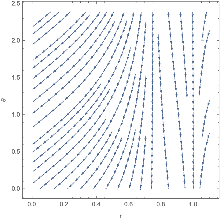
    $\Longrightarrow$

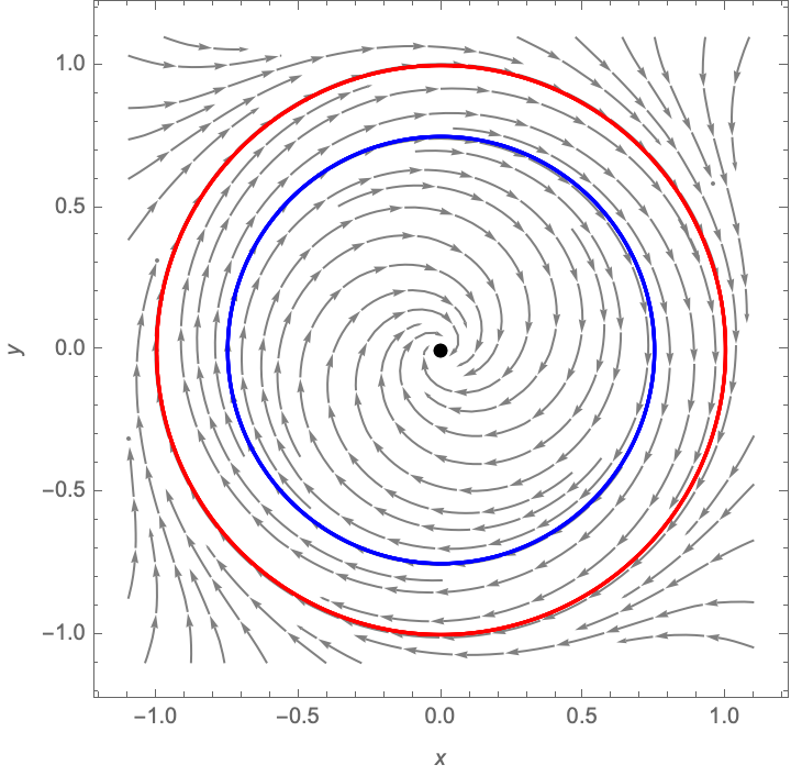
Figure 5: We can construct the desired properties in polar coordinates $(r,\theta)$ and subsequently transform it into a vectorfield in cartesian coordinates $(x,y)$. This is illustrated by a PolarGame with attracting limit cycles at radius $\|z\|=1$ and repellant limit cycle at $\|z\|=\nicefrac{{3}}{{4}}$ for the associated operator $Fz$ as indicated in red and blue respectively.

Proposition 1.

Let $Fz=(\dot{x},\dot{y})$ be the evolution in cartesian coordinates of the associated vectorfield in polar coordinates defined by (C.1). Then the only stationary point of $F$ is at the origin $(0,0)$ and there exists a limit cycle at $r=c_{i}$ for all $i\in[k]$.

Proof.

Let $r=\sqrt{x^{2}+y^{2}}$. It is easy to see from (C.1) that the only stationary point is at $r=0$. By construction, $\dot{r}$ is a polynomial with roots $c_{i}$ for all $i\in[k]$, so any trajectory starting on the circle defined by $r=c_{i}$ remains in that set. However, $\dot{\theta}$ is strictly nonzero. As a consequence $Fz$ is nonzero, so $r=c_{i}$ must define a limit cycle, which proofs the claim. ∎

(a) $a=1$

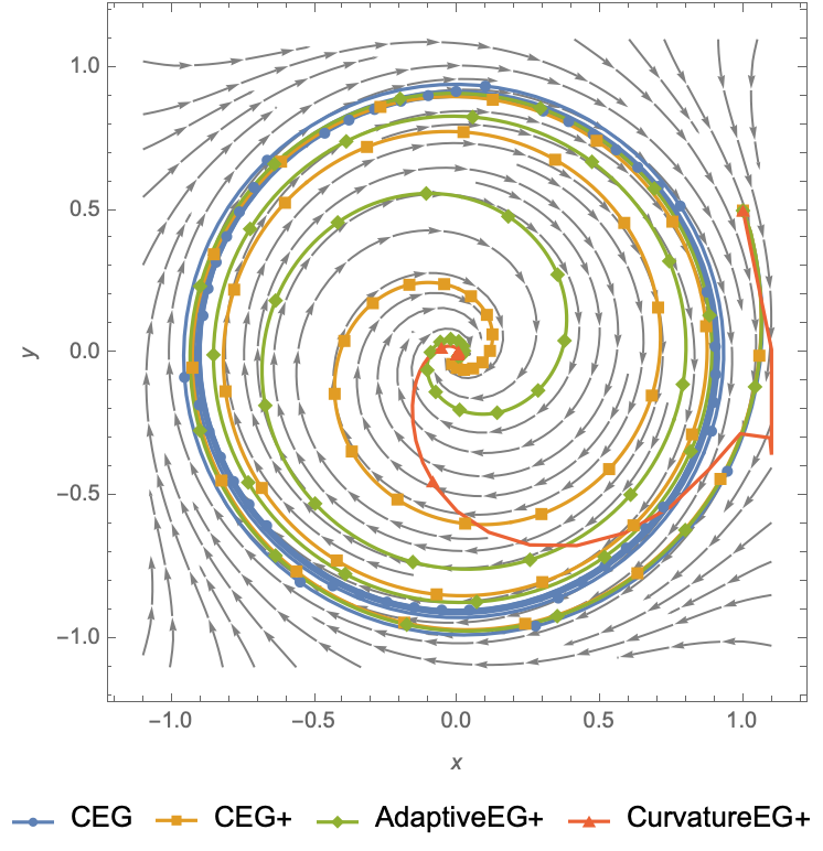
(b) $a=\nicefrac{{3}}{{4}}$

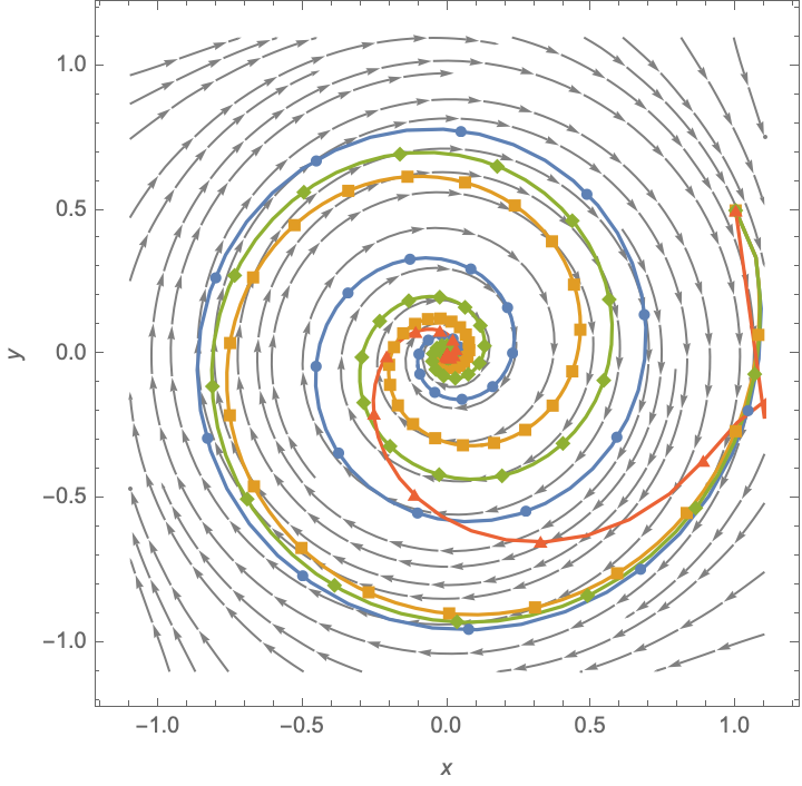
(c) $a=\nicefrac{{1}}{{3}}$

Figure 6: Definition 1 for different values of $a$ (and thereby different values of $\rho$). Note that even extragradient may escape the limit cycles even though $\rho<0$. This is not in conflict with the negative results of Hsieh et al. (2021) since the stepsize is not diminishing. However, in the general case even extragradient with fixed stepsize will not converge as shown by the lower bound in Theorem 3.4.

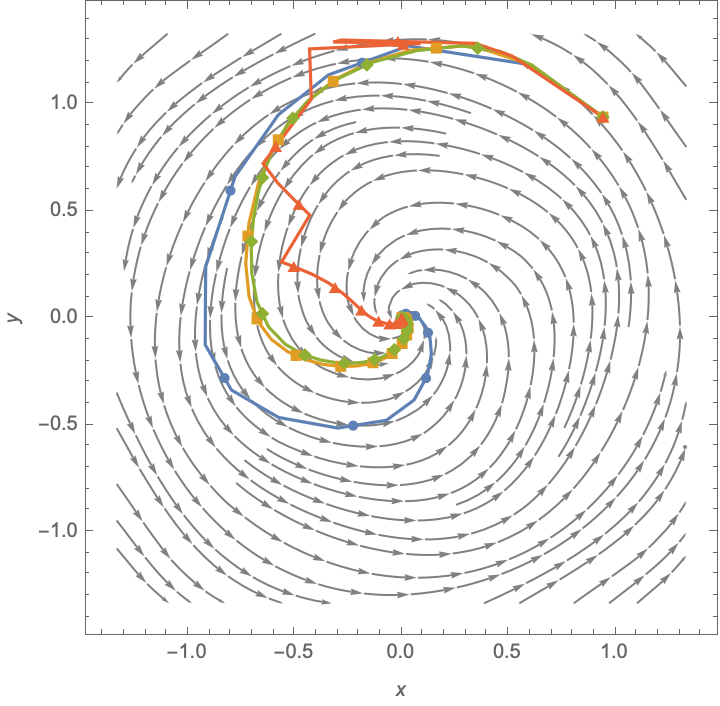
(a) Definition 1

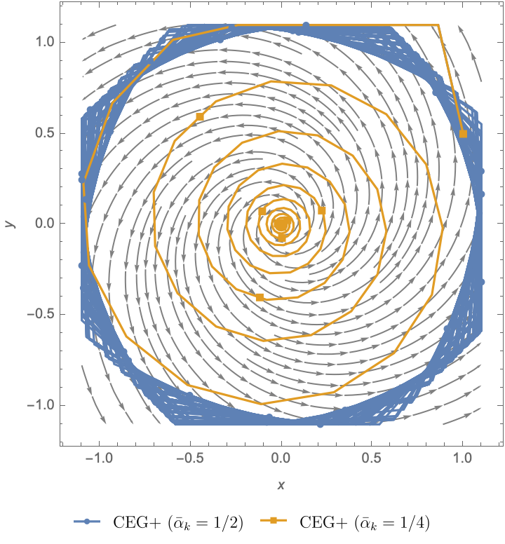
(b) Section B.3 ($\rho=\nicefrac{{1}}{{3L}}$)

Figure 7: In (7(a)) we observe that all algorithms converge, despite $F$ having an attracting limit cycle in Definition 1. However, note that in the stochastic setting, where diminishing stepsize is required, SEG does not converge to the critical point (see Fig. 4(a)). In (7(b)) we demonstrate that when $\rho=-\nicefrac{{1}}{{3L}}$, picking $\bar{\alpha}_{k}<\nicefrac{{1}}{{3}}$ for (CEG+) is necessary for convergence in general. See Section 6 for the experimental setup.

C.2 Proof for properties of Definition 1

The operator $F:\mathbb{R}^{2}\rightarrow\mathbb{R}^{2}$ defined in Definition 1 is obtained by constructing the associated dynamics in polar coordinates,

$$\begin{split}\frac{\partial r}{\partial t}&=-a\cdot r(t)\cdot(r(t)+1)\cdot(r(t)-1)\cdot(r(t)+\nicefrac{{3}}{{4}})\cdot(r(t)-\nicefrac{{3}}{{4}})\\ \frac{\partial\theta}{\partial t}&=-r(t).\end{split}$$ (C.2)

This can easily be verified by a change of variables. From Proposition 1 it then follows, that there must exist a limit cycle at $\|z\|=1$ and $\|z\|=\nicefrac{{3}}{{4}}$. To verify the conditions on $\rho$ we compute the closed form solution to $\rho$ and $L$ in Mathematica:

1. For $a=1$ we have $\rho=-\frac{50176}{1050977}$ and $L=\frac{\sqrt{2538096\sqrt{704424929}+70246989617}}{20000}$

2. For $a=\nicefrac{{3}}{{4}}$ we have $\rho=-\frac{602112}{16798825}$ and $L=\frac{\sqrt{7614288\sqrt{6383574361}+635022906553}}{80000}$

3. For $a=\nicefrac{{1}}{{3}}$ we have $\rho=-\frac{150528}{9439585}$ and $L=\frac{\sqrt{2538096\sqrt{754424929}+73446989617}}{60000}$

It can easily be verified that the stated conditions for $\rho$ in Definition 1 are met for the values above. This completes the proof.

We provide Mathematica code verifying the construction of $F$ and the closed form solutions to $L$ and $\rho$.

C.3 Proof for properties of Definition 1

Under the definitions of $\rho$ and $L$ in Appendix C, we claim that the origin $(0,0)$ in (GlobalForsaken) is a global Nash equilibrium and satisfies Item 3 with $\rho>-\nicefrac{{1}}{{2L}}$.

To verify that $(0,0)$ is indeed a global Nash equilibrium we need to check that the solution cannot be unilaterally improved. In other words, the solution should coincide with $(x^{\star},y^{\star})$ where

$$\begin{split}x^{\star}&=\operatorname*{arg\,min}_{x}\phi(x,0)\\ y^{\star}&=\operatorname*{arg\,max}_{y}\phi(0,y).\end{split}$$ (C.3)

We can easily verify this with Minimize in Mathematica, since the functions are polynomial for which a closed form solutions to the global optimization problem will be returned.

To find $\rho$ for $z^{\star}=(0,0)$ we solve the global minimization problem,

$$\operatorname*{minimize}_{z}\frac{\langle Fz,z-z^{\star}\rangle}{\|Fz\|^{2}},$$ (C.4)

for which a closed form solution can be found with Mathematica, which when numerically evaluated is approximately $-0.119732$.

We need to compute $L$ to ensure $\rho>-\nicefrac{{1}}{{2L}}$. In our case of convex constraints, $\mathcal{C}$, we have that $L=\sup_{z\in\mathcal{C}}\|JF(z)\|$ where $\|\cdot\|$ denotes the spectral norm (Rockafellar & Wets, 2009, Thm. 9.2 and 9.7). Under our constraint $\|z\|_{\infty}\leq\nicefrac{{4}}{{3}}$, this can similarly be computed in closed form, yielding $L=\nicefrac{{\sqrt{\frac{1}{2}{\mathopen{}\left(9409\sqrt{59721901}+74125591\right)\mathclose{}}}}}{{2835}}$. So $-\frac{1}{2L}\approx-0.165432$ which satisfy the condition $\rho>-\frac{1}{2L}$. This completes the proof.

Proposition 2.

Let $F$ be the associated operator of $\phi$ in (GlobalForsaken) defined as $Fz=({\nabla}_{x}\phi(x,y),-{\nabla}_{y}\phi(x,y))$. Define the radius as $r=\|z\|$. Then, $Fz$ has a stable critical point at the origin $(0,0)$, at least one attracting limit cycle in the region defined by $\sqrt{\nicefrac{{3}}{{2}}}<r<2$ and at least one repellant limit cycle within $r\leq\sqrt{\nicefrac{{3}}{{2}}}$.

Proof.

We follow a similar argument as in Hsieh et al. (2021, D.2). We can compute the associated operator $F$,

$${\mathopen{}\left(\begin{array}[]{c}\dot{x}\\ \dot{y}\end{array}\right)\mathclose{}}={\mathopen{}\left(\begin{array}[]{c}\frac{4x^{5}}{7}-\frac{4x^{3}}{3}+\frac{2x}{3}+y\\ -x+\frac{4y^{5}}{7}-\frac{4y^{3}}{3}+\frac{2y}{3}\\ \end{array}\right)\mathclose{}}.$$ (C.5)

With a change of variables into polar coordinates $(r,\theta)$ we get that $r=\sqrt{x^{2}+y^{2}}$ evolves as,

$$\dot{r}=-\frac{1}{42}r{\mathopen{}\left(9r^{4}\cos(4\theta)-14r^{2}\cos(4\theta)+15r^{4}-42r^{2}+28\right)\mathclose{}}.$$ (C.6)

When $r=\sqrt{\nicefrac{{3}}{{2}}}$ this reduces to $\dot{r}=\frac{3\cos(4\theta)+5}{56\sqrt{6}}$ and we observe that $\dot{r}>0$ for any $\theta$. Likewise for $r=2$, we have that $\dot{r}=-\frac{4}{21}(22\cos(4\theta)+25)$ which implies $\dot{r}<0$. Since there is no stationary point in the region $\mathcal{S}={\mathopen{}\left\{(r,\theta):\sqrt{\nicefrac{{3}}{{2}}}<r<2{}\mid{}{}\right\}\mathclose{}}$ it then follows from the Poincaré-Bendixson theorem (Teschl, 2012, Thm. 7.16) that there must exist at least one attracting limit cycle in $\mathcal{S}$. Further, it is easy to see that $(0,0)$ is a critical point and that it is stable by inspection of the Jacobian $JF(z)$. Since $\mathcal{S}$ is trapping, it follows from Poincaré–Hopf index theorem, that there must exist a repellant limit cycles in the region defined by $r<\sqrt{\nicefrac{{3}}{{2}}}$. This completes the proof. ∎

C.4 Proof of properties for (Hsieh et al., 2021, Example 5.2)

This section considers (Hsieh et al., 2021, Example 5.2) on the constraint domain $\mathcal{D}=\{z\in\mathbb{R}^{n}\mid\|z\|_{\infty}\leq\nicefrac{{3}}{{2}}\}$. We show that the unique critical point $z^{\star}$ does not satisfies the weak MVI for $\rho>-\nicefrac{{1}}{{2L}}$ even when restricted to the constraint set $z\in\mathcal{D}$. We restate the example with the additional constraint for convenience.

Example 6: (Hsieh et al., 2021, Example 5.2)

$$\operatorname*{minimize}_{|x|\leq\nicefrac{{3}}{{2}}}\operatorname*{maximize}_{|y|\leq\nicefrac{{3}}{{2}}}\phi(x,y):=x(y-0.45)+\psi(x)-\psi(y),$$ (Forsaken)

where $\psi(z)=\frac{1}{4}z^{2}-\frac{1}{2}z^{4}+\frac{1}{6}z^{6}$.

By using Mathematica, we can obtain a closed form solution of the Lipschitz constant $L$ of $F$ restricted to the constraint set, which we find to be $L=\frac{1}{80}\sqrt{\frac{1}{2}{\mathopen{}\left(1089\sqrt{801761}+993841\right)\mathclose{}}}$. Mathematica can solve approximately for the critical point, yielding $z^{\star}=(0.0780267,0.411934)$. To find $\rho$ we want to globally minimize $\rho(z):=\frac{{\mathopen{}\left\langle Fz,z-z^{\star}\right\rangle\mathclose{}}}{\|Fz\|^{2}}$ for $z\in\mathcal{D}$. Mathematica finds the candidate $z^{\prime}=(-1.01236,-0.104749)$ for which $\rho(z^{\prime})=-0.477761$. So $\rho$ must be at least this small, i.e. $\rho<-0.477761$. Since $-\nicefrac{{1}}{{2L}}\approx-0.04$, this implies that $\rho<-\nicefrac{{1}}{{2L}}$. See Forsaken.nb for Mathematica-assisted computations.

This rules out convergence guarantees for both (CEG+) and AdaptiveEG+ (Algorithm 1), which is supported by the simulation in Figure 8. However, as observed, (CurvatureEG+) converges in the simulations.

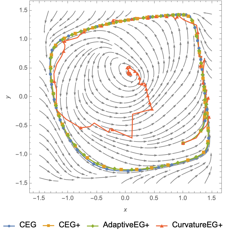
Figure 8: Demonstration of algorithms on (Hsieh et al., 2021, Example 5.2). Only (CurvatureEG+) converges to the critical point, while the remaining methods, CEG, (CEG+) with $\bar{\alpha}_{k}=\nicefrac{{1}}{{2}}$, and AdaptiveEG+ converges to an attracting limit cycle. See Section 6 for further specification of the algorithms.

References

- Azizian et al. (2020) Waïss Azizian, Ioannis Mitliagkas, Simon Lacoste-Julien, and Gauthier Gidel. A tight and unified analysis of gradient-based methods for a whole spectrum of differentiable games. In International Conference on Artificial Intelligence and Statistics, pp. 2863–2873. PMLR, 2020.
- Bauschke & Combettes (2017) Heinz H. Bauschke and Patrick L. Combettes. Convex analysis and monotone operator theory in Hilbert spaces. CMS Books in Mathematics. Springer, 2017. ISBN 978-3-319-48310-8.
- Bauschke et al. (2020) Heinz H Bauschke, Walaa M Moursi, and Xianfu Wang. Generalized monotone operators and their averaged resolvents. Mathematical Programming, pp. 1–20, 2020.
- Benaım & Hirsch (1999) Michel Benaım and Morris W Hirsch. Mixed equilibria and dynamical systems arising from fictitious play in perturbed games. Games and Economic Behavior, 29(1-2):36–72, 1999.
- Bertsekas (1997) Dimitri P Bertsekas. Nonlinear programming. Journal of the Operational Research Society, 48(3):334–334, 1997.
- Böhm et al. (2020) Axel Böhm, Michael Sedlmayer, Ernö Robert Csetnek, and Radu Ioan Boţ. Two steps at a time–taking gan training in stride with tseng’s method. arXiv preprint arXiv:2006.09033, 2020.
- Daskalakis et al. (2021a) Constantinos Daskalakis, Dylan J Foster, and Noah Golowich. Independent policy gradient methods for competitive reinforcement learning. arXiv preprint arXiv:2101.04233, 2021a.
- Daskalakis et al. (2021b) Constantinos Daskalakis, Stratis Skoulakis, and Manolis Zampetakis. The complexity of constrained min-max optimization. In Proceedings of the 53rd Annual ACM SIGACT Symposium on Theory of Computing, pp. 1466–1478, 2021b.
- Davis & Drusvyatskiy (2018) Damek Davis and Dmitriy Drusvyatskiy. Stochastic subgradient method converges at the rate $O(k{̂-1/4})$ on weakly convex functions. arXiv:1802.02988 [cs, math], February 2018.
- Diakonikolas et al. (2021) Jelena Diakonikolas, Constantinos Daskalakis, and Michael Jordan. Efficient methods for structured nonconvex-nonconcave min-max optimization. In International Conference on Artificial Intelligence and Statistics, pp. 2746–2754. PMLR, 2021.
- Facchinei & Pang (2007) Francisco Facchinei and Jong-Shi Pang. Finite-dimensional variational inequalities and complementarity problems. Springer Science & Business Media, 2007.
- Fiez & Ratliff (2020) Tanner Fiez and Lillian Ratliff. Gradient descent-ascent provably converges to strict local minmax equilibria with a finite timescale separation. arXiv preprint arXiv:2009.14820, 2020.
- Gidel et al. (2018) Gauthier Gidel, Hugo Berard, Gaëtan Vignoud, Pascal Vincent, and Simon Lacoste-Julien. A variational inequality perspective on generative adversarial networks. arXiv preprint arXiv:1802.10551, 2018.
- Giselsson (2021) Pontus Giselsson. Nonlinear forward-backward splitting with projection correction. SIAM Journal on Optimization, 31(3):2199–2226, 2021. doi: 10.1137/20M1345062.
- Heusel et al. (2017) Martin Heusel, Hubert Ramsauer, Thomas Unterthiner, Bernhard Nessler, and Sepp Hochreiter. Gans trained by a two time-scale update rule converge to a local nash equilibrium. Advances in neural information processing systems, 30, 2017.
- Hirsch & Vavasis (1987) M Hirsch and S Vavasis. Exponential lower bounds for finding Brouwer fixed points. In Proceedings of the 28th Symposium on Foundations of Computer Science, pp. 401–410, 1987.
- Hommes & Ochea (2012) Cars H Hommes and Marius I Ochea. Multiple equilibria and limit cycles in evolutionary games with logit dynamics. Games and Economic Behavior, 74(1):434–441, 2012.
- Hsieh et al. (2021) Ya-Ping Hsieh, Panayotis Mertikopoulos, and Volkan Cevher. The limits of min-max optimization algorithms: Convergence to spurious non-critical sets. In International Conference on Machine Learning, pp. 4337–4348. PMLR, 2021.
- Hsieh et al. (2020) Yu-Guan Hsieh, Franck Iutzeler, Jérôme Malick, and Panayotis Mertikopoulos. Explore aggressively, update conservatively: Stochastic extragradient methods with variable stepsize scaling. arXiv preprint arXiv:2003.10162, 2020.
- Jin et al. (2019) Chi Jin, Praneeth Netrapalli, and Michael I. Jordan. What is local optimality in nonconvex-nonconcave minimax optimization? arXiv:1902.00618 [cs, math, stat], June 2019.
- Korpelevich (1976) Galina M Korpelevich. The extragradient method for finding saddle points and other problems. Matecon, 12:747–756, 1976.
- Latafat & Patrinos (2017) Puya Latafat and Panagiotis Patrinos. Asymmetric forward–backward–adjoint splitting for solving monotone inclusions involving three operators. Computational Optimization and Applications, 68(1):57–93, Sep 2017.
- Lee & Kim (2021a) Sucheol Lee and Donghwan Kim. Fast extra gradient methods for smooth structured nonconvex-nonconcave minimax problems. arXiv preprint arXiv:2106.02326, 2021a.
- Lee & Kim (2021b) Sucheol Lee and Donghwan Kim. Semi-anchored multi-step gradient descent ascent method for structured nonconvex-nonconcave composite minimax problems. arXiv preprint arXiv:2105.15042, 2021b.
- Liu et al. (2021) Mingrui Liu, Hassan Rafique, Qihang Lin, and Tianbao Yang. First-order convergence theory for weakly-convex-weakly-concave min-max problems. Journal of Machine Learning Research, 22(169):1–34, 2021.
- Mazumdar et al. (2019) Eric V. Mazumdar, Michael I. Jordan, and S. Shankar Sastry. On finding local Nash equilibria (and only local Nash equilibria) in zero-sum games. arXiv:1901.00838 [cs, math, stat], January 2019.
- Mertikopoulos et al. (2018a) Panayotis Mertikopoulos, Bruno Lecouat, Houssam Zenati, Chuan-Sheng Foo, Vijay Chandrasekhar, and Georgios Piliouras. Optimistic mirror descent in saddle-point problems: Going the extra (gradient) mile. arXiv preprint arXiv:1807.02629, 2018a.
- Mertikopoulos et al. (2018b) Panayotis Mertikopoulos, Christos Papadimitriou, and Georgios Piliouras. Cycles in adversarial regularized learning. In Proceedings of the Twenty-Ninth Annual ACM-SIAM Symposium on Discrete Algorithms, pp. 2703–2717. SIAM, 2018b.
- Minty (1962) George J Minty. Monotone (nonlinear) operators in hilbert space. Duke Mathematical Journal, 29(3):341–346, 1962.
- Nouiehed et al. (2019) Maher Nouiehed, Maziar Sanjabi, Tianjian Huang, Jason D Lee, and Meisam Razaviyayn. Solving a class of non-convex min-max games using iterative first order methods. arXiv preprint arXiv:1902.08297, 2019.
- Papadimitriou (1994) Christos H Papadimitriou. On the complexity of the parity argument and other inefficient proofs of existence. Journal of Computer and system Sciences, 48(3):498–532, 1994.
- Pearlmutter (1994) Barak A Pearlmutter. Fast exact multiplication by the hessian. Neural computation, 6(1):147–160, 1994.
- Polyak (1987) Boris T Polyak. Introduction to optimization. Optimization Software New York, 1987.
- Rafique et al. (2019) Hassan Rafique, Mingrui Liu, Qihang Lin, and Tianbao Yang. Non-convex min-max optimization: Provable algorithms and applications in machine learning. arXiv:1810.02060 [cs, math], January 2019.
- Rockafellar & Wets (2009) R. T. Rockafellar and R. J.-B. Wets. Variational analysis, volume 317. Springer Science & Business Media, 2009.
- Rockafellar (1976) R Tyrrell Rockafellar. Monotone operators and the proximal point algorithm. SIAM journal on control and optimization, 14(5):877–898, 1976.
- Rockafellar (1970) Ralph Tyrell Rockafellar. Convex analysis. Princeton University Press, 1970.
- Solodov & Tseng (1996) M. V. Solodov and P. Tseng. Modified projection-type methods for monotone variational inequalities. SIAM Journal on Control and Optimization, 34(5):1814–1830, 1996.
- Solodov & Svaiter (1999) Mikhail V Solodov and Benar F Svaiter. A hybrid projection-proximal point algorithm. Journal of convex analysis, 6(1):59–70, 1999.
- Song et al. (2021) Chaobing Song, Zhengyuan Zhou, Yichao Zhou, Yong Jiang, and Yi Ma. Optimistic dual extrapolation for coherent non-monotone variational inequalities. arXiv preprint arXiv:2103.04410, 2021.
- Teschl (2012) Gerald Teschl. Ordinary differential equations and dynamical systems, volume 140. American Mathematical Soc., 2012.
- Tseng (2000) P. Tseng. A modified forward-backward splitting method for maximal monotone mappings. SIAM Journal on Control and Optimization, 38(2):431–446, 2000.
- Yang et al. (2020) Junchi Yang, Negar Kiyavash, and Niao He. Global convergence and variance-reduced optimization for a class of nonconvex-nonconcave minimax problems. arXiv preprint arXiv:2002.09621, 2020.
- Zhou et al. (2017) Zhengyuan Zhou, Panayotis Mertikopoulos, Nicholas Bambos, Stephen Boyd, and Peter W Glynn. Stochastic mirror descent in variationally coherent optimization problems. In I. Guyon, U. V. Luxburg, S. Bengio, H. Wallach, R. Fergus, S. Vishwanathan, and R. Garnett (eds.), Advances in Neural Information Processing Systems, volume 30. Curran Associates, Inc., 2017.