Ultimate precision limit of SU(2) and SU(1,1) interferometers in noisy metrology

Abstract

The quantum Fisher information (QFI) in SU(2) and SU(1,1) interferometers was considered, and the QFI-only calculation was overestimated. In general, the phase estimation as a two-parameter-estimation problem, and the quantum Fisher information matrix (QFIM) is necessary. In this paper, we theoretically generalize the model developed by Escher et al [Nature Physics 7, 406 (2011)] to the QFIM case with noise and study the ultimate precision limits of SU(2) and SU(1,1) interferometers with photon losses because photon losses as a very usual noise may happen to the phase measurement process. Using coherent state $\otimes$ squeezed vacuum state as a specific example, we numerically analyze the variation of the overestimated QFI with the loss coefficient or splitter ratio, and find its disappearance and recovery phenomenon. By adjusting the splitter ratio and loss coefficient the optimal sensitivity is obtain, which is beneficial to quantum precision measurement in a lossy environment.

I Introduction

In quantum metrology, the Mach–Zehnder interferometer (MZI) has been exploited as a generic tool to realize precise measurement of phase. The sensitivity of interferometer measurements is restricted by the shot-noise limit, or the standard quantum limit (SQL) with respect to classic resources. Therefore, how to improve the sensitivity of interferometers has been received a lot of attention in recent years Helstrom67 ; Holevo82 ; Caves81 ; Braunstein94 ; Braunstein96 ; Lee02 ; Giovannetti06 ; Zwierz10 ; Giovannetti04 ; Giovannetti11 , in which many quantum techniques have been utilized to improve measurement precision than purely classical approaches.

Yurke et al. Yurke86 theoretically introduced the SU(1,1) interferometer using an active nonlinear beam splitter (NBS) in place of a passive linear beam splitter (LBS) for wave splitting and recombination. It is called the SU(1,1) interferometer because it is described by the SU(1,1) group, as opposed to SU(2) group for BSs. The NBS can be provided by the optical parameter amplifier process or the four-wave mixing process. Due to the quantum destructive interference in the SU(1,1) interferometer, the noise accompanied by the amplification of the signal can revert to the level of input. Benefiting from that, the signal-to-noise ratio improves. Because it can be used to improve measurement sensitivity, this type of interferometers has received extensive attention both experimentally Jing11 ; Hudelist14 ; Chen15 ; Qiu16 ; Linnemann16 ; Lemieux16 ; Manceau17 ; Anderson17 ; Gupta17 ; Du18 ; Frascella19 ; Prajapati19 ; Du22 and theoretically Plick10 ; Ou12 ; Marino12 ; Li14 ; Gabbrielli15 ; Ma15 ; Chen16 ; Sparaciari16 ; Li16 ; Hu16 ; Gong17 ; Giese17 ; Li18 ; Guo18 ; Hu18 ; Ma18 ; Michael19 ; Gao20 ; Ou20 ; Gao22 ; Liang22 .

In the presence of environment noise, the measurement precision of interferometers will be reduced because there are inevitable interactions with the surrounding environment, which have been studied by many researchers Dem09 ; Escher12 ; Dem12 ; Yue14 ; Berry13 ; Chaves ; Dur ; Kessler ; Brivio ; Alipour ; Escher11 ; Genoni11 ; Genoni12 ; Feng14 . For interferometers, the photon losses is a typical decoherence process which should be taken into account. The general frame for estimating the ultimate precision limite in the presence of photo loss has been analyzed Dem09 ; Escher11 ; Dem12 ; Yue14 , where this decoherence process can be described by a set of Kraus operators, and the corresponding lower bounds in quantum metrology is given by the quantum Craḿer-Rao bound (QCRB) usage of quantum Fisher information (QFI) Braunstein94 ; Braunstein96 . It establishes the best precision that can be attained with a given quantum probe Toth ; PezzBook ; Demkowicz ; Wang ; Monras ; Pinel ; Liu ; Gao ; Jiang ; Safranek ; Sparaciari15 ; Gao21 ; Chang22 .

For the SU(2) and SU(1,1) interferometers without losses, the QFIs of unknown phase shifts only in the single arm case or in the two-arm case have been investigated, where the results of QFI-only calculations will be overestimated because many measurement processes do not include phase reference (or phase-averaging) Jarzyna ; Gong17CH ; You19 ; Takeoka . For the unknown phase shifts in the two-arm case, the phase estimation is indeed a two-parameter estimation problem. Although, the results of phase-averaging method and multiparameter estimation are the same for some particular inputs Takeoka ; You19 . In general, the calculation of the quantum Fisher information matrix (QFIM) is necessary when the unknown phase shifts are applied in both arms Takeoka ; You19 ; Lang1 ; Lang2 ; Ataman ; Zhong2 . In the presence of losses, the QFIM of SU(2) and SU(1,1) interferometers and corresponding QCRBs are worth studying because there are inevitable interactions with the surrounding environment in the measurement process.

In this work, we theoretically study the ultimate precision limit of SU(2) and SU(1,1) interferometers in the presence of losses. In order to avoid overestimation of QFI-only calculation, we give the phase sensitivity of SU(2) and SU(1,1) interferometers with the QFIM approach for the unknown phase shifts in the two-arm case. When inputs are arbitrary pure states, the ultimate precision limit for the SU(2) and SU(1,1) interferometers with optical losses in single arm and two arms are given. Taking the coherent states $\otimes$ squeezed vacuum input as a specific example, we numerically calculate and compare the sensitivities between the single-parameter estimation and two-parameter estimation.

The paper is organized as follows. In Sec. II, we firstly review the QFIM of the SU(2) and SU(1,1) interferometers in the lossless case, and derive the QFIM of them with noise with the method proposed by Escher et al. Escher11 . In Sec. III and IV, we respectively investigate the QFIMs in the case of optical losses in single arm and two arms. In Sec. V, we numerically calculate and compare the QCRBs between the single-parameter estimation and two-parameter estimation. Finally, we conclude with a summary of our results.

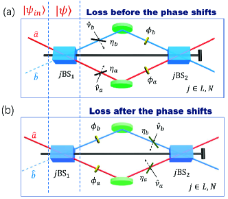
Figure 1: Lossy interferometer model. The losses in the interferometer are modeled by adding fictitious beam splitters (a) before and (b) after the phase shifts $\phi_{a}$ and $\phi_{b}$. The beam splitting is the passive linear beam splitters (LBSs) or the active nonlinear beam splitters (NBSs), corresponding the SU(2) interferometers or SU(1,1) interferometers, respectively. $\hat{v}_{a}$ ($\hat{v}_{b}$) is the vacuum, and $\eta_{a}$ ($\eta_{b}$) is transmission rate. In realistic systems the photon losses are distributed throughout the arms of the interferometer, not an event concentrated either before or after the phase, which is handled with a distribution parameter.

II QFIM of interferometers

II.1 Ideal QFIM

We consider a general interferometer, as shown in Fig. 1, where the beam splitter can be either linear or nonlinear, corresponding SU(2) and SU(1,1) interferometers, respectively. Consider the initial input state $|\psi_{in}\rangle$. After the first LBS or NBS, the state is labeled by $|\psi\rangle$. The two beams sustain phase shifts, i.e., mode $a$ undergoes a phase shift of $\phi_{a}$ and mode $b$ undergoes a phase shift of $\phi_{b}$, and the state is $\left|\psi_{\phi}\right\rangle$. Then the phase transformation is written as

$$\hat{U}_{\phi}^{ab}=\exp[i\phi_{a}\hat{n}_{a}+i\phi_{b}\hat{n}_{b}]=\exp(i\phi_{+}\hat{g}_{+})\exp(i\phi_{-}\hat{g}_{-}),$$ (1)

where $\phi_{\pm}=\phi_{a}\pm\phi_{b}$ and $g_{\pm}=(\hat{n}_{a}\pm\hat{n}_{b})/2$ with $\hat{n}_{a}=\hat{a}^{{\dagger}}\hat{a}$ and $\hat{n}_{b}=\hat{b}^{{\dagger}}\hat{b}$.

The QFI is the intrinsic information in the quantum state and is not related to the actual measurement procedure, which gives an upper limit to the precision of quantum parameter estimation. However, the QFI-only calculation was overestimated. In general, the phase estimation as a two-parameter estimation problem such as $\phi_{a}$ and $\phi_{b}$ (or $\phi_{+}$ and $\phi_{-}$), and the quantum Fisher information matrix (QFIM) is necessary.

In the SU(2) and SU(1,1) interferometers, the estimated phases are $\phi_{-}$ and $\phi_{+}$, respectively Kok2010 . For the estimation of $\phi_{+}$ and $\phi_{-}$ we can use the method of QFIM, which is given by a two-by-two matrix

$$\mathcal{F}_{QFIM}=\left[\begin{array}[]{cc}F_{++}&F_{+-}\\ F_{-+}&F_{--}\end{array}\right],$$ (2)

where $F_{ij}=4(\langle\hat{g}_{i}\hat{g}_{j}\rangle-\langle\hat{g}_{i}\rangle\langle\hat{g}_{j}\rangle)$ ($i$, $j=+,-$), $\langle\cdot\rangle$ denotes the average value $\left\langle\psi_{\phi}\right|\cdot|\psi_{\phi}\rangle$ as shown in Fig. 1. The estimation of $\phi_{-}$ and $\phi_{+}$ are respectively given by

$$\Delta^{2}\phi_{-}\geq\frac{1}{\mathcal{F}_{QFIM_{-}}}\text{, \ }\Delta^{2}\phi_{+}\geq\frac{1}{\mathcal{F}_{QFIM_{+}}},$$ (3)

where

$$\mathcal{F}_{QFIM_{-}} = F_{--}-\Delta F_{-}\text{, }\mathcal{F}_{QFIM_{+}}=F_{++}-\Delta F_{+},$$

$$\Delta\mathcal{F}_{-} = \frac{F_{+-}F_{-+}}{F_{++}}\text{, }\Delta\mathcal{F}_{+}=\frac{F_{+-}F_{-+}}{F_{--}}.$$ (4)

When $\Delta\mathcal{F}_{\pm}\neq 0$, $\Delta\mathcal{F}_{\pm}$ are the overestimated Fisher information from QFI-only calculation. If one ignores the nondiagonal terms, i.e., implicity assuming that $\phi_{+}$ ($\phi_{-}$) is known a priori, one could use the diagonal terms $F_{--}$ ($F_{++})$ to indicate the QFI of the single-parameter $\phi_{-}$ ($\phi_{+}$) estimation, where the misleading overestimates the precision limit Gong17 ; Takeoka ; You19 .

For a two-input-port interferometer, the matrix elements $F_{ij}$ are given by

$$F_{++} = \langle\Delta^{2}\hat{n}_{a}\rangle+\langle\Delta^{2}\hat{n}_{b}\rangle+2Cov[n_{a},n_{b}],$$

$$F_{--} = \langle\Delta^{2}\hat{n}_{a}\rangle+\langle\Delta^{2}\hat{n}_{b}\rangle-2Cov[n_{a},n_{b}],$$

$$F_{+-} = F_{-+}=\langle\Delta^{2}\hat{n}_{a}\rangle-\left\langle\Delta^{2}\hat{n}_{b}\right\rangle,$$ (5)

where $\langle\Delta^{2}\hat{n}_{i}\rangle=\langle\psi|\hat{n}_{i}^{2}|\psi\rangle-\langle\psi|\hat{n}_{i}|\psi\rangle^{2}$ $(i=a$, $b)$, and $Cov[\hat{n}_{a},\hat{n}_{b}]=\langle\psi|\hat{n}_{a}\hat{n}_{b}|\psi\rangle-\langle\psi|\hat{n}_{a}|\psi\rangle\langle\psi|\hat{n}_{b}|\psi\rangle$. $Cov[\hat{n}_{a},\hat{n}_{b}]$ is the covariance of two-mode field to describe the intermode correlation. After calculation, the ultimate $\mathcal{F}_{QFIM_{-}}$ and $\mathcal{F}_{QFIM_{+}}$ are rewritten as

$$\mathcal{F}_{QFIM_{-}} = 4\frac{\langle\Delta^{2}\hat{n}_{a}\rangle\langle\Delta^{2}\hat{n}_{b}\rangle-Cov[n_{a},n_{b}]^{2}}{\langle\Delta^{2}\hat{n}_{a}\rangle+\langle\Delta^{2}\hat{n}_{b}\rangle+2Cov[n_{a},n_{b}]},$$ (6)

$$\mathcal{F}_{QFIM_{+}} = 4\frac{\langle\Delta^{2}\hat{n}_{a}\rangle\langle\Delta^{2}\hat{n}_{b}\rangle-Cov[n_{a},n_{b}]^{2}}{\langle\Delta^{2}\hat{n}_{a}\rangle+\langle\Delta^{2}\hat{n}_{b}\rangle-2Cov[n_{a},n_{b}]}.$$ (7)

and the overestimated Fisher information are cast into

$$\Delta\mathcal{F}_{-} = \frac{\left(\langle\Delta^{2}\hat{n}_{a}\rangle-\langle\Delta^{2}\hat{n}_{b}\rangle\right)^{2}}{\langle\Delta^{2}\hat{n}_{a}\rangle+\langle\Delta^{2}\hat{n}_{b}\rangle+2Cov[n_{a},n_{b}]},$$ (8)

$$\Delta\mathcal{F}_{+} = \frac{\left(\langle\Delta^{2}\hat{n}_{a}\rangle-\langle\Delta^{2}\hat{n}_{b}\rangle\right)^{2}}{\langle\Delta^{2}\hat{n}_{a}\rangle+\langle\Delta^{2}\hat{n}_{b}\rangle-2Cov[n_{a},n_{b}]}.$$ (9)

This is a general expression, which is dependent on the form of the input state, and beam splitting transformation such as BS or NBS.

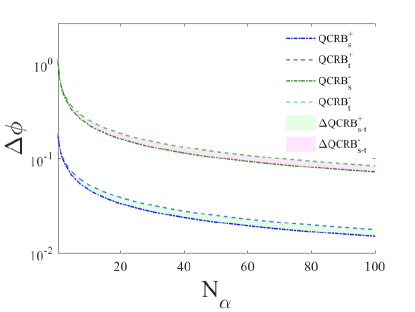
Figure 2: Phase sensitivity $\Delta\phi$ of SU(2) interferometers (top part) and SU(1,1) interferometers (bottom part) as a function of $N_{\alpha}$ with $r=1.5$, $T=0.7$, and $G_{1}=1.2$. QCRB${}^{k}_{p}$: $k\in$[+, SU(1,1) case; -, SU(2) case], $p\in$[s, QFI case; t, QFIM case]. The shaded parts represent the difference in phase sensitivities due to overestimated QFI.

Using the linear correlation coefficient $J$ to describe the intermode correlations Gerry05 , and the Mandel $Q$ parameter to describe the intramode Mandel95 , which are given by

$$J=\frac{Cov[\hat{n}_{a},\hat{n}_{b}]}{\langle\Delta\hat{n}_{a}\rangle\langle\Delta\hat{n}_{b}\rangle},\text{ }Q_{i}=\frac{\left\langle\Delta^{2}\hat{n}_{i}\right\rangle-\langle\hat{n}_{i}\rangle}{\langle\hat{n}_{i}\rangle},$$ (10)

where $\langle\Delta\hat{n}_{i}\rangle=\sqrt{\langle\Delta^{2}\hat{n}_{i}\rangle}$ $(i=a,b)$. Then, the ultimate $F_{QFIM_{-}}$ and $F_{QFIM_{+}}$ are rewritten as

$$\mathcal{F}_{QFIM_{-}} = \frac{4\sqrt{\left\langle\hat{n}_{a}\right\rangle\left\langle\hat{n}_{b}\right\rangle(Q_{a}+1)(Q_{b}+1)}(1-J^{2})}{\sqrt{\frac{\left\langle\hat{n}_{b}\right\rangle(Q_{b}+1)}{\left\langle\hat{n}_{a}\right\rangle(Q_{a}+1)}}+\sqrt{\frac{\left\langle\hat{n}_{a}\right\rangle(Q_{a}+1)}{\left\langle\hat{n}_{b}\right\rangle(Q_{b}+1)}}+2J},\text{ }\text{ }$$ (11)

$$\mathcal{F}_{QFIM_{+}} = \frac{4\sqrt{\left\langle\hat{n}_{a}\right\rangle\left\langle\hat{n}_{b}\right\rangle(Q_{a}+1)(Q_{b}+1)}(1-J^{2})}{\sqrt{\frac{\left\langle\hat{n}_{b}\right\rangle(Q_{b}+1)}{\left\langle\hat{n}_{a}\right\rangle(Q_{a}+1)}}+\sqrt{\frac{\left\langle\hat{n}_{a}\right\rangle(Q_{a}+1)}{\left\langle\hat{n}_{b}\right\rangle(Q_{b}+1)}}-2J}.\text{ }\text{ }$$ (12)

If $\langle\Delta^{2}\hat{n}_{a}\rangle=\langle\Delta^{2}\hat{n}_{b}\rangle$, the overestimated Fisher information $\Delta\mathcal{F}_{\pm}$ will be $0$, and the results of phase estimation $\phi_{\pm}$ are from the single-parameter QFI. Furthermore, considering $\left\langle\hat{n}_{a}\right\rangle=\left\langle\hat{n}_{b}\right\rangle=\bar{n}/2$, $\bar{n}$ is the average number of photons in the probe state, the results $\mathcal{F}_{QFIM_{\pm}}$ are reduced to

$$\mathcal{F}_{QFIM_{-}} = \mathcal{F}_{QFI_{-}}=\bar{n}(Q+1)(1-J),$$ (13)

$$\mathcal{F}_{QFIM_{+}} = \mathcal{F}_{QFI_{+}}=\bar{n}(Q+1)(1+J).$$ (14)

They are the same as that of the SU(2) Sahota15 and SU(1,1) Gong17 , respectively. The intermode correlation $J$ ranges between $-1$ and $1$, which contribute at most a factor of $2$ improvement in the QFI. The photon statistics within each arm of the interferometer are super-Poissonian and sub-Poissonian for $Q>0$ and $-1<Q<0$, respectively. Larger quantum enhancement originates from the photon variances within each arm of the interferometers Sahota15 ; Gong17 .

In the case of $\langle\Delta^{2}\hat{n}_{a}\rangle\neq\langle\Delta^{2}\hat{n}_{b}\rangle$, for the SU(2) interferometers it exists when the beam splitting ratio of the first LBS is not 50:50 without losses Jarzyna . However, in the presence of losses the optimal splitting ratio of LBS for the SU(2) interferometers is no longer 50:50, leading to $\langle\Delta^{2}\hat{n}_{a}\rangle\neq\langle\Delta^{2}\hat{n}_{b}\rangle$ Huang22 ; Cooper11 . For the SU(1, 1) interferometers, $\langle\Delta^{2}\hat{n}_{a}\rangle\neq\langle\Delta^{2}\hat{n}_{b}\rangle$ exists as long as that the input states of the two inputs are not the same Yu22 . Therefore, it is very necessary to estimate the phase sensitivity with noise by using the method of QFIM.

II.2 Lossy QFIM

In this section, the general model, developed by Escher et al. Escher11 for open quantum system metrology, is extended to the QFIM case.

We begin with a system $S$ and consider it along with the environment $E$. In general, the enlarged state of system and environment ($S+E$) evolves as

$$|\Psi\rangle_{SE}=\hat{U}_{SE}(x_{+},x_{-})|\psi\rangle_{S}|0\rangle_{E}=\sum_{l}\hat{\Pi}_{l}(x_{+},x_{-})|\psi\rangle_{S}|l\rangle_{E},$$ (15)

where $\hat{U}_{SE}(x_{+},x_{-})$ is the corresponding unitary operator, and $|\psi\rangle_{S}$ is the initial state of the probe. $|0\rangle_{E}$ is the initial state of the environment, and $|l\rangle_{E}$ are orthogonal states of the environment $E$. $\hat{\Pi}_{l}(x_{+},x_{-})$ are $x_{+}$, and $x_{-}$-dependent Kraus operators, which act on the system $S$. The evolution of an open system can be described as

$$\rho_{S} = Tr_{E}\left[\hat{U}_{SE}\rho_{SE}(0)\hat{U}_{SE}^{{\dagger}}\right]$$ (16)

$$= \sum_{l}\hat{\Pi}_{l}(x_{+},x_{-})|\psi\rangle_{SS}\langle\psi|\hat{\Pi}_{l}^{{\dagger}}(x_{+},x_{-}),$$

where $\rho_{SE}(0)$ is the state of the systems and environment. For the enlarged system-environment state, the QFI $\mathcal{C}_{QFIM}$ is given by

$$\mathcal{C}_{QFIM}=\left[\begin{array}[]{cc}C_{++}&C_{+-}\\ C_{-+}&C_{--}\end{array}\right],$$ (17)

where

$$C_{ij} = 4[\left\langle\psi\right|_{S}\left\langle l\right|_{E}\sum_{l}\frac{d\hat{\Pi}_{l}^{{\dagger}}(x_{+},x_{-})}{d\phi_{i}}\frac{d\hat{\Pi}_{l}(x_{+},x_{-})}{d\phi_{j}}\left|\psi\right\rangle_{S}\left|l\right\rangle_{E}$$

$$-\left\langle\psi\right|_{S}\left\langle l\right|_{E}\sum_{l}i\frac{d\hat{\Pi}_{l}^{{\dagger}}(x_{+},x_{-})}{d\phi_{i}}\hat{\Pi}_{l}(x_{+},x_{-})\left|\psi\right\rangle_{S}\left|l\right\rangle_{E}$$

$$\times\left\langle\psi\right|_{S}\left\langle l\right|_{E}\sum_{l}-i\hat{\Pi}_{l}^{{\dagger}}(x_{+},x_{-})\frac{d\hat{\Pi}_{l}(x_{+},x_{-})}{d\phi_{j}}\left|\psi\right\rangle_{S}\left|l\right\rangle_{E},$$

$$i,j \in (+,-).$$ (18)

The matrix elements $C_{ij}$ above can be expressed as

$$C_{ij} = 4[\left\langle\psi\right|_{S}\left\langle l\right|_{E}\hat{H}_{ij}(\phi_{+},\phi_{-})\left|\psi\right\rangle_{S}\left|l\right\rangle_{E}$$ (19)

$$-\left\langle\psi\right|_{S}\left\langle l\right|_{E}\hat{h}_{i}(\phi_{+},\phi_{-})\left|\psi\right\rangle_{S}\left|l\right\rangle_{E}$$

$$\times\left\langle\psi\right|_{S}\left\langle l\right|_{E}\hat{h}_{j}^{\prime}(\phi_{+},\phi_{-})\left|\psi\right\rangle_{S}\left|l\right\rangle_{E}],$$

where

$$\hat{H}_{ij}(\phi_{+},\phi_{-}) = \sum_{l}\frac{d\hat{\Pi}_{l}^{{\dagger}}(\phi_{+},\phi_{-})}{d\phi_{i}}\frac{d\hat{\Pi}_{l}(\phi_{+},\phi_{-})}{d\phi_{j}},$$

$$\hat{h}_{i}(\phi_{+},\phi_{-}) = i\sum_{l}\frac{d\hat{\Pi}_{l}^{{\dagger}}(\phi_{+},\phi_{-})}{d\phi_{i}}\hat{\Pi}_{l}(\phi_{+},\phi_{-}),$$

$$\hat{h}_{j}^{\prime}(\phi_{+},\phi_{-}) = -i\sum_{l}\hat{\Pi}_{l}^{{\dagger}}(\phi_{+},\phi_{-})\frac{d\hat{\Pi}_{l}(\phi_{+},\phi_{-})}{d\phi_{j}}.$$ (20)

By using QFIM method, similar to lossless case, we obtain the estimation of the phase difference $\phi_{-}$ and phase sum $\phi_{+}$ in the presence of losses, which is bounded by the QFIM:

$$\mathcal{C}_{QFIM_{-}} = C_{--}-\Delta C_{-},$$ (21)

$$\mathcal{C}_{QFIM_{+}} = C_{++}-\Delta C_{+},$$ (22)

where

$$\Delta C_{-}=\frac{C_{+-}C_{-+}}{C_{++}}\text{, }\Delta C_{+}=\frac{C_{+-}C_{-+}}{C_{--}}.$$ (23)

$\Delta C_{\pm}$ are the overestimated Fisher information from QFI-only calculation in the presence of losses. Because the additional freedom supplied by the environment should increase the QFI. Therefore, $\mathcal{C}_{QFIM_{+}}$ ($\mathcal{C}_{QFIM_{-}}$) should be larger or equal to $\mathcal{F}_{QFIM_{+}}$ ($\mathcal{F}_{QFIM_{-}}$) . The relation between $\mathcal{F}_{QFIM_{\pm}}$ and $\mathcal{C}_{QFIM_{\pm}}$ is found to be

$$\mathcal{F}_{QFIM_{i}} = \underset{\{\hat{\Pi}_{l}(x_{+},x_{-})\}}{\min}\mathcal{C}_{QFIM_{i}}\left[|\psi\rangle,\hat{\Pi}_{l}(x_{+},x_{-})\right],$$

$$i \in (+,-).$$ (24)

Usually, losses in the interferometers can be modeled by adding the fictitious beam splitters, and the lossy evolution of the field in two arms is described by the Kraus operator $\hat{\Pi}_{l}(\phi_{+},\phi_{-})$ with considering the phase shift. In realistic systems the photon losses are distributed throughout the arms of the interferometer, which is described by the parameter $\gamma$, instead of simply inserting the fictitious beam splitters before or after the phase shift.

Therefore, in the presence of losses the matrix elements of $\mathcal{F}_{QFIM_{\pm}}$ are worked in three steps: (1) substituting the $\hat{\Pi}_{l}(\phi_{+},\phi_{-})$ into Eq. (19), we can obtain the $C_{ij}$, which is a function of $\gamma$; (2) minimizing $\mathcal{C}_{QFIM_{\pm}}$ by the parameters $\gamma$, the optimal $\gamma_{opt}^{\pm}$ is obtained; (3) substituting $\gamma_{opt}^{\pm}$ into $\mathcal{C}_{QFIM_{\pm}}$, the minimum $\mathcal{C}_{QFIM_{\pm}}^{opt}$ is obtain, i.e., $\mathcal{F}_{QFIM_{\pm}}$ is achieved.

Next, we applied this model to analyze the phase estimation in the presence of losses in the case of in one arm and in two arms.

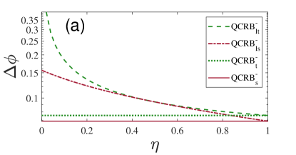
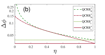
Figure 3: Phase sensitivities of (a) SU(2) interferometers and (b) SU(1,1) interferometers versus photon loss coefficient $\eta$ with single-parameter estimation and two-parameter estimation with $\left|\alpha\right|=10$, $r=0.5$ and $R/T=0.25$ in (a), $G_{1}=1.2$ in (b). QCRB${}^{k}_{p}$: $k\in$[+, SU(1,1) case; -, SU(2) case], $p\in$[s, QFI case; ls, QFI case with loss; t, QFIM case; lt, QFIM case with loss].

III Losses in one arm

Photon losses, a very usual noise, may happen at any stage of the phase process and is modeled by the fictitious LBS introduced in the interferometer arms. Firstly, we consider the photon losses in just one of the two arms, for example arm $a$. A possible set of Kraus operators describing the process without considering the phase shift is

$$\hat{\pi}_{l_{a}}=\sqrt{\frac{(1-\eta_{a})^{l_{a}}}{l_{a}!}}\eta_{a}^{\hat{n}_{a}/2}\hat{a}^{l_{a}},$$ (25)

where $\eta_{a}$ quantifies the photon losses of arm $a$ ($\eta_{a}=1$, lossless case; $\eta_{a}=0$, complete absorption).

When the photon losses before or after the phase shifts as shown in Fig. 1, the Kraus operators $\hat{\pi}_{l_{a}}(\phi_{+},\phi_{-})$ including the phase factor the general form ($\hbar=1$) is given by

$$\hat{\Pi}_{la}(\varphi_{+},\varphi_{-}) = \sqrt{\frac{(1-\eta_{a})^{l_{a}}}{l_{a}!}}e^{i\phi_{-}\frac{(\hat{a}^{\dagger}\hat{a}-\hat{b}^{\dagger}\hat{b}-\gamma l_{a})}{2}}$$ (26)

$$\times e^{i\phi_{+}\frac{(\hat{a}^{\dagger}\hat{a}+\hat{b}^{\dagger}\hat{b}-\gamma l_{a})}{2}}\eta_{a}^{\hat{n}_{a}/2}\hat{a}^{{}^{l_{a}}},$$

where $\gamma=0$ and $\gamma=-1$ describe the photons loss before and after the phase shifts, respectively.

According to Eqs. (20) and (26). The matrix elements $C_{ij}$ of Eq. (19) can be worked out:

$$C_{++} =\left[\eta_{a}+\gamma\eta_{a}-\gamma\right]^{2}\langle\Delta^{2}\hat{n}_{a}\rangle+\langle\Delta^{2}\hat{n}_{b}\rangle$$

$$+2\left[\eta_{a}+\gamma\eta_{a}-\gamma\right]Cov[\hat{n}_{a},\hat{n}_{b}]$$

$$+\left(\gamma+1\right)^{2}(1-\eta_{a})\eta_{a}\langle\hat{n}_{a}\rangle,$$ (27)

$$C_{--} =[\eta_{a}+\gamma\eta_{a}-\gamma]^{2}\langle\Delta^{2}\hat{n}_{a}\rangle+\langle\Delta^{2}\hat{n}_{b}\rangle$$

$$-2\left[\eta_{a}+\gamma\eta_{a}-\gamma\right]Cov[\hat{n}_{a},\hat{n}_{b}]$$

$$+\left(\gamma+1\right)^{2}(1-\eta_{a})\eta_{a}\left\langle\hat{n}_{a}\right\rangle,$$ (28)

$$C_{+-} =C_{-+}=[\eta_{a}+\gamma\eta_{a}-\gamma]^{2}\langle\Delta^{2}\hat{n}_{a}\rangle$$

$$+\left(\gamma+1\right)^{2}(1-\eta_{a})\eta_{a}\left\langle\hat{n}_{a}\right\rangle-\langle\Delta^{2}\hat{n}_{b}\rangle.$$ (29)

Substituting the matrix elements $C_{ij}$ into Eq. (21) and Eq. (22), one can obtain the $\mathcal{C}_{QFIM_{\pm}}$ for the case of loss in one arm, where $\mathcal{C}_{QFIM_{-}}$ and $\mathcal{C}_{QFIM_{+}}$ are SU(2) and SU(1,1) interferometers, respectively. They are given as follows:

$$\mathcal{C}_{QFIM_{-}} = 4\frac{\Upsilon_{0}}{\Upsilon_{1}+2J\Upsilon_{2}},$$ (30)

$$\text{ \ }\mathcal{C}_{QFIM+} = 4\frac{\Upsilon_{0}}{\Upsilon_{1}-2J\Upsilon_{2}},$$ (31)

where

$$\Upsilon_{0} = \left\langle\hat{n}_{a}\right\rangle\left\langle\hat{n}_{b}\right\rangle(Q_{b}+1)[\left(\gamma+1\right)^{2}(1-\eta_{a})\eta_{a}$$

$$+(\eta_{a}+\gamma\eta_{a}-\gamma)^{2}(1-J^{2})(Q_{a}+1)],$$

$$\Upsilon_{1} = \left\langle\hat{n}_{a}\right\rangle(Q_{a}+1)(\eta_{a}+\gamma\eta_{a}-\gamma)^{2}+\left\langle\hat{n}_{b}\right\rangle(Q_{b}+1)$$

$$+\left(\gamma+1\right)^{2}(1-\eta_{a})\eta_{a}\left\langle\hat{n}_{a}\right\rangle,$$

$$\Upsilon_{2} = \left\langle\hat{n}_{a}\right\rangle(Q_{a}+1)(\eta_{a}+\gamma\eta_{a}-\gamma)\sqrt{\frac{\left\langle\hat{n}_{b}\right\rangle(Q_{b}+1)}{\left\langle\hat{n}_{a}\right\rangle(Q_{a}+1)}}.\text{ \ }$$ (32)

Next, we minimize $\mathcal{C}_{QFIM_{\pm}}$ by varying parameter $\gamma$, respectively.

III.1 SU(2) interferometers

In the case of SU(2) interferometers. To minimize the $\mathcal{C}_{QFIM_{-}}$, it requires to find the optimal $\gamma$, and we get

$$\frac{d\mathcal{C}_{QFIM_{-}}}{d\gamma}=0.$$ (33)

After calculation, we obtain the optimal $\gamma_{opt}^{-}$, which is given by

$$\gamma_{opt}^{-}=\frac{1}{(1-\eta_{a})+\frac{\eta_{a}}{(Q_{a}+1)(1-J^{2})}(1+J\sqrt{\frac{\left\langle\hat{n}_{a}\right\rangle(Q_{a}+1)}{\left\langle\hat{n}_{b}\right\rangle(Q_{b}+1)}})}-1.$$ (34)

Substituting the optimal $\gamma_{opt}^{-}$ into $\mathcal{C}_{QFIM_{-}}$of Eq. (30), the optimal bound $\mathcal{C}_{QFIM_{-}}^{opt}$ is worked out:

$$\mathcal{C}_{QFIM_{-}}^{opt}=\frac{1}{\Upsilon_{3}}4(1-J^{2})[\langle\hat{n}_{a}\rangle\frac{\eta_{a}}{1-\eta_{a}}(1-J^{2})\left\langle\hat{n}_{b}\right\rangle(Q_{b}+1)$$

$$+\langle\hat{n}_{a}\rangle^{2}(\frac{\eta_{a}}{1-\eta_{a}})^{2}(\sqrt{\frac{\left\langle\hat{n}_{b}\right\rangle(Q_{b}+1)}{\left\langle\hat{n}_{a}\right\rangle(Q_{a}+1)}}+J)^{2}].$$ (35)

where

$$\Upsilon_{3} = (\frac{\eta_{a}\langle\hat{n}_{a}\rangle}{1-\eta_{a}})^{2}\{[\frac{1+5J^{2}}{\left\langle\hat{n}_{a}\right\rangle(Q_{a}+1)}+\frac{\left\langle\hat{n}_{b}\right\rangle(Q_{b}+1)}{\left\langle\hat{n}_{a}\right\rangle^{2}(Q_{a}+1)^{2}}$$ (36)

$$+\frac{J^{2}}{\left\langle\hat{n}_{b}\right\rangle(Q_{b}+1)}+\frac{2J(1+J^{2})}{\sqrt{\left\langle\hat{n}_{a}\right\rangle\left\langle\hat{n}_{b}\right\rangle(Q_{a}+1)(Q_{b}+1)}}$$

$$+\frac{4J}{\left\langle\hat{n}_{a}\right\rangle(Q_{a}+1)}\sqrt{\frac{\left\langle\hat{n}_{b}\right\rangle(Q_{b}+1)}{\left\langle\hat{n}_{a}\right\rangle(Q_{a}+1)}}]$$

$$+\langle\hat{n}_{a}\rangle\frac{\eta_{a}}{1-\eta_{a}}[(1-J^{2})[1+2\frac{\left\langle\hat{n}_{b}\right\rangle(Q_{b}+1)}{\left\langle\hat{n}_{a}\right\rangle(Q_{a}+1)}$$

$$+J^{2}+4J\sqrt{\frac{\left\langle\hat{n}_{b}\right\rangle(Q_{b}+1)}{\left\langle\hat{n}_{a}\right\rangle(Q_{a}+1)}}]\}$$

$$+(1-J^{2})^{2}\left\langle\hat{n}_{b}\right\rangle(Q_{b}+1).$$

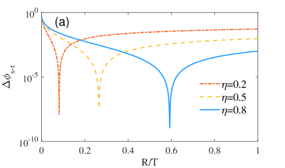
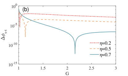
Figure 4: Phase sensitivity differences $\Delta\phi_{s-t}$ between the single-parameter estimation and the two-parameter estimation of (a) SU(2) interferometer versus $R/T$ and (b) SU(1,1) interferometer versus $G$ under the condition of different photon loss coefficient $\eta$, where $|\alpha|=2$, and $r=0.5$.

The bound $\mathcal{C}_{QFIM_{-}}^{opt}$ depends on the variance of the initial state $\left\langle\Delta^{2}\hat{n}_{a}\right\rangle$ and $\left\langle\Delta^{2}\hat{n}_{b}\right\rangle$, the number of photons in the initial state $\langle\hat{n}_{a}\rangle$, the intermode correlation $J$, and the losses $\eta_{a}$.

We check the optimal bound $\mathcal{C}_{QFIM_{-}}^{opt}$ in two limits. If there is small dissipation, that is

$$\langle\Delta^{2}\hat{n}_{b}\rangle,\langle\Delta^{2}\hat{n}_{a}\rangle\ll\langle\hat{n}_{a}\rangle\frac{\eta_{a}}{1-\eta_{a}}.$$ (37)

Eq. (35) arrives at

$$\mathcal{C}_{QFIM_{-}}^{opt} = \frac{1}{\Upsilon_{3L}}[4(1-J^{2})\left\langle\hat{n}_{a}\right\rangle(Q_{a}+1)$$ (38)

$$\times(\sqrt{\frac{\left\langle\hat{n}_{b}\right\rangle(Q_{b}+1)}{\left\langle\hat{n}_{a}\right\rangle(Q_{a}+1)}}+J)^{2}],$$

where

$$\Upsilon_{3L} = 1+J^{2}\frac{\left\langle\hat{n}_{a}\right\rangle(Q_{a}+1)}{\left\langle\hat{n}_{b}\right\rangle(Q_{b}+1)}+\frac{\left\langle\hat{n}_{b}\right\rangle(Q_{b}+1)}{\left\langle\hat{n}_{a}\right\rangle(Q_{a}+1)}$$ (39)

$$+2J(J^{2}+1)\sqrt{\frac{\left\langle\hat{n}_{a}\right\rangle(Q_{a}+1)}{\left\langle\hat{n}_{b}\right\rangle(Q_{b}+1)}}+5J^{2}$$

$$+4J\sqrt{\frac{\left\langle\hat{n}_{b}\right\rangle(Q_{b}+1)}{\left\langle\hat{n}_{a}\right\rangle(Q_{a}+1)}}.$$

When $\left\langle\hat{n}_{a}\right\rangle=\left\langle\hat{n}_{b}\right\rangle=\bar{n}/2$, and $\langle\Delta^{2}\hat{n}_{a}\rangle=\langle\Delta^{2}\hat{n}_{b}\rangle$, the overestimated Fisher information tends to $0$, then the result reduces to lossless case $F_{QFI_{-}}=\bar{n}(Q+1)(1-J)$ Sahota15 .

In the opposite, highly dissipative limit

$$\langle\Delta^{2}\hat{n}_{b}\rangle,\langle\Delta^{2}\hat{n}_{a}\rangle\gg\langle\hat{n}_{a}\rangle\frac{\eta_{a}}{1-\eta_{a}},$$ (40)

Eq. (35) is simplified as to

$$\mathcal{C}_{QFIM_{-}}^{opt}=\frac{\eta_{a}\langle\hat{n}_{a}\rangle}{1-\eta_{a}}(1-2J\frac{\langle\Delta\hat{n}_{b}\rangle}{\langle\Delta\hat{n}_{a}\rangle})-\Delta\mathcal{C}_{QFIM_{-}},$$ (41)

where the first term in $\mathcal{C}_{QFIM_{-}}$of Eq. (41) is the bound from the single-parameter estimation, which coincides with the bound by Escher et al. Escher11 and Demkowicz-Dobrzanski et al. Demkowicz . The second term $\Delta\mathcal{C}_{QFIM_{-}}$ is the overestimated Fisher information from QFI-only calculation in the presence of losses in the SU(2) interferometers, which is given by

$$\Delta\mathcal{C}_{QFIM_{-}}=\frac{over_{U}^{-}}{over_{D}^{-}},$$ (42)

where

$$over_{U}^{-} = \frac{\eta_{a}^{2}\langle\hat{n}_{a}\rangle^{2}}{(1-\eta_{a})^{2}}(1-2J\sqrt{\frac{\left\langle\hat{n}_{b}\right\rangle(Q_{b}+1)}{\left\langle\hat{n}_{a}\right\rangle(Q_{a}+1)}})$$

$$\times[1-J^{2}+2(J+\sqrt{\frac{\left\langle\hat{n}_{b}\right\rangle(Q_{b}+1)}{\left\langle\hat{n}_{a}\right\rangle(Q_{a}+1)}})^{2}]$$

$$-\frac{\eta_{a}\langle\hat{n}_{a}\rangle}{1-\eta_{a}}(1-J^{2})\left\langle\hat{n}_{b}\right\rangle(Q_{b}+1)$$

$$\times(2J\sqrt{\frac{\left\langle\hat{n}_{b}\right\rangle(Q_{b}+1)}{\left\langle\hat{n}_{a}\right\rangle(Q_{a}+1)}}+3),$$

$$over_{D}^{-} = \frac{\eta_{a}\langle\hat{n}_{a}\rangle}{1-\eta_{a}}[1-J^{2}+2(J+\sqrt{\frac{\left\langle\hat{n}_{b}\right\rangle(Q_{b}+1)}{\left\langle\hat{n}_{a}\right\rangle(Q_{a}+1)}})^{2}]$$ (43)

$$+(1-J^{2})\left\langle\hat{n}_{b}\right\rangle(Q_{b}+1).$$

When $\left\langle\hat{n}_{a}\right\rangle=\left\langle\hat{n}_{b}\right\rangle=\bar{n}/2$ and $\langle\Delta^{2}\hat{n}_{a}\rangle=\langle\Delta^{2}\hat{n}_{b}\rangle$, the overestimated Fisher information $\Delta\mathcal{C}_{QFIM_{-}}\neq 0$ in the presence of losses, it is different from lossless case.

III.2 SU(1,1) interferometers

In the case of SU(1, 1) interferometers. To minimize the $\mathcal{C}_{QFIM_{+}}$, it requires to find the optimal $\gamma$, and we obtain

$$\frac{d\mathcal{C}_{QFIM_{+}}}{d\gamma}=0.$$ (44)

Based on Eq. (44), the optimal $\gamma_{opt}^{+}$ is obtained

$$\gamma_{opt}^{+}=\frac{1}{(1-\eta_{a})+\frac{\eta_{a}}{(Q_{a}+1)(1-J^{2})}(1-J\sqrt{\frac{\left\langle\hat{n}_{a}\right\rangle(Q_{a}+1)}{\left\langle\hat{n}_{b}\right\rangle(Q_{b}+1)}})}-1.$$ (45)

Substituting the optimal $\gamma_{opt}^{+}$ into $\mathcal{C}_{QFIM_{+}}$ of Eq. (31), the optimal bound $\mathcal{C}_{QFIM_{+}}^{opt}$ is worked out:

$$\mathcal{C}_{QFIM_{+}}^{opt}=\frac{4}{\Upsilon_{4}}[\langle\hat{n}_{a}\rangle\frac{\eta_{a}}{1-\eta_{a}}(1-J^{2})^{2}\left\langle\hat{n}_{b}\right\rangle(Q_{b}+1)$$

$$+\langle\hat{n}_{a}\rangle^{2}(\frac{\eta_{a}}{1-\eta_{a}})^{2}(\sqrt{\frac{\left\langle\hat{n}_{b}\right\rangle(Q_{b}+1)}{\left\langle\hat{n}_{a}\right\rangle(Q_{a}+1)}}-J)^{2}(1-J^{2})],\text{ \ }$$ (46)

where

$$\Upsilon_{4} = (\frac{\eta_{a}\langle\hat{n}_{a}\rangle}{1-\eta_{a}})^{2}\{[\frac{1+5J^{2}}{\left\langle\hat{n}_{a}\right\rangle(Q_{a}+1)}+\frac{\left\langle\hat{n}_{b}\right\rangle(Q_{b}+1)}{\left\langle\hat{n}_{a}\right\rangle^{2}(Q_{a}+1)^{2}}$$ (47)

$$+\frac{J^{2}}{\left\langle\hat{n}_{b}\right\rangle(Q_{b}+1)}-\frac{2J(1+J^{2})}{\sqrt{\left\langle\hat{n}_{a}\right\rangle\left\langle\hat{n}_{b}\right\rangle(Q_{a}+1)(Q_{b}+1)}}$$

$$-\frac{4J}{\left\langle\hat{n}_{a}\right\rangle(Q_{a}+1)}\sqrt{\frac{\left\langle\hat{n}_{b}\right\rangle(Q_{b}+1)}{\left\langle\hat{n}_{a}\right\rangle(Q_{a}+1)}}]$$

$$+\langle\hat{n}_{a}\rangle\frac{\eta_{a}}{1-\eta_{a}}(1-J^{2})[1+2\frac{\left\langle\hat{n}_{b}\right\rangle(Q_{b}+1)}{\left\langle\hat{n}_{a}\right\rangle(Q_{a}+1)}$$

$$+J^{2}-4J\sqrt{\frac{\left\langle\hat{n}_{b}\right\rangle(Q_{b}+1)}{\left\langle\hat{n}_{a}\right\rangle(Q_{a}+1)}}]\}$$

$$+(1-J^{2})^{2}\left\langle\hat{n}_{b}\right\rangle(Q_{b}+1).$$

Similar to the SU(2) interferometers, we can also derive two limits. For small dissipation, that is

$$\langle\Delta^{2}\hat{n}_{b}\rangle,\langle\Delta^{2}\hat{n}_{a}\rangle\ll\langle\hat{n}_{a}\rangle\frac{\eta_{a}}{1-\eta_{a}}.$$ (48)

We get the reduced result

$$\mathcal{C}_{QFIM_{+}}^{opt}=4\frac{(\sqrt{\frac{\left\langle\hat{n}_{b}\right\rangle(Q_{b}+1)}{\left\langle\hat{n}_{a}\right\rangle(Q_{a}+1)}}-J)^{2}(1-J^{2})\left\langle\hat{n}_{a}\right\rangle(Q_{a}+1)}{\Upsilon_{4L}},$$ (49)

where

$$\Upsilon_{4L} = 1+5J^{2}+J^{2}\frac{\left\langle\hat{n}_{a}\right\rangle(Q_{a}+1)}{\left\langle\hat{n}_{b}\right\rangle(Q_{b}+1)}+\frac{\left\langle\hat{n}_{b}\right\rangle(Q_{b}+1)}{\left\langle\hat{n}_{a}\right\rangle(Q_{a}+1)}$$ (50)

$$-2J(1+J^{2})\sqrt{\frac{\left\langle\hat{n}_{a}\right\rangle(Q_{a}+1)}{\left\langle\hat{n}_{b}\right\rangle(Q_{b}+1)}}$$

$$-4J\sqrt{\frac{\left\langle\hat{n}_{b}\right\rangle(Q_{b}+1)}{\left\langle\hat{n}_{a}\right\rangle(Q_{a}+1)}}.$$

When $\left\langle\hat{n}_{a}\right\rangle=\left\langle\hat{n}_{b}\right\rangle=\bar{n}/2$, and $\langle\Delta^{2}\hat{n}_{a}\rangle=\langle\Delta^{2}\hat{n}_{b}\rangle$, the overestimated Fisher information tends to $0$, then the result reduces to lossless case $F_{QFI_{+}}=\bar{n}(Q+1)(1+J)$ Gong17 . Unlike the case of SU(2) interferometers, here is $1+J$ not $1-J$.

The highly dissipative limit is

$$\langle\Delta^{2}\hat{n}_{b}\rangle,\langle\Delta^{2}\hat{n}_{a}\rangle\gg\langle\hat{n}_{a}\rangle\frac{\eta_{a}}{1-\eta_{a}}.$$ (51)

we obtain

$$\mathcal{C}_{QFIM_{+}}^{opt}=\frac{\eta_{a}\langle\hat{n}_{a}\rangle}{1-\eta_{a}}(1+2J\frac{\langle\Delta\hat{n}_{b}\rangle}{\langle\Delta\hat{n}_{a}\rangle})-\Delta\mathcal{C}_{QFIM_{+}},$$ (52)

where

$$\Delta\mathcal{C}_{QFIM_{+}}=\frac{over_{U}^{+}}{over_{D}^{+}},$$ (53)

with

$$over_{U}^{+} = \frac{\eta_{a}^{2}\langle\hat{n}_{a}\rangle^{2}}{(1-\eta_{a})^{2}}(1+2J\sqrt{\frac{\left\langle\hat{n}_{b}\right\rangle(Q_{b}+1)}{\left\langle\hat{n}_{a}\right\rangle(Q_{a}+1)}})$$

$$\times[1-J^{2}+2(J-\sqrt{\frac{\left\langle\hat{n}_{b}\right\rangle(Q_{b}+1)}{\left\langle\hat{n}_{a}\right\rangle(Q_{a}+1)}})^{2}]$$

$$+\frac{\eta_{a}\langle\hat{n}_{a}\rangle}{1-\eta_{a}}(1-J^{2})\left\langle\hat{n}_{b}\right\rangle(Q_{b}+1)$$

$$\times(2J\sqrt{\frac{\left\langle\hat{n}_{b}\right\rangle(Q_{b}+1)}{\left\langle\hat{n}_{a}\right\rangle(Q_{a}+1)}}-3),$$

$$over_{D}^{+} = \frac{\eta_{a}\langle\hat{n}_{a}\rangle}{1-\eta_{a}}[1-J^{2}+2(J-\sqrt{\frac{\left\langle\hat{n}_{b}\right\rangle(Q_{b}+1)}{\left\langle\hat{n}_{a}\right\rangle(Q_{a}+1)}})^{2}]$$ (54)

$$+(1-J^{2})\left\langle\hat{n}_{b}\right\rangle(Q_{b}+1).$$

Similar to SU(2) interferometer case, when $\left\langle\hat{n}_{a}\right\rangle=\left\langle\hat{n}_{b}\right\rangle=\bar{n}/2$ and $\langle\Delta^{2}\hat{n}_{a}\rangle=\langle\Delta^{2}\hat{n}_{b}\rangle$, the overestimated Fisher information of $\Delta\mathcal{F}_{+}=0$ in lossless case becomes $\Delta\mathcal{C}_{QFIM_{-}}\neq 0$ in the presence of losses. Compare these two expressions $\Delta\mathcal{C}_{QFIM_{+}}$ and $\Delta\mathcal{C}_{QFIM-}$, there is only difference in signs between them. Since LBS and NBS are linear and nonlinear processes respectively, the average photon number and photon fluctuation of the same input state after LBS and NBS transformation will have significant differences, thus the phase sensitivity will also have significant differences.

IV Losses in two arms

Interferometers with photon losses in both arms as shown in Fig. 1 can be treated in a similar way. A possible set of Kraus operators describing the process is

$$\hat{\Pi}_{l_{a},l_{b}} =\sqrt{\frac{(1-\eta_{a})^{l_{a}}}{l_{a}!}}\sqrt{\frac{(1-\eta_{b})^{l_{b}}}{l_{b}!}}$$

$$\times e^{i\phi_{-}\frac{\hat{n}_{a}-\hat{n}_{b}-\gamma_{a}l_{a}+\gamma_{b}l_{b}}{2}} e^{i\phi_{+}\frac{\hat{n}_{a}+\hat{n}_{b}-\gamma_{a}l_{a}-\gamma_{b}l_{b}}{2}}\eta_{a}^{\frac{\hat{n}_{a}}{2}}\eta_{b}^{\frac{\hat{n}_{b}}{2}}\hat{a}^{l_{a}}\hat{b}^{l_{b}},$$ (55)

where $\eta_{a}$ ($\eta_{b}$) quantifies the photon losses of arm $a$ ($b$). $\gamma_{a}=-1$ and $\gamma_{b}=-1$ ($\gamma_{a}=0$ and $\gamma_{b}=0$) describe the photons loss before (after) the phase shifts of arm $a$ and arm $b$.

Substituting the $\hat{\Pi}_{l_{a},l_{b}}(\phi_{+},\phi_{-})$ into $C_{ij}$ of Eq. (19), the matrix elements $C_{ij}$ are given as follows:

$$C_{++}=[1-\Gamma_{a}(1-\eta_{a})]^{2}\left\langle\Delta\hat{n}_{a}^{2}\right\rangle+\Gamma_{a}^{2}(1-\eta_{a})\eta_{a}\left\langle\hat{n}_{a}\right\rangle$$

$$+[1-\Gamma_{b}(1-\eta_{b})]^{2}\left\langle\Delta\hat{n}_{b}^{2}\right\rangle+\Gamma_{b}^{2}(1-\eta_{b})\eta_{b}\left\langle\hat{n}_{b}\right\rangle$$

$$+2[1-\Gamma_{a}(1-\eta_{a})][1-\Gamma_{b}(1-\eta_{b})]Cov[\hat{n}_{a},\hat{n}_{b}],$$ (56)

$$C_{--}=[1-\Gamma_{a}(1-\eta_{a})]^{2}\left\langle\Delta\hat{n}_{a}^{2}\right\rangle+\Gamma_{a}^{2}(1-\eta_{a})\eta_{a}\left\langle\hat{n}_{a}\right\rangle$$

$$+[1-\Gamma_{b}(1-\eta_{b})]^{2}\left\langle\Delta\hat{n}_{b}^{2}\right\rangle+\Gamma_{b}^{2}(1-\eta_{b})\eta_{b}\left\langle\hat{n}_{b}\right\rangle$$

$$-2[1-\Gamma_{a}(1-\eta_{a})][1-\Gamma_{b}(1-\eta_{b})]Cov[\hat{n}_{a},\hat{n}_{b}],$$ (57)

$$C_{+-}=C_{-+}=[1-\Gamma_{a}(1-\eta_{a})]^{2}\left\langle\Delta\hat{n}_{a}^{2}\right\rangle+\Gamma_{a}^{2}(1-\eta_{a})\left\langle\hat{n}_{a}\right\rangle$$

$$\times\eta_{a}-[1-\Gamma_{b}(1-\eta_{b})]^{2}\left\langle\Delta\hat{n}_{b}^{2}\right\rangle-\Gamma_{b}^{2}(1-\eta_{b})\eta_{b}\left\langle\hat{n}_{b}\right\rangle,$$ (58)

where $\Gamma_{a}=\gamma_{a}+1$, $\Gamma_{b}=\gamma_{b}+1$.

Substituting the matrix elements $C_{ij}$ into $\mathcal{C}_{QFIM_{-}}$ of Eq. (21) and into $\mathcal{C}_{QFIM_{+}}$ of Eq. (22), we can obtain the $\mathcal{C}_{QFIM_{-}}$ and $\mathcal{C}_{QFIM_{+}}$. For convenience, considering $\gamma_{a}=\gamma_{b}=\gamma\equiv\Omega-1$, $\eta_{a}=\eta_{b}=\eta$, $\mathcal{C}_{QFIM_{-}}$ and $\mathcal{C}_{QFIM_{+}}$ are given by

$$\mathcal{C}_{QFIM_{-}}=4\frac{\Upsilon_{5}}{[1-\Omega(1-\eta)]_{-}^{2}\chi_{-}+\Omega^{2}(1-\eta)\eta\epsilon},$$ (59)

and

$$\mathcal{C}_{QFIM_{+}}=4\frac{\Upsilon_{5}}{[1-\Omega(1-\eta)]^{2}\chi_{+}+\Omega^{2}(1-\eta)\eta\epsilon},$$ (60)

where

$$\Upsilon_{5} = [1-\Omega(1-\eta)]^{4}\zeta+\Omega^{4}(1-\eta)^{2}\eta^{2}\tau$$ (61)

$$+[1-\Omega(1-\eta)]^{2}\Omega^{2}(1-\eta)\eta\lambda,$$

and

$$\chi_{\pm} = \left\langle\hat{n}_{a}\right\rangle(Q_{a}+1)+\left\langle\hat{n}_{b}\right\rangle(Q_{b}+1)$$

$$\mp 2J\sqrt{\left\langle\hat{n}_{a}\right\rangle\left\langle\hat{n}_{b}\right\rangle(Q_{a}+1)(Q_{b}+1)},$$

$$\zeta = (1-J^{2})\left\langle\hat{n}_{a}\right\rangle\left\langle\hat{n}_{b}\right\rangle(Q_{a}+1)(Q_{b}+1),$$

$$\epsilon = \left\langle\hat{n}_{a}\right\rangle+\left\langle\hat{n}_{b}\right\rangle,\tau=\left\langle\hat{n}_{a}\right\rangle\left\langle\hat{n}_{b}\right\rangle,$$

$$\lambda = \left\langle\hat{n}_{a}\right\rangle\left\langle\hat{n}_{b}\right\rangle\left[(Q_{a}+1)+(Q_{b}+1)\right].$$ (62)

Similar to single-arm loss case, we also minimize $\mathcal{C}_{QFIM_{-}}$ and $\mathcal{C}_{QFIM_{+}}$, corresponding to SU(2) and SU(1,1) interferometers, respectively.

IV.1 SU(2) interferometers

In the case of SU(2) interferometers. To minimize the $\mathcal{C}_{QFIM_{-}}$, it requires to find the optimal $\gamma$, and we get

$$\frac{d\mathcal{C}_{QFIM_{-}}}{d\gamma}=0.$$ (63)

The equation above is more complex, and we cannot obtain an analytical solution. Therefore, we check the $d\mathcal{C}_{QFIM_{-}}/d\gamma$ directly in two limits again. If there is small dissipation, we recover the QFIM $\mathcal{F}_{QFIM_{-}}$ for the lossless case.

In the opposite, if there is highly dissipative limit, due to high intensity we have $\left\langle\Delta\hat{n}_{b}^{2}\right\rangle_{0}\approx\left\langle\Delta\hat{n}_{a}^{2}\right\rangle_{0}$, and consider a special case $J=-1$ then we obtain the optimal $\gamma_{opt}^{H-}$, which is given by

$$\gamma_{opt}^{H-}=\frac{\eta\left[I-\tau\right]}{\left[\eta\tau+(1-\eta)\lambda\right]},$$ (64)

where the superscript $H$ indicates high loss. Substituting the optimal $\gamma_{opt}^{H-}$ into Eq. (22), the optimal bound $\mathcal{C}_{QFIM_{+}}^{H}$ is worked out:

$$\mathcal{C}_{QFIM_{-}}^{H}=4\frac{1}{(\Lambda_{-}^{H})^{2}\chi_{-}+(\Omega_{-}^{H})^{2}(1-\eta)\eta\epsilon}[(\Lambda_{-}^{H})^{4}\zeta$$

$$+(\Omega_{-}^{H})^{4}(1-\eta)^{2}\eta^{2}\tau+(\Lambda_{-}^{H})^{2}(\Omega_{-}^{H})^{2}(1-\eta)\eta\lambda],$$ (65)

where

$$\Omega_{-}^{H}=\frac{\lambda}{\left[\eta\tau+(1-\eta)\lambda\right]},\text{ }\Lambda_{-}^{H}=\frac{\eta\tau}{\left[\eta\tau+(1-\eta)\lambda\right]}.$$ (66)

IV.2 SU(1,1) interferometers

Substituting the matrix elements $C_{ij}$ into Eq. (21) and Eq. (22), ones can obtain the $\mathcal{C}_{QFIM_{-}}$ and $\mathcal{C}_{QFIM_{+}}$.

To minimize the $\mathcal{C}_{QFIM_{+}}$, it requires to find the optimal $\gamma$, and we obtain

$$\frac{d\mathcal{C}_{QFIM_{+}}}{d\gamma}=0.$$ (67)

Similar to the case of SU(2) interferometers, due to the above equation is more complex, we check the $d\mathcal{C}_{QFIM_{+}}/d\gamma$ directly in two limits again. If there is small dissipation, we recover the QFIM $\mathcal{F}_{QFIM+}$ for the lossless case.

In the opposite, if there is highly dissipative limit, due to high intensity we have $\left\langle\Delta\hat{n}_{b}^{2}\right\rangle_{0}\approx\left\langle\Delta\hat{n}_{a}^{2}\right\rangle_{0}$, and we also consider a special case $J=1$, we obtain the optimal $\gamma_{opt}^{H+}$, which is given by

$$\gamma_{opt}^{H+}=\frac{\eta\left[I-\tau\right]}{\left[\eta\tau+(1-\eta)\lambda\right]},$$ (68)

Substituting the optimal $\gamma_{opt}^{H+}$ into Eq. (22), the optimal bound $\mathcal{C}_{QFIM_{+}}^{H}$ is cast into:

$$\mathcal{C}_{QFIM_{+}}^{H}=4\frac{1}{(\Lambda_{+}^{H})^{2}\chi_{+}+(\Omega_{+}^{H})^{2}(1-\eta)\eta\epsilon}[(\Lambda_{+}^{H})^{4}\zeta$$

$$+(\Lambda_{+}^{H}\Omega_{+}^{H})^{2}(1-\eta)\eta\lambda+(\Omega_{+}^{H})^{4}(1-\eta)^{2}\eta^{2}\tau],$$ (69)

where

$$\Omega_{+}^{H}=\frac{\lambda}{\left[\eta\tau+(1-\eta)\lambda\right]},\text{ }\Lambda_{+}^{H}=\frac{\eta\tau}{\left[\eta\tau+(1-\eta)\lambda\right]}.$$ (70)

V QCRB and Numerical results

The phase sensitivity of the interferometer can be obtained for a given measurement scheme, such as homodyne measurement Li14 , parity measurement Li16 or intensity measurement Plick10 , with usage of error propagation formula. However, it is difficult to optimize over the detection methods to obtain the optimal estimation schemes. Fortunately, the QFI introduced by Braustein and Caves Braunstein94 ; Braunstein96 is the intrinsic information in the quantum state and is not related to a particular measurement scheme. Based on the QFI, the ultimate precision bound of phase sensitivity is given by the QCRB

$$\Delta\phi_{QCRB}=\frac{1}{\sqrt{m\mathcal{F}}},$$ (71)

where $m$ is the number of independent repeats of the experience.

Now we present a typical example to apply our theory to describe the difference between the QFI-only and QFIM. Here, We consider the case that the two input modes of the interferometer. We input the $\left|\alpha\right\rangle_{a}\otimes\left|\varsigma\right\rangle_{b}$, where coherent state $\left|\alpha\right\rangle$ with $\alpha=\left|\alpha\right|e^{i\theta_{\alpha}}$ with $\left|\alpha\right|$ being a complex number and $\theta_{\alpha}$ being the initial phase. And the squeezed vacuum state $\left|\varsigma\right\rangle=\exp[1/2(\varsigma^{\ast}\hat{a}^{2}-\varsigma(\hat{a}^{\dagger})^{2})$ with $\varsigma=re^{i\theta_{r}}$ is squeezed parameter where $r$ and $\theta_{r}$ are the squeezing amplitude and squeezing angle respectively.

V.1 SU(2) interferometers

In the SU(2) interferometer, the average number of photons in the two arms is $\langle\hat{n}_{a}\rangle^{-}=T\left|\alpha\right|^{2}+R\sinh^{2}r$ and $\langle\hat{n}_{b}\rangle^{-}=R\left|\alpha\right|^{2}+T\sinh^{2}r$, when $2\theta_{\alpha}-\theta_{r}=0$, we can get

$$\langle\Delta^{2}\hat{n}_{a}\rangle^{-} = T^{2}\left|\alpha\right|^{2}+2R^{2}\sinh^{2}r\cosh^{2}r$$

$$+TR(\left|\alpha\right|^{2}e^{2r}+\sinh^{2}r),$$

$$\langle\Delta^{2}\hat{n}_{b}\rangle^{-} = R^{2}\left|\alpha\right|^{2}+2T^{2}\sinh^{2}r\cosh^{2}r$$ (72)

$$+TR(\left|\alpha\right|^{2}e^{2r}+\sinh^{2}r),$$

and

$$Cov[\hat{n}_{a},\hat{n}_{b}]^{-}=TR(\left|\alpha\right|^{2}(1-e^{2r})+\sinh^{2}r\cosh 2r).$$ (73)

where $T$ and $R$ are the reflectivity and transmissivity of the BS, respectively. And using the above results one can get

$$Q_{a}^{-} = \frac{R(T\left|\alpha\right|^{2}(e^{2r}-1)+R\sinh^{2}r\cosh 2r)}{T\left|\alpha\right|^{2}+R\sinh^{2}r},$$

$$Q_{b}^{-} = \frac{T(R\left|\alpha\right|^{2}(e^{2r}-1)+T\sinh^{2}r\cosh 2r)}{R\left|\alpha\right|^{2}+T\sinh^{2}r}.$$

$$J^{-}=\frac{TR(\left|\alpha\right|^{2}(1-e^{2r})+\sinh^{2}r\cosh 2r)}{\sqrt{\begin{array}[]{c}\left[\begin{array}[]{c}T\left|\alpha\right|^{2}(T+Re^{2r})\\ +R\sinh^{2}r(T+2R\cosh^{2}r)\end{array}\right]\\ \times\left[\begin{array}[]{c}R\left|\alpha\right|^{2}(R+Te^{2r})\\ +T\sinh^{2}r(R+2T\cosh^{2}r)\end{array}\right]\end{array}}}.$$ (74)

V.2 SU(1,1) interferometers

Similar to the SU(2) interferometer case, we also consider the input $\left|\alpha\right\rangle_{a}\otimes\left|\varsigma\right\rangle_{b}$ in the SU(1,1) interferometer. The average number of photons in the two arms is $\langle\hat{n}_{a}\rangle^{+}=G^{2}\left|\alpha\right|^{2}+g^{2}\cosh^{2}r$ and $\langle\hat{n}_{b}\rangle^{+}=G^{2}\sinh^{2}r+g^{2}(\left|\alpha\right|^{2}+1)$, when $2\theta_{g}-2\theta_{\alpha}-\theta_{r}=\pi$, $\theta_{g}$ is the phase shift of the NBS for wave splitting and recombination. According to the above conditions, we obtain

$$\langle\Delta^{2}n_{a}\rangle^{+} = G^{4}\left|\alpha\right|^{2}+2g^{4}\sinh^{2}r\cosh^{2}r$$

$$+G^{2}g^{2}(\left|\alpha\right|^{2}e^{2r}+\cosh^{2}r),$$

$$\langle\Delta{}^{2}n_{b}\rangle^{+} = g^{4}\left|\alpha\right|^{2}+2G^{4}\sinh^{2}r\cosh^{2}r$$ (75)

$$+G^{2}g^{2}(\left|\alpha\right|^{2}e^{2r}+\cosh^{2}r),$$

and

$$Cov[\hat{n}_{a},\hat{n}_{b}]^{+}=G^{2}g^{2}(\left|\alpha\right|^{2}(1+e^{2r})+\cosh^{2}r\cosh 2r).$$ (76)

Here, $G$ is the gain factors of NBS, for wave splitting and recombination with $G^{2}-g^{2}=1$. The results are consistent with the results of Ref. You19 . Using the above results we work out

$$Q_{a}^{+} = \frac{g^{2}(G^{2}\left|\alpha\right|^{2}(1+e^{2r})+g^{2}\cosh^{2}r\cosh 2r)}{G^{2}\left|\alpha\right|^{2}+g^{2}\cosh^{2}r},$$

$$Q_{b}^{+} = \frac{\left[\begin{array}[]{c}G^{2}\sinh^{2}r\left[2G^{2}\cosh^{2}r+g^{2}-1\right]\\ +g^{2}(g^{2}(\left|\alpha\right|^{2}+1)+\left|\alpha\right|^{2}(G^{2}e^{2r}-1))\end{array}\right]}{G^{2}\sinh^{2}r+g^{2}(\left|\alpha\right|^{2}+1)}.$$ (79)

$$J^{+}=\frac{G^{2}g^{2}(\left|\alpha\right|^{2}(1+e^{2r})+\cosh^{2}r\cosh 2r)}{\sqrt{\begin{array}[]{c}\left[\begin{array}[]{c}G^{2}\left|\alpha\right|^{2}(G^{2}+g^{2}e^{2r})\\ +g^{2}\cosh^{2}r(G^{2}+2g^{2}\sinh^{2}r)\end{array}\right]\\ \times\left[\begin{array}[]{c}g^{2}\left|\alpha\right|^{2}(g^{2}+G^{2}e^{2r})\\ +G^{2}\cosh^{2}r(g^{2}+2G^{2}\sinh^{2}r)\end{array}\right]\end{array}}}.$$ (80)

Using the above results, we can obtain the numerical QCRBs in the case of losses in one arm and in two arms with the coherent state and squeezed vacuum state input for an example.

Firstly, we study the phase sensitivities of SU(1,1) interferometers or SU(2) interferometers and compare the differences between the results given by the QFI and QFIM phase estimation methods without loss. As shown in Fig. 2, the phase sensitivities of the SU(1,1) interferometer or SU(2) interferometer has difference between the single-parameter estimation and the two-parameter estimation under certain conditions. The difference is due to $\Delta F_{\pm}$ also known as overestimated Fisher Information. With the increase of $N_{\alpha}$, the difference of phase sensitivity caused by $\Delta F_{\pm}$ always exists, which corresponds to our conclusion in Sec. II.1. Therefore, it is appropriate to use the two-parameter estimation for the phase estimation of the interferometer.

Then, in the presence of loss of one arm, we study the phase sensitivities of SU(1,1) interferometers or SU(2) interferometers in the method of QFIM, as is depicted in Fig. 3. The QCRBs of the single-parameter estimation and the two-parameter estimation are very close, the sensitivity of them is approximately equal at moderate loss. In order to investigate this phenomenon, we study the difference of phase sensitivity $\Delta\phi_{s-t}$ between single-parameter and two-parameter estimation by changing $\eta$. In the case of SU(2) interferometers, $\Delta\phi_{s-t}$ as a function of $R/T$ under different photon loss coefficients $\eta$ is shown in Fig. 4(a). For a given $\eta$, there is a minimum value of $\Delta\phi_{s-t}$, which appears on the larger beam splitter ratio $R/T$ as $\eta$ increases. In the case of SU(1,1) ones, $\Delta\phi_{s-t}$ as a function of $G$ under different photon loss coefficients $\eta$ is shown in Fig. 4(b). Similar to the SU(2) case, there is also a minimum value of $\Delta\phi_{s-t}$, which appears on the larger $G$ as $\eta$ increases.

The overestimated Fisher Information in the ideal case gradually disappears as the loss increases. With the further increase of the loss, the overestimated Fisher Information reappears. The area of these minimum values of $\Delta\phi_{s-t}$ corresponds to $\Delta C_{\pm}=0$, i.e., $C_{+-}=C_{-+}=0$. Due to consider the single-arm loss (arm $a$), Eq. (29) can be written as $C_{+-}=C_{-+}=[\eta_{a}+\gamma\eta_{a}-\gamma]^{2}\langle\Delta^{2}\hat{n}_{a}\rangle+\left(\gamma+1\right)^{2}(1-\eta_{a})\eta_{a}\left\langle\hat{n}_{a}\right\rangle-\langle\Delta^{2}\hat{n}_{b}\rangle\equiv\overline{\langle\Delta^{2}\hat{n}_{a}\rangle}-\langle\Delta^{2}\hat{n}_{b}\rangle$, where $\overline{\langle\Delta^{2}\hat{n}_{a}\rangle}$ can be seen as effective fluctuation due to loss. Because the fluctuations $\overline{\langle\Delta^{2}\hat{n}_{a}\rangle}$ and $\langle\Delta^{2}\hat{n}_{b}\rangle$ are different, when the loss increases gradually, $\overline{\langle\Delta^{2}\hat{n}_{a}\rangle}$ decreases gradually. When it decreases to the same as the other arm, the overestimated Fisher Information disappears. The loss continues to increase, and the fluctuation $\overline{\langle\Delta^{2}\hat{n}_{a}\rangle}$ in turn continues to increase, leading to the re-emergence of overestimation. A similar phenomenon also occurs in the loss of both arms.

VI conclusion

In conclusion, we theoretically extended the model developed by Escher et al Escher11 to the QFIM case with noise. Photon loss is a very usual noise in optical systems, then we gave the QFIM expressions in the case of single-arm photon loss and two-arm photon losses in the SU(2) and SU(1,1) interferometers with arbitrary pure states input. The ultimate precision limits of SU(2) and SU(1,1) interferometers with photon losses was investigated and discussed by using coherent state $\otimes$ squeezed vacuum state as an example. The overestimated Fisher Information existing in the ideal case will occur disappear and revival phenomenon with loss coefficient or splitter ratio changing. For a given loss coefficient, adjusting the splitter ratio is a method to optimize the sensitivity of quantum measurements in a lossy environment. This strategy is beneficial to quantum precision measurement in lossy environments.

VII Acknowledgments

This work is supported by the National Natural Science Foundation of China Grants No. 11974111, No. 11874152, No. 12104423, No. 11654005, No. 11974116, No. 91536114, Shanghai Municipal Science and Technology Major Project under Grant No. 2019SHZDZX01; Innovation Program of Shanghai Municipal Education Commission No. 202101070008E00099; the Fundamental Research Funds for the Central Universities; the Shanghai talent program.

References

• (1) C. W. Helstrom, Quantum Detection and Estimation Theory (Academic, New York, 1976).
• (2) A. S. Holevo, Probabilistic and Statistical Aspects of Quantum Theory (North-Holland, Amsterdam, 1982).
• (3) C. M. Caves, Quantum-mechanical noise in an interferometer, Phys. Rev. D 23, 1693(1981)
• (4) S. L. Braunstein and C. M. Caves, Statistical distance and the geometry of quantum states, Phys. Rev. Lett. 72, 3439 (1994).
• (5) S. L. Braunstein, C. M. Caves, and G. J. Milburn, Generalized uncertainty relations: Theory, examples, and Lorentz invariance, Ann. Phys. 247, 135 (1996).
• (6) H. Lee, P. Kok, and J. P. Dowling, J Mod, A quantum Rosetta stone for interferometry, Opt 49, 2325 (2002).
• (7) V. Giovannetti, S. Lloyd, and L. Maccone, Quantum Metrology, Phys. Rev. Lett. 96, 010401 (2006).
• (8) M. Zwierz, C. A. Pérez-Delgado, and P. Kok, General Optimality of the Heisenberg Limit for Quantum Metrology, Phys. Rev. Lett. 105, 180402 (2010).
• (9) V. Giovannetti, S. Lloyd, and L. Maccone, Quantum-Enhanced Measurements: Beating the Standard Quantum Limit, Science 306, 1330 (2004).
• (10) V. Giovannetti, S. Lloyd, and L. Maccone, Advances in quantum metrology, Nature photonics 5, 222 (2011).
• (11) B. Yurke, S. L. McCall, and J. R. Klauder, SU(2) and SU(1 1) interferometers, Phys. Rev. A 33, 4033 (1986).
• (12) J. Jing, C. Liu, Z. Zhou, Z. Y. Ou, and W. Zhang, Realization of a nonlinear interferometer with parametric amplifiers, Appl. Phys. Lett. 99, 011110 (2011).
• (13) F. Hudelist, J. Kong, C. Liu, J. Jing, Z. Y. Ou, and W. Zhang, Quantum metrology with parametric amplifier-based photon correlation interferometers, Nat. Commun. 5, 3049 (2014).
• (14) B. Chen, C. Qiu, S. Chen, J. Guo, L. Q. Chen, Z. Y. Ou, and W. Zhang, Atom-Light Hybrid Interferometer, Phys. Rev. Lett. 115, 043602 (2015).
• (15) C. Qiu, S. Chen, L. Q. Chen, B. Chen, J. Guo, Z. Y. Ou, and W. Zhang, Atom–light superposition oscillation and Ramsey-like atom–light interferometer, Optica 3, 775 (2016).
• (16) D. Linnemann, H. Strobel, W. Muessel, J. Schulz, R. J. Lewis-Swan, K. V. Kheruntsyan, and M. K. Oberthaler, Quantum-Enhanced Sensing Based on Time Reversal of Nonlinear Dynamics, Phys. Rev. Lett. 117, 013001 (2016).
• (17) S. Lemieux, M. Manceau, P. R. Sharapova, O. V. Tikhonova, R. W. Boyd, G. Leuchs, and M. V. Chekhova, Engineering the Frequency Spectrum of Bright Squeezed Vacuum via Group Velocity Dispersion in an SU(1,1) Interferometer, Phys. Rev. Lett. 117, 183601 (2016).
• (18) M. Manceau, G. Leuchs, F. Khalili, and M. Chekhova, Detection Loss Tolerant Supersensitive Phase Measurement with an SU(1,1) Interferometer, Phys. Rev. Lett. 119, 223604 (2017).
• (19) B. E. Anderson, P. Gupta, B. L. Schmittberger, T. Horrom, C. Hermann-Avigliano, K. M. Jones, and P. D. Lett, Phase sensing beyond the standard quantum limit with a variation on the SU(1,1) interferometer, Optica 4, 752 (2017).
• (20) P. Gupta, B. L. Schmittberger, B. E. Anderson, K. M. Jones, and P. D. Lett, Optimized phase sensing in a truncated SU(1,1) interferometer, Opt. Express 26, 000391 (2017).
• (21) W. Du, J. Jia, J. F. Chen, Z. Y. Ou, and W. Zhang, Absolute sensitivity of phase measurement in an SU(1,1) type interferometer, Opt. Lett. 43, 1051 (2018).
• (22) G. Frascella, E. E. Mikhailov, N. Takanashi, R.V. Zakharov, O.V. Tikhonova, M. V. Chekhova, Wide-field SU(1,1) interferometer, Optica 6, 1233 (2019).
• (23) N. Prajapati, I. Novikova, Polarization-based truncated SU(1,1) interferometer based on four-wave mixing in Rb vapor, Opt. Lett. 44, 5921 (2019).
• (24) W. Du, J. Kong, G. Bao, P. Yang, J. Jia, S. Ming, C.-H. Yuan, J. F. Chen, Z. Y. Ou, M. W. Mitchell, and W. Zhang, SU(2)-in-SU(1,1) Nested Interferometer for High Sensitivity, Loss-Tolerant Quantum Metrology, Phys. Rev. Lett. 128, 033601 (2022).
• (25) W. N. Plick, J. P. Dowling, and G. S. Agarwal, Coherent-light-boosted, sub-shot noise, quantum interferometry, New J. Phys. 12, 083014 (2010).
• (26) Z. Y. Ou, Enhancement of the phase-measurement sensitivity beyond the standard quantum limit by a nonlinear interferometer, Phys. Rev. A 85, 023815 (2012).
• (27) A. M. Marino, N. V. Corzo Trejo, and P. D. Lett, Effect of losses on the performance of an SU(1,1) interferometer, Phys. Rev. A 86, 023844 (2012).
• (28) D. Li, C.-H. Yuan, Z. Y. Ou, and W. Zhang, The phase sensitivity of an SU (1,1) interferometer with coherent and squeezed-vacuum light, New J. Phys. 16, 073020 (2014).
• (29) H. Ma, D. Li, C.-H. Yuan, L. Q. Chen, Z. Y. Ou, and W. Zhang, SU(1,1)-type light-atom-correlated interferometer, Physical Review A 92, 023847 (2015).
• (30) M. Gabbrielli, L. Pezzè, and A. Smerzi, Spin-Mixing Interferometry with Bose-Einstein Condensates, Phys. Rev. Lett. 115, 163002 (2015).
• (31) Z.-D. Chen, C.-H. Yuan, H.-M. Ma, D. Li, L. Q. Chen, Z. Y. Ou, and W. Zhang, Effects of losses in the atom-light hybrid SU(1,1) interferometer, Opt. Express 24, 17766 (2016).
• (32) C. Sparaciari, S. Olivares, and M. G. A. Paris, Gaussian-state interferometry with passive and active elements, Phys. Rev. A 93, 023810 (2016).
• (33) D. Li, B. T. Gard, Y. Gao, C.-H. Yuan, W. Zhang, H. Lee, and J. P. Dowling, Phase sensitivity at the Heisenberg limit in an SU(1,1) interferometer via parity detection, Phys. Rev. A 94, 063840 (2016).
• (34) X. Y. Hu, C. P. Wei, Y. F. Yu, Z. M. Zhang, Enhanced phase sensitivity of an SU(1,1) interferometer with displaced squeezed vacuum light, Front. Phys. 11, 114203 (2016).
• (35) Q.-K. Gong, X.-L. Hu, D. Li, C.-H. Yuan, Z. Y. Ou, and W. Zhang, Intramode correlations enhanced phase sensitivities in an SU(1,1) interferometer, Physical Review A 96, 033809 (2017).
• (36) E. Giese, S. Lemieux, M. Manceau, R. Fickler, and R.W. Boyd, Phase sensitivity of gain-unbalanced nonlinear interferometers, Phys. Rev. A 96, 053863 (2017).
• (37) D. Li, C.-H. Yuan, Y. Yao, W. Jiang, M. Li, and W. Zhang, Effects of loss on the phase sensitivity with parity detection in an SU(1,1) interferometer, J. Opt. Soc. Am. B 35, 1080 (2018).
• (38) L. L. Guo, Y. F. Yu, Z. M. Zhang, Improving the phase sensitivity of an SU(1,1) interferometer with photon-added squeezed vacuum light, Opt. Express 26, 29099 (2018).
• (39) X. P. Ma, C. L. You, S. Adhikari, E. S. Matekole, R. T. Glasser, H. Lee, J. P. Dowling, Sub-shot-noise-limited phase estimation via SU(1,1) interferometer with thermal states. Opt. Express 26, 18492 (2018).
• (40) X.-L. Hu, D. Li, L. Q. Chen, K. Zhang, W. Zhang, and C.-H. Yuan, Phase estimation for an SU(1,1) interferometer in the presence of phase diffusion and photon losses, Phys. Rev. A 98, 023803 (2018).
• (41) Y. Michael, L. Bello, M. Rosenbluh, and A. Pe’er, Squeezing-enhanced Raman spectroscopy, npj Quantum Inf 5, 81 (2019).
• (42) G.-F. Jiao, K. Zhang, L. Q. Chen, W. Zhang, and C.-H. Yuan, The nonlinear phase estimation enhanced by an actively correlated Mach-Zehnder interferometer, Physical Review A 102, 033520 (2020).
• (43) Z.Y. Ou, X.Y. Li, Quantum SU(1,1) interferometers: Basic principles and applications, APL Photonics 5, 080902 (2020).
• (44) G.-F. Jiao, K. Zhang, L. Q. Chen, C.-H. Yuan, and W. Zhang, Quantum non-demolition measurement based on an SU(1,1)-SU(2)-concatenated atom–light hybrid interferometer, Photon. Res. 10, 475 (2022).
• (45) X. Liang, Zhifei Yu, Chun-Hua Yuan, Weiping Zhang and Liqing Chen, Phase sensitivity improvement in correlation-enhanced nonlinear interferometers, Symmetry 14, 02684 (2022)
• (46) R. Demkowicz-Dobrzanski, U. Dorner, B. J. Smith, J. S. Lundeen, W. Wasilewski, K. Banaszek, and I. A. Walmsley, Quantum phase estimation with lossy interferometers, Phys. Rev. A 80, 013825 (2009).
• (47) B. M. Escher, R. L. de Matos Filho, L. Davidovich, General framework for estimating the ultimate precision limit in noisy quantum-enhanced metrology, Nature Phys. 7, 406 (2011).
• (48) R. Demkowicz-Dobrzanski, J. Kolodynski, and M. Guta, The elusive Heisenberg limit in quantum-enhanced metrology, Nat. Commun. 3, 1063 (2012).
• (49) J.-D. Yue, Y.-R. Zhang, and H. Fan, Quantum-enhanced metrology for multiple phase estimation with noise. Sci. Rep. 4, 5933 (2014).
• (50) D. W. Berry, Michael J. W. Hall, and H. M. Wiseman, Stochastic Heisenberg Limit: Optimal Estimation of a Fluctuating Phase, Phys. Rev. Lett. 111, 113601 (2013).
• (51) R. Chaves, J. B. Brask, M. Markiewicz, J. Kołodynski, and A. Acin, Noisy Metrology beyond the Standard Quantum Limit, Phys. Rev. Lett. 111, 120401 (2013).
• (52) W. Dur, M. Skotiniotis, F. Frowis, and B. Kraus, Improved Quantum Metrology Using Quantum Error Correction, Phys. Rev. Lett. 112, 080801 (2014).
• (53) E. M. Kessler, I. Lovchinsky, A. O. Sushkov, and M. D. Lukin, Quantum Error Correction for Metrology, Phys. Rev. Lett. 112, 150802 (2014).
• (54) D. Brivio, S. Cialdi, S. Vezzoli, B. T. Gebrehiwot, M. G. Genoni, S. Olivares, and M. G. A. Paris, Experimental estimation of one-parameter qubit gates in the presence of phase diffusion, Phys. Rev. A 81, 012305(2010).
• (55) S. Alipour, M. Mehboudi, and A. T. Rezakhani, Quantum Metrology in Open Systems: Dissipative Cramer-Rao Bound, Phys. Rev. Lett. 112, 120405 (2014).
• (56) B. M. Escher, L. Davidovich, N. Zagury, and R. L. de Matos Filho, Quantum Metrological limits via a variational approach, Phys. Rev. Lett. 109, 190404 (2012).
• (57) M. G. Genoni, S. Olivares, and M. G. A. Paris, Opical Phase Estimation in the Presence of Phase Diffusion, Phys. Rev. Lett. 106, 153603 (2011).
• (58) M. G. Genoni, S. Olivares, D. Brivio, S. Cialdi, D. Cipriani, A. Santamato, S. Vezzoli, and M. G. A. Paris, Opical interferometry in the presence of large phase diffusin, Phys. Rev. A 85, 043817 (2012).
• (59) X. M. Feng, G. R. Jin, and W. Yang, Quantum interferometry with binary-outcome measurements in the presence of phase diffusion, Phys. Rev. A 90, 013807 (2014).
• (60) G. Toth and I. Apellaniz, Quantum metrology from a quantum information science perspective, J. Phys. A 47, 424006 (2014).
• (61) L. Pezzè and A. Smerzi, in Proceedings of the International School of Physics “Enrico Fermi”, Course CLXXXVIII “Atom Interferometry” edited by G. Tino and M. Kasevich (Società Italiana di Fisica and IOS Press, Bologna, 2014), p. 691.
• (62) R. Demkowicz-Dobrzanski, M. Jarzyna, J. Kolodynski, Quantum limits in optical interferometry, Progress in Optics 60, 345 (2015).
• (63) X.-B. Wang, T. Hiroshima, A. Tomita, M. Hayashi, Quantum information with Gaussian states, Opt. Reports 448, 1 (2007).
• (64) C. Sparaciari, S. Olivares, and M. G. A. Paris, Bounds to precision for quantum interferometry with Gaussian states and operations, J. Opt. Soc. Am. B 32, 1354 (2015).
• (65) A. Monras, Phase space formalism for quantum estimation of Gaussian states, arXiv:1303.3682v1 (2013).
• (66) O. Pinel, P. Jian, N. Treps, C. Fabre, and D. Braun, Quantum parameter estimation using general single-mode Gaussian states, Phys. Rev. A 88, 040102(R) (2013).
• (67) J. Liu, X. Jing, and X. Wang, Phase-matching condition for enhancement of phase sensitivity in quantum metrology, Phys. Rev. A 88, 042316 (2013).
• (68) Y. Gao and H. Lee, Bounds on quantum multiple-parameter estimation with Gaussian state, Eur. Phys. J. D 68, 347 (2014).
• (69) Z. Jiang, Quantum Fisher information for states in exponential form, Phys. Rev. A 89, 032128 (2014).
• (70) D. Safranek, A. R. Lee, and I. Fuentes, Quantum parameter estimation using multi-mode Gaussian states, New J. Phys. 17, 073016 (2015).
• (71) G.-F. Jiao, Q. Wang, Z. Yu, L. Q. Chen, W. Zhang, and C.-H. Yuan, Effects of losses on the sensitivity of an actively correlated Mach-Zehnder interferometer, Physical Review A 104, 013725 (2021).
• (72) S. Chang, W. Ye, X. Rao, J. Wen, H. Zhang, Q. Gong, L. Huang, M. Luo, Y. Chen, L. Hu, and S. Gao, Intramode-correlation–enhanced simultaneous multiparameter-estimation precision, Phys. Rev. A 106, 062409 (2022).
• (73) M. Jarzyna and R. Demkowicz-Dorbrzanski, Quantum interferometry with and without an external phase reference, Phys. Rev. A 85, 011801(R) (2012).
• (74) Q. K. Gong, D. Li, C. H. Yuan, Z. Y. Ou, and W. P. Zhang, Chinese Phys. B 26, 094205 (2017).
• (75) C. You, S. Adhikari, X. Ma, M. Sasaki, M. Takeoka, and J. P. Dowling, Conclusive precision bounds for SU(1,1) interferometers, Phys. Rev. A 99, 042122 (2019).
• (76) M. Takeoka, K. P. Seshadreesan, C. You, S. Izumi, and J. P. Dowling, Fundamental precision limit of a Mach-Zehnder interferometric sensor when one of the inputs is the vacuum, Phys. Rev. A 96, 052118 (2017).
• (77) M. D. Lang and C. M. Caves, Optimal Quantum-Enhanced Interferometry Using a Laser Power Source, Phys. Rev. Lett. 111, 173601 (2013).
• (78) M. D. Lang and C. M. Caves, Optimal quantum-enhanced interferometry, Phys. Rev. A 90, 025802 (2014).
• (79) S. Ataman, A. Preda, and R. Ionicioiu, Phase sensitivity of a Mach-Zehnder interferometer with single-intensity and difference-intensity detection, Phys. Rev. A 98, 043856 (2018).
• (80) W. Zhong, F. Wang, L. Zhou, P. Xu, and Y. Sheng, Quantum-enhanced interferometry with asymmetric beam splitters, Sci. China Phys. Mech. Astron. 63, 260312 (2020).
• (81) P. Kok and B. W. Lovett, Introduction to Optical Quantum Information Processing (Cambridge University Press, 2010), Chap. 13.
• (82) C. C. Gerry and P. L. Knight, Introductory Quantum Optics (Cambridge University Press, Cambridge, 2005).
• (83) L. Mandel and E. Wolf, Optical Optical coherent and quantum optics (Cambridge University Press, Cambridge, 1955).
• (84) J. Sahota and N. Quesada, Quantum correlations in optical metrology: Heisenberg-limited phase estimation without mode entanglement, Phys. Rev. A 91, 013808 (2015).
• (85) W. Huang, X. Liang, B. Zhu, Y. Yan, C.-H. Yuan, W. Zhang, and L. Q. Chen, Protection of noise squeezing in a quantum interferometer with optimal resource allocation, Phys. Rev. Lett., in press (2023).
• (86) J. J. Cooper and J. A. Dunningham, Towards improved interferometric sensitivities in the presence of loss, New J. Phys. 13, 115003 (2011).
• (87) Z. Yu, B. Fang, P. Liu, S. Chen, G. Bao, C.-H. Yuan, and L. Q. Chen, Sensing performance enhancement via asymmetric gain optimization in the atom-light hybrid interferometer, Opt. Express 30, 11514 (2022).