Compressing Tabular Data via Latent Variable Estimation

Compressing Tabular Data via Latent Variable Estimation

Abstract

Data used for analytics and machine learning often take the form of tables with categorical entries. We introduce a family of lossless compression algorithms for such data that proceed in four steps: $(i)$ Estimate latent variables associated to rows and columns; $(ii)$ Partition the table in blocks according to the row/column latents; $(iii)$ Apply a sequential (e.g. Lempel-Ziv) coder to each of the blocks; $(iv)$ Append a compressed encoding of the latents.

We evaluate it on several benchmark datasets, and study optimal compression in a probabilistic model for that tabular data, whereby latent values are independent and table entries are conditionally independent given the latent values. We prove that the model has a well defined entropy rate and satisfies an asymptotic equipartition property. We also prove that classical compression schemes such as Lempel-Ziv and finite-state encoders do not achieve this rate. On the other hand, the latent estimation strategy outlined above achieves the optimal rate.

1 Introduction

Classical theory of lossless compression [CT06, Sal04] assumes that data take the form of a random vector $\boldsymbol{X}^{N}=(X_{1},X_{2},\dots,X_{N})$ of length $N$ with entries in a finite alphabet ${\mathcal{X}}$. Under suitable ergodicity assumptions, the entropy per letter converges to a limit $h:=\lim_{N\to\infty}H(\boldsymbol{X}^{N})/N$ (Shannon-McMillan-Breiman theorem). Universal coding schemes (e.g. Lempel-Ziv coding) do not requite knowledge of the distribution of $\boldsymbol{X}^{N}$, and can encode such a sequence without information loss using (asymptotically) $h$ bits per symbol.

While this theory is mathematically satisfying, its modeling assumptions (stationarity, ergodicity) are unlikely to be satisfied in many applications. This has long been recognized by practitioners. The main objective of this paper is to investigate this fact mathematically in the context of tabular data, characterize the gap to optimality of classical schemes, and describe an asymptotically optimal algorithm that overcomes their limitations.

We consider a data table with $m$ rows and $n$ columns and entries in ${\mathcal{X}}$, $\boldsymbol{X}^{m,n}\in{\mathcal{X}}^{m\times n}$ $\boldsymbol{X}^{m,n}:=(X_{ij})_{i\leq m,j\leq n}$. The standard approach to such data is: $(i)$ Serialize, e.g. in row-first order, to form a vector of length $N=mn$, $\boldsymbol{X}^{N}=(X_{11},X_{12},\dots,X_{1n},X_{21},\dots,X_{mn})$; $(ii)$ Apply a standard compressor (e.g., Lempel-Ziv) to this vector.

We will show, both empirically and mathematically that this standard approach can be suboptimal in the sense of not achieving the optimal compression rate. This happens even in the limit of large tables, as long as the number of columns and rows are polynomially related (i.e. $n^{{\varepsilon}}\leq m\leq n^{M}$ for some small constant ${\varepsilon}$ and large constant $M$).

We advocate an alternative approach:

1. Estimate row/column latents ${\boldsymbol{u}}^{m}=(u_{1},\dots,u_{m})\in{\cal L}^{m}$, ${\boldsymbol{v}}^{n}=(v_{1},\dots,v_{n})\in{\cal L}^{n}$, with ${\cal L}$ a finite alphabet.

2. Partition the table in blocks according to the row/column latents, Namely, for $u,v\in{\cal L}$, define

   $$\boldsymbol{X}(u,v)={\sf vec}\big{(}X_{ij}:\;u_{i}=u,v_{j}=v\big{)}\,.$$ (1.1)

   where ${\sf vec}({\boldsymbol{M}})$ denote the serialization of matrix ${\boldsymbol{M}}$ (either row-wise or column-wise).

3. Apply a base compressor (generically denoted by ${\sf Z}_{{\mathcal{X}}}:{\mathcal{X}}^{*}\to\{0,1\}^{*}$) to each block $\boldsymbol{X}(u,v)$

   $${\boldsymbol{z}}(u,v)={\sf Z}_{{\mathcal{X}}}(\boldsymbol{X}(u,v))\,,\;\;\;\;\forall u,v\in{\cal L}\,.$$ (1.2)

4. Encode the row latents and column latents using a possibly different compressor ${\sf Z}_{{\cal L}}:{\mathcal{X}}^{*}\to\{0,1\}^{*}$, to get ${\boldsymbol{z}}_{{\mbox{\tiny\rm row}}}={\sf Z}_{{\cal L}}({\boldsymbol{u}})$, ${\boldsymbol{z}}_{{\mbox{\tiny\rm col}}}={\sf Z}_{{\cal L}}({\boldsymbol{v}})$. Finally output the concatenation (denoted by $\oplus$)

   $${\sf Enc}(\boldsymbol{X}^{m,n})={\sf header}\oplus{\boldsymbol{z}}_{{\mbox{\tiny\rm row}}}\oplus{\boldsymbol{z}}_{{\mbox{\tiny\rm col}}}\oplus\bigoplus_{u,v\in{\cal L}}{\boldsymbol{z}}(u,v)\,.$$ (1.3)

   Here ${\sf header}$ is a header that contains encodings of the lengths of subsequent segments.

Note that encoding the latents can in general lead to a suboptimal compression rate. While this can be remedied with techniques such as bits-back coding, we observed in our applications that this yielded limited improvement. Our analysis shows that the rate improvement afforded by bits-back coding is only significant in certain special regimes. We refer to Sections 5 and 6 for further discussion.

The above description leaves several design choices undefined, namely: $(a)$ The latents estimation procedure at point 1; $(b)$ The base compressor ${\sf Z}_{{\mathcal{X}}}$ for the blocks $\boldsymbol{X}(u,v)$; $(c)$ The base compressor ${\sf Z}_{{\cal L}}$ for the latents.

We will provide details for a specific implementation in Section 2, alongside empirical evaluation in Section 3. Section 4 introduces a probabilistic model for the data $\boldsymbol{X}^{m,n}$, and Section 5 establishes our main theoretical results: standard compression schemes are suboptimal on this model, while the above latents-based approach is asymptotically optimal. Finally we discuss extensions in Section 6.

1.1 Related work

The use of latent variables is quite prevalent in compression methods based on machine learning and probabilistic modeling. Hinton and Zemel [HZ93] introduced the idea that stochastically generated codewords (e.g., random latents) can lead to minimum description lengths via bits back coding. This idea was explicitly applied to lossless compression using arithmetic coding in [FH96], and ANS coding in [TBB19, TBKB19].

Compression via low-rank approximation is closely-related to our latents-based approach and has been studied in the past. An incomplete list of contributions includes [CGMR05] (numerical analysis), [LL10] (hyperspectral imaging), [YO05, HCMTH15] (image processing), [Tay13] (quantum chemistry), [PSS⁺20] (compressing the gradient for distributed optimization), [CYDH21] (large language models compression).

The present paper contributes to this line of work, but departs from it in a number of ways. $(i)$ We study lossless compression while earlier work is mainly centered on lossy compression. $(ii)$ Most of the papers in this literature do not precisely quantify compression rate: they do not ‘count bits.’ $(iii)$ We show empirically an improvement in terms of lossless compression rate over state of the art.

Another related area is network compression: simple graphs can be viewed as matrices with entries in $\{0,1\}$. In the case of graph compression, one is interested only in such matrices up to graph isomorphisms. The idea of reordering the nodes of the network and exploiting similarity between nodes has been investigated in this context, see e.g. [BV04, CKL⁺09, LKF14, BH18] However, we are not aware of results analogous to ours in this literature.

To the best of our knowledge, our work is the first to prove that classical lossless compression techniques do not achieve the ideal compression rate under a probabilistic model for tabular data. We characterize this ideal rate as well as the one achieved by classical compressors, and prove that latents estimation can be used to close this gap.

1.2 Notations

We generally use boldface for vectors and uppercase boldface for matrices, without making any typographic distinction between numbers and random variables. When useful, we indicate by superscripts the dimensions of a matrix or a vector: ${\boldsymbol{u}}^{m}$ is a vector of length $m$, and $\boldsymbol{X}^{m,n}$ is a matrix of dimensions $m\times n$. For a string ${\boldsymbol{v}}$ and $a\leq b$, we use ${\boldsymbol{v}}_{a}^{b}=(v_{a},\dots,v_{b})$ to denote the substring of ${\boldsymbol{v}}$.

If $X,Y$ are random variables on a common probability space $(\Omega,{\mathcal{F}},{\mathbb{P}})$, we denote by $H(X)$, $H(Y)$ their entropies, $H(X,Y)$ their joint entropy, $H(X|Y)$ the conditional entropy of $X$ given $Y$. We will overload this notation: if $p$ is a discrete probability distribution, we denote by $H(p)$ its entropy. Unless stated otherwise, all entropies will be measured in bits. For ${\varepsilon}\in[0,1]$, ${\sf h}({\varepsilon}):=-{\varepsilon}\log_{2}{\varepsilon}-(1-{\varepsilon})\log_{2}(1-{\varepsilon})$.

2 Implementation

2.1 Base compressors

We implemented the following two options for the base compressors ${\sf Z}_{{\mathcal{X}}}$ (for data blocks) and ${\sf Z}_{{\cal L}}$ (for latents).

Dictionary-based compression (Lempel-Ziv, LZ).

For this we used Zstandard (ZSTD) Python bindings to the C implementation using the library zstd, with level 12. While ZSTD can use run-length encoding schemes or literal encoding schemes, we verified that in in this case ZSTD always use its LZ algorithm.

The LZ algorithm in ZSTD is somewhat more sophisticated than the plain LZ algorithm used in our proofs. In particular it includes [CK18] Huffman coding of literals 0-255 and entropy coding of the LZ stream. Experiments with other (simpler) LZ implementations yielded similar results. We focus on ZSTD because of its broad adoption in industry.

Frequency-based entropy coding (ANS).

For each data portion (i.e each block $\boldsymbol{X}(u,v)$ and each of the row latents ${\boldsymbol{u}}$ and column latents ${\boldsymbol{v}}$) compute empirical frequencies of the corresponding symbols. Namely for all $u,v\in{\cal L}$, $x\in{\mathcal{X}}$, we compute

$${\widehat{Q}}(x|u,v):=\frac{1}{N(u,v)}\sum_{i:u_{i}=u}\sum_{j:v_{j}=v}{\boldsymbol{1}}_{x_{ij}=x}\,,$$

$$\hat{q}_{\mbox{\small\rm r}}(u):=\frac{1}{m}\sum_{i=1}^{m}{\boldsymbol{1}}_{u_{i}=u}\,,\;\;\hat{q}_{\mbox{\small\rm c}}(v):=\frac{1}{n}\sum_{i=1}^{n}{\boldsymbol{1}}_{v_{i}=v}\,,$$

where $N(u,v)$ is the number of $i\leq m$, $j\leq n$ such that $u_{i}=u$, $v_{j}=v$. We then apply ANS coding [Dud09] to each block $\boldsymbol{X}(u,v)$ modeling its entries as independent with distribution ${\widehat{Q}}(\,\cdot\,|u,v)$, and to the latents ${\boldsymbol{u}}^{m}$, ${\boldsymbol{v}}^{n}$ using the distributions $\hat{q}_{\mbox{\small\rm r}}(\,\cdot\,)$, $\hat{q}_{\mbox{\small\rm c}}(\,\cdot\,)$. We separately encode these counts as long integers.

Since our main objective was to study the impact of learning latents, we did not try to optimize these base compressors.

2.2 Latent estimation

We implemented latents estimation using a spectral clustering algorithm outlined in the pseudo-code above.

  Input: Data matrix $\boldsymbol{X}^{m,n}\in{\mathcal{X}}^{m\times n}$

latents range $k=|{\cal L}|$; map $\psi:{\mathcal{X}}\to{\mathbb{R}}$

  Output: Factors ${\boldsymbol{u}}^{m}\in{\cal L}^{m}$, ${\boldsymbol{v}}^{n}\in{\cal L}^{n}$

  

  Compute top $(k-1)$ singular vectors of ${\boldsymbol{M}}^{m,n}=\psi(\boldsymbol{X}^{m,n})$, $({\boldsymbol{\tilde{a}}}_{i})_{i\leq k-1}$, $({\boldsymbol{\tilde{b}}}_{i})_{i\leq k-1}$;

  Stack singular vectors in matrices $\boldsymbol{A}=[{\boldsymbol{\tilde{a}}}_{1}|\dots|{\boldsymbol{\tilde{a}}}_{k-1}]\in{\mathbb{R}}^{m\times(k-1)}$, $\boldsymbol{B}=[{\boldsymbol{\tilde{b}}}_{1}|\cdots|{\boldsymbol{\tilde{b}}}_{k-1}]\in{\mathbb{R}}^{n\times(k-1)}$;

  Let $({\boldsymbol{a}}_{i})_{i\leq m}$, ${\boldsymbol{a}}_{i}\in{\mathbb{R}}^{k-1}$ be the rows of $\boldsymbol{A}$; $({\boldsymbol{b}}_{i})_{i\leq n}$, ${\boldsymbol{b}}\in{\mathbb{R}}^{k-1}$ the rows of $\boldsymbol{B}$;

  Apply KMeans to $({\boldsymbol{a}}_{i})_{i\leq m}$; store the cluster labels as vector ${\boldsymbol{u}}^{m}$;

  Apply KMeans to $({\boldsymbol{b}}_{i})_{i\leq n}$; store the cluster labels as vector ${\boldsymbol{v}}^{n}$;

  return ${\boldsymbol{u}}^{m}$, ${\boldsymbol{v}}^{n}$

Algorithm 1 Spectral latents estimation

A few remarks are in order. The algorithm encodes the data matrix $\boldsymbol{X}^{m,n}$ as an $m\times n$ real-valued matrix ${\boldsymbol{M}}^{m,n}\in{\mathbb{R}}^{m\times n}$ using a map $\psi:{\mathcal{X}}\to{\mathbb{R}}$. In our experiments we did not optimize this map and encoded the elements of ${\mathcal{X}}$ as $0,1,\dots,|{\mathcal{X}}|-1$ arbitrarily, cf. also Section 5.3

The singular vector calculation turns out to be the most time consuming part of the algorithm. Computing approximate singular vectors via power iteration requires in this case of the order of $\log(m\wedge n)$ matrix vector multiplications for each of $k$ vectors. This amounts to $mnk\log(m\wedge n)$ operations, which is larger than the time needed to compress the blocks or to run KMeans. A substantial speed-up is obtained via row subsampling, cf. Section 6

For the clustering step we used KMeans with $k$ clusters, initialized randomly. More specifically, we use the scikit-learn implementation via sklearn.cluster.KMeans. The overall latent estimation approach is quite basic and, in particular, it does not try to estimate or make use of the model $Q(\,\cdot\,|u,v)$.

3 Empirical evaluation

We evaluated our approach on tabular datasets with different origins. Our objective is to assess the impact of using latents in reordering columns and rows, so we will not attempt to achieve the best possible data reduction rate (DRR) on each dataset, but rather to compare compression with latents and without in as-uniform-as-possible fashion.

Since our focus is on categorical variables, we preprocess the data to fit in this setting as described in Section A.2. This preprocessing step might involve dropping some of the columns of the original table. We denote the number of columns after preprocessing by $n$.

We point out two simple improvements we introduce in the implementation: $(i)$ We use different sizes for rows latent alphabet and column latent alphabet $|{\cal L}_{r}|\neq|{\cal L}_{c}|$; $(ii)$ We choose $|{\cal L}_{r}|$, $|{\cal L}_{c}|$ by optimizing the compressed size .

3.1 Datasets

More details on these data can be found in Appendix A.1:

Taxicab. A table with $m=62,495$, $n=18$ [NYC22]. LZ: $|{\cal L}_{r}|=9$, $|{\cal L}_{c}|=15$. ANS: $|{\cal L}_{r}|=5$, $|{\cal L}_{c}|=14$.

Network. Four social networks from [LK14] with $m=n\in\{333,747,786,1187\}$. LZ and ANS: $|{\cal L}_{r}|=5$, $|{\cal L}_{c}|=5$.

Card transactions. A table with $m=24,386,900$ and $n=12$ [Alt19]. LZ and ANS: $|{\cal L}_{r}|=3$, $|{\cal L}_{c}|=n$.

Business price index. A table with $m=72,750$ and $n=10$ [sta22]. LZ: $|{\cal L}_{r}|=6$, $|{\cal L}_{c}|=7$. ANS: $|{\cal L}_{r}|=2$, $|{\cal L}_{c}|=6$.

Forest. A table from the UCI data repository with $m=581,011$, $n=55$ [DG17]. LZ and ANS: $|{\cal L}_{r}|=6$, $|{\cal L}_{c}|=17$.

US Census. Another table from [DG17] with $m=2,458,285$ and $n=68$. LZ and ANS: $|{\cal L}_{r}|=9$, $|{\cal L}_{c}|=68$.

Jokes. A collaborative filtering dataset with $m=23,983$ rows and $n=101$ [GRGP01, GRGP]. LZ: $|{\cal L}_{r}|=2$, $|{\cal L}_{c}|=101$. ANS: $|{\cal L}_{r}|=8$, $|{\cal L}_{c}|=8$.

3.2 Results

Given a lossless encoder $\phi:{\mathcal{X}}^{m\times n}\to\{0,1\}^{*}$, we define its compression rate and data reduction rate (DRR) as

$${\sf R}_{\phi}(\boldsymbol{X}^{m,n}):=\frac{{\sf len}(\phi(\boldsymbol{X}^{m,n}))}{mn\log_{2}|{\mathcal{X}}|},$$

$$\;\;\;\;\;\;\;{\sf DRR}_{\phi}(\boldsymbol{X}^{m,n}):=1-{\sf R}_{\phi}(\boldsymbol{X}^{m,n})\,.$$ (3.1)

(Larger DRR means better compression.)

The DRR of each algorithm is reported in Table 1. For the table of results, LZ refers to row-major order ZSTD, LZ (c) refers to column-major order ZSTD. We run KMeans on the data 5 times, with random initializations finding the DRR each time and reporting the average.

Table 1: Data reduction rate (DRR) achieved by classical and latent-based compressors on real tabular data.

Data	Size	LZ	LZ (c)	ANS	Latent $+$ LZ	Latent $+$ ANS
Taxicab	380 KB	0.41	0.44	0.43	0.48	$\boldsymbol{0.54}$
FB Network 1	13.6 KB	0.63	0.63	0.76	0.58	$\boldsymbol{0.78}$
FB Network 2	68.1 KB	0.44	0.44	0.57	0.64	$\boldsymbol{0.75}$
FB Network 3	75.4 KB	0.59	0.59	0.75	0.69	$\boldsymbol{0.80}$
GP Network 1	172 KB	0.46	0.46	0.65	0.58	$\boldsymbol{0.70}$
Forest (s)	6.10 MB	0.29	0.38	0.47	0.41	$\boldsymbol{0.49}$
Card Transactions (s)	123 MB	0.03	0.21	0.29	0.20	$\boldsymbol{0.30}$
Business price index (s)	153 KB	$-0.03$	0.20	0.28	0.25	$\boldsymbol{0.32}$
US Census	43.9 MB	0.38	0.31	0.47	0.52	$\boldsymbol{0.62}$
Jokes	515 KB	$-0.21$	$-0.15$	0.07	$-0.03$	$\boldsymbol{0.14}$

We make the following observations on the empirical results of Table 1. First, Latent $+$ ANS encoder achieves systematically the best DRR. Second, the use of latent in several cases yields a DRR improvement of $5\%$ (of the uncompressed size) or more. Third, as intuitively natural, this improvement appears to be larger for data with a large number of columns (e.g. the network data).

The analysis of the next section provides further support for these findings.

4 A probabilistic model

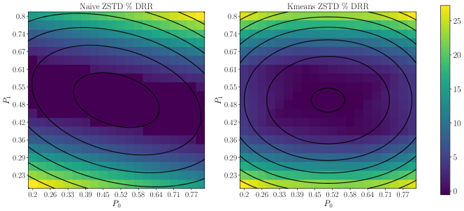
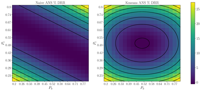
Figure 1: Comparing data reduction rate of naive coding and latent-based coding for synthetically generated data. Top: ZSTD base compressor. Bottom: ANS base compressor. Contour lines correspond to the compression rate predicted by the theorems of Section 5 (coinciding with optimal rate for latent-based encoders).

In order to better understand the limitations of classical approaches, and the optimality of latent-based compression, we introduce a probabilistic model for the table $\boldsymbol{X}^{m,n}\in{\mathcal{X}}^{m\times n}$. We assume the true latents $(u_{i})_{i\leq m}$, $(v_{j})_{j\leq n}$ to be independent random variables with

$${\mathbb{P}}(u_{i}=u)=q_{\mbox{\small\rm r}}(u)\,,\;\;\;\;{\mathbb{P}}(v_{i}=v)=q_{\mbox{\small\rm c}}(v)\,.$$ (4.1)

We assume that the entries $(X_{ij})_{i\leq m,j\leq n}$ are conditionally independent given ${\boldsymbol{u}}^{m}=(u_{i})_{i\leq m}$ ${\boldsymbol{v}}^{n}=(v_{j})_{j\leq n}$, with

$${\mathbb{P}}\big{(}X_{ij}=x\big{|}{\boldsymbol{u}}^{m},{\boldsymbol{v}}^{n}\big{)}=Q(x|u_{i},v_{j})\,.$$ (4.2)

The distributions $q_{\mbox{\small\rm r}},q_{\mbox{\small\rm c}}$, and conditional distribution $Q$ are parameters of the model (a total of $2(|{\cal L}|-1)+|{\cal L}|^{2}(|{\mathcal{X}}|-1)$ real parameters). We will write $(\boldsymbol{X}^{m,n},{\boldsymbol{u}}^{m},{\boldsymbol{v}}^{n})\sim{\mathcal{T}}(Q,q_{\mbox{\small\rm r}},q_{\mbox{\small\rm c}};m,n)$ to indicate that the triple $(\boldsymbol{X}^{m,n},{\boldsymbol{u}}^{m},{\boldsymbol{v}}^{n})$ is distributed according to the model.

Remark 4.1.

Some of our statements will be non-asymptotic, in which case $m$, $n$, ${\mathcal{X}}$, ${\cal L}$, $Q$, $q_{\mbox{\small\rm r}}$, $q_{\mbox{\small\rm c}}$ are fixed. Others will be of asymptotic. In the latter case, we have in mind a sequence of problems indexed by $n$. In principle, we could write $m_{n}$, ${\mathcal{X}}_{n}$, ${\cal L}_{n}$, $Q_{n}$, $q_{\mbox{\small\rm r},n}$, $q_{\mbox{\small\rm c},n}$ to emphasize the fact that these quantities depend on $n$. However, we will typically omit these subscripts.

Example 4.2 (Symmetric Binary Model).

As a toy example, we will use the following Symmetric Binary Model (SBM) which parallels the symmetric stochastic block model for community detection [HLL83]. We take ${\cal L}=[k]:=\{1,\dots,k\}$, ${\mathcal{X}}=\{0,1\}$, $q_{\mbox{\small\rm r}}=q_{\mbox{\small\rm c}}={\sf Unif}([k])$ (the uniform distribution over $[k]$) and

$$Q(1|u,v)=\begin{cases}p_{1}&\mbox{ if $u=v$,}\\ p_{0}&\mbox{ if $u\neq v$.}\\ \end{cases}$$ (4.3)

We will write $(\boldsymbol{X}^{m,n},{\boldsymbol{u}}^{m},{\boldsymbol{v}}^{n})\sim{\mathcal{T}}_{\mbox{\tiny\rm SBM}}(p_{0},p_{1},k;m,n)$ when this distribution is used.

Figure 1 reports the results of simulations within this model, for ZSTD and ANS base compressors. In this case $m=n=1000$, $k=3$, and we average DRR values over $4$ realizations. Appendix B reports additional simulations under the same model for $k\in\{5,7\}$: the results are very similar to the ones of Figure 1. As expected, the use of latents is irrelevant along the line $p_{1}\approx p_{0}$ (in this case, the latents do not impact the distribution of $X_{ij}$). However, it becomes important when $p_{1}$ and $p_{0}$ are significantly different.

The figures also report contour lines of the theoretical predictions for the asymptotic DRR of various compression algorithms (cf. Example 5.4). The agreement is excellent.

5 Theoretical analysis

In this section we present our theoretical results on compression rates under the model ${\mathcal{T}}(Q,q_{\mbox{\small\rm r}},q_{\mbox{\small\rm c}},k;m,n)$ introduced above. We first characterize the optimal compression rate in Section 5.1, then prove that standard compression methods fail to attain this goal in Section 5.2, and finally show that latent-based compression does in Section 5.3. Proofs are deferred to Appendices D, E, F, G.

Throughout, we denote by $(X,U,V)$ a triple with joint distribution ${\mathbb{P}}(X=x,U=u,V=v)=Q(x|u,v)q_{\mbox{\small\rm r}}(u)q_{\mbox{\small\rm c}}(v)$ (this is the same as the joint distribution of $(X_{ij},u_{i},v_{j})$ for fixed $i,j$).

5.1 Ideal compression

Our first lemma provides upper and lower bounds on the entropy per symbol $H(\boldsymbol{X}^{m,n})/mn$.

Lemma 5.1.

Defining $H_{m,n}^{+}(X|U,V):=H(X|U,V)+\frac{1}{n}H(U)+\frac{1}{m}H(V)$, we have

$$H(X|U,V)\leq\frac{1}{mn}H(\boldsymbol{X}^{m,n})\leq H^{+}_{m,n}(X|U,V)\,.$$ (5.1)

Further, for any estimators ${\boldsymbol{\widehat{u}}}:{\mathcal{X}}^{m\times n}\to{\cal L}^{m}$, ${\boldsymbol{\widehat{v}}}:{\mathcal{X}}^{m\times n}\to{\cal L}^{n}$, let $\,{\sf Err}_{U}:=\min_{\pi\in{\mathfrak{S}}_{{\cal L}}}\sum_{i=1}^{m}{\boldsymbol{1}}_{\hat{u}_{i}\neq\pi(u_{i})}/m$, $\,{\sf Err}_{V}:=\min_{\pi\in{\mathfrak{S}}_{{\cal L}}}\sum_{i=1}^{n}{\boldsymbol{1}}_{\hat{v}_{i}\neq\pi(v_{i})}/n$ ($\min$ over permutations of ${\cal L}$), letting ${\varepsilon}_{U}:={\mathbb{E}}\,{\sf Err}_{U}$, ${\varepsilon}_{V}:={\mathbb{E}}\,{\sf Err}_{V}$, we have

$$H^{+}_{m,n}(X|U,V)-\delta_{m,n}\leq\frac{1}{mn}H(\boldsymbol{X}^{m,n})\leq H^{+}_{m,n}(X|U,V)\,.$$ (5.2)

where $\delta_{m,n}:=\delta({\varepsilon}_{U})/n+\delta({\varepsilon}_{V})/m$ and $\delta({\varepsilon}):={\sf h}({\varepsilon})+{\varepsilon}\log(|{\cal L}|-1)$.

Corollary 5.2.

There exists a lossless compressor $\phi$ whose rate (cf.Eq. (3.2)) is

$${\mathbb{E}}\,{\sf R}_{\phi}(\boldsymbol{X}^{m,n})\leq\frac{1}{\log_{2}|{\mathcal{X}}|}\Big{\{}H^{+}_{m,n}(X|U,V)+\frac{1}{mn}\Big{\}}\,.$$ (5.3)

Further, for any lossless compressor $\phi$, ${\mathbb{E}}\,{\sf R}_{\phi}(\boldsymbol{X}^{m,n})\geq H^{+}_{m,n}(X|U,V)-\delta_{m,n}-2\log_{2}(mn)/mn$.

Remark 5.1.

The simpler bound (5.1) implies that the entropy per entry is $H(X|U,V)+O(1/(m\wedge n))$. The operational interpretation of this result is that we should be able to achieve the same compression rate per symbol as if the latents were given to us.

The additional terms $\frac{1}{n}H(U)+\frac{1}{m}H(V)$ in Eq. (5.2) account for the additional memory required for the latents. The lower bound in Eq. (5.2) implies that, if the latents can be accurately estimated from the data $\boldsymbol{X}^{m,n}$ (that is if ${\varepsilon}_{U}$, ${\varepsilon}_{V}$ are small), then this overhead is essentially unavoidable.

The nearly ideal compression rate in Eq. (5.3) can be achieved by Huffmann or arithmetic coding, and requires knowledge of the probability distribution of $\boldsymbol{X}^{m,n}$. Under the these schemes, the length of the codeword associated to $\boldsymbol{X}^{m,n}$ is within constant number of bits from $-\log_{2}{\rm P}(\boldsymbol{X}^{m,n})$, where ${\rm P}(\boldsymbol{X}_{0}):={\mathbb{P}}(\boldsymbol{X}^{m,n}=\boldsymbol{X}_{0})$ is the probability mass function of the random table $\boldsymbol{X}^{m,n}$ [CT06, Sal04]. The next lemma implies that the length concentrates tightly around the entropy.

Lemma 5.3 (Asymptotic Equipartition Property).

For $\boldsymbol{X}_{0}\in{\mathcal{X}}^{m\times n}$, let ${\rm P}(\boldsymbol{X}_{0})={\rm P}_{Q,q_{\mbox{\small\rm r}},q_{\mbox{\small\rm c}};m,n}(\boldsymbol{X}_{0})$ the probability of $\boldsymbol{X}^{m,n}=\boldsymbol{X}_{0}$ under model $\boldsymbol{X}^{m,n}\sim{\mathcal{T}}(Q,q_{\mbox{\small\rm r}},q_{\mbox{\small\rm c}};m,n)$. Assume there exists a constant $c>0$ such that $\min_{x\in{\mathcal{X}}}\min_{u,v\in{\cal L}}Q(x|u,v)\geq c$. Then there exists a constant $C$ (depending on $c$) such that the following happens.

For $\boldsymbol{X}^{m,n}\sim{\mathcal{T}}(Q,q_{\mbox{\small\rm r}},q_{\mbox{\small\rm c}};m,n)$ and any $t\geq 0$ with probability at least $1-2\,e^{-t}$:

$$\big{|}-\log{\rm P}(\boldsymbol{X}^{m,n})-H(\boldsymbol{X}^{m,n})\big{|}\leq C\sqrt{mn(m+n)}\,t\,.$$ (5.4)

For the sake of simplicity, in the last statement we assume a uniform lower bound on $Q(x|u,v)$. While such a lower bound holds without loss of generality when $Q$ is independent of $m,n$ (symbols with zero probability can be dropped), it might not hold in the $n$-dependent case. Appendix D gives a more general statement.

5.2 Failure of classical compression schemes

We analyze two types of codes: finite-state encoders and Lempel-Ziv codes. Both operate on the serialized data $\boldsymbol{X}^{N}={\sf vec}(\boldsymbol{X}^{m,n})$, $N=mn$, obtained by scanning the table in row-first order (obviously column-first yields symmetric results).

5.2.1 Finite state encoders

A finite state (FS) encoder takes the form of a triple $(\Sigma,f,g)$ with $\Sigma$ a finite set of cardinality $M=|\Sigma|$ and $f:{\mathcal{X}}\times\Sigma\to\{0,1\}^{*}$, $g:{\mathcal{X}}\times\Sigma\to\Sigma$.

We assume that $\Sigma$ contains a special ‘initialization’ symbol $s_{\mbox{\tiny\rm init}}$. Starting from state $s_{0}=s_{\mbox{\tiny\rm init}}$, the encoder scans the input $\boldsymbol{X}^{N}$ sequentially. Assume after the first $\ell$ input symbols it is in state $s_{\ell}$, and produced encoding ${\boldsymbol{z}}_{1}^{k(\ell)}$. Given input symbol $X_{\ell+1}$, it appends $f(X_{\ell+1},s_{\ell})$ to the codeword, and updates its state to $s_{\ell+1}=g(X_{\ell+1},s_{\ell})$.

With an abuse of notation, denote by $f_{\ell}(\boldsymbol{X}^{\ell},s_{\mbox{\tiny\rm init}})\in\{0,1\}^{*}$ the binary sequence obtained by applying the finite state encoder to $\boldsymbol{X}^{\ell}=(X_{1},\dots,X_{\ell})$ We say that the FS encoder is information lossless if for any $\ell\in{\mathbb{N}}$, $\boldsymbol{X}^{\ell}\mapsto f_{\ell}(\boldsymbol{X}^{\ell},s_{\mbox{\tiny\rm init}})$ is injective.

Theorem 5.4.

Let $\boldsymbol{X}=\boldsymbol{X}^{m,n}\sim{\mathcal{T}}(Q,q_{\mbox{\small\rm r}},q_{\mbox{\small\rm c}};m,n)$ and $\phi:=(\Sigma,f,g)$ be an information lossless finite state encoder. Define the corresponding compression rate ${\sf R}_{\phi}(\boldsymbol{X})$, as per Eq. (3.2). Assuming $m>10$, $|\Sigma|\geq|{\mathcal{X}}|$, and $\log_{2}|\Sigma|\leq n\log_{2}|{\mathcal{X}}|/9$,

$${\mathbb{E}}\,{\sf R}_{\phi}(\boldsymbol{X}) \geq\frac{H(X|U)}{\log_{2}|{\mathcal{X}}|}-10\sqrt{\frac{\log|\Sigma|}{n\log|{\mathcal{X}}|}}\cdot\log(n\log|\Sigma|)\,.$$ (5.5)

Remark 5.2.

The leading term of the above lower bound is $H(X|U)/\log_{2}|{\mathcal{X}}|$. Since conditioning reduces entropy, this is strictly larger than the ideal rate which is roughly $H(X|U,V)/\log_{2}|{\mathcal{X}}|$, cf. Eq. (5.3).

The next term is negligible provided $\log|\Sigma|\ll n\log|{\mathcal{X}}|$. This condition is easy to interpret: it amounts to say that the finite state machine does not have enough states to memorize a row of the table $\boldsymbol{X}^{m,n}$.

5.2.2 Lempel-Ziv

The pseudocode of the Lempel-Ziv algorithm that we will analyze is given in Appendix F.

In words, after the first $k$ characters of the input have been parsed, the encoder finds the longest string $\boldsymbol{X}_{k}^{k+\ell-1}$ which appears in the past. It then encodes a pointer to the position of the earlier appearance of the string $T_{k}$, and its length $L_{k}$. If a simbol $X_{k}$ never appeared in the past, we use a special encoding, cf. Appendix F.

We encode the pointer $T_{k}$ in plain binary using $\lceil\log_{2}(N+|{\mathcal{X}}|)\rceil$ bits (note that $T_{k}\in\{-|{\mathcal{X}}|+1,\dots,1,\dots,N\}$), and $L_{k}$ using an instantaneous prefix-free code, e.g. Elias $\delta$-coding, taking $2\lfloor\log_{2}L_{k}\rfloor+1$ bits.

Assumption 5.5.

There exist a constant $c_{0}>0$ such that

$$\max_{x\in{\mathcal{X}}}\max_{u,v\in{\cal L}}Q(x|u,v)\leq 1-c_{0}\,.$$

Further $Q,q_{\mbox{\small\rm r}},co,{\mathcal{X}},{\cal L}$ are fixed and $m,n\to\infty$ with $m=n^{\alpha+o(1)}$, i.e.

$$\lim_{n\to\infty}\frac{\log m}{\log n}=\alpha\in(0,\infty)\,.$$ (5.6)

As mentioned above, we consider sequences of instances with $m,n\to\infty$. If convenient, the reader can think this sequence to be indexed by $n$, and let $m=m_{n}$ depend on $n$ such that Eq. (5.6) holds.

Theorem 5.6.

Under Assumption 5.5, the asymptotic Lempel-Ziv rate is

$$\lim_{m,n\to\infty} {\mathbb{E}}\,{\sf R}_{{\sf LZ}}(\boldsymbol{X}^{m,n})={\sf R}_{{\sf LZ}}^{\infty}:=\sum_{u\in{\cal L}}\frac{q_{\mbox{\small\rm r}}(u){\sf R}_{{\sf LZ}}^{\infty}(u)}{\log_{2}|{\mathcal{X}}|}\,,$$ (5.7)

$${\sf R}_{{\sf LZ}}^{\infty}(u) :=H(X|U=u)\wedge\Big{(}\frac{1+\alpha}{\alpha}\Big{)}H(X|U=u,V)\,.$$

Remark 5.3.

The asymptotics of the Lempel-Ziv rate is given by the minimum of two expressions, which correspond to different behaviors of the encoder. For $u\in{\cal L}$, define $\alpha_{*}(u):=H(X|U=u,V)/(H(X|U=u)-H(X|U=u,V))$ (with $\alpha_{*}(u)=\infty$ if $H(X|U=u)=H(X|U=u,V)$). Then:

If $\alpha<\alpha_{*}(u)$, then we are a ‘skinny table’ regime. The algorithm mostly deduplicates segments in rows with latent $u$ by using strings in different rows but aligned in the same columns. If $\alpha>\alpha_{*}(u)$, then we are a ‘fat table’ regime. The algorithm mostly deduplicates segments on rows with latent $u$ by using rows and columns that are not the same as the current segment.

Example 5.4 (Symmetric Binary Model, dense regime).

Under the Symmetric Binary Model ${\mathcal{T}}_{\mbox{\tiny\rm SBM}}(p_{0},p_{1},k;m,n)$ of Example 4.2, we can compute the optimal compression rate of Corollary 5.2, the finite state compression rate of Theorem 5.4, the Lempel-Ziv rate of Theorem 5.6.

If $p_{0}$, $p_{1}$ are of order one, and $m=n^{\alpha+o_{n}(1)}$ as $m,n\to\infty$, letting $\overline{p}:=((k-1)/k)p_{0}+(1/k)\,p_{1}$, $\overline{{\sf h}}(p_{0},p_{1}):=((k-1)/k){\sf h}(p_{0})+(1/k)\,{\sf h}(p_{1})$, we obtain:

$${\mathbb{E}}\,{\sf R}_{\mbox{\tiny\rm opt}}(\boldsymbol{X}) =\Big{(}1-\frac{1}{k}\Big{)}\,{\sf h}(p_{0})+\frac{1}{k}\,{\sf h}(p_{1})+o_{n}(1)\,,$$

$${\mathbb{E}}\,{\sf R}_{\mbox{\tiny\rm fin. st.}}(\boldsymbol{X}) \geq{\sf h}(\overline{p})+o_{n}(1)\,,$$

$${\mathbb{E}}\,{\sf R}_{{\sf LZ}}(\boldsymbol{X}) ={\sf h}(\overline{p})\wedge\Big{(}\frac{1+\alpha}{\alpha}\Big{)}\overline{{\sf h}}(p_{0},p_{1})+o_{n}(1)\,.$$

These theoretical predictions are used to trace the contour lines in Figure 1. (ANS coding is implemented as a finite state code here.)

5.3 Practical latent-based compression

Achieving the ideal rate of Corollary 5.2 via arithmetic or Huffmann coding requires to compute the probability ${\rm P}(\boldsymbol{X}^{m,n})$, which is intractable. We will next show that we can achieve a compression rate that is close to the ideal rate via latents estimation.

We begin by considering general latents estimators ${\boldsymbol{\widehat{u}}}:{\mathcal{X}}^{m\times n}\to{\cal L}^{m}$, ${\boldsymbol{\widehat{v}}}:{\mathcal{X}}^{m\times n}\to{\cal L}^{n}$. We measure their accuracy by the error (cf. Lemma 5.1)

$$\,{\sf Err}_{U}(\boldsymbol{X};{\boldsymbol{\widehat{u}}}):=\frac{1}{m}\min_{\pi\in{\mathfrak{S}}_{{\cal L}}}\sum_{i=1}^{m}\Big{\{}{\boldsymbol{1}}_{\hat{u}_{i}(\boldsymbol{X})\neq\pi(u_{i})}\Big{\}}$$

and the analogous $\,{\sf Err}_{V}(\boldsymbol{X};{\boldsymbol{\widehat{v}}})$. Here the minimization is over the set ${\mathfrak{S}}_{{\cal L}}$ of permutations of the latents alphabet ${\cal L}$.

We can use any estimators ${\boldsymbol{\widehat{u}}}$, ${\boldsymbol{\widehat{v}}}$ to reorder rows and columns and compress the table $\boldsymbol{X}^{m,n}$ according to the algorithm described in the introduction. We denote by ${\sf R}_{{\mbox{\tiny\rm lat}}}(\boldsymbol{X})$ the compression rate achieved by such a procedure.

Our first result implies that, if the latent estimators are consistent (namely, they recover the true latents with high probability, up to permutations), then the resulting rate is close to the ideal one.

Lemma 5.7.

Assume data distributed according to model $\boldsymbol{X}^{m,n}\sim{\mathcal{T}}(Q,q_{\mbox{\small\rm r}},q_{\mbox{\small\rm c}};m,n)$, with $m,n\geq\log_{2}|{\cal L}|$. Further assume there exists $c_{0}>0$ such that $q_{\mbox{\small\rm r}}(u),q_{\mbox{\small\rm c}}(v)\geq c_{0}$ for all $u,v\in{\cal L}$. Let ${\sf R}_{{\mbox{\tiny\rm lat}}}(\boldsymbol{X})$ be the rate achieved by the latent-based scheme with latents estimators ${\boldsymbol{\widehat{u}}}$, ${\boldsymbol{\widehat{v}}}$, and base encoders ${\sf Z}_{{\mathcal{X}}}={\sf Z}_{{\cal L}}={\sf Z}$. Then

$${\mathbb{E}}\,{\sf R}_{{\mbox{\tiny\rm lat}}} (\boldsymbol{X})\leq\frac{H(\boldsymbol{X}^{m,n})}{mn\log_{2}|{\mathcal{X}}|}+2P_{\mbox{\tiny\rm err}}(m,n)+\frac{4\log(mn)}{mn}$$

$$+|{\cal L}|^{2}\Delta_{{\sf Z}}(c\cdot mn;\mathscrsfs{Q})+2\Delta_{{\sf Z}}(m\wedge n;\{q_{\mbox{\small\rm r}},q_{\mbox{\small\rm c}}\})\,.$$ (5.8)

Here $P_{\mbox{\tiny\rm err}}(m,n):={\mathbb{P}}(\,{\sf Err}_{U}(\boldsymbol{X}^{m,n};{\boldsymbol{\widehat{u}}})>0)+{\mathbb{P}}(\,{\sf Err}_{V}(\boldsymbol{X}^{m,n};{\boldsymbol{\widehat{v}}})>0)$, $\Delta_{{\sf Z}}(N;\mathscrsfs{P}_{*})$ is the worst-case redundancy of encoder ${\sf Z}$ over i.i.d. sources with distributions in $\mathscrsfs{P}_{*}$ (see comments below), $\mathscrsfs{Q}:=\{Q(\,\cdot\,|u,v)\}_{u,v\in{\cal L}}$.

The redundancies of Lempel-Ziv, frequency-based arithmetic coding and ANS coding can be upper bounded as (in the last bound $Q,q_{\mbox{\small\rm r}},q_{\mbox{\small\rm c}}$ need to be be independent of $N$)

$$\Delta_{{\sf LZ}}(N;\mathscrsfs{P}_{*}) \leq 40c_{*}(\mathscrsfs{P}_{*})\Big{(}\frac{\log\log N}{\log N}\Big{)}^{1/2}\,,$$ (5.9)

$$\Delta_{{\sf AC}}(N;\mathscrsfs{P}_{*}) \leq\frac{2|{\mathcal{X}}|}{\log|{\mathcal{X}}|}\cdot\frac{\log N}{N}\,,$$ (5.10)

$$\Delta_{{\sf ANS}}(N;\mathscrsfs{P}_{*}) \leq\frac{2|{\mathcal{X}}|\log N+C_{|{\mathcal{X}}|}}{N}\,.$$ (5.11)

Here Eq. (5.9) holds for $N\geq\exp\{\sup_{q\in\mathscrsfs{P}_{*}}(4\log(2/H(q)))^{2}\}$, and $c_{*}(\mathscrsfs{P}_{*}):=\sup_{q\in\mathscrsfs{P}_{*}}\sum_{x\in{\mathcal{X}}}(\log q(x))^{2}/|{\mathcal{X}}|$.

The proof of this lemma is given in Appendix G.1. The main content of the lemma is in the general bound (5.8) which is proven in Appendix G.1.1.

Remark 5.5.

We define the worst case redundancy $\Delta_{{\sf Z}}(N_{0};\mathscrsfs{P}_{*}):=\max_{N\geq N_{0}}\widehat{\Delta}_{{\sf Z}}(N;\mathscrsfs{P}_{*})$, where

$$\widehat{\Delta}_{{\sf Z}}(N;\mathscrsfs{P}_{*}):=\max_{q\in\mathscrsfs{P}_{*}}\frac{{\mathbb{E}}_{q}{\sf len}({\sf Z}(\boldsymbol{Y}^{N}))-H(\boldsymbol{Y}^{N})}{N\log_{2}k}\,,$$ (5.12)

where $\mathscrsfs{P}_{*}\subseteq\mathscrsfs{P}([k]):=\{(p_{i})_{i\leq k}\in{\mathbb{R}}^{k}:p_{i}\geq 0\,\forall i\,\mbox{ and }\sum_{i\leq k}p_{i}=1\}$ is a set of probability distributions over $[k]$ and $\boldsymbol{Y}^{N}$ is a vector with i.i.d. entries $Y_{i}\sim q$.

While Eqs. (5.9)—(5.11) are closely related to well known facts, there are nevertheless differences with respect to statements in the literature. We address them in Section G.1.2. Perhaps the most noteworthy difference is in the bound (5.9) for the LZ algorithm. Existing results, e.g. Theorem 2 in [Sav98], assume a single, $N$-independent, distribution $q$ and are asymptotic in nature. Equation (5.9) is a non-asymptotic statement and applies to a collection of distributions $\mathscrsfs{P}_{*}$ that could depend on $N$.

Lemma 5.7 can be used in conjunction with any latent estimation algorithm, as we next demonstrate by considering the spectral algorithm of Section 2.2. Recall that the algorithm makes use of a map $\psi:{\mathcal{X}}\to{\mathbb{R}}$. For $(X,U,V)\sim Q(\,\cdot\,|\,\cdot\,,\,\cdot\,)q_{\mbox{\small\rm r}}(\,\cdot\,)q_{\mbox{\small\rm c}}(\,\cdot\,)$, we define $\overline{\psi}(u,v):={\mathbb{E}}[\psi(X)|U=u,V=v]$, ${\boldsymbol{\Psi}}:=\big{(}\overline{\psi}(u,v)\big{)}_{u,v\in{\cal L}}$ and the parameters:

$$\mu_{n}:=\sigma_{\min}({\boldsymbol{\Psi}})\,,\;\;\nu_{n}:=\max_{u,v\in{\cal L}}|\overline{\psi}(u,v)|\,,$$ (5.13)

$$\sigma_{n}^{2}:=\max_{u,v\in{\cal L}}{\rm Var}\big{(}\psi(X)|U=u,V=v\big{)}\,.$$ (5.14)

We further will assume, without loss of generality $\max_{x\in{\mathcal{X}}}|\psi(x)|\leq 1$.

Finally, we need to formally specify the version of the KMeans primitive in the spectral clustering algorithm. In fact, we establish correctness for a simpler thresholding procedure. Considering to be definite the row latents, and for a given threshold $\theta>0$, we construct a graph $G_{\theta}=([m],E_{\theta})$ by letting (for distinct $i,j\in[m]$)

$$\frac{\|{\boldsymbol{a}}_{i}-{\boldsymbol{a}}_{j}\|_{2}}{(\|{\boldsymbol{a}}_{i}\|_{2}+\|{\boldsymbol{a}}_{j}\|_{2})/2}\leq\theta\;\;\Leftrightarrow\;\;(i,j)\in E_{\theta}\,.$$ (5.15)

The algorithm then output the connected components of $G_{\theta}$.

Theorem 5.8.

Assume data $\boldsymbol{X}^{m,n}\sim{\mathcal{T}}(Q,q_{\mbox{\small\rm r}},q_{\mbox{\small\rm c}};m,n)$, with $m,n\geq\log_{2}|{\cal L}|$ and $\min_{u\in{\cal L}}(q_{\mbox{\small\rm r}}(u)\wedge q_{\mbox{\small\rm c}}(u))\geq c_{0}$ for a constant $c_{0}>0$. Let ${\sf R}_{{\mbox{\tiny\rm lat}}}(\boldsymbol{X})$ be the rate achieved by the latent-based scheme with spectral latents estimators ${\boldsymbol{\widehat{u}}}$, ${\boldsymbol{\widehat{v}}}$, base compressors ${\sf Z}_{{\mathcal{X}}}={\sf Z}_{{\cal L}}={\sf Z}$, and thresholding algorithm as described above. Then, assuming $\sigma_{n}\geq c\sqrt{(\log n)/n}$, $\nu_{n}/\sigma_{n}\leq c\sqrt{\log n}$ $\mu_{n}\geq C(\sigma_{n}\sqrt{(\log n)/m}\vee(\log n)/\sqrt{mn})$, $\theta\leq\sqrt{c_{0}}/100$, we have

$${\mathbb{E}}\,{\sf R}_{{\mbox{\tiny\rm lat}}} (\boldsymbol{X})\leq\frac{H(\boldsymbol{X}^{m,n})}{mn\log_{2}|{\mathcal{X}}|}+\frac{10\log(mn)}{mn}$$

$$+|{\cal L}|^{2}\Delta_{{\sf Z}}(c\cdot mn;\mathscrsfs{Q})+2\Delta_{{\sf Z}}(m\wedge n;\{q_{\mbox{\small\rm r}},q_{\mbox{\small\rm c}}\})\,.$$

We focus on the simpler thresholding algorithm of Eq. (5.15) instead of KMeans in order to avoid technical complications that are not the main focus of this paper. We expect it to be relatively easy to generalize this result, e.g. using the results of [MRS20] for KMeans++.

Example 5.6.

Consider the Symmetric Binary Model ${\mathcal{T}}_{\mbox{\tiny\rm SBM}}(p_{0},p_{1},k;m,n)$ of Example 4.2, with $p_{0}=p_{0,n}$, $p_{1}=p_{1,n}$ potentially dependent on $n$. Since in this case ${\mathcal{X}}=\{0,1\}$ the choice of the map $\psi$ has little impact and we set $\psi(x)=x$. We assume, to simplify formulas, $|p_{1,n}-p_{0,n}|\leq kp_{0,n}$, $p_{1,n}\vee p_{0,n}\leq 9/10$. It is easy to compute $\mu_{n}=|p_{1,n}-p_{0,n}|$, $\nu_{n}=p_{0,n}\vee p_{1,n}$, $\sigma^{2}_{n}\asymp p_{1,n}\vee p_{0,n}$:

Theorem 5.8 implies nearly optimal compression rate under the following conditions on the model parameters:

$$p_{1,n}\vee p_{0,n}\gtrsim\sqrt{\frac{\log n}{n}}\,,\;\;\;\;\;|p_{1,n}-p_{0,n}|\gtrsim\frac{\log n}{\sqrt{mn}}\,,$$

$$\frac{|p_{1,n}-p_{0,n}|}{p_{1,n}\vee p_{0,n}}\gtrsim\sqrt{\frac{\log n}{n}}\,.$$

Here $\gtrsim$ hides factors depending on $k,c_{0}$. The last of these condition amounts to requiring that the signal-to-noise ratio is large enough to consistently reconstruct the latents. In the special case of square symmetric matrices ($m=n$), sharp constants in these bounds can be derived from [Abb17].

6 Discussion and extensions

We proved that classical lossless compression schemes, that serialize the data and then apply a finite state encoder or a Lempel-Ziv encoder to the resulting sequence are sub-optimal when applied to tabular data. Namely, we introduced a simple model for tabular data, and made the following novel contributions:

1. We characterized the optimal compression rate under this model.

2. We rigorously quantified the gap in compression rate suffered by classical compressors.

3. We showed that a compression scheme that estimates the latents performs well in practice and provably achieves optimal rate on our model.

The present work naturally suggests several extensions.

Faster spectral clustering via randomized linear algebra. We implemented row subsampling singular value decomposition [DKM06], and observed hardly no loss in DRR by using $10\%$ of the rows.

Bits back coding. As mentioned several times, encoding the latents is sub-optimal, unless these can be estimated accurately in the sense of ${\mathbb{E}}\,{\sf Err}_{U}(\boldsymbol{X};{\boldsymbol{\widehat{u}}})\to 0$, ${\mathbb{E}}\,{\sf Err}_{V}(\boldsymbol{X};{\boldsymbol{\widehat{v}}})\to 0$, cf. Lemma 5.1. If this is not the case, then optimal rates can be achieved using bits-back coding.

Continuous latents. Of course, using discrete latents is somewhat un-natural, and it would be interesting to consider continuous ones, in which case bits-back coding is required.

Appendix A Details on the empirical evaluation

A.1 Datasets

We used the following datasets:

• Taxicab. A table with $m=62,495$ rows, $n_{0}=20$ columns comprising data for taxi rides in NYC during January 2022 [NYC22]. After preprocessing this table has $n=18$ columns. For the LZ (ZSTD) compressor we used $|{\cal L}_{r}|=9$ row latents and $15$ column latents, for the ANS compressor we used $|{\cal L}_{r}|=5$ row latents and 14 column latents.

• Network. Four social networks from SNAP Datasets, representing either friends as undirected edges for Facebook or directed following relationships on Google Plus [LK14]. We regard these as four distinct tables with $0-1$ entries, with dimensions, respectively $m=n\in\{333,747,786,1187\}$. For each table we used $5$ row latents and $5$ column latents.

• Card transactions. A table of simulated credit card transactions containing information like card ID, merchant city, zip, etc. This table has $m=24,386,900$ rows and $n_{0}=15$ columns and was generated as described in [Alt19] and downloaded from [IBM22]. After preprocessing the table has $n=12$ columns. For this table we used $3$ row latents and $n$ column latents.

• Business price index. A table of the values of the consumer price index of various goods in New Zealand between 1996 and 2022. This is a table with $m=72,750$ rows and $n_{0}=12$ columns from the Business price indexes: March 2022 quarter - CSV file from [sta22]. After preprocessing this table has $n=10$ columns. Due to the highly correlated nature of consecutive rows, we first shuffle them before compressing. For the LZ method we used $6$ row latents and $7$ column latents, for the ANS method we used $2$ row latents and $6$ column latents.

• Forest. A table from the UCI data repository comprising $m=581,011$ cartographic measurements with $n_{0}=55$ attributes, to predict forest cover type based on information gathered from US Geological Survey [DG17]. It contains binary qualitative variables, and some continuous values like elevation and slope. After preprocessing this data has $n=55$ columns. For the LZ method we used $6$ row latents and $17$ column latents, for the ANS method we used $6$ row latents and 17 column latents.

• US Census. Another table from the UCI Machine Learning Repository [DG17] with $m=2,458,285$ and $n_{0}=68$ categorical attributes related to demographic information, income, and occupation information. After preprocessing this data has $n=68$ columns. For this data we used $9$ row latents and $n$ column latents.

• Jokes. A table containing ratings of a series of jokes by 24,983 users collected between April 1999 and May 2003 [GRGP01, GRGP]. These ratings are real numbers on a scale from $-10$ to $10$, and a value of 99 is given to jokes that were not rated. There are $m=23,983$ rows and $n_{0}=101$. The first column identifies how many jokes were rated by a user, and the rest of the columns contain the ratings. After preprocessing this data has $n=101$ columns, all quantized. For the LZ method we used $2$ row latents and $n$ column latents, for the ANS method we used $8$ row latents and $8$ column latents.

A.2 Preprocessing

We preprocessed different columns as follows:

• If a column comprises $K\leq 256$ unique values, then we map the values to $\{0,\dots,K-1\}$.

• If a column is numerical and comprises more than $256$ unique values, we calculate the quartiles for the data and map each entry to its quartile membership (0 for the lowest quartile, 1 for the next largest, 2 for the next and 3 for the largest).

• If a column does not meet either of the above criteria, we discard it.

Finally, in some experiments we randomly permuted before compression. The rationale is that some of the above datasets have rows already ordered in a way that makes nearby rows highly correlated. In these cases, row reordering is –obviously– of limited use.

Appendix B Further simulations

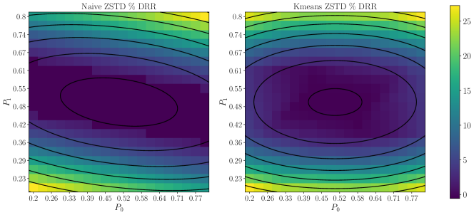
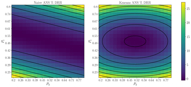
Figure 2: Comparing data reduction rate of naive coding and latent-based coding for data from SBM with $k=5$ latents. Top row: ZSTD base compressor. Bottom row: ANDS base compressor. Contour lines correspond to the theoretical predictions for various compression algorithms (cf. Example 5.4).

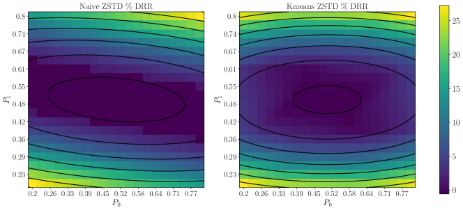
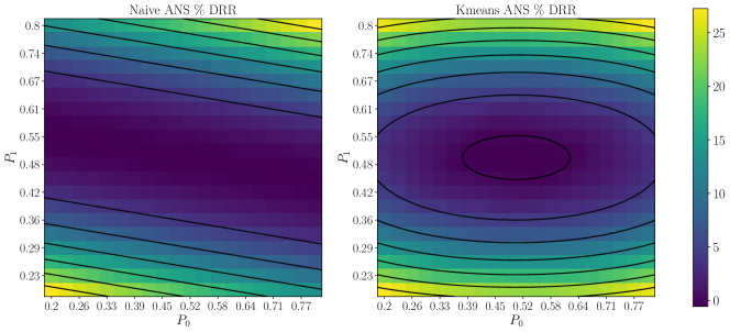
Figure 3: Same as Figure 2 with $k=7$.

Figures 2 and 3 report empirical DRR values for ZSTD and ANS coding, for data generated according to the symmetric model ${\mathcal{T}}_{\mbox{\tiny\rm SBM}}(p_{0},p_{1},k;m,n)$ of Section 4. We use $m=n=1000$ as before, but now $k\in\{5,7\}$. Results confirm the conclusions of Section 4.

Appendix C A basic fact

Lemma C.1.

Let ${\mathcal{A}}$ be a finite set and $F:{\mathcal{A}}\to\{0,1\}^{*}$ be an injective map. Then, for any probability distribution $p$ over ${\mathcal{A}}$,

$$\sum_{a\in{\mathcal{A}}}p(a){\sf len}(F(a))\geq H(p)-\log_{2}\log_{2}(|{\mathcal{A}}|+2)\,.$$ (C.1)

Proof.

Assume without loss of generality that ${\mathcal{A}}=\{1,\dots,M\}$, with $|{\mathcal{A}}|=K$, and that the elements of ${\mathcal{A}}$ have all non-vanishing probability and are ordered by decreasing probability $p_{1}\geq p_{2}\geq\cdots\geq p_{K}>0$. Let $N_{\ell}:=2+4+\dots+2^{\ell}=2{\ell+1}-2$. Then the expected length is minimized any map $F$ such that ${\sf len}(F(a))=\ell$ for $N_{\ell-1}\leq a\leq N_{\ell}$ with the maximum length $\ell_{K}$ being defined by $N_{\ell_{K}-1}<K\leq N_{\ell_{K}}$. For $A\sim p$, $L:={\sf len}(F(A))$, we have

$$H(p) :=H(A)\stackrel{{\scriptstyle(a)}}{{\leq}}H(L)+H(A|L)$$

$$\leq\log_{2}\ell_{K}+\sum_{\ell=1}^{\ell_{K}}{\mathbb{P}}(L=\ell)H(A|L=\ell)$$

$$\stackrel{{\scriptstyle(b)}}{{\leq}}\log_{2}\ell_{K}+\sum_{\ell=1}^{\ell_{M}}{\mathbb{P}}(L=\ell)\,\ell$$

$$\leq\log_{2}\log_{2}(K+2)+\sum_{a\in{\mathcal{A}}}p(a){\sf len}(F(a))\,,$$

where $(a)$ is the chain rule of entropy and $(b)$ follows because by injectivity, given ${\sf len}(F(A))=\ell$, $A$ can take at most $2^{\ell}$ values. ∎

Appendix D Proofs of results on ideal compression

D.1 Proof of Lemma 5.1

We begin by claiming that

$$\frac{1}{mn}H(\boldsymbol{X}^{m,n})=H(X|U,V)+\frac{1}{mn}I(\boldsymbol{X}^{m,n};{\boldsymbol{U}}^{m},{\boldsymbol{V}}^{n})\,.$$ (D.1)

Indeed, by the definition of mutual information, we have $H(\boldsymbol{X}_{m,n})=H(\boldsymbol{X}_{m,n}|{\boldsymbol{U}}_{m},{\boldsymbol{V}}_{n})+I(\boldsymbol{X}_{m,n};{\boldsymbol{U}}_{m},{\boldsymbol{V}}_{n})$. Equation (D.1) follows by noting that

$$H(\boldsymbol{X}^{m,n}|{\boldsymbol{U}}^{m},{\boldsymbol{V}}^{n}) =\sum_{{\boldsymbol{u}}\in{\cal L}^{m}}\sum_{{\boldsymbol{v}}\in{\cal L}^{n}}{\mathbb{P}}({\boldsymbol{U}}^{m}={\boldsymbol{u}},{\boldsymbol{V}}^{n}={\boldsymbol{v}})\,H(\boldsymbol{X}^{m,n}|{\boldsymbol{U}}^{m}={\boldsymbol{u}},{\boldsymbol{V}}^{n}={\boldsymbol{v}})$$

$$\stackrel{{\scriptstyle(a)}}{{=}}\sum_{i=1}^{m}\sum_{j=1}^{n}\sum_{{\boldsymbol{u}}\in{\cal L}^{m}}\sum_{{\boldsymbol{v}}\in{\cal L}^{n}}{\mathbb{P}}({\boldsymbol{U}}^{m}={\boldsymbol{u}},{\boldsymbol{V}}^{n}={\boldsymbol{v}})\,H(X_{i,j}|U_{i}=u,V_{j}=v)$$

$$=\sum_{i=1}^{m}\sum_{j=1}^{n}\,\sum_{{\boldsymbol{u}}\in{\cal L}}\sum_{{\boldsymbol{v}}\in{\cal L}}{\mathbb{P}}(U_{i}=u_{i},V_{j}=v_{j})H(X_{i,j}|U_{i}=u_{i},V_{j}=v_{j})$$

$$=\sum_{i=1}^{m}\sum_{j=1}^{n}H(X_{i,j}|U_{i},V_{j})\stackrel{{\scriptstyle(b)}}{{=}}mnH(X_{1,1}|U_{1},V_{1})\,,$$

where $(a)$ follows from the fact that the $(X_{i,j})$ are conditionally independent given ${\boldsymbol{U}}^{m}$, ${\boldsymbol{V}}^{n}$, ad since the conditional distribution of $X_{i,j}$ only depends on ${\boldsymbol{U}}^{m}$, ${\boldsymbol{V}}^{n}$ via $U_{i}$, $V_{j}$; $(b)$ holds because the triples $(X_{i,j},U_{i},V_{j})$ are identically distributed.

The lower bound in Eq. (5.1) holds because mutual information is non-negative, and the upper bound because $I(\boldsymbol{X}^{m,n};{\boldsymbol{U}}^{m},{\boldsymbol{V}}^{n})\leq H({\boldsymbol{U}}^{m},{\boldsymbol{V}}^{n})=mH(U_{1})+nH(V_{1})$.

Finally, to prove Eq. (5.2), define

$$\pi_{{\boldsymbol{U}},\boldsymbol{X}}:=\arg\min_{\pi\in{\mathfrak{S}}_{{\cal L}}}\frac{1}{m}\sum_{i=1}^{m}{\boldsymbol{1}}_{\hat{u}_{i}\neq\pi(u_{i})}\,,\;\;\;\;\pi_{{\boldsymbol{V}},\boldsymbol{X}}:=\arg\min_{\pi\in{\mathfrak{S}}_{{\cal L}}}\frac{1}{n}\sum_{i=1}^{n}{\boldsymbol{1}}_{\hat{v}_{i}\neq\pi(v_{i})}\,,$$ (D.2)

If the minimizer is not unique, one can be chosen arbitrarily. We then have holds because

$$I(\boldsymbol{X}^{m,n};{\boldsymbol{U}}^{m},{\boldsymbol{V}}^{n}) =H({\boldsymbol{U}}^{m},{\boldsymbol{V}}^{n})-H({\boldsymbol{U}}^{m},{\boldsymbol{V}}^{n}|\boldsymbol{X}^{m,n})$$

$$\geq mH(U_{1})+nH(V_{1})-H({\boldsymbol{U}}^{m}|\boldsymbol{X}^{m,n})-H({\boldsymbol{V}}^{n}|\boldsymbol{X}^{m,n})$$

$$\geq mH(U_{1})+nH(V_{1})-\big{[}H({\boldsymbol{U}}^{m}|\boldsymbol{X}^{m,n},\pi_{{\boldsymbol{U}},\boldsymbol{X}})+I({\boldsymbol{U}}^{m};\pi_{{\boldsymbol{U}},\boldsymbol{X}}|\boldsymbol{X}^{m,n})\big{]}$$ (D.3)

$$\phantom{AAAA}-\big{[}H({\boldsymbol{V}}|\boldsymbol{X}^{m,n},\pi_{{\boldsymbol{V}},\boldsymbol{X}})+I({\boldsymbol{V}}^{n};\pi_{{\boldsymbol{V}},\boldsymbol{X}}|\boldsymbol{X}^{m,n})\big{]}$$

$$\geq mH(U_{1})+nH(V_{1})-H({\boldsymbol{U}}^{m}|\boldsymbol{X}^{m,n},\pi_{{\boldsymbol{U}},\boldsymbol{X}})-H({\boldsymbol{V}}|\boldsymbol{X}^{m,n},\pi_{{\boldsymbol{V}},\boldsymbol{X}})-2|{\cal L}|\log_{2}(|{\cal L}|)\,,$$ (D.4)

where in the last inequality we used the fact that $I({\boldsymbol{U}}^{m};\pi_{{\boldsymbol{U}},\boldsymbol{X}}|\boldsymbol{X}^{m,n})\leq H(\pi_{{\boldsymbol{U}},\boldsymbol{X}})\leq\log_{2}(|{\cal L}|!)$.

Now, consider the term $H({\boldsymbol{U}}^{m}|\boldsymbol{X}^{m,n},\pi_{{\boldsymbol{U}},\boldsymbol{X}})$. Letting $\boldsymbol{Y}:=(\boldsymbol{X}^{m,n},\pi_{{\boldsymbol{U}},\boldsymbol{X}})$ the stated accuracy assumption implies that there exists an estimators ${\boldsymbol{\widehat{u}}}^{+}={\boldsymbol{\widehat{u}}}^{+}(\boldsymbol{Y})$ such that

$${\varepsilon}_{U}=\frac{1}{m}\sum_{i=1}^{m}{\varepsilon}_{U,i}\,,\;\;\;\;\;{\varepsilon}_{U,i}:={\mathbb{P}}\big{(}\hat{u}^{+}_{i}(\boldsymbol{Y})\neq U_{i}\big{)}\,.$$

By Fano’s inequality

$$H({\boldsymbol{U}}^{m}|\boldsymbol{X}^{m,n},\pi_{{\boldsymbol{U}},\boldsymbol{X}}) \leq\sum_{i=1}^{m}H(U_{i}|\boldsymbol{X}^{m,n},\pi_{{\boldsymbol{U}},\boldsymbol{X}})$$

$$\leq\sum_{i=1}^{m}\big{[}{\sf h}({\varepsilon}_{U,i})+{\varepsilon}_{U,i}\log(|{\cal L}|-1)\big{]}$$

$$\leq m\big{[}{\sf h}({\varepsilon}_{U})+{\varepsilon}_{U}\log(|{\cal L}|-1)\big{]}\,,$$

where the last step follows by Jensen’s inequality. The claim (5.2) follows by substituting this bound in Eq. (D.4) and using a similar bound for $H({\boldsymbol{V}}^{n}|\boldsymbol{X}^{m,n},\pi_{{\boldsymbol{V}},\boldsymbol{X}})$.

D.2 Proof of Lemma 5.3

We begin with a technical fact.

Lemma D.1.

Let ${\boldsymbol{\xi}}=(\xi_{ij})_{i\leq m,j\leq n}$, ${\boldsymbol{\sigma}}=(\sigma_{i})_{i\leq m}$, ${\boldsymbol{\tau}}=(\tau_{j})_{\j\leq n}$ be collections of mutually independent random variables taking values in a measurable space ${\mathcal{Z}}$. $x:{\mathcal{Z}}^{3}\to{\mathcal{Z}}$, $F:{\mathcal{Z}}^{m\times n}\to{\mathbb{R}}$. Define ${\boldsymbol{x}}({\boldsymbol{\xi}},{\boldsymbol{\sigma}},{\boldsymbol{\tau}})\in{\mathbb{R}}^{m\times n}$ via ${\boldsymbol{x}}({\boldsymbol{\xi}},{\boldsymbol{\sigma}},{\boldsymbol{\tau}})_{ij}=x(\xi_{ij},\sigma_{i},\tau_{j})$.

Given a vector of independent random variables ${\boldsymbol{z}}$, we let ${\rm Var}_{z_{i}}(f({\boldsymbol{z}})):={\mathbb{E}}_{z_{i}}[(f({\boldsymbol{z}})-{\mathbb{E}}_{z_{i}}f({\boldsymbol{z}}))^{2}]$. Define the quantities

$$B_{*} :=\max_{\begin{subarray}{c}{\boldsymbol{x}},{\boldsymbol{x}}^{\prime}\in{\mathcal{Z}}^{m\times n}\\ d({\boldsymbol{x}},{\boldsymbol{x}}^{\prime})\leq 1\end{subarray}}\big{|}F({\boldsymbol{x}})-F({\boldsymbol{x}}^{\prime\prime})\big{|}\,,$$ (D.5)

$$B_{1} :=\max_{\begin{subarray}{c}{\boldsymbol{\sigma}},{\boldsymbol{\sigma}}^{\prime}\in{\mathcal{Z}}^{m}\\ d({\boldsymbol{\sigma}},{\boldsymbol{\sigma}}^{\prime})\leq 1\end{subarray}}\max_{{\boldsymbol{\tau}}\in{\mathcal{Z}}^{n}}\big{|}{\mathbb{E}}_{{\boldsymbol{\xi}}}F({\boldsymbol{x}}({\boldsymbol{\xi}},{\boldsymbol{\sigma}},{\boldsymbol{\tau}}))-{\mathbb{E}}_{{\boldsymbol{\xi}}}F({\boldsymbol{x}}({\boldsymbol{\xi}},{\boldsymbol{\sigma}}^{\prime},{\boldsymbol{\tau}}))\big{|}\,,$$ (D.6)

$$B_{2} :=\max_{{\boldsymbol{\sigma}}\in{\mathcal{Z}}^{m}}\max_{\begin{subarray}{c}{\boldsymbol{\tau}},{\boldsymbol{\tau}}^{\prime}\in{\mathcal{Z}}^{n}\\ d({\boldsymbol{\tau}},{\boldsymbol{\tau}}^{\prime})\leq 1\end{subarray}}\big{|}{\mathbb{E}}_{{\boldsymbol{\xi}}}F({\boldsymbol{x}}({\boldsymbol{\xi}},{\boldsymbol{\sigma}},{\boldsymbol{\tau}}))-{\mathbb{E}}_{{\boldsymbol{\xi}}}F({\boldsymbol{x}}({\boldsymbol{\xi}},{\boldsymbol{\sigma}},{\boldsymbol{\tau}}^{\prime}))\big{|}\,,$$ (D.7)

$$V_{*} :=\sup_{{\boldsymbol{\xi}},{\boldsymbol{\tau}},{\boldsymbol{\sigma}}}\sum_{i\leq m,j\leq n}{\rm Var}_{\xi_{ij}}\big{\{}F({\boldsymbol{x}}({\boldsymbol{\xi}},{\boldsymbol{\sigma}},{\boldsymbol{\tau}}))\big{\}}\,,$$ (D.8)

$$V_{1} :=\sup_{{\boldsymbol{\tau}},{\boldsymbol{\sigma}}}\sum_{i\leq m}{\rm Var}_{\sigma_{i}}\big{\{}{\mathbb{E}}_{{\boldsymbol{\xi}}}F({\boldsymbol{x}}({\boldsymbol{\xi}},{\boldsymbol{\sigma}},{\boldsymbol{\tau}})\big{\}}\,,$$ (D.9)

$$V_{2} :=\sup_{{\boldsymbol{\tau}},{\boldsymbol{\sigma}}}\sum_{j\leq n}{\rm Var}_{\sigma_{j}}\big{\{}{\mathbb{E}}_{{\boldsymbol{\xi}}}F({\boldsymbol{x}}({\boldsymbol{\xi}},{\boldsymbol{\sigma}},{\boldsymbol{\tau}}))\big{\}}\,.$$ (D.10)

Then, for any $t\geq 0$, the following holds with probability at least $1-8e^{-t}$:

$$\big{|}F({\boldsymbol{x}}({\boldsymbol{\xi}},{\boldsymbol{\sigma}},{\boldsymbol{\tau}}))-{\mathbb{E}}F({\boldsymbol{x}}({\boldsymbol{\xi}},{\boldsymbol{\sigma}},{\boldsymbol{\tau}}))\|\leq 2\max(\sqrt{2V_{*}t}+\sqrt{2V_{1}t}+\sqrt{2V_{2}t};(B_{*}+B_{1}+B_{2})t)\,.$$ (D.11)

Proof.

Let ${\boldsymbol{z}}\in{\mathcal{Z}}^{N}$ be a vector of independent random variables and $f:{\mathcal{Z}}^{N}\to{\mathbb{R}}$. Define the martingale $X_{k}:={\mathbb{E}}[f({\boldsymbol{z}})|{\mathcal{F}}_{k}]$ (where ${\mathcal{F}}_{k}:=\sigma(z_{1},\dots,z_{k})$). Then we have

$${\rm ess}\sup|X_{k}-X_{k-1}| \leq B_{0}:=\sup_{d({\boldsymbol{z}},{\boldsymbol{z}}^{\prime})\leq 1}|f({\boldsymbol{z}})-f({\boldsymbol{z}}^{\prime})|\,,$$ (D.12)

$$\sum_{k=1}^{N}{\mathbb{E}}[(X_{k}-X_{k-1})^{2}|{\mathcal{F}}_{k-1}] =\sum_{k=1}^{N}{\mathbb{E}}\big{[}({\mathbb{E}}[f|{\boldsymbol{z}}_{<k},z_{k}]-{\mathbb{E}}_{z^{\prime}_{k}}{\mathbb{E}}[f|{\boldsymbol{z}}_{<k},z^{\prime}_{k}])^{2}\big{|}{\boldsymbol{z}}_{<k}\big{]}$$ (D.13)

$$\leq V_{0}:=\sup_{{\boldsymbol{z}}\in{\mathcal{Z}}^{N}}\sum_{k=1}^{N}{\rm Var}_{z_{k}}\big{(}f({\boldsymbol{z}})\big{)}\,.$$ (D.14)

By Freedman’s inequality, with probability at least $1-2e^{-t}$, we have

$$\big{|}f({\boldsymbol{z}})-{\mathbb{E}}f({\boldsymbol{z}})\big{|}\leq\max\Big{(}\sqrt{2V_{0}t}:\,\frac{2B_{0}t}{3}\Big{)}\,.$$ (D.15)

Define $E({\boldsymbol{\sigma}},{\boldsymbol{\tau}}):={\mathbb{E}}_{{\boldsymbol{\xi}}}F({\boldsymbol{x}}({\boldsymbol{\xi}},{\boldsymbol{\sigma}},{\boldsymbol{\tau}}))$, $L({\boldsymbol{\tau}}):={\mathbb{E}}_{{\boldsymbol{\sigma}},bxi}F({\boldsymbol{x}}({\boldsymbol{\xi}},{\boldsymbol{\sigma}},{\boldsymbol{\tau}}))$. Applying the above inequality, each of the following holds with probability at least $1-2e^{-t}$

$$|F({\boldsymbol{x}}({\boldsymbol{\xi}},{\boldsymbol{\sigma}},{\boldsymbol{\tau}}))-E({\boldsymbol{\sigma}},{\boldsymbol{\tau}})|\leq\max\Big{(}\sqrt{2V_{*}t}:\,\frac{2B_{*}t}{3}\Big{)}\,,$$ (D.16)

$$|E({\boldsymbol{\sigma}},{\boldsymbol{\tau}})-L({\boldsymbol{\tau}})|\leq\max\Big{(}\sqrt{2V_{1}t}:\,\frac{2B_{1}t}{3}\Big{)}\,,$$ (D.17)

$$|L({\boldsymbol{\tau}})-{\mathbb{E}}F({\boldsymbol{x}})|\leq\max\Big{(}\sqrt{2V_{2}t}:\,\frac{2B_{2}t}{3}\Big{)}\,,$$ (D.18)

and the claim follows by union bound. ∎

We next state and prove a more stronger version of Lemma 5.3.

Lemma D.2.

For $\boldsymbol{X}\in{\mathcal{X}}^{m\times n}$, let ${\rm P}(\boldsymbol{X})={\rm P}_{Q,q_{\mbox{\small\rm r}},q_{\mbox{\small\rm c}};m,n}(\boldsymbol{X})$ the probability of table $\boldsymbol{X}$ under the model ${\mathcal{T}}(Q,q_{\mbox{\small\rm r}},q_{\mbox{\small\rm c}};m,n)$, i.e.

$${\rm P}(\boldsymbol{X})=\sum_{{\boldsymbol{u}}\in{\cal L}^{m}}\sum_{{\boldsymbol{v}}\in{\cal L}^{n}}\prod_{(i,j)\in[m]\times[n]}Q(X_{ij}|u_{i},v_{i})\prod_{i\in[m]}q_{\mbox{\small\rm r}}(u_{i})\prod_{j\in[n]}q_{\mbox{\small\rm c}}(v_{j})\,.$$ (D.19)

Define the following quantities:

$$M_{*} :=\max_{x,x^{\prime}\in{\mathcal{X}}}\max_{u,v\in{\cal L}}\Big{|}\log\frac{Q(x|u,v)}{Q(x^{\prime}|u,v)}\Big{|}\,,$$ (D.20)

$$M_{1} :=\max_{\tau,\sigma,\sigma^{\prime}}\|Q(\,\cdot\,|\sigma,\tau)-Q(\,\cdot\,|\sigma^{\prime},\tau)\|_{\mbox{\tiny\rm TV}}\max_{u,v,x,x^{\prime\prime}}\Big{|}\log\frac{Q(x|u,v)}{Q(x^{\prime}|u,v)}\Big{|}\,,$$ (D.21)

$$M_{2} :=\max_{\tau,\tau^{\prime},\sigma}\|Q(\,\cdot\,|\sigma,\tau)-Q(\,\cdot\,|\sigma,\tau^{\prime\prime})\|_{\mbox{\tiny\rm TV}}\max_{u,v,x,x^{\prime\prime}}\Big{|}\log\frac{Q(x|u,v)}{Q(x^{\prime}|u,v)}\Big{|}\,,$$ (D.22)

$$s_{*} :=\frac{1}{2}\max_{u_{0},v_{0}\in{\cal L}}\sum_{x,x^{\prime}\in{\mathcal{X}}}Q(x|u_{0},v_{0})Q(x^{\prime}|u_{0},v_{0})\max_{u,v\in{\cal L}}\Big{(}\log\frac{Q(x|u,v)}{Q(x^{\prime}|u,v)}\Big{)}^{2}\,,$$ (D.23)

$$s_{1} :=\frac{1}{2}\max_{u_{0},u_{0}^{\prime},v_{0}\in{\cal L}}\|Q(\,\cdot\,|u_{0},v_{0})-Q(\,\cdot\,|u^{\prime}_{0},v_{0})\|_{\mbox{\tiny\rm TV}}\max_{x,x^{\prime}\in{\cal L}}\max_{u,v\in{\cal L}}\Big{(}\log\frac{Q(x|u,v)}{Q(x^{\prime}|u,v)}\Big{)}^{2}\,,$$ (D.24)

$$s_{2} :=\frac{1}{2}\max_{u_{0},v_{0},v_{0}^{\prime}\in{\cal L}}\|Q(\,\cdot\,|u_{0},v_{0})-Q(\,\cdot\,|u_{0},v^{\prime}_{0})\|_{\mbox{\tiny\rm TV}}\max_{x,x^{\prime}\in{\cal L}}\max_{u,v\in{\cal L}}\Big{(}\log\frac{Q(x|u,v)}{Q(x^{\prime}|u,v)}\Big{)}^{2}\,.$$ (D.25)

Then, for $\boldsymbol{X}\sim{\mathcal{T}}(Q,q_{\mbox{\small\rm r}},q_{\mbox{\small\rm c}};m,n)$ and any $t\geq 0$ the following bound holds with probability at least $-2\,e^{-t}$:

$$\big{|}-\log{\rm P}(\boldsymbol{X})-H(\boldsymbol{X})\big{|}\leq 3\max\Big{(}\sqrt{s_{*}mnt}+\sqrt{s_{1}mn^{2}t}+\sqrt{s_{2}m^{2}nt},M_{*}+M_{1}n+M_{2}m\Big{)}\,.$$ (D.26)

Proof.

Let ${\boldsymbol{\sigma}}=(\sigma_{i})_{i\leq m}\sim_{iid}r$, ${\boldsymbol{\tau}}=(\tau_{i})_{i\leq n}\sim_{iid}c$, ${\boldsymbol{\xi}}=(\xi_{ij})_{i\leq m,j\leq n}\sim_{iid}{\sf Unif}([0,1])$, and $x:[0,1]\times{\cal L}\times{\cal L}\to{\mathcal{X}}$ be such that $x(\xi_{ij},\sigma_{i},\tau_{j})|_{\sigma_{i},\tau_{j}}\sim Q(\,\cdot\,|\sigma_{i},\tau_{j})$. We define $F({\boldsymbol{x}})=-\log{\rm P}({\boldsymbol{x}})$, and will apply Lemma D.1 to this function. Using the notation from that lemma, we claim that $B_{*}\leq M_{*}$, $B_{1}\leq M_{1}n$, $B_{2}\leq M_{2}m$, and $V_{*}\leq mns_{*}$, $V_{1}\leq mn^{2}s_{1}$, $V_{2}\leq m^{2}ns_{2}$.

Note that, if $(x_{ij})$, $(x^{\prime}_{ij})$ differ only for entry $i,j$, then

$$F({\boldsymbol{x}})-F({\boldsymbol{x}}^{\prime})=-\log{\rm E}_{{\boldsymbol{u}},{\boldsymbol{v}}|{\boldsymbol{x}}}\Big{\{}\frac{Q(x^{\prime}_{ij}|u_{i},v_{j})}{Q(x_{ij}|u_{i},v_{j})}\Big{\}}\,,$$ (D.27)

where ${\rm E}_{{\boldsymbol{u}},{\boldsymbol{v}}|{\boldsymbol{x}}}$ denotes expectation with respect to the posterior measure ${\rm P}({\boldsymbol{u}},{\boldsymbol{v}}|\boldsymbol{X}={\boldsymbol{x}})$. This immediately implies $B_{*}\leq M_{*}$.

Next consider the constant $B_{1}$ defined in Eq. (D.6). Using the exchangeability of the $(\xi_{i,\cdot},\sigma_{i})$, we get

$$B_{1} =\max_{{\boldsymbol{\tau}}}\big{|}{\mathbb{E}}_{{\boldsymbol{\xi}}}\log{\rm E}_{{\boldsymbol{u}},{\boldsymbol{v}}|{\boldsymbol{x}}}\Big{\{}\prod_{j=1}^{n}\frac{Q(x(\xi_{1,j},\sigma^{\prime}_{1},\tau_{j})|u_{1},v_{j})}{Q(x(\xi_{1,j},\sigma_{1},\tau_{j})|u_{1},v_{j})}\Big{\}}\big{|}$$

$$\leq\max_{{\boldsymbol{\tau}}}{\mathbb{E}}_{{\boldsymbol{\xi}}}\max_{{\boldsymbol{u}},{\boldsymbol{v}}}\Big{|}\log\Big{\{}\prod_{j=1}^{n}\frac{Q(x(\xi_{1,j},\sigma^{\prime}_{1},\tau_{j})|u_{1},v_{j})}{Q(x(\xi_{1,j},\sigma_{1},\tau_{j})|u_{1},v_{j})}\Big{\}}\Big{|}$$

$$\leq\max_{{\boldsymbol{\tau}}}\sum_{j=1}^{n}{\mathbb{E}}_{{\boldsymbol{\xi}}}\max_{{\boldsymbol{u}},{\boldsymbol{v}}}\Big{|}\log\Big{\{}\frac{Q(x(\xi_{1,j},\sigma^{\prime}_{1},\tau_{j})|u_{1},v_{j})}{Q(x(\xi_{1,j},\sigma_{1},\tau_{j})|u_{1},v_{j})}\Big{\}}\Big{|}$$

$$\leq n\max_{\tau,\sigma,\sigma^{\prime}}{\mathbb{E}}_{\xi}\max_{u,v}\Big{|}\log\frac{Q(x(\xi,\sigma^{\prime}_{1},\tau_{j})|u,v)}{Q(x(\xi,\sigma_{1},\tau_{j})|u,v)}\Big{|}$$

$$\leq n\max_{\tau,\sigma,\sigma^{\prime}}\|Q(\,\cdot\,|\sigma,\tau)-Q(\,\cdot\,|\sigma^{\prime},\tau)\|_{\mbox{\tiny\rm TV}}\max_{u,v,x,x^{\prime}}\Big{|}\log\frac{Q(x|u,v)}{Q(x^{\prime}|u,v)}\Big{|}=M_{1}\,.$$

The bound $B_{2}\leq M_{2}m$ is proved analogously.

Consider now the quantity $V_{*}$ of Eq. (D.8). Denote by ${\boldsymbol{\xi}}_{(ij)}(t)$ the array obtained by replacing entry $(i,j)$ in ${\boldsymbol{\xi}}$ by $t$, and by ${\boldsymbol{x}}(t)={\boldsymbol{x}}({\boldsymbol{\xi}}_{(ij)}(t),{\boldsymbol{\sigma}},{\boldsymbol{\tau}})$. Then we have

$${\rm Var}_{\xi_{ij}}(F({\boldsymbol{x}})) =\frac{1}{2}{\mathbb{E}}_{\xi^{\prime},\xi^{\prime\prime}}\Big{\{}\big{(}F({\boldsymbol{x}}({\boldsymbol{\xi}}_{(ij)}(\xi^{\prime}),{\boldsymbol{\sigma}},{\boldsymbol{\tau}}))-F({\boldsymbol{x}}({\boldsymbol{\xi}}_{(ij)}(\xi^{\prime\prime}),{\boldsymbol{\sigma}},{\boldsymbol{\tau}}))\big{)}^{2}\Big{\}}$$

$$=\frac{1}{2}{\mathbb{E}}_{\xi^{\prime},\xi^{\prime\prime}}\Big{\{}\Big{(}\log{\rm E}_{{\boldsymbol{u}},{\boldsymbol{v}}|{\boldsymbol{x}}(\xi^{\prime})}\Big{\{}\frac{Q(x(\xi^{\prime\prime},\sigma_{i},\tau_{j})|u_{i},v_{j})}{Q(x(\xi^{\prime},\sigma_{i},\tau_{j})|u_{i},v_{j})}\Big{\}}\Big{)}^{2}\Big{\}}$$

$$\leq\frac{1}{2}{\mathbb{E}}_{\xi^{\prime},\xi^{\prime\prime}}\max_{u,v}\Big{(}\log\Big{\{}\frac{Q(x(\xi^{\prime\prime},\sigma_{i},\tau_{j})|u,v)}{Q(x(\xi^{\prime},\sigma_{i},\tau_{j})|u,v)}\Big{\}}\Big{)}^{2}$$

$$=\frac{1}{2}\sum_{x,x^{\prime}}Q(x|\sigma,\tau)Q(x^{\prime}|\sigma,\tau)\max_{u,v}\Big{(}\log\Big{\{}\frac{Q(x|u,v)}{Q(x^{\prime}|u,v)}\Big{\}}\Big{)}^{2}\,.$$

We then have, as claimed

$$V_{*} \leq\max_{{\boldsymbol{\xi}},{\boldsymbol{\sigma}},{\boldsymbol{\tau}}}\sum_{i\leq m,j\leq n}{\rm Var}_{\xi_{ij}}\big{\{}F({\boldsymbol{x}})\big{\}}$$

$$\leq mn\max_{{\boldsymbol{\xi}},{\boldsymbol{\sigma}},{\boldsymbol{\tau}}}{\rm Var}_{\xi_{ij}}\big{\{}F({\boldsymbol{x}})\big{\}}\leq mns_{*}\,.$$

Finally consider the quantity $V_{1}$ of Eq. (D.9) (the argument is similar for $V_{2}$). Denote by ${\boldsymbol{\sigma}}_{(i)}(t)$ the vector obtained by replacing entry $i$ in ${\boldsymbol{\sigma}}$ by $t$. Proceeding as above, we have

$${\rm Var}_{\sigma_{i}}({\mathbb{E}}_{{\boldsymbol{\xi}}}F({\boldsymbol{x}})) =\frac{1}{2}{\mathbb{E}}_{\sigma^{\prime},\sigma^{\prime\prime}}\Big{\{}\big{(}{\mathbb{E}}_{{\boldsymbol{\xi}}}F({\boldsymbol{x}}({\boldsymbol{\xi}},{\boldsymbol{\sigma}}_{(i)}(\sigma^{\prime}),{\boldsymbol{\tau}}))-{\mathbb{E}}_{{\boldsymbol{\xi}}}F({\boldsymbol{x}}({\boldsymbol{\xi}},{\boldsymbol{\sigma}}_{(i)},{\boldsymbol{\tau}}))\big{)}^{2}\Big{\}}$$

$$=\frac{1}{2}{\mathbb{E}}_{\sigma^{\prime},\sigma^{\prime\prime}}\Big{\{}\Big{(}{\mathbb{E}}_{{\boldsymbol{\xi}}}\log{\rm E}_{{\boldsymbol{u}},{\boldsymbol{v}}|{\boldsymbol{x}}(\sigma^{\prime})}\Big{\{}\prod_{j=1}^{n}\frac{Q(x(\xi_{ij},\sigma^{\prime\prime},\tau_{j})|u_{i},v_{j})}{Q(x(\xi_{ij},\sigma^{\prime},\tau_{j})|u_{i},v_{j})}\Big{\}}\Big{)}^{2}\Big{\}}$$

$$\leq\frac{1}{2}{\mathbb{E}}_{\sigma^{\prime},\sigma^{\prime\prime}}\Big{\{}\Big{(}{\mathbb{E}}_{{\boldsymbol{\xi}}}\log\Big{\{}\prod_{j=1}^{n}\max_{u,v}\frac{Q(x(\xi_{ij},\sigma^{\prime\prime},\tau_{j})|u,v)}{Q(x(\xi_{ij},\sigma^{\prime},\tau_{j})|u,v)}\Big{\}}\Big{)}^{2}\Big{\}}$$

$$\leq\frac{1}{2}{\mathbb{E}}_{\sigma^{\prime},\sigma^{\prime\prime}}\Big{\{}\Big{(}\sum_{j=1}^{n}E_{\xi}\log\Big{\{}\max_{u,v}\frac{Q(x(\xi,\sigma^{\prime\prime},\tau_{j})|u,v)}{Q(x(\xi,\sigma^{\prime},\tau_{j})|u,v)}\Big{\}}\Big{)}^{2}\Big{\}}$$

$$\leq\frac{n^{2}}{2}\max_{\tau}{\mathbb{E}}_{\sigma^{\prime},\sigma^{\prime\prime}}\Big{\{}\Big{(}{\mathbb{E}}_{\xi}\log\Big{\{}\max_{u,v}\frac{Q(x(\xi,\sigma^{\prime\prime},\tau)|u,v)}{Q(x(\xi,\sigma^{\prime},\tau)|u,v)}\Big{\}}\Big{)}^{2}\Big{\}}$$

$$\leq\frac{n^{2}}{2}\max_{\tau,\sigma,\sigma^{\prime}}\|Q(\,\cdot\,|\sigma,\tau)-Q(\,\cdot\,|\sigma^{\prime},\tau)\|_{\mbox{\tiny\rm TV}}\max_{x,x^{\prime}}\Big{(}{\mathbb{E}}_{\xi}\log\Big{\{}\max_{u,v}\frac{Q(x^{\prime}|u,v)}{Q(x|u,v)}\Big{\}}\Big{)}^{2}=n^{2}s_{1}\,.$$

Therefore

$$V_{1}=\max_{{\boldsymbol{\sigma}},{\boldsymbol{\tau}}}\sum_{i=1}^{m}{\rm Var}_{\sigma_{i}}({\mathbb{E}}_{{\boldsymbol{\xi}}}F({\boldsymbol{x}}))\leq mn^{2}s_{1}\,.$$

This finishes the proof. ∎

Appendix E Proofs for finite state encoders

Recall from Section 5.2 that a finite-state encoder is defined by a triple $(\Sigma,f,g)$. Formally we can define the action of $f$, $g$ on $\boldsymbol{X}^{n}\in{\mathcal{X}}^{n}$ recursively via (recall that $\oplus$ denotes concatenation)

$$f_{m+1}(\boldsymbol{X}^{m+1},s_{0}) =f_{m}(\boldsymbol{X}^{m},s_{0})\oplus f(X_{m+1},g(\boldsymbol{X}^{m},s_{0}))\,,$$ (E.1)

$$g_{m+1}(\boldsymbol{X}^{m+1},s_{0}) =g(X_{m+1},g(\boldsymbol{X}^{m},s_{0}))\,,$$ (E.2)

and the encoder is thus given by $E(\boldsymbol{X}^{n})=f_{n}(\boldsymbol{X}^{n},s_{\mbox{\tiny\rm init}})$.

We say that the state space $\Sigma$ is non-degenerate if, for each $s_{1}\in\Sigma$ there exists $m$, $\boldsymbol{X}^{m}\in{\mathcal{X}}^{m}$ such that $g_{m}(\boldsymbol{X}^{m},s_{\mbox{\tiny\rm init}})=s_{1}$. Notice that if state space is degenerate, we could always remove one or more symbols from $\Sigma$ without changing the encoder, and making the state-space non-degenerate. For this reason, we will hereafter assume non-degeneracy without mentioning it.

We say that the FS encoder is information lossless (IL) if for any $n\in{\mathbb{N}}$, $\boldsymbol{X}^{n}\mapsto f_{n}(\boldsymbol{X}^{n},s_{\mbox{\tiny\rm init}})$ is injective.

Remark E.1.

An information-lossless encoder satisfies a stronger condition: for any $m\in{\mathbb{N}}$ and any $s_{*}\in\Sigma$, the map $\boldsymbol{X}^{m}\mapsto f_{m}(\boldsymbol{X}^{m},s_{*})$ is injective.

Indeed, assume this were not the case. Then there would exist two distinct inputs $\boldsymbol{X}^{m}$, $\tilde{\boldsymbol{X}}_{1}^{m}\in{\mathcal{X}}^{m}$ and a state $s_{*}\in\Sigma$ such that $f_{m}(\boldsymbol{X}^{m},s_{*})=f_{m}(\tilde{\boldsymbol{X}}^{m},s_{*})$. By non-degeneracy, there exists $a_{1}^{\ell}\in{\mathcal{X}}^{\ell}$ such that $s_{*}=g_{\ell}(a_{1}^{\ell},s_{\mbox{\tiny\rm init}})$, Defining $n=\ell+m$, $\boldsymbol{Y}^{n}=a_{1}^{\ell}\oplus\boldsymbol{X}^{m}$, $\tilde{\boldsymbol{Y}}^{n}=a_{1}^{\ell}\oplus\tilde{\boldsymbol{X}}^{m}$, it is not hard to check that these inputs are distinct but $f_{n}(\boldsymbol{Y}^{n},s_{\mbox{\tiny\rm init}})=f_{n}(\tilde{\boldsymbol{Y}}_{1}^{n},s_{\mbox{\tiny\rm init}})$.

Proposition E.1.

Define the compression rate on input $x_{1}^{n}$ as ${\sf R}(\boldsymbol{X}^{n})={\sf len}(f_{n}(\boldsymbol{X}^{n},s_{\mbox{\tiny\rm init}}))/(n\log_{2}|{\mathcal{X}}|)$. Then for any $\ell\geq 1$, the following holds (where $n^{\prime}:=n-2\ell$ and we recall that $M:=|\Sigma|$):

$${\sf R}(\boldsymbol{X}^{n}) \geq\frac{n-2\ell}{n\ell\log_{2}|{\mathcal{X}}|}H(\hat{p}^{\ell}_{\boldsymbol{X}_{1}^{n^{\prime}}})-\frac{1}{\ell\log_{2}|{\mathcal{X}}|}\big{(}\log_{2}(|\Sigma|\ell)+\log_{2}\log_{2}|{\mathcal{X}}|\big{)}\,.$$ (E.3)

Proof.

We will denote by $L(\boldsymbol{X}^{m};s_{*})$ the length of the encoding of $\boldsymbol{X}^{m}$ when starting in state $s_{*}$:

$$L(\boldsymbol{X}^{m};s_{*}):={\sf len}(f_{n}(\boldsymbol{X}^{m},s_{*}))\,.$$ (E.4)

We then have, for any $b\in\{0,\dots,\ell-1\}$, and setting by convention $s_{0}=s_{\mbox{\tiny\rm init}}$, we get

$${\sf R}(\boldsymbol{X}^{n}) \geq\frac{1}{n\log_{2}|{\mathcal{X}}|}\sum_{k=0}^{\lfloor n/\ell\rfloor-2}L(\boldsymbol{X}_{k\ell+b+1}^{(k+1)\ell+b};s_{k\ell+b})\,.$$ (E.5)

By averaging over $b$, and introducing the shorthand $n^{\prime}:=n-2\ell$, we get

$${\sf R}(\boldsymbol{X}^{n}) \geq\frac{1}{n\ell\log_{2}|{\mathcal{X}}|}\sum_{m=1}^{(\lfloor n/\ell\rfloor-1)\ell}L(\boldsymbol{X}_{m}^{m+\ell-1};s_{m-1})$$ (E.6)

$$\geq\frac{n-2\ell}{n\ell\log_{2}|{\mathcal{X}}|}\sum_{s\in\Sigma}\sum_{u_{1}^{\ell}\in{\mathcal{X}}^{\ell}}\hat{p}^{\ell}_{\boldsymbol{X}_{1}^{n^{\prime}}}(u_{1}^{\ell},s)\,L(u_{1}^{\ell};s)$$ (E.7)

$$\stackrel{{\scriptstyle(a)}}{{\geq}}\frac{n-2\ell}{n\ell\log_{2}|{\mathcal{X}}|}\sum_{s\in\Sigma}\Big{\{}\hat{p}^{\ell}_{\boldsymbol{X}_{1}^{n^{\prime}}}(s)\,H(\hat{p}^{\ell}_{\boldsymbol{X}_{1}^{n^{\prime}}}(\,\cdot\,|s))-\log_{2}\log_{2}(|{\mathcal{X}}|^{\ell})\Big{\}}\,,$$ (E.8)

where $(a)$ holds by Lemma C.1. By the chain rule of entropy (recalling that $M:=|\Sigma|$), we have:

$$\sum_{s\in\Sigma}\hat{p}^{\ell}_{\boldsymbol{X}_{1}^{n^{\prime}}}(s)\,H(\hat{p}_{\boldsymbol{X}_{1}^{n^{\prime}}}^{\ell}(\,\cdot\,|s)) =H(\boldsymbol{X}_{1}^{\ell}|S)=H(\boldsymbol{X}_{1}^{\ell})+H(S|\boldsymbol{X}_{1}^{\ell})-H(S)$$

$$\geq H(\boldsymbol{X}_{1}^{\ell})-\log_{2}M=H(\hat{p}^{\ell}_{\boldsymbol{X}_{1}^{n^{\prime}}})-\log_{2}M\,.$$

The claim (E.3) follows by using the last inequality in Eq. (E.8). ∎

Theorem E.2.

Let $\boldsymbol{X}^{m,n}\sim{\mathcal{T}}(Q,q_{\mbox{\small\rm r}},q_{\mbox{\small\rm c}};m,n)$ and $(\Sigma,f,g)$ be an information lossless finite state encoder. With an abuse of notation, denote $f_{mn}(\boldsymbol{X}^{m\times n},s_{\mbox{\tiny\rm init}})\in\{0,1\}^{*}$ the binary sequence obtained by applying the finite state encoder to the vector ${\sf vec}(\boldsymbol{X}^{m\times n})\in{\mathcal{X}}^{mn}$ obtained by scanning $\boldsymbol{X}^{m\times n}$ in row-first order. Define the compression rate by

$${\sf R}(\boldsymbol{X}^{m,n}) :=\frac{{\sf len}(f_{mn}(\boldsymbol{X}^{m\times n},s_{\mbox{\tiny\rm init}}))}{mn\log_{2}|{\mathcal{X}}|}\,.$$ (E.9)

Assuming $m>10$, $|\Sigma|\geq|{\mathcal{X}}|$, and $\log_{2}|\Sigma|\leq n\log_{2}|{\mathcal{X}}|/9$, the expected compression rate is lower bounded as follows

$${\mathbb{E}}\,{\sf R}(\boldsymbol{X}^{m,n}) \geq\frac{H(X|U)}{\log_{2}|{\mathcal{X}}|}-10\sqrt{\frac{\log|\Sigma|}{n\log|{\mathcal{X}}|}}\cdot\log(n\log|\Sigma|)\,.$$ (E.10)

Proof.

We let $N:=mn$, $N^{\prime}=mn-2\ell$ where we $\ell\leq n/3$ will be selected later. We write $\boldsymbol{X}^{N}:={\sf vec}(\boldsymbol{X}^{m,n})$ for the vectorization $\boldsymbol{X}^{m,n}$, $\boldsymbol{X}^{N^{\prime}}$ for the vector comprising its first $N^{\prime}$ entries. Recall the definition of empirical distribution. For any fixed ${\boldsymbol{w}}\in{\mathcal{X}}^{\ell}$

$$\hat{p}^{\ell}_{\boldsymbol{X}^{N^{\prime}}}({\boldsymbol{w}}):=\frac{1}{N^{\prime}-\ell+1}\sum_{i=1}^{N^{\prime}-\ell+1}{\boldsymbol{1}}_{\boldsymbol{X}_{i}^{i+\ell-1}={\boldsymbol{w}}}\,.$$

Let $S:=\{i\in[N^{\prime}-\ell+1]:\,[i,i+\ell-2]\cap n{\mathbb{N}}=\emptyset\}$. In words, these are the subset of blocks of length $\ell$ that do not cross the end of a line in the table. Since for each line break there are at most $\ell-1$ such blocks, we have $|S|\geq N^{\prime}-\ell+1-(m-1)(\ell-1)$. We will consider the following modified empirical distribution

$$\overline{p}^{\ell}_{\boldsymbol{X}^{N^{\prime}}}({\boldsymbol{w}}):=\frac{1}{|S|}\sum_{i\in S}{\boldsymbol{1}}_{\boldsymbol{X}_{i}^{i+\ell-1}={\boldsymbol{w}}}\,.$$

Then by construction

$$\hat{p}^{\ell}_{\boldsymbol{X}^{N^{\prime}}}({\boldsymbol{w}}) =(1-\eta_{\ell})\overline{p}^{\ell}_{\boldsymbol{X}^{N^{\prime}}}({\boldsymbol{w}})+\eta_{\ell}q^{\ell}_{\boldsymbol{X}^{N^{\prime}}}({\boldsymbol{w}})\,,$$

$$\eta_{\ell} :=1-\frac{|S|}{N^{\prime}-\ell+1}=\frac{(m-1)(\ell-1)}{N^{\prime}-\ell+1}\,,$$

where $q^{\ell}_{\boldsymbol{X}^{N^{\prime}}}$ is the empirical distribution of blocks that do cross the line. By concavity of the entropy, we have

$$H(\hat{p}^{\ell}_{\boldsymbol{X}^{N^{\prime}}})\geq(1-\eta_{\ell})H(\overline{p}^{\ell}_{\boldsymbol{X}^{N^{\prime}}})+\eta_{\ell}H(q^{\ell}_{\boldsymbol{X}^{N^{\prime}}})\geq(1-\eta_{\ell})H(\overline{p}^{\ell}_{\boldsymbol{X}^{N^{\prime}}})\,.$$ (E.11)

Further, since $\ell\leq n/3$,

$$\eta_{\ell} =\frac{(m-1)(\ell-1)}{mn-3\ell+1}$$

$$\leq\frac{(m-1)\ell}{mn-3\ell}\leq\frac{(m-1)\ell}{(m-1)n}\leq\frac{\ell}{n}\,.$$ (E.12)

Now let the row latents ${\boldsymbol{u}}:=(u_{i})_{i\leq m}$ be fixed, and denote by $\hat{r}^{S}_{{\boldsymbol{u}}}$ their weighted empirical distribution, defined as follows:

$$\hat{r}^{S}_{{\boldsymbol{u}}}(s):=\sum_{i=1}^{m}\frac{|S\cap[(i-1)n+1,in]|}{|S|}{\boldsymbol{1}}_{u_{i}=s}\,.$$

In words, $\hat{r}^{S}_{{\boldsymbol{u}}}$ is the empirical distribution of the latents $(u_{i})_{i\leq m}$ where row $i$ is weighted by its contribution to $S$. Note that all the weights are equal to $(n-2(\ell-1))/|S|$ except, potentially, for the last one.

We have

$$p^{\ell}_{*}({\boldsymbol{w}}):={\mathbb{E}}[\overline{p}^{\ell}_{\boldsymbol{X}^{N^{\prime}}}({\boldsymbol{w}})]=\sum_{u\in{\cal L}}\hat{r}^{S}_{{\boldsymbol{u}}}(u)\prod_{i=1}^{\ell}Q_{x|u}(w_{i}|u)\,,\;\;\;\;Q_{x|u}(w|u):=\sum_{v\in{\cal L}}Q(w|u,v)\,q_{\mbox{\small\rm c}}(v)\,.$$

Using Eq. (E.11), (E.12) and concavity of the entropy, we get

$${\mathbb{E}}\big{[}H(\hat{p}^{\ell}_{\boldsymbol{X}^{N^{\prime}}})|{\boldsymbol{u}}\big{]}\geq\Big{(}1-\frac{\ell}{n}\Big{)}H(p^{\ell}_{*})\,.$$ (E.13)

By Proposition E.1, we get

$${\mathbb{E}}\,\big{[}{\sf R}(\boldsymbol{X}^{m,n})|{\boldsymbol{u}}\big{]}\geq \frac{mn-2\ell}{mn\ell\log_{2}|{\mathcal{X}}|}\Big{(}1-\frac{\ell}{n}\Big{)}H(p^{\ell}_{*})-\frac{1}{\ell\log_{2}|{\mathcal{X}}|}\big{(}\log_{2}(|\Sigma|\ell)+\log_{2}\log_{2}|{\mathcal{X}}|\big{)}$$

$$\geq \frac{1}{\ell\log_{2}|{\mathcal{X}}|}H(p^{\ell}_{*})-\frac{2\ell}{n}-\frac{1}{\ell\log_{2}|{\mathcal{X}}|}\big{(}\log_{2}(|\Sigma|\ell)+\log_{2}\log_{2}|{\mathcal{X}}|\big{)}\,,$$

where in the last inequality we used the fact that $H(p^{\ell}_{*})\leq\ell\log_{2}|{\mathcal{X}}|$. We choose

$$\ell=\sqrt{\frac{n\log_{2}|\Sigma|}{\log_{2}|{\mathcal{X}}|}}\leq\frac{n}{3}\,,$$ (E.14)

Substituting and simplifying, we get

$${\mathbb{E}}\big{[}{\sf R}(\boldsymbol{X}^{m,n})|{\boldsymbol{u}}\big{]} \geq\frac{H(p^{\ell}_{*})}{\ell\log_{2}|{\mathcal{X}}|}-\frac{10}{\sqrt{n}}\cdot\sqrt{\frac{\log|\Sigma|}{\log|{\mathcal{X}}|}}\cdot\log(n\log|\Sigma|)\,.$$ (E.15)

Finally, letting $(W_{1},\dots,W_{\ell},U)\in{\mathcal{X}}^{\ell}\times{\cal L}$ be random variables with joint distribution $\hat{r}^{S}_{{\boldsymbol{u}}}(u)\prod_{i=1}^{\ell}Q_{x|u}(w_{i}|u)$. Then

$$H(p^{\ell}_{*}) \geq\sum_{u\in{\cal L}}\hat{r}^{S}_{{\boldsymbol{u}}}(u)H\big{(}Q^{\otimes\ell}_{x|u}(\,\cdot\,|u)\big{)}$$ (E.16)

$$\geq\ell\sum_{u\in{\cal L}}\hat{r}^{S}_{{\boldsymbol{u}}}(u)H(X|U=u)\,,$$ (E.17)

and therefore ${\mathbb{E}}H(p^{\ell}_{*})\geq H(X|U)$, finishing the proof. ∎

Appendix F Proofs for Lempel-Ziv coding

The pseudocode of the Lempel-Ziv algorithm that we will analyze is given here. For ease of presentation, we identify ${\mathcal{X}}$ with a set of integers.

  Input: Data $\boldsymbol{X}^{N}\in{\mathcal{X}}^{N}=\{0,\cdots,|{\mathcal{X}}|-1\}^{N}$

  Output: Binary string ${\boldsymbol{Z}}\in\{0,1\}^{*}$

  for $k=1$ to $N$ do

     if $\exists j<k:X_{j}=X_{k}$ then

        $L_{k}\leftarrow\max\{\ell\geq 1:\;\exists j\in\{1,\dots,k-1\}\mbox{ s.t. }\boldsymbol{X}_{j}^{j+\ell-1}=\boldsymbol{X}_{k}^{k+\ell-1}\}$

$T_{k}\leftarrow\max\{j\in\{1,\dots,k-1\}\mbox{ s.t. }\boldsymbol{X}_{j}^{j+L_{k}-1}=\boldsymbol{X}_{k}^{k+L_{k}-1}\}$;

     else

        $L_{k}\leftarrow 1$

$T_{k}\leftarrow(-X_{k})$;

     ${\boldsymbol{Z}}\leftarrow{\boldsymbol{Z}}{\oplus}{\sf plain}(T_{k}){\oplus}{\sf elias}(L_{k})$;

     $k\leftarrow k+L_{k}$

     if ${\sf len}({\boldsymbol{Z}})\leq{\sf len}({\sf plain}(\boldsymbol{X}^{N}))$ then

        return ${\boldsymbol{Z}}$

     else

        return ${\sf plain}(\boldsymbol{X}^{N})$

Algorithm 2 Lempel-Ziv

Note that if a simbol $X_{k}$ never appeared in the past, we point to $T_{k}=-X_{k}$ and set $L_{k}=1$. This is essentially equivalent to prepending a sequence of distinct $|{\mathcal{X}}|$ symbols to $\boldsymbol{X}^{N}$.

It is useful to define for each $k\leq N$,

$$L_{k}(\boldsymbol{X}^{N}) :=\max\big{\{}\ell\geq 1:\;\exists j\in\{1,\dots,k-1\}\mbox{ s.t. }\boldsymbol{X}_{j}^{j+\ell-1}=\boldsymbol{X}_{k}^{k+\ell-1}\big{\}}\,,$$ (F.1)

$$T_{k}(\boldsymbol{X}^{N}) :=\min\big{\{}j\in\{1,\dots,k-1\}\mbox{ s.t. }\boldsymbol{X}_{j}^{j+L_{k}-1}=\boldsymbol{X}_{k}^{k+L_{k}-1}\big{\}}\,.$$ (F.2)

F.1 Proof of Theorem 5.6

Lemma F.1.

Under Assumption 5.5, there exists a constant $C$ such that the following holds with probability at least $1-N^{-10}$:

$$\max_{k\leq N}L_{k}(\boldsymbol{X}^{N})\leq C\,\log N\,.$$ (F.3)

Proof.

We begin by considering a slightly different setting, and will then show that our question reduces to this setting. Let $(Z_{i})_{i\geq 1}$ be independent random variables with $Z_{i}\sim q_{i}$ a probability distribution over ${\mathcal{X}}$. Further assume $\max_{x\in{\mathcal{X}}}q_{i}(x)\leq 1-c$ for all $i\geq 1$. Then we claim that, for any $t,\ell\geq 1$, we have

$${\mathbb{P}}\big{(}Z_{1}^{\ell}=Z_{t+1}^{t+\ell}\big{)}\leq(1-c)^{\ell}\,.$$ (F.4)

Indeed, condition on the event $Z_{1}^{t}=x_{1}^{t}$ for some $x_{1},\dots,x_{t}\in{\mathcal{X}}$. Then the event $Z_{1}^{\ell}=Z_{t+1}^{t+\ell}$ implies that, for $i\in\{t+1,\dots,t+\ell\}$, $Z_{i}=x_{\pi(i)}$ where $\pi(i)=i\mod t$, $\pi(i)\in[1,t]$. Then

$${\mathbb{P}}\big{(}Z_{1}^{\ell}=Z_{t+1}^{t+\ell}\big{)} \leq\max_{x_{1}^{t}\in{\mathcal{X}}^{t}}{\mathbb{P}}\big{(}Z_{1}^{\ell}=Z_{t+1}^{t+\ell}|Z_{1}^{t}=x_{1}^{t}\big{)}$$

$$\leq\max_{x_{1}^{t}\in{\mathcal{X}}^{t}}{\mathbb{P}}\big{(}Z_{i}=x_{\pi(i)}\forall i\in\{t+1,\dots,t+\ell\}|Z_{1}^{t}=x_{1}^{t}\big{)}$$

$$\leq\max_{x_{1}^{t}\in{\mathcal{X}}^{t}}\prod_{i=t+1}^{t+\ell}{\mathbb{P}}\big{(}Z_{i}=x_{\pi(i)}\big{)}\leq(1-c)^{\ell}\,.$$

This proves claim (F.4).

Let us now reconsider our original setting:

$${\mathbb{P}}\big{(}\max_{k\leq N}L_{k}(\boldsymbol{X}^{N})\geq\ell\big{)} ={\mathbb{P}}\big{(}\exists i<j\leq N:\;X_{i}^{i+\ell-1}=X_{j}^{j+\ell-1}\big{)}$$

$$\leq N^{2}\max_{i<j\leq N}{\mathbb{P}}\big{(}X_{i}^{i+\ell-1}=X_{j}^{j+\ell-1}\big{)}$$

$$\leq N^{2}\max_{{\boldsymbol{u}}^{m}\in{\cal L}^{m},{\boldsymbol{v}}^{n}\in{\cal L}^{n}}\max_{i<j\leq N}{\mathbb{P}}\big{(}X_{i}^{i+\ell-1}=X_{j}^{j+\ell-1}\big{|}{\boldsymbol{u}}^{m},{\boldsymbol{v}}^{n}\big{)}$$

$$\leq N^{2}(1-c)^{\ell}\,,$$

where the last inequality follows from claim (F.4), since the $(X_{i})_{i\leq N}$ are conditionally independent given the latents ${\boldsymbol{u}}^{m},{\boldsymbol{v}}^{n}$, with probability mass function upper bounded by $1-c$. The thesis follows by taking $\ell=12\log N/\log(1/(1-c))$. ∎

For $i\in[m]$, $j\in[n]$, we define $\langle ij\rangle:=(i-1)n+j$. In words, $k=\langle ij\rangle$ is the of entry at row $i$ column $j$ when the table $\boldsymbol{X}^{m,n}$ is scanned in row first order. For $\ell\geq 1$, define the events

$${\mathcal{E}}_{i,j}(\ell) :=\Big{\{}\exists i^{\prime}\in[m],j^{\prime}\in[n]\;:\;\langle i^{\prime}j^{\prime}\rangle<\langle ij\rangle,\;|j^{\prime}-j|\geq\ell,\;\boldsymbol{X}_{\langle i^{\prime}j^{\prime}\rangle}^{\langle i^{\prime}j^{\prime}\rangle+\ell-1}=\boldsymbol{X}_{\langle ij\rangle}^{\langle ij\rangle+\ell-1}\}\,,$$ (F.5)

$${\mathcal{F}}_{i,j}(\ell) :=\Big{\{}\exists i^{\prime}\in[m],j^{\prime}\in[n]\;:\;\langle i^{\prime}j^{\prime}\rangle<\langle ij\rangle,\;|j^{\prime}-j|<\ell,\;\boldsymbol{X}_{\langle i^{\prime}j^{\prime}\rangle}^{\langle i^{\prime}j^{\prime}\rangle+\ell-1}=\boldsymbol{X}_{\langle ij\rangle}^{\langle ij\rangle+\ell-1}\}\,.$$ (F.6)

Then we have

$${\mathbb{P}}\big{(}L_{\langle ij\rangle}(\boldsymbol{X}^{N})\geq\ell\big{)}\leq{\mathbb{P}}\big{(}{\mathcal{E}}_{i,j}(\ell)\big{)}+{\mathbb{P}}\big{(}{\mathcal{F}}_{i,j}(\ell)\big{)}\,.$$ (F.7)

The next two lemmas control the probabilities of these events.

Lemma F.2.

Let $\ell(\delta,u):=\lceil(1+\delta)(\log N)/H(X|U=u)\rceil$, $n^{\prime}=n-\max_{u\in{\cal L}}\ell(\delta,u)$, and $m_{0}=m^{1-o_{n}(1)}$. Under Assumption 5.5, for any $\delta>0$, there exist constants $C,{\varepsilon}>0$ independent of ${\boldsymbol{u}}\in{\cal L}^{m}$, such that the following hold

$$\max_{i\leq m,j\leq n^{\prime}}{\mathbb{P}}\big{(}{\mathcal{E}}_{i,j}(\ell(\delta,u_{i}))\big{)}\leq C\,N^{-{\varepsilon}}\,,$$ (F.8)

$$\min_{m_{0}\leq i\leq m,j\leq n^{\prime}}{\mathbb{P}}\big{(}{\mathcal{E}}_{i,j}(\ell(-\delta,u_{i}))\big{)}\geq 1-C\,N^{-{\varepsilon}}\,.$$ (F.9)

Lemma F.3.

Let $\ell_{c}(\delta,u):=\lceil(1+\delta)(\log m)/H(X|U=u,V)\rceil$, $n^{\prime}_{c}=n-\max_{u\in{\cal L}}\ell_{c}(\delta,u)$, and $m_{0}=m^{1-o_{n}(1)}$. Under Assumption 5.5, for any $\delta>0$, there exist constants $C,{\varepsilon}>0$ independent of ${\boldsymbol{u}}\in{\cal L}^{m}$, such that the following hold

$$\max_{i\leq m,j\leq n_{c}^{\prime}}{\mathbb{P}}\big{(}{\mathcal{F}}_{i,j}(\ell_{c}(\delta,u_{i}))\big{)}\leq C\,m^{-{\varepsilon}}\,,$$ (F.10)

$$\min_{m_{0}\leq i\leq m,j\leq n_{c}^{\prime}}{\mathbb{P}}\big{(}{\mathcal{F}}_{i,j}(\ell_{c}(-\delta,u_{i}))\big{)}\geq 1-C\,m^{-{\varepsilon}}\,.$$ (F.11)

We are now in position to prove Theorem 5.6.

Proof of Theorem 5.6.

We denote by $(k(1),\dots,k(M))$ the values taken by $k$ in the while loop of the Lempel-Ziv pseudocode. In particular

$$k(1) =1\,,$$ (F.12)

$$k(\ell+1) =k(\ell)+L_{k(\ell)}(\boldsymbol{X}^{N})\,,$$ (F.13)

$$k(M) =N\,.$$ (F.14)

Therefore the total length of the code is

$${\sf len}({\sf LZ}(\boldsymbol{X}^{m,n}))=M\lceil\log_{2}(N+|{\mathcal{X}}|)\rceil+\sum_{\ell=1}^{M}{\sf len}({\sf elias}(L_{k(\ell)}))$$ (F.15)

By Lemma F.1 (and recalling that ${\sf len}({\sf elias}(L))\leq 2\log_{2}L+1$) we have, with high probability, $\max_{\ell\leq m}{\sf len}({\sf elias}(L_{k(\ell)}))\leq 2\log_{2}(C\log N)$. Letting ${\mathcal{G}}$ denote the ‘good’ event that this bound holds, we have, on ${\mathcal{G}}$

$$M\log_{2}N\leq{\sf len}({\sf LZ}(\boldsymbol{X}^{m,n}))\leq M\lceil\log_{2}(N+|{\mathcal{X}}|)\rceil+2M\log_{2}(C\log N)$$ (F.16)

Since $|{\mathcal{X}}|$ is a constant, this means that for any $\eta>0$, there exists $N_{0}(\eta)$ such that, for all $N\geq N_{0}(\eta)$, with probability at least $1-\eta$:

$$M\cdot{\boldsymbol{1}}_{{\mathcal{G}}}\log_{2}N\leq{\sf len}({\sf LZ}(\boldsymbol{X}^{m,n}))\leq(1+\eta)M\cdot{\boldsymbol{1}}_{{\mathcal{G}}}\log_{2}N+N\cdot{\boldsymbol{1}}_{{\mathcal{G}}^{c}}\log_{2}|{\mathcal{X}}|\,,$$ (F.17)

where on the right ${\sf len}({\sf LZ}\boldsymbol{X}^{m,n}))\leq N\log_{2}|{\mathcal{X}}|$ by construction. We thus have

$${\mathbb{E}}\big{\{}M\cdot{\boldsymbol{1}}_{{\mathcal{G}}}\big{\}}\frac{\log_{2}N}{N\log_{2}|{\mathcal{X}}|}\leq{\mathbb{E}}\,{\sf R}_{{\sf LZ}}(\boldsymbol{X}^{m,n})\leq(1+\eta){\mathbb{E}}\big{\{}M\cdot{\boldsymbol{1}}_{{\mathcal{G}}}\big{\}}\frac{\log_{2}N}{N\log_{2}|{\mathcal{X}}|}+\eta\,,$$ (F.18)

that is

$$\lim\inf_{m,n\to\infty}{\mathbb{E}}\,{\sf R}_{{\sf LZ}}(\boldsymbol{X}^{m,n}) \geq\lim\inf_{m,n\to\infty}{\mathbb{E}}\big{\{}M\cdot{\boldsymbol{1}}_{{\mathcal{G}}}\big{\}}\cdot\frac{\log_{2}N}{N\log_{2}|{\mathcal{X}}|}\,,$$ (F.19)

$$\lim\sup_{m,n\to\infty}{\mathbb{E}}\,{\sf R}_{{\sf LZ}}(\boldsymbol{X}^{m,n}) \leq\lim\sup_{m,n\to\infty}{\mathbb{E}}\big{\{}M\cdot{\boldsymbol{1}}_{{\mathcal{G}}}\big{\}}\cdot\frac{\log_{2}N}{N\log_{2}|{\mathcal{X}}|}\,.$$ (F.20)

We are therefore left with the task of bounding ${\mathbb{E}}\big{\{}M\cdot{\boldsymbol{1}}_{{\mathcal{G}}}\big{\}}$

We begin by the lower bound. Define the set of ‘bad indices’ $B(\boldsymbol{X}^{m,n},\delta)\subseteq[m]\times[n]$,

$$B(\boldsymbol{X}^{m,n},\delta):=\Big{\{}(i,j)\in[m]\times[n]:\;{\mathcal{E}}_{i,j}(\ell(\delta,u_{i}))\mbox{ or }{\mathcal{F}}_{i,j}(\ell_{c}(\delta,u_{i}))\Big{\}}$$ (F.21)

We will drop the arguments $\boldsymbol{X}^{m,n},\delta$ for economy of notation, and write $B:=B(\boldsymbol{X}^{m,n},\delta)$. We further define

$$S(u)=S(u;\boldsymbol{X}^{m,n}):=\{(i,j)\in[m]\times[n]:\;u_{i}=u\mbox{ and }\exists\ell\leq M:\;\langle ij\rangle=k(\ell)\}\,.$$ (F.22)

In words, $S(u)$ is the set of positions $(i,j)$ of the table $\boldsymbol{X}^{m,n}$ where words in the LZ parsing begin.

We also write $N(u)=n\cdot|\{i\in[m]:\ \,u_{i}=u\}|$ for the total number of rows in $\boldsymbol{X}^{m,n}$ with row latent equal to $u_{i}$ and $L^{-}_{i}$ for the length of the first segment in row $i$ initiated in row $i-1$:

$$N(u) \leq\sum_{(i,j)\in S(u)}L_{\langle ij\rangle}+\sum_{i\leq m:u_{i}=u}L^{-}_{i}$$

$$\leq\sum_{(i,j)\in S(u)\cap B^{c}}L_{\langle ij\rangle}+\sum_{(i,j)\in B}L_{\langle ij\rangle}+\sum_{i\leq m:u_{i}=u}L^{-}_{i}$$

$$\leq\sum_{(i,j)\in S(u)}\ell(u;\delta)\vee\ell_{c}(u;\delta)+(|B|+m)\cdot C\log N$$

$$\leq|S(u)|\ell(u;\delta)\vee\ell_{c}(u;\delta)+(|B|+m)\cdot C\log N\,,$$

where the last inequality holds on event ${\mathcal{G}}$. By taking expectation on this event, we get

$${\mathbb{E}}\{N(u)\cdot{\boldsymbol{1}}_{{\mathcal{G}}}\}\leq{\mathbb{E}}\{|S(u)|\cdot{\boldsymbol{1}}_{{\mathcal{G}}}\}\}\cdot\ell(u;\delta)\vee\ell_{c}(u;\delta)+({\mathbb{E}}|B|+m)\cdot C\log N\,.$$

By Lemmas F.2 and F.2,

$${\mathbb{E}}(|B|) \leq m_{0}n+\sum_{m_{0}\leq i\leq m,j\leq n^{\prime}}{\mathbb{P}}\Big{(}{\mathcal{E}}_{i,j}(\ell(\delta,u_{i}))\cup{\mathcal{F}}_{i,j}(\ell_{c}(\delta,u_{i}))\Big{)}+Cm\log N$$

$$\leq m_{0}n+Cm^{1-{\varepsilon}}n+Cm\log N$$

$$\leq\frac{CN}{(\log N)^{2}}\,.$$

${\mathbb{E}}(|B|)\leq Cm^{1-{\varepsilon}}n+Cm\log n$. Further ${\mathbb{E}}\{N(u)\}=Nq_{\mbox{\small\rm r}}(u)$ and ${\mathbb{E}}\{N(u)\cdot{\boldsymbol{1}}_{{\mathcal{G}}}\}\geq{\mathbb{E}}\{N(u)\}-N\,{\mathbb{P}}({\mathcal{G}}^{c})$, whence

$$\lim\inf_{m,n\to\infty}\frac{1}{N}{\mathbb{E}}\{|S(u)|\cdot{\boldsymbol{1}}_{{\mathcal{G}}}\}\}\cdot\ell(u;\delta)\vee\ell_{c}(u;\delta)\geq q_{\mbox{\small\rm r}}(u)\,.$$ (F.23)

Recalling the definition of $\ell(u;\delta)$, $\ell_{c}(u;\delta)$ and the fact that $\delta$ is arbitrary,n the last inequality yields

$$\lim\inf_{m,n\to\infty}{\mathbb{E}}\{|S(u)|\cdot{\boldsymbol{1}}_{{\mathcal{G}}}\}\frac{\log_{2}N}{N}\geq q_{\mbox{\small\rm r}}(u)\Big{[}H(X|U=u)\wedge\Big{(}\frac{1+\alpha}{\alpha}\Big{)}H(X|U=u,V)\Big{]}\,.$$ (F.24)

Summing over $u$, noting that $\sum_{u\in{\cal L}}|S(u)|=M$, and substituting in Eq. (F.19) yields the lower bound on the rate in Eq. (5.7).

Finally, the upper bound is proved by a similar strategy as for the lower bound. Define the set of ‘bad indices’ $B_{-}=B_{-}(\boldsymbol{X}^{m,n},\delta)\subseteq[m]\times[n]$,

$$B_{-}(\boldsymbol{X}^{m,n},\delta):=\Big{\{}(i,j)\in[m]\times[n]:\;{\mathcal{E}}^{c}_{i,j}(\ell(-\delta,u_{i}))\mbox{ or }{\mathcal{F}}^{c}_{i,j}(\ell_{c}(-\delta,u_{i}))\Big{\}}$$ (F.25)

We also denote by $L^{+}_{i}$ the length of the last segment in row $i$. We then have

$$N(u) \geq\sum_{(i,j)\in S(u)}L_{\langle ij\rangle}-\sum_{i\leq m:u_{i}=u}L^{+}_{i}$$

$$\geq\sum_{(i,j)\in S(u)\cap B_{-}^{c}}L_{\langle ij\rangle}-\sum_{i\leq m:u_{i}=u}L^{+}_{i}$$

$$\geq\sum_{(i,j)\in S(u)\cap B_{-}^{c}}\ell(u;-\delta)\vee\ell_{c}(u;-\delta)-\sum_{i\leq m:u_{i}=u}L^{+}_{i}$$

$$\geq|S(u)|\ell(u;\delta)\vee\ell_{c}(u;\delta)-(|B_{-}|+m)\cdot C\log N\,,$$

where the last inequality holds on event ${\mathcal{G}}$. By taking expectation on this event, we get

$${\mathbb{E}}\{N(u)\cdot{\boldsymbol{1}}_{{\mathcal{G}}}\}\geq{\mathbb{E}}\{|S(u)|\cdot{\boldsymbol{1}}_{{\mathcal{G}}}\}\}\cdot\ell(-\delta,u)\vee\ell_{c}(-\delta,u)-({\mathbb{E}}|B_{-}|+m)\cdot C\log N\,.$$

By Lemmas F.2 and F.2,

$${\mathbb{E}}(|B_{-}|) \leq m_{0}n+\sum_{m_{0}\leq i\leq m,j\leq n^{\prime}}{\mathbb{P}}\Big{(}{\mathcal{E}}_{i,j}^{c}(\ell(-\delta,u_{i}))\cup{\mathcal{F}}^{c}_{i,j}(\ell_{c}(-\delta,u_{i}))\Big{)}+Cm\log N$$

$$\leq m_{0}n+Cm^{1-{\varepsilon}}n+Cm\log N$$

$$\leq\frac{CN}{(\log N)^{2}}\,.$$

The proof is completed exactly as for the lower bound. ∎

F.2 Proof of Lemma F.2

We will use the following standard lemmas.

Lemma F.4.

Let $X$ be a centered random variable with ${\mathbb{P}}(X\leq x_{0})=1$, $x_{0}>0$. Then, letting $c(x_{0})=(e^{x_{0}}-1-x_{0})/x_{0}^{2}$, we have

$${\mathbb{E}}(e^{X})\leq 1+c(x_{0}){\mathbb{E}}(X^{2})\,.$$ (F.26)

Proof.

This simply follows from $\exp(x)\leq 1+x+c(x_{0})x^{2}$ for $x\leq x_{0}$. ∎

Lemma F.5.

Let $(p_{i})_{i\geq 1}$, $(q_{i})_{i\geq 1}$, be probability distributions on ${\mathcal{X}}$, with $\sup_{i\geq 1}\max_{x\in{\mathcal{X}}}p_{i}(x)\leq 1-c$, and $\sup_{i\geq 1}\sum_{x\in{\mathcal{X}}}p_{i}(x)(\log p_{i}(x))^{2}\leq C$ for constants $c,C$.

Let $(X_{i})_{i\leq\ell}$ be independent random variables with $X_{i}\sim p_{i}$, and set $\boldsymbol{X}=(X_{1},\dots,X_{\ell})$. Let $\boldsymbol{Y}(j)\in{\mathcal{X}}^{\ell}$, $j\geq 1$ be a sequence of i.i.d. random vectors, with $(Y_{i}(j))_{i\leq\ell}$ independent and $Y_{i}(j)\sim q_{i}$. Finally, let $T:=\min\{t\geq 1:\;\boldsymbol{Y}(t)=\boldsymbol{X}\}$.

Then, for any ${\varepsilon}>0$, there exists $\delta=\delta({\varepsilon},c,C)>0$ such that (letting $\overline{H}(p):=\ell^{-1}\sum_{i=1}^{\ell}H(p_{i})$)

$${\mathbb{P}}(T\leq e^{\ell[\overline{H}(p)-{\varepsilon}]})\leq e^{-\delta\ell}\,.$$ (F.27)

Further, the same bound holds (with a different $\delta({\varepsilon},c,C)$) $(\boldsymbol{Y}(j))_{j\geq 1}$ are independent not identically distributed, if there exist a finite set $(q^{a}_{i})_{i\geq 1,a\in[K]}$, $K\leq\ell^{C_{0}}$, and a map $b:{\mathbb{N}}\to[K]$ such that $\boldsymbol{Y}(j)\sim q_{1}^{b(j)}\otimes\cdots\otimes q_{\ell}^{b(j)}$.

Proof.

We denote by $\boldsymbol{Y}$ a vector distributed as $\boldsymbol{Y}(i)$. Conditional on $\boldsymbol{X}={\boldsymbol{x}}$, $T$ is a geometric random variables with mean $1/(1-{\mathbb{P}}(\boldsymbol{Y}={\boldsymbol{x}}))$. Hence, for $t_{\ell}({\varepsilon}):=e^{\ell[\overline{H}(p)-{\varepsilon}]}$,

$${\mathbb{P}}(T\leq t_{\ell}({\varepsilon})|\boldsymbol{X}={\boldsymbol{x}}) =1-(1-{\mathbb{P}}(\boldsymbol{Y}={\boldsymbol{x}}))^{t_{\ell}({\varepsilon})}$$

$$\leq t_{\ell({\varepsilon})}{\mathbb{P}}(\boldsymbol{Y}={\boldsymbol{x}})\,.$$

Hence

$${\mathbb{P}}\big{(}T\leq t_{\ell}({\varepsilon})\big{)} \leq e^{-\ell{\varepsilon}/2}+{\mathbb{P}}\Big{(}{\mathbb{P}}(\boldsymbol{Y}=\boldsymbol{X}|\boldsymbol{X})\geq t_{\ell}({\varepsilon}/2)^{-1}\Big{)}$$ (F.28)

$$=e^{-\ell{\varepsilon}/2}+P_{\ell}({\varepsilon}/2)\,,$$ (F.29)

$$P_{\ell}(u) :={\mathbb{P}}\Big{(}\sum_{i=1}^{\ell}\log\frac{1}{q_{i}(X_{i})}<\sum_{i=1}^{\ell}H(p_{i})-\ell\,u\Big{)}\,.$$ (F.30)

By Chernoff bound, for any $\lambda\geq 0$, $P_{\ell}(u)\leq\exp\{-\ell\phi(\lambda,u)\}$, where

$$\phi(\lambda,u):=\lambda u-\frac{1}{\ell}\sum_{i=1}^{\ell}\big{[}\lambda H(p_{i})+\log{\mathbb{E}}\big{[}q_{i}(X_{i})^{\lambda}\big{]}\,.$$ (F.31)

By Hölder inequality, for $\lambda\in[0,1]$ we have ${\mathbb{E}}\big{[}q_{i}(X_{i})^{\lambda}\big{]}\leq(\sum_{x}p(x)^{\beta})^{1/\beta}$ where $\beta=1/(1-\lambda)$. Therefore

$$\psi(\lambda;p) :=\lambda H(p)+(1-\lambda)\log\Big{(}\sum_{x\in{\mathcal{X}}}p(x)^{1/(1-\lambda)}\Big{)}$$

$$=(1-\lambda)\log{\mathbb{E}}_{X\sim p}\exp\Big{(}\frac{\lambda}{1-\lambda}\big{(}\log p(X)+H(p)\big{)}\Big{)}\,.$$

Consider the random variable $Z_{i}:=\frac{\lambda}{1-\lambda}\big{(}\log p_{i}(X_{i})+H(p)\big{)}$ where $X_{i}\sim p_{i}$. Under the assumptions of the lemma, for $\lambda\in[0,1/2]$ we have ${\mathbb{E}}(Z_{i})=0$ and

$$Z_{i} \leq\log(1-c)+H(p)\leq\log\big{[}|{\mathcal{X}}|(1-c)\big{]}\,,$$ (F.32)

$${\mathbb{E}}[Z_{i}^{2}] \leq\left(\frac{\lambda}{1-\lambda}\right)^{2}\sum_{x\in{\mathcal{X}}}p_{i}(x)(\log p_{i}(x))^{2}\leq 4C\lambda^{2}\,,$$ (F.33)

Using Lemma F.4, we get

$$\psi(\lambda;p_{i}) =(1-\lambda)\log{\mathbb{E}}e^{Z_{i}}$$ (F.34)

$$\leq(1-\lambda)\log\big{(}1+c_{0}{\mathbb{E}}(Z_{i}^{2})\big{)}$$ (F.35)

$$\leq\log(1+c_{*}\lambda^{2})\,,$$ (F.36)

whence

$$\phi(\lambda,u) \geq\lambda u-\log(1+c_{*}\lambda^{2})\,.$$

By maximizing this expression over $\lambda$, we find that $P_{\ell}({\varepsilon}/2)\leq\exp(-\delta_{0}({\varepsilon})\ell)$ which completes the proof for the case of i.i.d. vectors $\boldsymbol{Y}(j)$.

The case of non-identically distributed vectors follows by union bound over $a\in[K]$. ∎

Lemma F.6.

Let $(p_{i})_{i\geq 1}$, be probability distributions on ${\mathcal{X}}$, with $\sup_{i\geq 1}\max_{x\in{\mathcal{X}}}p_{i}(x)\leq 1-c$, and $\sup_{i\geq 1}\sum_{x\in{\mathcal{X}}}p_{i}(x)(\log p_{i}(x))^{2}\leq C$ for constants $c,C$.

Let $(X_{i})_{i\leq\ell}$ be independent random variables with $X_{i}\sim p_{i}$, $\boldsymbol{X}=(X_{1},\dots,X_{\ell})$. Let $\boldsymbol{Y}(j)\in{\mathcal{X}}^{\ell}$, $j\geq 1$ be a sequence of i.i.d. copies of $\boldsymbol{X}$. Finally, let $T:=\min\{t\geq 1:\;\boldsymbol{Y}(t)=\boldsymbol{X}\}$.

Then, for any ${\varepsilon}>0$, there exists $\delta=\delta({\varepsilon},c,C)>0$, such that (letting $\overline{H}(p):=\ell^{-1}\sum_{i=1}^{\ell}H(p_{i})$)

$${\mathbb{P}}(T\geq e^{\ell[\overline{H}(p)+{\varepsilon}]})\leq e^{-\delta\ell}\,.$$ (F.37)

Proof.

The proof follows the same argument as for Lemma F.5. Denote by $\boldsymbol{Y}$ a vector distributed as $\boldsymbol{Y}(i)$. and define $t_{\ell}({\varepsilon}):=e^{\ell[\overline{H}(p)+{\varepsilon}]}$,

$${\mathbb{P}}(T\geq t_{\ell}({\varepsilon})|\boldsymbol{X}={\boldsymbol{x}}) =(1-{\mathbb{P}}(\boldsymbol{Y}={\boldsymbol{x}}))^{t_{\ell}({\varepsilon})}$$

$$\leq\exp\Big{(}-t_{\ell({\varepsilon})}{\mathbb{P}}(\boldsymbol{Y}={\boldsymbol{x}})\Big{)}\,.$$

Hence

$${\mathbb{P}}\big{(}T\geq t_{\ell}({\varepsilon})\big{)} \leq\exp\Big{\{}-e^{\ell{\varepsilon}/2}\Big{\}}+{\mathbb{P}}\Big{(}{\mathbb{P}}(\boldsymbol{Y}=\boldsymbol{X}|\boldsymbol{X})\leq t_{\ell}({\varepsilon}/2)^{-1}\Big{)}$$ (F.38)

$$\leq e^{-\ell{\varepsilon}/2}+\tilde{P}_{\ell}({\varepsilon}/2)\,,$$ (F.39)

$$\tilde{P}_{\ell}(u) :={\mathbb{P}}\Big{(}\sum_{i=1}^{\ell}\log\frac{1}{p_{i}(X_{i})}\geq\sum_{i=1}^{\ell}H(p_{i})+\ell\,u\Big{)}\,.$$ (F.40)

We claim that, for each $u>0$, $\tilde{P}_{\ell}(u)\leq e^{-\delta_{0}(u)\ell}$ for some $\delta_{0}(u)>0$. Indeed, using again Chernoff’s bound, we get, for any $\lambda\geq 0$, $\tilde{P}_{\ell}(u)\leq e^{-\ell\tilde{\phi}(\lambda,u)}$, where

$$\tilde{\phi}(\lambda,u) :=\lambda u-\frac{1}{\ell}\sum_{i=1}^{\ell}\tilde{\psi}(\lambda;p_{i})\,,$$ (F.41)

$$\tilde{\psi}(\lambda;p_{i}) :=\log{\mathbb{E}}\exp(\lambda W_{i})\,,\;\;\;\;W_{i}:=\log\frac{1}{p_{i}(X_{i})}-H(p_{i})\,.$$ (F.42)

where in the last line $X_{i}\sim p_{i}$. Under the assumptions of the lemma, $W_{i}\leq C$ almost surely and applying again Lemma F.4, we get $\tilde{\psi}(\lambda;p_{i})\leq\log(1+c_{*}\lambda^{2})$ for $\lambda\leq 1$. The proof is completed by selecting for each $u>0$, $\lambda>0$ so that $\lambda u-\log(1+c_{*}\lambda^{2})>0$. ∎

We are now in position to prove Lemma F.2.

Proof of Lemma F.2.

We begin by proving the bound (F.8).

Fix $i\leq m$, $j\leq n^{\prime}$, ${\boldsymbol{u}}\in{\cal L}^{m}$, $\delta>0$, and write $\ell=\ell(\delta,u_{i})$. Define $R_{ij}:=\{(i,j^{\prime}):\max(1,j-\ell)\leq j^{\prime}\leq j-1\}$ and $S_{ij}:=\{(i^{\prime},j^{\prime}):i^{\prime}<i\mbox{ or }i^{\prime}=i,j^{\prime}<j-\ell\}$. Finally, for $t\in\{0,\dots,\ell-1\}$, let $S_{ij}(t):=S_{ij}\cap\{(i^{\prime},j^{\prime}):\langle i^{\prime}j^{\prime}\rangle=t\mod\ell\}$.

By union bound

$${\mathbb{P}}\big{(}{\mathcal{E}}_{i,j}(\ell)\big{|}{\boldsymbol{u}}\big{)} \leq A+\sum_{t=0}^{\ell-1}B(t)\,,$$

$$A :=\sum_{(rs)\in R_{ij}}{\mathbb{P}}\big{(}\boldsymbol{X}_{\langle rs\rangle}^{\langle rs\rangle+\ell-1}=\boldsymbol{X}_{\langle ij\rangle}^{\langle ij\rangle+\ell-1}\big{|}{\boldsymbol{u}}\big{)}\,,$$

$$B(t) :={\mathbb{P}}\Big{(}\exists(r,s)\in S_{ij}(t):\;\boldsymbol{X}_{\langle rs\rangle}^{\langle rs\rangle+\ell-1}=\boldsymbol{X}_{\langle ij\rangle}^{\langle ij\rangle+\ell-1}\Big{|}{\boldsymbol{u}}\Big{)}\,.$$

Now, by the bound of Eq. (F.4),

$$A\leq\ell\cdot(1-c)^{\ell}\leq C\,N^{-{\varepsilon}}\,,$$ (F.43)

for suitable constants $C$, ${\varepsilon}$.

Next, for any $t\in\{0,\dots,\ell-1\}$, the vectors $\{\boldsymbol{X}_{\langle rs\rangle}^{\langle rs\rangle+\ell-1}\}$ are mutually independent and independent of $\{\boldsymbol{X}_{\langle ij\rangle}^{\langle ij\rangle+\ell-1}\}$. Conditional on ${\boldsymbol{u}}$, the coordinates of $\boldsymbol{X}_{\langle rs\rangle}^{\langle rs\rangle+\ell-1}=(X_{\langle rs\rangle},\cdots,X_{\langle rs\rangle+\ell-1})$ are independent with marginal distributions $X_{\langle r^{\prime}s^{\prime}\rangle}\sim Q_{x|u}(\,\cdot\,|u_{r^{\prime}})$ (note that independence of the coordinates holds because $\ell<m/2$ and therefore $\boldsymbol{X}_{\langle rs\rangle}^{\langle rs\rangle+\ell-1}$ does not include two entries in the same column). Note that the collection of marginal distributions $Q_{x|u}(\,\cdot\,|u)$, $u\in{\cal L}$ satisfies the conditions of Lemma F.5 by assumption. Further, the vector $\boldsymbol{X}_{\langle rs\rangle}^{\langle rs\rangle+\ell-1}$ can have at most one of $K=|{\cal L}|^{2}(\ell+1)$ distributions (depending on the latents value and the occurrence of a line break in the block.)

Applying Lemma F.5, we obtain:

$$B(t)\leq e^{-{\varepsilon}_{0}\ell}\leq C\,N^{-{\varepsilon}}$$ (F.44)

Summing over $t\in\{0,\dots,\ell-1\}$ and adjusting the constants yields the claim (F.8).

Next consider the bound (F.9). Fix ${\boldsymbol{u}}\in{\cal L}^{m}$, $i\leq m$,$j\leq n^{\prime}$, and write $\ell=\ell(-\delta,u_{i})$ for brevity below

$${\mathbb{P}}\big{(}{\mathcal{E}}_{i,j}^{c}(\ell)|{\boldsymbol{u}}\big{)}\leq{\mathbb{P}}\Big{(}\forall(i^{\prime},j^{\prime})\in S_{ij}(t)\mbox{ s.t. }u_{i^{\prime}}=u_{i},j^{\prime}<n^{\prime}:\boldsymbol{X}_{\langle i^{\prime}j^{\prime}\rangle}^{\langle i^{\prime}j^{\prime}\rangle+\ell-1}\neq\boldsymbol{X}_{\langle ij\rangle}^{\langle ij\rangle+\ell-1}\Big{|}{\boldsymbol{u}}\Big{)}\,.$$ (F.45)

Here $t\in\{0,\dots,\ell-1\}$ can be chosen arbitrarily. Let $S_{ij}(t;{\boldsymbol{u}}):=\{(i^{\prime},j^{\prime})\in S_{ij}(t)\mbox{ s.t. }u_{i^{\prime}}=u_{i},j^{\prime}<n^{\prime}\}$. Conditional on ${\boldsymbol{u}}$, the vectors $(\boldsymbol{X}_{\langle i^{\prime}j^{\prime}\rangle}^{\langle i^{\prime}j^{\prime}\rangle+\ell-1})_{(i^{\prime},j^{\prime})\in S_{ij}(t;{\boldsymbol{u}})}$ are i.i.d. and independent of $\boldsymbol{X}_{\langle ij\rangle}^{\langle ij\rangle+\ell-1}$. Further, they are distributed as $\boldsymbol{X}_{\langle ij\rangle}^{\langle ij\rangle+\ell-1}$. Finally,

$$N_{ij}({\boldsymbol{u}}):=\big{|}S_{ij}(t;{\boldsymbol{u}})\big{|} \geq\frac{n\big{(}m_{i}(u)-C\log N\big{)}}{\ell}$$

$$\geq\frac{m_{i}(u)n}{C\log N}-C^{\prime}n\,.$$

where $m_{i}(u)$ is the number rows $i^{\prime}<i$ such that $u_{i^{\prime}}=u$. Since $i\geq i$ and ${\mathbb{P}}(u_{i^{\prime}}=u)\geq\min_{u^{\prime}}q_{\mbox{\small\rm r}}(u^{\prime})>0$, by Chernoff bound there exist constants $C,c_{0}$ such that, for all $m,n$ large enough (since $i\geq m_{0}$)

$${\mathbb{P}}\Big{(}N_{ij}({\boldsymbol{u}})\geq\frac{c_{0}m_{0}n}{\log N}\Big{)}\geq 1-Ce^{-m_{0}/C}\,.$$ (F.46)

Further, for any $\delta>0$ we can choose positive constants ${\varepsilon}_{0},{\varepsilon}_{1}>0$ such that the following holds for all $m,n$, large enough

$$\frac{c_{0}m_{0}n}{\log N}\geq N^{1-{\varepsilon}_{1}}\geq e^{\ell[H(X|U=u_{i})+{\varepsilon}_{0}]}$$ (F.47)

Let $T_{ij}$ be the rank of the first $(i^{\prime},j^{\prime})$ (moving backward)in the set defined above such that $\boldsymbol{X}_{\langle i^{\prime}j^{\prime}\rangle}^{\langle i^{\prime}j^{\prime}\rangle+\ell-1}=\boldsymbol{X}_{\langle ij\rangle}^{\langle ij\rangle+\ell-1}$, and $T_{ij}=\infty$ if no such vector exists. We can continue from Eq. (F.45) to get

$${\mathbb{P}}\big{(}{\mathcal{E}}_{i,j}^{c}(\ell)\big{)} \leq{\mathbb{P}}(T_{ij}\geq N_{ij}({\boldsymbol{u}}))$$

$$\leq{\mathbb{P}}\big{(}T_{ij}\geq N_{ij}({\boldsymbol{u}});\;N_{ij}({\boldsymbol{u}})\geq e^{\ell[H(X|U=u_{i})+{\varepsilon}_{0}]}\big{)}+Ce^{-m_{0}/C}$$

$$\stackrel{{\scriptstyle(a)}}{{\leq}}\exp\big{\{}-\delta_{0}\min_{u\in{\cal L}}\big{(}\ell(-\delta;u)\big{)}\big{\}}+Ce^{-m_{0}/C}\leq CN^{-{\varepsilon}}\,,$$

where in $(a)$ we used Lemma F.6. This completes the proof of Eq. (F.9). ∎

F.3 Proof of Lemma F.3

We begin by considering the bound (F.10).

Fix $i\leq m$, $j\leq n^{\prime}_{c}$, ${\boldsymbol{u}}\in{\cal L}^{m}$, ${\boldsymbol{v}}\in{\cal L}^{n}$, $\delta>0$, and write $\ell=\ell_{c}(\delta,u_{i})$, $n^{\prime}=n^{\prime}_{c}$. By union bound:

$${\mathbb{P}}\big{(}{\mathcal{F}}_{i,j}(\ell)\big{|}{\boldsymbol{u}},{\boldsymbol{v}}\big{)} ={\mathbb{P}}\Big{(}\cup_{s\in[n],|j-s|<\ell}\boldsymbol{B}(s)\Big{|}{\boldsymbol{u}},{\boldsymbol{v}}\Big{)}\,,$$

$${\mathcal{B}}(s) :=\Big{\{}\exists r<i:\;\;\boldsymbol{X}_{\langle rs\rangle}^{\langle rs\rangle+\ell-1}=\boldsymbol{X}_{\langle ij\rangle}^{\langle ij\rangle+\ell-1}\Big{\}}\,.$$

Note that for a fixed $s$, and conditional on ${\boldsymbol{u}}$, ${\boldsymbol{v}}$, the vectors $(\boldsymbol{X}_{\langle rs\rangle}^{\langle rs\rangle+\ell-1})_{1\leq s\leq i-1}$ are mutually independent and independent of $\boldsymbol{X}_{<ij>}^{<ij>+\ell-1}$. Further, $\boldsymbol{X}_{\langle rs\rangle}^{\langle rs\rangle+\ell-1}$ has independent coordinates with marginals $X_{\langle r^{\prime}s^{\prime}\rangle}\sim Q_{x|u}(\,\cdot\,|u_{r^{\prime}},v_{s^{\prime}})$ (recall that we are conditioning both on ${\boldsymbol{u}}$ and ${\boldsymbol{v}}$). In particular, the marginal distributions satisfy the assumption of Lemma F.5 and the law of $\boldsymbol{X}_{\langle rs\rangle}^{\langle rs\rangle+\ell-1}$ can take one of $K=|{\cal L}|^{2}(\ell+1)$ possible values. Letting $i-T(s)$ the last row at which $\boldsymbol{X}_{\langle rs\rangle}^{\langle rs\rangle+\ell-1}=\boldsymbol{X}_{\langle ij\rangle}^{\langle ij\rangle+\ell-1}$ (with $T(s)\geq i$ if no such row exists), we have, for some constants $C,c_{0}>0$,

$${\mathbb{P}}\big{(}{\mathcal{F}}_{i,j}(\ell)\big{|}{\boldsymbol{u}},{\boldsymbol{v}}\big{)} \leq{\mathbb{P}}\Big{(}\cup_{s\in[n],|j-s|<\ell}\{T(s)\leq i-1\}\cap\{i-1\leq e^{\ell[\overline{H}-{\varepsilon}]}\}\Big{|}{\boldsymbol{u}},{\boldsymbol{v}}\Big{)}+{\boldsymbol{1}}(i-1>e^{\ell[\overline{H}-{\varepsilon}]})$$

$$\stackrel{{\scriptstyle(a)}}{{\leq}}2\ell\,e^{-\ell{\varepsilon}}+{\boldsymbol{1}}(m>e^{\ell[\overline{H}-{\varepsilon}]})$$

$$\leq Cm^{-c_{0}{\varepsilon}}+{\boldsymbol{1}}(m>e^{\ell[\overline{H}-{\varepsilon}]})\,,$$

where in $(a)$ we used Lemma F.5, and we defined $\overline{H}:=\ell^{-1}\sum_{k=j}^{j+\ell-1}H(X|U=u_{i},V=v_{k})$.

Taking expectation with respect to ${\boldsymbol{v}}$, we get

$${\mathbb{P}}\big{(}{\mathcal{F}}_{i,j}(\ell)\big{|}{\boldsymbol{u}}\big{)} \leq Cm^{-c_{0}{\varepsilon}}+{\mathbb{P}}\Big{(}\frac{1}{\ell}\sum_{k=j}^{j+\ell-1}H(X|U=u_{i},V=v_{k})<\frac{1}{1+\delta}(H(X|U=u_{i},V)+{\varepsilon})\Big{)}$$

$$\stackrel{{\scriptstyle(a)}}{{\leq}}Cm^{-c_{0}{\varepsilon}}+e^{-\ell{\varepsilon}}\leq C^{\prime}m^{-c_{0}{\varepsilon}}\,,$$

where in $(a)$ we used Chernoff bound. This completes the proof of Eq. (F.10).

Finally, the proof Eq. (F.11) is similar to the one of Eq. (F.9). We fix ${\boldsymbol{u}}\in{\cal L}^{m}$, $i\leq m$, $j\leq n^{\prime}_{c}$, and write $\ell=\ell_{c}(-\delta,u_{i})$.

$${\mathbb{P}}\big{(}{\mathcal{F}}_{i,j}^{c}(\ell)|{\boldsymbol{u}}\big{)}\leq{\mathbb{P}}\Big{(}\forall i^{\prime}<iu_{i^{\prime}}=u_{i}:\boldsymbol{X}_{\langle i^{\prime}j\rangle}^{\langle i^{\prime}j\rangle+\ell-1}\neq\boldsymbol{X}_{\langle ij\rangle}^{\langle ij\rangle+\ell-1}\Big{|}{\boldsymbol{u}}\Big{)}\,.$$ (F.48)

Let $S^{c}_{ij}({\boldsymbol{u}}):=\{(i^{\prime},j)\;\mbox{ s.t. }u_{i^{\prime}}=u_{i},i^{\prime}<i\}$. Conditional on ${\boldsymbol{u}},{\boldsymbol{v}}$, the vectors $(\boldsymbol{X}_{\langle i^{\prime}j^{\prime}\rangle}^{\langle i^{\prime}j^{\prime}\rangle+\ell-1})_{(i^{\prime},j^{\prime})\in S^{c}_{ij}(u)}$ are i.i.d. and independent copies of $\boldsymbol{X}_{\langle ij\rangle}^{\langle ij\rangle+\ell-1}$. Finally, $N^{c}_{i}({\boldsymbol{u}}):=\big{|}S_{ij}^{c}({\boldsymbol{u}})\big{|}$ is the number rows $i^{\prime}<i$ such that $u_{i^{\prime}}=u$. By Chernoff bound there exist constants $C,c_{0}$ such that, for all $m,n$ large enough (recalling that we need only to consider $i\geq m_{0}$)

$${\mathbb{P}}\Big{(}N^{c}_{i}({\boldsymbol{u}})\geq c_{0}m_{0}\Big{)}\geq 1-Ce^{-m_{0}/C}\,.$$ (F.49)

Since $m_{0}\geq m^{1-o_{n}(1)}$, for any $\delta>0$ we can choose constants ${\varepsilon}_{0},{\varepsilon}_{1}>0$ so that

$$c_{0}m_{0}\geq m^{1-{\varepsilon}_{1}}\geq e^{\ell[H(X|U=u_{i},V)+2{\varepsilon}_{0}]}\,.$$ (F.50)

Recall the definition $\overline{H}:=\ell^{-1}\sum_{k=j}^{j+\ell-1}H(X|U=u_{i},V=v_{k})$. By an an application of Chernoff bound

$${\mathbb{P}}\Big{(}N^{c}_{i}({\boldsymbol{u}})\geq e^{\ell[H(X|U=u_{i},V)+{\varepsilon}_{0}]}\Big{)}\geq 1-Cm^{-{\varepsilon}}-Ce^{-m_{0}/C}\,.$$ (F.51)

Let $T_{i}$ be the rank of the first $i^{\prime}$ (moving backward)in the set defined above such that $\boldsymbol{X}_{\langle i^{\prime}j\rangle}^{\langle i^{\prime}j\rangle+\ell-1}=\boldsymbol{X}_{\langle ij\rangle}^{\langle ij\rangle+\ell-1}$, and $T_{i}=\infty$ if no such vector exists. From Eq. (F.48) we get

$${\mathbb{P}}\big{(}{\mathcal{F}}_{i,j}^{c}(\ell)\big{)} \leq{\mathbb{P}}(T_{i}\geq N_{i}({\boldsymbol{u}}))$$

$$\leq{\mathbb{P}}\big{(}T_{i}\geq N_{i}({\boldsymbol{u}});\;N_{i}({\boldsymbol{u}})\geq e^{\ell[H(X|U=u_{i},V)+{\varepsilon}_{0}]}\big{)}+Cm^{-{\varepsilon}}$$

$$\stackrel{{\scriptstyle(a)}}{{\leq}}\exp\big{\{}-\delta_{0}\min_{u\in{\cal L}}\big{(}\ell_{c}(-\delta;u)\big{)}\big{\}}+Cm^{-{\varepsilon}}\leq 2Cm^{-{\varepsilon}}\,,$$

where in $(a)$ we used Lemma F.6.

Appendix G Proofs for latent-based encoders

G.1 Proof of Lemma 5.7

G.1.1 General bound (5.8)

From Eq. (1.3), we get

$${\sf R}_{{\mbox{\tiny\rm lat}}}(\boldsymbol{X})=\frac{1}{mn\log_{2}|{\mathcal{X}}|}\Big{\{}{\sf len}({\sf header})+{\sf len}({\sf Z}_{{\cal L}}({\boldsymbol{\widehat{u}}}))+{\sf len}({\sf Z}_{{\cal L}}({\boldsymbol{\widehat{v}}}))+\sum_{u,v\in{\cal L}}{\sf len}({\sf Z}_{{\mathcal{X}}}(\hat{\boldsymbol{X}}(u,v)))\Big{\}}\wedge 1\,,$$ (G.1)

where $\hat{\boldsymbol{X}}(u,v):={\sf vec}\big{(}X_{ij}:\;\hat{u}_{i}(\boldsymbol{X})=u,\hat{v}_{j}(\boldsymbol{X})=v\big{)}$ are the estimated blocks of $\boldsymbol{X}$. Note that this rate depends on the base compressors ${\sf Z}_{{\cal L}}$, ${\sf Z}_{{\mathcal{X}}}$ but we will omit these from our notations.

Define the ‘ideal’ expected compression rate (i.e. the rate achieved by a compressor that is given the latents):

$${\sf R}_{\#} :=\frac{1}{mn\log_{2}|{\mathcal{X}}|}\Big{\{}{\mathbb{E}}[{\sf len}({\sf header})]+{\mathbb{E}}[{\sf len}({\sf Z}({\boldsymbol{u}}))]+{\mathbb{E}}[{\sf len}({\sf Z}({\boldsymbol{v}}))]+\sum_{u,v\in{\cal L}}{\mathbb{E}}[{\sf len}({\sf Z}(\boldsymbol{X}(u,v)))]\Big{\}}\,.$$

Since ${\sf R}_{{\mbox{\tiny\rm lat}}}(\boldsymbol{X})\leq 1$ by construction, we have

$${\mathbb{E}}\,{\sf R}_{{\mbox{\tiny\rm lat}}}(\boldsymbol{X}) \leq{\mathbb{E}}\,\big{\{}{\sf R}_{{\mbox{\tiny\rm lat}}}(\boldsymbol{X})\,{\boldsymbol{1}}_{\,{\sf Err}_{U}(\boldsymbol{X};{\boldsymbol{\widehat{u}}})=1}{\boldsymbol{1}}_{\,{\sf Err}_{V}(\boldsymbol{X};{\boldsymbol{\widehat{v}}})=1}\big{\}}+{\mathbb{P}}\big{(}\,{\sf Err}_{U}(\boldsymbol{X};{\boldsymbol{\widehat{u}}})<1\big{)}+{\mathbb{P}}\big{(}\,{\sf Err}_{V}(\boldsymbol{X};{\boldsymbol{\widehat{v}}})<1\big{)}$$

$$\stackrel{{\scriptstyle(*)}}{{\leq}}{\sf R}_{\#}+{\mathbb{P}}\big{(}\,{\sf Err}_{U}(\boldsymbol{X};{\boldsymbol{\widehat{u}}})<1\big{)}+{\mathbb{P}}\big{(}\,{\sf Err}_{V}(\boldsymbol{X};{\boldsymbol{\widehat{v}}})<1\big{)}\,,$$

where in step $(*)$ we bounded ${\mathbb{E}}[{\sf len}({\sf Z}({\boldsymbol{\widehat{u}}})){\boldsymbol{1}}_{\,{\sf Err}_{U}(\boldsymbol{X};{\boldsymbol{\widehat{u}}})=1}]={\mathbb{E}}[{\sf len}({\sf Z}({\boldsymbol{u}})){\boldsymbol{1}}_{\,{\sf Err}_{U}(\boldsymbol{X};{\boldsymbol{\widehat{u}}})=1}]\leq{\mathbb{E}}[{\sf len}({\sf Z}({\boldsymbol{u}}))]$, because, on the event $\{\,{\sf Err}_{U}(\boldsymbol{X};{\boldsymbol{\widehat{u}}})=1\}$, ${\boldsymbol{\widehat{u}}}$ coincides with ${\boldsymbol{u}}$ up to relabelings, and the compressed length is invariant under relabelings. Similar arguments were applied to ${\sf len}({\sf Z}({\boldsymbol{v}}))$ and ${\sf len}({\sf Z}(\boldsymbol{X}(u,v)))$.

We now have, by the definition of $\Delta_{{\sf Z}}(N;k)$ in Eq. (5.12),

$$\frac{{\mathbb{E}}[{\sf len}({\sf Z}({\boldsymbol{u}}))]}{mn\log_{2}|{\mathcal{X}}|} \leq\frac{H(U)}{n\log_{2}|{\mathcal{X}}|}++\frac{1}{n}\Delta_{{\sf Z}}(m\wedge n;\{r,c\})\,,$$ (G.2)

$$\frac{{\mathbb{E}}[{\sf len}({\sf Z}({\boldsymbol{v}}))]}{mn\log_{2}|{\mathcal{X}}|} \leq\frac{H(V)}{m\log_{2}|{\mathcal{X}}|}++\frac{1}{m}\Delta_{{\sf Z}}(m\wedge n;\{r,c\})\,,$$ (G.3)

$$\frac{{\mathbb{E}}[{\sf len}({\sf Z}(\boldsymbol{X}(u,v)))|{\boldsymbol{u}},{\boldsymbol{v}}]}{mn\log_{2}|{\mathcal{X}}|} \leq\hat{q}_{\mbox{\small\rm r}}(u)\hat{q}_{\mbox{\small\rm c}}(v)\frac{H(X|U=u,V=v)}{\log_{2}|{\mathcal{X}}|}+\Delta_{{\sf Z}}(c\cdot mn;\{Q(\,\cdot\,|u,v)\}_{i,v\in{\cal L}})\,,$$ (G.4)

where in the last line $\hat{r}$ is the empirical distribution of the row latents and $\hat{c}$ is the empirical distribution of the column latents. By taking expectation in the last expression, we get

$$\sum_{u,v\in{\cal L}}\frac{{\mathbb{E}}[{\sf len}({\sf Z}(\boldsymbol{X}(u,v)))|{\boldsymbol{u}},{\boldsymbol{v}}]}{mn\log_{2}|{\mathcal{X}}|}\leq\frac{H(X|U,V)}{\log_{2}|{\mathcal{X}}|}+|{\cal L}|^{2}\Delta_{{\sf Z}}(c\cdot mn;\{Q(\,\cdot\,|u,v)\}_{u,v\in{\cal L}})\,.$$ (G.5)

Finally, the header contains $|{\cal L}|^{2}+2$ integers of maximum size $mn$, whence ${\sf len}({\sf header})\leq 4\log_{2}(mn)$. We conclude that

$${\sf R}_{\#}\leq \frac{1}{\log_{2}|{\mathcal{X}}|}\Big{\{}H(X|U,V)+\frac{1}{n}H(U)+\frac{1}{n}H(V)\Big{\}}+\frac{2\log_{2}(mn)}{mn}$$

$$+|{\cal L}|^{2}\Delta_{{\sf Z}}(c\cdot mn;\{Q(\,\cdot\,|u,v)\}_{u,v\in{\cal L}})+2\Delta_{{\sf Z}}(m\wedge n;\{r,c\})\,.$$

The claim (5.8) follows from the first bound in Eq. (5.2) noticing that, under the stated assumptions on $m,n$,

$$\frac{1}{n}\big{[}{\sf h}({\varepsilon}_{U})+{\varepsilon}_{u}\log(|{\cal L}|-1)\big{]}\leq{\varepsilon}_{U}\leq{\mathbb{P}}\big{(}\,{\sf Err}_{U}(\boldsymbol{X}^{m,n};{\boldsymbol{\widehat{u}}})<1\big{)}\,.$$ (G.6)

G.1.2 Redundancy bounds for specific encoders: Eqs. (5.9)–(5.11)

LZ coding. Let $\boldsymbol{X}^{N}=(X_{1},\dots,X_{N})$ be a vector with i.i.d. symbols $X_{i}\sim q$ with $q$ a probability distribution over ${\mathcal{X}}$. The analysis is similar to the one in Appendix F, and we will adopt the same notations here. There are two important differences: data are i.i.d. (not matrix-structured) and we want to derive a sharper estimate (not just the entropy term, but bounding the overhead as well).

We define $L_{k}(\boldsymbol{X}^{N})$, $T_{k}(\boldsymbol{X}^{N})$ as per Eqs. (F.1), (F.2). We let $(k(1),\dots,k(M_{N}))$ be the values taken by $k$ in the while loop of the Lempel-Ziv pseudocode of Section 5.2.2. In particular

$$k(1) =1\,,$$ (G.7)

$$k(\ell+1) =k(\ell)+L_{k(\ell)}(\boldsymbol{X}^{N})\,,$$ (G.8)

$$k(M_{N}) =N\,.$$ (G.9)

(We set $k(0)=0$ by convention.) Therefore the total length of the code is

$${\sf len}({\sf LZ}(\boldsymbol{X}^{N})) =M_{N}\lceil\log_{2}(N+|{\mathcal{X}}|)\rceil+\sum_{\ell=1}^{M_{N}}{\sf len}({\sf elias}(L_{k(\ell)}))$$

$$\leq M_{N}\lceil\log_{2}(N+|{\mathcal{X}}|)\rceil+2\sum_{\ell=1}^{M_{N}}\log_{2}(L_{k(\ell)})$$

$$\leq M_{N}\lceil\log_{2}(N+|{\mathcal{X}}|)\rceil+2M_{N}\log_{2}(N/M_{N})\,,$$

where the last step follows by Jensen’s inequality. By one more application of Jensen, we obtain

$${\mathbb{E}}\,{\sf R}_{{\sf LZ}}(\boldsymbol{X}^{N})\leq\frac{1}{\log_{2}|{\mathcal{X}}|}\cdot\frac{{\mathbb{E}}M_{N}}{N}\cdot\big{\{}\lceil\log_{2}(N+|{\mathcal{X}}|)\rceil+2\log_{2}(N/{\mathbb{E}}M_{N})\big{\}}\,.$$ (G.10)

Define the set of break points and bad positions as

$$S_{N} :=\big{\{}k(1),k(2),\dots,k(M_{N})\big{\}}\,,$$ (G.11)

$$B_{N}(\ell) :=\big{\{}k\in[N/2,N]:\;L_{k}(\boldsymbol{X}^{N})<\ell\big{\}}\,.$$ (G.12)

Note that $S_{N}=S^{\leq}_{N}\cup S^{>}_{N}$ where:

$$S^{\leq}_{N} :=\Big{\{}k(j):\;j\leq M_{N},k(j-1)\leq\lfloor N/2\rfloor\Big{\}}\,,\;\;\;\;\;S^{>}_{N} :=\Big{\{}k(j):\;j\leq M_{N},k(j-1)>\lfloor N/2\rfloor\Big{\}}\,.$$ (G.13)

Further $|S^{\leq}_{N}|\stackrel{{\scriptstyle{\rm d}}}{{=}}M_{\lfloor N/2\rfloor}$ and, for any $\ell\in{\mathbb{N}}$,

$$\frac{N}{2}\geq\sum_{k\in S_{N}^{>}}L_{k}\geq\big{(}|S^{>}_{N}|-|B_{N}(\ell)|\big{)}\ell\,.$$ (G.14)

Therefore,

$${\mathbb{E}}\,|S^{>}_{N}| \leq\frac{N}{2\ell}+{\mathbb{E}}\,|B_{N}(\ell)|$$

$$\leq\frac{N}{2\ell}+\sum_{k=\lceil N/2\rceil}^{N}{\mathbb{P}}\big{(}L_{k}(\boldsymbol{X}^{N})<\ell\big{)}\,.$$ (G.15)

We claim that this implies, for $C_{0}=20c_{*}\log|{\mathcal{X}}|$ and $\log N\geq(2\log(2/H(q)))^{2}$,

$$\frac{1}{N}{\mathbb{E}}\,|S^{>}_{N}| \leq\frac{H(q)}{2\log_{2}N}+C_{0}\frac{(\log\log_{2}N)^{1/2}}{(\log_{2}N)^{3/2}}=:\psi(\log_{2}N)\,.$$ (G.16)

Before proving this claim, let us show that it implies the thesis. Recall that $M_{N}=|S_{N}|$ and $S_{N}=S^{\leq}_{N}\cup S^{>}_{N}$ where $|S^{\leq}_{N}|\stackrel{{\scriptstyle{\rm d}}}{{=}}M_{\lfloor N/2\rfloor}$. Therefore, we have proven

$${\mathbb{E}}M_{N} \leq N\psi(\log_{2}N)+{\mathbb{E}}M_{\lfloor N/2\rfloor}$$

$$\leq\sum_{\ell=0}^{K-1}N_{\ell}\psi(\log_{2}N_{\ell})+{\mathbb{E}}M_{N_{K}}\,,$$ (G.17)

where we defined recursively $N_{0}=N$, $N_{\ell+1}=\lfloor N/2\rfloor$, and $K:=\min\{\ell:\;\log_{2}N_{\ell}<(2\log(2/H(q)))^{2}\}$. Of course, $M_{N_{K}}\leq N_{K}\leq\exp((2\log 2/H(q))^{2})$. Further $\underline{N}_{\ell}\leq N_{\ell}\leq\overline{N}_{\ell}$, where $\underline{N}_{0}=\overline{N}_{0}=N$ and $\overline{N}_{\ell+1}=\overline{N}_{\ell}/2$, $\underline{N}_{\ell+1}=(\underline{N}_{\ell}-1)/2$ for $\ell\geq 0$. We thus get $\underline{N}_{\ell}=(N+1)2^{-\ell}-1$, $\overline{N}_{\ell}=N\,2^{-\ell}$ and therefore

$$\frac{1}{N}\sum_{\ell=0}^{K-1}N_{\ell}\psi(\log_{2}N_{\ell}) \leq\frac{1}{N}\sum_{\ell=0}^{\infty}\overline{N}_{\ell}\psi(\log_{2}\underline{N}_{\ell})$$

$$\leq\frac{H(q)}{2}\sum_{\ell=0}^{\infty}2^{-\ell}\frac{1}{\log_{2}(N2^{-\ell}-1)}+C_{0}\sum_{\ell=0}^{\infty}2^{-\ell}\frac{(\log\log_{2}N)^{1/2}}{(\log_{2}(N2^{-\ell}-1))^{3/2}}$$

$$\leq\frac{H(q)}{\log_{2}N}+2C_{0}\frac{(\log\log_{2}N)^{1/2}}{(\log_{2}N)^{3/2}}\,.$$

Substituting in Eq. (G.17), we get

$$\frac{1}{N}{\mathbb{E}}M_{N} \leq\frac{H(q)}{\log_{2}N}+2C_{0}\frac{(\log\log_{2}N)^{1/2}}{(\log_{2}N)^{3/2}}+\frac{1}{N}\exp\big{\{}\big{(}2\log(2/H(q))\big{)}^{2}\big{\}}$$

$$\leq\frac{H(q)}{\log_{2}N}+3C_{0}\frac{(\log\log_{2}N)^{1/2}}{(\log_{2}N)^{3/2}}\,,$$

where the last inequality follows for $N\geq\exp\big{\{}\big{(}4\log(2/H(q))\big{)}^{2}\big{\}}$ (noting that $C_{0}>1$). Finally, the desired bound (5.9) follows by substituting the last estimate in Eq. (G.10).

We are left with the task of proving claim (G.16). Fix any $k$, $\lceil N/2\rceil\leq k\leq N$ and write $q^{\ell}$ for the product distribution $q\times\cdots\times q$ ($\ell$ times). Setting $H=H_{{\mbox{\tiny\rm nats}}}(q)$ (measuring here entropy in nats), for any $\delta>0$,

$${\mathbb{P}}\big{(}L_{k}(\boldsymbol{X}^{N})<\ell\big{)} ={\mathbb{P}}\Big{(}\boldsymbol{X}_{i}^{i+\ell-1}\neq\boldsymbol{X}_{k}^{k+\ell-1}\;\forall i<k\Big{)}$$ (G.18)

$$\leq\sum_{{\boldsymbol{x}}^{\ell}\in{\mathcal{X}}^{\ell}}{\mathbb{P}}\big{(}Z_{k}({\boldsymbol{x}}^{\ell})=0\big{)}\cdot{\mathbb{P}}\big{(}\boldsymbol{X}_{k}^{k+\ell-1}={\boldsymbol{x}}^{\ell}\big{)}$$

$$\leq\sum_{{\boldsymbol{x}}^{\ell}\in{\mathcal{X}}^{\ell}}q^{\ell}({\boldsymbol{x}}^{\ell})\big{(}1-q^{\ell}({\boldsymbol{x}}^{\ell})\big{)}^{N/2\ell}$$

$$\leq\sum_{{\boldsymbol{x}}^{\ell}\in{\mathcal{X}}^{\ell}}q^{\ell}({\boldsymbol{x}}^{\ell})\;{\boldsymbol{1}}\big{(}q^{\ell}({\boldsymbol{x}}^{\ell})\leq e^{-\ell[H+\delta]}\big{)}+\exp\Big{\{}-\frac{N}{2\ell}\cdot e^{-\ell[H+\delta]}\Big{\}}$$

$$=:P_{\leq}(\ell;\delta)+P_{>}(\ell,N;\delta)\,.$$ (G.19)

By Chernoff bound

$$P_{\leq}(\ell;\delta) \leq e^{-\ell\max_{\lambda>0}\psi_{\delta}(\lambda)}\,,$$

$$\psi_{\delta}(\lambda) :=\lambda[H+\delta]-\log\Big{\{}\sum_{x\in{\mathcal{X}}}q(x)^{1-\lambda}\Big{\}}\,.$$

Note that $\lambda\mapsto\psi_{\delta}(\lambda)$ is continuous, concave, with $\psi_{\delta}^{\prime}(0)=\delta$, $\psi_{\delta}(0)=0$, $\psi_{\delta}(1)=\delta+H-\log|{\mathcal{X}}|$. Hence (assuming $H<\log|{\mathcal{X}}|$ because otherwise there is nothing to prove) for all $\delta$ small enough $\psi$ is maximized for $\lambda\in(0,1)$. Further, defining the random variable $Q=q(x)$ for $x\sim{\sf Unif}({\mathcal{X}})$,

$$\psi^{\prime\prime}_{\delta}(\lambda) =-\frac{{\mathbb{E}}[Q^{1-\lambda}(\log Q)]}{{\mathbb{E}}[Q^{1-\lambda}]}+\Big{[}\frac{{\mathbb{E}}[Q^{1-\lambda}(\log Q)^{2}]}{{\mathbb{E}}[Q^{1-\lambda}]}\Big{]}^{2}$$ (G.20)

$$\geq-\frac{{\mathbb{E}}[Q^{1-\lambda}(\log Q)^{2}]}{{\mathbb{E}}[Q^{1-\lambda}]}$$ (G.21)

$$\geq-{\mathbb{E}}[(\log Q)^{2}]=:-\underline{c}_{*}(q)\,.$$ (G.22)

Here the last inequality holds because $Q\mapsto Q^{1-\lambda}$ is monotone increasing (for $\lambda\in[0,1]$) and $Q\mapsto(\log Q)^{2}$ is monotone decreasing over $Q\in[0,1]$, and therefore ${\mathbb{E}}[Q^{1-\lambda}(\log Q)^{2}]\leq{\mathbb{E}}[Q^{1-\lambda}]\,{\mathbb{E}}[(\log Q)^{2}]$. In what follows, we set $c_{*}:=\underline{c}_{*}(q)\wedge 1$.

Hence $\psi_{\delta}(\lambda)\geq\delta\lambda-c_{*}\lambda^{2}/2$ for $\lambda\in[0,1]$ and therefore using Eq. (G.1.2),

$$P_{\leq}(\ell;\delta) \leq\exp\Big{\{}-\ell\min\Big{(}\frac{\delta^{2}}{2c_{*}};\delta-\frac{c_{*}}{2}\Big{)}\Big{\}}\,.$$

Substituting in Eq. (G.19), and using this in Eq. (G.15), we get, for $\delta\in[0,c_{*}]$:

$$\frac{1}{N}{\mathbb{E}}|S^{>}_{N}| \leq\frac{1}{2\ell}+\exp\Big{\{}-\frac{\ell\delta^{2}}{2c_{*}}\Big{\}}+\exp\Big{\{}-\frac{N}{2\ell}\cdot e^{-\ell[H+\delta]}\Big{\}}$$

We set

$$\ell=\frac{\log N}{H}(1-{\varepsilon})\,,\;\;\;\;\;\delta=\frac{1}{2}H{\varepsilon}\,,$$

for ${\varepsilon}\leq(2c_{*}/H)\wedge(1/2)$. Substituting in the previous bound, we get

$$\frac{1}{N}{\mathbb{E}}|S^{>}_{N}| \leq\frac{H}{2\log N}(1+2{\varepsilon})+\exp\Big{\{}-\frac{H{\varepsilon}^{2}\log N}{16c_{*}}\Big{\}}+\exp\Big{\{}-\frac{HN^{({\varepsilon}+{\varepsilon}^{2})/2}}{2\log N}\Big{\}}\,.$$

We finally select ${\varepsilon}=c_{0}(c_{*}\log|{\mathcal{X}}|/H)(\log\log N/\log N)^{1/2}$, with $c_{0}$ a sufficiently small absolute constant. Substituting above,

$$\frac{1}{N}{\mathbb{E}}|S^{>}_{N}|-\frac{H}{2\log N} \leq c_{0}\,c_{*}\,\log|{\mathcal{X}}|\frac{(\log\log N)^{1/2}}{(\log N)^{3/2}}+\exp\Big{\{}-\frac{c_{0}^{2}(\log|{\mathcal{X}}|)^{2}c_{*}}{16H}\log\log N\Big{\}}$$

$$\phantom{AAAAAA}+\exp\Big{\{}-\frac{H}{2\log N}e^{(c_{0}c_{*}\log|{\mathcal{X}}|/2H)\sqrt{\log N}}\Big{\}}$$

$$\leq c_{0}\,c_{*}\,\log|{\mathcal{X}}|\frac{(\log\log N)^{1/2}}{(\log N)^{3/2}}+(\log N)^{-c_{0}^{2}/16}+\exp\Big{\{}-\frac{H}{2\log N}e^{(c_{0}/2)\sqrt{\log N}}\Big{\}}\,.$$

Setting $c_{0}=5$, we get

$$\frac{1}{N}{\mathbb{E}}|S^{>}_{N}|-\frac{H}{2\log N} \leq 6\,c_{*}\,\log|{\mathcal{X}}|\frac{(\log\log N)^{1/2}}{(\log N)^{3/2}}+\exp\Big{\{}-\frac{H}{2\log N}e^{2\sqrt{\log N}}\Big{\}}\,,$$

whence, the claim (G.16) follows for $\log N\geq(\log(2/H))^{2}$.

Arithmetic Coding. In Arithmetic Coding (AC) we encode the empirical distribution of $\boldsymbol{X}^{N}$ ${\widehat{q}}_{N}(x):=N^{-1}\sum_{i\leq N}{\boldsymbol{1}}_{X_{i}=x}$, and then encode $\boldsymbol{X}^{N}$ in at most $-\log_{2}{\widehat{q}}^{N}(\boldsymbol{X}^{N})+1$ bits. The encoding of ${\widehat{q}}_{N}$ amounts to encoding the $|{\mathcal{X}}|-1$ integers $N{\widehat{q}}_{N}(x)$, $x\in{\mathcal{X}}\setminus\{0\}$ (assuming that $0\in{\mathcal{X}}$, one of the counts can be obtained by difference). We thus have

$${\sf len}({\sf AC}(\boldsymbol{X}^{N})) \leq-\log_{2}{\widehat{q}}_{N}^{\otimes N}(\boldsymbol{X}^{N})+1+\sum_{x\in{\mathcal{X}}}{\sf len}({\sf elias}(N{\widehat{q}}_{N}(x)))$$

$$\leq-\log_{2}{\widehat{q}}^{\otimes N}_{N}(\boldsymbol{X}^{N})+2|{\mathcal{X}}|\log_{2}N$$

$$=\sum_{i=1}^{N}-\log_{2}{\widehat{q}}_{N}(X_{i})+2|{\mathcal{X}}|\log_{2}N$$

$$=N\,H({\widehat{q}}_{N})+2|{\mathcal{X}}|\log_{2}N\,.$$

Taking expectations

$${\mathbb{E}}{\sf R}_{{\sf AC}}(\boldsymbol{X}^{N}) \leq\frac{{\mathbb{E}}\,H({\widehat{q}}_{N})}{\log_{2}|{\mathcal{X}}|}+\frac{2|{\mathcal{X}}|\log_{2}N}{N\log_{2}|{\mathcal{X}}|}$$

$$\leq\frac{H(q)}{\log_{2}|{\mathcal{X}}|}+\frac{2|{\mathcal{X}}|\log_{2}N}{N\log_{2}|{\mathcal{X}}|}\,.$$

ANS Coding. The bound (5.11) follows for range ANS coding from the analysis of [Dud09, Dud13, Kos22], where encoding of empirical distributions are analyzed as for AC coding.

G.2 Proof of Theorem 5.8

The proof consists in applying Lemma 5.7 and showing that ${\mathbb{P}}\Big{(}\,{\sf Err}_{U}(\boldsymbol{X}^{m,n};{\boldsymbol{\widehat{u}}})>0\Big{)}\leq\log(mn)/mn$, ${\mathbb{P}}\Big{(}\,{\sf Err}_{V}(\boldsymbol{X}^{m,n};{\boldsymbol{\widehat{v}}})>0\Big{)}\leq\log(mn)/mn$.

In what follows we will assume without loss of generality $m\leq n$, and recall that $|{\cal L}|=k$, identifying ${\cal L}=\{1,\dots,k\}$. We will assume $k$ fixed. We will use $C,c,c^{\prime},\dots$ for constants that might depend on $k$, as well as the constant $c_{0}$ in the statement in ways that we do ot track.

We will show that these bounds hold conditional on ${\boldsymbol{u}}$, ${\boldsymbol{v}}$, on the events $\min_{u}\hat{q}_{\mbox{\small\rm r}}(u),\min_{v}\hat{q}_{\mbox{\small\rm r}}(v)\geq c/2$ which holds with probability at least $1-\exp(-c^{\prime}m)\geq 1-\log(mn)/mn$. Hence, hereafter we will treat ${\boldsymbol{u}},{\boldsymbol{v}}$ as deterministic. Recall that ${\boldsymbol{M}}\in{\mathbb{R}}^{m\times n}$ is the matrix entries with

$$M_{ij}=\psi(X_{i,j})\,,$$

and let ${\boldsymbol{M}}_{*}={\mathbb{E}}\{{\boldsymbol{M}}\}$. We collect a few facts about ${\boldsymbol{M}}$ and its expectation.

Singular values. Note that ${\boldsymbol{M}}_{*}$ takes the form

$${\boldsymbol{M}}_{*}={\boldsymbol{L}}{\boldsymbol{\Psi}}{\boldsymbol{R}}^{{\sf T}}\,,$$ (G.23)

where ${\boldsymbol{\Psi}}\in{\mathbb{R}}^{r\times r}$ is a matrix with entries ${\boldsymbol{\Psi}}_{u,v}=\overline{\psi}(u,v)$, ${\boldsymbol{L}}\in\{0,1\}^{m\times r}$, with $L_{ij}=1\Leftrightarrow u_{i}=j$, and ${\boldsymbol{R}}\in\{0,1\}^{n\times r}$, with $R_{ij}=1\Leftrightarrow v_{i}=j$. Define ${\boldsymbol{L}}={\boldsymbol{L}}_{0}{\boldsymbol{D}}_{L}^{1/2}$ where ${\boldsymbol{D}}_{L}$ is a diagonal matrix with $({\boldsymbol{D}}_{L})_{ii}=m\hat{q}_{\mbox{\small\rm r}}(i)$, and analogously ${\boldsymbol{R}}={\boldsymbol{R}}_{0}{\boldsymbol{D}}_{L}^{1/2}$, and introduce the singular value decomposition ${\boldsymbol{D}}_{L}^{1/2}{\boldsymbol{\Psi}}{\boldsymbol{D}}_{R}^{1/2}=\boldsymbol{\overline{A}}{\boldsymbol{\Sigma}}\boldsymbol{\overline{B}}^{{\sf T}}$. We then have the singular value decomposition

$${\boldsymbol{M}}_{*}=\boldsymbol{A}_{*}{\boldsymbol{\Sigma}}\boldsymbol{B}_{*}^{{\sf T}}\,,\;\;\;\;\boldsymbol{A}_{*}={\boldsymbol{L}}_{0}\boldsymbol{\overline{A}}\,,\;\;\boldsymbol{B}_{*}={\boldsymbol{R}}_{0}\boldsymbol{\overline{B}}\,.$$ (G.24)

Therefore $\sigma_{k}({\boldsymbol{M}}_{*})\geq\sigma_{\min}({\boldsymbol{D}}_{L})^{1/2}\sigma_{\min}({\boldsymbol{\Psi}})\sigma_{\min}({\boldsymbol{D}}_{R})^{1/2}$ (here and below $\sigma_{k}$ denotes the $k$-th largest singular value) and using the assumptions on $\hat{q}_{\mbox{\small\rm r}},\hat{q}_{\mbox{\small\rm c}}$,

$$\sigma_{k}({\boldsymbol{M}}_{*}) \geq c\mu\sqrt{mn}\,.$$ (G.25)

Concentration. ${\boldsymbol{M}}-{\boldsymbol{M}}_{*}$ is a centered matrix with independent entries with variance bounded by $\sigma^{2}$ and entries bounded by $1$ (by the assumption $|\psi(x)|\leq 1$). By matrix Bernstein inequality there exists a universal constant $C$ such that the following holds with probability at least $1-(100n)^{-2}$:

$$\|{\boldsymbol{M}}-{\boldsymbol{M}}_{*}\|_{\mbox{\tiny\rm op}}\leq C\max\Big{(}\sigma\sqrt{n\log n};\log n\Big{)}\,.$$ (G.26)

Incoherence. Since all the entries of ${\boldsymbol{M}}_{*}$ are bounded by $1$, we get

$$\|{\boldsymbol{M}}_{*}\|_{2\to\infty}\vee\|{\boldsymbol{M}}^{{\sf T}}_{*}\|_{2\to\infty}\leq\nu\sqrt{n}\,.$$ (G.27)

Row concentration. For any $i\leq m$, and any $\boldsymbol{W}\in{\mathbb{R}}^{n\times k}$ fixed, with probability at least $1-(100n)^{-5}$:

$$\|({\boldsymbol{M}}-bM_{*})_{i,\cdot}\boldsymbol{W}\|_{2}\leq C\max\Big{(}\sigma\|\boldsymbol{W}\|_{F}\sqrt{\log n};\|\boldsymbol{W}\|_{2\to\infty}\log n\Big{)}\,.$$

Defining $\Delta_{*}:=\sigma_{k}({\boldsymbol{M}}_{*})\geq c\mu\sqrt{mn}$, this implies

$$\|({\boldsymbol{M}}-bM_{*})_{i,\cdot}\boldsymbol{W}\|_{2} \leq\Delta_{*}\|\boldsymbol{W}\|_{2\to\infty}\varphi\left(\frac{\|\boldsymbol{W}\|_{F}}{\sqrt{n}\|\boldsymbol{W}\|_{2\to\infty}}\right)\,,$$

$$\varphi(x) :=\frac{C}{\mu\sqrt{mn}}\max\big{(}x\sigma\sqrt{n\log n};\log n\big{)}\,.$$

Given these, we apply [AFWZ20, Corollary 2.1], with the following estimates of various parameters (see [AFWZ20] for definitions):

$$\Delta_{*} \asymp\mu\sqrt{mn}\,,$$

$$\gamma \lesssim\max\left(\frac{\sigma}{\mu}\sqrt{\frac{\log n}{m}};\frac{\log n}{\mu\sqrt{mn}}\right)\lesssim\frac{\sigma}{\mu}\sqrt{\frac{\log n}{m}}\,,$$

$$\|{\boldsymbol{M}}_{*}\|_{2\to\infty}\vee\|{\boldsymbol{M}}^{{\sf T}}_{*}\|_{2\to\infty} \leq\nu\sqrt{n}\lesssim\gamma\Delta_{*}\,,$$

$$\varphi(1) \lesssim\frac{\sigma}{\mu}\sqrt{\frac{\log n}{m}}\,,$$

$$\varphi(\gamma) \lesssim\max\left(\frac{\sigma^{2}}{\mu^{2}}\frac{\log n}{m};\frac{\log n}{\mu\sqrt{mn}}\right)\,,$$

$$\kappa \asymp 1\,.$$

Then [AFWZ20, Corollary 2.1] implies that there exists a $k\times k$ orthogonal matrix $\boldsymbol{\tilde{Q}}$ such that

$$\frac{\|\boldsymbol{A}-\boldsymbol{A}_{*}\boldsymbol{\tilde{Q}}\|_{2\to\infty}}{\|\boldsymbol{A}_{*}\|_{2\to\infty}} \lesssim(1+\varphi(1))(\gamma+\varphi(\gamma))+\varphi(1)$$ (G.28)

$$\lesssim\frac{\sigma}{\mu}\sqrt{\frac{\log m}{n}}\,.$$ (G.29)

Recall that $\boldsymbol{A}_{*}={\boldsymbol{L}}_{0}\boldsymbol{\overline{A}}$ and $\boldsymbol{\overline{A}}$ is an othogonal matrix. Therefore, there exists an orthogonal matrix ${\boldsymbol{Q}}$ such that (with the desired probability):

$$\frac{\|\boldsymbol{A}-{\boldsymbol{L}}_{0}{\boldsymbol{Q}}\|_{2\to\infty}}{\|{\boldsymbol{L}}_{0}\|_{2\to\infty}}\lesssim\frac{\sigma}{\mu}\sqrt{\frac{\log m}{n}}\,.$$ (G.30)

Further, the $i$-th row of ${\boldsymbol{L}}_{0}$ is

$$({\boldsymbol{L}}_{0})_{i,\cdot}=\frac{1}{\sqrt{m\hat{q}_{\mbox{\small\rm r}}(u_{i})}}{\boldsymbol{e}}^{{\sf T}}_{u_{i}}=:z(u_{i}){\boldsymbol{e}}^{{\sf T}}_{u_{i}}\,.$$ (G.31)

Hence, for any $i$, $\sqrt{c_{0}}\|{\boldsymbol{L}}_{0}\|_{2\to\infty}\leq\|({\boldsymbol{L}}_{0})_{i,\cdot}\|\leq\|{\boldsymbol{L}}_{0}\|_{2\to\infty}$. Denoting by ${\boldsymbol{q}}_{j}$ the $j$-th row of ${\boldsymbol{Q}}$, we thus get for all $i$,

$$\frac{\|{\boldsymbol{a}}_{i}-z(u_{i}){\boldsymbol{q}}_{u_{i}}\|_{2}}{\|{\boldsymbol{a}}_{i}\|_{2}}\lesssim\frac{\sigma}{\mu}\sqrt{\frac{\log m}{n}}\,.$$ (G.32)

The claim follows immediately using the fact that $\sqrt{c_{0}}\max_{u}z(u)\leq\min_{u}z(u)\leq\max_{u}z(u)$.

References

- [Abb17] Emmanuel Abbe, Community detection and stochastic block models: recent developments, The Journal of Machine Learning Research 18 (2017), no. 1, 6446–6531.
- [AFWZ20] Emmanuel Abbe, Jianqing Fan, Kaizheng Wang, and Yiqiao Zhong, Entrywise eigenvector analysis of random matrices with low expected rank, Annals of statistics 48 (2020), no. 3, 1452.
- [Alt19] Erik R. Altman, Synthesizing credit card transactions, 2019, https://arxiv.org/abs/1910.03033.
- [BH18] Maciej Besta and Torsten Hoefler, Survey and taxonomy of lossless graph compression and space-efficient graph representations, arXiv preprint arXiv:1806.01799 (2018).
- [BV04] Paolo Boldi and Sebastiano Vigna, The webgraph framework i: compression techniques, Proceedings of the 13th international conference on World Wide Web, 2004, pp. 595–602.
- [CGMR05] Hongwei Cheng, Zydrunas Gimbutas, Per-Gunnar Martinsson, and Vladimir Rokhlin, On the compression of low rank matrices, SIAM Journal on Scientific Computing 26 (2005), no. 4, 1389–1404.
- [CK18] Yann Collet and Murray Kucherawy, Zstandard compression and the application/zstd media type, Tech. report, 2018.
- [CKL+09] Flavio Chierichetti, Ravi Kumar, Silvio Lattanzi, Michael Mitzenmacher, Alessandro Panconesi, and Prabhakar Raghavan, On compressing social networks, Proceedings of the 15th ACM SIGKDD international conference on Knowledge discovery and data mining, 2009, pp. 219–228.
- [CT06] Thomas M Cover and Joy A Thomas, Elements of information theory, Wiley, 2006.
- [CYDH21] Patrick Chen, Hsiang-Fu Yu, Inderjit Dhillon, and Cho-Jui Hsieh, Drone: Data-aware low-rank compression for large nlp models, Advances in neural information processing systems 34 (2021), 29321–29334.
- [DG17] Dheeru Dua and Casey Graff, UCI machine learning repository, 2017, http://archive.ics.uci.edu/ml.
- [DKM06] Petros Drineas, Ravi Kannan, and Michael W Mahoney, Fast monte carlo algorithms for matrices ii: Computing a low-rank approximation to a matrix, SIAM Journal on computing 36 (2006), no. 1, 158–183.
- [Dud09] Jarek Duda, Asymmetric numeral systems, arXiv:0902.0271 (2009).
- [Dud13] , Asymmetric numeral systems: entropy coding combining speed of huffman coding with compression rate of arithmetic coding, arXiv preprint arXiv:1311.2540 (2013).
- [FH96] Brendan J Frey and Geoffrey E Hinton, Free energy coding, Proceedings of Data Compression Conference-DCC’96, IEEE, 1996, pp. 73–81.
- [GRGP] Ken Goldberg, Theresa Roeder, Dhruv Gupta, and Chris Perkins, Jester Datasets for Recommender Systems and Collaborative Filtering Research, https://eigentaste.berkeley.edu/dataset/.
- [GRGP01] , Eigentaste: A constant time collaborative filtering algorithm, Information Retrieval 4 (2001), no. 2, 133–151, https://doi.org/10.1023/A:1011419012209.
- [HCMTH15] Junhui Hou, Lap-Pui Chau, Nadia Magnenat-Thalmann, and Ying He, Sparse low-rank matrix approximation for data compression, IEEE Transactions on Circuits and Systems for Video Technology 27 (2015), no. 5, 1043–1054.
- [HLL83] Paul W Holland, Kathryn Blackmond Laskey, and Samuel Leinhardt, Stochastic blockmodels: First steps, Social networks 5 (1983), no. 2, 109–137.
- [HZ93] Geoffrey E Hinton and Richard Zemel, Autoencoders, minimum description length and helmholtz free energy, Advances in neural information processing systems 6 (1993).
- [IBM22] IBM, Stats NZ Business Price indexes: March 2022 quarter, https://www.stats.govt.nz/information-releases/business-price-indexes-march-2022-quarter/, March 2022.
- [Kos22] Dmitry Kosolobov, The efficiency of the ans entropy encoding, arXiv preprint arXiv:2201.02514 (2022).
- [LK14] Jure Leskovec and Andrej Krevl, SNAP Datasets: Stanford large network dataset collection, June 2014, http://snap.stanford.edu/data.
- [LKF14] Yongsub Lim, U Kang, and Christos Faloutsos, Slashburn: Graph compression and mining beyond caveman communities, IEEE Transactions on Knowledge and Data Engineering 26 (2014), no. 12, 3077–3089.
- [LL10] Nan Li and Baoxin Li, Tensor completion for on-board compression of hyperspectral images, 2010 IEEE International Conference on Image Processing, IEEE, 2010, pp. 517–520.
- [MRS20] Konstantin Makarychev, Aravind Reddy, and Liren Shan, Improved guarantees for k-means++ and k-means++ parallel, Advances in Neural Information Processing Systems 33 (2020), 16142–16152.
- [NYC22] NYC.gov, TLC Trip Record Data: NYC Taxi & Limousine Commission, January 2022.
- [PSS+20] Anh-Huy Phan, Konstantin Sobolev, Konstantin Sozykin, Dmitry Ermilov, Julia Gusak, Petr Tichavskỳ, Valeriy Glukhov, Ivan Oseledets, and Andrzej Cichocki, Stable low-rank tensor decomposition for compression of convolutional neural network, European Conference on Computer Vision, Springer, 2020, pp. 522–539.
- [Sal04] David Salomon, Data compression: the complete reference, Springer Science & Business Media, 2004.
- [Sav98] Serap A Savari, Redundancy of the lempel-ziv string matching code, IEEE Transactions on Information Theory 44 (1998), no. 2, 787–791.
- [sta22] stats.govt.nz, Stats NZ Business Price indexes: March 2022 quarter, https://www.stats.govt.nz/information-releases/business-price-indexes-march-2022-quarter/, March 2022.
- [Tay13] Peter R Taylor, Lossless compression of wave function information using matrix factorization: A “gzip” for quantum chemistry, The Journal of Chemical Physics 139 (2013), no. 7, 074113.
- [TBB19] J Townsend, T Bird, and D Barber, Practical lossless compression with latent variables using bits back coding, 7th International Conference on Learning Representations, ICLR 2019, vol. 7, International Conference on Learning Representations (ICLR), 2019.
- [TBKB19] James Townsend, Thomas Bird, Julius Kunze, and David Barber, Hilloc: lossless image compression with hierarchical latent variable models, International Conference on Learning Representations, 2019.
- [YO05] Zhijian Yuan and Erkki Oja, Projective nonnegative matrix factorization for image compression and feature extraction, Scandinavian Conference on Image Analysis, Springer, 2005, pp. 333–342.