A One-Sample Decentralized Proximal Algorithm for Non-Convex Stochastic Composite Optimization

Abstract

We focus on decentralized stochastic non-convex optimization, where $n$ agents work together to optimize a composite objective function which is a sum of a smooth term and a non-smooth convex term. To solve this problem, we propose two single-time scale algorithms: Prox-DASA and Prox-DASA-GT. These algorithms can find $\epsilon$-stationary points in $\mathcal{O}(n^{-1}\epsilon^{-2})$ iterations using constant batch sizes (i.e., $\mathcal{O}(1)$). Unlike prior work, our algorithms achieve comparable complexity without requiring large batch sizes, more complex per-iteration operations (such as double loops), or stronger assumptions. Our theoretical findings are supported by extensive numerical experiments, which demonstrate the superiority of our algorithms over previous approaches. Our code is available at https://github.com/xuxingc/ProxDASA.

1 Introduction

Decentralized optimization is a flexible paradigm for solving complex optimization problems in a distributed manner and has numerous applications in fields such as machine learning, robotics, and control systems. It has attracted increased attention due to the following benefits: (i) Robustness: Decentralized optimization is more robust than centralized optimization because each agent can operate independently, making the system more resilient to failures compared to a centralized system where a coordinator failure or overload can halt the entire system. (ii) Privacy: Decentralized optimization can provide greater privacy because each agent only has access to a limited subset of observations, which may help to protect sensitive information. (iii) Scalability: Decentralized optimization is highly scalable as it can handle large datasets in a distributed manner, thereby solving complex optimization problems that are difficult or even impossible to solve in a centralized setting.

Specifically, we consider the following decentralized composite optimization problems in which $n$ agents collaborate to solve

$$\underset{x\in\mathbb{R}^{d}}{\min}~{}\Phi(x)\coloneqq F(x)+\Psi(x),\ F(x)\coloneqq\frac{1}{n}\sum_{i=1}^{n}F_{i}(x),$$ (1)

where each function $F_{i}(x)$ is a smooth function only known to the agent $i$; $\Psi(x)$ is non-smooth, convex, and shared across all agents; $\Phi(x)$ is bounded below by $\Phi_{*}>-\infty$. We consider the stochastic setting where the exact function values and derivatives of $F_{i}$’s are unavailable. In particular, we assume that $F_{i}(x)=\mathbb{E}_{\xi_{i}\sim\mathcal{D}_{i}}[G_{i}(x,\xi_{i})]$, where $\xi_{i}$ is a random vector and $\mathcal{D}_{i}$ is the distribution used to generate samples for agent $i$. The agents form a connected and undirected network and can communicate with their neighbors to cooperatively solve (1). The communication network can be represented with $\mathbb{G}=(\mathcal{V},\mathbf{W})$ where $\mathcal{V}=\{v_{1},v_{2},\dots,v_{n}\}$ denotes all devices and $\mathbf{W}=[w_{ij}]\in\mathbb{R}^{n\times n}$ is the weighted adjacency matrix indicating how two agents are connected.

A majority of the existing decentralized stochastic algorithms for solving (1), require large batch sizes to achieve convergence. The few algorithms that operate with constant batch sizes mainly rely on complicated variance reduction techniques and require stronger assumptions to establish convergence results. To the best of our knowledge, the question of whether it is possible to develop decentralized stochastic optimization algorithms to solve  (1) without the above mentioned limitations, remains unresolved.

To address this, we propose the two decentralized stochastic proximal algorithms, Prox-DASA and Prox-DASA-GT, for solving (1) and make the following contributions:

• We show that Prox-DASA is capable of achieving convergence in both homogenous and bounded heterogeneous settings while Prox-DASA-GT works for general decentralized heterogeneous problems.

• We show that both algorithms find an $\epsilon$-stationary point in $\mathcal{O}(n^{-1}\epsilon^{-2})$ iterations using only $\mathcal{O}(1)$ stochastic gradient samples per agent and $m$ communication rounds at each iteration, where $m$ can be any positive integer. A topology-independent transient time can be achieved by setting $m=\lceil\frac{1}{\sqrt{1-\rho}}\rceil$, where $\rho$ is the second-largest eigenvalue of the communication matrix.

• Through extensive experiments, we demonstrate the superiority of our algorithms over prior works.

A summary of our results and comparison to prior work is provided in Table 1.

Related Works on Decentralized Composite Optimization. Motivated by wide applications in constrained optimization (Lee and Nedic, 2013; Margellos et al., 2017) and non-smooth problems with a composite structure as (1), arising in signal processing (Ling and Tian, 2010; Mateos et al., 2010; Patterson et al., 2014) and machine learning (Facchinei et al., 2015; Hong et al., 2017), several works have studied the decentralized composite optimization problem in (1), a natural generalization of smooth optimization. For example, Shi et al. (2015); Li et al. (2019); Alghunaim et al. (2019); Ye et al. (2020); Xu et al. (2021); Li et al. (2021); Sun et al. (2022); Wu and Lu (2022) studied (1) in the convex setting. Furthermore, Facchinei et al. (2015); Di Lorenzo and Scutari (2016); Hong et al. (2017); Zeng and Yin (2018); Scutari and Sun (2019) studied (1) in the deterministic setting.

Although there has been a lot of research investigating decentralized composite optimization, the stochastic non-convex setting, which is more broadly applicable, still lacks a full understanding. Wang et al. (2021) proposes SPPDM, which uses a proximal primal-dual approach to achieve $\mathcal{O}(\epsilon^{-2})$ sample complexity. ProxGT-SA and ProxGT-SR-O (Xin et al., 2021a) incorporate stochastic gradient tracking and multi-consensus update in proximal gradient methods and obtain $\mathcal{O}(n^{-1}\epsilon^{-2})$ and $\mathcal{O}(n^{-1}\epsilon^{-1.5})$ sample complexity respectively, where the latter further uses a SARAH type variance reduction method (Pham et al., 2020; Wang et al., 2019). A recent work (Mancino-ball et al., 2023) proposes DEEPSTORM, which leverages the momentum-based variance reduction technique and gradient tracking to obtain $\mathcal{O}(n^{-1}\epsilon^{-1.5})$ and $\tilde{\mathcal{O}}(\epsilon^{-1.5})$ sample complexity under different stepsize choices. Nevertheless, existing works either require stronger assumptions (Mancino-ball et al., 2023) or increasing batch sizes (Wang et al., 2021; Xin et al., 2021a).

Table 1: Comparison of decentralized proximal gradient based algorithms to find an $\epsilon$-stationary solution to stochastic composite optimization in the nonconvex setting. The sample complexity is defined as the number of required samples per agent to obtain an $\epsilon$-stationary point (see Definition 1). We omit a comparison with SPPDM (Wang et al., 2021) as their definition of stationarity differs from ours; see Appendix for further discussions.

Algorithm	Batch Size	Sample Complexity	Communication Complexity	Linear Speedup?	Remark
ProxGT-SA (Xin et al., 2021a)	$\mathcal{O}(\epsilon^{-1})$	$\mathcal{O}(n^{-1}\epsilon^{-2})$	$\mathcal{O}(\log(n)\epsilon^{-1})$	✓
ProxGT-SR-O (Xin et al., 2021a)	$\mathcal{O}(\epsilon^{-1})$	$\mathcal{O}(n^{-1}\epsilon^{-1.5})$	$\mathcal{O}(\log(n)\epsilon^{-1})$	✓	double-loop; mean-squared smoothness
DEEPSTORM (Mancino-ball et al., 2023)	$\mathcal{O}(\epsilon^{-0.5})$ then $\mathcal{O}(1)^{*}$	$\mathcal{O}(n^{-1}\epsilon^{-1.5})$	$\mathcal{O}(n^{-1}\epsilon^{-1.5})$	✓	two time-scale; mean-squared smoothness; double gradient evaluations per iteration
	$\mathcal{O}(1)$	$\mathcal{O}(\epsilon^{-1.5}|\log\epsilon|^{-1.5})$	$\mathcal{O}(\epsilon^{-1.5}|\log\epsilon|^{-1.5})$	✗
Prox-DASA (Alg. 1)	$\mathcal{O}\left(1\right)$	$\mathcal{O}(n^{-1}\epsilon^{-2})$	$\mathcal{O}(n^{-1}\epsilon^{-2})$	✓	bounded heterogeneity
Prox-DASA-GT (Alg. 2)	$\mathcal{O}\left(1\right)$	$\mathcal{O}(n^{-1}\epsilon^{-2})$	$\mathcal{O}(n^{-1}\epsilon^{-2})$	✓

^∗ It requires $\mathcal{O}(\epsilon^{-0.5})$ batch size in the first iteration and then $\mathcal{O}(1)$ for the rest (see $m_{0}$ in Algorithm 1 in Mancino-ball et al. (2023)).

2 Preliminaries

Notations. $\|\cdot\|$ denotes the $\ell_{2}$-norm for vectors and Frobenius norm for matrices. $\|\cdot\|_{2}$ denotes the spectral norm for matrices. $\mathbf{1}$ represents the all-one vector, and $\mathbf{I}$ is the identity matrix as a standard practice. We identify vectors at agent $i$ in the subscript and use the superscript for the algorithm step. For example, the optimization variable of agent $i$ at step $k$ is denoted as $x^{k}_{i}$, and $z^{k}_{i}$ is the corresponding dual variable. We use uppercase bold letters to represent the matrix that collects all the variables from nodes (corresponding lowercase) as columns. We add an overbar to a letter to denote the average over all nodes. For example, we denote the optimization variables over all nodes at step $k$ as $\mathbf{X}_{k}=\left[x_{1}^{k},\dots,x_{n}^{k}\right].$ The corresponding average over all nodes can be thereby defined as

$$\bar{x}^{k} =\frac{1}{n}\sum_{i=1}^{n}x_{i}^{k}=\frac{1}{n}\mathbf{X}_{k}\mathbf{1},$$

$$\bar{\mathbf{X}}_{k} =[\bar{x}^{k},\dots,\bar{x}^{k}]=\bar{x}^{k}\mathbf{1}^{\top}=\frac{1}{n}\mathbf{X}_{k}\mathbf{1}\mathbf{1}^{\top}.$$

For an extended valued function $\Psi:\mathbb{R}^{d}\rightarrow\mathbb{R}\cup\{+\infty\}$, its effective domain is written as $\operatorname{dom}(\Psi)=\{x\mid\Psi(x)<+\infty\}$. A function $\Psi$ is said to be proper if $\operatorname{dom}(\Psi)$ is non-empty. For any proper closed convex function $\Psi$, $x\in\mathbb{R}^{d}$, and scalar $\gamma>0$, the proximal operator is defined as

$$\operatorname{\mathbf{prox}}_{\Psi}^{\gamma}(x)=\operatorname*{arg\,min\,}_{y\in\mathbb{R}^{d}}\left\{\frac{1}{2\gamma}\|y-x\|^{2}+\Psi(y)\right\}.$$

For $x,z\in\mathbb{R}^{d}$ and $\gamma>0$, the proximal gradient mapping of $z$ at $x$ is defined as

$$\mathcal{G}(x,z,\gamma)=\frac{1}{\gamma}\left(x-\operatorname{\mathbf{prox}}_{\Psi}^{\gamma}(x-\gamma z)\right).$$

All random objects are properly defined in a probability space $(\Omega,\mathscr{F},\mathbb{P})$ and write $x\in\mathcal{H}$ if $x$ is $\mathcal{H}$-measurable given a sub-$\sigma$-algebra $\mathcal{H}\subseteq\mathscr{F}$ and a random vector $x$. We use $\sigma(\cdot)$ to denote the $\sigma$-algebra generated by all the argument random vectors.

Assumptions. Next, we list and discuss the assumptions made in this work.

Assumption 1.

The weighted adjacency matrix $\mathbf{W}=(w_{ij})\in\mathbb{R}^{n\times n}$ is symmetric and doubly stochastic, i.e.,

$$\mathbf{W}=\mathbf{W}^{\top},\ \mathbf{W}\mathbf{1}_{n}=\mathbf{1}_{n},\ w_{ij}\geq 0,\ \forall i,j,$$

and its eigenvalues satisfy $1=\lambda_{1}>\lambda_{2}\geq\dots\geq\lambda_{n}$ and $\rho\coloneqq\max\{|\lambda_{2}|,|\lambda_{n}|\}<1$.

Assumption 2.

All functions $\{F_{i}\}_{1\leq i\leq n}$ have Lipschitz continuous gradients with Lipschitz constants $L_{\nabla F_{i}}$, respectively. Therefore, $\nabla F$ is $L_{\nabla F}$-Lipchitz continous with $L_{\nabla F}={\max}_{1\leq i\leq n}\{L_{\nabla F_{i}}\}$.

Assumption 3.

The function $\Psi:\mathbb{R}^{d}\rightarrow\mathbb{R}\cup\{+\infty\}$ is a closed proper convex function.

For stochastic oracles, we assume that each node $i$ at every iteration $k$ is able to obtain a local random data vector $\xi^{k}_{i}$. The induced natural filtration is given by $\mathscr{F}_{0}=\{\emptyset,\Omega\}$ and

$$\mathscr{F}_{k}\coloneqq\sigma\left(\xi^{t}_{i}\mid i=1,\dots,n,\,t=1,\dots,k\right),\forall k\geq 1.$$

We require that the stochastic gradient $\nabla G_{i}(\cdot,\xi^{k+1}_{i})$ is unbiased conditioned on the filteration $\mathscr{F}_{k}$.

Assumption 4 (Unbiasness).

For any $k\geq 0,x\in\mathscr{F}_{k}$, and $1\leq i\leq n$,

$$\mathbb{E}\left[\nabla G_{i}(x,\xi^{k+1}_{i})\mid\mathscr{F}_{k}\right]=\nabla F_{i}(x).$$

Assumption 5 (Independence).

For any $k\geq 0,1\leq i,j\leq n,i\neq j,\ \xi_{i}^{k+1}$ is independent of $\mathscr{F}_{k}$, and $\xi_{i}^{k+1}$ is independent of $\xi_{j}^{k+1}$.

In addition, we consider two standard assumptions on the variance and heterogeneity of stochastic gradients.

Assumption 6 (Bounded variance).

For any $k\geq 0,x\in\mathscr{F}_{k}$, and $1\leq i\leq n$,

$$\mathbb{E}\left[\left\|\nabla G_{i}(x,\xi^{k+1}_{i})-\nabla F_{i}(x)\right\|^{2}\middle|\mathscr{F}_{k}\right]\leq\sigma^{2}_{i}.$$

Let $\sigma^{2}=\frac{1}{n}\sum_{i=1}^{n}\sigma_{i}^{2}$.

Assumption 7 (Gradient heterogeneity).

There exists a constant $\nu\geq 0$ such that for all $1\leq i\leq n,x\in\mathbb{R}^{d}$,

$$\left\|\nabla F_{i}(x)-\nabla F(x)\right\|\leq\nu.$$

Remark (Bounded gradient heterogeneity).

The above assumption of gradient heterogeneity is standard Lian et al. (2017) and less strict than the bounded second moment assumption on stochastic gradients which implies lipschtizness of functions $\{F_{i}\}$. However, this assumption is only required for the convergence analysis of Prox-DASA and can be bypassed by employing a gradient tracking step.

Remark (Smoothness and mean-squared smoothness).

Our theoretical results of the proposed methods are only built on the smoothness assumption on functions $\{F_{i}\}$ without further assuming mean-squared smoothness assumptions on $\{G_{i,\xi}\}$, which is required in all variance reduction based methods in the literature, such as ProxGT-SR-O (Xin et al., 2021a) and DEEPSTORM (Mancino-ball et al., 2023). It is worth noting that a clear distinction in the lower bounds of sample complexity for solving stochastic optimization under two different sets of assumptions has been proven in (Arjevani et al., 2023). Specifically, when considering the mean-squared smoothness assumption, the optimal sample complexity is $\mathcal{O}(\epsilon^{-1.5})$, whereas under smoothness assumptions, it is $\mathcal{O}(\epsilon^{-2})$. The proposed methods in this work achieve the optimal sample complexity under our weaker assumptions.

3 Algorithm

Several algorithms have been developed to solve Problem (1) in the stochastic setting; see Table 1. However, the most recent two types of algorithms have certain drawbacks: (i) increasing batch sizes: ProxGT-SA, Prox-SR-O, and DEEPSTORM with constant step sizes (Theorem 1 in (Mancino-ball et al., 2023)) require batches of stochastic gradients with batch sizes inversely proportional to tolerance $\epsilon$; (ii) algorithmic complexities: ProxGT-SR-O and DEEPSTORM are either double-looped or two-time-scale, and require stochastic gradients evaluated at different parameter values over the same sample, i.e., $\nabla G_{i}(x,\xi)$ and $\nabla G_{i}(x^{\prime},\xi)$. These variance reduction techniques are unfavorable when gradient evaluations are computationally expensive such as forward-backward steps for deep neural networks. (iii) theoretical weakness: the convergence analyses of ProxGT-SR-O and DEEPSTORM are established under the stronger assumption of mean-squared lipschtizness of stochastic gradients. In addition, Theorem 2 in (Mancino-ball et al., 2023) fails to provide linear-speedup results for one-sample variant of DEEPSTORM with diminishing stepsizes.

3.1 Decentralized Proximal Averaged Stochastic Approximation

To address the above limitations, we propose Decentralized Proximal Averaged Stochastic Approx-imation (Prox-DASA) which leverages a common averaging technique in stochastic optimation (Ruszczyński, 2008; Mokhtari et al., 2018; Ghadimi et al., 2020) to reduce the error of gradient estimation. In particular, the sequences of dual variables $\mathbf{Z}^{k}=[z_{1}^{k},\dots,z_{n}^{k}]$ that aim to approximate gradients are defined in the following recursion:

$$\begin{split}\mathbf{Z}^{k+1}&=\left\{(1-\alpha_{k})\mathbf{Z}^{k}+\alpha_{k}\mathbf{V}^{k+1}\right\}\mathbf{W}^{m}\\ \mathbf{V}^{k+1}&=[v_{1}^{k+1},\dots,v_{n}^{k+1}],\end{split}$$

where each $v_{i}^{k+1}$ is the local stochastic gradient evaluated at the local variable $x_{i}^{k}$. For complete graphs where each pair of graph vertices is connected by an edge and there is no consensus error for optimization variables, i.e., $\mathbf{W}=\frac{1}{n}\mathbf{1}\mathbf{1}^{\top}$ and $x_{i}^{k}=x_{j}^{k},\forall i,j$, the averaged dual variable over nodes $\bar{z}^{k}$ follows the same averaging rule as in centralized algorithms:

$$\begin{split}\bar{z}^{k+1}&=(1-\alpha_{k})\bar{z}^{k}+\alpha_{k}\bar{v}^{k+1}\\ \mathbb{E}[\bar{v}^{k+1}|\mathscr{F}_{k}]&=\nabla F(\bar{x}^{k}).\end{split}$$

To further control the consensus errors, we employ a multiple consensus step for both primal and dual iterates $\{x^{k}_{i},z^{k}_{i}\}$ which multiply the matrix of variables from all nodes by the weight matrix $m$ times. A pseudo code of Prox-DASA is given in Algorithm 1.

Input: $x_{i}^{0}=z_{i}^{0}=\mathbf{0},\gamma,\{\alpha_{k}\}_{\geq 0},m$

1 for $k=0,1,\dots,K-1$ do

2       # Local Update

3       for $i=1,2,\dots,n$ (in parallel) do

4             $y_{i}^{k}=\operatorname{\mathbf{prox}}_{\Psi}^{\gamma}\left(x_{i}^{k}-\gamma z_{i}^{k}\right)$

5             $\tilde{x}_{i}^{k+1}=(1-\alpha_{k})x_{i}^{k}+\alpha_{k}y_{i}^{k}$

6             # Compute stochastic gradient

7             $v_{i}^{k+1}=\nabla G_{i}(x_{i}^{k},\xi_{i}^{k+1})$

8             $\tilde{z}_{i}^{k+1}=(1-\alpha_{k})z_{i}^{k}+\alpha_{k}v_{i}^{k+1}$

9            

10       end for

11      # Communication

12       $[x_{1}^{k+1},\dots,x_{n}^{k+1}]=[\tilde{x}_{1}^{k+1},\dots,\tilde{x}_{n}^{k+1}]\mathbf{W}^{m}$

13       $[z_{1}^{k+1},\dots,z_{n}^{k+1}]=[\tilde{z}_{1}^{k+1},\dots,\tilde{z}_{n}^{k+1}]\mathbf{W}^{m}$

14 end for

Algorithm 1 Prox-DASA

3.2 Gradient Tracking

The constant $\nu$ defined in Assumption 7 measures the heterogeneity between local gradients and global gradients, and hence the variance of datasets of different agents. To remove $\nu$ in the complexity bound, Tang et al. (2018) proposed the $\text{D}^{2}$ algorithm, which modifies the $x$ update in D-PSGD (Lian et al., 2017). However, it requires one additional assumption on the eigenvalues of the mixing matrix $\mathbf{W}$. Here we adopt the gradient tracking technique, which was first introduced to deterministic distributed optimization to improve the convergence rate (Xu et al., 2015; Di Lorenzo and Scutari, 2016; Nedic et al., 2017; Qu and Li, 2017), and was later proved to be useful in removing the data variance (i.e., $\nu$) dependency in the stochastic case (Zhang and You, 2019; Lu et al., 2019; Pu and Nedić, 2021; Koloskova et al., 2021). In the convergence analysis of Prox-DASA, an essential step is to control the heterogeneity of stochastic gradients, i.e., $\mathbb{E}[\left\|\mathbf{V}^{k+1}-\bar{\mathbf{V}}^{k+1}\right\|^{2}]$, which requires bounded heterogeneity of local gradients (Assumption 7). To pypass this assumption, we employ a gradient tracking step by replacing $\mathbf{V}^{k+1}$ with pseudo stochastic gradients $\mathbf{U}^{k+1}=[u_{1}^{k+1},\dots,u_{n}^{k+1}]$, which is updated as follows:

$$\mathbf{U}^{k+1}=\left(\mathbf{U}^{k}+\mathbf{V}^{k+1}-\mathbf{V}^{k}\right)\mathbf{W}^{m}.$$

Provided that $\mathbf{U}^{0}=\mathbf{V}^{0}$ and $\mathbf{W}\mathbf{1}=\mathbf{1}$, one can show that $\bar{u}^{k}=\bar{v}^{k}$ at each step $k$. In addition, with the consensus procedure over $\mathbf{U}^{k}$, the heterogeneity of pseudo stochastic gradients $\mathbb{E}[\left\|\mathbf{U}^{k+1}-\bar{\mathbf{U}}^{k+1}\right\|^{2}]$ can be bounded above. The proposed algorithm, named as Prox-DASA with Gradient Tracking (Prox-DASA-GT), is presented in Algorithm 2.

Input: $x_{i}^{0}=z_{i}^{0}=u_{i}^{0}=\mathbf{0},\gamma,\{\alpha_{k}\}_{\geq 0},m$

1 for $k=0,1,\dots,K$ do

2       # Local Update

3       for $i=1,2,\dots,n$ (in parallel) do

4             $y_{i}^{k}=\operatorname{\mathbf{prox}}_{\Psi}^{\gamma}\left(x_{i}^{k}-\gamma z_{i}^{k}\right)$

5             $\tilde{x}_{i}^{k+1}=(1-\alpha_{k})x_{i}^{k}+\alpha_{k}y_{i}^{k}$

6             # Compute stochastic gradient

7             $v_{i}^{k+1}=\nabla G_{i}(x_{i}^{k},\xi_{i}^{k+1})$

8             $\tilde{u}_{i}^{k+1}=u_{i}^{k}+v_{i}^{k+1}-v_{i}^{k}$

9             $\tilde{z}_{i}^{k+1}=(1-\alpha_{k})z_{i}^{k}+\alpha_{k}\tilde{u}_{i}^{k+1}$

10            

11       end for

12      # Communication

13       $[x_{1}^{k+1},\dots,x_{n}^{k+1}]=[\tilde{x}_{1}^{k+1},\dots,\tilde{x}_{n}^{k+1}]\mathbf{W}^{m}$

14       $[u_{1}^{k+1},\dots,u_{n}^{k+1}]=[\tilde{u}_{1}^{k+1},\dots,\tilde{u}_{n}^{k+1}]\mathbf{W}^{m}$

15       $[z_{1}^{k+1},\dots,z_{n}^{k+1}]=[\tilde{z}_{1}^{k+1},\dots,\tilde{z}_{n}^{k+1}]\mathbf{W}^{m}$

16 end for

Algorithm 2 Prox-DASA-GT

3.3 Consensus Algorithm

In practice, we can leverage accelerated consensus algorithms, e.g., Liu and Morse (2011); Olshevsky (2017), to speed up the multiple consensus step $\mathbf{W}^{m}$ to achieve improved communication complexities when $m>1$. Specifically, we can replace $\mathbf{W}^{m}$ by a Chebyshev-type polynomial of $\mathbf{W}$ as described in Algorithm 3, which can improve the $\rho$-dependency of the communication complexity from a factor of $\frac{1}{1-\rho}$ to $\frac{1}{\sqrt{1-\rho}}$.

Input: Matrix $\mathbf{X}$, mixing matrix $\mathbf{W}$, rounds $m$

1 Set $\mathbf{A}_{0}=\mathbf{X},\mathbf{A}_{1}=\mathbf{X}\mathbf{W},\rho=\max\{|\lambda_{2}(\mathbf{W})|,|\lambda_{n}(\mathbf{W})|\}<1,\mu_{0}=1,\mu_{1}=\frac{1}{\rho}$

2 for $t=1,\dots,m-1$ do

3       $\mu_{t+1}=\frac{2}{\rho}\mu_{t}-\mu_{t-1}$

4       $\mathbf{A}_{t+1}=\frac{2\mu_{t}}{\rho\mu_{t+1}}\mathbf{A}_{t}\mathbf{W}-\frac{\mu_{t-1}}{\mu_{t+1}}\mathbf{A}_{t-1}$

5 end for

Output: $\mathbf{A}_{m}$

Algorithm 3 Chebyshev Mixing Protocol

4 Convergence Analysis

4.1 Notion of Stationarity

For centralized optimization problems with non-convex objective function $F(x)$, a standard measure of non-stationarity of a point $\bar{x}$ is the squared norm of proximal gradient mapping of $\nabla F(\bar{x})$ at $\bar{x}$, i.e.,

$$\left\|\mathcal{G}(\bar{x},\nabla F(\bar{x}),\gamma)\right\|^{2}=\left\|\frac{1}{\gamma}\left(x-\operatorname{\mathbf{prox}}_{\Psi}^{\gamma}(\bar{x}-\gamma\nabla F(\bar{x}))\right)\right\|^{2}.$$

For the smooth case where $\Psi(x)\equiv 0$, the above measure is reduced to $\left\|\nabla F(\bar{x})\right\|^{2}$.

However, in the decentralized setting with a connected network $\mathbb{G}$, we solve the following equivalent reformulated consensus optimization problem:

$$\begin{split}\underset{x_{1},\dots,x_{n}\in\mathbb{R}^{d}}{\min}&\quad\frac{1}{n}\sum_{i=1}^{n}\left\{F_{i}(x_{i})+\Psi(x_{i})\right\}\\ \text{s.t.}\quad&\quad x_{i}=x_{j},\ \forall(i,j).\end{split}$$ (2)

To measure the non-stationarity in Problem (2), one should consider not only the stationarity violation at each node but also the consensus errors over the network. Therefore, Xin et al. (2021a) and Mancino-ball et al. (2023) define an $\epsilon$-stationary point $\mathbf{X}=[x_{1},\dots,x_{n}]$ of Problem 2 as

$$\mathbb{E}\left[\frac{1}{n}\sum_{i=1}^{n}\left\{\left\|\mathcal{G}(x_{i},\nabla F(x_{i}),\gamma)\right\|^{2}+L_{\nabla F}^{2}\left\|x_{i}-\bar{x}\right\|^{2}\right\}\right]\leq\epsilon.$$ (3)

In this work, we use a general measure as follows.

Definition 1.

Let $\mathbf{X}=[x_{1},\dots,x_{n}]$ be random vectors generated by a decentralized algorithm to solve Problem 2 and $\bar{x}=\frac{1}{n}\sum_{i=1}^{n}x_{i}$. We say that $\mathbf{X}$ is an $\epsilon$-stationary point of Problem 2 if

(stationarity violation) $$\mathbb{E}\left[\left\|\mathcal{G}(\bar{x},\nabla F(\bar{x}),\gamma)\right\|^{2}\right]\leq\epsilon,$$

(consensus error) $$\textstyle\mathbb{E}\left[\frac{L_{\nabla F}^{2}}{n}\left\|\mathbf{X}-\bar{\mathbf{X}}\right\|^{2}\right]\leq\epsilon.$$

The next inequality characterizes the difference between the gradient mapping at $\bar{x}$ and $x_{i}$, which relates our definition to (3). Noting that by non-expansiveness of the proximal operator, we have $\left\|\mathcal{G}(x_{i},\nabla F(x_{i}),\gamma)-\mathcal{G}(\bar{x},\nabla F(\bar{x}),\gamma)\right\|\leq\tfrac{2+\gamma L_{\nabla F}}{\gamma}\left\|x_{i}-\bar{x}\right\|$, implying

$$\frac{1}{n}\sum_{i=1}^{n}\left\|\mathcal{G}(x_{i},\nabla F(x_{i}),\gamma)\right\|^{2}\lesssim\left\|\mathcal{G}(\bar{x},\nabla F(\bar{x}),\gamma)\right\|^{2}+\tfrac{1}{\gamma^{2}n}\left\|\mathbf{X}-\bar{\mathbf{X}}\right\|^{2}.$$

4.2 Main Results

We present the complexity results of our algorithms below.

Theorem 2.

Suppose Assumptions 1, 2, 3, 4, 5, 6 hold and the total number of iterations $K\geq K_{0}$, where $K_{0}$ is a constant that only depends on constants $(n,L_{\nabla F},\varrho(m),\gamma)$, where $\varrho(m)=\tfrac{(1+\rho^{2m})\rho^{2m}}{(1-\rho^{2m})^{2}}$. Let $C_{0}$ be some initialization-dependent constant and $R$ be a random integer uniformly distributed over $\{1,2,\dots,K\}$. Suppose we set $\alpha_{k}\asymp\sqrt{\tfrac{n}{K}},\gamma\asymp\tfrac{1}{L_{\nabla F}}$.

• (Prox-DASA) Suppose in addition Assumption 7 also holds. The, for Algorithm 1 we have

  $$\mathbb{E}\left[\left\|\mathcal{G}(\bar{x}^{R},\nabla F(\bar{x}^{R}),\gamma)\right\|^{2}\right]\lesssim\frac{\gamma^{-1}C_{0}+\sigma^{2}}{\sqrt{nK}}+\frac{n(\sigma^{2}+\gamma^{-2}\nu^{2})\varrho(m)}{K},$$

  $$\mathbb{E}\left[\left\|\bar{z}^{R}-\nabla F(\bar{x}^{R}))\right\|^{2}\right]\lesssim\frac{\gamma^{-1}C_{0}+\sigma^{2}}{\sqrt{nK}}+\frac{n(\sigma^{2}+\gamma^{-2}\nu^{2})\varrho(m)}{K},$$

  $$\mathbb{E}\left[\frac{L_{\nabla F}^{2}}{n}\left\|\mathbf{X}_{R}-\bar{\mathbf{X}}_{R}\right\|^{2}+\frac{1}{n}\left\|\mathbf{Z}_{R}-\bar{\mathbf{Z}}_{R}\right\|^{2}\right]\lesssim\frac{n(\sigma^{2}+\gamma^{-2}\nu^{2})\varrho(m)}{K}.$$

• (Prox-DASA-GT) For Algorithm 2 we have

  $$\mathbb{E}\left[\left\|\mathcal{G}(\bar{x}^{R},\nabla F(\bar{x}^{R}),\gamma)\right\|^{2}\right]\lesssim\frac{\gamma^{-1}C_{0}+\sigma^{2}}{\sqrt{nK}}+\frac{n\sigma^{2}\varrho(m)}{K},$$

  $$\mathbb{E}\left[\left\|\bar{z}^{R}-\nabla F(\bar{x}^{R})\right\|^{2}\right]\lesssim\frac{\gamma^{-1}C_{0}+\sigma^{2}}{\sqrt{nK}}+\frac{n\sigma^{2}\varrho(m)}{K},$$

  $$\mathbb{E}\left[\frac{L_{\nabla F}^{2}}{n}\left\|\mathbf{X}_{R}-\bar{\mathbf{X}}_{R}\right\|^{2}+\frac{1}{n}\left\|\mathbf{Z}_{R}-\bar{\mathbf{Z}}_{R}\right\|^{2}\right]\lesssim\frac{n\sigma^{2}\varrho(m)}{K}.$$

In Theorem 2 for simplicity we assume $\gamma\asymp\frac{1}{L_{\nabla F}}$, which can be relaxed to $\gamma>0$. We have the following corollary characterizing the complexity of Algorithm 1 and 2 for finding $\epsilon$-stationary points. The proof is immediate.

Corollary 3.

Under the same conditions of Theorem 2, provided that $K\gtrsim n^{3}\varrho(m)$, for any $\epsilon>0$ the sample complexity per agent for finding $\epsilon$-stationary points in Algorithm 1 and 2 are $\mathcal{O}(\max\{n^{-1}\epsilon^{-2},K_{T}\})$ where the transient time $K_{T}\asymp\max\{K_{0},n^{3}\varrho(m)\}$.

Remark (Sample complexity).

For a sufficiently small $\epsilon>0$, Corrollary 3 implies that the sample complexity of Algorithm 1 and 2 matches the optimal lower bound $\mathcal{O}(n^{-1}\epsilon^{-2})$ in decentralized smooth stochastic non-convex optimization (Lu and De Sa, 2021).

Remark (Transient time and communication complexity).

Our algorithms can achieve convergence with a single communication round per iteration, i.e., $m=1$, leading to a topology-independent $\mathcal{O}(n^{-1}\epsilon^{-2})$ communication complexity. In this case, however, the transient time $K_{T}$ still depends on $\rho$, as is also the case for smooth optimization problems (Xin et al., 2021b). When considering multiple consensus steps per iteration with the communication complexity being $\mathcal{O}(mn^{-1}\epsilon^{-2})$, setting $m\asymp\lceil\tfrac{1}{1-\rho}\rceil$ (or $m\asymp\lceil\tfrac{1}{\sqrt{1-\rho}}\rceil$ for accelerated consensus algorithms) results in a topology-independent transient time given that $\varrho(m)\asymp 1$.

Remark (Dual convergence).

An important aspect to emphasize is that in our proposed methods, the sequence of average dual variables $\bar{z}^{k}=\frac{1}{n}\sum_{i=1}^{n}z_{i}^{k}$ converges to $\nabla F(\bar{x}^{k})$, while the consensus error of $\{z_{1}^{k},\dots,z_{n}^{k}\}$ decreases to zero. Our approach achieves this desirable property, which is commonly observed in modern variance reduction methods (Gower et al., 2020), without the need for complex variance reduction operations in each iteration. As a result, it provides a reliable termination criterion in the stochastic setting without requiring large batch sizes.

4.3 Proof Sketch

Here, we present a sketch of our convergence analyses and defer details to Appendix. Our proof relies on the merit function below:

$$\begin{split}W(\bar{x}^{k},\bar{z}^{k})=\underbrace{\Phi(\bar{x}^{k})-\Phi_{*}}_{\text{function value gap}}+\underbrace{\Psi(\bar{x}^{k})-\eta(\bar{x}^{k},\bar{z}^{k})}_{\text{primal convergence}}+\lambda\underbrace{\left\|\nabla F(\bar{x}^{k})-\bar{z}^{k}\right\|^{2}}_{\text{dual convergence}},\end{split}$$

where $\eta(x,z)=\underset{y\in\mathbb{R}^{d}}{\min}\left\{\left\langle z,y-x\right\rangle+\frac{1}{2\gamma}\|y-x\|^{2}+\Psi(y)\right\}.$ Let $y^{k}_{+}\coloneqq\operatorname{\mathbf{prox}}_{\Psi}^{\gamma}\left(\bar{x}^{k}-\gamma\bar{z}^{k}\right)$. Then, the proximal gradient mapping of $\bar{z}^{k}$ at $\bar{x}^{k}$ is $\mathcal{G}(\bar{x}^{k},\bar{z}^{k},\gamma)=\frac{1}{\gamma}(\bar{x}^{k}-y^{k}_{+}).$ Since $y^{k}_{+}$ is the minimizer of a $1/\gamma$-strongly convex function, we have

$$\begin{split}\left\langle\bar{z}^{k},y^{k}_{+}-\bar{x}^{k}\right\rangle+&\frac{1}{2\gamma}\|y^{k}_{+}-\bar{x}^{k}\|^{2}+\Psi(y^{k}_{+})\leq\Psi(\bar{x}^{k})-\frac{1}{2\gamma}\|y^{k}_{+}-\bar{x}^{k}\|^{2},\end{split}$$

implying the relation between $\Psi(\bar{x}^{k})-\eta(\bar{x}^{k},\bar{z}^{k})$ and primal convergence:

$$\Psi(\bar{x}^{k})-\eta(\bar{x}^{k},\bar{z}^{k})\geq\frac{\gamma}{2}\left\|\mathcal{G}(\bar{x}^{k},\bar{z}^{k},\gamma)\right\|^{2}.$$

Following standard practices in optimization, we set $\gamma=\frac{1}{L_{\nabla F}}$ below for simplicity. However, our algorithms do not require any restriction on the choice of $\gamma$.

Step 1: Leveraging the merit function with $\lambda\asymp\gamma$, we can first obtain an essential lemma (Lemma 11 in Appendix) in our analyses, which says that for sequences $\{x_{i}^{k},z_{i}^{k}\}_{1\leq i\leq n,k\geq 0}$ generated by Prox-DASA(-GT) (Algorithm 1 or 2) with $\alpha_{k}\lesssim\min\{1,(1+\gamma)^{-2},\gamma^{2}(1+\gamma)^{-2}\}$, we have

$$\begin{split}W(\bar{x}^{k+1},\bar{z}^{k+1})-&W(\bar{x}^{k},\bar{z}^{k})\leq-\alpha_{k}\left\{\Theta^{k}+\Upsilon^{k}+\alpha_{k}\Lambda^{k}+r^{k+1}\right\},\end{split}$$

where $\mathbb{E}[r^{k+1}\mid\mathscr{F}_{k}]=0$, $\Lambda^{k}\asymp\gamma\left\|\bar{\Delta}^{k+1}\right\|^{2}$,

$$\begin{split}&\Theta^{k}\asymp\frac{1}{\gamma}\|\bar{x}^{k}-\bar{y}^{k}\|^{2}+\gamma\left\|\nabla F(\bar{x}^{k})-\bar{z}^{k}\right\|^{2},\\ &\Upsilon^{k}\asymp\frac{\gamma}{n}\left\|\mathbf{Z}_{k}-\bar{\mathbf{Z}}_{k}\right\|^{2}+\frac{1}{n\gamma}\left\|\mathbf{X}_{k}-\bar{\mathbf{X}}_{k}\right\|^{2},\end{split}$$

and $\bar{\Delta}^{k+1}=\bar{v}^{k+1}-\frac{1}{n}\sum_{i=1}^{n}\nabla F_{i}(x^{k}_{i})=\bar{u}^{k+1}-\frac{1}{n}\sum_{i=1}^{n}\nabla F_{i}(x^{k}_{i})$ (for Prox-DASA-GT). Thus, by telescoping and taking expectation with respect to $\mathscr{F}_{0}$, we have

$$\begin{split}&\sum_{k=0}^{K}\alpha_{k}\mathbb{E}\left[\left\|\bar{x}^{k}-\bar{y}^{k}\right\|^{2}+\gamma^{2}\left\|\nabla F(\bar{x}^{k})-\bar{z}^{k}\right\|^{2}\right]\\ &\lesssim\gamma W(\bar{x}^{0},\bar{z}^{0})+\gamma^{2}\sigma^{2}\boxed{\sum_{k=0}^{K}\frac{\alpha_{k}^{2}}{n}}+\sum_{k=0}^{K}\frac{\alpha_{k}\left\{\mathbb{E}\left[\left\|\mathbf{X}_{k}-\bar{\mathbf{X}}_{k}\right\|^{2}+\gamma^{2}\left\|\mathbf{Z}_{k}-\bar{\mathbf{Z}}_{k}\right\|^{2}\right]\right\}}{n}.\end{split}$$ (4)

Step 2: We then analyze the consensus errors. Without loss of generality, we consider $\mathbf{X}_{0}=\bar{\mathbf{X}}_{0}=\mathbf{0}$, i.e., all nodes have the same initialization at $\mathbf{0}$. For $m\in\mathbb{N}_{+}$, define

$$\varrho(m)=\frac{(1+\rho^{2m})\rho^{2m}}{(1-\rho^{2m})^{2}}.$$

Then, we have the following fact:

• $\varrho(m)$ is monotonically decreasing with the maximum value being $\varrho(1)=\frac{(1+\rho^{2})\rho^{2}}{(1-\rho^{2})^{2}}:=\varrho_{1}$;

• $\varrho(m)\leq 1$ if and only if $\rho^{2m}\leq\frac{1}{3}$.

With the definition of $\varrho(m)$ and assuming $0<\alpha_{k+1}\leq\alpha_{k}\leq 1$, we can show the consensus errors have the following upper bounds.

Prox-DASA: Let $\alpha_{k}\lesssim\varrho(m)^{-\frac{1}{2}}$, we have

$$\sum_{k=0}^{K}\frac{\alpha_{k}}{n}\mathbb{E}\left[\left\|\mathbf{X}_{k}-\bar{\mathbf{X}}_{k}\right\|^{2}\right]\leq\sum_{k=0}^{K}\frac{\gamma^{2}\alpha_{k}}{n}\mathbb{E}\left[\left\|\mathbf{Z}_{k}-\bar{\mathbf{Z}}_{k}\right\|^{2}\right]\lesssim(\gamma^{2}\sigma^{2}+\nu^{2})\varrho(m)\boxed{\sum_{k=0}^{K}\alpha_{k}^{3}}.$$ (5)

Prox-DASA-GT: Let $\alpha_{k}\lesssim\min\{\varrho(m)^{-1},\varrho(m)^{-\frac{1}{2}}\}$, we have

$$\sum_{k=0}^{K}\frac{\alpha_{k}}{n}\mathbb{E}\left[\|\mathbf{X}_{k}-\bar{\mathbf{X}}_{k}\|^{2}\right]\leq\sum_{k=0}^{K}\frac{\gamma^{2}\alpha_{k}}{n}\mathbb{E}\left[\|\mathbf{Z}_{k}-\bar{\mathbf{Z}}_{k}\|^{2}\right]\lesssim\varrho(m)^{2}\boxed{\sum_{k=0}^{K}\alpha_{k}^{3}}\left\{\gamma^{2}\sigma^{2}+\alpha_{k}^{2}\mathbb{E}\left[\|\bar{x}^{k}-\bar{y}^{k}\|^{2}\right]\right\}.$$ (6)

We can also see that to obtain a topology-independent iteration complexity, the number of communication rounds can be set as $m=\lceil\frac{\log 3}{2(1-\rho)}\rceil$, which implies $\varrho(m)\leq 1$.

In addition, we have the following fact that relates the consensus error of $\mathbf{Y}$ to the consensus errors of $\mathbf{X}$ and $\mathbf{Z}$:

$$\begin{split}\left\|y^{k}_{+}-\bar{y}^{k}\right\|^{2}+\frac{1}{n}\left\|\mathbf{Y}_{k}-\bar{\mathbf{Y}}_{k}\right\|^{2}=\frac{1}{n}\sum_{i=1}^{n}\left\|y_{i}^{k}-y^{k}_{+}\right\|^{2}\leq\frac{2}{n}\left\{\|\mathbf{X}_{k}-\bar{\mathbf{X}}_{k}\|^{2}+\gamma^{2}\|\mathbf{Z}_{k}-\bar{\mathbf{Z}}_{k}\|^{2}\right\}.\end{split}$$

Step 3: Let $R$ be a random integer with

$$\Pr(R=k)=\frac{\alpha_{k}}{\sum_{k=1}^{K}\alpha_{k}},\quad k=1,2,\dots,K,$$

and dividing both sides of (5) by $\sum_{k=1}^{K}\alpha_{k}$, we can obtain that for Prox-DASA, the consensus error of $\mathbf{X}_{R}$ satisfies

$$\mathbb{E}\left[\frac{1}{n}\left\|\mathbf{X}_{R}-\bar{\mathbf{X}}_{R}\right\|^{2}\right]\lesssim(\gamma^{2}\sigma^{2}+\nu^{2})\varrho(m)\frac{\sum_{k=0}^{K}\alpha_{k}^{3}}{\sum_{k=1}^{K}\alpha_{k}}.$$

Moreover, noting that

$$\begin{split}\left\|\mathcal{G}(\bar{x},\nabla F(\bar{x}),\gamma)\right\|^{2}\lesssim\frac{1}{\gamma^{2}}\left\{\left\|\bar{x}^{k}-\bar{y}^{k}\right\|^{2}+\left\|y^{k}_{+}-\bar{y}^{k}\right\|^{2}\right\}+\left\|\nabla F(\bar{x}^{k})-\bar{z}^{k}\right\|^{2},\end{split}$$

and combining (4) with (5), we can get

$$\begin{split}&\mathbb{E}\left[\left\|\mathcal{G}(\bar{x}^{R},\nabla F(\bar{x}^{R}),\gamma)\right\|^{2}\right]\lesssim\underbrace{\boxed{\frac{W(\bar{x}^{0},\bar{z}^{0})}{\gamma\sum_{k=1}^{K}\alpha_{k}}}}_{\text{initialization-related term}}+\underbrace{\boxed{\sigma^{2}\frac{\sum_{k=0}^{K}\alpha_{k}^{2}}{n\sum_{k=1}^{K}\alpha_{k}}}}_{\text{variance-related term}}+\underbrace{\boxed{(\sigma^{2}+\gamma^{-2}\nu^{2})\varrho(m)\frac{\sum_{k=0}^{K}\alpha_{k}^{3}}{\sum_{k=1}^{K}\alpha_{k}}}}_{\text{consensus error}}.\end{split}$$

Thus, setting $\alpha_{k}\asymp\sqrt{\frac{n}{K}}$, we obtain the convergence results of Prox-DASA:

$$\begin{split}&\mathbb{E}\left[\left\|\mathcal{G}(\bar{x}^{R},\nabla F(\bar{x}^{R}),\gamma)\right\|^{2}\right]\lesssim\frac{\gamma^{-1}W(\bar{x}^{0},\bar{z}^{0})+\sigma^{2}}{\sqrt{nK}}+\frac{n(\sigma^{2}+\gamma^{-2}\nu^{2})\varrho(m)}{K},\\ &\mathbb{E}\left[\frac{1}{\gamma^{2}n}\left\|\mathbf{X}_{R}-\bar{\mathbf{X}}_{R}\right\|^{2}\right]\lesssim\frac{n(\sigma^{2}+\gamma^{-2}\nu^{2})\varrho(m)}{K}.\end{split}$$

For Prox-DASA-GT, we can complete the proof with similar arguments by combining (6) with (4) and noting that $\varrho(m)^{2}\alpha_{k}^{4}\lesssim 1$.

5 Experiments

5.1 Synthetic Data

To demonstrate the effectiveness of our algorithms, we first evaluate our algorithms using synthetic data for solving sparse single index models (Alquier and Biau, 2013) in the decentralized setting. We consider the homogeneous setting where the data sample at each node $\xi=(X,Y)$ is generated from the same single index model $Y=g(X^{\top}\theta_{*})+\varepsilon$, where $X,\theta\in\mathbb{R}^{d}$ and $\mathbb{E}[\varepsilon|X]=0$. In this case, we solve the following $L_{1}$-regularized least square problems:

$$\underset{\theta\in\mathbb{R}^{d}}{\min}~{}\frac{1}{n}\sum_{i=1}^{n}\underset{(X,Y)\sim\mathcal{D}}{\mathbb{E}}\left[(Y-g(X^{\top}\theta))^{2}\right]+\lambda\left\|\theta\right\|_{1}$$

In particular, we set $\theta_{*}\in\mathbb{R}^{100}$ to be a sparse vector and $g(\cdot)=(\cdot)^{2}$ which corresponds to the sparse phase retrieval problem (Jaganathan et al., 2016). We simulate streaming data samples with batch size $=1$ for training and 10,000 data samples per node for evaluations, where $X$ and $\epsilon$ are sampled independently from two Gaussian distributions. We employ a ring topology for the network where self-weighting and neighbor weights are set to be $1/3$. We set the penalty parameter $\lambda=0.01$, the total number of iterations $K=10,000$, $\alpha_{k}=\sqrt{n/K}$, $\gamma=0.01$, and the number of communication rounds per iteration $m=\lceil\frac{1}{1-\rho}\rceil$. We plot the test loss and the norm of proximal gradient mapping in the log scale against the number of iterations in Figure 1, which shows that our decentralized algorithms have an additional linear speed-up with respect to $n$. In other words, the algorithms become faster as more agents are added to the network.

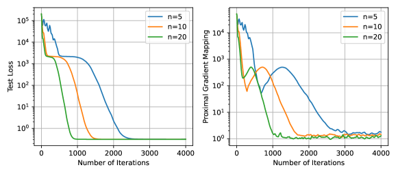
Figure 1: Linear-speedup performance of Prox-DASA for decentralized online sparse phase retrievel problems. (Prox-DASA-GT has relatively the same plots)

5.2 Real-World Data

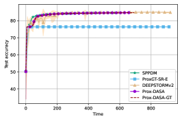
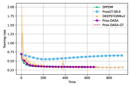
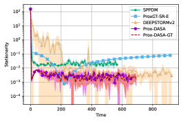
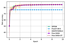
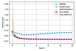
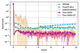
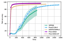
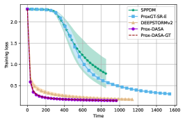
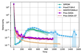
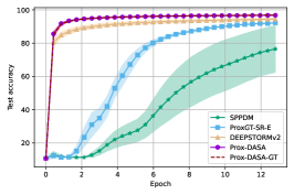
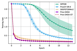
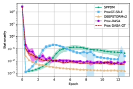
Figure 2: Comparisons between SPPDM (Wang et al., 2021), ProxGT-SR-E (Xin et al., 2021a), DEEPSTORM (Mancino-ball et al., 2023), Prox-DASA 1, and Prox-DASA-GT 2. The first two rows correspond to a9a and the last two rows correspond to MNIST. The results are averaged over 10 trials, and the shaded regions represent confidence intervals. The vertical axes in the third column are log-scale. It should be noted that ProxGT-SR-E maintains another hyperparameter $q$ (see, e.g., Algorithm 4 and Theorem 3 in (Xin et al., 2021a)) and computes gradients using a full batch every $q$ iterations. For simplicity, we do not include that amount of epochs when we plot this figure. In other words, the real number of epochs required to obtain a point on ProxGT-SR is larger than plotted in the figures in the second and fourth rows. We include the plots that take $q$ into account in Appendix.

Following Mancino-ball et al. (2023), we consider solving the classification problem

$$\underset{\theta\in\mathbb{R}^{d}}{\min}~{}\frac{1}{n}\sum_{i=1}^{n}\frac{1}{|\mathcal{D}_{i}|}\sum_{(x,y)\in\mathcal{D}_{i}}\ell_{i}(f(x;\theta),y)+\lambda\|\theta\|_{1},$$ (7)

on a9a and MNIST datasets. Here, $\ell_{i}$ denotes the cross-entropy loss, and $f$ represents a neural network parameterized by $\theta$ with $x$ being its input. $\mathcal{D}_{i}$ is the training set only available to agent $i$. The $L_{1}$ regularization term is used to impose a sparsity structure on the neural network. We use the code in Mancino-ball et al. (2023) for SPPDM, ProxGT-SR-O/E, DEEPSTORM, and then implement Prox-DASA and Prox-DASA-GT under their framework, which mainly utilizes PyTorch (Paszke et al., 2019) and mpi4py (Dalcin and Fang, 2021). We use a 2-layer perception model on a9a and the LeNet architecture (LeCun et al., 2015) for the MNIST dataset. We have 8 agents ($n=8$) which connect in the form of a ring for a9a and a random graph for MNIST. To demonstrate the performance of our algorithms in the constant batch size setting, the batch size is chosen to be 4 for a9a and 32 for MNIST for all algorithms. The learning rates provided in the code of Mancino-ball et al. (2023) are adjusted accordingly, and we select the ones with the best performance. For Prox-DASA and Prox-DASA-GT we choose a diminishing stepsize sequence, namely, $\alpha_{k}=\min\left\{\alpha\sqrt{\frac{n}{k}},1\right\}$ for all $k\geq 0$. Note that the same complexity (up to logarithmic factors) bounds can be obtained by directly plugging in the aforementioned expressions for $\alpha_{k}$ in Section 4.3. Then we tune $\gamma\in\left\{1,3,10\right\}$ and $\alpha\in\left\{0.3,1.0,3.0\right\}$. The penalty parameter $\lambda$ is chosen to be $0.0001$ for all experiments. The number of communication rounds per iteration $m$ is set to be $1$ for all algorithms. We evaluate the model performance periodically during training and then plot the results in Figure 2, from which we observe that both Prox-DASA and Prox-DASA-GT have considerably good performance with small variance in terms of test accuracy, training loss, and stationarity. In particular, it should be noted that although DEEPSTORM achieves better stationarity in Figure 2 and 2, training a neural network by using DEEPSTORM takes longer time than Prox-DASA and Prox-DASA-GT since it uses the momentum-based variance reduction technique, which requires two forward-backward passes (see, e.g., Eq. (10) and Algorithm 1 in Mancino-ball et al. (2023)) to compute the gradients in one iteration per agent. In contrast, ours only require one, which saves a large amount of time (see Table 1 in Appendix). We include further details of our experiments in the Appendix.

6 Conclusion

In this work, we propose and analyze a class of single time-scale decentralized proximal algorithms (Prox-DASA-(GT)) for non-convex stochastic composite optimization in the form of (1). We show that our algorithms achieve linear speed-up with respect to the number of agents using an $\mathcal{O}(1)$ batch size per iteration under mild assumptions. Furthermore, we demonstrate the efficiency and effectiveness of our algorithms through extensive experiments, in which our algorithms achieve relatively better results with less training time using a small batch size compared to existing methods. In future research, it would be intriguing to expand our work in the context of dependent and heavy-tailed stochastic gradient scenarios (Wai, 2020; Li and Liu, 2022).

Appendix A Experimental Details

All experiments are conducted on a laptop with Intel Core i7-11370H Processor and Windows 11 operating system. The total iteration numbers for a9a and MNIST are 10000 and 3000 respectively. The graph that represents the network topology is set to be ring (or cycle in graph theory) for a9a and random graph (given by Mancino-ball et al. [2023]) for MNIST (See Figure 3). To demonstrate the performance of our algorithms in a constant batch size setting, the batch sizes are chosen to be $4$ for a9a and $32$ for MNIST in all algorithms. We adjust the learning rates provided in the code of Mancino-ball et al. [2023] accordingly and select the ones that have the best performance. For Prox-DASA and Prox-DASA-GT we choose a diminishing stepsize sequence, namely, $\alpha_{k}=\min\left\{\alpha\sqrt{\frac{n}{k}},1\right\}$ for all $k\geq 0$. Note that the same complexity (up to logarithmic factors) bounds can be obtained by directly plugging in the aforementioned expressions for $\alpha_{k}$ in Section 4.3. Then we tune $\gamma\in\left\{1,3,10\right\}$ and $\alpha\in\left\{0.3,1.0,3.0\right\}$. The penalty parameter $\lambda$ is chosen to be $0.0001$ for all experiments.

We summarize the outputs of all experiments in Table 2, from which we can tell Prox-DASA and Prox-DASA-GT achieve good performance in a relatively short amount of time. The stationarity is defined as $\|\mathcal{G}(\bar{x}^{k},\nabla F(\bar{x}^{k}),1)\|^{2}+\|\mathbf{X}_{k}-\bar{\mathbf{X}}_{k}\|^{2}$, which is the same as that in Mancino-ball et al. [2023]. As mentioned in the caption of Figure 2 in the main paper, there is an extra hyperparameter $q$ in ProxGT-SR-E, and we found that large $q$ already works well for a9a experiment, but $q$ has to be small in the MNIST experiment otherwise the final accuracy will be much smaller than the one presented in Table 2. Hence in ProxGT-SR-E we choose $q=1000$ for a9a and $q=32$ for MNIST, and the plots that take this amount of epochs into account are in Figure 4.

Table 2: Comparisons between all algorithms

Algorithm	Accuracy	Training Loss	Stationarity	Communication time per iteration (s)	Computation time per iteration (s)	Total time per iteration (s)
a9a
SPPDM	84.64%	0.3340	0.0174	0.0260	0.0305	0.0565
ProxGT-SR-E	76.38%	0.6528	0.0797	0.0521	0.0394	0.0915
DEEPSTORM v2	84.90%	0.3274	0.0029	0.0525	0.0398	0.0923
Prox-DASA	84.71%	0.3338	0.0017	0.0360	0.0298	0.0658
Prox-DASA-GT	84.69%	0.3342	0.0017	0.0390	0.0301	0.0691
MNIST
SPPDM	76.54%	0.7854	0.0436	0.1587	0.1246	0.2833
ProxGT-SR-E	92.26%	0.3042	0.0250	0.1771	0.3368	0.5139
DEEPSTORM v2	94.52%	0.1759	0.0016	0.1758	0.2030	0.3788
Prox-DASA	96.74%	0.1469	0.0081	0.1912	0.1299	0.3211
Prox-DASA-GT	96.84%	0.1460	0.0058	0.1935	0.1317	0.3252

Figure 3: Network topology. The left represents the ring topology and the right represents (an instance of) the random graph.

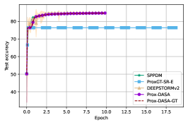
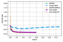
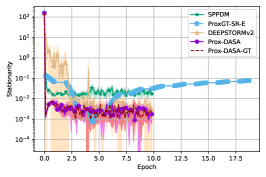
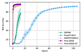
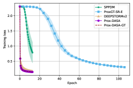
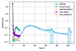
Figure 4: Comparisons between SPPDM [Wang et al., 2021], ProxGT-SR-E [Xin et al., 2021a], DEEPSTORM [Mancino-ball et al., 2023], Prox-DASA 1, and Prox-DASA-GT 2. In each experiment ProxGT-SR-E computes 1 more epoch than other algorithms every $q$ iterations. $q$ is chosen to be 1000 for a9a and 32 for MNIST.

Appendix B Accelerated Consensus

When the number of communication round $m>1$, we can replace $\mathbf{W}^{m}$ with the Chebyshev mixing protocol described in Algorithm 3. Then, we have the following lemma.

Lemma 1.

Suppose $\mathbf{W}$ satisfies Assumption 1. Let $\mathbf{A}_{0},\mathbf{A}_{m}$ be the input and output matrix of Algorithm 3 respectively. Then, we have

$$\left\|\mathbf{A}_{m}-\bar{\mathbf{A}}_{m}\right\|\leq 2\left(1-\sqrt{1-\rho}\right)^{m}\left\|\mathbf{A}_{0}-\bar{\mathbf{A}}_{0}\right\|.$$

Hence, we obtain a linear convergence rate of $\left(1-\sqrt{1-\rho}\right)$ instead of $\rho$. By virtue of that, we can set $m=\lceil\frac{1}{\sqrt{1-\rho}}\rceil$ to obtain a topology-independent iteration complexity.

Appendix C Convergence Analysis

We present the complete proof in this section. In the sequel, $\|\cdot\|$ denotes the $\ell_{2}$-norm for vectors and the Frobenius norm for matrices. $\|\cdot\|_{2}$ denotes the spectral norm for matrices. $\mathbf{1}$ represents the all-one vector. We identify vectors at agent $i$ in the subscript and use the superscript for the algorithm step. For example, the optimization variable of agent $i$ at step $k$ is denoted as $x^{k}_{i}$, and $z^{k}_{i}$ is the corresponding dual variable. We use uppercase bold letters to represent the matrix that collects all the variables from agents (corresponding lowercase) as columns. To be specific,

$$\mathbf{X}_{k}=\left[x_{1}^{k},\dots,x_{n}^{k}\right],\quad\mathbf{Z}_{k}=\left[z_{1}^{k},\dots,z_{n}^{k}\right],\quad\mathbf{Y}_{k}=\left[y_{1}^{k},\dots,y_{n}^{k}\right],\quad\mathbf{V}_{k+1}=\left[v^{k+1}_{1},\dots,v^{k+1}_{n}\right].$$

We add an overbar to a letter to denote the average over all agents. For example,

$$\bar{x}^{k}=\frac{1}{n}\sum_{i=1}^{n}x_{i}^{k}=\frac{1}{n}\mathbf{X}_{k}\mathbf{1},\quad\bar{\mathbf{X}}_{k}=[\bar{x}^{k},\dots,\bar{x}^{k}]=\bar{x}^{k}\mathbf{1}^{\top}=\frac{1}{n}\mathbf{X}_{k}\mathbf{1}\mathbf{1}^{\top}$$

Hence, the consensus errors for iterates $\{x^{k}_{i}\}$ and dual variables $\{z^{k}_{i}\}$ can be written as

$$\frac{1}{n}\sum_{i=1}^{n}\left\|x^{k}_{i}-\bar{x}^{k}\right\|^{2}=\frac{1}{n}\left\|\mathbf{X}_{k}-\bar{\mathbf{X}}_{k}\right\|^{2},\quad\frac{1}{n}\sum_{i=1}^{n}\left\|z^{k}_{i}-\bar{z}^{k}\right\|^{2}=\frac{1}{n}\left\|\mathbf{Z}_{k}-\bar{\mathbf{Z}}_{k}\right\|^{2}.$$

We denote $L_{\nabla F}=\underset{1\leq i\leq n}{\max}\{L_{\nabla F_{i}}\}$ for ease of presentation. Our proof heavily relies on the merit function below:

$$W(\bar{x}^{k},\bar{z}^{k})=\underbrace{\Phi(\bar{x}^{k})-\Phi_{*}}_{\text{function value gap}}+\underbrace{\Psi(\bar{x}^{k})-\eta(\bar{x}^{k},\bar{z}^{k})}_{\text{primal convergence}}+\lambda\underbrace{\left\|\nabla F(\bar{x}^{k})-\bar{z}^{k}\right\|^{2}}_{\text{dual convergence}},$$ (8)

where

$$\eta(x,z)=\min_{y\in\mathbb{R}^{d}}\left\{\left\langle z,y-x\right\rangle+\frac{1}{2\gamma}\|y-x\|^{2}+\Psi(y)\right\}.$$ (9)

C.1 Technical Lemmas

Lemma 2.

For any $p,q,r\in\mathbb{N}_{+}$ and matrix $\mathbf{A}\in\mathbb{R}^{p\times q},\mathbf{B}\in\mathbb{R}^{q\times r}$, we have:

$$\|\mathbf{A}\mathbf{B}\|\leq\min\left(\|\mathbf{A}\|_{2}\cdot\|\mathbf{B}\|,\|\mathbf{A}\|\cdot\|\mathbf{B}^{\top}\|_{2}\right).$$

Lemma 3.

Suppose $\mathbf{W}$ satisfies Assumption 1. For any $m\in\mathbb{N}_{+}$, we have

$$\left\|\mathbf{W}^{m}-\frac{\mathbf{1}_{n}\mathbf{1}^{\top}_{n}}{n}\right\|_{2}\leq\rho^{m}$$

Lemma 4.

Suppose we are given three sequences $\{a_{n}\}_{n=0}^{\infty},\{b_{n}\}_{n=0}^{\infty},\ \{\tau_{n}\}_{n=-1}^{\infty},$ and a constant $r$ satisfying

$$a_{k+1}\leq ra_{k}+b_{k},\ a_{k}\geq 0,\ b_{k}\geq 0,\ 0=\tau_{-1}\leq\tau_{k+1}\leq\tau_{k}\leq 1,$$ (10)

for all $k\geq 0$. Then for any $K>0$, we have

$$\sum_{k=0}^{K}\tau_{k}a_{k}\leq\frac{1}{1-r}\left(\tau_{0}a_{0}+\sum_{k=0}^{K}\tau_{k}b_{k}\right)$$

Proof.

Note that we have

$$(1-r)\sum_{k=0}^{K}\tau_{k}a_{k}\leq\sum_{k=0}^{K}\tau_{k}(a_{k}-a_{k+1}+b_{k})=\sum_{k=0}^{K}(\tau_{k}-\tau_{k-1})a_{k}-\tau_{K}a_{K+1}+\sum_{k=0}^{K}\tau_{k}b_{k}\leq\tau_{0}a_{0}+\sum_{k=0}^{K}\tau_{k}b_{k},$$

where the inequalities use (10), and the equality uses summation by parts. ∎

Lemma 5.

Let $\Psi:\mathbb{R}^{d}\rightarrow\mathbb{R}\cup\{+\infty\}$ be a closed proper convex function.

• Let $\eta(x,z)$ be the function defined in (9). Then, $\nabla\eta$ is $C_{\gamma}$-Lipschitz continuous where

  $$C_{\gamma}=2\sqrt{(1+\frac{1}{\gamma})^{2}+(1+\frac{\gamma}{2})^{2}}.$$ (11)

• For $x,z\in\mathbb{R}^{d}$ and $\gamma\in\mathbb{R}$, let $y_{+}=\operatorname{\mathbf{prox}}_{\Psi}^{\gamma}(x-\gamma z)=\underset{y\in\mathbb{R}^{d}}{\operatorname*{arg\,min\,}}\left\{\left\langle z,y-x\right\rangle+\frac{1}{2\gamma}\|y-x\|^{2}+\Psi(y)\right\}$, then for any $y\in\mathbb{R}^{d}$, we have

  $$\Psi(y_{+})-\Psi(y)\leq\left\langle z+\gamma^{-1}(y_{+}-x),y-y_{+}\right\rangle$$

Proof.

We prove (a) at first. Recall that the Moreau envelope of a convex and closed function $\Psi$ multiplied by a scalar $\gamma$ is defined by

$$\text{env}_{\gamma\Psi}(x)=\underset{y\in\mathbb{R}^{d}}{\min}\left\{\frac{1}{2\gamma}\left\|y-x\right\|^{2}+\Psi(y)\right\},$$

and its gradient is given by $\nabla\text{env}_{\gamma\Psi}(x)=\frac{1}{\gamma}(x-\operatorname{\mathbf{prox}}_{\Psi}^{\gamma}(x))$ where $\operatorname{\mathbf{prox}}_{\Psi}^{\gamma}(x)=\underset{y\in\mathbb{R}^{d}}{\operatorname*{arg\,min\,}}\left\{\frac{1}{2\gamma}\left\|y-x\right\|^{2}+\Psi(y)\right\}$. Note that $\eta(x,z)=\text{env}_{\gamma\Psi}\left(x-\gamma z\right)-\frac{\gamma}{2}\left\|z\right\|^{2}$. Therefore, the partial gradients of $\eta$ are given by

$$\nabla_{x}\eta(x,z)=-z-\gamma^{-1}\left(\operatorname{\mathbf{prox}}_{\Psi}^{\gamma}\left(x-\gamma z\right)-x\right),\quad\nabla_{z}\eta(x,z)=\operatorname{\mathbf{prox}}_{\Psi}^{\gamma}\left(x-\gamma z\right)-x.$$ (12)

Hence, for any $(x,z)$ and $(x^{\prime},z^{\prime})$,

$$\left\|\nabla\eta(x,z)-\nabla\eta(x^{\prime},z^{\prime})\right\| \leq\left\|\nabla_{x}\eta(x,z)-\nabla_{x}\eta(x^{\prime},z^{\prime})\right\|+\left\|\nabla_{z}\eta(x,z)-\nabla_{z}\eta(x^{\prime},z^{\prime})\right\|$$

$$\leq 2(1+1/\gamma)\left\|x-x^{\prime}\right\|+(2+\gamma)\left\|z-z^{\prime}\right\|\leq C_{\gamma}\left\|(x,z)-(x^{\prime},z^{\prime})\right\|.$$

To prove (b), denote the subdifferential of $\Psi(x)$ as $\partial\Psi(x)$. By the optimality condition, we have $\mathbf{0}$ is a subgradient of $H(y)=\left\langle z,y-x\right\rangle+\frac{1}{2\gamma}\|y-x\|^{2}+\Psi(y)$ at $y_{+}$, i.e.,

$$\mathbf{0}\in z+\gamma^{-1}(y_{+}-x)+\partial\Psi(y_{+}).$$

Hence, there exists a subgradient of $\Psi(y)$ at $y_{+}$, denoted by $\tilde{\nabla}\Psi(y_{+})$, such that

$$\tilde{\nabla}\Psi(y_{+})=-z-\gamma^{-1}(y_{+}-x).$$

Finally, by the convexity of $\Psi$, we have for any $y\in\mathbb{R}^{d}$,

$$\Psi(y)-\Psi(y_{+})\geq\left\langle\tilde{\nabla}\Psi(y_{+}),y-y_{+}\right\rangle=\left\langle-z-\gamma^{-1}(y_{+}-x),y-y_{+}\right\rangle,$$

which completes the proof. ∎

C.2 Building Blocks of Main Proof

The following lemma connects the consensus error of $\mathbf{Y}$ to the consensus errors of $\mathbf{X}$ and $\mathbf{Z}$.

Lemma 6.

Let $y^{k}_{+}=\operatorname{\mathbf{prox}}(\bar{x}^{k}-\gamma\bar{z}^{k})$. Then for any $k\geq 0$ and $\gamma>0$, we have

$$\left\|y^{k}_{+}-\bar{y}^{k}\right\|^{2}+\frac{1}{n}\left\|\mathbf{Y}_{k}-\bar{\mathbf{Y}}_{k}\right\|^{2}=\frac{1}{n}\sum_{i=1}^{n}\left\|y_{i}^{k}-y^{k}_{+}\right\|^{2}\leq\frac{2}{n}\left\{\|\mathbf{X}_{k}-\bar{\mathbf{X}}_{k}\|^{2}+\gamma^{2}\|\mathbf{Z}_{k}-\bar{\mathbf{Z}}_{k}\|^{2}\right\}.$$

Proof.

By the non-expansiveness of proximal operator, we have

$$\|y_{i}^{k}-y^{k}_{+}\|\leq\|x_{i}^{k}-\bar{x}^{k}-\gamma\left(z_{i}^{k}-\bar{z}^{k}\right)\|\leq\|x_{i}^{k}-\bar{x}^{k}\|+\gamma\|z_{i}^{k}-\bar{z}^{k}\|.$$ (13)

Hence we know the consensus error of $y$ can be bounded

$$\frac{1}{n}\|\mathbf{Y}_{k}-\bar{\mathbf{Y}}^{k}\|^{2}=\frac{1}{n}\sum_{i=1}^{n}\|y_{i}^{k}-\bar{y}^{k}\|^{2}=\frac{1}{n}\sum_{i=1}^{n}\|y_{i}^{k}-y^{k}_{+}+\frac{1}{n}\sum_{j=1}^{n}(y^{k}_{+}-y_{j}^{k})\|^{2}$$

$$= \frac{1}{n}\sum_{i=1}^{n}\|y_{i}^{k}-y^{k}_{+}\|^{2}-\|\frac{1}{n}\sum_{j=1}^{n}\left(y_{j}^{k}-y_{+}^{k}\right)\|^{2}\leq\frac{1}{n}\sum_{i=1}^{n}\|y_{i}^{k}-y^{k}_{+}\|^{2}$$

$$\leq \frac{2}{n}\left\{\|\mathbf{X}_{k}-\bar{\mathbf{X}}_{k}\|^{2}+\gamma^{2}\|\mathbf{Z}_{k}-\bar{\mathbf{Z}}_{k}\|^{2}\right\}$$ (14)

where the third equality uses the fact that

$$\frac{1}{n}\sum_{i=1}^{n}\left\|v_{i}-\left(\frac{1}{n}\sum_{j=1}^{n}v_{j}\right)\right\|^{2}=\frac{1}{n}\sum_{i=1}^{n}\left\|v_{i}\right\|^{2}-\left\|\frac{1}{n}\sum_{j=1}^{n}v_{j}\right\|^{2}$$

for any vectors $v_{i}\ (1\leq i\leq n)$. ∎

The following technical lemma explicitly characterizes the consensus error.

Lemma 7 (Conensus Error of Algorithm 1: Prox-DASA).

Suppose Assumptions 1, 4, 5, 6, and 7 hold. Let $\varrho(m)=\frac{(1+\rho^{2m})\rho^{2m}}{(1-\rho^{2m})^{2}}$, and $\rho,m$ and $\alpha_{k}$ satisfy

$$\varrho(m)\alpha_{k}^{2}\leq\min\left\{\frac{1}{8},\frac{1}{24L_{\nabla F}^{2}\gamma^{2}}\right\},\ 0=\alpha_{-1}\leq\alpha_{k+1}\leq\alpha_{k}\leq 1$$ (15)

for any $k\geq 0$. Then in Algorithm 1 for any $p\geq 0$, we have

$$\sum_{k=0}^{K}\frac{\alpha_{k}^{p}}{n}\mathbb{E}\left[\|\mathbf{X}_{k}-\bar{\mathbf{X}}_{k}\|^{2}\right]\leq 4\gamma^{2}(\sigma^{2}+3L_{\nabla F}^{2}\nu^{2})\varrho(m)\sum_{k=0}^{K}\alpha_{k}^{p+2},$$

$$\sum_{k=0}^{K}\frac{\alpha_{k}^{p}}{n}\mathbb{E}\left[\|\mathbf{Z}_{k}-\bar{\mathbf{Z}}_{k}\|^{2}\right]\leq 4(\sigma^{2}+3L_{\nabla F}^{2}\nu^{2})\varrho(m)\sum_{k=0}^{K}\alpha_{k}^{p+2},.$$

Proof.

By Assumption 1, the iterates in Algorithm 1 satisfy

$$\mathbf{X}_{k+1}=(1-\alpha_{k})\mathbf{X}_{k}\mathbf{W}^{m}+\alpha_{k}\mathbf{Y}_{k}\mathbf{W}^{m},\ \bar{x}^{k+1}=(1-\alpha_{k})\bar{x}^{k}+\alpha_{k}\bar{y}^{k},$$ (16)

$$\mathbf{Z}_{k+1}=(1-\alpha_{k})\mathbf{Z}_{k}\mathbf{W}^{m}+\alpha_{k}\mathbf{V}_{k+1}\mathbf{W}^{m},\ \bar{z}^{k+1}=(1-\alpha_{k})\bar{z}^{k}+\alpha_{k}\bar{v}^{k+1}.$$

Hence, for the consensus error of iterates $\{x^{k}_{i}\}$, we have

$$\left\|\mathbf{X}_{k+1}-\bar{\mathbf{X}}_{k+1}\right\|^{2}$$

$$= \left\|\bigg{(}(1-\alpha_{k})\left(\mathbf{X}_{k}-\bar{\mathbf{X}}_{k}\right)+\alpha_{k}\left(\mathbf{Y}_{k}-\bar{\mathbf{Y}}_{k}\right)\bigg{)}\left(\mathbf{W}^{m}-\frac{\mathbf{1}\mathbf{1}^{\top}}{n}\right)\right\|^{2}$$

$$\leq \left\{\left(1+\frac{1-\rho^{2m}}{2\rho^{2m}}\right)(1-\alpha_{k})^{2}\left\|\mathbf{X}_{k}-\bar{\mathbf{X}}_{k}\right\|^{2}+\left(1+\frac{2\rho^{2m}}{1-\rho^{2m}}\right)\alpha_{k}^{2}\left\|\mathbf{Y}_{k}-\bar{\mathbf{Y}}_{k}\right\|^{2}\right\}\rho^{2m}$$

$$\leq \frac{(1+\rho^{2m})}{2}\left\|\mathbf{X}_{k}-\bar{\mathbf{X}}_{k}\right\|^{2}+\frac{(1+\rho^{2m})\rho^{2m}}{1-\rho^{2m}}\alpha_{k}^{2}\left\|\mathbf{Y}_{k}-\bar{\mathbf{Y}}_{k}\right\|^{2},$$ (17)

where the first inequality uses Lemma 2 and 3. Combining (15), (17), and Lemma 6, we have

$$\mathbb{E}\left[\|\mathbf{X}_{k+1}-\bar{\mathbf{X}}_{k+1}\|^{2}\right] \leq\frac{(1+\rho^{2m})}{2}\mathbb{E}\left[\|\mathbf{X}_{k}-\bar{\mathbf{X}}_{k}\|^{2}\right]+\frac{(1-\rho^{2m})}{4}\mathbb{E}\left[\|\mathbf{X}_{k}-\bar{\mathbf{X}}_{k}\|^{2}+\gamma^{2}\|\mathbf{Z}_{k}-\bar{\mathbf{Z}}_{k}\|^{2}\right]$$

$$=\frac{(3+\rho^{2m})}{4}\mathbb{E}\left[\|\mathbf{X}_{k}-\bar{\mathbf{X}}_{k}\|^{2}\right]+\frac{(1-\rho^{2m})\gamma^{2}}{4}\mathbb{E}\left[\|\mathbf{Z}_{k}-\bar{\mathbf{Z}}_{k}\|^{2}\right]$$

Using Lemma 4 in the above inequality with $\tau_{k}=\frac{\alpha_{k}^{p}}{n}$ for any fixed $p\geq 0$ we know

$$\sum_{k=0}^{K}\frac{\alpha_{k}^{p}}{n}\mathbb{E}\left[\|\mathbf{X}_{k}-\bar{\mathbf{X}}_{k}\|^{2}\right]\leq\sum_{k=0}^{K}\frac{\gamma^{2}\alpha_{k}^{p}}{n}\mathbb{E}\left[\|\mathbf{Z}_{k}-\bar{\mathbf{Z}}_{k}\|^{2}\right].$$ (18)

Similarly to (17), we can obtain the following results on the consensus error of dual variables $\{z^{k}_{i}\}$:

$$\left\|\mathbf{Z}_{k+1}-\bar{\mathbf{Z}}_{k+1}\right\|^{2}\leq\frac{(1+\rho^{2m})}{2}\left\|\mathbf{Z}_{k}-\bar{\mathbf{Z}}_{k}\right\|^{2}+\frac{(1+\rho^{2m})\rho^{2m}}{1-\rho^{2m}}\alpha_{k}^{2}\left\|\mathbf{V}_{k+1}-\bar{\mathbf{V}}_{k+1}\right\|^{2},$$ (19)

Using (15) and Lemma 4 in (19) with $\tau_{k}=\frac{\alpha_{k}^{p}}{n}$, we have

$$\sum_{k=0}^{K}\frac{\alpha_{k}^{p}}{n}\mathbb{E}\left[\|\mathbf{Z}_{k}-\bar{\mathbf{Z}}_{k}\|^{2}\right]\leq 2\varrho(m)\sum_{k=0}^{K}\frac{\alpha_{k}^{p+2}}{n}\mathbb{E}\left[\|\mathbf{V}_{k+1}-\bar{\mathbf{V}}_{k+1}\|^{2}\right].$$ (20)

To bound $\|\mathbf{V}_{k+1}-\bar{\mathbf{V}}_{k+1}\|$ we first notice that

$$v_{i}^{k+1}-\bar{v}^{k+1}= v_{i}^{k+1}-\mathbb{E}\left[v_{i}^{k+1}|\mathscr{F}_{k}\right]-\frac{1}{n}\sum_{j=1}^{n}(v_{j}^{k+1}-\mathbb{E}\left[v_{j}^{k+1}|\mathscr{F}_{k}\right])$$

$$+ \mathbb{E}\left[v_{i}^{k+1}|\mathscr{F}_{k}\right]-\nabla F_{i}(\bar{x}^{k})+\nabla F_{i}(\bar{x}^{k})-\nabla F(\bar{x}^{k})+\nabla F(\bar{x}^{k})-\frac{1}{n}\sum_{j=1}^{n}\mathbb{E}\left[v_{j}^{k+1}|\mathscr{F}_{k}\right]$$

$$= \left(1-\frac{1}{n}\right)(v_{i}^{k+1}-\mathbb{E}\left[v_{i}^{k+1}|\mathscr{F}_{k}\right])-\frac{1}{n}\sum_{j\neq i}(v_{j}^{k+1}-\mathbb{E}\left[v_{j}^{k+1}|\mathscr{F}_{k}\right])$$

$$+ \left(1-\frac{1}{n}\right)\left(\nabla F_{i}(x_{i}^{k})-\nabla F_{i}(\bar{x}^{k})\right)+\nabla F_{i}(\bar{x}^{k})-\nabla F(\bar{x}^{k})+\frac{1}{n}\sum_{j\neq i}\left(\nabla F_{j}(\bar{x}^{k})-\nabla F_{i}(x_{j}^{k})\right)$$

which gives

$$\mathbb{E}\left[\|v_{i}^{k+1}-\bar{v}^{k+1}\|^{2}\right]$$

$$= \left(1-\frac{1}{n}\right)^{2}\mathbb{E}\left[\|v_{i}^{k+1}-\mathbb{E}\left[v_{i}^{k+1}|\mathscr{F}_{k}\right]\|^{2}\right]+\frac{1}{n^{2}}\sum_{j\neq i}^{n}\mathbb{E}\left[\|v_{j}^{k+1}-\mathbb{E}\left[v_{j}^{k+1}|\mathscr{F}_{k}\right]\|^{2}\right]$$

$$+ \left\|\left(1-\frac{1}{n}\right)\left(\nabla F_{i}(x_{i}^{k})-\nabla F_{i}(\bar{x}^{k})\right)+\nabla F_{i}(\bar{x}^{k})-\nabla F(\bar{x}^{k})+\frac{1}{n}\sum_{j\neq i}\left(\nabla F_{j}(\bar{x}^{k})-\nabla F_{i}(x_{j}^{k})\right)\right\|^{2}$$

$$\leq \sigma^{2}+3L_{\nabla F}^{2}\left(\left(1-\frac{1}{n}\right)^{2}\|x_{i}^{k}-\bar{x}^{k}\|^{2}+\nu^{2}+\frac{1}{n}\sum_{j\neq i}\|x_{j}^{k}-\bar{x}^{k}\|^{2}\right),$$

where the first equality uses Assumption 5, and the second inequality uses Cauchy-Schwarz inequality, Assumptions 2, 6, and 7. Hence we have

$$\mathbb{E}\left[\|\mathbf{V}_{k+1}-\bar{\mathbf{V}}_{k+1}\|^{2}\right]\leq 6L_{\nabla F}^{2}\mathbb{E}\left[\|\mathbf{X}_{k}-\bar{\mathbf{X}}_{k}\|^{2}\right]+n\sigma^{2}+3nL_{\nabla F}^{2}\nu^{2}.$$ (21)

Combining (20) and (21), we have

$$\sum_{k=0}^{K}\frac{\alpha_{k}^{p}}{n}\mathbb{E}\left[\|\mathbf{Z}_{k}-\bar{\mathbf{Z}}_{k}\|^{2}\right]\leq 2\varrho(m)\sum_{k=0}^{K}\left\{\frac{6L_{\nabla F}^{2}\alpha_{k}^{p+2}}{n}\mathbb{E}\left[\|\mathbf{X}_{k}-\bar{\mathbf{X}}_{k}\|^{2}\right]+(\sigma^{2}+3L_{\nabla F}^{2}\nu^{2})\sum_{k=0}^{K}\alpha_{k}^{p+2}\right\}$$ (22)

$$\leq \sum_{k=0}^{K}\left\{12\varrho(m)\alpha_{k}^{2}L_{\nabla F}^{2}\gamma^{2}\right\}\frac{\alpha_{k}^{p}}{n\gamma^{2}}\mathbb{E}\left[\|\mathbf{X}_{k}-\bar{\mathbf{X}}_{k}\|^{2}\right]+2(\sigma^{2}+3L_{\nabla F}^{2}\nu^{2})\varrho(m)\sum_{k=0}^{K}\alpha_{k}^{p+2}$$

$$\leq \sum_{k=0}^{K}\frac{\alpha_{k}^{p}}{2n}\mathbb{E}\left[\|\mathbf{Z}_{k}-\bar{\mathbf{Z}}_{k}\|^{2}\right]+2(\sigma^{2}+3L_{\nabla F}^{2}\nu^{2})\varrho(m)\sum_{k=0}^{K}\alpha_{k}^{p+2},$$

where the second inequality uses (15). By (18) and (22) we can finally obtain that

$$\sum_{k=0}^{K}\frac{\alpha_{k}^{p}}{n}\mathbb{E}\left[\|\mathbf{X}_{k}-\bar{\mathbf{X}}_{k}\|^{2}\right]\leq 4\gamma^{2}(\sigma^{2}+3L_{\nabla F}^{2}\nu^{2})\varrho(m)\sum_{k=0}^{K}\alpha_{k}^{p+2},,$$ (23)

$$\sum_{k=0}^{K}\frac{\alpha_{k}^{p}}{n}\mathbb{E}\left[\|\mathbf{Z}_{k}-\bar{\mathbf{Z}}_{k}\|^{2}\right]\leq 4(\sigma^{2}+3L_{\nabla F}^{2}\nu^{2})\varrho(m)\sum_{k=0}^{K}\alpha_{k}^{p+2},.$$ (24)

∎

Lemma 8 (Conensus Error of Algorithm 2: Prox-DASA-GT).

Suppose Assumptions 1, 4, 6 and 5 hold. Let $\varrho(m)=\frac{(1+\rho^{2m})\rho^{2m}}{(1-\rho^{2m})^{2}}$, and $\rho,m$ and $\alpha_{k}$ satisfy

$$\varrho(m)\alpha_{k}^{2}\leq\frac{1}{8},\ \varrho(m)\alpha_{k}\leq\frac{1}{9L_{\nabla F}\gamma},\ 0=\alpha_{-1}\leq\alpha_{k+1}\leq\alpha_{k}\leq 1$$ (25)

for any $k\geq 0$, and the initialization satisfies $u_{i}^{0}=v_{i}^{0}=0$ for all $i$. Then in Algorithm 2 for any $p\geq 0$ we have

$$\sum_{k=0}^{K}\frac{\alpha_{k}^{p}}{n}\mathbb{E}\left[\|\mathbf{X}_{k}-\bar{\mathbf{X}}_{k}\|^{2}\right]\leq 40\gamma^{2}\varrho(m)^{2}\sum_{k=0}^{K}\alpha_{k}^{p+2}\left\{L_{\nabla F}^{2}\alpha_{k}^{2}\mathbb{E}\left[\|\bar{x}^{k}-\bar{y}^{k}\|^{2}\right]+2\sigma^{2}\right\},$$

$$\sum_{k=0}^{K}\frac{\alpha_{k}^{p}}{n}\mathbb{E}\left[\|\mathbf{Z}_{k}-\bar{\mathbf{Z}}_{k}\|^{2}\right]\leq 40\varrho(m)^{2}\sum_{k=0}^{K}\alpha_{k}^{p+2}\left\{L_{\nabla F}^{2}\alpha_{k}^{2}\mathbb{E}\left[\|\bar{x}^{k}-\bar{y}^{k}\|^{2}\right]+2\sigma^{2}\right\}.$$

Proof.

The updates in Algorithm 2 take the form:

$$\mathbf{X}_{k+1}=(1-\alpha_{k})\mathbf{X}_{k}\mathbf{W}^{m}+\alpha_{k}\mathbf{Y}_{k}\mathbf{W}^{m},\ \bar{x}^{k+1}=(1-\alpha_{k})\bar{x}^{k}+\alpha_{k}\bar{y}^{k},$$ (26)

$$\mathbf{U}_{k+1}=\mathbf{U}_{k}\mathbf{W}^{m}+(\mathbf{V}_{k+1}-\mathbf{V}_{k})\mathbf{W}^{m},\ \bar{u}^{k+1}=\bar{u}^{k}+\bar{v}^{k+1}-\bar{v}^{k},$$

$$\mathbf{Z}_{k+1}=(1-\alpha_{k})\mathbf{Z}_{k}\mathbf{W}^{m}+\alpha_{k}\mathbf{U}_{k}\mathbf{W}^{m},\ \bar{z}^{k+1}=(1-\alpha_{k})\bar{z}^{k}+\alpha_{k}\bar{u}^{k}.$$

Setting $u_{i}^{0}=v_{i}^{0}$, we can prove by induction that $\bar{u}^{k}=\bar{v}^{k}$. To analyze the consensus error of $\mathbf{U}_{k}$, we first notice:

$$\mathbf{U}_{k+1}-\bar{\mathbf{U}}_{k+1}$$

$$= \left(\mathbf{U}_{k}-\bar{\mathbf{U}}_{k}+\mathbf{V}_{k+1}-\mathbf{V}_{k}-\bar{\mathbf{V}}^{k+1}+\bar{\mathbf{V}}^{k}\right)\left(\mathbf{W}^{m}-\frac{\mathbf{1}\mathbf{1}^{\top}}{n}\right)$$

$$= \left(\mathbf{U}_{k}-\bar{\mathbf{U}}_{k}+\left(\mathbf{V}_{k+1}-\mathbf{V}_{k}\right)\left(\mathbf{I}-\frac{\mathbf{1}\mathbf{1}^{\top}}{n}\right)\right)\left(\mathbf{W}^{m}-\frac{\mathbf{1}\mathbf{1}^{\top}}{n}\right)$$

which gives

$$\|\mathbf{U}_{k+1}-\bar{\mathbf{U}}_{k+1}\|^{2}$$

$$\leq \left\{\left(1+\frac{1-\rho^{2m}}{2\rho^{2m}}\right)\left\|\mathbf{U}_{k}-\bar{\mathbf{U}}_{k}\right\|^{2}+\left(1+\frac{2\rho^{2m}}{1-\rho^{2m}}\right)\left\|\mathbf{V}_{k+1}-\mathbf{V}_{k}\right\|^{2}\right\}\rho^{2m}$$

$$= \frac{(1+\rho^{2m})}{2}\left\|\mathbf{U}_{k}-\bar{\mathbf{U}}_{k}\right\|^{2}+\frac{(1+\rho^{2m})\rho^{2m}}{1-\rho^{2m}}\left\|\mathbf{V}_{k+1}-\mathbf{V}_{k}\right\|^{2}.$$

Using Lemma 4, we know for any $k\geq 0$ and $p\geq 0$,

$$\sum_{k=0}^{K}\alpha_{k}^{p}\|\mathbf{U}_{k}-\bar{\mathbf{U}}_{k}\|^{2}\leq 2\varrho(m)\sum_{k=0}^{K}\alpha_{k}^{p}\left\|\mathbf{V}_{k+1}-\mathbf{V}_{k}\right\|^{2}.$$ (27)

Note that we also have

$$\mathbf{V}_{k+1}-\mathbf{V}_{k}= \mathbf{V}_{k+1}-\mathbb{E}\left[\mathbf{V}_{k+1}|\mathscr{F}_{k}\right]-\left(\mathbf{V}_{k}-\mathbb{E}\left[\mathbf{V}_{k}|\mathscr{F}_{k-1}\right]\right)$$

$$+\mathbb{E}\left[\mathbf{V}_{k+1}|\mathscr{F}_{k}\right]-\nabla\mathbf{F}(\bar{x}^{k})+\nabla\mathbf{F}(\bar{x}^{k})-\nabla\mathbf{F}(\bar{x}^{k-1})+\nabla\mathbf{F}(\bar{x}^{k-1})-\mathbb{E}\left[\mathbf{V}_{k}|\mathscr{F}_{k-1}\right]$$

where we overload the notation and define $\nabla\mathbf{F}(x)=[\nabla F_{1}(x),...,\nabla F_{n}(x)]$. Hence we know

$$\mathbb{E}\left[\|\mathbf{V}_{k+1}-\mathbf{V}_{k}\|^{2}\right]$$ (28)

$$\leq 5\bigg{\{}\mathbb{E}\left[\|\mathbf{V}_{k+1}-\mathbb{E}\left[\mathbf{V}_{k+1}|\mathscr{F}_{k}\right]\|^{2}\right]+\mathbb{E}\left[\|\mathbf{V}_{k}-\mathbb{E}\left[\mathbf{V}_{k}|\mathscr{F}_{k-1}\right]\|^{2}\right]+\mathbb{E}\left[\sum_{i=1}^{n}\|\nabla F_{i}(x_{i}^{k})-\nabla F_{i}(\bar{x}^{k})\|^{2}\right]$$

$$+ \mathbb{E}\left[\sum_{i=1}^{n}\|\nabla F_{i}(\bar{x}^{k})-\nabla F_{i}(\bar{x}^{k-1})\|^{2}\right]+\mathbb{E}\left[\sum_{i=1}^{n}\|\nabla F_{i}(x_{i}^{k-1})-\nabla F_{i}(\bar{x}^{k-1})\|^{2}\right]\bigg{\}}$$

$$\leq 5\left(2n\sigma^{2}+L_{\nabla F}^{2}\mathbb{E}\left[\|\mathbf{X}_{k}-\bar{\mathbf{X}}_{k}\|^{2}+\|\mathbf{X}^{k-1}-\bar{\mathbf{X}}^{k-1}\|^{2}+n\alpha_{k-1}^{2}\|\bar{x}^{k-1}-\bar{y}^{k-1}\|^{2}\right]\right)$$

where the first inequality uses Cauchy-Schwarz inequality, and the second inequality uses Lipschitz continuity of $\nabla f_{i}$ and (26). For simplicity we set $x_{i}^{-1}=y_{i}^{-1}=0$ for all $i$ so that it is easy to check the above inequality holds for all $k\geq 0$. Using (27) and (28) we know:

$$\sum_{k=0}^{K}\frac{\alpha_{k}^{p}}{n}\|\mathbf{U}_{k}-\bar{\mathbf{U}}_{k}\|^{2}$$ (29)

$$\leq \frac{10\varrho(m)}{n}\sum_{k=0}^{K}\alpha_{k}^{p}\left(2n\sigma^{2}+L_{\nabla F}^{2}\mathbb{E}\left[\|\mathbf{X}_{k}-\bar{\mathbf{X}}_{k}\|^{2}+\|\mathbf{X}^{k-1}-\bar{\mathbf{X}}^{k-1}\|^{2}+n\alpha_{k-1}^{2}\|\bar{x}^{k-1}-\bar{y}^{k-1}\|^{2}\right]\right).$$

$$\leq \frac{20L_{\nabla F}^{2}\varrho(m)}{n}\sum_{k=0}^{K}\alpha_{k}^{p}\mathbb{E}\left[\|\mathbf{X}_{k}-\bar{\mathbf{X}}_{k}\|^{2}\right]+10L_{\nabla F}^{2}\varrho(m)\sum_{k=0}^{K}\alpha_{k}^{p+2}\mathbb{E}\left[\|\bar{x}^{k}-\bar{y}^{k}\|^{2}\right]+20\sigma^{2}\varrho(m)\sum_{k=0}^{K}\alpha_{k}^{p},$$ (30)

where the third inequality uses (25). For other consensus error terms we follow the same proof in Lemma 7 to get

$$\left\|\mathbf{X}_{k+1}-\bar{\mathbf{X}}_{k+1}\right\|^{2}\leq\frac{(1+\rho^{2m})}{2}\left\|\mathbf{X}_{k}-\bar{\mathbf{X}}_{k}\right\|^{2}+\frac{(1+\rho^{2m})\rho^{2m}}{1-\rho^{2m}}\alpha_{k}^{2}\left\|\mathbf{Y}_{k}-\bar{\mathbf{Y}}_{k}\right\|^{2},$$ (31)

$$\left\|\mathbf{Y}_{k}-\bar{\mathbf{Y}}_{k}\right\|^{2}\leq 2(\left\|\mathbf{X}_{k}-\bar{\mathbf{X}}_{k}\right\|^{2}+\gamma^{2}\left\|\mathbf{Z}_{k}-\bar{\mathbf{Z}}_{k}\right\|^{2}),$$ (32)

$$\left\|\mathbf{Z}_{k+1}-\bar{\mathbf{Z}}_{k+1}\right\|^{2}\leq\frac{(1+\rho^{2m})}{2}\left\|\mathbf{Z}_{k}-\bar{\mathbf{Z}}_{k}\right\|^{2}+\frac{(1+\rho^{2m})\rho^{2m}}{1-\rho^{2m}}\alpha_{k}^{2}\left\|\mathbf{U}_{k}-\bar{\mathbf{U}}_{k}\right\|^{2}.$$ (33)

Hence we know (18) still holds:

$$\sum_{k=0}^{K}\frac{\alpha_{k}^{p}}{n}\mathbb{E}\left[\|\mathbf{X}_{k}-\bar{\mathbf{X}}_{k}\|^{2}\right]\leq\sum_{k=0}^{K}\frac{\gamma^{2}\alpha_{k}^{p}}{n}\mathbb{E}\left[\|\mathbf{Z}_{k}-\bar{\mathbf{Z}}_{k}\|^{2}\right].$$ (34)

Applying Lemma (4) in (33) with $\tau_{k}=\frac{\alpha_{k}^{p}}{n}$, we have

$$\sum_{k=0}^{K}\frac{\alpha_{k}^{p}}{n}\mathbb{E}\left[\|\mathbf{Z}_{k}-\bar{\mathbf{Z}}_{k}\|^{2}\right]\leq 2\varrho(m)\sum_{k=0}^{K}\frac{\alpha_{k}^{p+2}}{n}\mathbb{E}\left[\|\mathbf{U}_{k}-\bar{\mathbf{U}}_{k}\|^{2}\right].$$ (35)

The above two inequalities together with (30) and (25) imply

$$\sum_{k=0}^{K}\frac{\alpha_{k}^{p}}{n}\mathbb{E}\left[\|\mathbf{X}_{k}-\bar{\mathbf{X}}_{k}\|^{2}\right]\leq 2\varrho(m)\gamma^{2}\sum_{k=0}^{K}\frac{\alpha_{k}^{p+2}}{n}\mathbb{E}\left[\|\mathbf{U}_{k}-\bar{\mathbf{U}}_{k}\|^{2}\right]$$

$$\leq \sum_{k=0}^{K}\left\{40L_{\nabla F}^{2}\gamma^{2}\varrho(m)^{2}\alpha_{k}^{2}\right\}\frac{\alpha_{k}^{p}}{n}\mathbb{E}\left[\|\mathbf{X}_{k}-\bar{\mathbf{X}}_{k}\|^{2}\right]+20\gamma^{2}\varrho(m)^{2}\sum_{k=0}^{K}\alpha_{k}^{p+2}\left\{L_{\nabla F}^{2}\alpha_{k}^{2}\mathbb{E}\left[\|\bar{x}^{k}-\bar{y}^{k}\|^{2}\right]+2\sigma^{2}\right\}$$

$$\leq \frac{1}{2}\sum_{k=0}^{K}\frac{\alpha_{k}^{p}}{n}\mathbb{E}\left[\|\mathbf{X}_{k}-\bar{\mathbf{X}}_{k}\|^{2}\right]+20\gamma^{2}\varrho(m)^{2}\sum_{k=0}^{K}\alpha_{k}^{p+2}\left\{L_{\nabla F}^{2}\alpha_{k}^{2}\mathbb{E}\left[\|\bar{x}^{k}-\bar{y}^{k}\|^{2}\right]+2\sigma^{2}\right\},$$

which gives

$$\sum_{k=0}^{K}\frac{\alpha_{k}^{p}}{n}\mathbb{E}\left[\|\mathbf{X}_{k}-\bar{\mathbf{X}}_{k}\|^{2}\right]\leq 40\gamma^{2}\varrho(m)^{2}\sum_{k=0}^{K}\alpha_{k}^{p+2}\left\{L_{\nabla F}^{2}\alpha_{k}^{2}\mathbb{E}\left[\|\bar{x}^{k}-\bar{y}^{k}\|^{2}\right]+2\sigma^{2}\right\}.$$ (36)

Combining (25), (30), (35), and (36), we obtain that

$$\sum_{k=0}^{K}\frac{\alpha_{k}^{p}}{n}\mathbb{E}\left[\|\mathbf{Z}_{k}-\bar{\mathbf{Z}}_{k}\|^{2}\right]\leq 2\varrho(m)\sum_{k=0}^{K}\frac{\alpha_{k}^{p+2}}{n}\mathbb{E}\left[\|\mathbf{U}_{k}-\bar{\mathbf{U}}_{k}\|^{2}\right]$$

$$\leq \frac{1}{2\gamma^{2}}\sum_{k=0}^{K}\frac{\alpha_{k}^{p}}{n}\mathbb{E}\left[\|\mathbf{X}_{k}-\bar{\mathbf{X}}_{k}\|^{2}\right]+20\varrho(m)^{2}\sum_{k=0}^{K}\alpha_{k}^{p+2}\left\{L_{\nabla F}^{2}\alpha_{k}^{2}\mathbb{E}\left[\|\bar{x}^{k}-\bar{y}^{k}\|^{2}\right]+2\sigma^{2}\right\},$$

$$\leq 40\varrho(m)^{2}\sum_{k=0}^{K}\alpha_{k}^{p+2}\left\{L_{\nabla F}^{2}\alpha_{k}^{2}\mathbb{E}\left[\|\bar{x}^{k}-\bar{y}^{k}\|^{2}\right]+2\sigma^{2}\right\}.$$

∎

Lemma 9 (Basic Inequalities of Dual Convergence).

$$\begin{split}\delta^{k}&=\frac{\nabla F(\bar{x}^{k})-\nabla F(\bar{x}^{k+1})}{\alpha_{k}}+\frac{1}{n}\sum_{i=1}^{n}\nabla F_{i}(x^{k}_{i})-\nabla F(\bar{x}^{k}),\quad\bar{\Delta}^{k+1}=\bar{v}^{k+1}-\frac{1}{n}\sum_{i=1}^{n}\nabla F_{i}(x^{k}_{i}).\end{split}$$ (37)

Under Assumption 2, we have

$$\begin{split}\|\bar{z}^{k+1}-&\nabla F(\bar{x}^{k+1})\|^{2}\leq(1-\alpha_{k})\left\|\bar{z}^{k}-\nabla F(\bar{x}^{k})\right\|^{2}+2L_{\nabla F}^{2}\alpha_{k}\left\|\bar{x}^{k}-\bar{y}^{k}\right\|^{2}+\alpha_{k}^{2}\left\|\bar{\Delta}^{k+1}\right\|^{2}\\ &+\frac{2L_{\nabla F}^{2}\alpha_{k}}{n}\left\|\mathbf{X}_{k}-\bar{\mathbf{X}}_{k}\right\|^{2}+2\left\langle\alpha_{k}\bar{\Delta}^{k+1},(1-\alpha_{k})\left(\bar{z}^{k}-\nabla F(\bar{x}^{k})\right)+\alpha_{k}\delta^{k}\right\rangle,\end{split}$$ (38)

and

$$\begin{split}\left\|\bar{z}^{k+1}-\bar{z}^{k}\right\|^{2}&\leq\alpha_{k}^{2}\bigg{\{}2\left\|\nabla F(\bar{x}^{k})-\bar{z}^{k}\right\|^{2}+\frac{2L_{\nabla F}^{2}}{n}\left\|\mathbf{X}_{k}-\bar{\mathbf{X}}_{k}\right\|^{2}+\left\|\bar{\Delta}^{k+1}\right\|^{2}\\ &\hskip 160.00024pt+2\left\langle\bar{\Delta}^{k+1},\frac{1}{n}\sum_{i=1}^{n}\nabla F_{i}(x^{k}_{i})-\bar{z}^{k}\right\rangle\bigg{\}}.\end{split}$$ (39)

Proof.

By definitions in (37), we have

$$\bar{z}^{k+1}-\nabla F(\bar{x}^{k+1})=(1-\alpha_{k})\left(\bar{z}^{k}-\nabla F(\bar{x}^{k})\right)+\alpha_{k}\delta^{k}+\alpha_{k}\bar{\Delta}^{k+1},$$

Hence, we can get

$$\left\|\bar{z}^{k+1}-\nabla F(\bar{x}^{k+1})\right\|^{2}$$

$$=\left\|(1-\alpha_{k})\left(\bar{z}^{k}-\nabla F(\bar{x}^{k})\right)+\alpha_{k}\delta^{k}\right\|^{2}+\alpha_{k}^{2}\left\|\bar{\Delta}^{k+1}\right\|^{2}+2\left\langle\alpha_{k}\bar{\Delta}^{k+1},(1-\alpha_{k})\left(\bar{z}^{k}-\nabla F(\bar{x}^{k})\right)+\alpha_{k}\delta^{k}\right\rangle$$

$$\leq(1-\alpha_{k})\left\|\bar{z}^{k}-\nabla F(\bar{x}^{k})\right\|^{2}+\alpha_{k}\left\|\delta^{k}\right\|^{2}+\alpha_{k}^{2}\left\|\bar{\Delta}^{k+1}\right\|^{2}+2\left\langle\alpha_{k}\bar{\Delta}^{k+1},(1-\alpha_{k})\left(\bar{z}^{k}-\nabla F(\bar{x}^{k})\right)+\alpha_{k}\delta^{k}\right\rangle$$

where the inequality uses the convexity of $\|\cdot\|^{2}$. In addition, we have

$$\left\|\delta^{k}\right\|^{2} \leq 2\left\|\frac{\nabla F(\bar{x}^{k})-\nabla F(\bar{x}^{k+1})}{\alpha_{k}}\right\|^{2}+2\left\|\frac{1}{n}\sum_{i=1}^{n}\left(\nabla F_{i}(x_{i}^{k})-\nabla F_{i}(\bar{x}^{k})\right)\right\|^{2}$$

$$\leq 2L_{\nabla F}^{2}\left\|\bar{x}^{k}-\bar{y}^{k}\right\|^{2}+\frac{2L_{\nabla F}^{2}}{n}\left\|\mathbf{X}_{k}-\bar{\mathbf{X}}_{k}\right\|^{2},$$

which completes the proof of (38). The inequality (39) can be proved similarly by noting that

$$\left\|\bar{z}^{k+1}-\bar{z}^{k}\right\|^{2}=\alpha_{k}^{2}\left\|-\bar{z}^{k}+\bar{v}^{k+1}\right\|^{2}$$

$$=\alpha_{k}^{2}\left\|(\nabla F(\bar{x}^{k})-\bar{z}^{k})+\left(\frac{1}{n}\sum_{i=1}^{n}\left(\nabla F_{i}(x^{k}_{i})-\nabla F_{i}(\bar{x}^{k})\right)\right)+\alpha_{k}\bar{\Delta}^{k+1}\right\|^{2}$$

$$=\alpha_{k}^{2}\bigg{\{}\left\|(\nabla F(\bar{x}^{k})-\bar{z}^{k})+\left(\frac{1}{n}\sum_{i=1}^{n}\left(\nabla F_{i}(x^{k}_{i})-\nabla F_{i}(\bar{x}^{k})\right)\right)\right\|^{2}+\left\|\bar{\Delta}^{k+1}\right\|^{2}+2\left\langle\bar{\Delta}^{k+1},\frac{1}{n}\sum_{i=1}^{n}\nabla F_{i}(x^{k}_{i})-\bar{z}^{k}\right\rangle\bigg{\}}.$$

∎

Lemma 10.

Under Assumption 3,

$$\Psi(\bar{y}^{k})-\Psi(y_{+}^{k})\leq\left\langle\bar{z}^{k}+\gamma^{-1}(\bar{y}^{k}-\bar{x}^{k}),y^{k}_{+}-\bar{y}^{k}\right\rangle+\frac{\gamma}{2n}\left\|\mathbf{Z}_{k}-\bar{\mathbf{Z}}_{k}\right\|^{2}+\frac{\gamma^{-1}}{2n}\left\|\mathbf{X}_{k}-\bar{\mathbf{X}}_{k}\right\|^{2}.$$ (40)

Proof.

By the convexity of $\Psi$ and part (b) of Lemma 5, we have

$$\Psi(\bar{y}^{k}) -\Psi(y_{+}^{k})\overset{\text{cvx}}{\leq}\frac{1}{n}\sum_{i=1}^{n}\left(\Psi(y_{i}^{k})-\Psi(y^{k}_{+})\right)\overset{\text{Lemma \ref{lem:eta-smooth} (b)}}{\leq}\frac{1}{n}\sum_{i=1}^{n}\left\langle z_{i}^{k}+\gamma^{-1}(y_{i}^{k}-x_{i}^{k}),y^{k}_{+}-y_{i}^{k}\right\rangle$$

$$=\left\langle\bar{z}^{k}+\gamma^{-1}(\bar{y}^{k}-\bar{x}^{k}),y^{k}_{+}-\bar{y}^{k}\right\rangle+\frac{1}{n}\sum_{i=1}^{n}\left\langle z_{i}^{k}-\bar{z}^{k}+\gamma^{-1}(y_{i}^{k}-\bar{y}^{k}+\bar{x}^{k}-x_{i}^{k}),\bar{y}^{k}-y_{i}^{k}\right\rangle$$

$$\leq\left\langle\bar{z}^{k}+\gamma^{-1}(\bar{y}^{k}-\bar{x}^{k}),y^{k}_{+}-\bar{y}^{k}\right\rangle+\frac{\gamma}{2n}\left\|\mathbf{Z}_{k}-\bar{\mathbf{Z}}_{k}\right\|^{2}+\frac{1}{2n\gamma}\left\|\mathbf{X}_{k}-\bar{\mathbf{X}}_{k}\right\|^{2}.$$

The equality above comes from the fact that for sequences $\{a_{i}\}_{1\leq i\leq n},\{b_{i}\}_{1\leq i\leq n}\in\mathbb{R}^{d}$, we have

$$\sum_{i=1}^{n}\left\langle a_{i}-\frac{1}{n}\sum_{i=1}^{n}a_{i},b_{i}-\frac{1}{n}\sum_{i=1}^{n}b_{i}\right\rangle=\sum_{i=1}^{n}\left\langle a_{i},b_{i}\right\rangle-\left(\frac{1}{n}\sum_{i=1}^{n}a_{i}\right)\left(\frac{1}{n}\sum_{i=1}^{n}b_{i}\right).$$

The last inequality above is obtained by Young’s inequalities:

$$\left\langle z^{k}_{i}-\bar{z}^{k},\bar{y}^{k}-y^{k}_{i}\right\rangle \leq\frac{\gamma}{2}\left\|z^{k}_{i}-\bar{z}^{k}\right\|^{2}+\frac{1}{2\gamma}\left\|y^{k}_{i}-\bar{y}^{k}\right\|^{2},$$

$$\gamma^{-1}\left\langle\bar{x}^{k}-x^{k}_{i},\bar{y}^{k}-y^{k}_{i}\right\rangle \leq\frac{1}{2\gamma}\left\|x^{k}_{i}-\bar{x}^{k}\right\|^{2}+\frac{1}{2\gamma}\left\|y^{k}_{i}-\bar{y}^{k}\right\|^{2}.$$

∎

Lemma 11 (Basic Lemma of Merit Function Difference).

Let $W(\bar{x}^{k},\bar{z}^{k})$ be the merit function defined in (8) with $\lambda=\frac{\gamma^{-1}}{8L_{\nabla F}^{2}}$. Under Assumption 2, 3, for any $k\geq 0$, setting $\alpha_{k}\leq\min\{\frac{\gamma^{-1}}{8L_{\nabla F}},\frac{\gamma^{-1}}{8C_{\gamma}},\frac{\gamma^{-1}}{32C_{\gamma}L_{\nabla F}^{2}}\}$, we have

$$W(\bar{x}^{k+1},\bar{z}^{k+1})-W(\bar{x}^{k},\bar{z}^{k})\leq-\alpha_{k}\left\{\Theta^{k}+\Upsilon^{k}+\alpha_{k}\Lambda^{k}+r^{k+1}\right\},$$

where

$$\begin{split}\Theta^{k}=&\left\{\frac{\gamma^{-1}}{4}\|\bar{x}^{k}-\bar{y}^{k}\|^{2}+\frac{\lambda}{4}\left\|\nabla F(\bar{x}^{k})-\bar{z}^{k}\right\|^{2}\right\},\quad\Lambda^{k}=\left\{\frac{C_{\gamma}+2\lambda}{2}\left\|\bar{\Delta}^{k+1}\right\|^{2}\right\},\\ \Upsilon^{k}=&\left\{\frac{2\gamma(1+4\gamma^{2}L_{\nabla F}^{2})}{n}\left\|\mathbf{Z}_{k}-\bar{\mathbf{Z}}_{k}\right\|^{2}+\frac{2\left(\gamma^{-1}+3\gamma L_{\nabla F}^{2}\right)}{n}\left\|\mathbf{X}_{k}-\bar{\mathbf{X}}_{k}\right\|^{2}\right\},\\ r^{k+1}=&\left\langle\bar{\Delta}^{k+1},\bar{x}^{k}-y^{k}_{+}+C_{\gamma}\alpha_{k}\left(\frac{1}{n}\sum_{i=1}^{n}\nabla F_{i}(x^{k}_{i})-\bar{z}^{k}\right)+2\lambda\left((1-\alpha_{k})\left(\bar{z}^{k}-\nabla F(\bar{x}^{k})\right)+\alpha_{k}\delta^{k}\right)\right\rangle.\end{split}$$ (41)

Proof.

By the smoothness of $F$ and $\eta$, we have

$$F(\bar{x}^{k+1})-F(\bar{x}^{k})$$

$$\leq \left\langle\nabla F(\bar{x}^{k}),\bar{x}^{k+1}-\bar{x}^{k}\right\rangle+\frac{L_{\nabla F}}{2}\|\bar{x}^{k+1}-\bar{x}^{k}\|^{2}=-\alpha_{k}\left\langle\nabla F(\bar{x}^{k}),\bar{x}^{k}-\bar{y}^{k}\right\rangle+\frac{L_{\nabla F}\alpha_{k}^{2}}{2}\|\bar{x}^{k}-\bar{y}^{k}\|^{2}$$ (42)

$$\eta(\bar{x}^{k},\bar{z}^{k})-\eta(\bar{x}^{k+1},\bar{z}^{k+1})$$

$$\leq \left\langle-\bar{z}^{k}-\gamma^{-1}(y^{k}_{+}-\bar{x}^{k}),\bar{x}^{k}-\bar{x}^{k+1}\right\rangle+\left\langle y^{k}_{+}-\bar{x}^{k},\bar{z}^{k}-\bar{z}^{k+1}\right\rangle+\frac{C_{\gamma}}{2}\left(\|\bar{x}^{k+1}-\bar{x}^{k}\|^{2}+\|\bar{z}^{k+1}-\bar{z}^{k}\|^{2}\right)$$

$$= 2\alpha_{k}\left\langle\bar{z}^{k},y^{k}_{+}-\bar{x}^{k}\right\rangle+\gamma^{-1}\alpha_{k}\|\bar{x}^{k}-y^{k}_{+}\|^{2}+\alpha_{k}\left\langle\bar{v}^{k+1},\bar{x}^{k}-\bar{y}^{k}\right\rangle$$

$$\quad+\alpha_{k}\left\langle\bar{z}^{k}+\gamma^{-1}(y^{k}_{+}-\bar{x}^{k})+\bar{v}^{k+1},\bar{y}^{k}-y^{k}_{+}\right\rangle+\frac{C_{\gamma}}{2}\left(\alpha_{k}^{2}\|\bar{x}^{k}-\bar{y}^{k}\|^{2}+\|\bar{z}^{k+1}-\bar{z}^{k}\|^{2}\right).$$ (43)

Since $y^{k}_{+}$ is the minimizer of a $1/\gamma$-strongly convex function, i.e.,

$$\left\langle\bar{z}^{k},y^{k}_{+}-\bar{x}^{k}\right\rangle+\frac{1}{2\gamma}\|y^{k}_{+}-\bar{x}^{k}\|^{2}+\Psi(y^{k}_{+})\leq\Psi(\bar{x}^{k})-\frac{1}{2\gamma}\|y^{k}_{+}-\bar{x}^{k}\|^{2},$$

which together with (43) gives

$$\eta(\bar{x}^{k},\bar{z}^{k})-\eta(\bar{x}^{k+1},\bar{z}^{k+1})$$

$$\leq -\gamma^{-1}\alpha_{k}\|\bar{x}^{k}-y^{k}_{+}\|^{2}+\alpha_{k}\left\langle\bar{v}^{k+1},\bar{x}^{k}-\bar{y}^{k}\right\rangle+\alpha_{k}\left\langle\bar{z}_{k}+\gamma^{-1}(y^{k}_{+}-\bar{x}^{k})+\bar{v}^{k+1},\bar{y}^{k}-y^{k}_{+}\right\rangle$$

$$+2\alpha_{k}\left(\Psi(\bar{x}^{k})-\Psi(y^{k}_{+})\right)+\frac{C_{\gamma}}{2}\left(\|\bar{x}^{k+1}-\bar{x}^{k}\|^{2}+\|\bar{z}^{k+1}-\bar{z}^{k}\|^{2}\right).$$ (44)

By the convexity of $\Psi$, we have

$$\Psi(\bar{x}^{k+1})-\Psi(\bar{x}^{k})\leq(1-\alpha_{k})\Psi(\bar{x}^{k})+\alpha_{k}\Psi(\bar{y}^{k})-\Psi(\bar{x}^{k})=\alpha_{k}\left(\Psi(\bar{y}^{k})-\Psi(\bar{x}^{k}_{i})\right).$$ (45)

Combining (42), (44), and (45), we have

$$\left[\Phi(\bar{x}^{k+1})+\Psi(\bar{x}^{k+1})-\eta(\bar{x}^{k+1},\bar{z}^{k+1})\right]-\left[\Phi(\bar{x}^{k})+\Psi(\bar{x}^{k})-\eta(\bar{x}^{k},\bar{z}^{k})\right]$$ (46)

$$\leq -\gamma^{-1}\alpha_{k}\|\bar{x}^{k}-y^{k}_{+}\|^{2}+\alpha_{k}\left\langle\bar{v}^{k+1}-\nabla F(\bar{x}^{k}),\bar{x}^{k}-\bar{y}^{k}\right\rangle+2\alpha_{k}(\Psi(\bar{y}^{k})-\Psi(y_{+}^{k}))$$

$$+\alpha_{k}\left\langle\bar{z}^{k}+\gamma^{-1}(y^{k}_{+}-\bar{x}^{k})+\bar{v}^{k+1},\bar{y}^{k}-y^{k}_{+}\right\rangle+\frac{(L_{\nabla F}+C_{\gamma})\alpha_{k}^{2}}{2}\|\bar{x}^{k}-\bar{y}^{k}\|^{2}+\frac{C_{\gamma}}{2}\|\bar{z}^{k+1}-\bar{z}^{k}\|^{2}.$$

Removing non-smooth terms in (46) using (40) in Lemma 10, and re-organizing (46) using the decomposition that $\bar{z}^{k+1}-\bar{z}^{k}=\alpha_{k}(-\bar{z}^{k}+\bar{v}^{k+1})=\alpha_{k}(\nabla F(\bar{x}^{k})-\bar{z}^{k})+\alpha_{k}(\frac{1}{n}\sum_{i=1}^{n}(\nabla F_{i}(x^{k}_{i})-\nabla F_{i}(\bar{x}^{k})))+\alpha_{k}\bar{\Delta}^{k+1}$, we can get

$$\left[\Phi(\bar{x}^{k+1})+\Psi(\bar{x}^{k+1})-\eta(\bar{x}^{k+1},\bar{z}^{k+1})\right]-\left[\Phi(\bar{x}^{k})+\Psi(\bar{x}^{k})-\eta(\bar{x}^{k},\bar{z}^{k})\right]$$

$$\leq \underbrace{\gamma^{-1}\alpha_{k}\bigg{\{}-\|\bar{x}^{k}-y^{k}_{+}\|^{2}+\left\langle(y^{k}_{+}-\bar{y}^{k})+(\bar{x}^{k}-\bar{y}^{k}),\bar{y}^{k}-y^{k}_{+}\right\rangle\bigg{\}}}_{\varkappa_{1}}$$

$$+\underbrace{\alpha_{k}\left\langle\frac{1}{n}\sum_{i=1}^{n}\left(\nabla F_{i}(x^{k}_{i})-\nabla F_{i}(\bar{x}^{k})\right),\bar{x}^{k}-y^{k}_{+}\right\rangle}_{\varkappa_{2}}+\underbrace{\alpha_{k}\left\langle\nabla F(\bar{x}^{k})-\bar{z}^{k},\bar{y}^{k}-y^{k}_{+}\right\rangle}_{\varkappa_{3}}+\alpha_{k}\left\langle\bar{\Delta}^{k+1},\bar{x}^{k}-y^{k}_{+}\right\rangle$$

$$\frac{(L_{\nabla F}+C_{\gamma})\alpha_{k}^{2}}{2}\|\bar{x}^{k}-\bar{y}^{k}\|^{2}+\underbrace{\frac{C_{\gamma}}{2}\|\bar{z}^{k+1}-\bar{z}^{k}\|^{2}}_{\varkappa_{4}}+\frac{\gamma\alpha_{k}}{n}\left\|\mathbf{Z}_{k}-\bar{\mathbf{Z}}_{k}\right\|^{2}+\frac{\gamma^{-1}\alpha_{k}}{n}\left\|\mathbf{X}_{k}-\bar{\mathbf{X}}_{k}\right\|^{2}.$$

To further simplify the above inequalities, we analyze the terms $\varkappa_{1},\varkappa_{2},\varkappa_{3},\varkappa_{4}$ separately as follows:

$$\varkappa_{1}= \gamma^{-1}\alpha_{k}\left\{-\left\|\bar{x}^{k}-\bar{y}^{k}\right\|^{2}-\left\langle\bar{x}^{k}-\bar{y}^{k},\bar{y}^{k}-y^{k}_{+}\right\rangle-2\left\|\bar{y}^{k}-y^{k}_{+}\right\|^{2}\right\}\leq-\frac{7\gamma^{-1}\alpha_{k}}{8}\left\|\bar{x}^{k}-\bar{y}^{k}\right\|^{2},$$

$$\varkappa_{2}\leq \,2\gamma\alpha_{k}\left\|\frac{1}{n}\sum_{i=1}^{n}\left(\nabla F_{i}(x^{k}_{i})-\nabla F_{i}(\bar{x}^{k})\right)\right\|^{2}+\frac{\gamma^{-1}\alpha_{k}}{8}\left\|\bar{x}^{k}-y^{k}_{+}\right\|^{2}$$

$$\leq \,\frac{2\gamma\alpha_{k}L_{\nabla F}^{2}}{n}\left\|\mathbf{X}_{k}-\bar{\mathbf{X}}_{k}\right\|^{2}+\frac{\gamma^{-1}\alpha_{k}}{4}\left\|\bar{x}^{k}-\bar{y}^{k}\right\|^{2}+\frac{\gamma^{-1}\alpha_{k}}{4}\left\|\bar{y}^{k}-y^{k}_{+}\right\|^{2},$$

$$\varkappa_{3}\leq \,\frac{\lambda\alpha_{k}}{2}\left\|\nabla F(\bar{x}^{k})-\bar{z}^{k}\right\|^{2}+\frac{\lambda^{-1}\alpha_{k}}{2}\left\|\bar{y}^{k}-y^{k}_{+}\right\|^{2},$$

$$\varkappa_{4}\leq \,\frac{C_{\gamma}\alpha_{k}^{2}}{2}\left\{2\left\|\nabla F(\bar{x}^{k})-\bar{z}^{k}\right\|^{2}+\frac{2L_{\nabla F}^{2}}{n}\left\|\mathbf{X}_{k}-\bar{\mathbf{X}}_{k}\right\|^{2}+\left\|\bar{\Delta}^{k+1}\right\|^{2}+2\left\langle\bar{\Delta}^{k+1},\frac{1}{n}\sum_{i=1}^{n}\nabla F_{i}(x^{k}_{i})-\bar{z}^{k}\right\rangle\right\}.$$

Combining the above results with (38) in Lemma 9 and the definition of $W(\bar{x}^{k},\bar{z}^{k})$ in (8), we have

$$W(\bar{x}^{k+1},\bar{z}^{k+1})-W(\bar{x}^{k},\bar{z}^{k})\leq\alpha_{k}\left\{-\frac{5}{8}\gamma^{-1}+\frac{(L_{\nabla F}+C_{\gamma})\alpha_{k}}{2}+2\lambda L_{\nabla F}^{2}\right\}\|\bar{x}^{k}-\bar{y}^{k}\|^{2}$$

$$+\alpha_{k}\left\{-\frac{\lambda}{2}+C_{\gamma}\alpha_{k}\right\}\left\|\nabla F(\bar{x}^{k})-\bar{z}^{k}\right\|^{2}+\frac{C_{\gamma}\alpha_{k}^{2}}{2}\left\|\bar{\Delta}^{k+1}\right\|^{2}+\frac{(\gamma^{-1}+2\lambda^{-1})\alpha_{k}}{4}\left\|y^{k}_{+}-\bar{y}^{k}\right\|^{2}$$

$$+\frac{\gamma\alpha_{k}}{n}\left\|\mathbf{Z}_{k}-\bar{\mathbf{Z}}_{k}\right\|^{2}+\frac{\left(\gamma^{-1}+2\gamma L_{\nabla F}^{2}+2\lambda L_{\nabla F}^{2}+C_{\gamma}L_{\nabla F}^{2}\alpha_{k}\right)\alpha_{k}}{n}\left\|\mathbf{X}_{k}-\bar{\mathbf{X}}_{k}\right\|^{2}$$

$$+\alpha_{k}\underbrace{\left\langle\bar{\Delta}^{k+1},\bar{x}^{k}-y^{k}_{+}+C_{\gamma}\alpha_{k}\left(\frac{1}{n}\sum_{i=1}^{n}\nabla F_{i}(x^{k}_{i})-\bar{z}^{k}\right)+2\lambda\left((1-\alpha_{k})\left(\bar{z}^{k}-\nabla F(\bar{x}^{k})\right)+\alpha_{k}\delta^{k}\right)\right\rangle}_{r^{k+1}}.$$ (47)

In addition, from Lemma 6, we already know

$$\left\|y^{k}_{+}-\bar{y}^{k}\right\|^{2}\leq\frac{2}{n}\left\{\|\mathbf{X}_{k}-\bar{\mathbf{X}}_{k}\|^{2}+\gamma^{2}\|\mathbf{Z}_{k}-\bar{\mathbf{Z}}_{k}\|^{2}\right\}.$$

Finally, choosing $\alpha_{k}$ such that $\alpha_{k}\leq\min\{\frac{\gamma^{-1}}{8L_{\nabla F}},\frac{\gamma^{-1}}{8C_{\gamma}},\frac{\gamma^{-1}}{32C_{\gamma}L_{\nabla F}^{2}}\}$ and $\lambda=\frac{\gamma^{-1}}{8L_{\nabla F}^{2}}$, we can re-organize the terms in (47) as

$$W(\bar{x}^{k+1},\bar{z}^{k+1})-W(\bar{x}^{k},\bar{z}^{k})$$

$$\leq -\alpha_{k}\underbrace{\left\{\frac{\gamma^{-1}}{4}\|\bar{x}^{k}-\bar{y}^{k}\|^{2}+\frac{\lambda}{4}\left\|\nabla F(\bar{x}^{k})-\bar{z}^{k}\right\|^{2}\right\}}_{\Theta^{k}}+\alpha_{k}^{2}\underbrace{\left\{\frac{C_{\gamma}+2\lambda}{2}\left\|\bar{\Delta}^{k+1}\right\|^{2}\right\}}_{\Lambda^{k}}+\alpha_{k}r^{k}$$

$$+\alpha_{k}\underbrace{\left\{\frac{2\gamma(1+4\gamma^{2}L_{\nabla F}^{2})}{n}\left\|\mathbf{Z}_{k}-\bar{\mathbf{Z}}_{k}\right\|^{2}+\frac{2\left(\gamma^{-1}+3\gamma L_{\nabla F}^{2}\right)}{n}\left\|\mathbf{X}_{k}-\bar{\mathbf{X}}_{k}\right\|^{2}\right\}}_{\Upsilon^{k}},$$

which completes the proof. ∎

Appendix D Discussions

In this section we briefly discuss two different functions that measure the consensus violation of vectors among agents. Suppose agent $i$ has $x_{i}\in\mathbb{R}^{d}$, our consensus error (see, e.g., Definition 1) can be viewed as

$$f(x_{1},...,x_{n})=\frac{1}{n}\sum_{i=1}^{n}\|x_{i}-\bar{x}\|^{2},$$

where $\bar{x}:=\frac{1}{n}\sum_{i=1}^{n}x_{i}$, while SPPDM in Wang et al. [2021] defines (see Eq. (4a), (4b), (5a), (5b), and (41) in Wang et al. [2021])

$$g_{W}(x_{1},...,x_{n}) =\sum_{i\sim j,1\leq i<j\leq n}\|x_{i}-x_{j}\|^{2}$$ (48)

$$=\frac{1}{2}\sum_{i=j\text{ or }i\sim j}\left(\|x_{i}-\bar{x}\|^{2}+\|x_{j}-\bar{x}\|^{2}-2\left\langle x_{i}-\bar{x},x_{j}-\bar{x}\right\rangle\right)$$

over a connected network whose weighted adjacency matrix (i.e., mixing matrix) is $W$, and the stationarity therein is defined by using $g_{W}$. $i\sim j$ means agents $i$ and $j$ are neighbors. Note that in general the relationship between $f$ and $g_{W}$ largely depends on $W$. We consider several special cases:

• W is a complete graph. By (48) we have

  $$g_{W}(x_{1},...,x_{n}) =n\sum_{i=1}^{n}\|x_{i}-\bar{x}\|^{2}-\left\langle\sum_{i=1}^{n}\left(x_{i}-\bar{x}\right),\sum_{j=1}^{n}\left(x_{j}-\bar{x}\right)\right\rangle=n^{2}f(x_{1},...,x_{n}).$$

• W is a cycle. By (48) we have

  $$g_{W}(x_{1},...,x_{n})\leq\sum_{i\sim j,1\leq i<j\leq n}2\left(\|x_{i}-\bar{x}\|^{2}+\|x_{j}-\bar{x}\|^{2}\right)=4nf(x_{1},...,x_{n}).$$

• W is a simple path such that $i$ and $i+1$ are adjacent for all $1\leq i\leq n-1$, and $x_{i}=i\in\mathbb{R}$. Note that in this case we can directly obtain $g_{W}(x_{1},...,x_{n})=n-1$. For $f$ we have

  $$f(x_{1},...,x_{n})=\frac{1}{n}\sum_{i=1}^{n}\left(\frac{n+1}{2}-i\right)^{2}=\Theta(n^{2}),$$

  which implies $g_{W}=\Theta(\frac{f}{n})$.

We know from the above examples that the order (in terms of $n$) of $g_{W}/f$ can range from $\frac{1}{n}$ to $n^{2}$. Hence these two types of consensus error are not comparable if no additional assumptions are given, and thus we only include SPPDM in the experiments and do not have it in Table 1.

References

- Alghunaim et al. [2019] Sulaiman Alghunaim, Kun Yuan, and Ali H Sayed. A linearly convergent proximal gradient algorithm for decentralized optimization. Advances in Neural Information Processing Systems, 32, 2019.
- Alquier and Biau [2013] Pierre Alquier and Gérard Biau. Sparse single-index model. Journal of Machine Learning Research, 14(1), 2013.
- Arjevani et al. [2023] Yossi Arjevani, Yair Carmon, John C Duchi, Dylan J Foster, Nathan Srebro, and Blake Woodworth. Lower bounds for non-convex stochastic optimization. Mathematical Programming, 199(1-2):165–214, 2023.
- Dalcin and Fang [2021] Lisandro Dalcin and Yao-Lung L Fang. mpi4py: Status update after 12 years of development. Computing in Science & Engineering, 23(4):47–54, 2021.
- Di Lorenzo and Scutari [2016] Paolo Di Lorenzo and Gesualdo Scutari. Next: In-network nonconvex optimization. IEEE Transactions on Signal and Information Processing over Networks, 2(2):120–136, 2016.
- Facchinei et al. [2015] Francisco Facchinei, Gesualdo Scutari, and Simone Sagratella. Parallel selective algorithms for nonconvex big data optimization. IEEE Transactions on Signal Processing, 63(7):1874–1889, 2015.
- Ghadimi et al. [2020] Saeed Ghadimi, Andrzej Ruszczynski, and Mengdi Wang. A single timescale stochastic approximation method for nested stochastic optimization. SIAM Journal on Optimization, 30(1):960–979, 2020.
- Gower et al. [2020] Robert M Gower, Mark Schmidt, Francis Bach, and Peter Richtárik. Variance-reduced methods for machine learning. Proceedings of the IEEE, 108(11):1968–1983, 2020.
- Hong et al. [2017] Mingyi Hong, Davood Hajinezhad, and Ming-Min Zhao. Prox-pda: The proximal primal-dual algorithm for fast distributed nonconvex optimization and learning over networks. In International Conference on Machine Learning, pages 1529–1538. PMLR, 2017.
- Jaganathan et al. [2016] Kishore Jaganathan, Yonina C Eldar, and Babak Hassibi. Phase retrieval: An overview of recent developments. Optical Compressive Imaging, pages 279–312, 2016.
- Koloskova et al. [2021] Anastasiia Koloskova, Tao Lin, and Sebastian U Stich. An improved analysis of gradient tracking for decentralized machine learning. Advances in Neural Information Processing Systems, 34, 2021.
- LeCun et al. [2015] Yann LeCun et al. Lenet-5, convolutional neural networks. URL: http://yann. lecun. com/exdb/lenet, 20(5):14, 2015.
- Lee and Nedic [2013] Soomin Lee and Angelia Nedic. Distributed random projection algorithm for convex optimization. IEEE Journal of Selected Topics in Signal Processing, 7(2):221–229, 2013.
- Li and Liu [2022] Shaojie Li and Yong Liu. High probability guarantees for nonconvex stochastic gradient descent with heavy tails. In International Conference on Machine Learning, pages 12931–12963. PMLR, 2022.
- Li et al. [2021] Yao Li, Xiaorui Liu, Jiliang Tang, Ming Yan, and Kun Yuan. Decentralized composite optimization with compression. arXiv preprint arXiv:2108.04448, 2021.
- Li et al. [2019] Zhi Li, Wei Shi, and Ming Yan. A decentralized proximal-gradient method with network independent step-sizes and separated convergence rates. IEEE Transactions on Signal Processing, 67(17):4494–4506, 2019.
- Lian et al. [2017] Xiangru Lian, Ce Zhang, Huan Zhang, Cho-Jui Hsieh, Wei Zhang, and Ji Liu. Can decentralized algorithms outperform centralized algorithms? a case study for decentralized parallel stochastic gradient descent. Advances in Neural Information Processing Systems, 30, 2017.
- Ling and Tian [2010] Qing Ling and Zhi Tian. Decentralized sparse signal recovery for compressive sleeping wireless sensor networks. IEEE Transactions on Signal Processing, 58(7):3816–3827, 2010.
- Liu and Morse [2011] Ji Liu and A Stephen Morse. Accelerated linear iterations for distributed averaging. Annual Reviews in Control, 35(2):160–165, 2011.
- Lu et al. [2019] Songtao Lu, Xinwei Zhang, Haoran Sun, and Mingyi Hong. Gnsd: A gradient-tracking based nonconvex stochastic algorithm for decentralized optimization. In 2019 IEEE Data Science Workshop (DSW), pages 315–321. IEEE, 2019.
- Lu and De Sa [2021] Yucheng Lu and Christopher De Sa. Optimal complexity in decentralized training. In International Conference on Machine Learning, pages 7111–7123. PMLR, 2021.
- Mancino-ball et al. [2023] Gabriel Mancino-ball, Shengnan Miao, Yangyang Xu, and Jie Chen. Proximal stochastic recursive momentum methods for nonconvex composite decentralized optimization. In AAAI Conference on Artificial Intelligence, 2023.
- Margellos et al. [2017] Kostas Margellos, Alessandro Falsone, Simone Garatti, and Maria Prandini. Distributed constrained optimization and consensus in uncertain networks via proximal minimization. IEEE Transactions on Automatic Control, 63(5):1372–1387, 2017.
- Mateos et al. [2010] Gonzalo Mateos, Juan Andrés Bazerque, and Georgios B Giannakis. Distributed sparse linear regression. IEEE Transactions on Signal Processing, 58(10):5262–5276, 2010.
- Mokhtari et al. [2018] Aryan Mokhtari, Hamed Hassani, and Amin Karbasi. Conditional gradient method for stochastic submodular maximization: Closing the gap. In International Conference on Artificial Intelligence and Statistics, pages 1886–1895. PMLR, 2018.
- Nedic et al. [2017] Angelia Nedic, Alex Olshevsky, and Wei Shi. Achieving geometric convergence for distributed optimization over time-varying graphs. SIAM Journal on Optimization, 27(4):2597–2633, 2017.
- Olshevsky [2017] Alex Olshevsky. Linear time average consensus and distributed optimization on fixed graphs. SIAM Journal on Control and Optimization, 55(6):3990–4014, 2017.
- Paszke et al. [2019] Adam Paszke, Sam Gross, Francisco Massa, Adam Lerer, James Bradbury, Gregory Chanan, Trevor Killeen, Zeming Lin, Natalia Gimelshein, Luca Antiga, Alban Desmaison, Andreas Kopf, Edward Yang, Zachary DeVito, Martin Raison, Alykhan Tejani, Sasank Chilamkurthy, Benoit Steiner, Lu Fang, Junjie Bai, and Soumith Chintala. Pytorch: An imperative style, high-performance deep learning library. In H. Wallach, H. Larochelle, A. Beygelzimer, F. d'Alché-Buc, E. Fox, and R. Garnett, editors, Advances in Neural Information Processing Systems 32, pages 8024–8035. Curran Associates, Inc., 2019.
- Patterson et al. [2014] Stacy Patterson, Yonina C Eldar, and Idit Keidar. Distributed compressed sensing for static and time-varying networks. IEEE Transactions on Signal Processing, 62(19):4931–4946, 2014.
- Pham et al. [2020] Nhan H Pham, Lam M Nguyen, Dzung T Phan, and Quoc Tran-Dinh. Proxsarah: An efficient algorithmic framework for stochastic composite nonconvex optimization. The Journal of Machine Learning Research, 21(1):4455–4502, 2020.
- Pu and Nedić [2021] Shi Pu and Angelia Nedić. Distributed stochastic gradient tracking methods. Mathematical Programming, 187(1):409–457, 2021.
- Qu and Li [2017] Guannan Qu and Na Li. Harnessing smoothness to accelerate distributed optimization. IEEE Transactions on Control of Network Systems, 5(3):1245–1260, 2017.
- Ruszczyński [2008] Andrzej Ruszczyński. A merit function approach to the subgradient method with averaging. Optimisation Methods and Software, 23(1):161–172, 2008.
- Scutari and Sun [2019] Gesualdo Scutari and Ying Sun. Distributed nonconvex constrained optimization over time-varying digraphs. Mathematical Programming, 176(1):497–544, 2019.
- Shi et al. [2015] Wei Shi, Qing Ling, Gang Wu, and Wotao Yin. A proximal gradient algorithm for decentralized composite optimization. IEEE Transactions on Signal Processing, 63(22):6013–6023, 2015.
- Sun et al. [2022] Ying Sun, Gesualdo Scutari, and Amir Daneshmand. Distributed optimization based on gradient tracking revisited: Enhancing convergence rate via surrogation. SIAM Journal on Optimization, 32(2):354–385, 2022.
- Tang et al. [2018] Hanlin Tang, Xiangru Lian, Ming Yan, Ce Zhang, and Ji Liu. : Decentralized training over decentralized data. In International Conference on Machine Learning, pages 4848–4856. PMLR, 2018.
- Wai [2020] Hoi-To Wai. On the convergence of consensus algorithms with markovian noise and gradient bias. In 2020 59th IEEE Conference on Decision and Control (CDC), pages 4897–4902. IEEE, 2020.
- Wang et al. [2019] Zhe Wang, Kaiyi Ji, Yi Zhou, Yingbin Liang, and Vahid Tarokh. Spiderboost and momentum: Faster variance reduction algorithms. Advances in Neural Information Processing Systems, 32, 2019.
- Wang et al. [2021] Zhiguo Wang, Jiawei Zhang, Tsung-Hui Chang, Jian Li, and Zhi-Quan Luo. Distributed stochastic consensus optimization with momentum for nonconvex nonsmooth problems. IEEE Transactions on Signal Processing, 69:4486–4501, 2021.
- Wu and Lu [2022] Xuyang Wu and Jie Lu. A unifying approximate method of multipliers for distributed composite optimization. IEEE Transactions on Automatic Control, 2022.
- Xin et al. [2021a] Ran Xin, Subhro Das, Usman A Khan, and Soummya Kar. A stochastic proximal gradient framework for decentralized non-convex composite optimization: Topology-independent sample complexity and communication efficiency. arXiv preprint arXiv:2110.01594, 2021a.
- Xin et al. [2021b] Ran Xin, Usman A Khan, and Soummya Kar. An improved convergence analysis for decentralized online stochastic non-convex optimization. IEEE Transactions on Signal Processing, 69:1842–1858, 2021b.
- Xu et al. [2015] Jinming Xu, Shanying Zhu, Yeng Chai Soh, and Lihua Xie. Augmented distributed gradient methods for multi-agent optimization under uncoordinated constant stepsizes. In 2015 54th IEEE Conference on Decision and Control (CDC), pages 2055–2060. IEEE, 2015.
- Xu et al. [2021] Jinming Xu, Ye Tian, Ying Sun, and Gesualdo Scutari. Distributed algorithms for composite optimization: Unified framework and convergence analysis. IEEE Transactions on Signal Processing, 69:3555–3570, 2021.
- Ye et al. [2020] Haishan Ye, Ziang Zhou, Luo Luo, and Tong Zhang. Decentralized accelerated proximal gradient descent. Advances in Neural Information Processing Systems, 33:18308–18317, 2020.
- Zeng and Yin [2018] Jinshan Zeng and Wotao Yin. On nonconvex decentralized gradient descent. IEEE Transactions on signal processing, 66(11):2834–2848, 2018.
- Zhang and You [2019] Jiaqi Zhang and Keyou You. Decentralized stochastic gradient tracking for non-convex empirical risk minimization. arXiv preprint arXiv:1909.02712, 2019.