A simulation study on the constraints of the Hubble constant using sub-threshold GW observation on double neutron star mergers
Abstract
Gravitational waves observation with electromagnetic counterparts provides an approach to measure the Hubble constant which is also known as the bright siren method. Great hope has been put into this method to arbitrate the Hubble tension. In this study, we apply the simulation tool GW-Universe Toolbox and modeling of the aLIGO-design background to simulate the bright siren catalogues of sub-threshold double neutron star mergers with potential contamination from noise and dis-pairing between gravitational waves and electromagnetic counterparts. The Hubble constant and other cosmology parameters are thus inferred from the simulated catalogues with a Bayesian method. From our simulation study, we reach the following conclusions: 1) the measurement error of the decreases with a lower signal-to-noise ratio threshold (or equivalently the ) in the region where 0.1, while the inferred most probable trends to bias towards larger values; and 2) other higher order cosmological parameters such as remain unconstrained even with the sub-threshold catalogues. We also discuss adding the network of the gravitational wave detectors to the simulation tool and the electromagnetic counterparts follow-up efficiency simulation, which will improve our work in the future.
1 Introduction
The expansion rate of the Universe at present, known as the Hubble constant (), is one of the most basic cosmological parameters. The determination of is one of the core tasks of observational cosmology, which involves independent estimation of red-shift and distance. While the former is usually obtained from optical measurement of spectral lines in a rather straight forward way, a reliable independent measurement of distance is quite challenging. One well-established measurement method is the cosmic distance ladder employing Cepheid variables, red-giant stars and type Ia supernovae (e.g. Phillips, 1993; Riess et al., 1995; Wang et al., 2003; Riess et al., 2016; Jang & Lee, 2017; Riess et al., 2022). Based on this method, the best constraints on coming from the SH0ES Cepheid-SN distance ladder is km s-1 Mpc-1 (Riess et al., 2022). Another completely different approach to is to model the anisotropy of the Cosmic Microwave Background (CMB) with the cold dark matter (-CDM) model (e.g. Spergel et al., 2007; Hinshaw et al., 2013; Planck Collaboration et al., 2014, 2016, 2020), with one of the model parameters. The latest result of from this approach is km s-1 Mpc-1 (Planck Collaboration et al., 2020). The obvious discrepancy between the determined by the above mentioned two methods (at more than 3 confidence level) implies that, there are either overlooked systematic in these methods, or our current modeling of the Universe is incomplete (see Verde et al., 2019, for a recent review).
The gravitational waves (GW) observation provides an alternative approach to the measurement of , which will cast light on the Hubble constant tension. The distance of the GW source can be determined with the so-called standard siren method (Schutz, 1986; Holz & Hughes, 2005): The strain amplitude and of the GW can be written as:
| (1) |
| (2) |
where
| (3) |
here is the time in the observer reference frame, is the luminosity distance to the GW source, is the gravitational constant, is the orbital inclination of binary stars, is the phase of the GW signal, is the red-shift “chirp” mass and is the frequency of GW in the observer frame. The , , and can be inferred by matching modeled waveform to the GW strain data. The characteristic strain is inversely proportional to the luminosity distance , therefore, can be inferred from the GW data fitting. The above method of inference is known as the standard siren method. The red-shift of the source can be, on the other hand, obtained from the electromagnetic (EM) counterparts of the GW or its host galaxy (“bright sirens” (e.g. Nissanke et al., 2010; Feeney et al., 2021; Mortlock et al., 2019)) or otherwise statistically based on galaxy clustering (“dark sirens” (e.g. MacLeod & Hogan, 2008; Fishbach et al., 2019; Ghosh et al., 2022)). In this paper, we will focus on the bright sirens, i.e., GWs with individually identified EM counterparts (EMC).
DNS mergers generate GW, can also be observed as prompt gamma-ray bursts (GRBs, usually with short duration, but some with longer duration are also believed to be DNS merger-induced, e.g., GRB 211211A (Xiao et al., 2022)), together with their afterglow in X-ray, optical and radio bands. A kilonova (Metzger et al., 2010) is another kind of optical counterpart expected from DNS mergers. Those sources in EM wave bands are refereed to as EM counterparts (EMCs) of the GW events. For instance, the GRB170817A was found 1.7 s after the GW170817, the kilonova AT 2017gfo was found hours after the GW and lasted for about 10 days until it could not be seen (Abbott et al., 2017). The detection of the prompt GRB provides extra early localization and is very helpful for the host galaxy identification, wherein an independent red-shift measurement can be obtained. However, due to their highly beamed emission, the coincidence fraction between a GW and a GRB is expected to be low (Hendriks et al., 2022). On the other hand, those EMCs in afterglows and kilonovae are expected to be more accessible for most of the GW signals, due to their nearly isotropic radiation distribution. For instance, a kilonova is expected to be detected as far as a few hundreds Mpc (Sagués Carracedo et al., 2021; Rastinejad et al., 2022; Chase et al., 2022), which overlaps with the detection range of DNS with the 2nd generation GW detectors. Therefore, kilonovae are used as the EMCs of GW events in our work.
GW170817 is the only GW event which has an confirmed EMC. This GW with EMC is generally believed to originate from the merger of a system of double neutron stars (DNS). Based on the bright siren with this single event, is constrained to be 70.0 km s-1 Mpc-1 at the 1- level (Abbott et al., 2017); the large uncertainty make the result compatible with both values from cosmic distance ladder and CMB methods. While simulations (e.g. Chen et al., 2018; Feeney et al., 2021) found that with more events of GW with EMC, bright sirens can give discriminatory with small enough uncertainties. Chen et al. (2018) has simulated the LIGO/Virgo, KAGRA and LIGO-India’s GW observation and found that the uncertainty of will scale roughly as 13/, where is the number of DNS bright sirens. Feeney et al. (2021) showed that 50 DNS bright sirens by LIGO and Virgo can independently arbitrate the Hubble tension. Del Pozzo (2012) performed a simulation of the advanced world-wide network of GW observations. Their simulation showed that a few tens of bright sirens will constrain the to an accuracy of 4-5 at 95 confidence. However, the energy density parameters and will not be constrained by the upcoming network of GW observatories, regardless of the number of events of GW with EMC.
Hendriks et al. (2022) showed that decreasing the GW detection threshold to a marginally tolerable purity will double the rate of joint detection of GRB and GW. It is also intuitive to suspect that the same sub-threshold strategy will lead to a larger multi-messenger catalogue with GW and their EMC. An obvious trade-off of lowering the signal-to-noise ratio (S/N) threshold is that more possible fake signals from the background noise will be included as GW candidates, which is often referred to as the decrease of purity of the catalogue, where the purity is defined as the number of GW candidates that are genuinely astronomical divided by the total number of candidates in the catalogue. For our specific purpose of bright siren constraint, the larger sample of GW and EMC will result a more precise constraint, while the less purity of catalogue may in turn hinder the very purpose. We therefore find it intriguing to study which factor prevails in a certain range of S/N thresholds, and such a study will serve as a practical strategy to maximise the science outputs with current GW/EMC multi-messengers observation capabilities.
Based on the above-mentioned motivation, we perform the study with simulation. We generate synthetic GW catalogues with different S/N thresholds using a software package GW-Universe Toolbox. In order to simulate the effects of fake signal contamination, we incorporate a new GW population with GW-Universe Toolbox, whose S/N distribution resembles that of the aLIGO-design backgrounds signals in O1-O2 runs. The obtained synthetic GW catalogues are mixed with candidates from both the astronomical population and the noise population. For a fraction of GW from the astronomical population, we assume they are associated with observable EMCs. Each of the EMCs is re-assigned to a GW candidate from the whole catalogue, based on their estimated localization and temporal coincidence. It is a representation of the EMC identification process in a real multi-messenger follow-up campaign, where mis-pairing between GW and EMC is likely.
In Section 2, we introduce the simulation tool, modeling of the aLIGO-design background and the method to simulate sub-threshold DNS bright siren catalogues with potential contamination from noise and dis-pairing between GW and EMC. In Section 3, we make use of the bright siren catalogues to perform Bayesian inference on and other cosmology parameters. Section 4 focuses on the results, i.e., the sub-threshold catalogues’ constraint on with different sub-threshold observation set-ups. Then we give our general conclusion on the prospect of the sub-threshold bright siren on measurement. In Section 5, we discuss the aspects that can be improved in the future, and summarize the findings of the paper.
2 Simulating sub-threshold DNS catalogues contaminated with background
2.1 The gravitational wave universe toolbox
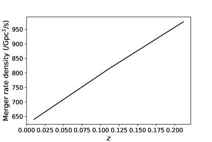
GW-Universe Toolbox is a comprehensive software package that simulates the observation on common GW sources from nHz to kHz, with various of detecting methods. We apply its ground-based detector module, where we can choose the GW detectors from a default collection of aLIGO-O3, aLIGO-design, advanced Virgo-design, KAGRA-design, Einstein Telescope and Cosmic Explorer. The targeted GW population can be chosen from binary black hole (BBH) mergers, DNS and black hole-NS mergers. With a user specified S/N threshold and observation duration, GW-Universe Toolbox will return a catalogue of simulated GW events with their physical and geometrical parameters. The uncertainties of the parameters can be also estimated based on a Fisher information matrix (FIM) based algorithm. This module is designed to be also flexible, so that users can specify their own noise curves of detectors, as well as the source population models (for details see Yi et al., 2022) For the purpose of our study, we simulate the observation with aLIGO-design, and astronomically originated GW sources from the default DNS population model (DNS-Pop I). The cosmic merger data density as function of red-shift in the DNS-Pop I model is plotted in figure 1.
2.2 modelling the background as a source population
If we lower the S/N threshold , more noise from the background of the detector will be included as signals. Thus the false-alarm rate (FAR) increases with lower . Lynch et al. (2018) found the FAR for LIGO Handford and LIGO Livingston in O1-O2 runs as function of can be fitted with an exponential function:
| (4) |
where FAR8 is the FAR when . Equation 4 is equivalent to that the accumulative frequency of the background “event” population is:
| (5) |
where is the differential number distribution of in a given observation duration , which can be obtained by taking derivative on both sides of Equation 5:
| (6) |
We want to construct a GW source population, whose accumulate merger rate distribution as function of mimics that in Equation 5. Assume the number of events from that fake population is over , we thus have:
| (7) |
Assuming is function of the binary’s masses and red-shift, we therefore have:
| (8) |
Since for DNS the mass range is small, we assume that the depends weakly on masses and attribute all the dependence of on the luminosity distance, or equivalently, on . As a result, equation 8 becomes:
| (9) |
Assume that the differential distribution of sources at the observer is:
| (10) |
and suppose the differential rate d depends on masses and separately, we obtain
| (11) |
Combining Equations (6, 9 and 10), we have
| (12) |
Integrate over mass range on both sides of Equation 12, we have
| (13) |
We know that is inversely proportional to the luminosity distance . Therefore can be represented as:
| (14) |
where is the reference luminosity distance where the of a DNS is approximately 8. Take the above relationship into Equation 13, we have:
| (15) |
In the above equation, . Work out using Equation 14 and denote
| (16) |
we rewrite Equation 15 as:
| (17) |
where the luminosity distance is denoted as function of the red-shift.
Denote the population merger rate density as function of as . The relation between and is:
| (18) |
where is the differential comoving volume of the universe. Combining Equations (17) and (18) we have the cosmic merger rate density:
| (19) |
So far, we have obtained the cosmic merger rate of the equivalent DNS population originating from the background noise. We further assume the mass dependence of is uniform over the range . Lynch et al. (2018) found that for DNS, FAR yr-1, . This provides clues for our choices of values of and , where we use yr, , Mpc, and , . We plug the above population model into the GW-Universe Toolbox, and simulate the detection of such a population of DNS with LIGO. Note that in Equation 4, is for two LIGO detectors’ combined values, but GW-Universe Toolbox simulates a single detector. So we multiply a factor to the single detector to convert it to the combined one. The number of detection as a function of is plotted in Figure 2.
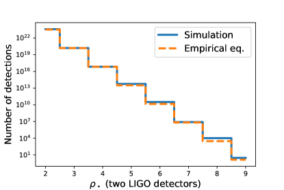
It can be seen from Figure 2 that our fake DNS population model can represent the FAR in LIGO well. Although our background population model is calibrated against the FAR function found in O1-O2, we will still employ it in this simulation study for the designed aLIGO.
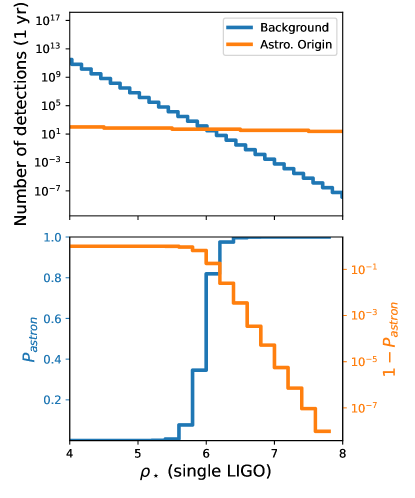
In order to compare the astronomically originated population with the background, we use the GW-Universe Toolbox to simulate a population of DNS with the default population model “Pop-A”, and the parameters for the population model are: Gpc-3/yr, Gyr, , , , , . See Yi et al. (2021) for details for the population model 111or find the description on this web-page: https://gw-universe.org/population_model.html.. In Figure 3, the upper panel shows the comparison between the numbers of sources from astronomical origin and from the background, as function of the ; in the lower panel, we show the purity () as calculated with:
| (20) |
We define as the differential purity of the marginal candidates in the neighborhood of :
| (21) |
From Figure 3, we find that at , the background events fast out-number the astronomical ones, and the purity of the detected catalogue becomes low.
2.3 The synthetic bright siren catalogues
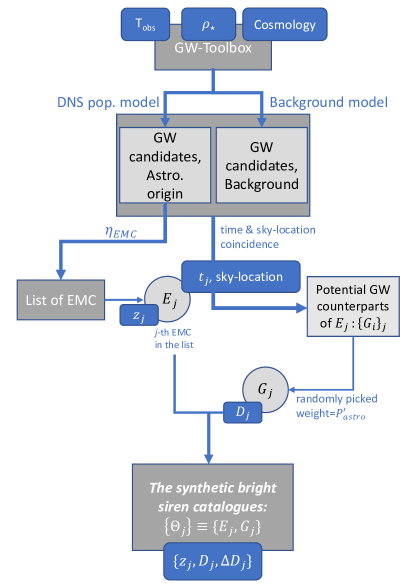
A typical GW sky localization area is a few hundreds square degrees (The LIGO Scientific Collaboration et al., 2021), and the coincident time window for a GW chirp and a typical EMC can be as large as week Abbott et al. (2017). Therefore mis-pairing between a EMC and a GW candidate is possible in the real follow-up observation campaign, when the catalogues in both bands are large. In order to include the potential mis-pairing between EMC and the GW candidates, we perform the following steps:
-
1.
Simulating a catalogue of GW candidates, which is composed of astronomical origins and background population. For each GW candidate, randomly assign their sky coordinates (, ) uniformly on the celestial sphere, and their detected time () uniformly in the observation duration.
-
2.
From the simulated astrophysical origin GW, we randomly assign a fraction of to possess detectable EMC; the redshift of each EMC is calculated based on an underlying cosmological model (Plank18 (Planck Collaboration et al., 2020) in our practice) given the simulated luminosity distance of the corresponding GW candidate.
-
3.
Up to this point, each EMC is associated with its true GW counterpart. Now we want to include the possibility of mis-pairing as in reality. For the -th EMC, we find a pool of potential GW counterparts out of the overall GW catalogue. The GW pool consists of GWs which have their and , where is the angular separation between the -th GW candidate and -th EMC, and is the uncertainty of the sky location of the -th GW; is the time lag between -th EMC and the -th GW candidate, and is the coincident time window between a GW and its possible EMC.
-
4.
From this pool, we randomly find one with a weight of , and assign it as the counterpart of the -th EMC.
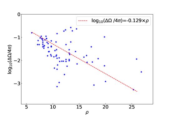
The uncertainties of sky-localization are estimated by GW-Universe Toolbox using a FIM based method. However, this estimation is based on single detector. While in reality, the localization can be much better using a network of detectors with either arriving time triangulation (Fairhurst, 2011) or phase based method (Abbott et al., 2020). For this reason, we will not use the given by the GW-Universe Toolbox, but to interpolate the empirical relationships between the and in the real observed catalogue of GWTC-3 (The LIGO Scientific Collaboration et al., 2021), using the of each GW returned from GW-Universe Toolbox. By analyzing the relationship between the sky area angle and the of the GW observed in the LIGO/Virgo O3 period, we found an empirical formula:
| (22) |
Thus, is calculated by through this formula. The relationships between the and in the real observed catalogue of GWTC-3 is shown in Figure 4.
Here we use a factor to represent the ratio between the numbers of the EMC which can be identified in the follow-up observation, and that of the total GW candidates. This , which we also refer to as the EMC follow-up efficiency, is difficult to evaluate, given its sophisticate links to EMC models, telescopes performance and multi-wavelength observation campaign (see discussion in section 5.2). In this study, we let be a free parameter, which we take two fiducial values and . The former one roughly represent the found in the current DNS catalogue so far (GW170817 and GW190425 (Abbott et al., 2020)), and the latter represents the extreme case with an optimal follow-up efficiency.
So far, we have obtained a simulated catalogue of GW and their corresponding EMC, which we refer to as the bright siren catalogue. In Figure 5 we summarize our steps of simulating the bright siren catalogue. For our purpose of cosmology model constraints, the relevant parameters of these sources are their and . The former are attributes of the GW candidates, and the latter are of those EMC. Now has a definitive value from simulation, whereas that from an observation can be shifted around this centre value according to its probability distribution. Here we assume the observed value of follows a log-normal distribution (Oguri, 2016), which is truncated at 1000 Mpc (as the detecting limit of DNS). From here on, the values of of the bright sirens are replaced by these re-sampled values according to this probability distribution.
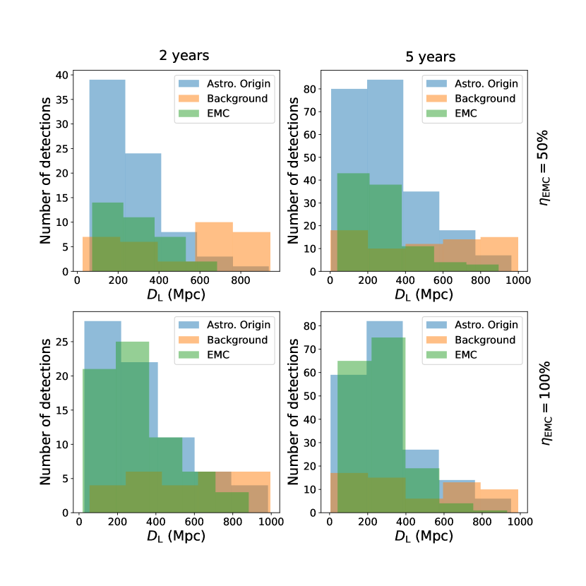
In Table 1, we list some information of the simulated catalogues with various , and . The information includes the numbers of GW candidates of astronomical and background origins, the number of EMC and that of cases of mis-pairing, in one realization of simulation. In Figure 6, we present the histogram of of GW candidates of astronomical and background origins, and those of the GW candidates associated with EMC, of different catalogues. From Figure 6 one can see that the astronomical GW candidates clearly possess a different distribution of than those of noises, indicating their different origins. While the distribution of EMC share similar shapes of those of the astronomical sources, implying that the mis-paring is rare, which is in agreement with Table 1.
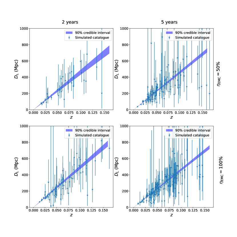
In Figure 7, we plot the vs. diagrams of the catalogues from different settings of the simulation. The blue bands are the corresponding Bayesian inferred relationship, which will be introduced in the following section.
| (years) | () | |||||
| 2 | 50 | 6 | 75 | 33 | 39 | 1 |
| 7 | 48 | 0 | 23 | 0 | ||
| 8 | 29 | 0 | 12 | 0 | ||
| 9 | 22 | 0 | 8 | 0 | ||
| 100 | 6 | 71 | 26 | 71 | 0 | |
| 7 | 37 | 0 | 37 | 0 | ||
| 8 | 28 | 0 | 28 | 0 | ||
| 9 | 20 | 0 | 20 | 0 | ||
| 5 | 50 | 6 | 225 | 69 | 114 | 7 |
| 7 | 158 | 0 | 81 | 2 | ||
| 8 | 117 | 0 | 61 | 1 | ||
| 9 | 90 | 0 | 47 | 0 | ||
| 100 | 6 | 188 | 61 | 188 | 2 | |
| 7 | 128 | 0 | 128 | 0 | ||
| 8 | 96 | 0 | 96 | 0 | ||
| 9 | 71 | 0 | 71 | 0 |
3 Bayesian inference on the from contaminated catalogues
From those generated simulated bright siren catalogues with potential contamination with fake signals and mis-identification of EMC, we use a Bayesian method to estimate cosmological parameters. By Bayes theorem, the posterior distribution of cosmological parameters is:
| (23) |
where denotes the data in the catalogue, is the likelihood of obtaining data supposing the parameters of the model is , and is the prior probability distribution of .
For the -th entry in the simulated catalogue , the likelihood is:
| (24) |
where the theoretical expected luminosity distance corresponding to red-shift , given the cosmological model parameters . is the probability of getting given the expected value from theory is ; is the probability that the real luminosity distribution is , given the observed value in the catalogue is . Both the above mentioned probability distribution are assumed to be normal in logarithm space (Oguri, 2016), with the means at and respectively, the standard deviation of , and truncated at a maximum possible horizon at Mpc.
The above integral can be approximated by the average over an ensemble of where the index runs from 1 to :
| (25) |
The ensemble is sampled from a . In our study, we take .
The likelihood for obtaining a catalogue , where , is:
| (26) |
In this work, we take as modeled by the flat -CDM cosmological model, whose parameters are , and , and . At low redshift approximation,
| (27) |
where is the speed of light.
We use a Gaussian distribution prior of , which centers at 70 km s-1 Mpc-1 with a standard deviation of 40 km s-1 Mpc-1. When considering the higher order contribution with a flat -CDM cosmology, the prior of is assumed to be uniform between 0 and 1. We use a Markov Chain-Monte Carlo (MCMC) algorithm to obtain a sample from the resulted posterior distribution with Equation 23.
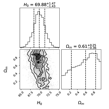
As an example, in Eigure 8 we plot the probability distributions of the priors of and respectively, and the contours (showing the 68% quantiles) of their covariance, which are inferred with an synthetic catalogue of 5 years observation, 100 and . This catalogue corresponds to the lower-right panel of Figure 7. As we can find in Figure 8, although the sub-threshold catalogue includes events as far as , the higher order effect in the relation is still not significant. As a result of this, cannot be constrained meaningfully. Therefore, in the rest of our investigation, we adopt the low red-shit approximation of as in Equation 26. Thus, the only cosmological parameter left to infer is .
4 Results and conclusion
A realization of simulated catalogue will get a posterior of . The blue region in Figure 7 represents the posterior of (90 credible interval). We get by , where is the velocity of light, is the value selected with the equal step from 0 to 0.16, is the 5 percentiles and 95 percentiles of the posterior of . Using the values of and , we plot the blue region as the 90 credible interval in Figure 7. The measurement error () is defined as half of the width of the 68 symmetric credible interval of the posterior of divided by the posterior median. The measurement bias is defined as the posterior median minus the theoretical value, which is the Plank18’s measurement result. We make many realizations of simulated catalogues with the same setting of the , and . For each realization, we calculate the measurement error and the measurement bias. After that, we obtain many and the bias of , from which we can find a 90, credible interval as the upper and lower limits as in Figure 7. We plott these region as function of for different and in Figure 9. The number of realizations we apply in this study is 30, which we find is enough to give robust upper and lower limits of the and the bias of .
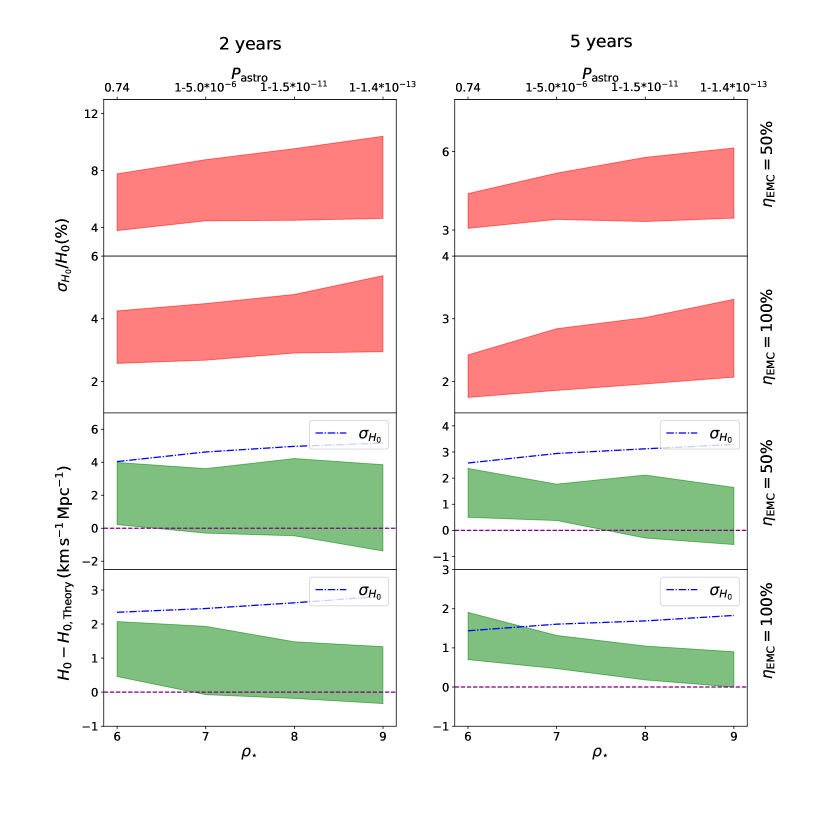
We conclude as follows:
-
•
As long as , lower the will significantly enlarge the bright-siren candidates catalogue, while the fraction of contamination due to mis-identification and background noise is small (see table 1).
-
•
The marginal candidates in the sub-threshold catalogue are those with higher red-shift and uncertainties. Inclusion of those populations will on average tighten the constraint on (upper panels of figure 9), while leaves the higher order parameters such as unconstrained.
-
•
The constraint of improves with lower , which can be seen as a general tendency in many realizations of the simulations. However, it is interesting to observe from Figure 9 that such tendency is more prominent among those realizations which result in poorest constraints.
-
•
In the lower panels of Figure 9, we can also find that, with lower , the inferred tends to bias towards greater values. We discuss on its origin in the next section.
5 discussion
5.1 A network of GW detectors
There is an obvious distinction between our simulation study and a realistic case: our simulation is for a single GW detector, while in reality GW observations are in general made by a network of detectors. This distinction has some fundamental influence on our results quantitatively. One major influence is on the sky-localization estimation, which plays a role in this study in a double-folded way: first, the mis-pairing probability is determined by the localization of candidates; second, in a standard Bayesian parameter estimation procedure, the uncertainties of the luminosity distance are in degeneration with the sky coordinates, and the former will directly enter the constraints on . The localization ability of a network of GW detectors is fundamentally different from a single detector. Since the current GW-Universe Toolbox is not able to simulate an observation with a network, and the sky coordinates uncertainties given by GW-Universe Toolbox with a FIM based on a single detector will be largely overestimated compared to a more realistic detector network, we instead use the localization estimation from the interpolation of an empirical relation between and , which is fitted from previous GW catalogues.
The ability to simulate the observation with a network is being added into the GW-Universe Toolbox as a major update. The localization of the network will be estimated with two implementations: the first one based on triangulation where only the times of arrival of the signals at all detectors are used (Fairhurst, 2011; Abbott et al., 2020); the second one also makes use of the amplitudes and phases of the signals upon arrival (Messick et al., 2017; Fairhurst, 2018).
The substitution of a single detector simulation with a network will have the following quantitative influence on our results: first, the sky coordinates uncertainties will be estimated more accurately for individual candidates, and will be in general smaller for future network than those obtained from interpolation with previous observations. The resulted mis-pairing rate will be therefore less than what is found in this simulation; the uncertainty estimation of the luminosity distance will be more accurate, where the overestimation of towards low expected in this study will be less serious. As a result, the constraints can be tighter. With the criteria of time-coincidence of signals, the background noise level is expected to be lower than that from a single detector, therefore can be even lower when the target is set to the same.
5.2 The EMC follow-up efficiency
As introduced in the above sections, well-known EMCs of DNS mergers include GRB (prompt emission and afterglow), optical and radio afterglow and kilonovae etc.. In this paper, we do not specify the EMC of GW, that is, any EMC follow-up observation campaign which leads to GW’s independent measurement will fit with our study. However, the EMC follow-up efficiency , which plays an important role in our study, does depend on the class of EMC observation targets. In this paper, we set the fiducial with 50, which roughly agrees with those of kilonovae. For a careful estimation of of a kilonova, we should take account of the variation of the efficiency with the source distance, kilonova models, filters and so on. From Sagués Carracedo et al. (2021)’s simulation of the kilonova survey, we found that kilonova models, geometry, viewing-angle, wavelength coverage, source distance and the minimum last post-merger epoch required will affect the detection probability. The kilonova models’ some parameters can be constrained by the AT 2017gfo, such as the total ejecta mass and the half-opening angle (, a lanthanide-rich component distributed within around the merger/equatorial plane (Bulla, 2019)). The limiting magnitude and distance is different for different optical telescopes. We should give a uniform maximum limiting magnitude and maximum kilonova detection distance. To simplify the problem, we can unify the wavelength coverage, i.e., the filters, and give the distribution to the viewing-angle and the minimum last post-merger epoch required. We can then simulate the kilonova follow-up efficiency, and improve our simulation of the EMC of GW.
In reality, EMC follow-up will largely depend on the multi-wavelength observation. Early information from high energy bands will largely contribute to the improvement of . In the example of GRBs, their prompt emission will be easier to be recognized, if they are simultaneous in time with GW (time lag s). In the meanwhile, they can provide the positioning information of the GW, which increases the multi-wavelength follow-up efficiency. However, the coincidence fraction between a GW and GRB prompt emission is expected to be low, due to the highly collimated emission beam of GRB prompt emission (Hendriks et al., 2022). However, if we consider the precursor and afterglow of a GRB, the coincidence fraction will increase. Similarly, they will also improve the efficiency of multi-wavelength follow-up. In addition, there is a recent model proposed in which a DNS merger involving a magnetar will have gamma-ray precursor (Zhang et al., 2022), which also is helpful to improve multi-wavelength follow-up efficiency.
5.3 Bias of the posterior
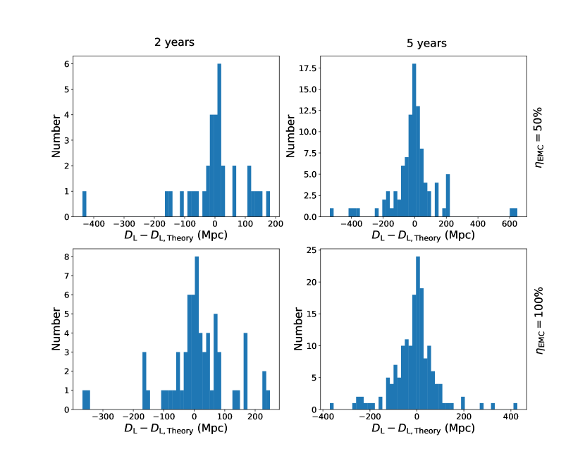
As can be seen from the lower panels of Figure 9, the inferred tends to have a higher value compared with the one which was used to generate the data. The discrepancies between the inferred ones and the injected are in most cases less than , which means the biases are not as significant as the 90% confident level. The biases are generally larger when the catalogues have smaller , or equivalently less . This tendency is partly due to the decrease of inclination towards smaller , while the absolute difference between the inferred and injected also increases. The latter is attributed to the bias of for the marginal candidates in the catalogue. As mentioned in the above section, in the calculation of the likelihood in the Bayesian inference, is re-sampled over a probability distribution of the true . The probability distribution of is assumed to be a log-normal distribution, sharply truncated at 1000 Mpc, which corresponds to the detection limit. Those marginal candidates in a sub-threshold catalogues have their close to the detection limit, and their inferred with FIM are also likely to be as large as in the same order of magnitude of . For those candidates, a re-sampling over a truncated log-normal distribution will result asymmetric and likely to have smaller values than their genuine ones. In Figure 10, we plot the histograms of the difference between the re-sampled and the corresponding genuine one, which is . We can see the asymmetry of the difference towards smaller . Such biases of of marginal candidates towards smaller values results in a posterior biases towards large values.
This finding from the simulation study may reflect a basic issue of the sub-threshold standard siren methodology: the probability distribution of will be highly asymmetrical for those marginal candidates, and thus results in biased estimation of , which will systematically towards larger values. However, we expect that with an accurate estimation of the true posterior distribution from the Bayesian method, rather than the rough methods applied here, such biases can be reduced. On the other hand, with a more realistic stimulation study, such potential bias in can be known and corrected. Such simulation studies will be crucial if the standard siren method is used to arbitrate the Hubble tension. Besides the aforementioned effect which causes the bias of in sub-threshold catalogues, there are two other sources of biases, which will inflate the inferred value as discussed in literature. One originates from a combination effect of the inclination-distance degeneracy and the selection favorite over small inclination angle (Gerardi et al., 2021); the other effect is due to the selection bias of the EMC towards small inclination angle (Chen, 2020). Both effects will result in a skewed luminosity distance posterior, and thus bias the . Gagnon-Hartman et al. (2023) provided a method which can correct the biases from the above-mentioned two effects. In our study, these two effects do not contribute to the bias, since we use a presumed posterior. As discussed above, the source of bias is a separated one, arising from the events near the detection horizon. It therefore becomes dominating in the case of using sub-threshold catalogue, where the number of events near the horizon is large.
Acknowledgments
This work is supported by the National Key R&D Program of China (2021YFA0718500). SXY acknowledges the support by the Institute of High Energy Physics (Grant No. E25155U1).
References
- Abbott et al. (2017) Abbott, B. P., Abbott, R., Abbott, T. D., et al. 2017, Nature, 551, 85. doi:10.1038/nature24471
- Abbott et al. (2017) Abbott, B. P., Abbott, R., Abbott, T. D., et al. 2017, ApJ, 848, L12. doi:10.3847/2041-8213/aa91c9
- Abbott et al. (2020) Abbott, B. P., Abbott, R., Abbott, T. D., et al. 2020, ApJ, 892, L3. doi:10.3847/2041-8213/ab75f5
- Abbott et al. (2020) Abbott, B. P., Abbott, R., Abbott, T. D., et al. 2020, Living Reviews in Relativity, 23, 3. doi:10.1007/s41114-020-00026-9
- Bulla (2019) Bulla, M. 2019, MNRAS, 489, 5037. doi:10.1093/mnras/stz2495
- Chase et al. (2022) Chase, E. A., O’Connor, B., Fryer, C. L., et al. 2022, ApJ, 927, 163. doi:10.3847/1538-4357/ac3d25
- Chen et al. (2018) Chen, H.-Y., Fishbach, M., & Holz, D. E. 2018, Nature, 562, 545. doi:10.1038/s41586-018-0606-0
- Chen (2020) Chen, H.-Y. 2020, Phys. Rev. Lett., 125, 201301. doi:10.1103/PhysRevLett.125.201301
- Del Pozzo (2012) Del Pozzo, W. 2012, Phys. Rev. D, 86, 043011. doi:10.1103/PhysRevD.86.043011
- Fairhurst (2011) Fairhurst, S. 2011, Classical and Quantum Gravity, 28, 105021. doi:10.1088/0264-9381/28/10/105021
- Fairhurst (2018) Fairhurst, S. 2018, Classical and Quantum Gravity, 35, 105002. doi:10.1088/1361-6382/aab675
- Feeney et al. (2021) Feeney, S. M., Peiris, H. V., Nissanke, S. M., et al. 2021, Phys. Rev. Lett., 126, 171102. doi:10.1103/PhysRevLett.126.171102
- Fishbach et al. (2019) Fishbach, M., Gray, R., Magaña Hernandez, I., et al. 2019, ApJ, 871, L13. doi:10.3847/2041-8213/aaf96e
- Gagnon-Hartman et al. (2023) Gagnon-Hartman, S., Ruan, J., & Haggard, D. 2023, MNRAS, 520, 1. doi:10.1093/mnras/stad069
- Gerardi et al. (2021) Gerardi, F., Feeney, S. M., & Alsing, J. 2021, Phys. Rev. D, 104, 083531. doi:10.1103/PhysRevD.104.083531
- Ghosh et al. (2022) Ghosh, T., Biswas, B., & Bose, S. 2022, arXiv:2203.11756
- Hendriks et al. (2022) Hendriks, K., Yi, S.-X., & Nelemans, G. 2022, arXiv:2208.14156
- Hinshaw et al. (2013) Hinshaw, G., Larson, D., Komatsu, E., et al. 2013, ApJS, 208, 19. doi:10.1088/0067-0049/208/2/19
- Holz & Hughes (2005) Holz, D. E. & Hughes, S. A. 2005, ApJ, 629, 15. doi:10.1086/431341
- Jang & Lee (2017) Jang, I. S. & Lee, M. G. 2017, arXiv:1702.01118
- Lynch et al. (2018) Lynch, R., Coughlin, M., Vitale, S., et al. 2018, ApJ, 861, L24. doi:10.3847/2041-8213/aacf9f
- MacLeod & Hogan (2008) MacLeod, C. L. & Hogan, C. J. 2008, Phys. Rev. D, 77, 043512. doi:10.1103/PhysRevD.77.043512
- Messick et al. (2017) Messick, C., Blackburn, K., Brady, P., et al. 2017, Phys. Rev. D, 95, 042001. doi:10.1103/PhysRevD.95.042001
- Metzger et al. (2010) Metzger, B. D., Martínez-Pinedo, G., Darbha, S., et al. 2010, MNRAS, 406, 2650. doi:10.1111/j.1365-2966.2010.16864.x
- Mortlock et al. (2019) Mortlock, D. J., Feeney, S. M., Peiris, H. V., et al. 2019, Phys. Rev. D, 100, 103523. doi:10.1103/PhysRevD.100.103523
- Nissanke et al. (2010) Nissanke, S., Holz, D. E., Hughes, S. A., et al. 2010, ApJ, 725, 496. doi:10.1088/0004-637X/725/1/496
- Oguri (2016) Oguri, M. 2016, Phys. Rev. D, 93, 083511. doi:10.1103/PhysRevD.93.083511
- Phillips (1993) Phillips, M. M. 1993, ApJ, 413, L105. doi:10.1086/186970
- Planck Collaboration et al. (2014) Planck Collaboration, Ade, P. A. R., Aghanim, N., et al. 2014, A&A, 571, A16. doi:10.1051/0004-6361/201321591
- Planck Collaboration et al. (2016) Planck Collaboration, Ade, P. A. R., Aghanim, N., et al. 2016, A&A, 594, A13. doi:10.1051/0004-6361/201525830
- Planck Collaboration et al. (2020) Planck Collaboration, Aghanim, N., Akrami, Y., et al. 2020, A&A, 641, A6. doi:10.1051/0004-6361/201833910
- Rastinejad et al. (2022) Rastinejad, J. C., Paterson, K., Fong, W., et al. 2022, ApJ, 927, 50. doi:10.3847/1538-4357/ac4d34
- Riess et al. (1995) Riess, A. G., Press, W. H., & Kirshner, R. P. 1995, ApJ, 438, L17. doi:10.1086/187704
- Riess et al. (2016) Riess, A. G., Macri, L. M., Hoffmann, S. L., et al. 2016, ApJ, 826, 56. doi:10.3847/0004-637X/826/1/56
- Riess et al. (2022) Riess, A. G., Yuan, W., Macri, L. M., et al. 2022, ApJ, 934, L7. doi:10.3847/2041-8213/ac5c5b
- Sagués Carracedo et al. (2021) Sagués Carracedo, A., Bulla, M., Feindt, U., et al. 2021, MNRAS, 504, 1294. doi:10.1093/mnras/stab872
- Schutz (1986) Schutz, B. F. 1986, Nature, 323, 310. doi:10.1038/323310a0
- Spergel et al. (2007) Spergel, D. N., Bean, R., Doré, O., et al. 2007, ApJS, 170, 377. doi:10.1086/513700
- The LIGO Scientific Collaboration et al. (2021) The LIGO Scientific Collaboration, the Virgo Collaboration, the KAGRA Collaboration, et al. 2021, arXiv:2111.03606
- Verde et al. (2019) Verde, L., Treu, T., & Riess, A. G. 2019, Nature Astronomy, 3, 891. doi:10.1038/s41550-019-0902-0
- Wang et al. (2003) Wang, L., Goldhaber, G., Aldering, G., et al. 2003, ApJ, 590, 944. doi:10.1086/375020
- Xiao et al. (2022) Xiao, S., Zhang, Y.-Q., Zhu, Z.-P., et al. 2022, arXiv:2205.02186
- Yi et al. (2021) Yi, S.-X., Nelemans, G., Brinkerink, C., et al. 2021, arXiv:2106.13662
- Yi et al. (2022) Yi, S.-X., Nelemans, G., Brinkerink, C., et al. 2022, A&A, 663, A155. doi:10.1051/0004-6361/202141634
- Zhang et al. (2022) Zhang, Z., Yi, S.-X., Zhang, S.-N., et al. 2022, ApJ, 939, L25. doi:10.3847/2041-8213/ac9b55