High gradient twin $e^{+}e^{-}$, $e^{-}e^{-}$ linear colliders with energy recovery.

Abstract

Recently, a high energy superconducting (SC) $e^{+}e^{-}$ linear collider (LC) with energy recovery (ERLC) have been proposed where twin RF structures are used to avoid parasitic collisions within linacs. Such a collider can operate in a duty cycle (DC) or in a continuous (CW) modes (if sufficient power) with a luminosity of ${\cal O}(10^{36})$ ${\rm\,cm}^{-2}{\rm s}^{-1}$ at $2E_{0}=250-500$ GeV. In this paper, I note that the luminosity at the ERLC operating in duty cycle mode does not depend on the accelerating gradient (at the same total power), but only slightly changes as $L\propto\sqrt{Q}$. So, the ERLC can work at maximum available acceleration gradients. The article also considers the $e^{-}e^{-}$ twin collider with energy recovery and estimates the achievable luminosity. Such an $e^{-}e^{-}$ collider is much simpler than $e^{+}e^{-}$ one, because beam recirculation is not required, can have $L$ well above $10^{36}$ cm^-2s^-1. It also has a fairly rich physics program.

1 Introduction

Linear $e^{+}e^{-}$ colliders (LC) have been actively developed since the 1970s as a way to reach higher energies. There were many LC projects in the 1990s (VLEPP, NLC, JLC, CLIC, TESLA, etc.); since 2004 only two remain: ILC [1, 2] and CLIC [3]. The ILC is based on superconducting (SC) Nb technology (in the footsteps of the TESLA), while the CLIC uses Cu cavities and operates at room temperature. Both colliders operate in a pulsed mode, beams after the collision are sent to the beamdump. The ILC is ready for construction, but there is no decision already many years due to uncertainty in the choice of the next collider after the results from the LHC. At the same time, new ideas are emerging on how to improve linear colliders, reduce size and cost, or increase luminosity. Recent review of all approaches, prepared for Snowmass-2021, in given in ref. [4].

In this short article, I continue the discussion of my recent proposal of the twin superconducting $e^{+}e^{-}$ linear collider with energy recovery (ERLC) [5], its scheme is shown see Fig. 1. In this collider, the beams are accelerated and then decelerated in separate parallel linacs with coupled RF systems, so there are no parasitic collisions (which would destroy the beams). The same e⁺ and e^- beams are used many times (>$10^{5}$), so all the advantages of superconducting technology are used. The attainable $e^{+}e^{-}$ luminosity ${\cal O}(10^{36})$ ${\rm\,cm}^{-2}{\rm s}^{-1}$ is much higher than with a single pass ILC. In my previous publication [5], the rather low accelerating gradient, $G=20$ MeV/m, was assumed, at which the quality factor of the SC cavities $Q$ is close to the maximum. It looks like a disadvantage, because for ILC, an accelerating gradient of $G\approx 35$ MeV/m is planned. Moreover, it was recently noticed that it is possible to almost double the gradient if instead of a standing wave (SW) a traveling wave (TW) is used  [6]. In this case, gradients of 70 (Nd)–100 (Nb₃Sn) MeV/m are possible, although the Nb₃Sn technology is not ready yet.

In this article, I want to draw your attention to the fact that ERLC collider can also work at high gradients, and the luminosity does not depend on the accelerating gradient (at the same total power), but only slightly changes due to the dependence of the quality factor on the gradient: $L\propto\sqrt{Q}$. Also, the case of $e^{-}e^{-}$ ERLC is considered. Such an $e^{-}e^{-}$ collider is much simpler than $e^{+}e^{-}$, because beam recirculation is not required, and the luminosity higher than in $e^{-}e^{-}$ collisons can be reached.

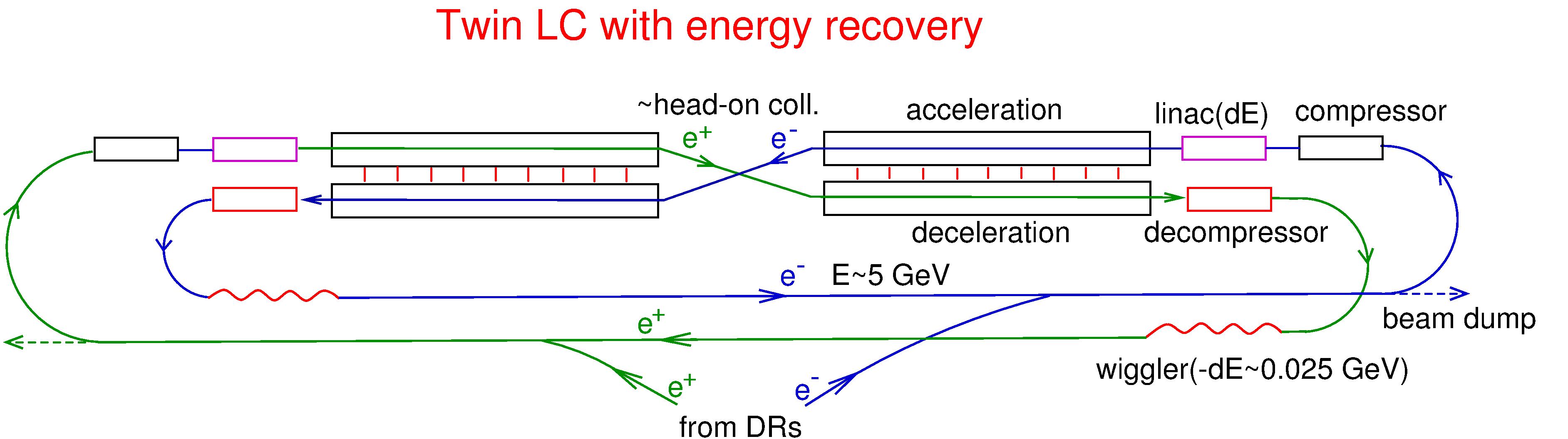
Figure 1: The layout of the SC twin $e^{+}e^{-}$ linear collider.

2 $e^{+}e^{-}$ ERLC: dependence of the luminosity on G and Q

Here we simply follow the ref. [5], where the necessary formula was obtained and the dependence on $Q$ was emphasized, but the dependence on the accelerating gradient was not mentioned directly.

We assume the case of operation with a duty cycle (DC), when the collider works part of time, $DC<1$. This mode can be implemented at any available average power, and it is only possible at high acceleration gradients. Let us find the optimum number of particles in one bunch $N$ when the luminosity is maximum for a given power consumption.

There are two main energy consumers

• Electric power for cooling of the RF losses in cavities at low temperatures, it does not depend on the number of particles in the bunch.

• Electric power for compensation and removal of High Order Mode (HOM) losses. The HOM energy loss by the bunch per unit length is proportional to $N^{2}$. If the distance between bunches $d$, then for the given collider $P_{\rm HOM}\propto N^{2}/d$.

The total power (only main contributions)

$$P_{tot}=\left(k_{1}+k_{2}\frac{N^{2}}{d}\right)\times DC,$$ (2.1)

where coefficients $k_{1}$ and $k_{2}$ (’$a$’ and ’$b$’ in [5]) describe RF and HOM losses, respectively, they are both proportional to the collider length (or $E_{0}$).

The $e^{+}e^{-}$ luminosity in one bunch collision $L_{1}$ is determined by collision effects (beamstrahlung, bunch instability). For flat beams, these effects are the same when $N$ varies proportional to the horizontal beam size $\sigma_{x}$, so $L_{1}\propto N$ and the total luminosity

$$L\propto\frac{N}{d}DC=\frac{N}{d}\left(\frac{P}{k_{1}+k_{2}N^{2}/d}\right).$$ (2.2)

The maximum luminosity $L$

$$L\propto\frac{P}{\sqrt{k_{1}k_{2}d}}\;\;\;\;{\rm at}\;\;\;\;N=\sqrt{\frac{k_{1}d}{k_{2}}},\;\;\;\;DC=\frac{P}{2k_{1}}.$$ (2.3)

The luminosity reaches the maximum when the energy spent for removal of $RF$ and $HOM$ losses are equal. We see from (2.3) that for the fixed total power

1. $L\propto 1/\sqrt{d}$, so the distance between bunches $d$ should be as small as possible ($d=\lambda_{\rm RF}$ is the best);

2. $L\propto\sqrt{Q}$, because $k_{1}\propto 1/Q$;

3. $L$ does not depend on the acceleration gradient $G$. This is because the collider length $l_{c}\propto 1/G$, so $k_{2}\propto 1/G$, and the RF losses $k_{1}\propto G^{2}\times l_{c}\propto G$, as result $L=\rm const$;

4. the optimal $N=\sqrt{k_{1}d/k_{2}}\propto G\sqrt{d/Q}$, $DC\propto 1/G$

We see, that the path to a high ERLC accelerating gradient is open. The luminosity does not depend on $G$ and depends weakly on $Q$. This unexpected dependence is due to optimal change of $N$ and $DC$. At $G=20$ MeV/m the optimum is $N\sim 10^{9}$ [5], so there is no problem to increase it several times for higher gradients, such values of $N$ are typical for linear colliders.

3 $e^{-}e^{-}$ ERLC

Let us consider a twin $e^{-}e^{-}$ linear collider with energy recovery. Such a collider is also of a great interest, its physics program was discussed at several dedicated workshops [7, 8, 9], and this option is always taken into account considering LC projects. A principle scheme of such $e^{-}e^{-}$ collider is shown in Fig. 2.

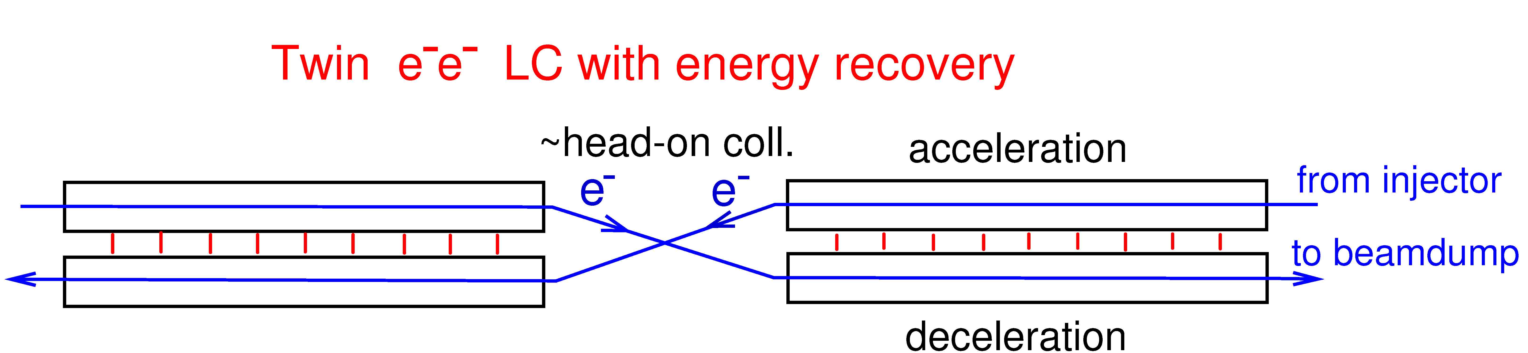
Figure 2: The layout of the SC twin $e^{-}e^{-}$ linear collider.

It is much simpler than the $e^{+}e^{-}$ collider because no beam recirculation is required, electron beams with small emittances can be prepared anew each time. Beams can be more tightly focussed than in $e^{+}e^{-}$ case since the beams are used only once. The difference from the ILC that in the ERLC-$e^{-}e^{-}$ beams after collision return their energy to the RF field of the collider. Not completely, part of its energy is lost due to beamstrahlung at the interaction point (IP) and must be compensated by the RF-system without energy recovery. For the $e^{+}e^{-}$ case such average energy losses are not important. This requires additional electricity. In addition to average energy losses, there is also a fairly wide beam energy spread with tails. To make full use of the beam energy, a beam decompressor can be installed at the end of the linac in order to reduce the energy spread, or several mini-beamdumps can be arranged to remove the tails of the energy particles with lowest energy. For further consideration, we will simply assume that it is necessary compensate for twice the average energy loss, and it is done with some efficiency $\varepsilon_{\rm rf}\sim 50$ %. Let’s repeat a similar considerations, as it was done above for $e^{+}e^{-}$, but taking into account an additional source of energy consumption: beamstrahlung at the IP.

The relative energy loss due to beamstrahlung [10]

$$\delta=\frac{\Delta E}{E_{0}}\approx\frac{0.84r_{e}^{3}N^{2}\gamma}{\sigma_{z}\sigma_{x}^{2}},$$ (3.1)

where $r_{e}=e^{2}/mc^{2}$. The power required for compensation of these energy losses for two beams, multiplied by a factor of two, as mentioned above, is

$$P_{rad}=\frac{4NcE_{0}\delta}{\varepsilon_{\rm rf}d}=k_{3}\frac{N^{3}}{\sigma_{z}\sigma_{x}^{2}d},\,\,\,\,\,\,\,k_{3}=\frac{3.35E_{0}r_{e}^{3}\gamma c}{\varepsilon_{\rm rf}}.$$ (3.2)

Similar to (2.1), total power now has three main contributions

$$P_{tot}=\left(k_{1}+k_{2}\frac{N^{2}}{d}+k_{3}\frac{N^{3}}{\sigma_{z}\sigma_{x}^{2}d}\right)\times DC.$$ (3.3)

The luminosity

$$L\approx\frac{N^{2}cH_{D}}{4\pi\sigma_{x}\sigma_{y}d}\times DC,$$ (3.4)

where the vertical beam size $\sigma_{y}\approx\sqrt{\varepsilon_{ny}\sigma_{z}/\gamma}$, $H_{D}\sim 0.8$ - a geometric factor. Substituting (3.3) to (3.4) we have

$$L=k_{0}\frac{N^{2}}{\sigma_{x}\sigma_{z}^{1/2}}\frac{P}{\left(k_{1}d+k_{2}N^{2}+k_{3}N^{3}/\sigma_{z}\sigma_{x}^{2}\right)},\,\,\,\,k_{0}=\frac{c\gamma^{1/2}H_{D}}{4\pi\varepsilon_{ny}^{1/2}}.$$ (3.5)

The luminosity depends on two parameters: $N$ and $y=\sigma_{x}\sigma_{z}^{1/2}$

$$L\propto\frac{N^{2}}{y\left(k_{1}d+k_{2}N^{2}+k_{3}N^{3}/y^{2}\right)}.$$ (3.6)

For fixed $N$ the maximum luminosity is reached at

$$y^{2}=\frac{N^{3}k_{3}}{k_{1}d+k_{2}N^{2}}.$$ (3.7)

At this value, the power consumption for compensation of radiation losses is 1/2 of the total power. Substituting (3.7) to (3.6) we get

$$L^{2}\propto\frac{NP^{2}}{k_{1}d+k_{2}N^{2}}.$$ (3.8)

This dependance $L^{2}$ on $N$ is the same as for $L$ in the $e^{+}e^{-}$ case (2.2). The maximum luminosity is reached at the same value of $N$ as in the $e^{+}e^{-}$ case.

$$N=\sqrt{k_{1}d/k_{2}}.$$ (3.9)

This means that under optimal conditions $P_{\rm RF}=P_{\rm HOM}=0.5P_{rad}=0.25P$. The corresponding value of the optimal duty cycle

$$DC=P/4k_{1},$$ (3.10)

that is two times less than in the $e^{+}e^{-}$ case. Substituting all to (3.4) we obtain the maximum luminosity

$$L=0.022\frac{(c\varepsilon_{\rm rf})^{1/2}H_{D}P}{\varepsilon_{ny}^{1/2}(k_{1}k_{2}d)^{1/4}E_{0}^{1/2}r_{e}^{3/2}}.$$ (3.11)

Beside the beam energy losses, considered above, there is another important collision effect due to beam repulsion. It is determined by the disruption parameter [10]

$$D_{y}=\frac{2Nr_{e}\sigma_{z}}{\gamma\sigma_{x}\sigma_{y}}.$$ (3.12)

For $e^{-}e^{-}$ collisions the optimal (maximum) value for $D_{y}\approx 5$ [11]. It does not affect the luminosity calculated above, but it determines the bunch length. Indeed, above we found optimal values of $N$ and $\sigma_{x}\sigma_{z}^{1/2}$. Substitution to (3.12) gives the maximum value of $\sigma_{z}$.

From (3.11) we see that $e^{-}e^{-}$ luminosity depends very weakly on SC linac properties, as $L\propto 1/(k_{1}k_{2}d)^{1/4}$ (in $e^{+}e^{-}$ case it was $L\propto 1/(k_{1}k_{2}d)^{1/2}$. Similar to $e^{+}e^{-}$ the luminosity does not depend on the accelerating gradient, the dependence on the quality factor is even weaker: $L\propto Q^{1/4}$. The $e^{-}e^{-}$ luminosity $L\propto P/E_{0}$, as soon as $k_{1}$ and $k_{2}$ are proportional to the energy.

Let’s move on to luminosity estimates, using number for $k_{1}$ and $k_{2}$ from ref. [5]. For Nd ILC-like cavities with $f_{\rm rf}=1.3$ GHz $k_{1}\approx 305$ MW, $k_{2}\approx(240\,{\rm MW}/10^{18})\times 23{\rm cm}$. For Nb₃Sn cavities the value of $k_{1}$ is 4 times smaller due to higher cryogenic efficiency. In the case of BCS surface conductivity $k_{1}\propto f_{\rm rf}$, $k_{2}\propto f_{\rm rf}^{2}$, $d\propto 1/f_{\rm rf}$. Possible parameters for two case are given in Table 1 for $2E_{0}=250$ GeV with $G=20$ MeV/m. For other cases numbers can be recalculated easily.

Table 1: Parameters of $e^{-}e^{-}$ ERLC, $2E_{0}=250$ GeV.

		Nb,1.8K	$\rm Nb_{3}Sn,4.5K$
		1.3 GHz	0.65 GHz
Energy $2E_{0}$	GeV	250	250
Luminosity ${\mathcal{L}}_{{\rm tot}}$	$10^{36}$${\rm\,cm}^{-2}{\rm s}^{-1}$	2	4
$P$ (wall) (collider)	MW	100	100
Duty cycle, $DC$		0.082	0.65
Accel. gradient, $G$	MV/m	20	20
$N$ per bunch	$10^{9}$	1.13	1.13
Bunch distance	m	0.23	0.46
$\varepsilon_{x,\,n}$/$\varepsilon_{y,\,n}$	$10^{-6}$ m	1/0.02	1/0.02
$\beta^{*}_{x}$/$\beta_{y}$ at IP	cm	0.67/0.008	1.33/0.017
$\sigma_{x}$ at IP	${\,\mu\rm m}$	0.165	0.23
$\sigma_{y}$ at IP	nm	2.6	3.65
$\sigma_{z}$ at IP	cm	0.008	0.017

4 Conclusion

Twin $e^{+}e^{-}$ and $e^{-}e^{-}$ linear colliders with the energy recovery open the way to very high luminosities. This article shows that the luminosity of the ERLC collider operating in duty cycle mode does not depend on the accelerating gradient and only weakly depends on quality factor of accelerating cavities: $L_{e^{+}e^{-}}\propto Q^{1/2}$, $L_{e^{-}e^{-}}\propto Q^{1/4}$. Previously [5], $e^{+}e^{-}$ ERLC with repeated use of bunches was considered; in this article, the case of $e^{-}e^{-}$ ERLC with single use of electron bunches is considered for the first time. Its luminosity at P= 100 MW for two considered cases is (2–4)$\times 10^{36}$ ${\rm\,cm}^{-2}{\rm s}^{-1}$, which is 3–6 times higher than the $e^{+}e^{-}$ luminosity for similar SC technologies. Energy recovery superconducting accelerators have many possible applications [12], so one can hope for rapid progress in this area.

This work was supported by RFBR-DFG Grant No 20-52-12056.

References

- [1] T. Behnke et al., “The Intern. Linear Collider Technical Design Report - Volume 1: Executive Summary,” arXiv:1306.6327 [physics.acc-ph].
- [2] P. Bambade et al., “The Intern. Lin. Collider: A Global Project”, arXiv:1903.01629 [hep-ex] (2019).
- [3] M. Aicheler et al., “A Multi-TeV Linear Collider Based on CLIC Technology: CLIC Conceptual Design Report,” CERN-2012-007. doi:10.5170/CERN-2012-007.
- [4] A. Faus-Golfe, G. H. Hoffstaetter, Q. Qin, F. Zimmermann, T. Barklow, E. Barzi, S. Belomestnykh, M. Biagini, M. C. Llatas and J. Gao, et al. Accelerators for Electroweak Physics and Higgs Boson Studies, arXiv:2209.05827.
- [5] V. I. Telnov, A high-luminosity superconducting twin e+e- linear collider with energy recovery, JINST 16 (2021) no.12, P12025, arXiv:2105.11015.
- [6] S. Belomestnykh, P. C. Bhat, A. Grassellino, M. Checchin, D. Denisov, R. L. Geng, S. Jindariani, M. Liepe, M. Martinello and P. Merkel, et al. Higgs-Energy LEptoN (HELEN) Collider based on advanced superconducting radio frequency technology, arXiv:2203.08211.
- [7] C. A. Heusch, Electron electron linear collider. Proceedings, 2nd Workshop, e-e-’1997, Santa Cruz, USA, September 22-24, 1997, Int. J. Mod. Phys. A 13 (1998), pp.2217-2549.
- [8] C. A. Heusch, Electron electron linear collider. Proceedings, 3rd Workshop, e- e- 1999, Santa Cruz, USA, December 10-12, 1999, Int. J. Mod. Phys. A 15 (2000), pp.2347-2628.
- [9] C. Heusch, Electron electron collisions at TeV energies. Proceedings, 4th Workshop, e-e-’01, Santa Cruz, USA, December 7-9, 2001, Int. J. Mod. Phys. A 18 (2003), pp.2733-2926.
- [10] K. Yokoya and P. Chen, “Beam-beam phenomena in linear colliders,” Lect. Notes Phys. 400 (1992), 415-445.
- [11] K. A. Thompson, Optimization of NLC luminosity for e-e-running, Int. J. Mod. Phys. A 15 (2000), 2485-2493 SLAC-PUB-8715.
- [12] C. Adolphsen, K. Andre, D. Angal-Kalinin, M. Arnold, K. Aulenbacher, S. Benson, J. Bernauer, A. Bogacz, M. Boonekamp and R. Brinkmann, et al. The Development of Energy-Recovery Linacs, arXiv:2207.02095.