Identification-robust inference for the LATE with
high-dimensional covariates

Abstract

This paper presents an inference method for the local average treatment effect (LATE) in the presence of high-dimensional covariates, irrespective of the strength of identification. We propose a novel high-dimensional conditional test statistic with uniformly correct asymptotic size. We provide an easy-to-implement algorithm to infer the high-dimensional LATE by inverting our test statistic and employing the double/debiased machine learning method. Simulations indicate that our test is robust against both weak identification and high dimensionality concerning size control and power performance, outperforming other conventional tests. Applying the proposed method to railroad and population data to study the effect of railroad access on urban population growth, we observe that our methodology yields confidence intervals that are 49% to 92% shorter than conventional results, depending on specifications.
Keywords: Weak identification, local average treatment effect, double/debiased machine learning, high-dimensional covariates.

1 Introduction

We propose a high-dimensional conditional test statistic with uniformly correct asymptotic size. The proposed method exhibits robustness against weak identification and high dimensionality in the LATE framework. Furthermore, we provide a practical guideline, including a step-by-step algorithm, for drawing inferences for the LATE with high-dimensional controls. This algorithm entails (1) inverting the proposed statistics to derive confidence intervals and (2) applying machine-learning approaches to overcome the regularization bias and overfitting within the high-dimensional model. The objective is motivated by the persistent challenges of the weak-instrument problem in empirical research and the prevalence of rich data in the contemporary big data era.

In models where certain explanatory variables correlate with the error term, least squares estimators yield inconsistent coefficient estimates. To address this, instrumental variables (IV) are often employed, as they are uncorrelated with the error term but correlated with the endogenous explanatory variables. Nonetheless, if the correlation between the instruments and endogenous variables is weak, IV estimation becomes imprecise, resulting in unreliable tests and confidence intervals. This presents the weak-instrument problem, a notable concern in empirical practice.

Empirical researchers often aim to make inferences about the coefficients of endogenous variables in IV regression. An example is the influential study by Angrist and Krueger (1991), using quarter of birth as an IV to estimate returns from schooling. However, Bound et al. (1995) argue that Angrist and Krueger’s results may be unreliable due to the weak correlation between one’s quarter of birth and their education attainment. Moreover, the common practice of pretesting, with a rule-of-thumb F-statistic threshold of 10 proposed by Staiger and Stock (1997), is challenged by Lee et al. (2022). In their paper, they introduce a novel critical value function and reveal that achieving a true 5 percent test with critical value of 1.96 instead requires an F exceeding 104.7. Applying this criterion to their sample of 61 American Economic Review papers published between 2013 and 2019, they find that a quarter of the specifications initially presumed to be statistically significant are, in fact, insignificant.

Angrist and Imbens (1995a) introduce a framework for estimating the local average treatment effect (LATE). This estimate captures the treatment effect for a group of compliers who decide to take the treatment if and only if assigned to the treatment group, but not if assigned to the control group. Employing the IV method to estimate LATE has garnered considerable attention in the literature. Within the LATE framework, weak identification emerges either when instruments correlate weakly with endogenous regressors or when the proportion of compliers is relatively small. We are particularly interested in exploring and addressing this weak identification issue within the LATE framework for several reasons. On the one hand, while compliers might be a minority, they often represent the population of critical interest to policymakers. Take the Vietnam-era draft lottery in Angrist (1990) as an example. Even though compliers constituted a minority, approximately 0.10 to 016, their experiences provide valuable insights into the draft’s direct consequences for individuals at the decision-making margin, thereby shedding light on the immediate effects of veteran status on civilian earnings. On the other hand, natural experiments often present challenges of weak identification, especially when researchers have no control over the size of the complier group, as highlighted by the instrument strength concerns in Angrist and Krueger (1991). Our objective is to yield reliable outcomes in situations where interventions first impact only a small group, both theoretically and practically. Understanding this impact is crucial for expanding or scaling such interventions.

The issue of weak instruments has been rigorously explored in the literature, leading to the development of diverse econometric techniques to estimate and infer about a structural parameter $\theta$ based on moment equailities. Specifically, many models suggest that certain functions of the data and model parameters possess a mean of zero when evalueted at the true parameter value $\theta_{0}$. Our research primarily concentrates on testing the hypothesis that this mean function is indeed zero at $\theta_{0}$, which is the true LATE value. The existing literature proposes numerous tests for this hypothesis, as demonstrated by works such as Stock and Wright (2000), Kleibergen (2002), and Andrews and Mikusheva (2016). While these studies present methods tailored for inference about target parameters in the presence of weak identification, they overlook models equipped with high-dimensional covariates. However, these models are becoming increasingly prevalent in today’s big-data environment. On the one hand, accounting for a large number of covariates can bolster the validity of the IV within the LATE framework. On the other hand, established identification-robust methods encounter challenges in the presence of many covariates, particularly experiencing severe size distortions in high-dimensional covariates scenarios. Our contribution generalizes prior research by developing an identification-robust method that employs machine-learning techniques, enabling us to explore a broader set of controls than previously explored.

Based on our simulation results, our proposed method outperforms the conventional identification-robust method. For comparison, we selected the conditional quasi-likelihood ratio test introduced by Andrews and Mikusheva (2016) as the representative conventional identification-robust test. Our findings demonstrate that within the high-dimensional LATE framework, especially when the dimensionality of covariates is comparable to the sample size, our method consistently maintains correct size control and demonstrates good power performance. Conversely, the traditional approach experiences severe size distortion, both in strongly identified cases (where the share of compliers is 0.5) and in weakly identified scenarios (where the share of compliers is 0.1). This discrepancy arises because the conventional identification-robust approach lacks a feature selection stage. Instead, it incorporates all covariates, leading to potential overfitting issues. In contrast, our proposed method employs machine-learning techniques for model selection.

Similarly, our proposed method also surpasses existing machine-learning approaches. Here, we select two machine-learning methods: one proposed by Chernozhukov et al. (2018a) and the other by Belloni et al. (2017). While these conventional machine-learning techniques demonstrate robustness in high-dimensional contexts, they underperform, showing significant size distortion and power reduction in weak identification scenarios. This shortcoming arises because they construct confidence intervals based on the normal distribution rather than employing the test inversion of an identification-robust test statistic. Overall, our proposed method consistently exhibits robustness to both weak identification and high dimensionality in terms of size control and power performance. We highlight that our test maintains uniform size control across a broad range of data-generating processes, accommodating both low and high-dimensional scenarios, as well as weakly and strongly identified cases.

In our empirical studies, we employ our proposed method to re-examine two IV estimations. The first is by Hornung (2015) that investigates the effect of railroad access on city population growth in the 19th-century Prussia. The second is by Ambrus et al. (2020), which explores the long-term impact of cholera-related deaths on rental prices in a neighborhood of 19th-century London. For the first application, depending on various specifications, the dataset includes approximately 900 observations and 200 covariates. Our analysis reveals that our proposed method produces narrower confidence intervals, in comparison to the conventional identification-robust test and existing machine-learning methods used in our simulation study. The shorter confidence intervals indicate the efficiency of our proposed method, which stems from addressing both the weak identification issue and the inclusion of high-dimensional covariates to mitigate unobserved confoundedness. Moreover, coefficients that are initially significant with the conventional identification-robust method often become insignificant when our method is applied. The second study yields similar results, further underscoring the robustness and consistency of our approach.

This paper advances the well-established literature on weak identification by providing procedures for inference and the construction of confidence intervals for the LATE parameters in high-dimensional models. To the best of our knowledge, this is the first paper to draw inferences about the high- dimensional LATE model, irrespective of identification strength. We develop a high-dimensional conditional test statistic with uniformly correct asymptotic size. Furthermore, we provide a practical guideline, complete with a step-by-step algorithm, for drawing inferences and determining confidence intervals for the high-dimensional LATE using machine-learning methods, specifically based on the lasso technique.

1.1 Relations to the Literature

This paper contributes to the literature on weak identification and high-dimensional models by providing a test tailored for making inferences regarding the LATE in the presence of high-dimensional covariates.

Since the 1990s, weak identification in the IV context has received considerable attention in the literature. Staiger and Stock (1997) conceptualized the coefficients on the instruments in the first-stage equation as residing in a $N^{-1/2}$ vicinity of zero, aptly naming this the “local-to-zero” weakly correlated case. To test if the mean function equals to zero at the true parameter value $\theta_{0}$, Stock and Wright (2000) pioneered the concepts of weakly identified Generalized Mothod of Moments (GMM). They introduced the $S$ statistic as the quadratic form of the objective function, which is a generalized form of the Anderson-Rubin test statistic (Anderson and Rubin (1949)) and follows a $\chi^{2}$ asymptotic distribution under the null hypothesis. Later, Kleibergen (2005) proposes the $K$ statistic, capitalizing on the asymptotic independence between the Jacobian estimator of the objective function and the sample average of the moment. Despite their innovative approaches, these tests often yield limited power in weak identification scenarios, as they primarily focus on processes local to the point $\theta_{0}$ and ignore a significant amount of information.

To address this issue, Moreira (2003) introduces the conditional likelihood ratio test for weakly identified linear IV models based on the conditional distribution of nonpivotal statistics. This test, centered on structural coefficients, boasts enhanced power compared to its predecessors, especially under weak identification. More recently, Andrews and Mikusheva (2016) have developed conditional test statistics to test the hypothesis that $\theta_{0}$ satisfies the moment condition. Notably, their methodology does not hinge on assumptions regarding point identification or identification strength. Their approach has desirable power properties since the test depends on the full path of the observed process without losing information. However, none of these papers considers models with high-dimensional covariates, which are commonplace in today’s big-data environment.

Over the past decade, there has been a surge in the literature on machine-learning-based econometric methods for high-dimensional models. In such models, the dimensionality of parameters is potentially much larger than the sample size of available data ($p\gg N$). Belloni et al. (2015) advanced a Neyman orthogonal score for a Z-estimation framework in the presence of high-dimensional nuisance parameters. Subsequently, Belloni et al. (2018) construct a confidence interval rooted in the Neyman orthogonality condition in the high-dimensional setting. In a series of contributions, Chernozhukov et al. (2013,2016,2017) establish the Central Limit Theorem (CLT) for high-dimensional models using the Gaussian approximation approach. Belloni et al. (2014) present an overview of techniques for estimating and inferring in high-dimensional datasets. Chernozhukov et al. (2018a) introduces the double/debiased machine learning (DML) methodology in the i.i.d setting. They combine the Neyman orthogonality condition and cross-fitting methods. Most recently, Chernozhukov et al. (2022) outline a general construction for the doubly robust moment function, ensuring robustness against nonparametric or high-dimensional first steps. However, none of these papers on high-dimensional models consider weak identification issues.

This paper also relates to the literature on IV estimation of LATE. Angrist and Imbens (1995a) pioneered the introduction of the simple IV estimand for the average treatment effect for compliers. Motivated by Angrist and Krueger (1991), Angrist and Imbens (1995b) broaden the scope of LATE to encompass ordered treatments, such as years of schooling. A subsequent wave of research delves into incorporating covariates into LATE estimation, including Imbens and Rubin (1997), Angrist et al. (2000), Hirano et al. (2000), Yau and Little (2001), and Abadie (2003), employing either parametric or semiparametric estimation approaches. Tan (2006) proposes a LATE estimator with robustness against the misspecification of either the propensity score model or the outcome regression model. Hong and Nekipelov (2010) derive the semiparametric efficiency bounds for conditional and unconditional LATE. Frölich (2007) and Ogburn et al. (2015) provide the fully nonparametric $\sqrt{N}$-consistent and efficient estimator for the LATE with confounding covariates. More recently, Belloni et al. (2017) present an efficient estimator alongside reliable confidence bands for the LATE with nonparametric/high-dimensional components, using the orthogonal moment condition and machine-learning method. Chernozhukov et al. (2018b) incorporate their proposed DML method into the LATE framework, achieving an $\sqrt{N}$-consistent estimator for the LATE in the presence of high-dimensional covariates. Angrist (2022) underscores the importance of the LATE framework for causal inferences through empirical demonstrations.

In this paper, our focus is on the LATE as our target parameter. To the best of our knowledge, this paper is the first to propose a method specifically for the LATE in the context of high-dimensional covariates, without imposing assumptions regarding identification strength.

1.2 Outline

The rest of the paper is structured as follows. In Section 2, a practice guideline of the proposed method and algorithm is given. In Section 3, we present the theoretical results. In Section 4, we showcase our Monte Carlo simulation results. In Section 5, two empirical illustrations are given. We conclude in Section 6. The appendix includes all proofs of the theorems and lemmas.

2 Overview

In this section, we provide a brief overview of our proposed method without theories. This overview serves as a concise guideline in practice. In Section 3, we will formally introduce the theoretical rationale for our method.

2.1 Notation

Consider the standard IV setup wherein the researcher has access to a dataset of N i.i.d. observations, represented as $\{W_{i}=(Y_{i},D_{i},Z_{i},X_{i}^{\prime})\}_{i=1}^{N}$. The outcome of interest for unit $i$ is denoted by $Y_{i}$. Let $D_{i}\in\{0,1\}$ be a binary indicator of the receipt of treatment for unit $i$. $X_{i}$ is a vector of $p$-dimensional controls. Notably, the dimensionality $p$ can be substantially greater than the available sample size, $N$. The instrument variable $Z_{i}$ is also binary and can be interpreted, for example, as the offer of treatment. This instrument is randomly assigned conditional on the covariates. To simplify our discussion in this section, we adopt a binary representation for scalar $D$ and scalar $Z$. However, it is crucial to highlight that our framework can be extended to encompass broader contexts, including scenarios with ordered treatments like years of schooling, or when dealing with vectors for both $D$ and $Z$ as encountered in general IV estimation.

Let $\{\mathcal{P}_{N}\}_{N}$ denote a sequence of probability laws associated with $\{W_{i}\}_{i}$. As the sample size $N$ grows, our analysis allows for an increasing dimensionality of $W_{i}$. Here, $P=P_{N}\in\mathcal{P}_{N}$ is defined with respect to a specific sample size $N$, and ${\mathrm{E}_{P}}$ stands for the expected value under the law $P$. For any set $B$, its complement set is given by $B^{c}=\{1,\cdots,N\}\setminus B$, and $|B|$ represents the size or cardinality of $B$. We introduce the subsample expectation operator defined as $\mathbb{E}_{B}[\cdot]:=\frac{1}{|B|}\sum_{i\in B}[\cdot]$.

2.2 Anderson-Rubin-Type Neyman Orthogonal Score

We model the random vector $W=(Y,D,Z,X^{\prime})^{\prime}$ as:

$$D=m_{0}(Z,X)+v,\quad {\mathrm{E}_{P}}[v|Z,X]=0,\quad (\text{First stage})$$ (2.1)

$$Y=g_{0}(Z,X)+u,\quad {\mathrm{E}_{P}}[u|Z,X]=0,\quad (\text{Reduced form})$$ (2.2)

$$Z=p_{0}(X)+e,\quad {\mathrm{E}_{P}}[e|X]=0,\quad (\text{Propensity score})$$ (2.3)

where $m_{0}$ is a function that maps the support of $(Z,X)$ to $(\varepsilon,1-\varepsilon)$, $g_{0}$ is a function that maps the support of $(Z,X)$ to $\mathbb{R}$, $p_{0}$ is a function that maps the support of $X$ to $(\varepsilon,1-\varepsilon)$ for some $\varepsilon\in(0,1/2)$, and $v,u,e$ are error terms.

The LATE proposed by Tan (2006) is given by

$$\text{LATE}=\frac{{\mathrm{E}_{P}}[g_{0}(1,X)-g_{0}(0,X)]+{\mathrm{E}_{P}}\left[\frac{Z(Y-g_{0}(1,X))}{p_{0}(X)}\right]-{\mathrm{E}_{P}}\left[\frac{(1-Z)(Y-g_{0}(0,X))}{1-p_{0}(X)}\right]}{{\mathrm{E}_{P}}[m_{0}(1,X)-m_{0}(0,X)]+{\mathrm{E}_{P}}\left[\frac{Z(D-m_{0}(1,X))}{p_{0}(X)}\right]-{\mathrm{E}_{P}}\left[\frac{(1-Z)(D-m_{0}(0,X))}{1-p_{0}(X)}\right]},$$ (2.4)

where the numerator is the intent-to-treat (ITT) effect, while the denominator denotes the compliance probability, capturing the share of compliers in the study. The standard normal distribution of the LATE estimator can be derived using the delta method, which linearizes the LATE estimator with respect to the estimators of the numerator and denominator in equation (2.4). In line with the weak IV literature, we model weak identification by allowing the denominator to approach zero, indicative of a scenario with a small share of the compliers. Notably, in Section 3, we also accommodate scenarios where the denominator is exactly zero, corresponding to a completely unidentified case. In such instances, the standard normal approximation fails in the weak identification setting because the LATE estimator is highly nonlinear with respect to the denominator estimator as it approaches to zero. To establish valid hypothesis tests and confidence sets for LATE without considering identification strength, we consider the function $\psi$ defined by

$$\psi(W;\theta,\eta) =g(1,X)-g(0,X)+\frac{Z(Y-g(1,X))}{p(X)}-\frac{(1-Z)(Y-g(0,X))}{1-p(X)}$$ (2.5)

$$-\theta\times\left(m(1,X)-m(0,X)+\frac{Z(D-m(1,X))}{p(X)}-\frac{(1-Z)(D-m(0,X))}{1-p(X)}\right),$$

where $W=(Y,D,Z,X^{\prime})^{\prime}$, $\theta\in\Theta$ is the our target parameter LATE, with $\Theta$ being a compact set on $\mathcal{R}$, and $\eta=(g,m,p)\in\mathcal{T}$ are the nuisance parameters. As we delve deeper in Section 3.1, we will demonstrate that the function $\psi$ adheres to the Neyman Orthogonality condition. It is pivotal to note that the score $\psi$ satisfies the moment condition ${\mathrm{E}_{P}}[\psi(W;\theta_{0},\eta_{0})]=0$, where $\theta_{0}$ and $\eta_{0}$ are the true values of $\theta$ and $\eta$, respectively. With these properties, we can describe the function $\psi$ as an Anderson-Rubin-type (AR-type) Neyman orthogonal score function for the model (2.1)-(2.3).

2.3 Inference Procedure

We next introduce how to make inferences about the target parameter $\theta$, in practice. Our interest lies in testing that $\theta_{0}$ belongs to the identified set $\Theta_{I}$, with $\Theta_{I}\subset\Theta$. This is equivalent to testing $H_{0}:S_{N}(\theta)=0$ for all $\theta\in\Theta_{I}$ with $S_{N}(\cdot)={\mathrm{E}_{P}}[N^{-1/2}\sum_{i=1}^{N}\psi(W_{i};\cdot,\eta_{0})]$. A notable advantage of the null hypothesis is that it absolves us from making any assumption on identification of the parameter $\theta$. A comprehensive discussion regarding $S_{N}(\cdot)$ will be presented in Section 3.

Initially, we estimate the first-stage nuisance parameters $\eta$, using some machine-learning methods. With a fixed positive integer $K>1$, we randomly partition $\{1,\cdots,N\}$ into $K$ parts, denoted as $\{I_{k}\}_{k=1}^{K}$. For each $k\in\{1,\cdots,K\}$, the nuisance parameter estimate $\widehat{\eta}_{k}$ is computed using the subsample of those observations with index $i\in I_{k}^{c}$. Subsequently, we employ the cross-fitting/ data-splitting method, as suggested by Chernozhukov et al. (2018a), to compute the covariance estimator of the process $\sqrt{N}\psi(W_{i};\cdot,\eta_{0})$, which is expressed as

$$\widehat{\Omega}(\theta_{1},\theta_{2})=\frac{1}{N}\sum_{k=1}^{K}\sum_{i\in I_{k}}\psi(W_{i};\theta_{1},\widehat{\eta}_{k})\psi(W_{i};\theta_{2},\widehat{\eta}_{k})-\frac{1}{N^{2}}\sum_{k=1}^{K}\sum_{k^{\prime}=1}^{K}\sum_{i\in I_{k},i^{\prime}\in I_{k^{\prime}}}\psi(W_{i};\theta_{1},\widehat{\eta}_{k})\psi(W_{i^{\prime}};\theta_{2},\widehat{\eta}_{k^{\prime}}),$$ (2.6)

for $\theta_{1},\theta_{2}\in\Theta$. Observe that $\widehat{\Omega}(\theta_{1},\theta_{2})$ is computed using the sample of observations with index $i\in I_{k}$ and this computation is repeated $K$ times. Following this procedure, we take random draws from the normal distribution, represented as $\xi_{\theta_{0}}\sim N(0,\widehat{\Omega}(\theta_{0},\theta_{0}))$ under the null hypothesis. Given $h=h_{N}(\theta)$, we then compute a conditional test statistic $R(\xi,h,\widehat{\Omega})$ under the null, where

$$R(\xi_{\theta_{0}},h,\widehat{\Omega})=\xi_{\theta_{0}}^{2}\widehat{\Omega}(\theta_{0},\theta_{0})^{-1}-\inf_{\theta}\Big{\{}\big{(}\widehat{\Omega}(\theta,\theta_{0})\widehat{\Omega}(\theta_{0},\theta_{0})^{-1}\xi_{\theta_{0}}+h\big{)}^{2}\widehat{\Omega}(\theta,\theta)^{-1}\Big{\}},\text{ and }$$ (2.7)

$$h_{N}(\theta)=\widehat{q}_{N}(\theta)-\widehat{\Omega}(\theta,\theta_{0})\widehat{\Omega}(\theta_{0},\theta_{0})^{-1}\widehat{q}_{N}(\theta_{0}),$$ (2.8)

with $\widehat{q}_{N}(\theta)=\frac{1}{\sqrt{N}}\sum_{k=1}^{K}\sum_{i\in I_{k}}\psi(W_{i};\theta,\widehat{\eta}_{k})$. After that, the conditional critical value $c_{\alpha}(\widetilde{h},\widehat{\Omega},\theta_{0})$ with the level of significance $\alpha$, is defined as

$$c_{\alpha}(\widetilde{h},\widehat{\Omega},\theta_{0})=\min\{c:P(R(\xi_{\theta_{0}},h_{N}(\theta),\widehat{\Omega})>c|h_{N}=\widetilde{h})\leq\alpha\}.$$ (2.9)

Note that, for any given realization of $h_{N}(\cdot)$, the critical value $c_{\alpha}(\cdot,\widehat{\Omega},\theta_{0})$ can be readily computed.

We specifically examine a logit model class wherein a binary outcome $D_{i}$, denoting an individual $i$’s receipt of treatment, is determined by the treatment offer, $Z_{i}$, and a set of $p$-dimensional covariates, $X_{i}$. Moreover, we employ the logit model to estimate the propensity score and conduct linear regression analysis to estimate the outcome regression. The models can be expressed as:

$${\mathrm{E}_{P}}[D_{i}|Z_{i},X_{i}]=\Lambda(Z_{i}\beta_{11}^{0}+X_{i}^{\prime}\beta_{12}^{0}),$$

$${\mathrm{E}_{P}}[Z_{i}|X_{i}]=\Lambda(X_{i}^{\prime}\gamma^{0}),$$

$${\mathrm{E}_{P}}[Y_{i}|Z_{i},X_{i}]=Z_{i}\beta_{21}^{0}+X_{i}^{\prime}\beta_{22}^{0},$$

where $\Lambda$ denotes the logistic CDF defined by $\Lambda(t)=\exp(t)/(1+\exp(t))$ for all $t\in\mathbb{R}$, and the true nuisance parameters vector $\eta_{0}=(\beta_{11}^{0},\beta_{12}^{0},\beta_{21}^{0},\beta_{22}^{0},\gamma^{0})$. The log-likelihood functions for the logit model are $L_{1}(\beta_{11},\beta_{12})=\mathbb{E}_{N}[L_{1}(W_{i};\beta_{11},\beta_{12})]$ and $L_{2}(\gamma)=\mathbb{E}_{N}[L_{2}(W_{i};\gamma)]$, where $L_{1}(W_{i};\beta_{11},\beta_{12})=D_{i}(Z_{i}\beta_{11}+X_{i}^{\prime}\beta_{12})-\log(1+\exp(Z_{i}\beta_{11}+X_{i}^{\prime}\beta_{12}))$ and $L_{2}(W_{i};\gamma)=Z_{i}X_{i}^{\prime}\gamma-\log(1+\exp(X_{i}^{\prime}\gamma))$. The AR-type Neyman orthogonal score is then specified as

$$\psi(W_{i};\theta,\eta) =\beta_{21}+\frac{Z_{i}(Y_{i}-\beta_{21}-X_{i}^{\prime}\beta_{22})}{\Lambda(X_{i}^{\prime}\gamma)}-\frac{(1-Z_{i})(Y_{i}-X_{i}^{\prime}\beta_{22})}{1-\Lambda(X_{i}^{\prime}\gamma)}$$ (2.10)

$$-\theta\times\left[\Lambda(\beta_{11}+X_{i}^{\prime}\beta_{12})-\Lambda(X_{i}^{\prime}\beta_{12})+\frac{Z_{i}(D_{i}-\Lambda(\beta_{11}+X_{i}^{\prime}\beta_{12}))}{\Lambda(X_{i}^{\prime}\gamma)}-\frac{(1-Z_{i})(D_{i}-\Lambda(X_{i}^{\prime}\beta_{12}))}{1-\Lambda(X_{i}^{\prime}\gamma)}\right].$$

It is imperative to note that within the score function, the logit model can be easily replaced by other models, such as the probit model or linear regression. For a comprehensive understanding, we outline a specific inference procedure in the subsequent algorithm. Although our algorithm primarily employs lasso for illustration, other machine-learning methods can be used as a substitute for lasso. Let us assume that we have some generic penalty tuning parameter $\lambda_{1}$, $\lambda_{2}$, and $\lambda_{3}$. Formal and theoretical justified choices of these items are elaborated in Lemmas 2 and 3 in Appendix A.

Algorithm 1.

(K-fold DML for high-dimensional LATE with Lasso)
Step 1. Randomly split the sample with size $N$ into $K$ folds $\{I_{k}\}_{k=1}^{K}$.
Step 2. For each $k\in\{1,\cdots,K\}$, obtain the nuisance parameter estimates by lasso:

1. obtain a lasso logistic estimates $(\widehat{\beta}_{11,k},\widehat{\beta}_{12,k})$ of the nuisance parameters in the first-stage regression by using only the subsample of observations with indices $i\in\{1,\cdots,N\}\setminus I_{k}$,

   $$(\widehat{\beta}_{11,k},\widehat{\beta}_{12,k})\in\arg\min_{\beta_{11},\beta_{12}}\mathbb{E}_{I_{k}^{c}}[L_{1}(W_{i};\beta_{11},\beta_{12})]+\frac{\lambda_{1}}{|I_{k}^{c}|}\|(\beta_{11},\beta_{12})\|_{1}.$$

2. obtain a lasso logistic estimate $\widehat{\gamma}_{k}$ of the nuisance parameters in the propensity score model by using only the subsample of observations with indices $i\in\{1,\cdots,N\}\setminus I_{k}$,

   $$\widehat{\gamma}_{k}\in\arg\min_{\gamma}\mathbb{E}_{I_{k}^{c}}[L_{2}(W_{i};\gamma)]+\frac{\lambda_{2}}{|I_{k}^{c}|}\|\gamma\|_{1}.$$

3. obtain a lasso OLS estimates $(\widehat{\beta}_{21,k},\widehat{\beta}_{22,k})$ of the nuisance parameters in the reduced form regression by using only the subsample of observations with indices $i\in\{1,\cdots,N\}\setminus I_{k}$,

   $$(\widehat{\beta}_{21,k},\widehat{\beta}_{22,k})\in\arg\min_{\beta_{21},\beta_{22}}\mathbb{E}_{I_{k}^{c}}[(Y_{i}-Z_{i}\beta_{21}-X_{i}^{\prime}\beta_{22})^{2}]+\frac{\lambda_{3}}{|I_{k}^{c}|}\|(\beta_{21},\beta_{22})\|_{1}.$$

Step 3. Compute $\widehat{\Omega}(\theta_{0},\theta_{0})$ where $\widehat{\Omega}$ is defined in equation (2.6) with $\widehat{\eta}_{k}=(\widehat{\beta}_{11,k},\widehat{\beta}_{12,k},\widehat{\beta}_{21,k},\widehat{\beta}_{22,k},\widehat{\gamma}_{k})$ and $\psi(W;\theta,\eta)$ is defined in equation (2.10).
Step 4. We take independent draws $\xi_{\theta_{0}}^{*}\sim N(0,\widehat{\Omega}(\theta_{0},\theta_{0}))$ and calculate $R(\xi_{\theta_{0}}^{*},h_{N},\widehat{\Omega})$ by the definition in equation (2.7), which represents a random draw from the conditional distribution of $R$ given $h_{N}$ under the null.
Step 5. Given the critical value defined in equation (2.9), we reject the null hypothesis $H_{0}:S_{N}(\theta_{0})=0$ if $R(\xi_{\theta_{0}}^{*},h_{N}(\theta),\widehat{\Omega})$ exceeds the $(1-\alpha)$ quantiles $c_{\alpha}(h_{N},\widehat{\Omega},\theta_{0})$. We then report the $(1-\alpha)$ confidence interval $CI_{\alpha}$ as $CI_{\alpha}=\{\theta:R(\xi_{\theta_{0}}^{*},h_{N}(\theta),\widehat{\Omega})\leq c_{\alpha}(h_{N},\widehat{\Omega},\theta_{0})\}$.

Remark 2.1.

Andrews and Mikusheva (2016) develop a conditional inference approach for moment condition models that does not rely on any assumptions about identification. Their proposed conditional quasi-likelihood ratio (QLR) tests, aligned with the statistics in equation (2.7), maintain uniformly correct size across a wide range of models. However, their test statistic might not be suitable for certain high-dimensional research designs, such as the LATE model with rich covariates. To fill the gap, we employ machine-learning techniques to manage the high-dimensional covariates in potential models, and specify the score in Andrews and Mikusheva (2016) as our AR-type Neyman orthogonal score. To the best of our knowledge, our approach is the first to offer inference for the LATE model with high-dimensional covariates, without imposing any assumptions about the strength of identification. Furthermore, our method can be seamlessly extended to enable inferences for other high-dimensional models, without relying on any point identification assumption.

3 Theory

3.1 Definition of the High-dimensional QLR Test

In this section, we delineate our proposed high-dimensional QLR test. We start by formulating the AR-type score $\psi(W;\theta,\eta)$ that satisfies the moment restriction,

$${\mathrm{E}_{P}}[\psi(W;\theta_{0},\eta_{0})]=0,$$ (3.1)

where $\theta_{0}$ and $\eta_{0}$ denote the true values of the target parameter $\theta$ and the nuisance parameter $\eta$, respectively. Notably, the nuisance parameter $\eta$ may be finite-, high-, or infinite-dimensional.

Let us define the Gateaux derivative as $D_{r}[\eta-\eta_{0}]:=\partial_{r}\{{\mathrm{E}_{P}}[\psi(W;\theta_{0},\eta_{0}+r(\eta-\eta_{0}))]\}$ for $r\in[0,1)$. The score $\psi$ meets the Neyman orthogonality condition if its pathwise derivative $D_{r}[\eta-\eta_{0}]$ exists for all $r\in[0,1)$ and $\eta\in\mathcal{T}_{N}$, where $\mathcal{T}_{N}$ is a nuisance realization set with $\mathcal{T}_{N}\subset\mathcal{T}$, and the Gateaux derivative with respect to $\eta$ vanishes when evaluated at the true parameter values:

$$\partial_{\eta}{\mathrm{E}_{P}}\psi(W;\theta_{0},\eta_{0})[\eta-\eta_{0}]=0,$$ (3.2)

for all $\eta\in\mathcal{T}_{N}$. The Neyman orthogonality condition in (3.2) ensures that the moment condition ${\mathrm{E}_{P}}[\psi(W;\theta_{0},\eta_{0})]=0$ remains insensitive to local perturbations of $\eta$ in a neighborhood of $\eta_{0}$. It is worth noting that the AR-type LATE score, as given in equation (2.5), satisfies both the moment condition (3.1) and the Neyman orthogonality condition (3.2). Neyman orthogonality condition has a long history in statistics and econometrics.

Consider the term $q_{N}(\theta)$ defined as $q_{N}(\theta)=N^{-1/2}\sum_{i=1}^{N}\psi(W_{i};\theta,\eta_{0})$ and let $S_{N}(\cdot)$ denote its expected value, given as $S_{N}(\cdot)={\mathrm{E}_{P}}[q_{N}(\cdot)]$. Regardless of the identification status of the parameter $\theta$, our initial hypothesis $\theta\in\Theta_{I}$ can be recast in terms of testing $S_{N}(\theta)=0$ for any $\theta\in\Theta_{I}$. In this context, $S_{N}(\cdot)$ serves as a nuisance function. Define $\mathcal{S}_{N}$ as the collection of potential functions $S_{N}(\cdot)$ emerging from our model, and $\mathcal{S}_{0}$ as its subset comprising functions $S_{N}(\cdot)$ that fulfill $S_{N}(\theta)=0$. Therefore, $S_{N}(\theta)=0$ for any $\theta\in\Theta_{I}$ implies our new null hypothesis $H_{0}^{\prime}:S_{N}\in\mathcal{S}_{0}$, which we refer to from now on as our null hypothesis.

Remark 3.1.

We can view the mean function $S_{N}(\cdot)$ as an unknown parameter, potentially of infinite dimension. The true target parameter $\theta_{0}$ is associated with a zero of this unknown function $S_{N}$. Consequently, any hypothesis about $\theta_{0}$ can be viewed as a composite hypothesis paired with an infinite-dimensional nuisance function —specifically, the value of the mean function for all value $\theta\neq\theta_{0}$. We can sidestep imposing restrictive identification assumptions by considering the mean function as a parameter. In the context of this infinite-dimensional parameter, we derive inference based on the observation of an infinite-dimensional object, namely the stochastic process $\mathbb{G}_{N}$, which is defined in the following equation (3.3) and arises from the sample moment function evaluated at different $\theta$ values.

With these notations, we now define an empirical process $\mathbb{G}_{N}(\cdot)$ as

$$\mathbb{G}_{N}(\cdot)=q_{N}(\cdot)-S_{N}(\cdot)=\frac{1}{\sqrt{N}}\sum_{i=1}^{N}\left\{\psi(W_{i};\cdot,\eta_{0})-{\mathrm{E}_{P}}[\psi(W;\cdot,\eta_{0})]\right\}.$$ (3.3)

In Section 3.2, we demonstrate that under mild conditions, the process $\mathbb{G}_{N}(\cdot)$ weakly converges to $\mathbb{G}(\cdot)$ as $N\rightarrow\infty$ over the family $\mathcal{P}_{0}$ of distributions consistent with the null $S_{N}\in\mathcal{S}_{0}$. Here, $\mathbb{G}(\cdot)$ is a mean-zero Gaussian process with a covariance function defined by $\Omega(\theta_{1},\theta_{2})={\mathrm{E}_{P}}[\mathbb{G}(\theta_{1})\mathbb{G}(\theta_{2})]$. We now consider the process

$$h_{N}(\theta)=q_{N}(\theta)-\widehat{\Omega}(\theta,\theta_{0})\widehat{\Omega}(\theta_{0},\theta_{0})^{-1}q_{N}(\theta_{0}),$$ (3.4)

where $\widehat{\Omega}(\cdot,\cdot)$ is a consistent estimator of $\Omega(\cdot,\cdot)$. By rearranging equation (3.4), we have

$$q_{N}(\theta)=h_{N}(\theta)+\widehat{\Omega}(\theta,\theta_{0})\widehat{\Omega}(\theta_{0},\theta_{0})^{-1}q_{N}(\theta_{0}).$$ (3.5)

Observe that the process $q_{N}(\cdot)$ can be decomposed into two random components: the process $h_{N}(\cdot)$ and $q_{N}(\theta_{0})$. Given that the distribution of $q_{N}(\theta_{0})$ adheres to $N(0,\Omega(\theta_{0},\theta_{0}))$ and is independent of the nuisance function $S_{N}$, the conditional distribution of any function of $q_{N}(\cdot)$, given $h_{N}(\cdot)$ under the null hypothesis, remains independent of $S_{N}$. To test the null hypothesis $S_{N}\in\mathcal{S}_{0}$, one can use any conditional statistic $R=R(q_{N}(\theta),\Omega)$ given $h_{N}(\theta)$. Importantly, the conditional distribution of the statistic $R(q_{N}(\cdot),\Omega)$ given $h_{N}(\cdot)$ does not depend on $S_{N}(\cdot)$. As such, this approach is suitable for both strongly and weakly identified scenarios since it does not require any assumption about identification strength. The test statistic $R$ resembles the conditional QLR test statistic introduced by Andrews and Mikusheva (2016). However, their work does not encompass the nuisance parameter estimation process or models enriched with high-dimensional covariates. Instead, their framework directly require a consistent nuisance parameter estimator $\widehat{\eta}$. In our paper, we specify the score in Andrews and Mikusheva (2016) as the AR-type Neyman orthogonal score in equation (2.10).

In light of the non-applicability of the conditional QLR test in the high-dimensional model, we now propose a novel test, termed high-dimensional QLR test, employing the DML method. After estimating the nuisance parameters $\widehat{\eta}_{k}$ using lasso with observations indexed by $i\in\{1,\cdots,N\}\setminus I_{k}$, we compute certain transformations of the score using observations indexed by $i\in I_{k}$. In the rest of this section, we detail several estimators and the confidence interval tailored for high-dimensional LATE.

Remark 3.2.

The sample splitting step, while seemingly reducing precision by only involving portions of the data in the estimation step, is essential to our approach. It ensures independence between the nuisance-parameter-estimation step and the rest of the steps. As depicted in Figure 2 of Chernozhukov et al. (2018a), the absence of sample splitting can result in the estimator suffering from significant bias. This bias primarily originates from overfitting (with only a minor portion of the bias arising from regularization bias), where models inadvertently capture noise instead of true patterns. The problem becomes more pronounced when the sample data is used for both model selection and estimation. Cross-fitting serves as an effective countermeasure to this overfitting issue. Chernozhukov et al. (2018a) term the blend of cross-fitting with Neyman orthogonal scores as DML.

We propose an estimator for $\mathbb{G}_{N}(\theta)$ as

$$\widehat{\mathbb{G}}_{N}(\theta)=\sqrt{N}\left\{\frac{1}{N}\sum_{k=1}^{K}\sum_{i\in I_{k}}\psi(W_{i};\theta,\widehat{\eta}_{k})-{\mathrm{E}_{P}}\left[\psi(W_{i};\theta,\widehat{\eta}_{k})\right]\right\}.$$ (3.6)

Note that $\widehat{\mathbb{G}}_{N}(\theta)$ is computed using the subsample of those observations indexed by $i\in I_{k}$. This computation is repeated $K$ times. An estimator of $q_{N}(\theta)$ is defined as $\widehat{q}_{N}(\theta)=N^{-1/2}\sum_{k=1}^{K}\sum_{i\in I_{k}}\psi(W_{i};\theta,\widehat{\eta}_{k})$. We propose a uniformly consistent estimator of $\Omega(\theta_{1},\theta_{2})$ for all $P\in\mathcal{P}_{0}$ as

$$\widehat{\Omega}(\theta_{1},\theta_{2})=\frac{1}{N}\sum_{k=1}^{K}\sum_{i\in I_{k}}\psi(W_{i};\theta_{1},\widehat{\eta}_{k})\psi(W_{i};\theta_{2},\widehat{\eta}_{k})-\frac{1}{N^{2}}\sum_{k=1}^{K}\sum_{k^{\prime}=1}^{K}\sum_{i\in I_{k},i^{\prime}\in I_{k^{\prime}}}\psi(W_{i};\theta_{1},\widehat{\eta}_{k})\psi(W_{i^{\prime}};\theta_{2},\widehat{\eta}_{k^{\prime}}).$$ (3.7)

Subsequently, we propose a test statistic $R(\xi_{\theta_{0}},h_{N}(\theta),\widehat{\Omega})$, where

$$R(\xi_{\theta_{0}},h_{N}(\theta),\widehat{\Omega})=\xi_{\theta_{0}}^{2}\widehat{\Omega}(\theta_{0},\theta_{0})^{-1}-\inf_{\theta}\Big{\{}\big{(}\widehat{\Omega}(\theta,\theta_{0})\widehat{\Omega}(\theta_{0},\theta_{0})^{-1}\xi_{\theta_{0}}+h_{N}(\theta)\big{)}^{2}\Omega(\theta,\theta)^{-1}\Big{\}},$$ (3.8)

with $\xi_{\theta_{0}}\sim N(0,\widehat{\Omega}(\theta_{0},\theta_{0}))$.

Remark 3.3.

The conventional quasi-likelihood ratio statistic, represented as $QLR=q_{N}(\theta_{0})^{\prime}\widehat{\Omega}(\theta_{0},\theta_{0})^{-1}\\ \cdot q_{N}(\theta_{0})-\inf_{\theta}\big{\{}q_{N}(\theta)^{\prime}\widehat{\Omega}(\theta,\theta)^{-1}q_{N}(\theta)\big{\}}$, has a limitation: it relies on the unknown nuisance function $S_{N}(\cdot)$ in complex ways, with exceptions in special situations like strong identification assumptions. However, through conditional testing, it is evident that $h_{N}(\theta)$ is a sufficient statistic for the unknown function $S_{N}(\cdot)$ under the null $S_{N}\in\mathcal{S}_{0}$. This is because $q_{N}$ can be separated into two independent random components–the process $h_{N}(\cdot)$ and the random variable $q_{N}(\theta_{0})$ under the null, which is not influenced by the nuisance parameter $S_{N}(\cdot)$.

Then we define the conditional critical value $c_{\alpha}(\widetilde{h},\widehat{\Omega},\theta_{0})$ with a significance level $\alpha$ as $c_{\alpha}(\widetilde{h},\widehat{\Omega},\theta_{0})=\min\{c:P(R(\xi_{\theta_{0}},h_{N}(\theta),\widehat{\Omega})>c|h_{N}=\widetilde{h})\leq\alpha\}.$ Subsequently, the $(1-\alpha)$ confidence interval can be constructed as $CI_{\alpha}=\{\theta:R(\xi_{\theta_{0}},h_{N}(\theta),\widehat{\Omega})\leq c_{\alpha}(h,\widehat{\Omega},\theta_{0})\}.$

3.2 General Asymptotic Behavior of the High-dimensional QLR Test

In this subsection, we provide the general theoretical foundation. While our main theory draws inspiration from Chernozhukov et al. (2018a), we present a broader and more generalized theoretical result. They employ DML to achieve a $\sqrt{N}$-consistent estimator for $\theta$. In contrast to the convergence in distribution result of the target paraemter estimator $\widehat{\theta}$ presented in Chernozhukov et al. (2018a), we demonstrate the weak convergence result of our proposed empirical process under the null. We show that our test has uniformly correct asymptotic size.

To streamline our discussion, we first standardize some notations. For any finite-dimensional vector $\delta$, we define the $l_{1}$-norm by $\|\delta\|_{1}$, $l_{2}$-norm by $\|\delta\|$, $l_{\infty}$-norm by $\|\delta\|_{\infty}$, and $l_{0}$-seminorm by $\|\delta\|_{0}$, which represents the number of non-zero components of $\delta$. We define the sample expectation operator as $\mathbb{E}_{N}[\cdot]=\frac{1}{N}\sum_{i=1}^{N}[\cdot]$. The prediction norm of $\delta$ is given by $\|x_{ij}^{\prime}\delta\|_{2,N}=\sqrt{\mathbb{E}_{N}[(x_{ij}^{\prime}\delta)^{2}]}$. For any matrix $A$, $\|A\|$ denotes the $\ell_{2}$-norm of the matrix. Let $c_{0}>0,c_{1}>0,q\geq 4$ be some finite constants with $c_{0}\leq c_{1}$. Let $K\geq 2$ be a fixed integer. The sequence $\{\delta_{N}\}_{N\geq 1}$ consists of positive constants approaching $0$, with the condition that $\delta_{N}\geq N^{-1/2}$. The sequences $\{a_{N}\}_{N\geq 1}$, $\{v_{N}\}_{N\geq 1}$, and $\{K_{N}\}_{N\geq 1}$ are defined as sets of positive constants, possibly growing to infinity, with $v_{N}\geq 1$ for all $N\geq 1$. We use $a\lesssim b$ to denote $a\leq cb$ for some $c>0$ that does not depend on $N$.

We focus on the cases with linear Neyman orthogonal score $\psi$ of the form

$$\psi(w;\theta,\eta)=\psi^{a}(w;\eta)\theta+\psi^{b}(w;\eta),\text{ for all }w\in\text{supp}(W).$$ (3.9)

Recall that $\theta\in\Theta$, a compact set in $\mathbb{R}$, and $\eta\in\mathcal{T}$ for a convex set $\mathcal{T}$. Recall that the probability law $P=P_{N}\in\mathcal{P}_{N}$ is associated with $W_{i}$ with a specific sample size $N$. The null hypothesis corresponds to the probability family $\mathcal{P}_{0}$ of distribution. We formulate our assumptions based on bounded Lipschitz convergence. For an understanding of the equivalence between bounded Lipschitz convergence and weak convergence of stochastic processes, see Section 1.12 of van der Vaart and Wellner (1996). With these notations, we now present the following two assumptions.

Assumption 1.

For $N\geq 3$ and $P\in\mathcal{P}_{N}$, the following conditions hold.

1. The true parameter $\theta_{0}$ satisfies equation (3.1).

2. The map $\eta\mapsto{\mathrm{E}_{P}}[\psi(W;\theta,\eta)]$ is twice continuously Gateaux-differentiable on the realization set $\mathcal{T}_{N}$.

3. $\psi$ satisfies the Neyman orthogonality condition represented in (3.2).

4. The score $\psi$ is linear as characterized by (3.9).

5. $\Theta$ is a compact set.

6. $\psi(W;\theta,\eta)$ is continuous with respect to $\theta$.

7. $\{W_{i}\}_{i=1}^{N}$ is independent and identically distributed (i.i.d).

Assumption 2.

For $N\geq 3$ and $P\in\mathcal{P}_{0}$, the following conditions hold.

1. Given a random subset $I$ of $\{1,\cdots,N\}$ with size $n=N/K$, the nuisance parameter estimator $\widehat{\eta}=\widehat{\eta}\left((W_{i})_{i\in I^{c}}\right)$ belongs to the realization set $\mathcal{T}_{N}$ with probability at least $\Delta_{N}$, where $\mathcal{T}_{N}$ contains $\eta_{0}$ and satisfies the following conditions.

2. The following conditions on the rates $m_{N},m_{N}^{\prime},r_{N}^{\prime}$ hold over $P\in\mathcal{P}_{0}$:

   $$(a)\quad m_{N}:=\sup_{\eta\in\mathcal{T}_{N}}({\mathrm{E}_{P}}[|\psi(W;\theta,\eta)|^{q}])^{1/q}\leq c_{1},$$

   $$(b)\quad m_{N}^{\prime}:=\sup_{\eta\in\mathcal{T}_{N}}({\mathrm{E}_{P}}[|\psi^{a}(W;\eta)|^{q}])^{1/q}\leq c_{1},$$

   $$(c)\quad r_{N}^{\prime}:=\sup_{\eta\in\mathcal{T}_{N}}({\mathrm{E}_{P}}[(\psi(W;\theta,\eta)-\psi(W;\theta,\eta_{0}))^{2}])^{1/2}\leq\delta_{N}.$$

3. ${\mathrm{E}_{P}}[\psi(W;\theta,\eta_{0})^{2}]\geq c_{0}$.

Remark 3.4.

Assumptions 1, 2 are related to Assumptions 3.1, 3.2 in Chernozhukov et al. (2018a). It is crucial to highlight that Assumption 3.1 (e) in Chernozhukov et al. (2018a) serves as the identification condition in their paper, ensuring that the denominator in the LATE is bounded from below by a positive constant. Contrarily, in our paper, we intentionally remove this assumption to accommodate the weak identification issue, allowing for the possibility of a zero denominator. This corresponds to a completely unidentified scenario. To derive the uniform convergence of the Gaussian process $\widehat{\mathbbm{G}}_{N}$, we impose restrictions over $P\in\mathcal{P}_{0}$ in Assumption 2 (ii)-(iii).

Assumption 1 stipulates that the score satisfies the moment condition, Neyman orthogonality condition, and a mild smoothness condition. Assumption 1 (v)(vi) guarantees the compactness of the identified set $\Theta_{I}$. Assumption 2 introduces some mild regularity conditions. Assumption 2(i) and (ii) assert that the estimator of the nuisance parameter $\widehat{\eta}$ belongs to a shrinking neighbourhood of the true nuisance parameter $\eta_{0}$ and contracts around $\eta_{0}$ at a rate of $r_{N}^{\prime}$ over $P\in\mathcal{P}_{0}$. Assumption 2 (iii) ensures a non-degenerate limit distribution. While these conditions are high-level, we will provide more specific low-level conditions in the context of LATE in section 3.3.

Theorem 1.

Suppose Assumptions 1 and 2 hold. We have

$$\widehat{\mathbb{G}}_{N}(\theta)=\mathbb{G}_{N}(\theta)+O_{P}(N^{-1/2}r_{N}^{\prime}),$$ (3.10)

where recall that

$$\mathbb{G}_{N}(\theta)=\frac{1}{\sqrt{N}}\sum_{i=1}^{N}\left\{\psi(W_{i};\theta,\eta_{0})-{\mathrm{E}_{P}}[\psi(W;\theta,\eta_{0})]\right\},\quad\text{ and }$$

$$\widehat{\mathbb{G}}_{N}(\theta)=\frac{1}{\sqrt{N}}\sum_{k=1}^{K}\sum_{i\in I_{k}}\psi(W_{i};\theta,\widehat{\eta}_{k})-\sqrt{N}{\mathrm{E}_{P}}\left[\psi(W_{i};\theta,\widehat{\eta}_{k})\right].$$

The process $\widehat{\mathbb{G}}_{N}(\cdot)$ weakly converges to a centered Gaussian process $\mathbb{G}(\cdot)$ for all $P\in\mathcal{P}_{0}$ with covariance function $\Omega(\theta_{1},\theta_{2})={\mathrm{E}_{P}}[\left(\psi(W;\theta_{1},\eta_{0})-{\mathrm{E}_{P}}[\psi(W;\theta_{1},\eta_{0})]\right)(\psi(W;\theta_{2},\eta_{0})-{\mathrm{E}_{P}}[\psi(W;\theta_{2},\eta_{0})])]$ as $N$ goes to infinity. Moreover, there is a uniformly consistent variance estimator $\widehat{\Omega}(\cdot,\cdot)$ for all $P\in\mathcal{P}_{0}$ in the form of

$$\widehat{\Omega}(\theta_{1},\theta_{2})=\frac{1}{N}\sum_{k=1}^{K}\sum_{i\in I_{k}}\psi(W_{i};\theta_{1},\widehat{\eta}_{k})\psi(W_{i};\theta_{2},\widehat{\eta}_{k})-\frac{1}{N^{2}}\sum_{k=1}^{K}\sum_{k^{\prime}=1}^{K}\sum_{i\in I_{k},i^{\prime}\in I_{k^{\prime}}}\psi(W_{i};\theta_{1},\widehat{\eta}_{k})\psi(W_{i^{\prime}};\theta_{2},\widehat{\eta}_{k^{\prime}}),$$

and for any $\varepsilon>0,$

$$\lim_{N\rightarrow\infty}\sup_{P\in\mathcal{P}_{0}}P\Big{\{}\sup_{\theta_{1},\theta_{2}}\|\widehat{\Omega}(\theta_{1},\theta_{2})-\Omega(\theta_{1},\theta_{2})\|>\varepsilon\Big{\}}=0.$$

Proof.

See Appendix B.1. ∎

Remark 3.5.

Theorem 1 serves as an extension of Chernozhukov et al. (2018a). In their work, they introduce the pointwise convergence of the target parameter estimator $\widehat{\theta}$, and discuss the variance estimator associated with the DML estimator $\widehat{\theta}$. Our contribution broadens their results. Specifically, we demonstrate that our proposed empirical process exhibits uniform convergence towards a Gaussian process across a broad class of models. Notably, these models do not impose restriction on the identification strength, encompassing a wide range of identification scenarios. Moreover, our variance estimator $\widehat{\Omega}(\theta_{1},\theta_{2})$ stands for a uniformly consistent estimator for $\Omega(\theta_{1},\theta_{2})$ under the null. Crucially, the weak convergence result enables us to handle the weak identification challenges effectively.

3.3 Lower-level Sufficient Conditions in the LATE framework

In this subsection, we provide lower-level sufficient conditions that guarantee the validity of Theorem 1 when applied to the LATE framework. Let us define $\mathcal{T}_{N(i)}$ as the parameter space of the $i$-th parameter in $\eta=(\eta_{1},\eta_{2},\eta_{3})$ with $i\in\{1,2,3\}$. The sequence $\{s_{N}\}_{N\geq 1}$ be a set of positive integers greater than 1. Let $q,c,C_{1}$ be some finite and positive constants with $q>4$. Let $a_{N}=p\vee N$. The sequence $\{M_{N}\}_{N\geq 1}$ be a set of positive constants such that $M_{N}\geq({\mathrm{E}_{P}}[(Z_{i}\vee\|X_{i}\|_{\infty})^{2q}])^{1/2q}$. Let $\{\Delta_{N}\}_{N\geq 1}$ be a sequence of positive constants that converges to zero. For any $T\subset[p+1]$, $\delta=(\delta_{1},\cdots,\delta_{p+1})^{\prime}\in\mathbb{R}^{p+1}$ with $\delta_{T,j}=\delta_{j}$ if $j\in T$ and $\delta_{T,j}=0$ if $j\notin T$. Define the minimum and maximum sparse eigenvalue by

$$\phi_{\min}(m)=\inf_{\|\delta\|_{0}\leq m}\frac{\|(Z_{i},X_{i}^{\prime})\delta\|_{2,N}}{\|\delta_{T}\|_{1}},\quad\phi_{\max}(m)=\sup_{\|\delta\|_{0}\leq m}\frac{\|(Z_{i},X_{i}^{\prime})\delta\|_{2,N}}{\|\delta_{T}\|_{1}}.$$

Assumption 3.

(Regularity conditions for LATE) For $P\in\mathcal{P}_{N}$, the following conditions hold.

1. Equations (2.1)-(2.3) are satisfied with a binary $D$ and $Z$.

2. $\|Y\|_{P,q}\leq c_{1}$.

3. For some $\varepsilon>0$, $\varepsilon\leq P(Z=1|X)\leq 1-\varepsilon$ almost surely.

4. $\|u\|_{P,2}\geq c_{0}$.

5. $\|{\mathrm{E}_{P}}[u^{2}|X]\|_{P,\infty}\leq c_{1}$.

6. $\Theta$ is compact.

7. ${\mathrm{E}_{P}}[D|Z=1,X]\geq{\mathrm{E}_{P}}[D|Z=0,X]$.

Remark 3.6.

Chernozhukov et al. (2018a) also adapt their results for the LATE framework and provide regularity conditions for LATE estimation. However, their Assumption 5.2 (d) imposes that the denominator must be bounded from below by a positive number. This condition prevents their method from handling weakly identified or unidentified situations. In contrast, our approach does not necessitate a strictly positive denominator for LATE. Furthermore, our Assumption 3 (vii) relaxes the “local-to-zero” assumption. We allow for ${\mathrm{E}_{P}}[D|Z=1,X]-{\mathrm{E}_{P}}[D|Z=0,X]$ to converge to, or even equal zero, thereby encompassing weakly identified or unidentified cases.

Assumption 3 establishes specific low-level conditions tailored for the LATE framework. Assumption 3 (i) asserts that both the treatment and the instrument are binary. Equations (2.1) and (2.2) play a pivotal role in establishing the Instrument Independence condition. This ensures that, given the covariates $X$, the joint distribution of the outcome $Y$ and the endogenous variable $D$ remains independent of $Z$. This implies that the instrument $Z$ is “as good as randomly assigned” once conditioned on $X$. Equation (2.3) enforces the Exclusion Restriction condition, which stipulates that any variations in the instrument $Z$ solely influence potential outcomes through its impact on $D$. Assumption 3 (ii) requires the $l_{q}$-norm of the outcome variable is bounded. Assumption 3 (iii) is a standard overlap condition, indicating that for every value of the covariates $X$, there is a non-zero probability that a unit will either be treated or remain untreated. Assumption 3 (iv) and (v) impose constrains on the error term $u$ of the reduce form as in equation (2.2). Specifically, Assumption 3 (iv) sets a lower bound on the $l_{2}$-norm of $u$, while (v) restricts the upper bound of the uniform norm of $u$. Notably, (vii) ensures the adaptability of our proposed method even in weakly or unidentified scenarios.

Next, we impose the following conditions to guarantee the convergence rate of the nuisance parameter estimators. Recall that the true nuisance parameter vector is denoted as $\eta_{0}=(\beta_{11}^{0},\beta_{12}^{0},\beta_{21}^{0},\beta_{22}^{0},\gamma^{0})$.

Assumption 4.

(Sparse eigenvalue conditions) The sparse eigenvalue conditions hold with probability $1-o(1)$, namely, for some $l_{N}\rightarrow\infty$ slow enough, we have

$$1\lesssim\phi_{\min}(l_{N}s_{N})\leq\phi_{\max}(l_{N}s_{N})\lesssim 1.$$

Assumption 5.

(Sparsity) $\|\beta_{12}^{0}\|_{0}+\|\beta_{22}^{0}\|_{0}+\|\gamma^{0}\|_{0}\leq s_{N}$.

Assumption 6.

(Parameters) $\|\beta_{12}^{0}\|+\|\beta_{22}^{0}\|+\|\gamma^{0}\|\leq C_{1}$.

Assumption 7.

(Covariates) For $q>4$, the following conditions hold:

1. $\inf_{\|\xi\|=1}{\mathrm{E}_{P}}[((Z_{i},X_{i}^{\prime})\xi)^{2}]\geq c$.

2. $\sup_{\|\xi\|=1}{\mathrm{E}_{P}}[((Z_{i},X_{i}^{\prime})\xi)^{2}]\leq C_{1}$.

3. $N^{-1/2+2/q}M_{N}^{2}s_{N}\log^{2}a_{N}\leq\Delta_{N}$.

Assumption 4 is the sparse eigenvalue condition, analogous to Assumption RE in Bickel et al. (2009). Assumption 5 stipulates the number of non-zero components in the high-dimensional nuisance parameter vector by $s_{N}$, which in introduced in Assumption 7 (iii). Assumption 6 requires the $l_{2}$-norms of the true nuisance parameter vector $\beta_{12}^{2}$, $\beta_{22}^{0}$, and $\gamma^{0}$ are bounded, which is a standard condition. Assumption 7 (i) mandates a minimum bound for the second moment of the covariates. Assumption 7 (ii) imposes the second moment of the covariates to be bounded in a uniform manner. Assumption 7 (iii) sets one constraint on the rate that the sparsity index $s_{N}$, the bound of $2q$-th moment $M_{N}$ of the covariates , and the dimensionality $a_{N}$.

These conditions are sufficient for the high-level conditions invoked in Theorem 1, as formally stated in the following lemma.

Lemma 1.

Suppose Assumptions 3-7 hold. Then Assumptions 1 and 2 hold for the Neyman orthogonal score function $\psi(W;\theta,\eta)$ in equation (2.5) in the LATE framework.

Proof.

See Appendix B.2. ∎

Given Lemma 1 and Theorem 1, we derive Theorem 2, which concerns the weak convergence of the Gaussian process $\widehat{\mathbbm{G}}_{N}(\cdot)$ in the context of high dimensionality.

Theorem 2.

Suppose Assumption 3-7 hold. With $\psi(W;\theta,\eta)$ defined as equation (2.5), the process $\widehat{\mathbb{G}}_{N}(\cdot)$ weakly converges to a centered Gaussian process $\mathbb{G}(\cdot)$ uniformly for all $P\in\mathcal{P}_{0}$ with covariance function $\Omega(\theta_{1},\theta_{2})={\mathrm{E}_{P}}[(\psi(W;\theta_{1},\eta_{0})-{\mathrm{E}_{P}}[\psi(W;\theta_{1},\eta_{0})])(\psi(W;\theta_{2},\eta_{0})-{\mathrm{E}_{P}}[\psi(W;\theta_{2},\eta)]]$ as $N$ goes to infinity. The covariance function estimator $\widehat{\Omega}(\theta_{1},\theta_{2})$ defined in (2.6) concentrates around the covariance function $\Omega(\theta_{1},\theta_{2})$ uniformly for all $P\in\mathcal{P}_{0}$, in that for any $\varepsilon>0$,

$$\lim_{N\rightarrow\infty}\sup_{P\in\mathcal{P}_{0}}P\big{(}\sup_{\theta_{1},\theta_{2}}\|\widehat{\Omega}(\theta_{1},\theta_{2})-\Omega(\theta_{1},\theta_{2})\|>\varepsilon\big{)}=0.$$

Proof.

See Appendix B.2. ∎

Remark 3.7.

In Theorem 2, we demonstrate that our variance estimator is a uniformly consistent estimator of $\Omega(\theta_{1},\theta_{2})$ across all probability law $P\in\mathcal{P}_{0}$ . Next, we aim to show that our proposed high-dimensional QLR test exhibits uniformly correct asymptotic size in the context of LATE, as formally stated in the following theorem.

Theorem 3.

Suppose that Assumptions 3-7 hold. The test that rejects the null hypothesis $H_{0}:S_{N}\in\mathcal{S}_{0}$ when $R(\xi_{\theta_{0}},h_{N},\widehat{\Omega})$ defined in equation (3.8) exceeds the $(1-\alpha)$ quantile $c_{\alpha}(h_{N},\widehat{\Omega},\theta_{0})$ of its conditional distribution given $h_{N}(\cdot)$ has uniformly correct asymptotic size. Under the null, we have

$$\lim_{N\rightarrow\infty}\sup_{P\in\mathcal{P}_{0}}P(R(\xi_{\theta_{0}},h_{N},\widehat{\Omega})>c_{\alpha}(h_{N},\widehat{\Omega},\theta_{0}))=\alpha.$$

Proof.

See Appendix B.3. ∎

4 Simulation Studies

4.1 Simulation Setup

Consider the threshold crossing model representation as proposed by Vytlacil (2002). We generate data with a sample size $N=500$. The high-dimensional covariates $X$ are constructed as follows:

$$X_{i}\sim\mathcal{N}\left(0,\left(\begin{array}[]{ccccc}U^{0}&U^{1}&\cdots&U^{\text{dim}(X)-2}&U^{\text{dim}(X)-1}\\ U^{1}&U^{0}&\cdots&U^{\text{dim}(X)-3}&U^{\text{dim}(X)-2}\\ \vdots&\vdots&\ddots&\vdots&\vdots\\ U^{\text{dim}(X)-2}&U^{\text{dim}(X)-3}&\cdots&U^{0}&U^{1}\\ U^{\text{dim}(X)-1}&U^{\text{dim}(X)-2}&\cdots&U^{1}&U^{0}\end{array}\right)\right),$$

with $U=0.5$, and $\dim(X)=5,200,400$, and 600, respectively. Let $\delta_{i}\sim\mathcal{N}(0,1)$ where $\delta_{i}$ represents the latent tendency to receive treatment. We define $Z_{i}$ to be equal to 1 for a non-negative $\delta_{i}$ and 0 otherwise. The potential treatment indicators $D_{i}(Z_{i})$ are then given by

$$D_{i}(0)=\mathbbm{1}\{\Phi(\delta_{i})<P_{AT}\},\qquad D_{i}(1)=\mathbbm{1}\{\Phi(\delta_{i})<1-P_{NT}\},$$

where $\Phi(\cdot)$ denotes the CDF of a standard normal distribution, $\mathbbm{1}\{\cdot\}$ represents the indicator function, and $P_{AT}$ and $P_{NT}$ represent the share of always-takers and never-takers in the population, respectively. The realized treatment $D_{i}$ is then defined by $D_{i}=D_{i}(0)(1-Z_{i})+D_{i}(1)Z_{i}.$ The outcome variable is generated by $Y_{i}=D_{i}+X_{i}+\varepsilon_{i}$, where $\varepsilon_{i}$ draws from a standard normal distribution. In this setup, the local average treatment effect is equal to $1$ for all individuals, yielding $\theta_{0}=1$.

We consider three different strengths of identification. Firstly, we set $(P_{AT},P_{NT})=(0.25,0.25)$ for the strongly identified scenario, with the share of compliers being 0.5. Secondly, we set $(P_{AT},P_{NT})=(0.45,0.45)$ for the weakly identified scenario with the share of compliers being 0.1. Lastly, we set $(P_{AT},P_{NT})=(0.49,0.49)$ for the completely unidentified scenario with the share of compliers being 0.02. For cross-fitting, we set the number of folds to $K=3$.

4.2 Results

We provide results from four distinct approaches in our study. The first is the conditional QLR test (AM16) proposed by Andrews and Mikusheva (2016), which is robust against weak identification but struggles with high dimensionality. The second and third are two conventional machine-learning (ML) methods; specifically, the second one, labelled as CCDDHNR18, is the DML algorithm proposed by Chernozhukov et al. (2018a). This method employs the same Neyman orthogonal score $\psi(W;\theta,\eta)$ and the cross-fitting technique as our proposed inference procedure, but with a distinct variance estimator and inference methodology. Instead of using the inversion test based on conditional test statistics to construct confidence intervals, CCDDHNR18 adopts the traditional t-test, making it not robust against weak identifications. The third method, denoted as BCFH17, is derived from Belloni et al. (2017). It removes the cross-fitting procedure from CCDDHNR18, while keeping the other steps the same. The fourth and final approach is our proposed high-dimensional QLR method (HD-QLR), which ensures robustness against both weak identification and high dimensionality. For the sake of simplicity in notation, we reference these four approaches as AM16, CCDDHNR18, BCFH17, and HD-QLR.

Figures 1, 2 and 3 plot the power curves for the nominal 5% tests in the strongly identified, weakly identified, and unidentified simulation designs, respectively. We conduct 2500 Monte Carlo simulation iterations for strongly identified, weakly identified and unidentified settings, comparing the power curves across the four approaches. We study four scenarios, each with a different number of covariates, specifically $\dim(X)$= 5, 200, 400, and 600.

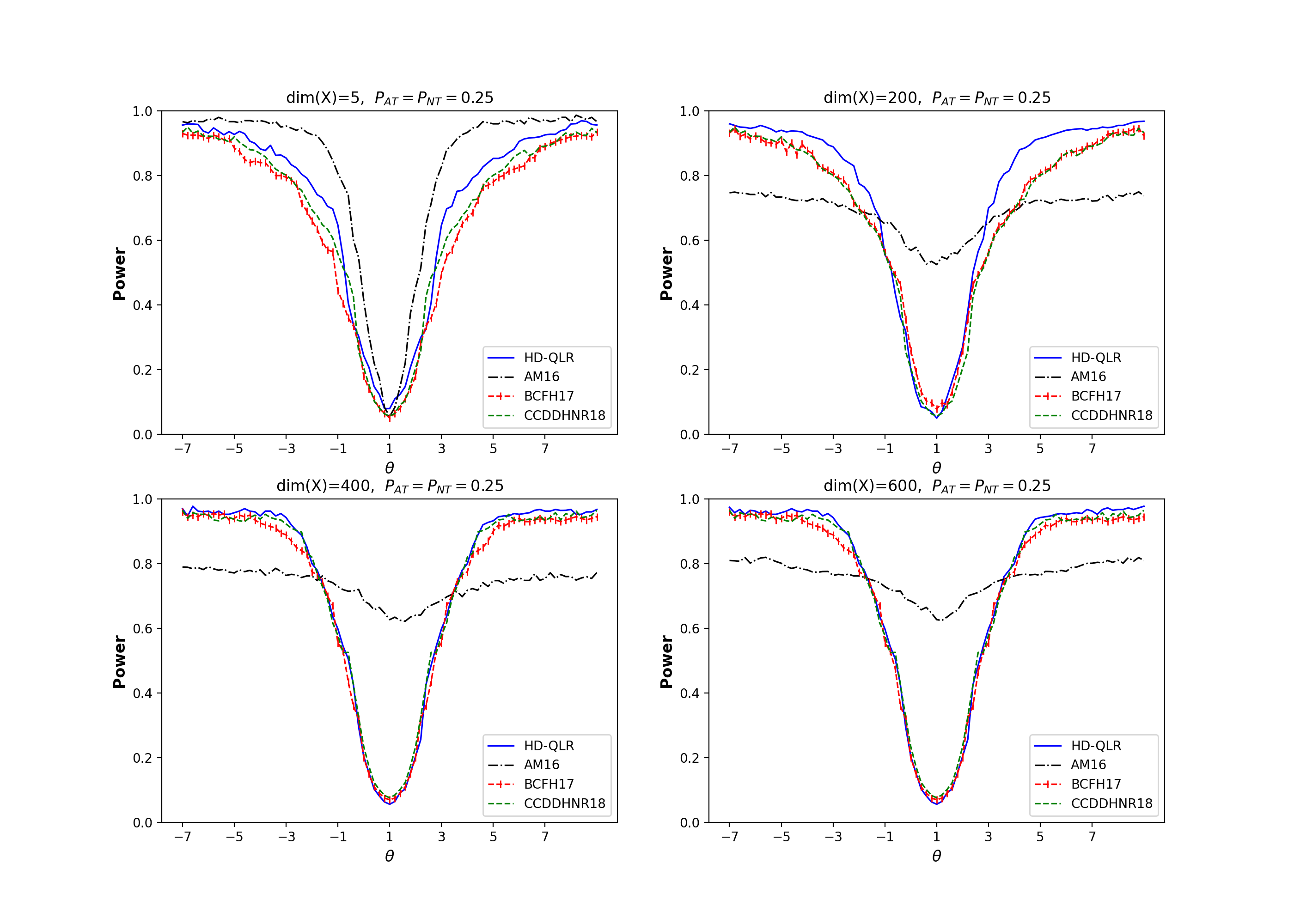
Figure 1: Power curves for HD-QLR (solid blue), AM16 (dash-dot black), BCFH17 (vertical marker red), and CCDDHNR18 (dashed green). Power of nominal 5% tests in strongly identified LATE design with the share of compliers being 0.5, and $N=500$ observations. Based on 2,500 replications, and for HD-QLR and AM16, 1,000 draws of conditional critical values were conducted. Upper left panel, number of covariates $\dim(X)=5$ ; upper right panel, $\dim(X)=200$; lower left panel, $\dim(X)=400$; lower right panel, $\dim(X)=600$.

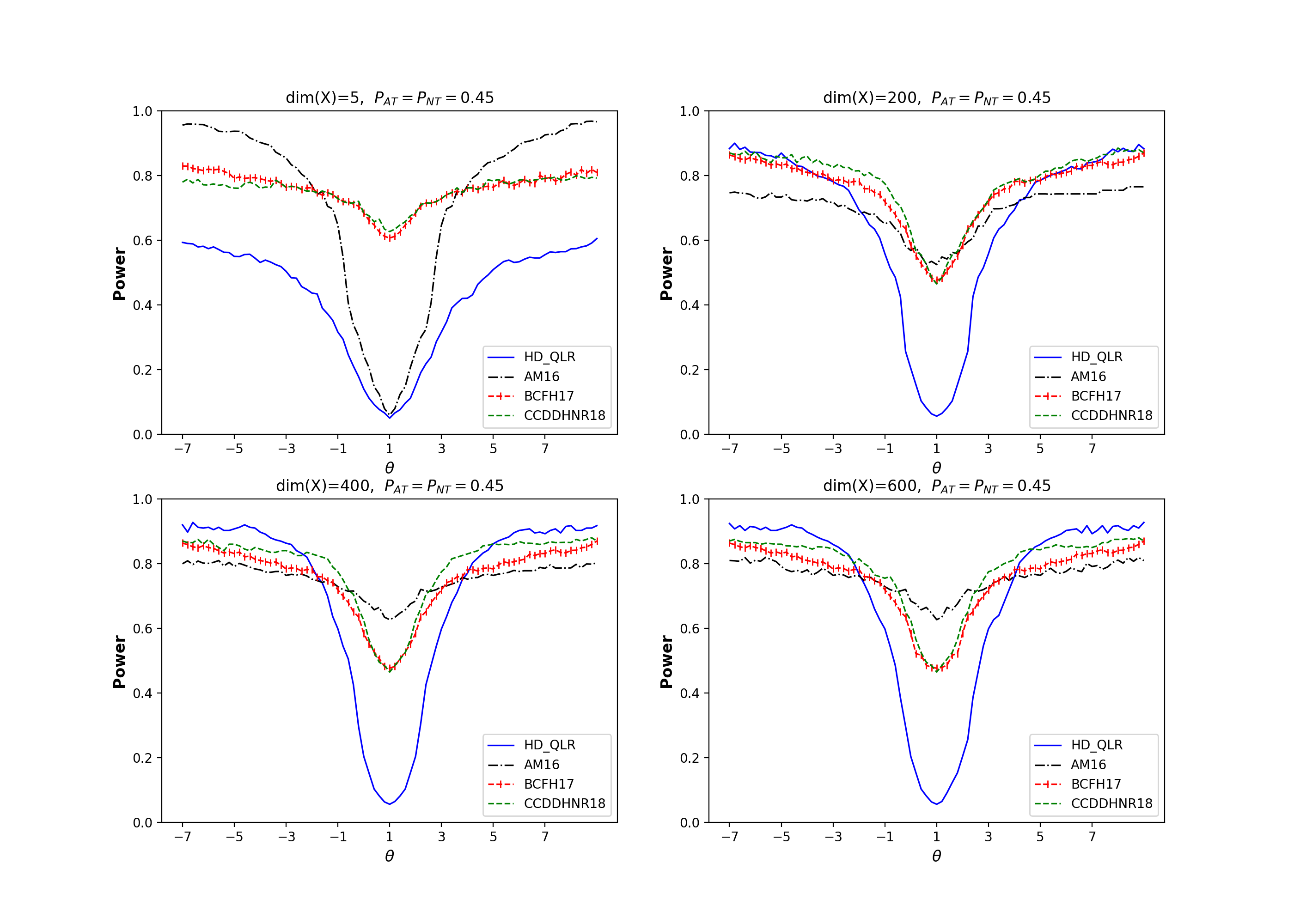
Figure 2: Power curves for HD-QLR (solid blue), AM16 (dash-dot black), BCFH17 (vertical marker red), and CCDDHNR18 (dashed green). Power of nominal 5% tests in weakly identified LATE design with the share of compliers being 0.1, and $N=500$ observations. Based on 2,500 replications, and for HD-QLR and AM16, 1,000 draws of conditional critical values were conducted. Upper left panel, number of covariates $\dim(X)=5$ ; upper right panel, $\dim(X)=200$; lower left panel, $\dim(X)=400$; lower right panel, $\dim(X)=600$.

Figure 3: Power curves for HD-QLR (solid blue), AM16 (dash-dot black), BCFH17 (vertical marker red), and CCDDHNR18 (dashed green). Power of nominal 5% tests in unidentified LATE design with the share of compliers being 0.02, and $N=500$ observations. Based on 2,500 replications, and for HD-QLR and AM16, 1,000 draws of conditional critical values were conducted. Upper left panel, number of covariates $\dim(X)=5$ ; upper right panel, $\dim(X)=200$; lower left panel, $\dim(X)=400$; lower right panel, $\dim(X)=600$.

Figure 1 depicts the strongly identified designs with the share of compliers being 0.5. The upper left figure represents the power curves for the “low-dimensional” LATE framework with $\dim(X)=5$. It is evident that all tests maintain satisfactory size control. In the remaining three figures, where $\dim(X)=$200, 400, and 600, our proposed method performs quite competitively with CCDDHNR18 and BCFH17, as all three methods are tailored for high-dimensional scenarios. While CCDDHNR18 and BCFH17 exhibit good power close to the null, their power slightly lags behind our proposed method in more distant alternatives. In contrast, AM16 suffers from significant size distortion and substantial power loss, revealing that the conditional QLR method is not robust against high dimensionality.

Figure 2 depicts the power curves within a weakly identified scenario where the share of compliers is 0.1. In the “low-dimensional” LATE model, both our proposed method and AM16 adeptly control size. However, AM16 exhibits significantly superior power performance over our method, since AM16 is specifically designed for models with low-dimensional nuisance parameters. Conversely, in the remaining designs, our method outperforms AM16 in both size control and power performance, highlighting the vulnerability of AM16 in high-dimensional contexts. Moreover, both CCDDHNR18 and BCFH17 face severe size distort and significant power loss across all designs, signaling their lack of robustness to weak identification.

Figure 3 presents results for scenarios where identification is completely absent with the proportion of compliers being 0.02. The patterns mirror those observed in weakly identified cases. Within the “low-dimensional” LATE framework, my proposed method and AM16 maintain correct size control, while the two machine-learning methods exhibit significant size distortion. For high-dimensional LATE designs, my method surpasses the other three conventional approaches in size control. The primary distinction between the unidentified and weakly identified scenarios is a notable reduction in power in the former. Furthermore, by juxtaposing the upper-left plots of Figure 1, 2 and 3, it becomes clear that our method adeptly maintains size control, not just in high-dimensional settings, but also in low-dimensional scenarios.

In summarizing our observations, we confirm that the proposed method consistently exhibits robustness against both weak identification and high dimensionality. In contrast, while CCDDHNR18 and BCFH17 exhibit robustness to high-dimensional settings, they struggle when facing weak identification. Likewise, AM16 shows robustness to weak identification but lacks robustness to high dimensionality.

5 Empirical Illustrations

5.1 The Impact of Railroad Access on City Growth

To demonstrate the methods outlined in the preceding sections, we revisit the IV estimations by Hornung (2015) concerning the impact of railroad access on city growth in 19th-century Prussia. In this study, straight-line corridors between major cities (nodes) are constructed, and whether a city is located on this line is used as an instrument for analysis. We compare our proposed high-dimensional QLR test with three other conventional methods: AM16, CCDDHNR18, and BCFH17, to infer the effect of railroad access. Our goal is to deepen our understanding of the conclusions presented in the literature. By conducting a new empirical analysis, we keep two econometric considerations in mind: 1. the inclusion of high-dimensional covariates to mitigate unobserved confoundedness, and 2. accounting for the weak identification issue in the data. For the first time, we report confidence intervals that are robust to weak identification and high dimensionality.

Consider the empirical model:

$$Y_{it}=D_{i}\theta_{0}+X_{i}^{\prime}\beta_{1}+\epsilon_{it},$$

$$D_{i}=\frac{\exp(Z_{i}\eta_{0}+X_{i}^{\prime}\beta_{2})}{1+\exp(Z_{i}\eta_{0}+X_{i}^{\prime}\beta_{2})}+v_{i},$$

where $Y_{it}$ denotes the urban population growth rate in city $i$ at time period $t$, $D_{i}$ is a dummy variable indicating whether there is a railroad access by 1848 in city $i$, and $Z_{i}$ denotes whether the city $i$ was located within a straight-line corridor between junction stations (nodes) in 1848. The covariates $X_{i}$ include a lagged dependent variable, distance to the closest node of railroad lines, age composition, primary education of the urban population, county-level concentration of large landholdings, access to main roads, rivers, and ports, pre-railroad city growth from 1831-1837, and the size of the civilian and military population in 1849.

Within this study, the exclusion restriction condition would be violated if the location of the cities in the straight-line corridor is associated with urban population growth through a channel other than the railroad. The author asserts that the exclusion restriction is satisfied in Hornung (2015, pg. 714), When estimating the reduce-form relationship of urban growth on location in the straight-line corridors, we find no correlation with the pre-railroad growth during 1831-1837. In the context of this study, it is noteworthy that the adoption of railroad technology by cities located on a straight line between two important cities was randomly assigned. This random assignment arises because the positioning of these cities along such lines was not intentionally controlled by any specific entity. In 19th-century Prussia, the government did not dictate railroad construction due to financial limitations. Instead, the decision fell to individual city councils negotiating with private railroad enterprises. Hence, each city had the autonomy to determine whether or not to proceed with railroad construction. Within this study, “compliers” refer to (1) cities situated on the straight line between two major cities AND eventually established a railroad station, and (2) cities NOT on such a line AND did NOT get a train station. The second part does not exist in this study as mentioned in Hornung (2015, pg. 731), One limitation of using IV estimation approaches lies in the fact that we can only estimate the local average treatment effect of railroad access for cities in the straight-line corridors. We implement the proposed method on the city-level railroad data from Hornung (2015). As outlined in Table 5 of Hornung (2015), the first-stage F-statistics vary between 26.46 and 38.29. This variation suggests instrument weakness based on the $tF$ critical value function proposed by Lee et al. (2022). We conducted a re-analysis by incorporating the polynomial and interaction terms of the original covariates, and present the results in Table 1. The sample spans from $N=898$ cities with the dimensionality of covariates $\dim(X)=204$, to $N=926$ cities with $\dim(X)=212$.

		(1)	(2)		(3)	(4)	(5)	(6)	(7)	(8)	(9)
$Y_{it}$: population		Main periods		Subperiods
growth rate		1831-37	49-71		49-52	52-55	55-58	58-61	61-64	64-67	67-71
Panel A: AM16
CI		[0.000,	[0.024,		[-0.015,	[0.006,	[0.030,	[0.012,	[0.021,	[0.012,	[0.018,
		0.018]	0.135]		0.081]	0.039]	0.150]	0.111]	0.090]	0.420]	0.155]
length of CI		0.018	0.111		0.096	0.033	0.120	0.099	0.069	0.408	0.137
Panel B: CCDDHNR18
CI		[-0.026,	[-0.004,		[-0.019,	[-0.014,	[-0.009,	[-0.016,	[-0.019,	[-0.014,	[-0.016,
		0.021]	0.033]		0.039]	0.035]	0.044]	0.030]	0.052]	0.039]	0.036]
length of CI		0.047	0.037		0.058	0.048	0.053	0.046	0.070	0.052	0.052
Panel C: BCFH17
CI		[-0.017,	[-0.003,		[-0.009,	[-0.006,	[-0.007,	[-0.008,	[-0.009,	[-0.018,	[-0.008,
		0.017]	0.026]		0.026]	0.023]	0.031]	0.020]	0.040]	0.041]	0.034]
length of CI		0.034	0.029		0.035	0.029	0.038	0.028	0.049	0.059	0.042
Panel D: HD-QLR with the number of folds K=4
CI		[-0.012,	[0.005,		[0.000,	[0.002,	[0.003,	[-0.001,	[0.003,	[-0.004,	[-0.002,
		0.012]	0.020]		0.021]	0.018]	0.027]	0.016]	0.029]	0.032]	0.023]
length of CI		0.024	0.015		0.021	0.016	0.024	0.017	0.026	0.033	0.024
Size N		898	906		929	924	914	926	924	919	919
dim(X)		204	212		212	212	212	212	212	212	212

Table 1: Displayed are confidence intervals (CI) and the length of confidence intervals for the coefficient of the railroad access. Panel A displays the results of AM16. Panel B presents the results obtained from CCDDHNR18. Panel C shows the results derived from BCFH17. Panel D showcases the results of the proposed HD-QLR test with the number $K=4$ folds for cross fitting. Estimation and inference results in panel B and D are based on 10 iterations of resampled cross fitting.

$Y_{it}$: population		Main periods		Subperiods
growth rate		1831-37	49-71		49-52	52-55	55-58	58-61	61-64	64-67	67-71
Panel A: HD-QLR with the number of folds K=3
CI		[-0.013,	[0.005,		[0.001,	[0.002,	[0.003,	[-0.002,	[0.003,	[-0.005,	[-0.003,
		0.011]	0.021]		0.023]	0.030]	0.026]	0.016]	0.030]	0.032]	0.022]
length of CI		0.024	0.016		0.023	0.018	0.023	0.018	0.027	0.037	0.025
Panel B: HD-QLR with the number of folds K=4
CI		[-0.012,	[0.005,		[0.000,	[0.002,	[0.003,	[-0.001,	[0.003,	[-0.004,	[-0.002,
		0.012]	0.020]		0.021]	0.018]	0.027]	0.016]	0.029]	0.032]	0.023]
length of CI		0.024	0.015		0.021	0.016	0.024	0.017	0.026	0.033	0.024
Size N		898	906		929	924	914	926	924	919	919
dim(X)		204	212		212	212	212	212	212	212	212

Table 2: Displayed are CI and the length of CI for the coefficient of the railroad access. Panel A showcases the results of the proposed HD-QLR test with the number $K=3$ folds for cross fitting. Panel B demonstrates the results of the proposed test with the number $K=4$ folds for cross fitting. Estimation and inference are based on 10 iterations of resampled cross fitting.

Table 1 summarizes the results. To emphasize the efficiency of the proposed method within the high-dimensional framework, we report the confidence intervals for the LATE estimates and the lengths of the confidence intervals. Panel A showcases results derived from AM16, which is not tailored for high-dimensional setting. Panel B details findings from CCDDHNR18, while Panel C displays results from BCFH17. Panel D features results from the proposed method, with $K=4$ folds for cross-fitting. Different columns report the results for several dependent variables across diverse time periods. Specifically, Columns (1) and (2) capture outcomes spanning two main periods: 1831-37 , and 1849-1871. Columns (3)-(9) depict findings across seven subperiods. To mitigate the uncertainty induced by sample splitting, we compute confidence intervals based on the average from ten randomized DML iterations following Chernozhukov et al. (2018a).

Upon comparing the results from Panel A and Panel D, it becomes apparent that our method produces more concise confidence intervals, between 17% to 92% shorter than those generated by AM16 in the subperiods specifications. Another notable finding is that several effects, considered statistically significant under AM16 without accounting for high-dimensional covariates, lose their significance when employing DML method to handle the high-dimensional covariates in the proposed method. In particular, the adoption of our proposed method leads to a loss of statistical significance for three out of the seven coefficients. As mentioned in page 714 about the second-stage results in Hornung (2015), We find a significant increase in urban population growth due to railroad access of 2.1 percentage points (with a standard deviation of 0.6 percentage points) during the period 1849-1871. Across all subperiods under consideration, the effect varies between 1.1 and 2.2 percentage points for a city that gained access by 1848.

When comparing the results across Panel B, Panel C, and Panel D, it is crucial to underscore that the confidence intervals derived from our proposed method exhibits notable reductions in length (ranging from 49% to 66% shorter) compared to those significantly larger intervals obtained from CCDDHNR18 and BCFH17, which lack robustness against weak identification.

To evaluate the impact of the number of folds on the results, Table 2 showcases the findings obtained from our proposed method, varying the number of folds. We observe that the confidence intervals remain consistent across Panel A and B, even with changes in the number of folds.

To robustly account for the weak identification issue in the high-dimensional context, we recommend researcher employ our proposed high-dimensional QLR method.

5.2 The Boundary Effects on Rental Prices

In this subsection, we reexamine the IV estimation by Ambrus et al. (2020) concerning the long-term consequences of the 1854 cholera outbreak on housing prices. The authors investigate the impacts of a cholera epidemic in a neighbor of 19th-century London on property values in 1864, a decade following the outbreak. Page 479 of Ambrus et al. (2020) presents the background information, In August 1854, St. James experienced a sudden outbreak of cholera when one of the 13 shallow wells that serviced the parish, the Broad Street pump, became contaminated with cholera bacteria… [So] residents were unaware they should stop using the local water source in order to avoid infection…. [Within] the Broad Street pump (BSP) catchment area, an estimated 16 percent of residents had contracted the disease and approximately 8 percent died.

In this context, $Y_{i}$ represents the log rental price of house $i$ in 1864. The variable $D_{i}$ is an indicator, set to 1 if house $i$ has at least one cholera death. Ambrus et al. (2020) use two instruments $Z_{i}$; we focus on their preferred instrument, which is an indicator for whether the property $i$ falls inside the Broad Street pump (BSP) catchment areas, which were the primary contaminated area during the outbreak. The controls $X_{i}$ comprise all house characteristic variables listed in Table 1 of Ambrus et al. (2020), such as distance to the closest pump, distance to the fire station, distance to the urinal, sewer access, among a total of 23 variables.

In this study, the “compliers” refer to (1) houses situated within the cholera-affected contaminated areas AND witnessed at least one cholera-related death, and (2) houses outside these contaminated zone AND did not experience any cholera fatalities. However, the latter category does not actually exist in the study since the authors limit the sample to properties within a certain distance of the BSP boundary.

Table B2 in Ambrus et al. (2020) presents IV estimates and confidence intervals of the effect of cholera-related deaths on rental prices in 1864. Notably, the first-stage F-statistics in the IV estimation are around 10, indicating weak identification according to the tF critical value function proposed by Lee et al. (2022). In light of this observation, we proceed with a reanalysis by incorporating all house characteristic variables listed in Table 1 in Ambrus et al. (2020). The dataset for our reanalysis consists of $N=467$ observations, with the dimensionality of the covariates $\dim(X)=23$. The original second-stage result is shown in page 493 in Ambrus et al. (2020), The IV results show that houses having at least one death report a 50 percent drop in rental value by 1854.

	AM16	CCDDHNR18	BCFH17	HD-QLR
CI	[-2.160,	[-1.132,	[-1.291,	[-1.080,
	-0.670]	0.406]	0.576]	0.035
length of CI	1.490	1.538	1.866	1.115

Table 3: Displayed are CI and the length of CI for the coefficient of the cholera-related deaths using four different approaches: AM16, CCDDHNR18, BCFH17, and the proposed HD-QLR. Estimation and inference results in CCDDHNR18 and HD-QLR are based on 10 iterations of resampled cross fitting with $K=4$ folds for cross fitting.

Table 3 presents the confidence intervals, and their lengths for four methodologies: AM16, CCDDHNR18, BCFH17, and our proposed HD-QLR. Our approach consistently delivers the shortest confidence interval. In contrast, the three other conventional methods yield relatively large confidence intervals. Noteworthy is that results deemed significant under AM16 lose their significance when using machine-learning methods to handle the high-dimensional covariates in the three alternative methods.

Given these insights, we advocate for our proposed HD-QLR method in high-dimensional models, especially when weak identification may be a concern.

6 Conclusion

In this paper, we address the challenge of weak identification within the LATE framework, especially in the presence of high-dimensional covariates. Our primary contribution lies in the introduction of an identification-robust inference method. This is paired with a user-friendly algorithm for inference and confidence interval construction for the LATE estimate. We validate the uniformly correct asymptotic size of our proposed method. Through simulation studies, our method exhibits superior size control and power performance in the finite sample, compared to the conventional identification-robust test and the conventional ML methods, particularly within a high-dimensional LATE framework with weak identification. Furthermore, we apply the proposed method to revisit the study by Hornung (2015) concerning the effect of railroad access on urban population growth. Our findings suggest our confidence intervals are substantially shorter than those from other conventional approaches. Similarly, when revisiting the study by Ambrus et al. (2020) on boundary effects on rental prices, we obtain exactly the same results as previously reported. Overall, our approach provides robustness against both weak identification and high dimensionality, underscoring its potential applicability for a wide range of empirical studies.

Appendix

Appendix A Useful Lemmas

For the convenience of readers, we provide the convergence rate for the nuisance parameter in the Lasso logistic and Lasso OLS models in Lemma 2 and 3.

Lemma 2.

(Convergence rate for Lasso with logistic model) Suppose that Assumption 4-7 hold. In addition, suppose that the penalty choice $\lambda_{1}=K_{1}\sqrt{N\log(pN)}$ and $\lambda_{2}=K_{2}\sqrt{N\log(pN)}$ for $K_{1},K_{2}>0$. Then with probability $1-o(1)$,

$$\|(\widehat{\beta}_{11},\widehat{\beta}_{12})-(\beta_{11}^{0},\beta_{12}^{0})\|\vee\|\widehat{\gamma}-\gamma^{0}\|\lesssim\sqrt{\frac{s_{N}\log(pN)}{N}}.$$

Lemma 3.

(Convergence rate for Lasso with OLS) Suppose that Assumption 4-7 hold. Moreover, suppose that the penalty choice $\lambda_{3}=K_{3}\sqrt{N\log(pN)}$ for $K_{3}>0$. Then with probability $1-o(1)$,

$$\|(\widehat{\beta}_{21},\widehat{\beta}_{22})-(\beta_{21}^{0},\beta_{22}^{0})\|\lesssim\sqrt{\frac{s_{N}\log(pN)}{N}}.$$

Appendix B Proofs of the Main Results

B.1 Proof of Theorem 1

Proof.

Without loss of generality, we define the size of each fold $I_{k}$ as $n=N/K$. For notation simplicity, we introduce the notation $[r]=\{1,\cdots,r\}$ for any $r\in\mathbb{N}$. Let us break down the proof into three steps. In Step 1, we demonstrate equation (3.10) and establish the asymptotic normality of $\widehat{\mathbb{G}}_{N}(\theta)$ over $P\in\mathcal{P}_{0}$, that is, the asymptotic normality of $(\widehat{\mathbb{G}}_{N}(\theta_{1}),\cdots,\widehat{\mathbb{G}}_{N}(\theta_{L}))$ for any $(\theta_{1},\cdots,\theta_{L})\in\Theta_{I}\times\cdots\times\Theta_{I}$. In step 2, we establish the asymptotic equicontinuity of $\widehat{\mathbb{G}}_{N}$ over $P\in\mathcal{P}_{0}$. Considering $\Theta_{I}$ is a subset of the compact set $\Theta$ and the score $\psi$ is continuous with respect to $\theta$, we infer $\Theta_{I}$ is both bounded and closed, implying its compactness. Given that $\Theta_{I}$ is a compact set, the proof of the weak convergence result is done. In Step 3, we prove that $\widehat{\Omega}(\theta_{1},\theta_{2})$ serves as a uniformly consistent estimator for the covariance function $\Omega(\theta_{1},\theta_{2})$ over $P\in\mathcal{P}_{0}$.

Step 1. In this step, we first establish equation (3.10). Becasue $K$ is a fixed integer and independent of $N$, it suffices to show that over $P\in\mathcal{P}_{0}$, for any $k\in[K]$,

$$\mathbb{E}_{n,k}[\psi(W;\theta,\widehat{\eta}_{k})]-{\mathrm{E}_{P}}[\psi(W;\theta,\widehat{\eta}_{k})]-\left(\mathbb{E}_{n,k}[\psi(W_{i},\theta,\eta_{0})]-{\mathrm{E}_{P}}[\psi(W;\theta,\eta_{0})]\right)=O_{p}(N^{-1/2}r_{N}^{\prime}).$$ (B.1)

For notation simplicity, we define $\mathbb{E}_{n,k}[f(W)]=n^{-1}\sum_{i\in I_{k}}f(W_{i})$. In order to show this, let us fix $k\in[K]$ and introduce an empirical process notation over $P\in\mathcal{P}_{0}$,

$$\mathbb{G}_{n,k}[\phi(W)]=\frac{1}{\sqrt{n}}\sum_{i\in I_{k}}(\phi(W_{i})-{\mathrm{E}_{P}}[\phi(W)]),$$

where $\phi$ is any $P_{N}$-integrable function of $W$. Then by triangle inequality, we have

$$\left\|\mathbb{E}_{n,k}[\psi(W;\theta,\widehat{\eta}_{k})]-{\mathrm{E}_{P}}[\psi(W;\theta,\widehat{\eta}_{k})]-\left(\mathbb{E}_{n,k}[\psi(W_{i},\theta,\eta_{0})]-{\mathrm{E}_{P}}[\psi(W;\theta,\eta_{0})]\right)\right\|$$ (B.2)

$$=n^{-1/2}\|\mathbb{G}_{n,k}[\psi(W;\theta,\widehat{\eta}_{k})]-\mathbb{G}_{n,k}[\psi(W;\theta,\eta_{0})]\|:=n^{-1/2}\mathcal{I}_{k3}.$$ (B.3)

Notice that, conditional on $(W_{i})_{i\in I_{k}^{c}}$, the estimator $\widehat{\eta}_{k}$ is non-stochastic. Then we have,

$${\mathrm{E}_{P}}[\mathcal{I}_{k3}^{2}|(W_{i})_{i\in I_{k}^{c}}] ={\mathrm{E}_{P}}\left[(\psi(W;\theta,\widehat{\eta}_{k})-\psi(W;\theta_{0},\eta_{0}))^{2}|(W_{i})_{i\in I_{k}^{c}}\right]$$

$$\leq\sup_{\eta\in\mathcal{T}_{N}}{\mathrm{E}_{P}}\left[(\psi(W;\theta,\eta)-\psi(W;\theta_{0},\eta_{0}))^{2}|(W_{i})_{i\in I_{k}^{c}}\right]$$

$$\leq\sup_{\eta\in\mathcal{T}_{N}}{\mathrm{E}_{P}}[(\psi(W;\theta,\eta)-\psi(W;\theta_{0},\eta_{0}))^{2}]\leq(r_{N}^{\prime})^{2}.$$

This completes the proof of equation (3.10). Combining (3.10) with the Lindeberg-Feller central limit theorem (CLT) and the Cramer-Wold device yields the asymptotic normality of $\widehat{\mathbb{G}}_{N}(\theta)$ for any $P\in\mathcal{P}_{0}$.

Step 2. In this step, we prove the asymptotic equicontinuity of $\widehat{\mathbb{G}}_{N}$ over $P\in\mathcal{P}_{0}$. The asymptotic equicontinuity of $\widehat{\mathbb{G}}_{N}$ can be stated as, for any $\epsilon_{1}>0$, and any $\theta_{1},\theta_{2}\in\Theta_{I}$ such that $|\theta_{1}-\theta_{2}|\leq\delta$,

$$\lim_{\delta\rightarrow 0}\underset{N\rightarrow\infty}{\lim}\sup_{P\in\mathcal{P}_{0}}P\left(|\widehat{\mathbb{G}}_{N}(\theta_{1})-\widehat{\mathbb{G}}_{N}(\theta_{2})|>\epsilon_{1}\right)=0.$$ (B.4)

By Markov’s inequity, for any $\epsilon_{1}>0$,

$$P\left(\left|\widehat{\mathbb{G}}_{N}(\theta_{1})-\widehat{\mathbb{G}}_{N}(\theta_{2})\right|>\epsilon_{1}\right)\leq\frac{1}{\epsilon_{1}}{\mathrm{E}_{P}}\left[\left|\widehat{\mathbb{G}}_{N}(\theta_{1})-\widehat{\mathbb{G}}_{N}(\theta_{2})\right|\right].$$

Thus, it suffices to show that for each $k\in[K]$.

$$\lim_{\delta\rightarrow 0}\underset{N\rightarrow\infty}{\lim}\sup_{P\in\mathcal{P}_{0}}\sqrt{N}{\mathrm{E}_{P}}\left[|\mathbb{E}_{n,k}[(\theta_{1}-\theta_{2})\psi^{a}(W;\widehat{\eta}_{k})]-{\mathrm{E}_{P}}[(\theta_{1}-\theta_{2})\psi^{a}(W;\widehat{\eta}_{k})]|\right]=0.$$ (B.5)

Note that

$$\operatorname{\text{E}}_{P}\left[\Big{|}\mathbb{E}_{n,k}[(\theta_{1}-\theta_{2})\psi^{a}(W;\widehat{\eta}_{k})]-{\mathrm{E}_{P}}[(\theta_{1}-\theta_{2})\psi^{a}(W;\widehat{\eta}_{k})]\Big{|}^{2}\right]\leq n^{-1}\delta^{2}{\mathrm{E}_{P}}\left[\psi^{a}(W;\widehat{\eta}_{k})^{2}\right]\leq n^{-1}\delta^{2}c_{1}^{2},$$

which implies the equation (B.5). Thus, we complete the proof of the asymptotic equicontinuity of $\widehat{\mathbb{G}}_{N}$ over $P\in\mathcal{P}_{0}$.

Step 3. In this step, we first show $\widehat{\Omega}(\theta_{1},\theta_{2})=\Omega(\theta_{1},\theta_{2})+O_{P}(\rho_{N})$, and then we show $\widehat{\Omega}$ is a uniformly consistent estimator for $\Omega$ over $P\in\mathcal{P}_{0}$. To prove the first part, it suffices to show that over $P\in\mathcal{P}_{0}$ and each $k\in[K]$,

$$\mathcal{I}_{k}=\left|\mathbb{E}_{n,k}[\psi(W;\theta_{1},\widehat{\eta}_{k})\psi(W;\theta_{2},\widehat{\eta}_{k})]-{\mathrm{E}_{P}}[\psi(W;\theta_{1},\eta_{0})\psi(W;\theta_{2},\eta_{0})]\right|=O_{p}(\rho_{N}),\quad and$$

$$\mathcal{I}_{k}^{\prime}=\left|\mathbb{E}_{n,k}[\psi(W;\theta,\widehat{\eta}_{k})]-{\mathrm{E}_{P}}[\psi(W;\theta,\eta_{0})]\right|=O_{p}(\rho_{N}).$$

Note that by triangle inequality, we have $\mathcal{I}_{k}\leq\mathcal{I}_{k1}+\mathcal{I}_{k2},$ and $\mathcal{I}_{k}^{\prime}\leq\mathcal{I}_{k4}+\mathcal{I}_{k5},$ where

$$\mathcal{I}_{k1}=\left|\mathbb{E}_{n,k}[\psi(W;\theta_{1},\widehat{\eta}_{k})\psi(W;\theta_{2},\widehat{\eta}_{k})]-\mathbb{E}_{n,k}[\psi(W;\theta_{1},\eta_{0})\psi(W;\theta_{2},\eta_{0})]\right|,$$

$$\mathcal{I}_{k2}=\left|\mathbb{E}_{n,k}[\psi(W;\theta_{1},\eta_{0})\psi(W;\theta_{2},\eta_{0})]-{\mathrm{E}_{P}}[\psi(W;\theta_{1},\eta_{0})\psi(W;\theta_{2},\eta_{0})]\right|,$$

$$\mathcal{I}_{k4}=\left|\mathbb{E}_{n,k}[\psi(W;\theta,\widehat{\eta}_{k})]-\mathbb{E}_{n,k}[\psi(W;\theta,\eta_{0})]\right|,\quad\mathcal{I}_{k5}=\left|\mathbb{E}_{n,k}[\psi(W;\theta,\eta_{0})]-{\mathrm{E}_{P}}[\psi(W;\theta,\eta_{0})]\right|.$$

First, we bound $\mathcal{I}_{k2}$ and $\mathcal{I}_{k5}$. Note that for $q\geq 4$, we have

$${\mathrm{E}_{P}}[\mathcal{I}^{2}_{k2}]\leq\sup_{P\in\mathcal{P}_{0}}n^{-1}{\mathrm{E}_{P}}[\psi(W;\theta,\eta_{0})^{4}]\leq n^{-1}c_{1}^{4},$$

$${\mathrm{E}_{P}}[\mathcal{I}_{k5}^{2}]\leq\sup_{P\in\mathcal{P}_{0}}n^{-1}{\mathrm{E}_{P}}[\psi(W;\theta,\eta_{0})^{2}]\leq n^{-1}c_{1}^{2},$$

where the last inequality follows from Assumption 2 (ii) and Jensen’s inequality. Next, we try to bound $\mathcal{I}_{k1}$.

$$\mathcal{I}_{k1} =\left|\frac{1}{n}\sum_{i\in I_{k}}\left[\psi(W_{i};\theta_{1},\widehat{\eta}_{k})\psi(W_{i};\theta_{2},\widehat{\eta}_{k})-\psi(W_{i};\theta_{1},\eta_{0})\psi(W_{i};\theta_{2},\eta_{0})\right]\right|$$

$$\leq\frac{1}{n}\sum_{i\in I_{k}}\big{|}\psi(W_{i};\theta_{1},\widehat{\eta}_{k})\psi(W_{i};\theta_{2},\widehat{\eta}_{k})-\psi(W_{i};\theta_{1},\eta_{0})\psi(W_{i};\theta_{2},\eta_{0})\big{|}$$

$$\leq\frac{2}{n}\sum_{i\in I_{k}}\sup_{\theta\in\Theta_{I}}\sup_{\eta\in\mathcal{T}_{N}}\Big{(}\left|\psi(W_{i};\theta,\widehat{\eta}_{k})-\psi(W_{i};\theta,\eta_{0})\right|\times|\psi(W_{i};\theta,\eta)|\Big{)}$$

$$\leq\frac{2}{n}\sum_{i\in I_{k}}\Big{(}\sup_{\theta\in\Theta_{I}}\left(\psi(W_{i};\theta,\widehat{\eta}_{k})-\psi(W_{i};\theta,\eta_{0})\right)^{2}\Big{)}^{1/2}\times\Big{(}\sup_{\theta\in\Theta_{I}}\sup_{\eta\in\mathcal{T}_{N}}\frac{2}{n}\sum_{i\in I_{k}}\psi(W_{i};\theta,\eta)^{2}\Big{)}^{1/2}$$

and the conditional expectation of the first term given $(W_{i})_{i\in I_{k}^{c}}$ on the event that $\widehat{\eta}_{k}\in\mathcal{T}_{N}$ is equal to

$$\sup_{P\in\mathcal{P}_{0}}{\mathrm{E}_{P}}\left[\|\psi(W;\theta,\widehat{\eta}_{k})-\psi(W;\theta,\eta_{0})\|^{2}|(W_{i})_{i\in I_{k}^{c}}\right]\leq\sup_{\eta\in\mathcal{T}_{N},P\in\mathcal{P}_{0}}{\mathrm{E}_{P}}\left[\|\psi(W;\theta,\eta)-\psi(W;\theta,\eta_{0})\|^{2}|(W_{i})_{i\in I_{k}^{c}}\right]=r_{N}^{\prime 2},$$

Because the event that $\widehat{\eta}_{k}\in\mathcal{T}_{N}$ holds with probability $1-\Delta_{N}=1-o(1)$, it follows that $\mathcal{I}_{k1}=O_{P}(r_{N}^{\prime})=O_{P}(\delta_{N})$. Since $\mathcal{I}_{k2}=O_{P}(N^{-1/2})$ and $\delta_{N}\geq N^{-1/2}$, we have $\mathcal{I}_{k}=O_{p}(\rho_{N})$ with $\rho_{N}\lesssim\delta_{N}$. Then we try to bound $\mathcal{I}_{k4}$.

$$\mathcal{I}_{k4}= \left|\frac{1}{n}\sum_{i\in I_{k}}\left[\psi(W_{i};\theta,\widehat{\eta}_{k})-\psi(W_{i};\theta,\eta_{0})\right]\right|\leq\frac{1}{n}\sum_{i\in I_{k}}\left|\psi(W_{i};\theta,\widehat{\eta}_{k})-\psi(W_{i};\theta,\eta_{0})\right|$$

$$\leq\sup_{\theta\in\Theta_{I}}\left(\frac{1}{n}\sum_{i\in I_{k}}\left\|\psi(W_{i};\theta,\widehat{\eta}_{k})-\psi(W_{i};\theta,\eta_{0})\right\|^{2}\right)^{1/2}.$$

By using the similar argument that we use to bound $\mathcal{I}_{k1}$, we obtain $\mathcal{I}_{k4}=O_{P}(r_{N}^{\prime})$. Therefore, we have $\mathcal{I}_{k}^{\prime}=O_{P}(\rho_{N})$ with $\rho_{N}\lesssim\delta_{N}$. This completes the proof of $\widehat{\Omega}(\theta_{1},\theta_{2})=\Omega(\theta_{1},\theta_{2})+O_{P}(\rho_{N})$. To prove $\widehat{\Omega}$ is a uniformly consistent estimator of $\Omega$ over $P\in\mathcal{P}_{0}$, we need to show that for any $\varepsilon_{2}>0$, and any $\theta_{1},\theta_{2},\theta_{1}^{\prime},\theta_{2}^{\prime}\in\Theta_{I}$ such that $|\theta_{1}-\theta_{1}^{\prime}|\leq\delta_{1}$ and $|\theta_{2}-\theta_{2}^{\prime}|\leq\delta_{2}$, we have

$$\lim_{\delta_{1},\delta_{2}\rightarrow 0}\underset{N\rightarrow\infty}{\lim}\sup_{P\in\mathcal{P}_{0}}P\left(|\widehat{\Omega}(\theta_{1},\theta_{2})-\widehat{\Omega}(\theta_{1}^{\prime},\theta_{2}^{\prime})|>\epsilon_{2}\right)=0.$$

By Markov’s inequality, for any $\varepsilon_{2}>0$,

$$P\left(|\widehat{\Omega}(\theta_{1},\theta_{2})-\widehat{\Omega}(\theta_{1}^{\prime},\theta_{2}^{\prime})|>\epsilon_{2}\right)\leq\frac{1}{\varepsilon_{2}}{\mathrm{E}_{P}}\left[\left|\widehat{\Omega}(\theta_{1},\theta_{2})-\widehat{\Omega}(\theta_{1}^{\prime},\theta_{2}^{\prime})\right|\right].$$

Thus, it suffices to show that pver $P\in\mathcal{P}_{0}$, for each $k\in[K]$,

$$\mathcal{I}_{k6}:={\mathrm{E}_{P}}\left[\left|\mathbb{E}_{n,k}[\psi(W;\theta_{1},\widehat{\eta}_{k})\psi(W;\theta_{2},\widehat{\eta}_{k})]-\mathbb{E}_{n,k}[\psi(W;\theta_{1}^{\prime},\widehat{\eta}_{k})\psi(W;\theta_{2}^{\prime},\widehat{\eta}_{k})]\right|\right]=0,$$

as $n\rightarrow\infty,\delta_{1},\delta_{2}\rightarrow 0$. Note that

$$\mathcal{I}_{k6} \leq\sup_{P\in\mathcal{P}_{0}}{\mathrm{E}_{P}}\left[\mathbb{E}_{n}\left[\left|\psi(W;\theta_{1},\widehat{\eta}_{k})-\psi(W;\theta_{1}^{\prime},\widehat{\eta}_{k})\right|\cdot\left|\psi(W;\theta_{2},\widehat{\eta}_{k})\right|\right]+\mathbb{E}_{n}\left[\left|\psi(W;\theta_{2},\widehat{\eta}_{k})-\psi(W;\theta_{2}^{\prime},\widehat{\eta}_{k})\right|\cdot\left|\psi(W;\theta_{1}^{\prime},\widehat{\eta}_{k})\right|\right]\right]$$

$$=\sup_{P\in\mathcal{P}_{0}}{\mathrm{E}_{P}}\left[\mathbb{E}_{n}\left[\left|\psi^{a}(W;\widehat{\eta}_{k})\cdot(\theta_{1}-\theta_{1}^{\prime})\right|\cdot\left|\psi(W;\theta_{2},\widehat{\eta}_{k})\right|\right]\right]+{\mathrm{E}_{P}}\left[\mathbb{E}_{n}\left[\left|\psi^{a}(W;\widehat{\eta}_{k})\cdot(\theta_{2}-\theta_{2}^{\prime})\right|\cdot\left|\psi(W;\theta_{1}^{\prime},\widehat{\eta}_{k})\right|\right]\right]$$

$$\leq\sup_{P\in\mathcal{P}_{0}}({\mathrm{E}_{P}}\left[\psi^{a}(W;\widehat{\eta}_{k})^{2}\cdot(\theta_{1}-\theta_{1}^{\prime})^{2}\right])^{1/2}\cdot\left({\mathrm{E}_{P}}\left[\psi(W;\theta_{2},\widehat{\eta}_{k})^{2}\right]\right)^{1/2}$$

$$+\sup_{P\in\mathcal{P}_{0}}({\mathrm{E}_{P}}\left[\psi^{a}(W;\widehat{\eta}_{k})^{2}\cdot(\theta_{2}-\theta_{2}^{\prime})^{2}\right])^{1/2}\cdot\left({\mathrm{E}_{P}}\left[\psi(W;\theta_{1}^{\prime},\widehat{\eta}_{k})^{2}\right]\right)^{1/2}$$

$$\leq\delta_{1}\sup_{P\in\mathcal{P}_{0}}({\mathrm{E}_{P}}\left[\psi^{a}(W;\widehat{\eta}_{k})^{4}\right])^{1/4}\cdot\left({\mathrm{E}_{P}}\left[\psi(W;\theta_{2},\widehat{\eta}_{k})^{4}\right]\right)^{1/4}+\delta_{2}\sup_{P\in\mathcal{P}_{0}}({\mathrm{E}_{P}}\left[\psi^{a}(W;\widehat{\eta}_{k})^{4}\right])^{1/4}\cdot\left({\mathrm{E}_{P}}\left[\psi(W;\theta_{1}^{\prime},\widehat{\eta}_{k})^{4}\right]\right)^{1/4}$$

$$\leq(\delta_{1}+\delta_{2})c_{1}^{2},$$

where the second inequality follows from Cauchy-Schwarz inequality, the third inequality follows from Jensen’s inequality, and the last one is from Assumption 2 (ii). It is obvious that $\lim_{\delta_{1},\delta_{2}\rightarrow 0}\mathcal{I}_{k6}=0$. Therefore, $\widehat{\Omega}$ is a uniformly consistent estimator of $\Omega$ over $P\in\mathcal{P}_{0}$. This completes the whole proof of Theorem 1.

∎

B.2 Proof of Theorem 2

Proof.

As long as we show Lemma 1 holds, the proof of Theorem 2 is done. Let us define $\mathcal{T}_{N}$ as the set of all $\eta=(g,m,p)$ consisting of $P$-square-integrable function $g,m$ and $p$ such that

$$\|\eta-\eta_{0}\|_{P,q}\leq c_{1},\quad\|\eta-\eta_{0}\|_{P,2}\leq\delta_{N}.$$

We proceed in four steps.

Step 1. We first verify the Assumption 1 that the AR-type Neyman orthogonal LATE score in (2.5) satisfies the moment condition (3.1) and the Neyman orthogonality condition (3.2). It can be easily verified that moment condition is satisfied. The Gateaux derivative in the direction $\eta-\eta_{0}=(g-g_{0},m-m_{0},p-p_{0})$ is given by

$$\partial_{\eta}{\mathrm{E}_{P}}\left[\psi(W;\theta_{0},\eta)\right]\Big{|}_{\eta=\eta_{0}}(\eta-\eta_{0})$$

$$={\mathrm{E}_{P}}\left[\left(1-\frac{Z}{p_{0}(X)}\right)(g(1,X)-g_{0}(1,X))\right]-{\mathrm{E}_{P}}\left[\left(1-\frac{1-Z}{1-p_{0}(X)}\right)(g(0,X)-g_{0}(0,X))\right]$$

$$-\theta_{0}{\mathrm{E}_{P}}\left[\left(1-\frac{Z}{p_{0}(X)}\right)(m(1,X)-m_{0}(1,X))\right]+\theta_{0}{\mathrm{E}_{P}}\left[\left(1-\frac{1-Z}{1-p_{0}(X)}\right)(m(0,X)-m_{0}(0,X))\right]$$

$$+{\mathrm{E}_{P}}\left[\left(\frac{\theta_{0}Z(D-m_{0}(1,X))-Z(Y-g_{0}(1,X))}{p_{0}(X)^{2}}+\frac{\theta_{0}(1-Z)(D-m_{0}(0,X))-(1-Z)(Y-g_{0}(0,X))}{(1-p_{0}(X))^{2}}\right)\times(p(X)-p_{0}(X))\right]$$

$$=0,$$

where the last equality follows from the law of iterated expectations and

$${\mathrm{E}_{P}}[Z|X]=p_{0}(X),\quad{\mathrm{E}_{P}}[Z(Y-g_{0}(1,X))|X,Z]=0,\quad{\mathrm{E}_{P}}[Z(D-m_{0}(1,X))|X,Z]=0,$$ (B.6)

$${\mathrm{E}_{P}}[1-Z|X]=1-p_{0}(X),\quad{\mathrm{E}_{P}}[(1-Z)(Y-g_{0}(0,X))|X,Z]=0,\quad{\mathrm{E}_{P}}[(1-Z)(D-m_{0}(0,X))|X,Z]=0.$$

Referring to the definitions of the AR-type score for the LATE in (2.5) and linear orthogonal score in (3.9), we have

$$\psi^{b}(W;\eta)=g(1,X)-g(0,X)+\frac{Z(Y-g(1,X))}{p(X)}-\frac{(1-Z)(Y-g(0,X))}{1-p(X)},$$

$$\psi^{a}(W;\eta)=-m(1,X)+m(0,X)-\frac{Z(D-m(1,X))}{p(X)}+\frac{(1-Z)(D-m(0,X))}{1-p(X)}.$$

Then we have $\psi(W;\theta,\eta)=\psi^{b}(W;\eta)+\theta\times\psi^{a}(W;\eta)$. Therefore, all the conditions in Assumption 1 hold.

Step 2. Next, let us verify Assumption 2 (iii). Note that

$${\mathrm{E}_{P}}\left[\psi(W;\theta,\eta_{0})^{2}\right]={\mathrm{E}_{P}}\big{[}\left(g_{0}(1,X)-g_{0}(0,X)-\theta(m_{0}(1,X)-m_{0}(0,X))\right)^{2}\big{]}$$

$$+{\mathrm{E}_{P}}\Big{[}\Big{(}\frac{Z(Y-g_{0}(1,X))}{p_{0}(X)}-\frac{(1-Z)(Y-g_{0}(0,X))}{1-p_{0}(X)}-\theta\big{(}\frac{Z(D-m_{0}(1,X))}{p_{0}(X)}-\frac{(1-Z)(D-m_{0}(0,X))}{1-p_{0}(X)}\big{)}\Big{)}^{2}\Big{]}$$

$$\geq{\mathrm{E}_{P}}\Big{[}\Big{(}\frac{Z(Y-g_{0}(1,X))}{p_{0}(X)}-\frac{(1-Z)(Y-g_{0}(0,X))}{1-p_{0}(X)}\Big{)}^{2}\Big{]}-\theta^{2}{\mathrm{E}_{P}}\Big{[}\Big{(}\frac{Z(D-m_{0}(1,X))}{p_{0}(X)}-\frac{(1-Z)(D-m_{0}(0,X))}{1-p_{0}(X)}\Big{)}^{2}\Big{]}$$

$$\geq{\mathrm{E}_{P}}\left[\frac{Z^{2}(Y-g_{0}(1,X))^{2}}{p_{0}(X)^{2}}\right]+{\mathrm{E}_{P}}\left[\frac{(1-Z)^{2}(Y-g_{0}(0,X))^{2}}{(1-p_{0}(X))^{2}}\right]$$

$$\geq\frac{{\mathrm{E}_{P}}\left[Z(Y-g_{0}(1,X))^{2}+(1-Z)(Y-g_{0}(0,X))^{2}\right]}{(1-\varepsilon)^{2}}$$

$$=\frac{{\mathrm{E}_{P}}[u^{2}]}{(1-\varepsilon)^{2}}\geq\frac{c_{0}^{2}}{(1-\varepsilon)^{2}},$$

where the first equality holds since the interaction term equals to zero by the equations in (B.6), the third inequality follows from the facts that $\varepsilon\leq p_{0}(X)\leq 1-\varepsilon$, and the last equality follows from Assumption 3 (iv). Thus the Assumption 2 (iii) is satisfied.

Step 3. Next, we verify Assumption 2 (i). By Lemmas 2 and 3 invoked by Assumption 3-7, with probability $1-o(1)$,

$$\|(\widehat{\beta}_{11},\widehat{\beta}_{12})-(\beta_{11}^{0},\beta_{12}^{0})\|\vee\|(\widehat{\beta}_{21},\widehat{\beta}_{22})-(\beta_{21}^{0},\beta_{22}^{0})\|\vee\|\widehat{\gamma}-\gamma^{0}\|\lesssim\sqrt{\frac{s_{N}\log(pN)}{N}}.$$

The proof of Lemmas 2 and 3 are given in Section B.4 and B.5. Thus Assumption 2 (i) is satisfied.

Step 4. Next, let us verify the condition in Assumption 2 (ii). Note that

$$\|g_{0}(D,X)\|_{P,q} =({\mathrm{E}_{P}}[|g_{0}(D,X)|^{q}])^{1/q}$$

$$\geq({\mathrm{E}_{P}}[|g_{0}(1,X)|^{q}P(D=1|X)+|g_{0}(0,X)|^{q}P(D=0|X)])^{1/q}$$

$$\geq\varepsilon^{1/q}({\mathrm{E}_{P}}[|g_{0}(1,X)|^{q}]+{\mathrm{E}_{P}}[|g_{0}(0,X)|^{q}])^{1/q}$$

$$\geq\varepsilon^{1/q}({\mathrm{E}_{P}}[|g_{0}(1,X)|^{q}]\vee{\mathrm{E}_{P}}[|g_{0}(0,X)|^{q}])^{1/q}$$

$$\geq\varepsilon^{1/q}(\|g_{0}(1,X)\|_{P,q}\vee\|g_{0}(0,X)\|_{P,q}).$$

Since $\|g_{0}(D,X)\|_{P,q}\leq\|Y\|_{P,q}\leq c_{1}$ by Assumption 3, we have

$$\|g_{0}(1,X)\|_{P,q}\leq c_{1}/\varepsilon^{1/q},\text{and}\|g_{0}(0,X)\|_{P,q}\leq c_{1}/\varepsilon^{1/q}.$$

By using similar arguments, we obtain

$$\|g(1,X)-g_{0}(1,X)\|_{P,q}\leq c_{1}/\varepsilon^{1/q},\quad\|g(0,X)-g_{0}(0,X)\|_{P,q}\leq c_{1}/\varepsilon^{1/q},$$ (B.7)

$$\|m_{0}(1,X)\|_{P,q}\leq 1/\varepsilon^{1/q},\quad\|m_{0}(0,X)\|_{P,q}\leq 1/\varepsilon^{1/q},$$

$$\|m(1,X)-m_{0}(1,X)\|_{P,q}\leq c_{1}/\varepsilon^{1/q},\quad\|m(0,X)-m_{0}(0,X)\|_{P,q}\leq c_{1}/\varepsilon^{1/q},$$

since $\|m_{0}(D,X)\|_{P,q}\leq 1$, $\|g(D,X)-g_{0}(D,X)\|_{P,q}\leq c_{1}$, and $\|m(Z,X)-m_{0}(Z,X)\|_{P,q}\leq c_{1}$. By calculation, we obtain

$$\|\psi^{a}(W;\eta)\|_{P,q}\leq(1+\varepsilon^{-1})(\|m(1,X)\|_{P,q}+\|m(0,X)\|_{P,q})+2/\varepsilon$$

$$\leq(1+\varepsilon^{-1})(\|m(1,X)-m_{0}(1,X)\|_{P,q}+\|m_{0}(1,X)\|_{P,q}+\|m(0,X)-m_{0}(0,X)\|_{P,q}+\|m_{0}(0,X)\|_{P,q})+2/\varepsilon$$

$$\leq(1+\varepsilon^{-1})(2c_{1}\varepsilon^{-1/q}+2\varepsilon^{-1/q})+2\varepsilon^{-1}:=c_{\varepsilon 1},$$

$$\|\psi^{b}(W;\eta)\|_{P,q}\leq(1+\varepsilon^{-1})(\|g(1,X)\|_{P,q}+\|g(0,X)\|_{P,q})+2\|Y\|_{P,q}/\varepsilon$$

$$\leq(1+\varepsilon^{-1})(2c_{1}\varepsilon^{-1/q}+2\varepsilon^{-1/q})+2c_{1}\varepsilon^{-1}:=c_{\varepsilon 2},$$

where $c_{\varepsilon 1}$ and $c_{\varepsilon 2}$ are constants related with $\varepsilon$ instead of $N$. Note that this completes the verification of Assumption 2 (b) Therefore, under the null, we have

$$({\mathrm{E}_{P}}[\|\psi(W;\theta,\eta)\|^{q}])^{1/q}=\|\psi(W;\theta,\eta)\|_{P,q}\leq\|\psi(W;\theta,\eta)-\psi(W;\theta_{0},\eta)\|_{P,q}+\|\psi(W;\theta_{0},\eta)\|_{P,q}$$

$$\leq|\theta-\theta_{0}|\times\|\psi^{a}(W;\eta)\|_{P,q}+\|\psi^{b}(W;\eta)\|_{P,q}+|\theta_{0}|\times\|\psi^{a}(W;\eta)\|_{P,q}$$

$$\leq|\theta-\theta_{0}|c_{\varepsilon 1}+c_{\varepsilon 2}+|\theta_{0}|c_{\varepsilon 1}\lesssim 1,$$

where the last inequality need the assumption that $\Theta$ is a compact set by Assumption 3 (vi). This completes the verification of Assumption 2 (ii) (a).

Next, let us verify the condition in Assumption 2 (ii) (c). For any $\eta=(g,m,p)$, by the triangle inequality,

$$({\mathrm{E}_{P}}[\|\psi(W;\theta,\eta)-\psi(W;\theta,\eta_{0})\|^{2}])^{1/2}=\|\psi(W;\theta,\eta)-\psi(W;\theta,\eta_{0})\|_{P,2}\leq\mathcal{I}_{1}+\mathcal{I}_{2}+\mathcal{I}_{3}+\mathcal{I}_{4},$$

where

$$\mathcal{I}_{1}:=\|g(1,X)-g_{0}(1,X)\|_{P,2}+\|g(0,X)-g_{0}(0,X)\|_{P,2},$$

$$\mathcal{I}_{2}:=|\theta|\times\left(\|m(1,X)-m_{0}(1,X)\|_{P,2}+\|m(0,X)-m_{0}(0,X)\|_{P,2}\right),$$

$$\mathcal{I}_{3}:=\left\|\frac{Z(Y-g(1,X))}{p(X)}-\frac{Z(Y-g_{0}(1,X))}{p_{0}(X)}\right\|_{P,2}+\left\|\frac{(1-Z)(Y-g(0,X))}{1-p(X)}-\frac{(1-Z)(Y-g_{0}(0,X))}{1-p_{0}(X)}\right\|_{P,2},$$

$$\mathcal{I}_{4}:=|\theta|\times\left(\left\|\frac{Z(D-m(1,X))}{p(X)}-\frac{Z(D-m_{0}(1,X))}{p_{0}(X)}\right\|_{P,2}+\left\|\frac{(1-Z)(D-m(0,X))}{1-p(X)}-\frac{(1-Z)(D-m_{0}(0,X))}{1-p_{0}(X)}\right\|_{P,2}\right).$$

By using the similar argument as the one in obtaining equation (B.7), we have

$$\|g(1,X)-g_{0}(1,X)\|_{P,2}\leq\delta_{N}/\varepsilon^{1/q},\quad\|g(0,X)-g_{0}(0,X)\|_{P,2}\leq\delta_{N}/\varepsilon^{1/q},$$

$$\|m(1,X)-m_{0}(1,X)\|_{P,2}\leq\delta_{N}/\varepsilon^{1/q},\quad\|m(0,X)-m_{0}(0,X)\|_{P,2}\leq\delta_{N}/\varepsilon^{1/q}.$$

so $\mathcal{I}_{1}\leq 2\delta_{N}/\varepsilon^{1/q}$ and $\mathcal{I}_{2}\lesssim 2\delta_{N}/\varepsilon^{1/q}$. To bound $\mathcal{I}_{3}$, we have

$$\mathcal{I}_{3} \leq\varepsilon^{-2}\times\Big{(}\|Zp_{0}(X)(Y-g(1,X))-Zp(X)(Y-g_{0}(1,X))\|_{P,2}$$

$$+\|(1-Z)(1-p_{0}(X))(Y-g(0,X))-(1-Z)(1-p(X))(Y-g_{0}(0,X))\|_{P,2}\Big{)}$$

$$\leq\varepsilon^{-2}\times\Big{(}\|p_{0}(X)(u+g_{0}(1,X)-g(1,X))-p(X)u\|_{P,2}$$

$$+\|(1-p_{0}(X))(u+g_{0}(0,X)-g(0,X))-(1-p(X))u\|_{P,2}\Big{)}$$

$$\leq\varepsilon^{-2}\times\Big{(}\|p_{0}(X)(g_{0}(1,X)-g(1,X))\|_{P,2}+\|(p(X)-p_{0}(X))u\|_{P,2}$$

$$+\|(1-p_{0}(X))(g_{0}(0,X)-g(0,X))\|+\|(p(X)-p_{0}(X))u\|_{P,2}\Big{)}$$

$$\leq\varepsilon^{-2}\times\Big{(}\|(g_{0}(1,X)-g(1,X))\|_{P,2}+\sqrt{c_{1}}\|p(X)-p_{0}(X)\|_{P,2}$$

$$+\|(g_{0}(0,X)-g(0,X))\|+\sqrt{c_{1}}\|p(X)-p_{0}(X)\|_{P,2}\Big{)}$$

$$\leq\varepsilon^{-2}\times(2/\varepsilon^{1/q}+2\sqrt{c_{1}})\delta_{N}\leq c_{\varepsilon_{3}}\delta_{N},$$

where $c_{\varepsilon_{3}}\geq\varepsilon^{-2}\times(2/\varepsilon^{1/q}+2\sqrt{c_{1}})$, the first inequality follows from $\varepsilon\leq p(X)\leq 1-\varepsilon$ and $\varepsilon\leq 1-p(X)\leq 1-\varepsilon$, and the fourth one follows from Assumption 3 (vi). We use the similar argument to bound $\mathcal{I}_{4}$ and obtain that $\mathcal{I}_{4}\lesssim\delta_{N}$. Therefore, we have $\|\psi(W;\theta,\eta)-\psi(W;\theta,\eta_{0})\|_{P,2}\lesssim\delta_{N}$, which completes the verification of Assumption 2 (ii). ∎

B.3 Proof of Theorem 3

Proof.

The proof relies on Theorem 1 in Andrews and Mikusheva (2016). As long as we show Assumption 1-4 in Andrews and Mikusheva (2016) hold, the proof of Theorem 3 is done. First, note that Theorem 2 in our paper confirms that Assumption 1 and 3 in Andrews and Mikusheva (2016) are satisfied. Next, we verify Assumption 2 in Andrews and Mikusheva (2016) that the variance $\Omega(\cdot,\cdot)$ is uniformly bounded and non-negative, satisifying $0\leq\sup_{P\in\mathcal{P}_{0}}\sup_{\theta\in\Theta_{I}}\Omega(\theta,\theta)\leq C$, for a finite $C>0$. In our current LATE framework, where the score $\psi(W;\theta,\eta_{0})$ is a scalar, the variance function simplifies to $\Omega(\theta,\theta)={\mathrm{E}_{P}}[(\psi(W;\theta,\eta_{0})-{\mathrm{E}_{P}}[\psi(W;\theta,\eta_{0})])^{2}]$, inherently non-negative. Furthermore, Assumption 2(ii) ensures the uniform boundedness of $\Omega(\theta,\theta)$. Lastly, Assumption 4 is directly validated via Lemma 1 in Andrews and Mikusheva (2016). Consequently, we complete the proof of Theorem 3.

∎

B.4 Proof of Lemma 2

Proof.

We apply Lemma 1 in Belloni et al. (2016). First, note that Assumption 4 implies that the restricted eigenvalue condition holds with probability $1-o(1)$ by Lemma 2.7 in Lecué and Mendelson (2017): for $T=\rm{supp}(\beta_{11}^{0},\beta_{12}^{0})$, $|T|\geq 1$, and $c\geq 1$, we have $\kappa_{c_{0}}=\inf_{\delta\in\mathcal{D}_{c_{0}}}\frac{\|(Z_{i},X_{i}^{\prime})\delta\|_{2,N}}{\|\delta_{T}\|_{1}}>0$, where $\mathcal{D}_{c_{0}}=\{\delta:\|\delta_{T^{c}}\|\leq c_{0}\|\delta_{T}\|_{1}\}$ with $c_{0}=(c+1)/(c-1)$.

Step 1. For a subset $A\subset\mathbb{R}^{p+1}$, define the nonlinear impact coefficient by

$$\bar{q}_{A}=\inf_{\delta\in A}\frac{\mathbb{E}_{N}\left[\left|(Z_{i},X_{i}^{\prime})\delta\right|^{2}\right]^{3/2}}{\mathbb{E}_{N}\left[\left|(Z_{i},X_{i}^{\prime})\delta\right|^{3}\right]}.$$

To apply Lemma 1 in Belloni et al. (2016), we verify the condition $\bar{q}_{\mathcal{D}_{c_{0}}}>3\left(1+\frac{1}{c}\right)\lambda_{1}\sqrt{s_{N}}/\left(N\kappa_{c_{0}}\right)$ with probability $1=o(1)$. Observe that

$$\bar{q}_{\mathcal{D}_{c_{0}}}= \inf_{\delta\in\mathcal{D}_{c_{0}}}\frac{\mathbb{E}_{N}\left[\left|(Z_{i},X_{i}^{\prime})\delta\right|^{2}\right]^{3/2}}{\mathbb{E}_{N}\left[\left|(Z_{i},X_{i}^{\prime})\delta\right|^{3}\right]}\geq\inf_{\delta\in\mathcal{D}_{c_{0}}}\frac{\mathbb{E}_{N}\left[\left|(Z_{i},X_{i}^{\prime})\delta\right|^{2}\right]^{1/2}}{\max_{i\in[N]}\|(Z_{i},X_{i}^{\prime})\|_{\infty}\|\delta\|_{1}}\gtrsim_{P}\inf_{\delta\in\mathcal{D}_{c_{0}}}\frac{\mathbb{E}_{N}\left[\left|(Z_{i},X_{i}^{\prime})\delta\right|^{2}\right]^{1/2}}{N^{1/q}M_{N}\|\delta\|_{1}}$$

$$\geq \inf_{\delta\in\mathcal{D}_{c_{0}}}\frac{\mathbb{E}_{N}\left[\left|(Z_{i},X_{i}^{\prime})\delta\right|^{2}\right]^{1/2}}{N^{1/q}M_{N}(1+c_{0})\sqrt{s_{N}}\|\delta_{T}\|}\geq\frac{\kappa_{c_{0}}}{N^{1/q}M_{N}(1+c_{0})\sqrt{s_{N}}}\geq\frac{1}{\Delta_{N}^{1/2}N^{1/4}}\gtrsim\sqrt{\frac{s_{N}\log a_{N}}{\Delta_{N}N}},$$

where the fourth inequality follows from the definition of $\kappa_{c_{0}}$, and the fifth comes from $\Delta_{N}\geq M_{N}s_{N}/N^{1/2-2/q}$ and the last one from $s_{N}\log a_{N}/N^{1/2}\leq\Delta_{N}$ by Assumption 7(iii), $\Delta_{N}=o(1)$, and $\lambda_{1}=\sqrt{N\log a_{N}}$. Therefore, we obtain,

$$\|Z_{i}(\widetilde{\beta}_{11}-\beta_{11}^{0})+X_{i}^{\prime}(\widetilde{\beta}_{12}-\beta_{12}^{0})\|_{2,N}=O(\frac{\lambda_{1}\sqrt{s_{N}}}{N}),\quad\|(\widetilde{\beta}_{11},\widetilde{\beta}_{12})-(\beta_{11}^{0},\beta_{12}^{0})\|_{1}=O(\frac{\lambda_{1}s_{N}}{N}).$$

Step 2. In this step, we show for some large $K>0$, let $\zeta\in(0,1)$ and $\lambda_{1}=K\sqrt{N\log(p/\zeta)}$, then with probability $1-\zeta-o(1)$, for a fixed $c>1$, it holds that

$$P(\lambda_{1}/N\geq c\|\nabla L_{1}(\beta_{11}^{0},\beta_{12}^{0})\|_{\infty})\geq 1-\zeta-o(1).$$

The proof relies on Theorem 2.1 and 2.2 in Chernozhukov et al. (2013). It is straightforward that the conditions in Chernozhukov et al. (2013) are directly implied by Assumption 7 (i)(ii). Now, by Theorem 2.1 and 2.2 in Chernozhukov et al. (2013), we have

$$\sup_{t\in\mathbb{R}}|P(\|\sqrt{N}\nabla L_{1}(\beta_{11}^{0},\beta_{12}^{0})\|_{\infty}\leq t)-P(\|\mathbf{G}\|_{\infty}\leq t)|=o(1),$$

where $\mathbf{G}\sim N(0,\Sigma)$, $\Sigma$ is the asymptotic variance of $\sqrt{N}\nabla L_{1}(\beta_{11}^{0},\beta_{12}^{0})$. Then the Gaussian concentration inequality implies that with probability $1-\zeta-o(1)$,

$$P(\lambda_{1}/N\geq c\|\nabla L_{1}(\beta_{11}^{0},\beta_{12}^{0})\|_{\infty})\geq 1-\zeta-o(1).$$

Now, combining the result with the bound from Step 1 concludes the convergence rate for $(\widehat{\beta}_{11},\widehat{\beta}_{12})$. Replacing $\lambda_{1}$, $(Z_{i},X_{i}^{\prime})$, $(\beta_{11},\beta_{12})$, $L_{1}(\beta_{11},\beta_{12})$ by $\lambda_{2}$, $X_{i}^{\prime}$, $\gamma$, $L_{2}(\gamma)$ respectively, we could obtain the convergence rate for $\widehat{\gamma}$. ∎

B.5 Proof of Lemma 3

Proof.

The proof relies on Theorem 1 in Belloni and Chernozhukov (2013). We need to verify the conditions in Theorem 1 in Belloni and Chernozhukov (2013) hold. Note that Assumption 4 directly implies the restricted eigenvalue condition in Belloni and Chernozhukov (2013). Condition V in Belloni and Chernozhukov (2013) follows from Assumption 3 (iv) and (v). Therefore, with the choice of $\lambda_{3}=K_{3}\sqrt{N\log(pN)}$, we have with probability $1-o(1)$, $\|(\widehat{\beta}_{21},\widehat{\beta}_{22})-(\beta_{21}^{0},\beta_{22}^{0})\|\lesssim\sqrt{\frac{s_{N}\log(pN)}{N}}$. ∎

References

• Abadie (2003) Abadie, A. (2003): “Semiparametric instrumental variable estimation of treatment response models,” Journal of econometrics, 113, 231–263.
• Ambrus et al. (2020) Ambrus, A., E. Field, and R. Gonzalez (2020): “Loss in the time of cholera: Long-run impact of a disease epidemic on the urban landscape,” American Economic Review, 110, 475–525.
• Anderson and Rubin (1949) Anderson, T. W. and H. Rubin (1949): “Estimation of the parameters of a single equation in a complete system of stochastic equations,” The Annals of mathematical statistics, 20, 46–63.
• Andrews and Stock (2005) Andrews, D. and J. H. Stock (2005): “Inference with weak instruments,” .
• Andrews (1994) Andrews, D. W. (1994): “Asymptotics for semiparametric econometric models via stochastic equicontinuity,” Econometrica: Journal of the Econometric Society, 43–72.
• Andrews and Guggenberger (2019) Andrews, D. W. and P. Guggenberger (2019): “Identification-and singularity-robust inference for moment condition models,” Quantitative Economics, 10, 1703–1746.
• Andrews et al. (2006) Andrews, D. W., M. J. Moreira, and J. H. Stock (2006): “Optimal two-sided invariant similar tests for instrumental variables regression,” Econometrica, 74, 715–752.