Quantum computing of fluid dynamics using the hydrodynamic Schrödinger equation

Abstract

Simulating fluid dynamics on a quantum computer is intrinsically difficult due to the nonlinear and non-Hamiltonian nature of the Navier–Stokes equation (NSE). We propose a framework for quantum computing of fluid dynamics based on the hydrodynamic Schrödinger equation (HSE), which can be promising in simulating three-dimensional turbulent flows in various engineering applications. The HSE is derived by generalizing the Madelung transform to compressible/incompressible flows with finite vorticity and dissipation. Since the HSE is expressed as a unitary operator on a two-component wave function, it is more suitable than the NSE for quantum computing. The flow governed by the HSE can resemble a turbulent flow consisting of tangled vortex tubes with the five-thirds scaling of energy spectrum. We develop a prediction-correction quantum algorithm to solve the HSE. This algorithm is implemented for simple flows on the quantum simulator Qiskit with exponential speedup.

I Introduction

Quantum computing has emerged to be the next disruptive technology since Feynman pointed out the enormous potential of quantum simulation [1]. Compared to conventional digital computing, quantum computing can dramatically reduce the execution time, memory usage, and energy consumption [2]. There are various hardware techniques for quantum logic gates [3, 4, 5, 6, 7, 8], quantum algorithms for specific tasks [9, 10, 11, 12], and applications [13, 14, 15, 16] implemented on a noisy intermediate-scale quantum computer [17].

Quantum computing is not only for simulating quantum systems [18, 19, 20, 16, 21, 22, 23, 24], but also possible to simulate classical systems [25, 26, 27, 28]. Fluid dynamics, described by the Navier–Stokes equation (NSE), is notoriously difficult to be fully simulated on a classical computer at a large Reynolds number ($\mathit{Re}$), because the high-$\mathit{Re}$ turbulent flow involves length and time scales over a wide range of orders of magnitude. The computational cost with $\mathcal{O}(\mathit{Re}^{3})$ operations for the direct numerical simulation (DNS) of turbulence [29] is unaffordable in engineering applications [30, 31]. Therefore, the combination of computational fluid dynamics (CFD) and quantum computing can be promising for the next-generation simulation method [32].

To date, quantum computing has been demonstrated to be effective to handle some linear problems [13, 33, 34, 35, 36], but remains intrinsically difficult in solving nonlinear differential equations [37, 38, 39] due to the linear nature of quantum mechanics. Thus, it appears to be challenging to efficiently solve the highly nonlinear NSE on a quantum computer. The current studies on the quantum computation of fluid dynamics can be divided into three categories.

First, quantum computing was performed for a specific simplified problem, e.g., 1D steady inviscid Laval nozzle [40], 1D steady channel flow [41], 1D Burgers equation [42], and 2D thermal convection [43], to avoid dealing with the intractable full 3D NSE. These works demonstrated the feasibility of quantum computing in CFD, but cannot be simply extended to complex 3D flows.

Second, quantum algorithms were applied to solving linear systems [13, 44], e.g., the quantum linear solver [45, 46, 47] and Poisson solver [48], to replace a part of a classical CFD algorithm. These hybrid quantum-classical algorithms involve frequent data exchanges between classical and quantum hardware. Since the conversion can take even much longer time than the computational time for solving the equations [49], only steady problems were considered in these works to avoid data exchange.

Third, fluid dynamics was described by the approaches that are more suitable than the NSE for quantum computing, e.g., the Madelung transform [50], the generalized Koopman–von Neumann (KvN) representation [51], the lattice Boltzmann method [52, 53, 54], and the tensor network-based method inspired from quantum many-body physics [55, 56]. On the other hand, each of these methods has certain limitations, e.g., the Madelung transform can only describe inviscid potential flows, and the KvN representation encounters the non-closure problem of the probability density function.

The present study adopts the third approach to describe fluid dynamics using the hydrodynamic Schrödinger equation (HSE). The HSE is derived by generalizing the Madelung transform to compressible/incompressible flows with finite vorticity and dissipation. It can be expressed as a unitary operator on a two-component wave function, so it is more natural than the NSE for quantum computing. We develop a quantum algorithm for solving the HSE with a notable speedup, and implement the algorithm for simple flows on IBM’s quantum simulator [57].

The outline of the present paper is as follows. Section II introduces the HSE. Section III compares the flows governed by the HSE and NSE. Section IV develops and validates the quantum algorithm. Some conclusions are drawn in Section V.

II Theoretical framework of the Schrödinger flow

II.1 Madelung transform

In quantum mechanics, the probabilistic current for a wave function $\psi(\boldsymbol{x},t)$ is defined as [58]

$$\boldsymbol{J}(\boldsymbol{x},t)\equiv\frac{1}{2m}\left(\mskip 1.5mu\overline{\mskip-1.5mu{\psi}\mskip-1.5mu}\mskip 1.5mu\widehat{\boldsymbol{p}}\psi-\psi\widehat{\boldsymbol{p}}\mskip 1.5mu\overline{\mskip-1.5mu{\psi}\mskip-1.5mu}\mskip 1.5mu\right)$$ (1)

with the momentum operator $\widehat{\boldsymbol{p}}$ and particle mass $m$, where $\mskip 1.5mu\overline{\mskip-1.5mu{f}\mskip-1.5mu}\mskip 1.5mu$ denotes the complex conjugate of $f$, and $\widehat{f}$ denotes an operator. In the coordinate representation, we have $\widehat{\boldsymbol{p}}=-\mathrm{i}\hbar\boldsymbol{\nabla}$ with the imaginary unit $\mathrm{i}$ and Planck constant $\hbar$. Considering a particle moving in a potential field $V\in\mathbb{R}$, its motion satisfies the Schrödinger equation [59]

$$\mathrm{i}\hbar\frac{\partial}{\partial t}\psi(\boldsymbol{x},t)=\left(-\frac{\hbar^{2}}{2m}\nabla^{2}+V\right)\psi(\boldsymbol{x},t).$$ (2)

Without loss of generality, we set $m=1$. From Eqs. (1) and (2), the conservation of the probability density $\rho\equiv\mskip 1.5mu\overline{\mskip-1.5mu{\psi}\mskip-1.5mu}\mskip 1.5mu\psi$ reads

$$\frac{\partial\rho}{\partial t}+\boldsymbol{\nabla}\cdot\boldsymbol{J}=0.$$ (3)

The form of Eq. (3) is identical to the continuity equation in fluid mechanics, with a “velocity” $\boldsymbol{u}\equiv\boldsymbol{J}/\rho$.

The Madelung transform [60] shows an analogy between quantum mechanics and fluid mechanics. Table 1 explains the physical meanings of the same symbol in different contexts. Using the Madelung transform, the momentum equation

$$\frac{\partial\boldsymbol{u}}{\partial t}+\boldsymbol{u}\cdot\boldsymbol{\nabla}\boldsymbol{u}=-\boldsymbol{\nabla}V+\frac{\hbar^{2}}{2}\boldsymbol{\nabla}\frac{\nabla^{2}\sqrt{\rho}}{\sqrt{\rho}}$$ (4)

of a fluid flow is obtained from Eq. (2), where the fluid velocity is

$$\boldsymbol{u}=\frac{\mathrm{i}\hbar}{2}\frac{\psi\boldsymbol{\nabla}\mskip 1.5mu\overline{\mskip-1.5mu{\psi}\mskip-1.5mu}\mskip 1.5mu-\mskip 1.5mu\overline{\mskip-1.5mu{\psi}\mskip-1.5mu}\mskip 1.5mu\boldsymbol{\nabla}\psi}{\psi\mskip 1.5mu\overline{\mskip-1.5mu{\psi}\mskip-1.5mu}\mskip 1.5mu}=\frac{\mathrm{i}\hbar}{2}\boldsymbol{\nabla}\ln\frac{\mskip 1.5mu\overline{\mskip-1.5mu{\psi}\mskip-1.5mu}\mskip 1.5mu}{\psi}=\boldsymbol{\nabla}\phi$$ (5)

with $\psi=\sqrt{\rho}\mathrm{e}^{\mathrm{i}\phi/\hbar}$. Equation (4) corresponds to the Euler equation for a potential flow with vanishing vorticity. It has very limited applications for general viscous flows with finite vorticity [61, 62, 63].

Table 1: Meanings of the same symbol in different contexts.

	$\rho$	$\boldsymbol{u}$	$\boldsymbol{J}=\rho\boldsymbol{u}$	$\hbar$
quantum mechanics	probability density	-	probabilistic current	Planck constant
fluid mechanics	mass density	velocity	momentum	arbitrary constant

II.2 Schrödinger flow

To introduce the finite vorticity into the hydrodynamic representation of the Schrödinger equation, we use a two-component wave function [64, 65, 66] represented by a quaternion as

$$\boldsymbol{\psi}(\boldsymbol{x},t)=a(\boldsymbol{x},t)+\boldsymbol{i}b(\boldsymbol{x},t)+\boldsymbol{j}c(\boldsymbol{x},t)+\boldsymbol{k}d(\boldsymbol{x},t)$$ (6)

with the basis vectors $\{\boldsymbol{i},\boldsymbol{j},\boldsymbol{k}\}$ of the imaginary part of the quaternion and real-valued functions $a$, $b$, $c$, and $d$. This quaternion facilitates deriving governing equations of the fluid flow below, and it is essentially the same as the two-component spinor [67, 68, 69, 70].

The probabilistic current in Eq. (1) is generalized to

$$\boldsymbol{J}\equiv\frac{\hbar}{2}\left((\boldsymbol{\nabla}\mskip 1.5mu\overline{\mskip-1.5mu{\boldsymbol{\psi}}\mskip-1.5mu}\mskip 1.5mu)\boldsymbol{i\psi}-\mskip 1.5mu\overline{\mskip-1.5mu{\boldsymbol{\psi}}\mskip-1.5mu}\mskip 1.5mu\boldsymbol{i}\boldsymbol{\nabla}\boldsymbol{\psi}\right).$$ (7)

Similarly, the fluid mass density and velocity become $\rho\equiv\mskip 1.5mu\overline{\mskip-1.5mu{\boldsymbol{\psi}}\mskip-1.5mu}\mskip 1.5mu\boldsymbol{\psi}$ and

$$\boldsymbol{u}\equiv\frac{\boldsymbol{J}}{\rho}=\frac{\hbar}{2}\frac{\boldsymbol{\nabla}\mskip 1.5mu\overline{\mskip-1.5mu{\boldsymbol{\psi}}\mskip-1.5mu}\mskip 1.5mu\boldsymbol{i\psi}-\mskip 1.5mu\overline{\mskip-1.5mu{\boldsymbol{\psi}}\mskip-1.5mu}\mskip 1.5mu\boldsymbol{i}\boldsymbol{\nabla}\boldsymbol{\psi}}{\mskip 1.5mu\overline{\mskip-1.5mu{\boldsymbol{\psi}}\mskip-1.5mu}\mskip 1.5mu\boldsymbol{\psi}},$$ (8)

respectively. Then, we obtain

$$\frac{\partial\rho}{\partial t}+\boldsymbol{\nabla}\cdot(\rho\boldsymbol{u})=\left(\frac{\partial\mskip 1.5mu\overline{\mskip-1.5mu{\boldsymbol{\psi}}\mskip-1.5mu}\mskip 1.5mu}{\partial t}+\frac{\hbar}{2}\nabla^{2}\mskip 1.5mu\overline{\mskip-1.5mu{\boldsymbol{\psi}}\mskip-1.5mu}\mskip 1.5mu\boldsymbol{i}\right)\boldsymbol{\psi}+\mskip 1.5mu\overline{\mskip-1.5mu{\boldsymbol{\psi}}\mskip-1.5mu}\mskip 1.5mu\left(\frac{\partial\boldsymbol{\psi}}{\partial t}-\frac{\hbar}{2}\boldsymbol{i}\nabla^{2}\boldsymbol{\psi}\right)$$ (9)

after some algebra. With identities $\mskip 1.5mu\overline{\mskip-1.5mu{\boldsymbol{i}\boldsymbol{\psi}}\mskip-1.5mu}\mskip 1.5mu=-\mskip 1.5mu\overline{\mskip-1.5mu{\boldsymbol{\psi}}\mskip-1.5mu}\mskip 1.5mu\boldsymbol{i}$ and $\mskip 1.5mu\overline{\mskip-1.5mu{\boldsymbol{i}\nabla^{2}\boldsymbol{\psi}}\mskip-1.5mu}\mskip 1.5mu=-\nabla^{2}\mskip 1.5mu\overline{\mskip-1.5mu{\boldsymbol{\psi}}\mskip-1.5mu}\mskip 1.5mu\boldsymbol{i}$, we derive a sufficient condition

$$\boldsymbol{i}\hbar\frac{\partial\boldsymbol{\psi}}{\partial t}=\left(-\frac{\hbar^{2}}{2}\nabla^{2}+V\right)\boldsymbol{\psi}$$ (10)

with a real-valued potential $V$ for the continuity equation

$$\frac{\partial\rho}{\partial t}+\boldsymbol{\nabla}\cdot(\rho\boldsymbol{u})=0.$$ (11)

Note that Eq. (10) is the Schrödinger–Pauli equation (SPE) in a quaternion form, which describes the motion of a spin-$1/2$ particle without an external electromagnetic field in the non-relativistic limit [71, 72, 73].

After some algebra (detailed in Appendix A), we derive the momentum equation

$$\frac{\partial\boldsymbol{u}}{\partial t}+\boldsymbol{u}\cdot\boldsymbol{\nabla}\boldsymbol{u}=-\frac{1}{\rho}\boldsymbol{\nabla}p-\boldsymbol{\nabla}V_{F}-\frac{{\hbar}^{2}}{4\rho}\boldsymbol{\nabla}\boldsymbol{s}\cdot\left[\boldsymbol{\nabla}\cdot\left(\frac{1}{\rho}\boldsymbol{\nabla}\boldsymbol{s}\right)\right]$$ (12)

for $\boldsymbol{\psi}$, along with an equation of state

$$p=-\frac{{\hbar}^{2}}{4}\boldsymbol{s}\cdot\left[\boldsymbol{\nabla}\cdot\left(\frac{1}{\rho}\boldsymbol{\nabla}\boldsymbol{s}\right)\right].$$ (13)

Here,

$$V=V_{F}(\boldsymbol{x})+\frac{\hbar^{2}}{8\rho^{2}}|\boldsymbol{\nabla}\boldsymbol{s}|^{2}$$ (14)

is a nonlinear potential, where $V_{F}$ corresponds to conservative body forces and

$$\boldsymbol{s}\equiv\mskip 1.5mu\overline{\mskip-1.5mu{\boldsymbol{\psi}}\mskip-1.5mu}\mskip 1.5mu\boldsymbol{i\psi}$$ (15)

denotes a spin vector. The last term in the right-hand side (RHS) of Eq. (12) does not appear in the momentum equation of practical fluid flows. It can be considered as an external body force involving a dissipation effect, and it degenerates to the “Landau–Lifshitz force” (LLF) [74, 75] for constant $\rho$.

In sum, we convert the compressible flow with finite vorticity in Eqs. (11), (12), and (13), into a hydrodynamic Schrödinger equation (HSE)

$$\boldsymbol{i}\hbar\frac{\partial\boldsymbol{\psi}}{\partial t}=\left(-\frac{\hbar^{2}}{2}\nabla^{2}+V_{F}(\boldsymbol{x})+\frac{\hbar^{2}}{8\rho^{2}}|\boldsymbol{\nabla}\boldsymbol{s}|^{2}\right)\boldsymbol{\psi}.$$ (16)

The HSE can be considered as a SPE with a specific potential in Eq. (14). The fluid flow governed by the HSE is then called the Schrödinger flow (SF). Comparing with the Gross–Pitaevskii equation [76, 77]

$$\mathrm{i}\hbar\frac{\partial\psi}{\partial t}=\left(-\frac{\hbar^{2}}{2}\nabla^{2}+V(\boldsymbol{x})+g|\psi|^{2}\right)\psi,$$ (17)

with an external potential $V(\boldsymbol{x})$ and a coupling constant $g$, which is a well-known model equation describing the dynamics of the Bose–Einstein condensate, the HSE (16) has a more complex nonlinear potential and incorporates the spin effect of a particle.

Since the real-valued Hamiltonian

$$\widehat{H}_{\mathrm{SF}}=\frac{|\widehat{\boldsymbol{p}}|^{2}}{2}+V_{F}+\frac{\hbar^{2}}{8\rho^{2}}|\boldsymbol{\nabla}\boldsymbol{s}|^{2}$$ (18)

of the SF is Hermitian, the evolutionary operator

$$\exp\left(-\frac{\mathrm{i}}{\hbar}\widehat{H}_{\mathrm{SF}}\Delta t\right)\equiv\sum_{n=0}^{\infty}\frac{1}{n!}\left(-\frac{\mathrm{i}}{\hbar}\Delta t\right)^{n}\widehat{H}_{\mathrm{SF}}^{n}$$ (19)

is unitary, with a time increment $\Delta t$. We are able to use it to obtain $\boldsymbol{\psi}(\boldsymbol{x},t)$ at a given time from an initial wave function in quantum computing. The procedure of the simulation and measurement for the SF is sketched in Fig. 1. This simulation of the SF only involves the wave function and its derivatives without fluid quantities, so it is equivalent to a Hamiltonian simulation for the motion of a particle.

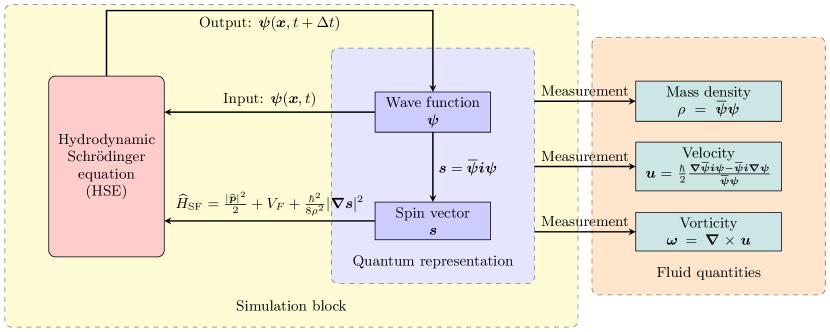
Figure 1: Schematic for quantum computing of the SF.

II.3 Incompressible Schrödinger flow

We consider a special SF for a constant-density incompressible flow with

$$\rho=\rho_{0}.$$ (20)

The wave function on the sphere $\mathbb{S}^{3}$ with radius $\sqrt{\rho_{0}}$ and the spin vector in Eq. (15) on $\mathbb{S}^{2}$ with radius $\rho_{0}$ for this flow are linked by the Hopf fibration [78]. Taking the material derivative $\mathrm{D}/\mathrm{D}t\equiv\partial/\partial t+\boldsymbol{u}\cdot\boldsymbol{\nabla}$ of $\rho$ yields

$$\frac{\mathrm{D}\rho}{\mathrm{D}t}=\frac{\mathrm{D}\mskip 1.5mu\overline{\mskip-1.5mu{\boldsymbol{\psi}}\mskip-1.5mu}\mskip 1.5mu}{\mathrm{D}t}\boldsymbol{\psi}+\mskip 1.5mu\overline{\mskip-1.5mu{\boldsymbol{\psi}}\mskip-1.5mu}\mskip 1.5mu\frac{\mathrm{D}\boldsymbol{\psi}}{\mathrm{D}t}=2\mathrm{Re}\left[\frac{\mathrm{D}\boldsymbol{\psi}}{\mathrm{D}t}\mskip 1.5mu\overline{\mskip-1.5mu{\boldsymbol{\psi}}\mskip-1.5mu}\mskip 1.5mu\right]=0.$$ (21)

Setting $(\mathrm{D}\boldsymbol{\psi}/\mathrm{D}t)\mskip 1.5mu\overline{\mskip-1.5mu{\boldsymbol{\psi}}\mskip-1.5mu}\mskip 1.5mu=\boldsymbol{f}^{\psi}$ as an pure quaternion in Eq. (21) yields

$$\frac{\mathrm{D}\boldsymbol{\psi}}{\mathrm{D}t}=\frac{1}{\rho_{0}}\boldsymbol{f}^{\psi}\boldsymbol{\psi}.$$ (22)

After some algebra, the momentum equation

$$\frac{\partial\boldsymbol{u}}{\partial t}+\boldsymbol{u}\cdot\boldsymbol{\nabla}\boldsymbol{u}=-\boldsymbol{\nabla}\left(\frac{|\boldsymbol{u}|^{2}}{2}-\frac{\hbar}{\rho_{0}^{3}}\boldsymbol{s}\cdot\boldsymbol{f}^{s}\right)-\frac{\hbar}{\rho_{0}^{3}}\boldsymbol{\nabla}\boldsymbol{s}\cdot\boldsymbol{f}^{s}$$ (23)

in an incompressible flow is obtained, where $\boldsymbol{f}^{s}\equiv\mskip 1.5mu\overline{\mskip-1.5mu{\boldsymbol{\psi}}\mskip-1.5mu}\mskip 1.5mu\boldsymbol{f}^{\psi}\boldsymbol{\psi}$ is also a pure quaternion. Note that the flow governed by Eqs. (20) and (23) has some physically interesting properties, such as the helicity conservation [79, 80, 81] and the Lagrangian-like evolution of vortex surfaces [82, 83].

Letting

$$\boldsymbol{f}^{\psi}=-\frac{\boldsymbol{i}}{\hbar}\left(\frac{p}{\rho_{0}}-\frac{|\boldsymbol{u}|^{2}}{2}+V_{F}\right)$$ (24)

and substituting it into Eqs. (22) and (23), we obtain the Euler equation

$$\frac{\partial\boldsymbol{u}}{\partial t}+\boldsymbol{u}\cdot\boldsymbol{\nabla}\boldsymbol{u}=-\boldsymbol{\nabla}\left(\frac{p}{\rho_{0}}+V_{F}\right)$$ (25)

and the corresponding nonlinear Schrödinger equation

$$\boldsymbol{i}\hbar\frac{\partial\boldsymbol{\psi}}{\partial t}=\left(-\frac{{\hbar}^{2}}{2}\nabla^{2}+\frac{p}{\rho_{0}}+V_{F}+\frac{5{\hbar}^{2}}{8\rho_{0}^{2}}|\boldsymbol{\nabla}\boldsymbol{s}|^{2}-\frac{{\hbar}^{2}}{4\rho_{0}^{2}}\boldsymbol{\psi}(\nabla^{2}\boldsymbol{s})\mskip 1.5mu\overline{\mskip-1.5mu{\boldsymbol{\psi}}\mskip-1.5mu}\mskip 1.5mu\boldsymbol{i}\right)\boldsymbol{\psi}.$$ (26)

However, the non-Hermitian Hamiltonian

$$\widehat{H}_{\mathrm{Euler}}=\frac{|\widehat{\boldsymbol{p}}|^{2}}{2}+\frac{p}{\rho_{0}}+V_{F}+\frac{5{\hbar}^{2}}{8\rho_{0}^{2}}|\boldsymbol{\nabla}\boldsymbol{s}|^{2}-\frac{{\hbar}^{2}}{4\rho_{0}^{2}}\boldsymbol{\psi}(\nabla^{2}\boldsymbol{s})\mskip 1.5mu\overline{\mskip-1.5mu{\boldsymbol{\psi}}\mskip-1.5mu}\mskip 1.5mu\boldsymbol{i}$$ (27)

in Eq. (26) can inhibit an efficient quantum computation.

To make the Hamiltonian Hermitian, Eq. (24) is modified to

$$\boldsymbol{f}^{\psi}=-\frac{\boldsymbol{i}}{\hbar}\left(\frac{p}{\rho_{0}}-\frac{|\boldsymbol{u}|^{2}}{2}+V_{F}\right)-\frac{\hbar}{4\rho_{0}^{3}}\boldsymbol{\psi s}(\boldsymbol{s}\times\nabla^{2}\boldsymbol{s})\mskip 1.5mu\overline{\mskip-1.5mu{\boldsymbol{\psi}}\mskip-1.5mu}\mskip 1.5mu.$$ (28)

Then we have the modified momentum equation

$$\frac{\partial\boldsymbol{u}}{\partial t}+\boldsymbol{u}\cdot\boldsymbol{\nabla}\boldsymbol{u}=-\boldsymbol{\nabla}\left(\frac{p}{\rho_{0}}+V_{F}\right)-\frac{\hbar^{2}}{4\rho_{0}^{2}}\boldsymbol{\nabla}\boldsymbol{s}\cdot\nabla^{2}\boldsymbol{s},$$ (29)

and the incompressible hydrodynamic Schrödinger equation (IHSE)

$$\boldsymbol{i}\hbar\frac{\partial\boldsymbol{\psi}}{\partial t}=\left(-\frac{{\hbar}^{2}}{2}\nabla^{2}+\frac{p}{\rho_{0}}+V_{F}(\boldsymbol{x})-\frac{{\hbar}^{2}}{8\rho_{0}^{2}}|\boldsymbol{\nabla}\boldsymbol{s}|^{2}\right)\boldsymbol{\psi}.$$ (30)

The physical meaning of the last term in the RHS of Eq. (29), i.e., the LLF [74, 75], is further discussed in Appendix B. The flow governed by Eq. (29) with $\rho_{0}=1$ has been called the incompressible Schrödinger flow (ISF) [74, 75] and studied by numerical simulations [84]. The Hamiltonian of the ISF

$$\widehat{H}_{\mathrm{ISF}}=\frac{|\widehat{\boldsymbol{p}}|^{2}}{2}+\frac{p}{\rho_{0}}+V_{F}-\frac{\hbar^{2}}{8\rho_{0}^{2}}|\boldsymbol{\nabla}\boldsymbol{s}|^{2}$$ (31)

is Hermitian, so the ISF is suitable for quantum computing. Moreover, the form of the IHSE can be obtained by setting $\rho=\rho_{0}$ in the HSE.

Similar to the incompressible Navier–Stokes equation (INSE), the pressure $p$ in the IHSE (30) is coupled with Eq. (29) to ensure the divergence-free velocity. Thus, the mathematical natures of the HSE (16) with non-constant $\rho$ and IHSE (30) are very different, which is similar to the difference between compressible and incompressible NSEs, so they have to be solved by different methods. In the present study, we focus on the physical property and quantum algorithm for the ISF.

III Turbulent ISFs

We investigate two ISFs, the Taylor–Green (TG) flow and decaying homogeneous isotropic turbulence (HIT), to illustrate the similarities and differences between the ISF and the real viscous flow. Additionally, the evolution of vortex knots was investigated in the ISF [84].

Since quantum hardware and algorithms for simulating such complex flows are still under development, the DNS of the ISF was carried out to solve Eq. (30) with $\rho_{0}=1$ on a classical computer. The standard pseudo-spectral method [85, 83, 86] was adopted in a periodic cube of side $\mathcal{L}=2\pi$ on $512^{3}$ uniform grid points. The numerical implementation was described in detail in Ref. [84].

III.1 TG flow

We apply the TG initial condition in Eq. (79) to the INSE and IHSE. The construction of the initial wave function is detailed in Appendix C. The evolutions of the TG vortex in the ISF and the incompressible NS flow (INSF) are compared in Fig. 2 using the contour of the vorticity magnitude $|\boldsymbol{\omega}|$ with $\boldsymbol{\omega}\equiv\boldsymbol{\nabla}\times\boldsymbol{u}$. In the INSF, the initial blob-like vortices are stretched into sheet-like structures and move towards symmetry planes at $t=4$. In the ISF, the vortices undergo strongly oscillating shearing motion, and they break up into smaller-scale vortices at $t=1$. The characteristic time scale of vortex dynamics in the ISF is much smaller than that in the INSF.

\begin{overpic}[width=433.62pt]{fig2.png} \small \put(0.0,35.4){(a)} \put(4.5,35.4){$t=0.0$} \put(21.5,35.4){$t=2.0$} \put(38.3,35.4){$t=3.0$} \put(55.2,35.4){$t=4.0$} \put(72.0,35.4){$t=6.0$} \put(89.1,35.4){$t=8.0$} \put(0.0,16.25){(b)} \put(4.5,16.25){$t=0.0$} \put(21.5,16.25){$t=0.1$} \put(38.3,16.25){$t=0.2$} \put(55.2,16.25){$t=0.5$} \put(72.0,16.25){$t=0.8$} \put(89.1,16.25){$t=1.0$} \end{overpic}

Figure 2: Evolution of $|\boldsymbol{\omega}|$ on the $x$–$y$ plane at $z=\pi$ for TG vortices in the (a) INSF with $\mathit{Re}=1000$ and (b) ISF with $\hbar=1$. The contour is color-coded by $0\leqslant|\boldsymbol{\omega}|/|\boldsymbol{\omega}|_{\max}\leqslant 1$ from blue to red.

The effect of the parameter $\hbar$ in the ISF is similar to the kinetic viscosity $\nu$ in the INSF. Figure 3 shows similar large-scale vortical structures with $\hbar=1$ and 0.1, whereas much more small-scale tube-like structures emerge for smaller $\hbar=0.1$. In general, the length scale of vortices is proportional to $\hbar$ via the vorticity Clebsch mapping [74, 75, 84], and the flow stability depends on the value of $\hbar$. In Fig. 3, the flow with smooth large-scale structures does not have a transition for $\hbar=1$, whereas the flow breaks down into turbulence with numerous chaotic vortex tubes for $\hbar=0.1$. The energy spectrum $E_{k}(k)$ of a turbulent ISF in Fig. 4 exhibits a $-5/3$ scaling law in the inertial range as in classical turbulence [29]. As $\hbar$ decreases, the inertial range broadens with a more pronounced $-5/3$ scaling.

\begin{overpic}[width=433.62pt]{fig3.png} \small \put(0.0,41.0){(a)} \put(48.0,41.0){(b)} \footnotesize \put(93.6,44.0){$|\boldsymbol{\omega}|$} \put(96.5,0.4){$0$} \put(96.5,10.9){$2.5$} \put(96.5,21.4){$5$} \put(96.5,32.0){$7.5$} \put(96.5,42.4){$10$} \end{overpic}

Figure 3: Isosurfaces of $s_{1}=-0.9$ at $t=1$ for TG vortices in the ISF with (a) $\hbar=1$ and (b) $\hbar=0.1$. Note that the isosurface of $s_{1}$ is a vortex surface [82, 83] consisting of vortex lines, and the initial isosurface is a vortex column shown in Fig. 15(a). The isosurfaces are color-coded by $|\boldsymbol{\omega}|$.

\begin{overpic}[width=173.44534pt]{fig4a.pdf} \small \put(0.0,3.0){$10^{0}$} \put(42.0,3.0){$10^{1}$} \put(83.6,3.0){$10^{2}$} \put(50.0,-4.0){$k$} \put(-13.0,7.8){$10^{-15}$} \put(-13.0,16.8){$10^{-13}$} \put(-13.0,26.2){$10^{-11}$} \put(-10.6,35.5){$10^{-9}$} \put(-10.6,44.9){$10^{-7}$} \put(-10.6,54.2){$10^{-5}$} \put(-10.6,63.5){$10^{-3}$} \put(-10.6,72.7){$10^{-1}$} \put(-20.0,44.0){$E_{k}$} \put(-20.0,76.0){(a)} \footnotesize \put(52.0,21.0){$t$} \put(60.0,66.0){\begin{rotate}{-10.0} $k^{-5/3}$ \end{rotate}} \end{overpic}

\begin{overpic}[width=173.44534pt]{fig4b.pdf} \small \put(0.0,3.0){$10^{0}$} \put(42.0,3.0){$10^{1}$} \put(83.6,3.0){$10^{2}$} \put(50.0,-4.0){$k$} \put(-13.0,7.8){$10^{-15}$} \put(-13.0,16.8){$10^{-13}$} \put(-13.0,26.2){$10^{-11}$} \put(-10.6,35.5){$10^{-9}$} \put(-10.6,44.9){$10^{-7}$} \put(-10.6,54.2){$10^{-5}$} \put(-10.6,63.5){$10^{-3}$} \put(-10.6,72.7){$10^{-1}$} \put(-20.0,44.0){$E_{k}$} \put(-20.0,76.0){(b)} \footnotesize \put(20.0,61.0){$t$} \put(60.0,68.0){\begin{rotate}{-10.0} $k^{-5/3}$ \end{rotate}} \end{overpic}

Figure 4: Evolution of the energy spectra for TG vortices in the ISF at $t=1\sim 8$ with (a) $\hbar=1$ and (b) $\hbar=0.1$.

III.2 Decaying HIT

We construct an initial $\boldsymbol{\psi}(\boldsymbol{x},t=0)$, corresponding to a random divergence-free velocity, for simulating HIT in the ISF. First, a normalized Gaussian-random wave function

$$\begin{split}\boldsymbol{\psi}^{*}=\ &\frac{1}{\sqrt{-2\ln(r_{1}r_{3})}}\left(\sqrt{-2\ln r_{1}}\cos(2\pi r_{2})+\sqrt{-2\ln r_{1}}\sin(2\pi r_{2})\boldsymbol{i}\right.\\ &+\left.\sqrt{-2\ln r_{3}}\cos(2\pi r_{4})\boldsymbol{j}+\sqrt{-2\ln r_{3}}\sin(2\pi r_{4})\boldsymbol{k}\right)\end{split}$$ (32)

was generated, where $r_{1}$, $r_{2}$, $r_{3}$, and $r_{4}$ are independently generated real random numbers satisfying the uniform distribution within $[0,1]$. Second, a divergence-free projection $\boldsymbol{\psi}^{**}=\mathrm{e}^{-\mathrm{i}q/\hbar}\boldsymbol{\psi}^{*}$ was applied, where $q$ is solved from $\nabla^{2}q=\hbar(\nabla^{2}\mskip 1.5mu\overline{\mskip-1.5mu{\boldsymbol{\psi}^{*}}\mskip-1.5mu}\mskip 1.5mu\boldsymbol{i}\boldsymbol{\psi}^{*}-\mskip 1.5mu\overline{\mskip-1.5mu{\boldsymbol{\psi}^{*}}\mskip-1.5mu}\mskip 1.5mu\boldsymbol{i}\nabla^{2}\boldsymbol{{\psi}}^{*})/2$. Third, $\boldsymbol{\psi}^{**}$ was evolved using the IHSE for a time period $t_{0}=5$ to smooth the noisy initial $\boldsymbol{\psi}^{**}$. Finally, $\boldsymbol{\psi}(\boldsymbol{x},t=0)=\boldsymbol{\psi}^{**}(\boldsymbol{x},t_{0}=5)$ and its corresponding velocity were taken as the initial conditions of IHSE and INSE, respectively.

The vortex surface [82] in the fully developed turbulent ISF at $t=5$ is visualized in Fig. 5 using the isosurface of $s_{1}s_{2}s_{3}=0.18$. We observe a network of entangled vortex tubes and sheets, which can be mapped to closed curves, the intersection of $s_{1}^{2}+s_{2}^{2}+s_{3}^{2}=1$ and $s_{1}s_{2}s_{3}=0.18$, on the unit sphere $\mathbb{S}^{2}$ (or the Bloch sphere) via the vorticity Clebsch mapping [74, 75, 84]. The geometry of vortex surfaces in the ISF is in between the vortex filaments in quantum turbulence [87, 88, 89] and the tangle of spiral vortex tubes and sheets in classical turbulence [90, 91, 85]. Therefore, the turbulent ISF manifests the features of both quantum and classical turbulent flows.

\begin{overpic}[width=433.62pt]{fig5.png} \small \put(0.0,45.0){(a)} \put(52.0,45.0){(b)} \footnotesize \put(92.8,46.0){$|\boldsymbol{\omega}|$} \put(96.0,3.2){$0$} \put(96.0,13.375){$1.25$} \put(96.0,23.55){$2.5$} \put(96.0,33.725){$3.75$} \put(96.0,43.9){$5$} \end{overpic}

Figure 5: Visualization of the tangled vortex tubes for the decaying HIT in the ISF. (a) Isosurface of $s_{1}s_{2}s_{3}=0.18$ color-coded by $|\boldsymbol{\omega}|$ at $t=5$. (b) Close-up view of the region marked by the blue box in (a). Some vortex lines (blue) are integrated and plotted on the isosurface in (b).

Figure 6 shows the evolution of $E_{k}(k)$ for the decaying HIT in the ISF with $\hbar=0.1$ and the INSF with $\nu=0.0005$ (or $\mathit{Re}=2000$ for unity length and velocity scales). The energy spectrum in the ISF exhibits the $-5/3$ scaling law in the inertial range as in classical turbulence [29], and it decays with time due to energy dissipation. In addition, the total kinetic energy decays with time in the turbulent ISF as in the classical HIT (not shown).

\begin{overpic}[width=173.44534pt]{fig6.pdf} \small \put(0.0,3.0){$10^{0}$} \put(47.0,3.0){$10^{1}$} \put(93.0,3.0){$10^{2}$} \put(50.0,-4.0){$k$} \put(-10.6,11.0){$10^{-8}$} \put(-10.6,22.2){$10^{-7}$} \put(-10.6,33.3){$10^{-6}$} \put(-10.6,44.2){$10^{-5}$} \put(-10.6,55.4){$10^{-4}$} \put(-10.6,66.5){$10^{-3}$} \put(-10.6,77.6){$10^{-2}$} \put(-20.0,44.0){$E_{k}$} \footnotesize \put(30.0,45.0){$t=0$} \put(30.0,38.0){$t=5$, ISF} \put(30.0,31.0){$t=10$, ISF} \put(30.0,24.0){$t=5$, INSF} \put(30.0,17.0){$t=10$, INSF} \put(80.0,60.0){\begin{rotate}{-15.0} $k^{-5/3}$ \end{rotate}} \end{overpic}

Figure 6: Evolution of the energy spectra for the decaying HIT in the ISF with $\hbar=0.1$ and the INSF with $\mathit{Re}=2000$.

IV Quantum algorithm for the ISF

IV.1 Prediction-correction approach

We develop a quantum algorithm for simulating the ISF. As sketched in Fig. 1, the algorithm can be executed on a quantum processor with measurements only at the end of the simulation, so it does not involve frequent information exchanges between classical and quantum hardware as in existing hybrid quantum-classical methods [92, 43, 46, 45]. This quantum algorithm can have significant advantages over classical and hybrid ones in terms of computational speedup, memory saving, and reduction of noises introduced by measurements.

We apply a prediction-correction approach to bypass handling the nonlinear potential in Eq. (14) in the IHSE. As in classical algorithms [93, 94, 95] for simulating incompressible flows, the pressure is not solved using the pressure-Poisson equation

$$\nabla^{2}p=\boldsymbol{\nabla}\cdot\left(\boldsymbol{u}\times\boldsymbol{\omega}-\frac{\hbar^{2}}{4}\boldsymbol{\nabla}\boldsymbol{s}\cdot\nabla^{2}\boldsymbol{s}\right)-\nabla^{2}\left(V_{F}+\frac{|\boldsymbol{u}|^{2}}{2}\right),$$ (33)

because the RHS in Eq. (33) is difficult to encode on a quantum computer. First, we perform a prediction to obtain a temporary wave function using Eq. (30) with ignoring $p-\hbar^{2}|\boldsymbol{\nabla}\boldsymbol{s}|^{2}/8$. Second, we apply a divergence-free projection of the temporary wave function. The flowchart of this quantum algorithm the ISF is illustrated in Fig. 7. Next, we elaborate each step in the algorithm in Fig. 7 using a 1D problem, and it is straightforward to extend the algorithm to 3D problems.

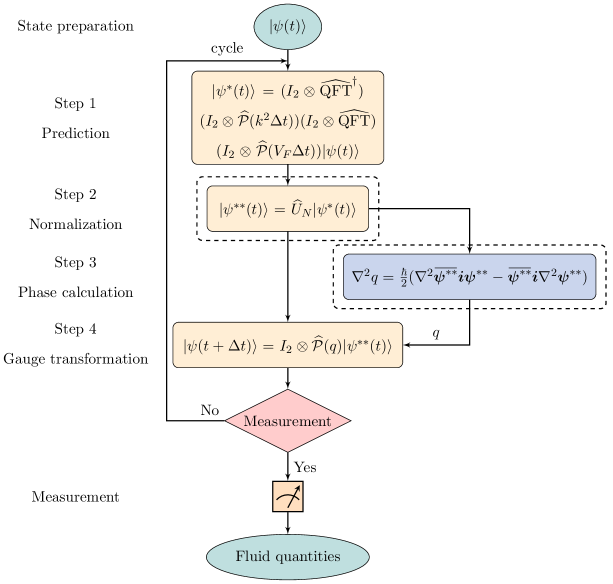
Figure 7: Flowchart of the quantum algorithm for simulating the ISF. The dashed boxes highlight the bottlenecks of quantum speedup in the present algorithm.

IV.2 Quantum encoding of the IHSE

In an $n+1$-qubit quantum register, the state of a “Pauli particle” [71, 72, 73], whose motion is governed by the IHSE (30) with $\rho=1$, can be encoded as follows. We use $n$ qubits with state vectors $|j_{0}\rangle,|j_{1}\rangle,\cdots,|j_{n-1}\rangle$ to encode a particle location. The last qubit $|j_{n}\rangle=|s\rangle$ stores the spin state of the particle. The state of each qubit $j_{0},j_{1},\cdots,j_{n-1},j_{n}$ takes the value 0 or 1. The domain $-d\leqslant x\leqslant d$ for the particle location is discretized into $2^{n}$ segments with the spacing $\Delta x=2d/2^{n}$. These segments can be represented by the computational basis $|x_{j}\rangle=|j_{n-1}j_{n-2}\cdots j_{0}\rangle$ in the Hilbert space $\mathbb{C}^{2^{n}}$ with the shorthand $|j_{n-1}j_{n-2}\cdots j_{0}\rangle\equiv|j_{n-1}\rangle\otimes|j_{n-2}\rangle\otimes\cdots\otimes|j_{0}\rangle$.

In this way, the quaternionic wave function $\boldsymbol{\psi}(x,t)$ is approximated by the state vector

$$|\psi\rangle=\frac{1}{\mathcal{N}}\sum_{s=0}^{1}\sum_{j_{n-1}=0}^{1}\cdots\sum_{j_{0}=0}^{1}\psi_{s}(x_{j},t)|s\rangle\otimes|j_{n-1}j_{n-2}\cdots j_{0}\rangle$$ (34)

with $\psi_{0}\equiv a+\mathrm{i}b$, $\psi_{1}\equiv c+\mathrm{i}d$, $x_{j}\equiv-d+(j+\frac{1}{2})\Delta x$, $j=\sum_{i=0}^{n-1}j_{i}2^{i}$, and

$$\mathcal{N}=\sqrt{\sum_{s=0}^{1}\sum_{j=0}^{2^{n}-1}|\psi_{s}(x_{j},t)|^{2}}=\sqrt{2^{n}\rho}=\sqrt{2^{n}}.$$ (35)

Hence, the wave function is reconstructed by

$$\boldsymbol{\psi}(x_{j},t)=\sqrt{2^{n}}\left(\mathrm{Re}{\langle x_{j}0\,|\,\psi\rangle}+\mathrm{Im}{\langle x_{j}0\,|\,\psi\rangle}\boldsymbol{i}+\mathrm{Re}{\langle x_{j}1\,|\,\psi\rangle}\boldsymbol{j}+\mathrm{Im}{\langle x_{j}1\,|\,\psi\rangle}\boldsymbol{k}\right).$$ (36)

IV.3 Quantum algorithm for solving the IHSE

Step 1: Prediction

In step 1, we treat the particle governed by the IHSE as a free Pauli particle. Namely, Eq. (30) becomes $\boldsymbol{i}\hbar\frac{\partial}{\partial t}\boldsymbol{\psi}(x,t)=\left(-\frac{\hbar^{2}}{2}\partial_{x}^{2}+V_{F}(x)\right)\boldsymbol{\psi}(x,t)$. The motion of such a particle is described by a temporary solution [96, 19, 97, 98]

$$|\psi^{*}(t)\rangle=\left(I_{2}\otimes\widehat{\mathrm{QFT}}^{\dagger}\right)\left(I_{2}\otimes\widehat{\mathcal{P}}(k^{2}\Delta t)\right)\left(I_{2}\otimes\widehat{\mathrm{QFT}}\right)\left(I_{2}\otimes\widehat{\mathcal{P}}(V_{F}\Delta t)\right)|\psi(t)\rangle$$ (37)

with the $2^{1}\times 2^{1}$ identity matrix $I_{2}$, the quantum Fourier transform (QFT) [99, 100, 101]

$$\widehat{\mathrm{QFT}}:~{}|j\rangle\to\frac{1}{\sqrt{2^{n}}}\sum_{k=0}^{2^{n}-1}\mathrm{e}^{2\pi\mathrm{i}\frac{jk}{2^{n}}}|k\rangle,$$ (38)

the Hermitian transpose ${\dagger}$, and the diagonal unitary transformation $\widehat{\mathcal{P}}(f)\equiv\mathrm{e}^{-\mathrm{i}f/\hbar}$. The QFT can be implemented by $\mathcal{O}(n^{2})$ quantum gates in Fig. 8, which achieves an exponential acceleration compared to $\mathcal{O}(n2^{n})$ operations of the fast Fourier transform. Equation (37) is an approximation based on the second-order Trotter decomposition [2]

$$\mathrm{e}^{-\mathrm{i}(H_{0}+V_{F})\Delta t/\hbar}=\mathrm{e}^{-\mathrm{i}H_{0}\Delta t/\hbar}\mathrm{e}^{-\mathrm{i}V_{F}(x)\Delta t/\hbar}+\mathcal{O}(\Delta t^{2}),$$ (39)

because the kinetic energy $H_{0}=|\widehat{\boldsymbol{p}}|^{2}/2$ and $V_{F}$ are not commute, i.e., $[H_{0},V_{F}]\neq 0$. The time stepping $\Delta t$ should be small enough to ensure accuracy.

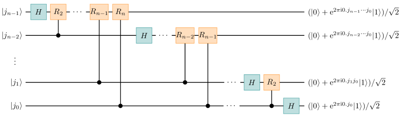
Figure 8: Quantum circuit for the QFT in Eq. (38) with $n$ qubits, where the SWAP gates for reversing the order of qubits in the end of the QFT are not shown.

An efficient quantum implementation of $\widehat{\mathcal{P}}(f)$ in Eq. (37) is important. The variable

$$x_{j}=-d+\left(j+\frac{1}{2}\right)\Delta x=c_{0}\sum_{i=0}^{n-1}\left(j_{i}2^{i}+c_{1}\right)$$ (40)

in $V(x)$ is discretized with constants $c_{0}=\Delta x$ and $c_{1}=(-d+\Delta x/2)/(n\Delta x)$, and thus

$$\widehat{\mathcal{P}}(V_{F}\Delta t):~{}|j\rangle\to\mathrm{e}^{-\mathrm{i}V_{F}\left(c_{0}\sum_{i=0}^{n-1}(j_{i}2^{i}+c_{1})\right)\Delta t/\hbar}|j\rangle$$ (41)

is computable.

Similarly, we express the $n$-bit number $k=\sum_{j=0}^{n-1}k_{j}2^{j}$ with $k_{0},k_{1},\cdots,k_{n-1}\in\{0,1\}$ in the momentum operator $\widehat{\mathcal{P}}(k^{2}\Delta t)$ in Eq. (37). Using the wavenumber expressed by [96, 102]

$$k=\sqrt{\frac{1}{2^{2n-3}}\frac{\phi\hbar}{\Delta t}}\left(1+\sum_{j=0}^{n-1}2^{j}\widehat{Z}_{j}\right),$$ (42)

we obtain

$$\widehat{\mathcal{P}}(k^{2}\Delta t)=\exp\left(\frac{\mathrm{i}\phi}{2^{2n-3}}\right)\prod_{\ell=0}^{n-1}\exp\left(\frac{\mathrm{i}\phi}{2^{2n-\ell-4}}\widehat{Z}_{\ell}\right)\prod_{\begin{subarray}{c}i,j=0\\ i>j\end{subarray}}^{n-1}\exp\left(\frac{\mathrm{i}\phi}{2^{2n-i-j}}\widehat{Z}_{i}\otimes\widehat{Z}_{j}\right).$$ (43)

Here, $\widehat{Z}_{j}$ denotes a phase-shift gate at the $j$-th qubit and $\phi=\Delta t/\hbar$ is a small phase shift on a time step. The quantum circuit for calculating a Hamiltonian with the form of $\widehat{H}=\exp(\mathrm{i}\Delta t\widehat{Z}_{2}\otimes\widehat{Z}_{1}\otimes\widehat{Z}_{0})$ with a given $\Delta t$ is shown in Fig. 9, using an ancilla qubit [2]. Taking, e.g., $n=3$ qubits and ignoring the global phase $\mathrm{e}^{\mathrm{i}\phi/8}$, Eq. (43) becomes

$$\widehat{P}(k^{2}\Delta t)=\exp\left[\mathrm{i}\phi\left(\widehat{Z}_{2}+\frac{1}{2}\widehat{Z}_{1}+\frac{1}{4}\widehat{Z}_{0}+2\widehat{Z}_{2}\otimes\widehat{Z}_{1}+\widehat{Z}_{2}\otimes\widehat{Z}_{0}+\frac{1}{2}\widehat{Z}_{1}\otimes\widehat{Z}_{0}\right)\right],$$ (44)

which can be realized by a quantum circuit in Fig. 10. Thus, only $\mathcal{O}(n^{2})$ quantum gates are sufficient to calculate the momentum operator in Eq. (43).

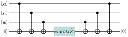
Figure 9: Quantum circuit for calculating $\widehat{H}=\exp(\mathrm{i}\Delta t\widehat{Z})$ with an ancilla qubit and $\widehat{Z}=\widehat{Z}_{2}\otimes\widehat{Z}_{1}\otimes\widehat{Z}_{0}$.

Figure 10: Quantum circuit for calculating $\widehat{\mathcal{P}}(k^{2}\Delta t)$ in Eq. (44) with $n=3$ qubits and an ancilla qubit.

Step 2: Normalization

Since the temporary solution $\boldsymbol{\psi}^{*}(x,t)$ obtained from Eq. (37) in step 1 is not necessarily on $\mathbb{S}^{3}$, i.e., $\mskip 1.5mu\overline{\mskip-1.5mu{\boldsymbol{\psi}^{*}}\mskip-1.5mu}\mskip 1.5mu\boldsymbol{\psi}^{*}\neq 1$, it is normalized as

$$|\psi^{**}(t)\rangle=\widehat{U}_{N}|\psi^{*}(t)\rangle$$ (45)

in step 2, with an unitary operation $\widehat{U}_{N}$ to obtain $\mskip 1.5mu\overline{\mskip-1.5mu{\boldsymbol{\psi}^{**}}\mskip-1.5mu}\mskip 1.5mu\boldsymbol{\psi}^{**}=1$.

This normalization step appears to be difficult to implement on a quantum computer. As illustrated in Fig. 11, we can only conceptually decompose the operator

$$\widehat{U}_{N}=Q_{2^{n}-1}Q_{2^{n}-2}\cdots Q_{1}Q_{0}=\prod_{i=0}^{2^{n}-1}Q_{2^{n}-1-i},$$ (46)

with scale transformations

$$Q_{i}:~{}\frac{1}{\sqrt{2^{n}}}\sum_{s=0}^{1}\sum_{j=0}^{2^{n}-1}\psi_{s}(x_{j},t)|s\rangle\otimes|j\rangle\to\frac{1}{\sqrt{2^{n}}}\sum_{s=0}^{1}\sum_{j=0}^{2^{n}-1}\frac{\psi_{s}(x_{j},t)}{\sqrt{|\psi_{0}(x_{j},t)|^{2}+|\psi_{1}(x_{j},t)|^{2}}}|s\rangle\otimes|j\rangle.$$ (47)

Here, each $Q_{i}$ may be non-unitary with $Q_{i}^{\dagger}Q_{i}\neq I$ and thus it is not realizable using a quantum gate, whereas their product Eq. (46) is unitary. Therefore, an effective quantum algorithm for calculating $\widehat{U}_{N}$ with the complexity $\mathcal{O}(\mathrm{poly}(n))$ remains an open problem.

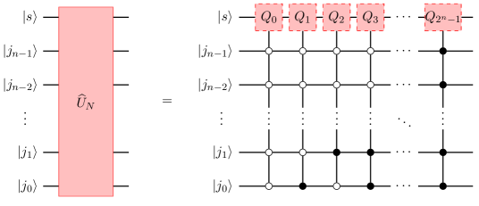
Figure 11: Conceptual quantum circuit for calculating $\widehat{U}_{N}$ in Eq. (46). The dashed boxes mark that $Q_{i},~{}i=1,2,\cdots,2^{n}-1$ may be non-unitary, so they are not realizable quantum gates. Hollow and solid circles denote control qubits with values 0 and 1, respectively. The operation $Q_{j}$ on the target qubit $|s\rangle$ is active only when the control qubits are in the state $|j\rangle=|j_{n-1}j_{n-2}\cdots j_{0}\rangle$ with $j=\sum_{i=0}^{n-1}j_{i}2^{i}$.

Step 3: Phase calculation

After step 2, the divergence of the velocity $u^{**}=\hbar(\partial_{x}\mskip 1.5mu\overline{\mskip-1.5mu{\boldsymbol{\psi}^{**}}\mskip-1.5mu}\mskip 1.5mu\boldsymbol{i}\boldsymbol{\psi}^{**}-\mskip 1.5mu\overline{\mskip-1.5mu{\boldsymbol{\psi}^{**}}\mskip-1.5mu}\mskip 1.5mu\boldsymbol{i}\partial_{x}\boldsymbol{\psi}^{**})/2$ can be non-zero. A divergence-free projection of $u^{**}$, as a gauge transformation $\boldsymbol{u}\to\boldsymbol{u}-\boldsymbol{\nabla}q$, is applied, where the phase $q$ is solved from a Poisson equation

$$\partial_{x}^{2}q=\frac{\hbar}{2}\left(\partial_{x}^{2}\mskip 1.5mu\overline{\mskip-1.5mu{\boldsymbol{\psi}^{**}}\mskip-1.5mu}\mskip 1.5mu\boldsymbol{i}\boldsymbol{\psi}^{**}-\mskip 1.5mu\overline{\mskip-1.5mu{\boldsymbol{\psi}^{**}}\mskip-1.5mu}\mskip 1.5mu\boldsymbol{i}\partial_{x}^{2}\boldsymbol{{\psi}}^{**}\right).$$ (48)

This projection corresponds to the gauge transformation $\boldsymbol{\psi}\to\mathrm{e}^{-\mathrm{i}q/\hbar}\boldsymbol{\psi}$ for the wave function [103].

The encoding of the RHS of Eq. (48) without affecting the quantum state $|\psi^{**}\rangle$ appears to be challenging. A solution of this issue admits an efficient quantum algorithm [34, 104, 105, 106, 107] to solve Eq. (48) using $\mathcal{O}(\mathrm{poly}(n))$ basic quantum gates.

Step 4: Gauge transformation

In the final step, we take a gauge transformation

$$|\psi(t+\Delta t)\rangle=I_{2}\otimes\widehat{\mathcal{P}}(q)|\psi^{**}(t)\rangle$$ (49)

from the temporary state $|\psi^{**}\rangle$ at $t$ to the state $|\psi\rangle$ at $t+\Delta t$. The diagonal unitary transformation

$$\widehat{\mathcal{P}}(f(x)):\quad|x\rangle\to\mathrm{e}^{-\mathrm{i}f(x)/\hbar}|x\rangle$$ (50)

of a function $f(x)$ can be implemented by $\mathcal{O}(2^{n})$ generalized controlled-phase shift gates. They apply the single qubit gate $F_{j}$ to a target qubit $|j_{0}\rangle$ only when the other $n-1$ controlled qubits are in the state $|j\rangle=|j_{n-1}j_{n-2}\cdots j_{1}\rangle$ [96]. An example with $n=4$ qubits is shown in Fig. 12.

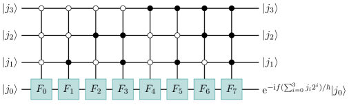
Figure 12: Quantum circuit for calculating $\widehat{\mathcal{P}}(f(x))$ in Eq. (50) with $n=4$ qubits. Hollow and solid circles denote control qubits with values 0 and 1, respectively. The operation $F_{j}$ on the target qubit $|j_{0}\rangle$ is active only when the control qubits are in the state $|j\rangle=|j_{3}j_{2}j_{1}\rangle$ with $j=\sum_{i=0}^{2}j_{i+1}2^{i}$.

However, such an implementation is inefficient because its complexity scales exponentially with $n$. A more efficient quantum circuit can be designed for a specific form of $f(x)$, e.g., only $\mathcal{O}(n^{2})$ basic quantum gates are used for $f(k)=k^{2}\Delta t$ in Eq. (37). In general, if $f(x)$ has a specific form, e.g., $f(x)$ for the harmonic oscillator, square well, and quantum tunneling, Eq. (50) can be calculated with the complexity $\mathcal{O}(\mathrm{poly}(n))$.

Algorithm complexity

We estimate the total complexity of the quantum algorithm for solving the IHSE in Eq. (30). The overall quantum circuit with the prediction, normalization, phase calculation, and gauge transformation is illustrated in Fig. 13. The prediction is a standard simulation of a potential-free Pauli particle, using only $\mathcal{O}(n^{2})$ basic quantum gates. The normalization is unconventional in quantum computing. The upper and lower bounds of operations are $\mathcal{O}(2^{n})$ and $\mathcal{O}(\mathrm{poly}(n))$, respectively. The gauge transformation, currently, can only be realized through the generic diagonal unitary transformation in Fig. 12, using $\mathcal{O}(2^{n})$ basic quantum gates.

The complexities of each step and the entire algorithm are summarized in Table 2. The present quantum algorithm can achieve exponential speedup in steps 1 and 3, and possible

$$S_{1}=\frac{n2^{n}+\mathrm{poly}(2^{n})}{\mathrm{poly}(n)}$$ (51)

speedup overall. The bottlenecks for the computational efficiency in steps 2 and 4 need to be tackled in the future work.

Besides the spatial complexity, the temporal and spatial steps are related by the Courant–Friedrichs–Lewy (CFL) condition in both the quantum and classical implementations. This implies that the number of time iterations is $N_{t}=\mathcal{O}(N)$, where $N=2^{n}$ is the total number of grid points. Thus, the numerical error $\epsilon$ decreases polynomially with the number of grid points. Assuming that the unitary operators are smooth enough and the norm of the exponential operators are bounded by one [108, 109], the error after $N_{t}$ iterations scales as $\epsilon\sim N_{t}\Delta t^{2}\sim N^{-1}$ for the second-order Trotter decomposition. Given an error tolerance, the upper and lower bounds of the number of gates scale as $N_{\mathrm{gate}}\sim\epsilon^{-1}\mathrm{poly}(\log_{2}\epsilon^{-1})$ and $N_{\mathrm{gate}}\sim\epsilon^{-2}$, respectively, for a quantum algorithm. In the classical algorithm, the number of operations scales as $N_{\mathrm{op}}\sim\epsilon^{-1}(\epsilon^{-1}\log_{2}\epsilon^{-1}+\mathrm{poly}(\epsilon^{-1}))$. Therefore, even if the CFL condition constrains the time stepping, the quantum algorithm has a possible exponential speedup

$$S_{2}=\frac{\epsilon^{-1}(\epsilon^{-1}\log_{2}\epsilon^{-1}+\mathrm{poly}(\epsilon^{-1}))}{\epsilon^{-1}\mathrm{poly}(\log_{2}\epsilon^{-1})}=\frac{\epsilon^{-1}\log_{2}\epsilon^{-1}+\mathrm{poly}(\epsilon^{-1})}{\mathrm{poly}(\log_{2}\epsilon^{-1})}.$$ (52)

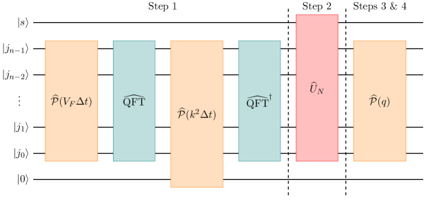
Figure 13: Overall quantum circuit for solving the IHSE, from time $t$ to $t+\Delta t$. The bottom qubit is an auxiliary one for implementing the momentum operator.

Table 2: Breakdown of algorithm complexities of quantum and classical algorithms.

	Step 1	Step 2	Step 3	Step 4	Total
Quantum	$\mathcal{O}(n^{2})$	$\mathcal{O}(\mathrm{poly}(n))$–$\mathcal{O}(2^{n})$	$\mathcal{O}(\mathrm{poly}(n))$	$\mathcal{O}(\mathrm{poly}(n))$–$\mathcal{O}(2^{n})$	$\mathcal{O}(\mathrm{poly}(n))$–$\mathcal{O}(2^{n})$
Classical	$\mathcal{O}(n2^{n})$	$\mathcal{O}(2^{n})$	$\mathcal{O}(\mathrm{poly}(2^{n}))$	$\mathcal{O}(2^{n})$	$\mathcal{O}(n2^{n}+\mathrm{poly}(2^{n}))$

IV.4 Qiskit implementation

We provide a simple 1D example to go through the entire algorithm, which is implemented on a quantum computer with exponential speedup. The initial wave function is

$$\boldsymbol{\psi}(x,t=0)=\frac{\sqrt{2}}{2}\left(\cos\frac{x}{\hbar}+\sin\frac{x}{\hbar}\boldsymbol{i}+\cos\frac{x}{\hbar}\boldsymbol{j}+\sin\frac{x}{\hbar}\boldsymbol{k}\right),$$ (53)

and the corresponding spin vector is $\boldsymbol{s}(x,0)=(0,0,1)$. The solution of this steady ISF satisfies a Helmholtz equation

$$\partial_{x}^{2}\boldsymbol{\psi}-\left(\frac{2}{\hbar^{2}}p-\frac{1}{4}|\partial_{x}\boldsymbol{s}|^{2}\right)\boldsymbol{\psi}=\boldsymbol{0}.$$ (54)

This simplified IHSE with $V_{F}=0$ with the initial condition in Eq. (53) has a steady solution $u=1$, where the nonlinear potential in Eq. (30) is simplified to $p=-1/2$. Thus, we only need to perform steps 1 and 4 as

$$|\psi(t+\Delta t)\rangle=\left(I_{2}\otimes\widehat{\mathcal{P}}(-\frac{\Delta t}{2})\right)\left(I_{2}\otimes\widehat{\mathrm{QFT}}^{\dagger}\right)\left(I_{2}\otimes\widehat{\mathcal{P}}(k^{2}\Delta t)\right)\left(I_{2}\otimes\widehat{\mathrm{QFT}}\right)|\psi(t)\rangle.$$ (55)

The complexity for calculating a time step of Eq. (55) is $\mathcal{O}(n^{2})$. Compared to $\mathcal{O}(\mathrm{poly}(2^{n}n))$ for the classical algorithm, the exponential quantum speedup is achieved.

We validate the algorithm in Eq. (55) using IBM’s Qiskit [57]. The Qiskit is an open-source software development kit for quantum computers at the level of pulses, circuits, and application modules. We used a simulator with the quantum assembly language (QASM) on a classical computer, which mimics a quantum computer by adding small noises to the result [110]. The QASM also operates by running the quantum circuit multiple times and storing the number of times when an outcome occurs, similar to the procedure on a practical quantum computer.

The reconstruction of the probability distribution $|\boldsymbol{\psi}(x,t)|^{2}$ with a small statistical error needs to repeat the quantum simulation a large number of times. After an outcome $x_{j}$ is obtained $M_{j}$ times in $M$ runs, $|\boldsymbol{\psi}(x_{j},t)|^{2}\approx\mathcal{N}^{2}M_{j}/M$ is estimated, with a normalization factor $\mathcal{N}$ in Eq. (35). Moreover, it is also possible to reconstruct the entire $\boldsymbol{\psi}(x_{j},t)$ using a Ramsey-type quantum interferometry method [111, 96], the quantum-state tomography [112, 113, 114], or the direct weak tomography [115].

In Fig. 14(a), the result of the simple example described in Eq. (55) from the Qiskit simulation with $M=10^{6}$ runs agrees with the theoretical distribution $\mathrm{Re}\left[\psi_{0}(x_{j},t)\right]^{2}=\cos^{2}(x_{j}/\hbar)/2$. Figures 14(b, c) show that the reconstructed mass density and velocity have slight deviations from the theoretical values $\rho=1$ and $u=1$ due to the statistical errors and the noises introduced by the QASM simulator.

Moreover, we performed a hybrid quantum-classical simulation of a 2D unsteady TG ISF in Appendix D to demonstrate the capability of simulating high-dimensional ISFs illustrated in Section III. The obstacles (steps 2–4) in the quantum algorithm were tentatively treated on the classical computer.

\begin{overpic}[width=346.89731pt]{fig14.png} \small \put(6.7,61.5){(a)} \put(37.5,61.5){(b)} \put(68.4,61.5){(c)} \put(13.0,61.5){$2\mathrm{Re}\left[\psi_{0}\right]^{2}$} \put(47.3,61.5){$\rho$} \put(78.3,61.5){$u$} \put(4.5,60.0){$\pi$} \put(4.5,32.2){$0$} \put(2.0,5.0){$-\pi$} \put(1.0,32.35){$x$} \put(6.2,3.0){$0$} \put(15.3,3.0){$0.5$} \put(26.9,3.0){$1$} \put(16.8,0.0){$t$} \put(37.1,3.0){$0$} \put(46.3,3.0){$0.5$} \put(57.8,3.0){$1$} \put(47.7,0.0){$t$} \put(68.0,3.0){$0$} \put(77.1,3.0){$0.5$} \put(88.7,3.0){$1$} \put(78.6,0.0){$t$} \footnotesize \put(31.5,59.8){$1$} \put(31.5,46.15){$0.75$} \put(31.5,32.3){$0.5$} \put(31.5,18.4){$0.25$} \put(31.5,4.8){$0$} \put(62.3,59.8){$1.2$} \put(62.3,46.15){$1.1$} \put(62.3,32.3){$1$} \put(62.3,18.4){$0.9$} \put(62.3,4.8){$0.8$} \put(93.1,59.8){$1.2$} \put(93.1,46.15){$1.1$} \put(93.1,32.3){$1$} \put(93.1,18.4){$0.9$} \put(93.1,4.8){$0.8$} \end{overpic}

Figure 14: Contours of (a) $2\mathrm{Re}\left[\psi_{0}(x,t)\right]^{2}$, (b) $\rho(x,t)=|\boldsymbol{\psi}(x,t)|^{2}$, and (c) $u(x,t)=\hbar(\partial_{x}\mskip 1.5mu\overline{\mskip-1.5mu{\boldsymbol{\psi}}\mskip-1.5mu}\mskip 1.5mu\boldsymbol{i\psi}-\mskip 1.5mu\overline{\mskip-1.5mu{\boldsymbol{\psi}}\mskip-1.5mu}\mskip 1.5mu\boldsymbol{i}\partial_{x}\boldsymbol{\psi})/2$ with $n=6$ qubits after $M=10^{6}$ runs. The $t$-axis is divided into 10 time steps within $0\leqslant t\leqslant 1$, and the $x$-axis is discretized into $2^{n}=64$ grid points within $-\pi\leqslant x\leqslant\pi$.

V Conclusions

We develop a framework for the quantum computing of fluid dynamics based on the HSE with a generalized Madelung transform. The SF, a flow with finite vorticity and dissipation, is governed by the HSE in Eq. (16) of a two-component wave function or by the continuity and momentum equations in Eqs. (11) and (12). Since the Hamiltonian of the SF is Hermitian, we are able to obtain $\boldsymbol{\psi}(\boldsymbol{x},t)$ from an initial wave function in the quantum computing of the HSE (see Fig. 1).

In particular, we develop a prediction-correction quantum algorithm for the ISF, a constant-density incompressible SF governed by the IHSE (30). This algorithm can be executed on a quantum processor with measurements only at the end of the simulation (see Fig. 7). Thus, it does not involve frequent information exchanges as in existing hybrid quantum-classical methods, which brings a significant advantage in the computational speedup over classical methods and in the reduction of noises introduced by measurements.

We estimate the complexity of the quantum algorithm for solving the IHSE. The overall quantum circuit contains four steps of the prediction, normalization, phase calculation, and gauge transformation in the algorithm (see Fig. 13). The breakdown of the algorithm complexities is summarized in Table 2. The present quantum algorithm can achieve exponential speedup in the steps of prediction and phase calculation, and possible $\mathcal{O}((n2^{n}+\mathrm{poly}(2^{n}))/\mathrm{poly}(n))$ speedup overall.

The quantum algorithm is implemented using IBM’s Qiskit for a simple 1D flow. The result agrees with the theoretical solution with finite noises, and demonstrates an exponential speedup on a quantum computer.

Note that the HSE without a viscous term and with an external LLF term is different from the NSE, but the SF resembles the viscous flow in terms of the similar flow statistics and structures. We use the TG vortex and decaying HIT to demonstrate the similarities between the ISF and the viscous flow. The role of the parameter $\hbar$ in the HSE is similar to the kinetic viscosity. The flow stability depends on the value of $\hbar$ in the TG vortex, and the inertial range with the $-5/3$ scaling broadens with decreasing $\hbar$ in the HIT. The tangle of vortex tubes and sheets is observed in the turbulent ISF as in the classical turbulent flow.

With the development of hardware and algorithms for quantum computing, the HSE framework, involving the quantum unitary evolution and characterizing 3D turbulent statistics and structures, can be promising in CFD applications. In the future work, the bottlenecks for the efficient quantum algorithm will be tackled in the steps of normalization and gauge transformation. Moreover, the difference between the SF and real flows can be reduced by introducing further modifications and models in the HSE.

Appendix A Momentum equation for the SF

We derive the momentum equation for the SF. With

$$\frac{\mathrm{D}\boldsymbol{u}}{\mathrm{D}t}=\frac{1}{\rho}\frac{\mathrm{D}\boldsymbol{J}}{\mathrm{D}t}+(\boldsymbol{\nabla}\cdot\boldsymbol{u})\boldsymbol{u}$$ (56)

and $\boldsymbol{J}=\hbar\mathrm{Re}[(\boldsymbol{\nabla}\mskip 1.5mu\overline{\mskip-1.5mu{\boldsymbol{\psi}}\mskip-1.5mu}\mskip 1.5mu)\boldsymbol{i\psi}]$, we have

$$\frac{\mathrm{D}\boldsymbol{J}}{\mathrm{D}t}=\hbar\mathrm{Re}\left[\frac{\mathrm{D}\boldsymbol{\nabla}\mskip 1.5mu\overline{\mskip-1.5mu{\boldsymbol{\psi}}\mskip-1.5mu}\mskip 1.5mu}{\mathrm{D}t}\boldsymbol{i\psi}+\boldsymbol{\nabla}\mskip 1.5mu\overline{\mskip-1.5mu{\boldsymbol{\psi}}\mskip-1.5mu}\mskip 1.5mu\boldsymbol{i}\frac{\mathrm{D}\boldsymbol{\psi}}{\mathrm{D}t}\right].$$ (57)

Substituting the vector identity

$$\frac{\mathrm{D}\boldsymbol{\nabla}\mskip 1.5mu\overline{\mskip-1.5mu{\boldsymbol{\psi}}\mskip-1.5mu}\mskip 1.5mu}{\mathrm{D}t}=\boldsymbol{\nabla}\frac{\mathrm{D}\mskip 1.5mu\overline{\mskip-1.5mu{\boldsymbol{\psi}}\mskip-1.5mu}\mskip 1.5mu}{\mathrm{D}t}-\boldsymbol{\nabla}\boldsymbol{u}\cdot\boldsymbol{\nabla}\mskip 1.5mu\overline{\mskip-1.5mu{\boldsymbol{\psi}}\mskip-1.5mu}\mskip 1.5mu$$ (58)

into Eq. (57) yields

$$\frac{\mathrm{D}\boldsymbol{J}}{\mathrm{D}t}=\hbar\mathrm{Re}\left[\boldsymbol{\nabla}\frac{\mathrm{D}\mskip 1.5mu\overline{\mskip-1.5mu{\boldsymbol{\psi}}\mskip-1.5mu}\mskip 1.5mu}{\mathrm{D}t}\boldsymbol{i\psi}+\boldsymbol{\nabla}\mskip 1.5mu\overline{\mskip-1.5mu{\boldsymbol{\psi}}\mskip-1.5mu}\mskip 1.5mu\boldsymbol{i}\frac{\mathrm{D}\boldsymbol{\psi}}{\mathrm{D}t}\right]-\rho\boldsymbol{\nabla}\frac{|\boldsymbol{u}|^{2}}{2}.$$ (59)

Next, we derive $\mathrm{D}\boldsymbol{\psi}/\mathrm{D}t$. The spin vector in Eq. (15) can be expanded as

$$\boldsymbol{s}=(a^{2}+b^{2}-c^{2}-d^{2})\boldsymbol{i}+2(bc-ad)\boldsymbol{j}+2(ac+bd)\boldsymbol{k},$$ (60)

which is a pure quaternion and has

$$\boldsymbol{\nabla}\boldsymbol{s}=\boldsymbol{\nabla}\mskip 1.5mu\overline{\mskip-1.5mu{\boldsymbol{\psi}}\mskip-1.5mu}\mskip 1.5mu\boldsymbol{i}\boldsymbol{\psi}+\mskip 1.5mu\overline{\mskip-1.5mu{\boldsymbol{\psi}}\mskip-1.5mu}\mskip 1.5mu\boldsymbol{i}\boldsymbol{\nabla}\boldsymbol{\psi}.$$ (61)

Substituting Eq. (61) into Eq. (7) yields

$$\mskip 1.5mu\overline{\mskip-1.5mu{\boldsymbol{\psi}}\mskip-1.5mu}\mskip 1.5mu\boldsymbol{i}\boldsymbol{\nabla}\boldsymbol{\psi}=\frac{1}{2}\boldsymbol{\nabla}\boldsymbol{s}-\frac{1}{\hbar}\boldsymbol{J}.$$ (62)

From Eqs. (62) and (8), we derive

$$\nabla^{2}\boldsymbol{\psi}=\frac{2\boldsymbol{i}}{\hbar}\boldsymbol{u}\cdot\boldsymbol{\nabla}\boldsymbol{\psi}+\frac{1}{\hbar}(\boldsymbol{\nabla}\cdot\boldsymbol{u})\boldsymbol{i\psi}+\frac{1}{\rho}|\boldsymbol{\nabla}\boldsymbol{\psi}|^{2}\boldsymbol{\psi}+\frac{\boldsymbol{i\psi}}{2\rho^{2}}\boldsymbol{\nabla}\rho\cdot\boldsymbol{\nabla}\boldsymbol{s}-\frac{\boldsymbol{i\psi}}{2\rho}\nabla^{2}\boldsymbol{s}.$$ (63)

Then, we obtain the convective term of the wave function

$$\boldsymbol{u}\cdot\boldsymbol{\nabla}\boldsymbol{\psi}=-\frac{\hbar}{2}\boldsymbol{i}\nabla^{2}\boldsymbol{\psi}-\frac{1}{2}(\boldsymbol{\nabla}\cdot\boldsymbol{u})\boldsymbol{\psi}+\frac{\hbar}{4\rho}\left(2|\boldsymbol{\nabla}\boldsymbol{\psi}|^{2}\boldsymbol{i\psi}-\frac{\boldsymbol{\psi}}{\rho}\boldsymbol{\nabla}\rho\cdot\boldsymbol{\nabla}\boldsymbol{s}+\boldsymbol{\psi}\nabla^{2}\boldsymbol{s}\right).$$ (64)

Combining Eqs. (10) and (64), we have

$$\frac{\mathrm{D}\boldsymbol{\psi}}{\mathrm{D}t}=-\frac{1}{2}(\boldsymbol{\nabla}\cdot\boldsymbol{u})\boldsymbol{\psi}+\frac{\hbar}{4\rho}\left(2|\boldsymbol{\nabla}\boldsymbol{\psi}|^{2}\boldsymbol{i\psi}-\frac{\boldsymbol{\psi}}{\rho}\boldsymbol{\nabla}\rho\cdot\boldsymbol{\nabla}\boldsymbol{s}+\boldsymbol{\psi}\nabla^{2}\boldsymbol{s}\right)-\frac{V}{\hbar}\boldsymbol{i\psi}.$$ (65)

Substituting Eqs. (65) with its complex conjugate into Eq. (59) yields

$$\frac{\mathrm{D}\boldsymbol{J}}{\mathrm{D}t}=-\rho(\boldsymbol{\nabla}\cdot\boldsymbol{u})\boldsymbol{u}-\hbar\boldsymbol{\nabla}(\boldsymbol{\sigma}\cdot\boldsymbol{s})+\hbar\boldsymbol{\nabla}\boldsymbol{s}\cdot\boldsymbol{\sigma}-\rho\boldsymbol{\nabla}V+\frac{{\hbar}^{2}}{2}\rho\boldsymbol{\nabla}\frac{|\boldsymbol{\nabla}\boldsymbol{\psi}|^{2}}{\rho}-\rho\boldsymbol{\nabla}\frac{|\boldsymbol{u}|^{2}}{2}$$ (66)

with $\boldsymbol{\sigma}=-\hbar\boldsymbol{\nabla}\cdot\left(\boldsymbol{\nabla}\boldsymbol{s}/\rho\right)/4$. Substituting Eq. (66) into Eq. (56), we obtain

$$\frac{\mathrm{D}\boldsymbol{u}}{\mathrm{D}t}=\boldsymbol{\nabla}\left(\frac{{\hbar}^{2}}{8\rho^{2}}|\boldsymbol{\nabla}\boldsymbol{s}|^{2}-V\right)-\frac{\hbar}{\rho}\boldsymbol{\nabla}(\boldsymbol{\sigma}\cdot\boldsymbol{s})+\frac{\hbar}{\rho}\boldsymbol{\nabla}\boldsymbol{s}\cdot\boldsymbol{\sigma}.$$ (67)

Taking the nonlinear potential in Eq. (14) and the equation of state in Eq. (13), and substituting them into Eq. (67), we obtain the momentum equation (12) for the SF. In addition, combining Eqs. (15) and (65) gives the transport equation of the spin vector

$$\frac{\mathrm{D}\boldsymbol{s}}{\mathrm{D}t}=-(\boldsymbol{\nabla}\cdot\boldsymbol{u})\boldsymbol{s}+\frac{\hbar}{2\rho}\boldsymbol{s}\times\nabla^{2}\boldsymbol{s}.$$ (68)

Appendix B Physical meaning of the LLF

We discuss the physical meaning of the LLF

$$\boldsymbol{F}_{\mathrm{LL}}\equiv-\frac{\hbar^{2}}{4\rho_{0}^{2}}\boldsymbol{\nabla}\boldsymbol{s}\cdot\nabla^{2}\boldsymbol{s}$$ (69)

in the momentum equation (29) for the ISF. Without loss of generality, we set $\rho_{0}=1$ here. The transport equation of the spin vector in Eq. (15) reads

$$\frac{\partial\boldsymbol{s}}{\partial t}=\frac{\hbar}{2}\boldsymbol{s}\times\nabla^{2}\boldsymbol{s}-\hbar\boldsymbol{s}\times\boldsymbol{m},$$ (70)

where $\boldsymbol{m}\equiv\boldsymbol{\nabla}\mskip 1.5mu\overline{\mskip-1.5mu{\boldsymbol{\psi}}\mskip-1.5mu}\mskip 1.5mu\cdot\boldsymbol{i}\boldsymbol{\nabla}\boldsymbol{\psi}$ is a pure quaternion and can be expanded as

$$\boldsymbol{m}=(|\boldsymbol{\nabla}a|^{2}+|\boldsymbol{\nabla}b|^{2}-|\boldsymbol{\nabla}c|^{2}-|\boldsymbol{\nabla}d|^{2})\boldsymbol{i}+2(\boldsymbol{\nabla}b\cdot\boldsymbol{\nabla}c-\boldsymbol{\nabla}a\cdot\boldsymbol{\nabla}d)\boldsymbol{j}+2(\boldsymbol{\nabla}a\cdot\boldsymbol{\nabla}c+\boldsymbol{\nabla}b\cdot\boldsymbol{\nabla}d)\boldsymbol{k}.$$ (71)

Note that Eq. (70) is very similar to the Landau–Lifshitz–Gilbert equation [116], which is a quasi-linear equation describing the evolution of the magnetization vector in ferromagnetic materials [117].

Then, we analyze the properties of the LLF in Eq. (69). Take

$$\boldsymbol{\psi}=\cos\theta\cos\frac{\phi_{1}}{\hbar}+\boldsymbol{i}\cos\theta\sin\frac{\phi_{1}}{\hbar}+\boldsymbol{j}\sin\theta\cos\frac{\phi_{2}}{\hbar}+\boldsymbol{k}\sin\theta\sin\frac{\phi_{2}}{\hbar}$$ (72)

with real-valued functions $\theta=\theta(x,y,z)$ and $\phi_{\alpha}=\phi_{\alpha}(x,y,z),~{}\alpha=1,2$, which satisfies $|\boldsymbol{\psi}|^{2}=1$. The corresponding velocity and vorticity can be expressed as

$$\boldsymbol{u}=\cos^{2}\theta\boldsymbol{\nabla}(\Delta\phi)+\boldsymbol{\nabla}\phi_{2},\quad\boldsymbol{\omega}=\frac{1}{2}\boldsymbol{\nabla}(\cos 2\theta)\times\boldsymbol{\nabla}(\Delta\phi)$$ (73)

with $\Delta\phi\equiv\phi_{1}-\phi_{2}$. The spin vector reads

$$s_{1}=\cos 2\theta,\quad s_{2}=\sin 2\theta\sin\frac{\Delta\phi}{\hbar},\quad s_{3}=\sin 2\theta\cos\frac{\Delta\phi}{\hbar}.$$ (74)

Moreover, the incompressibility condition imposes a constraint

$$\boldsymbol{\nabla}(\cos^{2}\theta)\cdot\boldsymbol{\nabla}(\Delta\phi)+\cos^{2}\theta\nabla^{2}(\Delta\phi)+\nabla^{2}\phi_{2}=0.$$ (75)

From the gradient and Laplacian of Eq. (74), we obtain

$$\begin{split}\boldsymbol{F}_{\mathrm{LL}}=\ &\left[\frac{1}{2}\sin 2\theta\cos 2\theta|\boldsymbol{\nabla}(\Delta\phi)|^{2}-{\hbar}^{2}\nabla^{2}\theta\right]\boldsymbol{\nabla}\theta\\ &-\left[\sin 2\theta\cos 2\theta\boldsymbol{\nabla}(\Delta\phi)\cdot\boldsymbol{\nabla}\theta+\frac{1}{4}\sin^{2}2\theta\nabla^{2}(\Delta\phi)\right]\boldsymbol{\nabla}(\Delta\phi)\end{split}$$ (76)

after some algebra. We decompose $\boldsymbol{F}_{\mathrm{LL}}=\boldsymbol{F}_{E}+\boldsymbol{F}_{D}$, where

$$\boldsymbol{F}_{E}\equiv\frac{1}{2}\sin 2\theta\cos 2\theta|\boldsymbol{\nabla}(\Delta\phi)|^{2}\boldsymbol{\nabla}\theta-\left[\sin 2\theta\cos 2\theta\boldsymbol{\nabla}(\Delta\phi)\cdot\boldsymbol{\nabla}\theta+\frac{1}{4}\sin^{2}2\theta\nabla^{2}(\Delta\phi)\right]\boldsymbol{\nabla}(\Delta\phi),$$ (77)

independent on $\hbar$, behaves as an external body force to stir the flow, and

$$\boldsymbol{F}_{D}\equiv-\hbar^{2}\nabla^{2}\theta\boldsymbol{\nabla}\theta$$ (78)

is similar to a viscous term to dissipate the flow with an effective viscosity correlated to $\hbar^{2}$.

Appendix C Wave function for the initial TG field

We convert the TG initial condition [118]

$$\boldsymbol{u}=(\sin x\cos y\cos z,-\cos x\sin y\cos z,0)$$ (79)

into the form of the wave function. For the wave function in Eq. (72), we determine the real-valued functions $\theta$ and $\phi_{\alpha}$ for the TG initial condition. Following the form of the Clebsch potentials [119] for the TG initial condition [120], we let

$$\theta=\frac{1}{2}\arccos\left(\cos x\,|\!\cos z|^{1/2}\right),\quad\Delta\phi=4\cos y\,|\!\cos z|^{1/2}\,\mathrm{sgn}(\cos z).$$ (80)

Substituting Eqs. (79) and (80) into Eq. (73) yields

$$\phi_{2}=-\cos x\cos y\cos z-2\cos y\,|\!\cos z|^{1/2}\,\mathrm{sgn}(\cos z).$$ (81)

Thus, we obtain the wave function

$$\begin{dcases}a=\cos\left(\frac{1}{2}\arccos\left(\cos x\,|\!\cos z|^{1/2}\right)\right)\cos\left(\frac{\cos y\,[2\,|\!\cos z|^{1/2}\,\mathrm{sgn}(\cos z)-\cos x\cos z]}{\hbar}\right),\\ b=\cos\left(\frac{1}{2}\arccos\left(\cos x\,|\!\cos z|^{1/2}\right)\right)\sin\left(\frac{\cos y\,[2\,|\!\cos z|^{1/2}\,\mathrm{sgn}(\cos z)-\cos x\cos z]}{\hbar}\right),\\ c=\sin\left(\frac{1}{2}\arccos\left(\cos x\,|\!\cos z|^{1/2}\right)\right)\cos\left(\frac{\cos y\,[2\,|\!\cos z|^{1/2}\,\mathrm{sgn}(\cos z)+\cos x\cos z]}{\hbar}\right),\\ d=-\sin\left(\frac{1}{2}\arccos\left(\cos x\,|\!\cos z|^{1/2}\right)\right)\sin\left(\frac{\cos y\,[2\,|\!\cos z|^{1/2}\,\mathrm{sgn}(\cos z)+\cos x\cos z]}{\hbar}\right)\end{dcases}$$ (82)

and the spin vector

$$\begin{dcases}s_{1}=\cos x\,|\!\cos z|^{1/2},\\ s_{2}=\sin\left(\arccos\left(\cos x\,|\!\cos z|^{1/2}\right)\right)\sin\left(\frac{4\cos y\,|\!\cos z|^{1/2}\,\mathrm{sgn}(\cos z)}{\hbar}\right),\\ s_{3}=\sin\left(\arccos\left(\cos x\,|\!\cos z|^{1/2}\right)\right)\cos\left(\frac{4\cos y\,|\!\cos z|^{1/2}\,\mathrm{sgn}(\cos z)}{\hbar}\right).\end{dcases}$$ (83)

for the TG initial field. Typical vortex surfaces consisting of ring-like vortex lines for the TG initial condition are obtained from Eq. (83) and plotted in Fig. 15.

\begin{overpic}[width=260.17464pt]{fig15.png} \small \put(0.0,42.0){(a)} \put(52.0,42.0){(b)} \end{overpic}

Figure 15: Isosurfaces of (a) $s_{1}=-0.9$ and (b) $s_{3}=-0.9$ in the TG initial field. Some vortex lines are integrated and plotted on the isosurfaces.

Appendix D Hybrid simulation of the 2D TG ISF

We perform a hybrid quantum-classical simulation of a 2D unsteady TG ISF to demonstrate the capability of solving the IHSE (30) with the quantum simulator Qiskit [57]. The obstacles (steps 2–4) in the present quantum algorithm are tentatively treated on the classical computer. According to Appendix C, the wave function for the 2D TG initial condition $\boldsymbol{u}=(\sin x\cos y,-\cos x\sin y)$ is

$$\begin{dcases}a=\cos\left(H(x)\right)\cos\frac{\cos y(2-\cos x)}{\hbar},\\ b=\cos\left(H(x)\right)\sin\frac{\cos y(2-\cos x)}{\hbar},\\ c=\sin\left(H(x)\right)\cos\frac{\cos y(2+\cos x)}{\hbar},\\ d=-\sin\left(H(x)\right)\sin\frac{\cos y(2+\cos x)}{\hbar}.\end{dcases}~{}\text{with}~{}H(x)=\begin{dcases}\frac{x}{2},&0\leqslant x\leqslant\pi,\\ \pi-\frac{x}{2},&\pi<x\leqslant 2\pi.\end{dcases}$$ (84)

The hybrid quantum-classical simulation is governed by Eq. (30) with $\rho_{0}=1$. In each time step, we first implement step 1 in the algorithm in Section IV.3 using $n=10$ qubits, where $n$ depends on the computational resource. We set five qubits in each of the $x$- and $y$-directions, equivalent to using $2^{5}\times 2^{5}=32^{2}$ grid points. Then, we measure the state vector $|\psi^{*}(t)\rangle$ in Eq. (37) to obtain the corresponding $a^{*}$, $b^{*}$, $c^{*}$, and $d^{*}$. Note that the algorithm for the 2D or higher-dimensional problem is essentially the same as that for the 1D problem in Section IV. Finally, we implement steps 2–4 in Section IV.3 using $32^{2}$ grid points using the methods for the classical computer, and then prepare the state vector corresponding to the final output wave function. The above process is iterated for time marching. Since step 1 dominates the computational complexity in the classical simulation (see Table 2), the hybrid simulation itself can be a temporal method for simulating 3D ISFs.

Figure 16 shows evolution of the contour of $\omega/|\omega|_{\max}$ in the 2D TG ISF with $\hbar=1$, where $\omega$ denotes the $z$-component of $\boldsymbol{\omega}$ and $|\omega|_{\max}$ denotes the instantaneous maximum $|\omega|$ in the computational domain. The hybrid simulation result shows a good agreement with the classical one, and only has slight oscillations due to the statistical error and noises introduced by the QASM simulator. The discrepancy $\mathcal{E}(t)\equiv\||\omega|_{\mathrm{hybrid}}-|\omega|_{\mathrm{classical}}\|_{2}^{2}$ between the two simulations is smaller than $6\%$ at $t<1$ for three independent runs in Fig. 17. In addition, the total kinetic energy and enstrophy are almost identical for the two simulations (not shown).

\begin{overpic}[width=433.62pt]{fig16.png} \small \put(1.0,39.3){(a)} \put(9.0,39.3){$t=0$} \put(27.0,49.5){(b)} \put(39.0,52.0){$t=0.2$} \put(62.0,52.0){$t=0.5$} \put(86.3,52.0){$t=1$} \put(27.0,24.3){(c)} \put(39.0,26.8){$t=0.2$} \put(62.0,26.8){$t=0.5$} \put(86.3,26.8){$t=1$} \put(22.0,43.0){hybrid} \put(22.0,11.5){classical} \footnotesize \put(58.5,2.6){$\omega/|\omega|_{\max}$} \put(67.5,0.7){$-1$} \put(74.0,0.7){$-0.5$} \put(83.4,0.7){$0$} \put(90.2,0.7){$0.5$} \put(98.5,0.7){$1$} \end{overpic}

Figure 16: Comparison of the instantaneous contours of the normalized vorticity in the hybrid quantum-classical simulation and classical simulation of the 2D TG ISF with $\hbar=1$ and $n=10$ qubits.

\begin{overpic}[width=173.44534pt]{fig17.pdf} \small \put(1.8,3.0){$0$} \put(46.4,3.0){$0.5$} \put(95.1,3.0){$1$} \put(50.0,-4.0){$t$} \put(-1.5,7.8){$0$} \put(-9.0,42.7){$0.05$} \put(-6.2,77.8){$0.1$} \put(-16.0,44.0){$\mathcal{E}$} \footnotesize \put(28.0,71.5){hybrid, run 1} \put(28.0,64.5){hybrid, run 2} \put(28.0,57.5){hybrid, run 3} \put(65.0,53.0){$6\%$} \end{overpic}

Figure 17: Discrepancies $\mathcal{E}(t)\equiv\||\omega|_{\mathrm{hybrid}}-|\omega|_{\mathrm{classical}}\|_{2}^{2}$ of three independent hybrid quantum-classical runs from the classical simulation result of the 2D TG ISF with $\hbar=1$ and $n=10$ qubits.

References

- Feynman [1982] R. P. Feynman, Simulating physics with computers, Int. J. Theor. Phys. 21, 467 (1982).
- Nielsen and Chuang [2010] M. A. Nielsen and I. L. Chuang, Quantum Computation and Quantum Information, 10th ed. (Cambridge University Press, New York, 2010).
- Sleator and Weinfurter [1995] T. Sleator and H. Weinfurter, Realizable universal quantum logic gates, Phys. Rev. Lett. 74, 4087 (1995).
- Makhlin et al. [2001] Y. Makhlin, G. Schön, and A. Shnirman, Quantum-state engineering with Josephson-junction devices, Rev. Mod. Phys. 73, 357 (2001).
- Kok et al. [2007] P. Kok, W. J. Munro, K. Nemoto, T. C. Ralph, J. P. Dowling, and G. J. Milburn, Linear optical quantum computing with photonic qubits, Rev. Mod. Phys. 79, 135 (2007).
- Saffman et al. [2010] M. Saffman, T. G. Walker, and K. Mølmer, Quantum information with Rydberg atoms, Rev. Mod. Phys. 82, 2313 (2010).
- Leibfried et al. [2011] D. Leibfried, C. Ospelkaus, U. Warring, Y. Colombe, K. Brown, J. Amini, and D. Wineland, Microwave quantum logic gates for trapped ions, Nature 476, 181 (2011).
- Zhang et al. [2021] M. Zhang, L. Feng, M. Li, Y. Chen, L. Zhang, D. He, G. Guo, G. Guo, X. Ren, and D. Dai, Supercompact photonic quantum logic gate on a silicon chip, Phys. Rev. Lett. 126, 130501 (2021).
- Shor [1994] P. W. Shor, Algorithms for quantum computation: discrete logarithms and factoring, in Proceedings 35th Annual Symposium on Foundations of Computer Science (1994) pp. 124–134.
- Ekert and Jozsa [1996] A. Ekert and R. Jozsa, Quantum computation and Shor’s factoring algorithm, Rev. Mod. Phys. 68, 733 (1996).
- Shor [1997] P. W. Shor, Polynomial-time algorithms for prime factorization and discrete logarithms on a quantum computer, SIAM J. Comput. 26, 1484 (1997).
- Grover [1996] L. K. Grover, A fast quantum mechanical algorithm for database search, in Proceedings of the 28th Annual ACM Symposium on Theory of Computing (ACM, 1996) pp. 212–219.
- Harrow et al. [2009] A. W. Harrow, A. Hassidim, and S. Lloyd, Quantum algorithm for linear systems of equations, Phys. Rev. Lett. 103, 150502 (2009).
- Reiher et al. [2017] M. Reiher, N. Wiebe, K. M. Svore, D. Wecker, and M. Troyer, Elucidating reaction mechanisms on quantum computers, Proc. Natl. Acad. Sci. U. S. A. 114, 7555 (2017).
- Schuld and Killoran [2019] M. Schuld and N. Killoran, Quantum machine learning in feature Hilbert spaces, Phys. Rev. Lett. 122, 040504 (2019).
- McArdle et al. [2020] S. McArdle, S. Endo, A. Aspuru-Guzik, S. C. Benjamin, and X. Yuan, Quantum computational chemistry, Rev. Mod. Phys. 92, 015003 (2020).
- Bharti et al. [2022] K. Bharti, A. Cervera-Lierta, T. H. Kyaw, T. Haug, S. Alperin-Lea, A. Anand, M. Degroote, H. Heimonen, J. S. Kottmann, T. Menke, W.-K. Mok, S. Sim, L.-C. Kwek, and A. Aspuru-Guzik, Noisy intermediate-scale quantum algorithms, Rev. Mod. Phys. 94, 015004 (2022).
- Somaroo et al. [1999] S. Somaroo, C. H. Tseng, T. F. Havel, R. Laflamme, and D. G. Cory, Quantum simulations on a quantum computer, Phys. Rev. Lett. 82, 5381 (1999).
- Georgescu et al. [2014] I. M. Georgescu, S. Ashhab, and F. Nori, Quantum simulation, Rev. Mod. Phys. 86, 153 (2014).
- Ju et al. [2014] C. Ju, C. Lei, X. Xu, D. Culcer, Z. Zhang, and J. Du, NV-center-based digital quantum simulation of a quantum phase transition in topological insulators, Phys. Rev. B 89, 045432 (2014).
- Zhong et al. [2020] H.-S. Zhong, H. Wang, Y.-H. Deng, M.-C. Chen, L.-C. Peng, Y.-H. L. i Jun Zhang, H. Li, Y. Li, X. Jiang, L. Gan, G. Yang, L. You, Z. Wang, L. Li, N.-L. Liu, C.-Y. Lu, and J.-W. Pan, Quantum computational advantage using photons, Science 370, 1460 (2020).
- Yuan [2020] X. Yuan, A quantum-computing advantage for chemistry, Science 369, 1054 (2020).
- Han et al. [2021] J. Han, W. Cai, L. Hu, X. Mu, Y. Ma, Y. Xu, W. Wang, H. Wang, Y. P. Song, C.-L. Zou, and L. Sun, Experimental simulation of open quantum system dynamics via Trotterization, Phys. Rev. Lett. 127, 020504 (2021).
- Monroe et al. [2021] C. Monroe, W. C. Campbell, L.-M. Duan, Z.-X. Gong, A. V. Gorshkov, P. W. Hess, R. Islam, K. Kim, N. M. Linke, G. Pagano, P. Richerme, C. Senko, and N. Y. Yao, Programmable quantum simulations of spin systems with trapped ions, Rev. Mod. Phys. 93, 025001 (2021).
- Bharadwaj and Sreenivasan [2020] S. S. Bharadwaj and K. R. Sreenivasan, Quantum computation of fluid dynamics, Indian Acad. Sci. Conf. Ser. 3, 77 (2020).
- Dodin and Startsev [2021] I. Y. Dodin and E. A. Startsev, On applications of quantum computing to plasma simulations, Phys. Plasmas 28, 092101 (2021).
- Giannakis et al. [2022] D. Giannakis, A. Ourmazd, P. Pfeffer, J. Schumacher, and J. Slawinska, Embedding classical dynamics in a quantum computer, Phys. Rev. A 105, 052404 (2022).
- Jin et al. [2022] S. Jin, X. Li, and N. Liu, Quantum simulation in the semi-classical regime, Quantum 6, 739 (2022).
- Pope [2000] S. B. Pope, Turbulent Flows (Cambridge University Press, 2000).
- Moin and Mahesh [1998] P. Moin and K. Mahesh, Direct numerical simulation: a tool in turbulence research, Annu. Rev. Fluid Mech. 30, 539 (1998).
- Ishihara et al. [2009] T. Ishihara, T. Gotoh, and Y. Kaneda, Study of high-Reynolds number isotropic turbulence by direct numerical simulation, Annu. Rev. Fluid Mech. 41, 165 (2009).
- Givi et al. [2020] P. Givi, A. J. Daley, D. Mavriplis, and M. Malik, Quantum speedup for aeroscience and engineering, AIAA J. 58, 8 (2020).
- Clader et al. [2013] B. D. Clader, B. C. Jacobs, and C. R. Sprouse, Preconditioned quantum linear system algorithm, Phys. Rev. Lett. 110, 250504 (2013).
- Cao et al. [2013] Y. Cao, A. Papageorgiou, I. Petras, J. Traub, and S. Kais, Quantum algorithm and circuit design solving the Poisson equation, New J. Phys. 15, 013021 (2013).
- Montanaro and Pallister [2016] A. Montanaro and S. Pallister, Quantum algorithms and the finite element method, Phys. Rev. A 93, 032324 (2016).
- Costa et al. [2019] P. C. S. Costa, S. Jordan, and A. Ostrander, Quantum algorithm for simulating the wave equation, Phys. Rev. A 99, 012323 (2019).
- Lloyd et al. [2020] S. Lloyd, G. D. Palma, C. Gokler, B. Kiani, Z.-W. Liu, M. Marvian, F. Tennie, and T. Palmer, Quantum algorithm for nonlinear differential equations (2020), arXiv:2011.06571 .
- Lubasch et al. [2020] M. Lubasch, J. Joo, P. Moinier, M. Kiffner, and D. Jaksch, Variational quantum algorithms for nonlinear problems, Phys. Rev. A 101, 010301 (2020).
- Liu et al. [2021a] J.-P. Liu, H. O. Kolden, H. K. Krovi, N. F. Loureiro, K. Trivisa, and A. M. Childs, Efficient quantum algorithm for dissipative nonlinear differential equations, Proc. Natl. Acad. Sci. U. S. A. 118, e2026805118 (2021a).
- Gaitan [2020] F. Gaitan, Finding flows of a Navier–Stokes fluid through quantum computing, npj Quantum Inform. 6, 61 (2020).
- Ray et al. [2019] N. Ray, T. Banerjee, B. Nadiga, and S. Karra, Towards solving the Navier–Stokes equation on quantum computers (2019), arXiv:1904.09033 .
- Oz et al. [2022] F. Oz, R. K. S. S. Vuppala, K. Kara, and F. Gaitan, Solving Burgers’ equation with quantum computing, Quantum Inf. Process. 21, 30 (2022).
- Pfeffer et al. [2022] P. Pfeffer, F. Heyder, and J. Schumacher, Hybrid quantum-classical reservoir computing of thermal convection flow, Phys. Rev. Res. 4, 033176 (2022).
- Wen et al. [2019] J. Wen, X. Kong, S. Wei, B. Wang, T. Xin, and G. Long, Experimental realization of quantum algorithms for a linear system inspired by adiabatic quantum computing, Phys. Rev. A 99, 012320 (2019).
- Chen et al. [2022] Z.-Y. Chen, C. Xue, S.-M. Chen, B.-H. Lu, Y.-C. Wu, J.-C. Ding, S.-H. Huang, and G.-P. Guo, Quantum approach to accelerate finite volume method on steady computational fluid dynamics problems, Quantum Inf. Process. 21, 137 (2022).
- Lapworth [2022] L. Lapworth, A hybrid quantum-classical CFD methodology with benchmark HHL solutions (2022), arXiv:2206.00419 .
- Demirdjian et al. [2022] R. Demirdjian, D. Gunlycke, C. A. Reynolds, J. D. Doyle, and S. Tafur, Variational quantum solutions to the advection–diffusion equation for applications in fluid dynamics, Quantum Inf. Process. 21, 322 (2022).
- Steijl and Barakos [2018] R. Steijl and G. N. Barakos, Parallel evaluation of quantum algorithms for computational fluid dynamics, Comput. Fluids 173, 22 (2018).
- Aaronson [2015] S. Aaronson, Read the fine print, Nat. Phys. 11, 291 (2015).
- Zylberman et al. [2022] J. Zylberman, G. Di Molfetta, M. Brachet, N. F. Loureiro, and F. Debbasch, Quantum simulations of hydrodynamics via the Madelung transformation, Phys. Rev. A 106, 032408 (2022).
- Joseph [2020] I. Joseph, Koopman–von Neumann approach to quantum simulation of nonlinear classical dynamics, Phys. Rev. Res. 2, 043102 (2020).
- Yepez [2001] J. Yepez, Quantum lattice-gas model for computational fluid dynamics, Phys. Rev. E 63, 046702 (2001).
- Keating et al. [2007] B. Keating, G. Vahala, J. Yepez, M. Soe, and L. Vahala, Entropic lattice Boltzmann representations required to recover Navier–Stokes flows, Phys. Rev. E 75, 036712 (2007).
- Todorova and Steijl [2020] B. N. Todorova and R. Steijl, Quantum algorithm for the collisionless Boltzmann equation, J. Comput. Phys. 409, 109347 (2020).
- Gourianov et al. [2022] N. Gourianov, M. Lubasch, S. Dolgov, Q. Y. van den Berg, H. Babaee, P. Givi, M. Kiffner, and D. Jaksch, A quantum-inspired approach to exploit turbulence structures, Nat. Comput. Sci. 2, 30 (2022).
- Fukagata [2022] K. Fukagata, Towards quantum computing of turbulence, Nat. Comput. Sci. 2, 68 (2022).
- Qis [2021] Qiskit Version 0.24.1, https://qiskit.org/documentation/stable/0.24/release_notes.html (2021).
- Griffiths [2005] D. J. Griffiths, Introduction to Quantum Mechanics (Pearson Education International, 2005).
- Schrödinger [1926] E. Schrödinger, An undulatory theory of the mechanics of atoms and molecules, Phys. Rev. 28, 1049 (1926).
- Madelung [1927] E. Madelung, Quantentheorie in hydrodynamischer form, Zeitschrift für Physik 40, 322–326 (1927).
- Schönberg [1954] M. Schönberg, On the hydrodynamical model of the quantum mechanics, Nuovo Cimento 12, 103–133 (1954).
- Sorokin [2001] A. L. Sorokin, Madelung transformation for vortex flows of a perfect liquid, Dokl. Phys. 46, 576 (2001).
- Love and Boghosian [2004] P. J. Love and B. M. Boghosian, Quaternionic Madelung transformation and non-Abelian fluid dynamics, Physica A 332, 47 (2004).
- Mueller and Ho [2002] E. J. Mueller and T.-L. Ho, Two-component Bose–Einstein condensates with a large number of vortices, Phys. Rev. Lett. 88, 180403 (2002).
- Kasamatsu et al. [2003] K. Kasamatsu, M. Tsubota, and M. Ueda, Vortex phase diagram in rotating two-component Bose–Einstein condensates, Phys. Rev. Lett. 91, 150406 (2003).
- Werner and Castin [2012] F. Werner and Y. Castin, General relations for quantum gases in two and three dimensions: two-component fermions, Phys. Rev. A 86, 013626 (2012).
- Bergmann [1957] P. G. Bergmann, Two-component spinors in general relativity, Phys. Rev. 107, 624 (1957).
- Sachs [1982] M. Sachs, Spinor-quaternion analysis in relativity theory, in General Relativity and Matter: A Spinor Field Theory from Fermis to Light-Years (Springer Netherlands, Dordrecht, 1982) pp. 40–69.
- Adler [1995] S. L. Adler, Quaternionic Quantum Mechanics and Quantum Fields, Vol. 88 (Oxford University Press on Demand, 1995).
- Dreiner et al. [2010] H. K. Dreiner, H. E. Haber, and S. P. Martin, Two-component spinor techniques and Feynman rules for quantum field theory and supersymmetry, Phys. Rep. 494, 1 (2010).
- Bjorken and Drell [1964] J. D. Bjorken and S. D. Drell, Relativistic Quantum Mechanics (McGraw-Hill, New York, 1964).
- Davydov [1965] A. S. Davydov, Quantum Mechanics, 2nd ed. (Pergamon, Oxford, 1965).
- Messiah [1968] A. Messiah, Quantum Mechanics, Vol. II (Wiley, New York, 1968).
- Chern et al. [2016] A. Chern, F. Knöppel, U. Pinkall, P. Schröder, and S. Weißmann, Schrödinger’s smoke, ACM Trans. Graph. 35, 1 (2016).
- Chern [2017] A. Chern, Fluid dynamics with incompressible Schrödinger flow, Phd thesis, California Institute of Technology, Pasadena, CA (2017).
- Gross [1961] E. P. Gross, Structure of a quantized vortex in boson systems, Il Nuovo Cimento 20, 454 (1961).
- Pitaevskii [1961] L. P. Pitaevskii, Vortex lines in an imperfect Bose gas, Sov. Phys. JETP. 13, 451 (1961).
- Hopf [1931] H. Hopf, Über die Abbildungen der Dreidimensionalen Sphäre auf die Kugelfläche, Math. Ann. 104, 637–665 (1931).
- Moreau [1961] J. J. Moreau, Constantes d’un îlot tourbillonnaire en fluide parfait barotrope, C. R. Acad. Sci. Paris 252, 2810 (1961).
- Moffatt [1969] H. K. Moffatt, The degree of knottedness of tangled vortex lines, J. Fluid Mech. 35, 117 (1969).
- Meng et al. [2023] Z. Meng, W. Shen, and Y. Yang, Evolution of dissipative fluid flows with imposed helicity conservation, J. Fluid Mech. 954, A36 (2023).
- Yang and Pullin [2010] Y. Yang and D. I. Pullin, On Lagrangian and vortex-surface fields for flows with Taylor–Green and Kida–Pelz initial conditions, J. Fluid Mech. 661, 446 (2010).
- Hao et al. [2019] J. Hao, S. Xiong, and Y. Yang, Tracking vortex surfaces frozen in the virtual velocity in non-ideal flows, J. Fluid Mech. 863, 513 (2019).
- Tao et al. [2021] R. Tao, H. Ren, Y. Tong, and S. Xiong, Construction and evolution of knotted vortex tubes in incompressible Schrödinger flow, Phys. Fluids 33, 077112 (2021).
- Xiong and Yang [2019] S. Xiong and Y. Yang, Identifying the tangle of vortex tubes in homogeneous isotropic turbulence, J. Fluid Mech. 874, 952 (2019).
- Shen et al. [2022] W. Shen, J. Yao, F. Hussain, and Y. Yang, Topological transition and helicity conversion of vortex knots and links, J. Fluid Mech. 943, A41 (2022).
- [87] G. Vahala, M. Soe, B. Zhang, J. Yepez, L. Vahala, J. Carter, and S. Ziegeler, Unitary qubit lattice simulations of multiscale phenomena in quantum turbulence, in SC ’11: Proceedings of 2011 International Conference for High Performance Computing, Networking, Storage and Analysis, pp. 1–11.
- Madeira et al. [2020] L. Madeira, M. A. Caracanhas, F. E. A. dos Santos, and V. S. Bagnato, Quantum turbulence in quantum gases, Annu. Rev. Condens. Matter Phys. 11, 37 (2020).
- Müller et al. [2021] N. P. Müller, J. I. Polanco, and G. Krstulovic, Intermittency of velocity circulation in quantum turbulence, Phys. Rev. X 11, 011053 (2021).
- She et al. [1990] Z.-S. She, E. Jackson, and S. A. Orszag, Intermittent vortex structures in homogeneous isotropic turbulence, Nature 344, 226 (1990).
- Cardesa et al. [2017] J. I. Cardesa, A. Vela-Martín, and J. Jiménez, The turbulent cascade in five dimensions, Science 357, 782 (2017).
- Liu et al. [2022] Y. Y. Liu, Z. Chen, C. Shu, S. C. Chew, B. C. Khoo, X. Zhao, and Y. D. Cui, Application of a variational hybrid quantum-classical algorithm to heat conduction equation and analysis of time complexity, Phys. Fluids 34, 117121 (2022).
- Patankar and Spalding [1972] S. Patankar and D. Spalding, A calculation procedure for heat, mass and momentum transfer in three-dimensional parabolic flows, Int. J. Heat Mass Transf. 15, 1787 (1972).
- Kim and Moin [1985] J. Kim and P. Moin, Application of a fractional-step method to incompressible Navier–Stokes equations, J. Comput. Phys. 59, 308 (1985).
- Issa et al. [1986] R. Issa, A. Gosman, and A. Watkins, The computation of compressible and incompressible recirculating flows by a non-iterative implicit scheme, J. Comput. Phys. 62, 66 (1986).
- Benenti and Strini [2008] G. Benenti and G. Strini, Quantum simulation of the single-particle Schrödinger equation, Am. J. Phys. 76, 657 (2008).
- Ostrowski [2017] M. Ostrowski, Quantum simulation of two interacting Schrödinger particles, Open Syst. Inf. Dyn. 23, 1650020 (2017).
- Bogdanov et al. [2021] Y. I. Bogdanov, N. A. Bogdanova, D. V. Fastovets, and V. F. Lukichev, Solution of the Schrödinger equation on a quantum computer by the Zalka–Wiesner method including quantum noise, Jetp Lett. 114, 354 (2021).
- Coppersmith [1994] D. Coppersmith, An approximate Fourier transform useful in quantum factoring, Tech. Rep. (IBM Research Report RC 19642, 1994).
- Jozsa [1998] R. Jozsa, Quantum algorithms and the Fourier transform, Proc. R. Soc. Lond. A. 454, 323 (1998).
- Weinstein et al. [2001] Y. S. Weinstein, M. A. Pravia, E. M. Fortunato, S. Lloyd, and D. G. Cory, Implementation of the quantum Fourier transform, Phys. Rev. Lett. 86, 1889 (2001).
- Rodrigues [2018] A. Rodrigues, Validation of quantum simulations, Phd thesis, Universidade do Minho (2018).
- Yang et al. [2021] S. Yang, S. Xiong, Y. Zhang, F. Feng, J. Liu, and B. Zhu, Clebsch gauge fluid, ACM Trans. Graph. 40, 1 (2021).
- Arrazola et al. [2019] J. M. Arrazola, T. Kalajdzievski, C. Weedbrook, and S. Lloyd, Quantum algorithm for nonhomogeneous linear partial differential equations, Phys. Rev. A 100, 032306 (2019).
- Childs and Liu [2020] A. M. Childs and J.-P. Liu, Quantum spectral methods for differential equations, Commun. Math. Phys. 375, 1427 (2020).
- Liu et al. [2021b] H.-L. Liu, Y.-S. Wu, L.-C. Wan, S.-J. Pan, S.-J. Qin, F. Gao, and Q.-Y. Wen, Variational quantum algorithm for the Poisson equation, Phys. Rev. A 104, 022418 (2021b).
- Childs et al. [2021] A. M. Childs, J.-P. Liu, and A. Ostrander, High-precision quantum algorithms for partial differential equations, Quantum 5, 574 (2021).
- Wiebe et al. [2010] N. Wiebe, D. Berry, P. Hø yer, and B. C. Sanders, Higher order decompositions of ordered operator exponentials, J. Phys. A-Math. Theor. 43, 065203 (2010).
- Fillion-Gourdeau et al. [2017] F. Fillion-Gourdeau, S. MacLean, and R. Laflamme, Algorithm for the solution of the Dirac equation on digital quantum computers, Phys. Rev. A 95, 042343 (2017).
- Koch et al. [2019] D. Koch, L. Wessing, and P. M. Alsing, Introduction to coding quantum algorithms: A tutorial series using Qiskit (2019), arXiv:1903.04359 .
- Gardiner et al. [1997] S. A. Gardiner, J. I. Cirac, and P. Zoller, Quantum chaos in an ion trap: The delta-kicked harmonic oscillator, Phys. Rev. Lett. 79, 4790 (1997).
- Smithey et al. [1993] D. T. Smithey, M. Beck, M. G. Raymer, and A. Faridani, Measurement of the wigner distribution and the density matrix of a light mode using optical homodyne tomography: Application to squeezed states and the vacuum, Phys. Rev. Lett. 70, 1244 (1993).
- Breitenbach et al. [1997] G. Breitenbach, S. Schiller, and J. Mlynek, Measurement of the quantum states of squeezed light, Nature 387, 471 (1997).
- James et al. [2001] D. F. V. James, P. G. Kwiat, W. J. Munro, and A. G. White, Measurement of qubits, Phys. Rev. A 64, 052312 (2001).
- Vallone and Dequal [2016] G. Vallone and D. Dequal, Strong measurements give a better direct measurement of the quantum wave function, Phys. Rev. Lett. 116, 040502 (2016).
- Gilbert [1955] T. L. Gilbert, A Lagrangian formulation of the gyromagnetic equation of the magnetization field, Phys. Rev. 100, 1243 (1955).
- Landau and Lifshitz [1935] L. Landau and E. Lifshitz, On the theory of the dispersion of magnetic permeability in ferromagnetic bodies, Phys. Zeitsch. Sow. 8, 153 (1935).
- Taylor and Green [1937] G. I. Taylor and A. E. Green, Mechanism of the production of small eddies from large ones, Proc. R. Soc. London Ser. A-Math. Phys. Eng. Sci. 158, 499 (1937).
- Clebsch [1859] A. Clebsch, Ueber die integration der hydrodynamischen gleichungen, J. Reine Angew. Math. 56, 1 (1859).
- Nore et al. [1997] C. Nore, M. Abid, and M. E. Brachet, Decaying Kolmogorov turbulence in a model of superflow, Phys. Fluids 9, 2644 (1997).